A Scalable Algorithm for Individually Fair K-means Clustering

Abstract

We present a scalable algorithm for the individually fair ($p$, $k$)-clustering problem introduced by Jung et al., (2020) and Mahabadi and Vakilian, (2020). Given $n$ points $P$ in a metric space, let $\delta(x)$ for $x\in P$ be the radius of the smallest ball around $x$ containing at least $\nicefrac{{n}}{{k}}$ points. A clustering is then called individually fair if it has centers within distance $\delta(x)$ of $x$ for each $x\in P$. While good approximation algorithms are known for this problem no efficient practical algorithms with good theoretical guarantees have been presented. We design the first fast local-search algorithm that runs in $\tilde{O}(nk^{2})$ time and obtains a bicriteria $(O(1),6)$ approximation. Then we show empirically that not only is our algorithm much faster than prior work, but it also produces lower-cost solutions.

1 Introduction

The $(p,k)$-clustering problems (with $k$-means, $k$-median and $k$-center as special cases) are widely used in many unsupervised machine-learning tasks for exploratory data analysis, representative selection, data summarization, outlier detection, social-network community detection and signal processing, e.g.,  Lloyd, (1982); MacQueen, (1967); Chawla and Gionis, (2013); Kleindessner et al., (2019); Zhang et al., (2007); Bóta et al., (2015).

With such ubiquity of applications, it is fundamental to design fair algorithms for such problems. In this paper we focus on the notion of individually fair clustering Jung et al., (2020), which combines the $\ell_{p}$ cost objective with a $k$-center-based concept of fairness: A minimum level of treatment should be guaranteed for every data point. To better understand this formulation consider the case in which centers were chosen randomly. In this case any subset of $\nicefrac{{n}}{{k}}$ points would be expected to include one center. So each point desires to be assigned to a center among its $\nicefrac{{n}}{{k}}$ closest points. This notion can be captured by considering a different radius $\delta(x)$ for each $x$ in the dataset and by adding the constraint that there should be a center within distance $\delta(x)$ for each $x$. Satisfying such constraints amounts to (a special case of) the priority $k$-center problem Plesník, (1987); Alamdari and Shmoys, (2017); Bajpai et al., (2021).

Shortly after Jung et al., (2020) proposed this problem and presented a $2$-approximation for it, Mahabadi and Vakilian, (2020) generalized it to an optimization setting where an $\ell_{p}$ norm cost function (such as $k$-means or $k$-median) is optimized within the space of individually fair solutions. In fact, they devise a local-search algorithm with bicriteria $(84,7)$ approximation (for $p=1$, that is $k$-median).

In recent years, several attempts have been made to improve these results, theoretically and practically. Chakrabarty and Negahbani, (2021) uses LP rounding to improve the guarantee to $(2^{p+2},8)$, i.e., cost guarantee of 16 for $k$-means and 8 for $k$-median. In simultaneous work, Humayun et al., (2021) presents an SDP-based algorithm (without performance or runtime analysis), and Vakilian and Yalçiner, (2022) presents LP-based bicriteria guarantees $(16^{p}+\epsilon,3)$ for any $p$ and $(7.081+\epsilon,3)$ for $p=1$.

Three of the above—with the exception of Vakilian and Yalçiner, (2022)—present experimental studies. However, a major limitation of these algorithms is their running times, having an exponent of at least $4$ for the number of points $n$, making them impractical for real-world datasets of interest. Therefore, all prior experiments were run on small samples of size at most $1000$. As we will see in our empirical studies, our work is the first to report experimental evaluation on $600\times$ larger datasets.

Another related line of work is that of Chhaya et al., (2022) (see also Braverman et al., (2022) for state-of-the-art bounds) that introduced core-set based algorithms for regression and clustering with individual fairness. This work has a running time of $O(nkd+k^{8}d^{4}+(k\log n)^{4})$ for individually fair clustering. While this reduces the running dependency on $n$ from prior work, it scales with a large polynomial of $k$ and $d$. This makes the work impractical for large dimensional datasets and when many centers are required. As we will show in the paper, our work improves significantly the dependency on $k,d$ and allows us to report experiments with datasets with $5\times$ more points, $10\times$ more dimensions and $3\times$ more clusters than all prior work.

Our contributions.

As mentioned, the previous algorithms (and our new result above) have poor runtime guarantees, making them impractical for real-world datasets of interest. To address this shortcoming, we design a fast local-search algorithm using ideas from the algorithm above as well as from the fast $k$-means algorithm of Lattanzi and Sohler, (2019). For simplicity, we focus on $k$-means, which is more commonly used in practice although we notice that our approach can be generalized to all $p$-norms.

Theorem 1.1.

There is an $\tilde{O}(nd+nk^{2})$-time algorithm for individually fair $k$-means with a 6-approximation for radii and an $O(1)$-approximation on costs.

We complement our theoretical result with an experimental study. In our experiments we use local search with swaps of size one, building on the work of Lattanzi and Sohler, (2019) to find good swaps quickly (see also Beretta Beretta et al., (2023)). Whereas our algorithm scale to large datasets with 600,000 points dataset in less than two hours, prior methods can process with at most 4000–25000 points in one hour; see Figure 1(a).

It is also interesting to note that despite the worse approximation guarantees, we observe in Section 4 that this algorithm outperforms prior algorithms on cost and fairness objectives.

Additional Related work. The $k$-means and $k$-median problems are NP-Hard, even in Euclidean space where they are hard to approximate within a factor 1.36 and 1.08 respectively (Cohen-Addad and Karthik C. S., (2019); Cohen-Addad et al., 2022b ; Cohen-Addad et al., (2021) while the state-of-the-art approximation algorithms achieve a 5.94 and 2.40 approximation respectively Cohen-Addad et al., 2022a . There is an extensive literature on group fairness, where the goal is (in essence) to curb under- and over-representation in certain slices of the data (say, sensitive groups based on gender or age group) Chierichetti et al., (2017); Rösner and Schmidt, (2018); Bera et al., (2019); Ahmadian et al., (2019); Ahmadian et al., 2020b ; Ahmadian et al., 2020a ; Hotegni et al., (2023); Gupta et al., (2023); Froese et al., (2022). Another line of work concerns two generalizations of $k$-clustering problems to $\ell_{p}$ norm and ordered median objectives Byrka et al., (2018); Chakrabarty and Swamy, (2018, 2019); Kalhan et al., (2019): Create a (non-increasingly) sorted vector out of the distances of points to their closest centers, and aim to minimize either the $\ell_{p}$ norm of this vector or the inner product of the vector with some given weight vector $w$. Note that $p=1,2,\log n$ yields $k$-median, $k$-means and $k$-center through the first generalization, whereas $w=(1,1,\dots,1)$ and $w=(1,0,\dots,0)$ yield $k$-median and $k$-center objectives through the latter. Chlamtác et al., (2022) combines the two generalizations into the notion of $(p,q)$-Fair Clustering problem, which is also a generalization of Socially Fair $k$-Median and $k$-Means Ghadiri et al., (2021); Abbasi et al., (2021); Makarychev and Vakilian, (2021). Some of the above results are also motivated from the standpoint of solution robustness—the main motivation stated in Humayun et al., (2021). The widely popular $k$-means clustering implicitly assumes certain uniform Gaussian distributions for the data Raykov et al., (2016), and is known to be sensitive to sampling biases and outliers Wang et al., (2020). Beyond enforcing individual fairness or cluster-level consistency constraints (the focus of this work), researchers have tackled the above problem from various angles such as resorting to kernel methods Dhillon et al., (2004), adding regularization terms Georgogiannis, (2016), and using trimming functions Georgogiannis, (2016); Deshpande et al., (2020); Dorabiala et al., (2021).

2 Preliminaries

Let $(X,\text{dist})$ be a metric space, where $X$ is a finite set of points and dist a distance function between the points in $X$. We define the distance between a point $p$ and a finite set of points $C$ as $\text{dist}(p,C)=\min_{c\in C}\text{dist}(p,c)$; if the set $C$ is empty we define the distance to be $\infty$. Let $\Delta=\max_{p,q}\text{dist}(p,q)/\min_{p\neq q}\text{dist}(p,q)$ denote the aspect ratio of the instance. We also let $\mu(X)$ denote the mean of a finite point set $X$.

Problem definition. Given a metric space $(X,\text{dist})$, the input to our problem is a tuple $(A,C,k,\delta)$, where $A\subseteq X$ is a set of points of the metric space, $C\subseteq X$ is a set of points of the metric space, $k$ is a positive integer and $\delta:A\mapsto\mathbb{R}_{+}$ is the desired serving cost or radius of points. The goal is to output a set $S\subseteq C$ that minimizes $\sum_{a\in A}\text{dist}(a,S)$ under the constraints that $|S|\leq k$ and $\forall a\in A:\text{dist}(a,S)\leq\delta(a)$.

The elements of a solution $S\subseteq C$ are called centers or facilities. Given a set $S$ of $k$ centers, let $\text{cost}(S)_{1}$ denote the $k$-median cost of the set $C$ for the centers $S$, i.e., $\text{cost}(S)_{1}=\sum_{c\in A}\text{dist}(c,S)$. Similarly, we define the cost of the set $C$ for the centers $S$ for the $k$-means problem as $\text{cost}(S)_{2}=\sum_{c\in A}\text{dist}(c,S)^{2}$. In both setting we denote with $\text{Opt}_{k}$ the cost of an optimum solution $S^{*}$. When it is clear from the context we will drop the index $1$ or $2$ from the notation for the cost.

A solution is an $(\alpha,\beta)$ bicriteria approximation if the $k$-median (or $k$-means) cost of the solution $S$ is at most $\alpha$ times that of the optimum, while the constraint that each $a$ should be at distance at most $\delta(a)$ from a center of the solution $S$ is violated by a factor at most $\beta$, i.e.: $\forall a$, $\text{dist}(a,S)\leq\beta\delta(a)$.

3 Fast algorithm

In this section we focus on the $k$-means problem and we show how to modify the local-search algorithm presented in Lattanzi and Sohler, (2019) to obtain a bicriteria approximation for our problem, Theorem 1.1. The key intuition is to use the concept of anchor zones introduced below to allow only the swaps that preserve our fairness guarantees. To fit the page limit, the proof of the lemmas of this section have been postponed to Appendix 8 .

0:  an input point set $X$, a desired number of cluster $k$, a target number of iterations $Z$, an approximation parameter $\gamma$

1:  $C\leftarrow\emptyset$, $S_{0}\leftarrow\emptyset$

2:  $S_{0}\leftarrow\textsc{Seeding}(X,\delta(\cdot),\gamma)$

3:   Define each point $p\in S_{0}$ as an anchor point, and the ball $B(p)$ of radius $\gamma\delta(p)$ around $p$ as an anchor zone.

4:  Let $T\subseteq X\setminus S_{0}$ be a set of $k-|S_{0}|$ randomly selected points

5:  $S\leftarrow S_{0}\cup T$

6:  for $i\leftarrow 2,3,\dots,Z$ do

7:     $S\leftarrow\textsc{ConstrainedLocalSearch++}(X,S,B(\cdot))$

8:  return $S$

Algorithm 1 Scalable algorithm for individually fair $k$-means

0:  $X$, $S$, $S_{0}$, $B(\cdot)$

1:  Sample $p\in X$ with probability $\frac{\text{cost}(\{p\},S)}{\sum_{q\in X}\text{cost}(\{q\},S)}$

2:  $Q\leftarrow\{q\in S|\forall x\in S_{0}:(S\setminus\{q\}\cup\{p\})\cap B(x)\neq\emptyset\}$

3:  $q^{*}\leftarrow\arg\min_{q\in Q}\text{cost}(X,S\setminus\{q\}\cup\{p\})$

4:  if $\text{cost}(X,S\setminus\{q^{*}\}\cup\{p\})<\text{cost}(X,S)$ then

5:     $S\leftarrow S\setminus\{q^{*}\}\cup\{p\}$

6:  return $S$

Algorithm 2 ConstrainedLocalSearch++

0:  $A$, $\delta(\cdot)$, $\gamma$

1:  $S=\emptyset$

2:  while $\exists p\in A:\text{dist}(p,S)>\gamma\delta(p)$ do

3:      $p^{*}\leftarrow\arg\min_{p^{\prime}\in\{p\in A\mid\text{dist}(p,S)>\gamma\delta(p)\}}\delta(p^{\prime})$

4:     $S\leftarrow S\cup\{p^{*}\}$

5:  Output $S$

Algorithm 3 Seeding

For simplicity of exposition in this section we consider the classic setting where $A=C=X$, we refer the interested reader to Appendix 9 for how the result can be extended to the more general case where $A,C\subseteq X$.

Toward this end, we need to change both the initialization and the swapping procedure of the local-search algorithm to take into account the radius constraints. As for initialization we first add a new center as long as there exists a point $p$ at distance greater than $\gamma\delta(p)$ from the current set of centers, namely we use Algorithm 3 (whose correctness is proven in Appendix 7 ). We refer to the obtained set of centers as $S_{0}$. If $|S_{0}|$ is larger than $k$, then we know that the input is infeasible; otherwise we add additional points as centers until we obtain a set of $k$ centers $S$. We say that a point is an anchor point if it is in $S_{0}$. Furthermore we define the ball $B(p)$ of radius $\gamma\delta(p)$ centered at $p$ as the anchor zone for $p$.

As for the swaps, we choose a random point $q$ using $D^{2}$-sampling as in Lattanzi and Sohler, (2019). If there is a subset $S^{\prime}$ obtained by swapping an element of $S$ with $q$, such that (i) $|S^{\prime}|=k$, (ii) every anchor zone contains at least one point in $S^{\prime}$, and (iii) $\sum_{p\in X}\text{dist}(p,S)^{2}>\sum_{p\in X}\text{dist}(p,S^{\prime})^{2}$, then we change our current solution from $S$ to $S^{\prime}$. Interestingly we show that after $O(k\log n\Delta)$ iterations, the solution will have constant-factor expected approximation for cost and moreover it violates the radius constraints by at most a factor of $2\gamma$. See the pseudocode in algorithm 1.

Now we show that our algorithm obtains a constant bicriteria approximation for individually fair $k$-means.

Our proof uses many ingredients of the proof in Lattanzi and Sohler, (2019) with careful modifications to handle the additional constraints imposed by the algorithm. In the remaining part of this section we prove our main theorem focusing on the novel part of our proofs.

3.1 Analysis (Proof of Theorem 1.1)

As in Lattanzi and Sohler, (2019), the main observation behind our proof is that every step of our algorithm in expectation reduces the solution cost by a factor $O\left(1-\frac{1}{k}\right)$. In the following, given an input set of points $X$ containing at least 2 distinct points we will let $\Delta=\max_{p,q\in X}\text{dist}(p,q)/\min_{p,q~{}:~{}p\neq q}\text{dist}(p,q)$.

Considering that the cost of the initial solution is at most $\Delta^{2}n$, this implies that $O(k\log n\Delta)$ iterations suffice to obtain a constant approximation.

To simplify the exposition we assume that every cluster in the optimal solution has non-zero cost.

Next we state two lemmas outlining the algorithm’s analysis that are central in our proof of Theorem 1.1. Theorem 1.1 itself is proven in Appendix 8.1 .

Lemma 3.1.

Let $X$ be the set of points from a feasible instance, $\gamma\geq 3$, and $S$ a set of centers with cost $\text{cost}(X,S)>2000\text{Opt}_{k}$. With probability $\frac{1}{1000}$, for $S^{\prime}=\textsc{ConstrainedLocalSearch++}(X,S)$, we have $\text{cost}(X,S^{\prime})\leq(1-\frac{1}{100k})\text{cost}(X,S)$.

Lemma 3.2.

Let $X$ be the set of points from a feasible instance, and $\hat{S}$

a set of centers with $\text{cost}(X,\hat{S})\leq\gamma n\Delta^{2}$. After running $Z\geq 200000k\log(\gamma n\Delta)$ rounds of Algorithm 2 on $\hat{S}$ outputs a solution $S$ such that $E[\text{cost}(X,S)]\in O(\text{Opt}_{k})$.

3.2 Proof of Lemma 3.1

The proof in this section follows the structure of the proofs in Lattanzi and Sohler, (2019) with some fundamental modification to carefully handle the anchor zones constraints.

Before proving the lemma we recall two well-known results. The following lemma is folklore:

Lemma 3.3.

Let $X\subseteq\mathbb{R}^{d}$ be a set of points and let $c\in\mathbb{R}^{d}$ be a center. Then we have $\text{cost}(X,\{c\})=|X|\cdot\|c-\mu(X)\|^{2}+\text{cost}(X,\mu(X)).$

We will also use the following lemma (rephrased from Corollary 21 in Feldman et al., (2018)).

Lemma 3.4.

Let $\epsilon>0$. Let $p,q\in\mathbb{R}^{d}$ and let $C\subseteq\mathbb{R}^{d}$ be a set of $k$ centers. Then $|\text{cost}(\{p\},C)-\text{cost}(\{q\},C)|\leq\epsilon\cdot\text{cost}(\{p\},C)+(1+\frac{1}{\epsilon})\|p-q\|^{2}.$

We assume that the optimal solution $S^{*}=\{c_{1}^{*},\dots,c_{k}^{*}\}$ is unique (this can be enforced using proper tie breaking) and use $X_{1}^{*},\dots,X_{k}^{*}$ to denote the corresponding optimal partition. We will also use $S=\{c_{1},\dots,c_{k}\}$ to refer to our current clustering with corresponding partitions $X_{1},\dots,X_{k}$. When the indices are not relevant, we will drop the index and write, for example, $c\in S$.

We use a notation and proof strategy similar to Kanungo et al., (2002). We start by partitioning the optimal centers into anchor centers, $A^{*}$, and unconstrained centers, $U^{*}$.

An optimal center is in $A^{*}$ if it is the closest optimal center to an anchor point (breaking ties arbitrarily), the remaining centers form the set of unconstrained centers. We say that an optimal center $c^{*}\in U^{*}$ is captured by a center $c\in S$ if $c$ is the nearest center to $c^{*}$ among all centers in $S$. Also we say that an optimal center $c^{*}\in A^{*}$ with corresponding anchor point $a$ is captured by a center $c\in S$ if $c$ is the nearest center to $c^{*}$ among all centers in the anchor zone defined by $a$. Note that a center $c\in S$ may capture more than one optimal center and every optimal center is captured by exactly one center from $S$ (ties are broken arbitrarily). Some centers in $c$ may not capture any optimal center. Similarly to Kanungo et al., (2002) we call these centers lonely and we denote them with $L$. Finally, let $H$ be the index set of centers capturing exactly one cluster. W.l.o.g., we assume that for $h\in H$ we have that $c_{h}\in S$ captures $c^{*}_{h}\in S^{*}$, i.e., the indices of the clusters with a one-to-one correspondence are identical.

Note that the above definition is slightly different from the classic definition in Kanungo et al., (2002). In fact, an optimal center may not be captured by its closest center but by its closest center in the anchor zone. Nevertheless we can show that it is still possible to recover a similar result to the one in Lattanzi and Sohler, (2019) in this setting. Note one useful proposition of our definition, whose proof is deferred to the appendix.

Proposition 3.5.

Let $c^{*}\in A^{*}$ be an optimal center with corresponding anchor point $a$, and let $c^{\prime}$ be the closest point in $S$ to $c^{*}$, and let $c^{*}$ be captured by the center $c\in S$. Then $\text{dist}(c^{*},c)\leq(\nicefrac{{(\gamma+1)}}{{(\gamma-1)}})\text{dist}(c^{*},c^{\prime})$

We will use the above definition as in Lattanzi and Sohler, (2019). Intuitively, if a center $c$ captures exactly one cluster of the optimal solution, we think of it as a candidate center for this cluster. In this case, if $c$ is far away from the center of this optimal cluster, we argue that with good probability we sample a point close to the center. In order to analyze the change of cost, we will argue that we can assign all points in the cluster of $c$ that are not in the captured optimal cluster to a different center without increasing their contribution by too much. This will be called the reassignment cost and is formally defined in the definition below. We will show that with good probability we sample from a cluster such that the improvement for the points in the optimal cluster is significantly bigger than the reassignment cost.

If a center is lonely, we think of it as a center that can be moved to a different cluster. Again, we will argue that with high probability we can sample points from other clusters such that the reassignment cost is much smaller than the improvement for this cluster.

Now we start to analyze the cost of reassignment of the points due to a center swap. We would like to argue that the cost of reassigning the points currently assigned to a cluster center with index from $H$ or $L$ to other clusters is small. As discussed above, for $h\in H$, we will assign all points from $X_{h}$ that are not in $X_{h}^{*}$ to other centers. For $l\in L$ we will consider the cost of assigning all points in $X_{i}$ to other clusters. We use the following definition to capture the cost of this reassignment introduced in Lattanzi and Sohler, (2019).

Definition 3.6.

Let $X\subseteq\mathbb{R}^{d}$ be a point set and $S\subseteq\mathbb{R}^{d}$ be a set of $k$ cluster centers and let $H$ be the subset of indices of cluster centers from $S=\{c_{1},\dots,c_{k}\}$ that capture exactly one cluster center of an optimal solution $S^{*}=\{c_{1}^{*},\dots,c_{k}^{*}\}$. Let $X_{i},X_{i}^{*}$, $1\leq i\leq k$, be the corresponding clusters. Let $h\in H$ be an index with cluster $X_{h}$ and w.l.o.g. let $X_{h}^{*}$ be the cluster in the optimal solution captured by $c_{h}$. The reassignment cost of $c_{h}$ is defined as

$$\text{reassign}(X,S,c_{h})=\text{cost}(X\setminus X_{h}^{*},S\setminus\{c_{h}\})-$$

$$\text{cost}(X\setminus X_{h}^{*},S).$$

For $\ell\in L$ we define the reassignment cost of $c_{\ell}$ as

$$\text{reassign}(X,S,c_{\ell}) = \text{cost}(X,S\setminus\{c_{\ell}\})-\text{cost}(X,S).$$

We will now prove the following bound on reassignment costs. We note that this proof is similar to the proof in Lattanzi and Sohler, (2019) but it includes key differences to handle the fact that optimal centers may not be assigned to the closest center in the current solution. The proof is provided in Appendix 8.5 .

Lemma 3.7.

For $r\in H\cup L$ we have

$$\text{reassign}(X,S,c_{r})\leq\frac{13}{100}\text{cost}(X_{r},S)+332\text{cost}(X_{r},S^{*}).$$

Now that we have a good bound on the reassignment cost we make a case distinction. Recall that we assume that for every $h\in H$ the optimal center captured by $c_{h}$ is $c_{H}^{*}$, i.e., the indices are identical. We first consider the case that $\sum_{h\in H}\text{cost}(X_{h}^{*},S)>\frac{1}{3}\text{cost}(X,S)$.

With the previous lemma at hand, we can focus on the centers $h\in H$ where replacing $h$ by an arbitrary point close to the optimal cluster center of the optimal cluster captured by $h$ greatly improves solution cost. As in Lattanzi and Sohler, (2019) we call such clusters good and make this notion precise in the following definition.

Definition 3.8.

A cluster index $h\in H$ is called good if

$$\text{cost}(X_{h}^{*},S)-\text{reassign}(X,S,c_{h})-9\text{cost}(X_{h}^{*},\{c_{h}^{*}\})>$$

$$\frac{1}{100k}\cdot\text{cost}(X,S).$$

The above definition estimates the gain of replacing $c_{h}$ by a point close to the center of $X_{h}^{*}$ by considering a clustering that reassigns the points in $X_{h}$ that do not belong to $X_{h}^{*}$ and assigns all points in $X_{h}^{*}$ to the new center. Now we want to show that we have a good probability to sample a good cluster. In particular, we first argue that the sum of the cost of good clusters is large. We note that the following proof is a simple adaptation of Lattanzi and Sohler, (2019); its proof is deferred to the appendix.

Lemma 3.9.

If $3\sum_{h\in H}\text{cost}(X_{h}^{*},S)>\text{cost}(X,S)\geq 2000\text{Opt}_{k}$, then

$$\sum_{h\in H,h\text{ is good}}\text{cost}(X_{h}^{*},S)\geq\frac{9}{400}\text{cost}(X,S).$$

Now we present a lemma from Lattanzi and Sohler, (2019) that whenever a cluster has high cost w.r.t. $C$, it suffices to consider the points close to the optimal center to get an approximation of cluster cost. We will then use this fact to argue that we sample with good probability a point close to the center.

Lemma 3.10 (Lemma 6 from Lattanzi and Sohler, (2019) restated).

Let $Q\subseteq\mathbb{R}^{d}$ be a point set and let $S\subseteq\mathbb{R}^{d}$ be a set of $k$ centers and let $\alpha\geq 9$. If $\text{cost}(Q,S)\geq\alpha\cdot\text{cost}(Q,\{\mu(Q)\})$ then

$$\text{cost}(R,S)\geq\left(\frac{\alpha-1}{8}\right)\cdot\text{cost}(Q,\{\mu(Q)\}),$$

where $R\subseteq Q$ is the subset of $Q$ at squared distance at most $\frac{2}{|Q|}\cdot\text{cost}(Q,\{\mu(Q)\})$ from $\mu(Q)$.

Now we can argue that sampling according to the sum of squared distances will provide us with constant probability with a good center. Consider any index $h\in H$ with $h$ being good. We will apply lemma 3.10 with $Q=X_{h}^{*}$ and $\alpha=\text{cost}(Q,S)/\text{cost}(Q,\mu(Q))$. Note that by the definition of good, we have that $\alpha\geq 9$. Now let us define $R_{h}^{*}$ to be the set $R$ guaranteed by lemma 3.10. We have $\text{cost}(R_{h}^{*},S)\geq\frac{\alpha-1}{8}\text{cost}(X_{h}^{*},\{c_{h}^{*}\})=\frac{\alpha-1}{8\alpha}\text{cost}(X_{h}^{*},S)\geq\frac{1}{9}\text{cost}(X_{h}^{*},S)$ by our choice of $\alpha$ (observe that $c_{h}^{*}$ equals $\mu(X_{h}^{*})$). Since the sum of squared distances of points in good clusters is at least $9/400\text{cost}(X,S)$ by lemma 3.9, we conclude that $\sum_{h\in H,h\text{ is good}}\text{cost}(R_{h}^{*},S)\geq\frac{9}{9\cdot 400}\text{cost}(X,S)$. Thus, the probability to sample a point from $\sum_{h\in H,h\text{ is good}}\text{cost}(R_{h}^{*},S)$ is more than $1/400$. By the definition of good, if we sample such a point $c\in R_{h}^{*}$ we can swap it with $c_{h}$ to get a new clustering of cost at most $\text{cost}(X,S\setminus\{c_{h}\}\cup\{c\})\leq\text{cost}(X,S)-\text{cost}(X_{h}^{*},S)+\text{reassign}(X,S,\{c_{h}\})+\text{cost}(X_{h}^{*},\{c\})$. By lemma 3.3 we know that $\text{cost}(X_{h}^{*},\{c\})\leq 9\text{cost}(X_{h}^{*},\{c_{h}^{*}\})$. Hence, with probability at least $1/400$ the new clustering has cost at most

$$\text{cost}(X,S)-(\text{cost}(X_{h}^{*},S)-\text{reassign}(X,H,c_{h})$$

$$-9\text{cost}(X_{h}^{*},\{c_{h}^{*}\})\leq(1-\frac{1}{100k})\cdot\text{cost}(X,S).$$

To check that the swap is feasible we only need to make sure that the swap is feasible if $\{c_{h}^{*}\}\in A^{*}$. Otherwise we already know that the anchor balls are covered by other centers. If $\{c_{h}^{*}\}\in A^{*}$, let $a$ be the anchor point corresponding to $c_{h}^{*}$. Note that from the definition of good cluster, $\text{cost}(X_{h}^{*},S)-9\text{cost}(X_{h}^{*},\{c_{h}^{*}\})>0$ so by lemma 3.3 we have $d(\{c_{h}^{*}\},S)\geq 9d(\{c_{h}^{*}\},c)$. So given that the radius of the anchor ball is $3\delta(a)$ and the distance between $c_{h}^{*}$ and $a$ is bounded by $\delta(a)$ by triangle inequality we have that $c$ is inside the anchor ball. This proves our lemma in the first case.

In the second case, we have $\sum_{h\in H}\text{cost}(X_{h}^{*},S)<1/3\text{cost}(X,S)$. Now let $R=\{1,\dots,k\}\setminus H$, so we get $\sum_{r\in R}\text{cost}(X_{r}^{*},S)\geq 2/3\text{cost}(X,S)$. Observe that $R$ equals the index set of optimal cluster centers that were captured by centers that capture more than one optimal center. This is because every optimal center is captured by one center and $R$ does not include $H$. In this case, if the index of a center of our current solution is in $R\setminus L$ we cannot easily move the cluster center without having impact on other clusters. What we do instead is to use the centers in $L$ as candidate centers for a swap. Note that those swaps are always feasible because inside each anchor ball we also have a center not in $L$. Similar to the case above we will argue that we can swap a center from $L$ with a point that is close to an optimal center of a cluster $X_{r}^{*}$ for some $r\in R$.

Recall that we have already bound the cost of reassigning a center in $L$ so we just need to argue that the probability of sampling a good center is high enough.

In particular, we focus on the centers $r\in R$ and swap an arbitrary center $\ell\in L$ with an arbitrary point close to one of the centers in $R$ to improve the cost of the solution. Slightly overloading notation, we call such cluster centers good and make this notion precise in the following definition.

Definition 3.11.

A cluster with index $i\in\{1,\dots,k\}$ is called good, if there exists a center $\ell\in L$ such that

$$\text{cost}(X_{i}^{*},S)-\text{reassign}(X,S,\ell)-9\text{cost}(X_{i}^{*},\{c_{i}^{*}\})>$$

$$\frac{1}{100k}\cdot\text{cost}(X,S).$$

The above definition estimates the cost of removing $\ell$ and inserting a new cluster center close to the center of $X_{i}^{*}$ by considering a clustering that reassigns the points in $X_{i}^{*}$ and assigns all points in $X_{i}^{*}$ to the new center. In the following we will now argue that the sum of cost of good clusters is large, this will be useful to show that the probability of sampling such a cluster is high enough. The proof of the following lemma is deferred to the Appendix.

Lemma 3.12.

If $3\sum_{h\in H}\text{cost}(X_{h}^{*},S)\leq\text{cost}(X,S)$ and $\text{cost}(X,S)\geq 2000\text{Opt}_{k}$ we have

$$\sum_{r\in R,r\text{ is good}}\text{cost}(X_{r}^{*},S)\geq\frac{1}{20}\text{cost}(X,S).$$

Note that also in this case we can now argue similarly as in the other case that sampling according to sum of squared distances will provide us with constant probability with a good center using lemma 3.10. In fact, since the sum of squared distances of points in good centers is at least $1/20\text{cost}(X,S)$ by lemma 3.12, it follows together with lemma 3.10 that we sample a point from a good cluster $X_{r}^{*}$ that is within distance two times the average cost of the cluster with probability $\frac{1}{1000}$. By the definition of a good cluster, we know that such a point improves the cost of the current clustering by at least a factor of $(1-\frac{1}{100k})$. Thus, Lemma 3.1 follows.

4 Empirical analysis

In this section we evaluate empirically the algorithms presented and we compare them with state-of-the-art methods from the literature. In our analysis, all datasets used are publicly available. We implemented our algorithms, and the other baselines in Python, and we ran each instance of our experiments independently using a single-core from machines within our institution’s cloud with x86-64 architecture, 2.25GHz and using less than $32GB$ of RAM. To foster the reproducibility of our experiments we released our code open source.

Datasets.

We used several real-world datasets from the UCI Repository Dheeru and Karra Taniskidou, (2017) and from the SNAP library, that are standard in the clustering literature. This includes: adult Kohavi et al., (1996) $n=32561$, $d=6$, bank Moro et al., (2014) $n=45211$, $d=3$, diabetes Dheeru and Karra Taniskidou, (2017) $n=101766$, $d=2$, gowalla Cho et al., (2011), $n=100000$, $d=2$, skin Bhatt and Dhall, (2010), $n=245057,d=4$, shuttle $n=58000,d=9$, and covertype Blackard and Dean, (1999), $n=581012,d=54$. For consistency with prior work, for adult, bank and diabetes we use the same set of columns used in the analysis of Mahabadi and Vakilian, (2020). We preprocess each dataset to have zero mean and unit standard deviation in every dimension. All experiments use the Euclidean distance. The effect of the value of $k$ is discussed in Appendix 6 .

Algorithms.

We consider the following algorithms.
– VanillaKMeans. Standard non-fair k-means implementation from sklearn. This baseline represents the k-means cost achievable neglecting fairness.
– ICML20 Mahabadi and Vakilian, (2020): We implemented the algorithm following the recommendation of the paper (i.e., using a single swap in the local search and a factor $3\delta(p)$ instead of $6\delta(p)$ in the initialization). We set $\epsilon=0.01$ in the algorithm.
– NeurIPS21 Chakrabarty and Negahbani, (2021): We use the Python code provided by the authors. We use both the more accurate algorithm NeurIPS21 and the faster algorithm using sparsification (NeurIPS21Sparsify).
– Greedy: Similarly to prior work we consider the execution of the greedy seeding algorithm as a baseline.
– LSPP: We implemented our local-search algorithm with modifications similar to that of ICML20 (a single swap and $\mu=3$ factor in seeding algorithm). We also modified the algorithm to run only a fixed number of local-search iterations (namely $500$) in all experiments.

Moreover, we also design a fairness preserving Lloyd’s method, the F-Lloyd’s method, that we add as a post-processing of our algorithm. In the F-Lloyd’s method we assign each point to the nearest center. Then we obtain the mean of the clusters. Notice that the mean minimizes the $k$-means cost, but it may not be a feasible solution for the distance bound. For this reason, we use the anchor points obtained by our algorithm to find the next center approximating, with binary search, the closest feasible point to the mean (respecting the anchor points constraints), on the line between the current center and the mean. Though this procedure does not alter the theoretical guarantees, it improves the results empirically. We use $20$ iterations of the F-Lloyd’s method at the end of our algorithm.

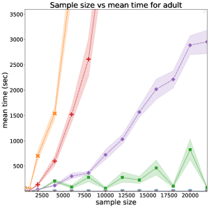
(a)

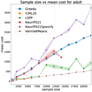
(b)

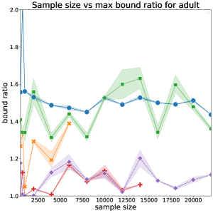
(c)

Figure 1: Mean completion time, cost, and bound ratio for the algorithms on Gowalla dataset subsampled to different sizes, $k=10$. The shades represent the $95\%$ confidence interval (notice that some algorithms are deterministic). Runs that did not complete in $1$ hour on the sample are not reported. VanillaKMeans bound ratio is > 60 in all runs and not show in the plot as out of scale).

Metrics. We focus on three key metrics: the $k$-means cost of clustering, the average runtime of algorithm and the bound ratio $\max_{p}\frac{\text{dist}(p,S)}{\delta(p)}$ where $S$ is the solution of the algorithm. We repeat each experiment configuration $10$ times and report the mean and standard deviation of the metrics.

Comparison with other baselines. In this section we report a comparison of our algorithm with the other baselines. For all experiments, unless otherwise specified, we replicate the setting of individual fairness Mahabadi and Vakilian, (2020) for $\delta(p)$, by setting $\delta(p)$ as the distance to the $\nicefrac{{n}}{{k}}$-th nearest point.

Notice that the ICML20 algorithm evaluates, for each iteration of local search, all possible swaps of one center with a non-center while NeurIPS21 and NeurIPS21Sparsify both depend on computing all-pairs distances in $O(dn^{2})$ time. This makes these algorithms not scalable to large datasets, unlike our algorithm. Therefore all prior experiments Mahabadi and Vakilian, (2020); Chakrabarty and Negahbani, (2021) used a subsample of $\approx\hskip-2.84526pt1000$ elements from the datasets to run their algorithm. In this section we use a similar approach for consistency.

In Figure 1(a), 1(b), 1(c), we report the results of the various algorithms for different sizes of the sample on the gowalla dataset, fixing $k=10$.

The main message of the paper is summarized in Figure 1(a). We allowed each algorithm to run for up to $1$ hour on increasingly large samples of the data. Notice how our algorithm is orders of magnitude faster than all fair baselines including the faster NeurIPS21Sparsify variant. ICML20 does not complete in $1$ hour past size $\sim 5000$, NeurIPS21 past $\sim 7000$, NeurIPS21Sparsify past $\sim 25000$ while our algorithm’s running time is not highly affected by scale. This will allow us to run on $500,000$ sized datasets, orders of magnitude larger than SOTA algorithms.

Then we focus on the $k$-means cost of the solution in Figure 1(b). Notice that our algorithm (LSPP) has a cost better (or comparable) than that of all fair baselines and close to the unfair VanillaKMeans.

Finally, Figure 1(c) shows the max ratio of distance of a point $p$ to centers vs $\delta(p)$. We observe that VanillaKMeans has a bound ratio between $60$ and $90$ (out of the plot scale), confirming the need for fair algorithms. For the remainder of the paper we will ignore VanillaKMeans.

Now we focus on the fair algorithms. Notice that the (much slower) ICML20 has statistically comparable bounds with LSPP (and both significantly better than their worst case guarantees), while NeurIPS21 and NeurIPS21Sparsify have slightly better bounds.

Experiments on the full datasets.

The scalability of our algorithm allows us to run it on the full datasets with up to $\nicefrac{{1}}{{2}}$ million elements. In this section, we run our algorithm and the fast Greedy baseline on all complete datasets, using $k=10$. Our algorithm completed all runs in less than $2$ hours on the full datasets.

To compare with all the slower baselines we allow ICML20, NeurIPS21 and NeurIPS21Sparsify to run on a subsample of the data containing 4000 points (but we evaluate the solution on the entire dataset). This of course has no theoretical guarantee and can perform especially poorly in case of outliers. In the supplementary material we report the standard deviation for the metrics in Table 1.

For this large-scale experiment, the input bound $\delta(p)$ for each point $p$ is set using the $\nicefrac{{n}}{{k}}$-th closest point in a random sample of 1000 elements.

In all but one dataset, our algorithm has a significantly lower $k$-means cost than that of all other baselines. Similarly to the above results, our algorithm has a similar or better ratio bound than that of ICML20 (with the sampling heuristic), while the ratio bound of NeurIPS21 and NeurIPS21Sparsify is sometimes lower. In any instance our algorithm has a much better ratio that the worst-case theoretical guarantees. The results are reported in Table 1.

dataset	algorithm	$k$-means cost	bound ratio
adult	Greedy	1.56E+05	1.8
	ICML20	6.59E+04	1.4
	NeurIPS21	1.14E+05	1.2
	NeurIPS21Sparsify	1.02E+05	1.2
	LSPP	6.14E+04	1.4
bank	Greedy	8.57E+04	1.9
	ICML20	3.23E+04	1.6
	NeurIPS21	5.68E+04	1.2
	NeurIPS21Sparsify	5.70E+04	1.2
	LSPP	3.02E+04	1.6
covtype	Greedy	3.33E+07	1.3
	ICML20	2.84E+07	1.1
	NeurIPS21	2.76E+07	1.1
	NeurIPS21Sparsify	2.80E+07	1.1
	LSPP	2.50E+07	1.1
diabetes	Greedy	6.60E+04	2.7
	ICML20	3.00E+04	1.3
	NeurIPS21	N/A	N/A
	NeurIPS21Sparsify	3.36E+04	1.2
	LSPP	2.66E+04	1.4
gowalla	Greedy	1.17E+04	1.6
	ICML20	N/A	N/A
	NeurIPS21	8.65E+03	1.1
	NeurIPS21Sparsify	1.63E+04	1.2
	LSPP	6.93E+03	1.6
shuttle	Greedy	4.89E+05	2.3
	ICML20	1.91E+05	2.0
	NeurIPS21	2.60E+05	1.0
	NeurIPS21Sparsify	2.72E+05	1.1
	LSPP	1.79E+05	2.1
skin	Greedy	1.80E+05	2.1
	ICML20	7.47E+04	1.8
	NeurIPS21	9.36E+04	1.1
	NeurIPS21Sparsify	1.03E+05	1.1
	LSPP	9.27E+04	3.1

Table 1: Mean Cost and max bound ratio for all full-sized datasets and k=10 with ICML20, NeurIPS21 and NeurIPS21Sparsify ran on a sample of 4000 points.

Finally, we focus on the impact of our novel F-Lloyd’s fair improvement method. We observe that this step can only be applied to algorithms based on anchor points (like ours and ICML20) and that (of course) cannot improve the efficiency of the slow ICML20 baseline. For this reason we tested ICML20 with our F-Lloyd method on a sample of size $1000$ points where such an algorithm can run. The full analysis is reported in the supplemental material and confirms all prior experiments. We observe that adding F-Lloyd steps improves the cost of ICML20 baseline as well, but does not change the overall trend reported, i.e., that our algorithm has comparable (or better cost) than all fair baselines while scaling to orders of magnitude larger datasets. We believe that the F-Lloyd algorithm could benefit other work in the future.

5 Conclusions and Future Works

We present a new scalable algorithm for individually fair clusters, with strong theoretical guarantees and good experimental performances. An interesting open question is to use the more recent analysis of LocalSearch++ by Choo et al., (2020) to improve the running time of our algorithm to $O(dnk^{2})$. However, it is not clear how to obtain the necessary strong guarantees similar to the one in Lemma 12 of Choo et al., (2020).

6 Additional experimental results

Small scale datasets and effect of F-Lloyd improvement

The results observed before are confirmed in all datasets, as shown in Table 2, where we report the cost and bound ratio for all datasets, subsampled to 1000 elements, and $k=10$.

In this experiment we report as well the results of using our novel F-Lloyd’s fair improvement method on top of the ICML20 baseline (recall that this step can only be applied to algorithms based on anchor points such as LSPP and ICML20). Even with this improvement, the picture remains unchanged LSPP has always the lowest cost (or close to lowest cost, achieved by the improved ICML20+F-Lloyd) to all fair algorithms while scaling to $2$ orders of magnitude larger datasets than ICML20 (even without the additional running time of F-Lloyd which only makes ICML20 slower). For this reason, for the remainder of the paper we focus on the ICML20 baseline as introduced by the authors.

Effect of $k$

A similar overall picture appears in Figure 2(a), 2(b), where we report the results of the various algorithms for different $k$’s on a sample of 1000 elements in the adult dataset. Notice that our algorithm has lower or comparable cost to all fair baselines in cost in Figure 2(a) and the comparable or slightly higher bound ratio in Figure 2(b).

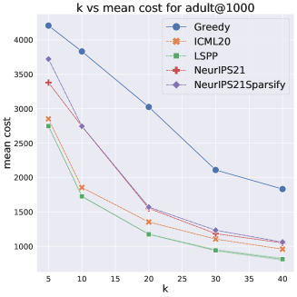
(a)

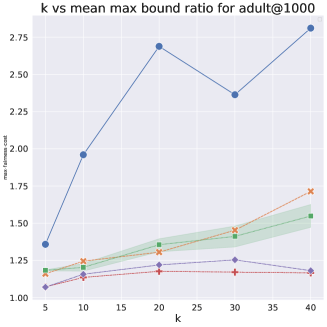
(b)

Figure 2: Mean completion cost and bound ratio for the algorithms on the adult dataset subsampled to 1000 elements and different $k$’s. The shades represent the $95\%$ confidence interval.

Additional results on large-scale datasets

As we mentioned before, our algorithm is the only one that runs on the big datasets within reasonable time (and memory).

To compare with all the slower baselines we allow ICML20, NeurIPS21 and NeurIPS21Sparsify to run on a subsample of the data containing 4000 points (but we evaluate the solution on the entire dataset). This of course has no theoretical guarantee and can perform especially poorly in case of outliers.

For this large-scale experiment, the input bound $\delta(p)$ for each point $p$ is set using the $\nicefrac{{n}}{{k}}$-th closest point in a random sample of 1000 elements.

The results in Table 1 shows that in all but one dataset, our algorithm has a significantly lower $k$-means cost than that of all other baselines. Similarly to the above results, our algorithm has a similar or better ratio bound than that of ICML20 (with the sampling heuristic), while the ratio bound of NeurIPS21 and NeurIPS21Sparsify is sometimes lower. In any instance our algorithm has a much better ratio that the worst-case theoretical guarantees.

dataset	algorithm	$k$-means cost	bound ratio
adult	Greedy	3832.6 (—)	2.0 (—)
	ICML20	1854.9 (—)	1.2 (—)
	ICML20+F-Lloyd	1733.2 (—)	1.3 (—)
	NeurIPS21	2744.3(—)	1.1 (—)
	NeurIPS21Sparsify	2745.5 (—)	1.2 (—)
	LSPP	1726.0 (9.4)	1.2 (0)
bank	Greedy	1081.8 (—)	1.8 (—)
	ICML20	568.4 (—)	1.4 (—)
	ICML20+F-Loyd	517.9 (—)	1.5 (—)
	NeurIPS21	784.2 (—)	1.2 (—)
	NeurIPS21Sparsify	761.2 (—)	1.2 (—)
	LSPP	510.5 (6.9)	1.4 (0.1)
covtype	Greedy	50629.8 (—)	1.3 (—)
	ICML20	42121.5 (—)	1.1 (—)
	ICML20+F-Lloyd	35211.3 (—)	1.0 (—)
	NeurIPS21	47810.6 (—)	1.1(—)
	NeurIPS21Sparsify	46078.6 (—)	1.1 (—)
	LSPP	35860.4 (569)	1.0 (0.0)
diabetes	Greedy	522.3 (—)	2.1 (—)
	ICML20	266.4 (—)	1.1 (—)
	ICML200+F-Loyd	231.8 (—)	1.1 (—)
	NeurIPS21	N/A	N/A
	NeurIPS21Sparsify	299.8 (—)	1.1 (—)
	LSPP	248.5 (8.5)	1.2 (0.2)
gowalla	Greedy	41.4 (—)	1.6 (—)
	ICML20	18.6 (—)	1.0 (—)
	ICML200+F-Lloyd	17.3 (—)	1.0 (—)
	NeurIPS21	44.3 (—)	1.0 (—)
	NeurIPS21Sparsify	68.6 (—)	1.0 (—)
	LSPP	20.3 (1.6)	1.3 (0.1)
shuttle	Greedy	2647.4 (—)	2.0 (—)
	ICML20	1335.0 (—)	1.8 (—)
	ICML200+F-Lloyd	1272.1 (—)	1.8 (—)
	NeurIPS21	2494.8 (—)	1.0(—)
	NeurIPS21Sparsify	2477.1 (—)	1.2 (—)
	LSPP	1219.1 (31.3)	1.8 (0.1)
skin	Greedy	584.3 (—)	2.7 (—)
	ICML20	292.8(—)	2.3 (—)
	ICML200+F-Lloyd	276.2 (—)	2.4 (—)
	NeurIPS21	379.4 (—)	1.1 (—)
	NeurIPS21Sparsify	384.1 (—)	1.1 (—)
	LSPP	314.3 (27.7)	2.5 (0.1)

Table 2: Cost and max bound ratio for all datasets subsampled for 1000 elements and $k=10$ (stddev in parentheses for the LSPP randomized algorithm). N/A indicates that the algorithm did not complete in 2 hours. In this table we also report experiments with the F-Lloyd heuristic applied to ICML20.

Standard deviation of the metrics in large datasets.

In Table 3 we report the standard deviation for the metrics in Table 1. Notice that in this experiment, the input to ICML20, NeurIPS21 and NeurIPS21Sparsify algorithms are run on a random subsample, so this makes the algorithm non-deterministic. Notice that our algorithm has statistically significantly lower cost than the other baselines in almost all datasets.

dataset	algorithm	cost stddev	bound ratio stddev
adult	ICML20	6.81E+02	1.00E-01
	NeurIPS21	1.34E+04	0.00E+00
	NeurIPS21Sparsify	7.65E+03	0.00E+00
	LSPP	8.84E+02	0.00E+00
bank	ICML20	1.04E+03	1.00E-01
	NeurIPS21	5.95E+03	0.00E+00
	NeurIPS21Sparsify	6.57E+03	0.00E+00
	LSPP	6.85E+02	1.00E-01
covtype	ICML20	2.23E+05	0.00E+00
	NeurIPS21	1.85E+05	0.00E+00
	NeurIPS21Sparsify	3.83E+05	0.00E+00
	LSPP	4.51E+05	0.00E+00
diabetes	ICML20	8.19E+02	2.00E-01
	NeurIPS21	N/A	N/A
	NeurIPS21Sparsify	1.22E+03	1.00E-01
	LSPP	9.58E+02	1.00E-01
gowalla	ICML20	N/A	N/A
	NeurIPS21	2.07E+03	0.00E+00
	NeurIPS21Sparsify	4.05E+03	1.00E-01
	LSPP	1.32E+03	0.00E+00
shuttle	ICML20	1.25E+04	2.00E-01
	NeurIPS21	6.57E+03	0.00E+00
	NeurIPS21Sparsify	1.37E+04	0.00E+00
	LSPP	1.05E+04	3.00E-01
skin	ICML20	3.51E+03	3.00E-01
	NeurIPS21	1.60E+03	1.00E-01
	NeurIPS21Sparsify	1.31E+04	0.00E+00
	LSPP	4.80E+02	2.00E-01

Table 3: Standard deviation of cost and max bound ratio for all full-sized datasets and k=10 with ICML20, NeurIPS21 and NeurIPS21Sparsify ran on a sample of 4000 points .

Effect of the normalization of the points.

In our experiments, we applied two preprocessing steps that are common in the clustering literature Borassi et al., (2020): each point in the dataset is shifted so that the dataset has zero mean; and each dimension is scaled to have unit standard deviation. We have observed that such pre-processing has no significant effect on the experimental conclusion of our work. In Table 4 we report results for the same experiments previously reported in Table 1, this time executed on the adult dataset without normalization.

As observed before, our algorithm has a significantly lower (or comparable) $k$-means cost than that of other baselines, better ratio than the worst-case theoretical guarantees and a much faster runtime than all fair algorithms.

		$k$-means-cost	max-fairness-cost
dataset	algorithm
adult (no norm.)	Greedy	5.0E+13	2.9E+00
	ICML20	1.2E+13	1.8E+00
	NeurIPS21	N/A	N/A
	NeurIPS21Sparsify	5.2E+13	1.8E+00
	LSPP	1.3E+13	2.3E+00

Table 4: Mean Cost and max bound ratio for all full-sized datasets and k=10 with ICML20, NeurIPS21 and NeurIPS21Sparsify ran on a sample of 4000 points on the Adult datasets without normalization.

7 Seeding Strategy for Local Search

We describe the seeding procedure outlined in algorithm 3 to initialize our local-search approach. The proof of this lemma can be found in Section 7.

Lemma 7.1.

If the problem is feasible, Algorithm 3 with parameter $\gamma>2$ returns a set of points $S$ of size at most $k$ such that each point $p$ is at distance at most $\gamma\delta(p)$ from the closest point in $S$, i.e., $\forall p\in A:\text{dist}(p,S)\leq\gamma\delta(p)$.

Proof of Lemma 7.1.

The proof is similar to the proof of correctness of Gonzales’ algorithm for $k$-center Gonzalez, (1985) and of Hochbaum and Shmoys’ algorithm Hochbaum and Shmoys, (1985). Observe first that by feasibility, there cannot be $k+1$ points $p^{\prime}_{1},\ldots,p^{\prime}_{k+1}$ such that the balls $\delta(p^{\prime}_{i})$ are all pairwise disjoint (since otherwise the optimum solution would need $k+1$ centers to satisfy the $\delta(p^{\prime})$ constraints).

Let $p_{1},\ldots,p_{k^{*}}$ be the sequence of points picked by the algorithm. We have that $\delta(p_{i})\leq\delta(p_{j})$ for any $i\leq j$. Note that at the end of the algorithm, each point $p$ is at distance at most $\gamma\delta(p)$ from one of $p_{1},\ldots,p_{k^{*}}$ so what remains to be shown is that $k^{*}\leq k$. We claim that the collection of balls centered at the $p_{i}$ and of radii $\delta(p_{i})$ are all pairwise disjoint and so if the problem is feasible, the algorithm does not return more than $k$ points (i.e.: $k^{*}\leq k$). Consider a pair $i,j$ and without loss of generality $i>j$. We have that $p_{i}$ is at distance at least $\gamma\delta(p_{i})$ from $p_{j}$ by the definition of the algorithm. Since $\gamma>2$ and $\delta(p_{i})\geq\delta(p_{j})$, we have that $\delta(p_{i})+\delta(p_{j})\leq 2\delta(p_{i})<\gamma\delta(p_{i})\leq\text{dist}(p_{i},p_{j})$ and so the ball of radius $\delta(p_{j})$ around $p_{j}$ cannot intersect the ball of radius $\delta(p_{i})$ around $p_{i}$.

∎

8 Proof of Section 3

The proof in this section follows closely the structure of the proofs in Lattanzi and Sohler, (2019) with some modification to carefully handle the anchor zones constraints.

8.1 Proof of Theorem 1.1

Proof of Theorem 1.1.

Observe that the dimension can be reduced to $O(\log k/\varepsilon^{-2})$ using the Johnson-Lindenstrauss transform Becchetti et al., (2019); Makarychev et al., (2019). Hence, in $\tilde{O}(nd)$ time one can find a projection to a space of dimension $O(\log k)$ that preserves the $k$-means cost of all solutions up to an $O(1)$ factor and execute the algorithm in this space. The claimed running time then follows immediately.

The algorithm returns infeasible only if it finds $k+1$ disjoint individual fairness balls. But in that case, the problem is infeasible (their fairness constraints cannot be satisfied with $k$ points).

Let $\hat{S}$ be the set $S$ before calling ConstrainedLocalSearch++. In this set, every point $p$ has distance at most $\gamma\delta(p)$ from a center so $\text{cost}(X,\hat{S})\leq\gamma n\Delta^{2}$. lemma 3.2 then shows that after $Z$ calls to ConstrainedLocalSearch++, we obtain a constant approximation.

Now we show that at any point in time during the execution of the algorithm $\max_{p\in X}\text{dist}(p,S)\leq 2\gamma\delta(p)$. The algorithm guarantees to keep at least one point in every anchor ball. Moreover every point $p$ is at distance at most $\gamma\delta(p)$ from an anchor point $p^{\prime}$ with $\delta(p)>\delta(p^{\prime})$. The anchor ball $B(p^{\prime})$ must have a center $c\in S$, so $\text{dist}(c,p^{\prime})\leq\gamma\delta(p^{\prime})$. Thus by triangle inequality $\text{dist}(c,p)\leq 2\gamma\delta(p)$.

It takes $O(dnk)$ time to compute the initial set $\hat{S}$. To implement the local search, we need to compute the cost of swapping the new sample point with an old center. This requires iterating over all clusters and for each cluster we need to compute the distance to all other centers and to check that there is at least one center in each anchor ball. Thus, a local search step requires $O(dkn+dk)$ time in the worst case, resulting in a total runtime of $O(dnkZ)$. The Theorem follows. ∎

8.2 Proof of Lemma 3.2

Proof.

By Lemma 3.1 we know that if before any call of ConstrainedLocalSearch++ the cost of the centers is bigger than $2000\text{Opt}_{k}$ then with probability $\frac{1}{1000}$ we reduce the cost by a $(1-\frac{1}{100k})$ multiplicative factor.

Now consider another random process $Y$ with initial value equal to $\text{cost}(X,\hat{S})$, which for $Z=100000k\log n\Delta(X)^{2}$ iterations, it reduces the value by a $\left(1-\frac{1}{100k}\right)$ multiplicative factor with probability $1/1000$, and finally increases the value by an additive $2000\text{Opt}_{k}$. It is not hard to see that the final value of $Y$ stochastically dominates the cost of the solution our algorithm produces.

So the final expected value of $Y$ is larger than the expected value of $\text{cost}(X,S)$ conditioned on the initial clustering $\hat{S}$. Furthermore,

$$E[Y] =2000\text{Opt}_{k}+\text{cost}(X,\hat{S})\cdot\sum_{i=0}^{Z}\genfrac{(}{)}{0.0pt}{0}{Z}{i}\left(\frac{1}{1000}\right)^{i}\left(\frac{999}{1000}\right)^{Z-i}\left(1-\frac{1}{100k}\right)^{i}$$

$$=\text{cost}(X,\hat{S})\left(1-\frac{1}{100000k}\right)^{Z}+2000\text{Opt}_{k}$$

$$\leq\frac{\text{cost}(X,\hat{S})}{n\Delta(X)^{2}}+2000\text{Opt}_{k}.$$

This implies that $E[\text{cost}(X,S)|\hat{S}]\leq\frac{\text{cost}(X,\hat{S})}{n\Delta(X)^{2}}+2000\text{Opt}_{k}$. Our upper-bound on the cost of $\hat{S}$ is deterministic, hence $E[\text{cost}(X,S)]\leq\frac{\text{cost}(X,\hat{S})}{n\Delta(X)^{2}}+2000\text{Opt}_{k}\leq 2001\text{Opt}_{k}$. ∎

This section contains the proofs of the lemmas of Section 3.

8.3 Proof of Lemma 3.2

The proof in this section follows closely the structure of the proofs in Lattanzi and Sohler, (2019) and we include it for completeness.

Proof of Lemma 3.2.

By Lemma 3.1 we know that if before any call of ConstrainedLocalSearch++ the cost of the centers is bigger than $2000\text{Opt}_{k}$ then with probability $\frac{1}{1000}$ we reduce the cost by a $(1-\frac{1}{100k})$ multiplicative factor.

We next use another random process $Y$ to handle dependencies between rounds. In this way we can have a coupling with an independent process that is easier to analyze. We let $Y$ be a random process with initial value equal to $\text{cost}(X,\hat{S})$, which for $Z=100000k\log n\Delta^{2}$ iterations, it reduces the value by a $\left(1-\frac{1}{100k}\right)$ multiplicative factor with probability $1/1000$, and finally increases the value by an additive $2000\text{Opt}_{k}$. It is not hard to see that the final value of $Y$ stochastically dominates the cost of the solution our algorithm produces. So the final expected value of $Y$ is larger than the expected value of $\text{cost}(X,S)$ conditioned on the initial clustering $\hat{S}$. Furthermore,

$$E[Y] =2000\text{Opt}_{k}+\text{cost}(X,\hat{S})\cdot\sum_{i=0}^{Z}\genfrac{(}{)}{0.0pt}{0}{Z}{i}\left(\frac{1}{1000}\right)^{i}\left(\frac{999}{1000}\right)^{Z-i}\left(1-\frac{1}{100k}\right)^{i}$$

$$=\text{cost}(X,\hat{S})\left(1-\frac{1}{100000k}\right)^{Z}+2000\text{Opt}_{k}$$

$$\leq\frac{\text{cost}(X,\hat{S})}{n\Delta^{2}}+2000\text{Opt}_{k}.$$

This implies that $E[\text{cost}(X,S)|\hat{S}]\leq\frac{\text{cost}(X,\hat{S})}{n\Delta^{2}}+2000\text{Opt}_{k}$. Our upper-bound on the cost of $\hat{S}$ is deterministic, hence $E[\text{cost}(X,S)]\leq\frac{\text{cost}(X,\hat{S})}{n\Delta^{2}}+2000\text{Opt}_{k}\leq 2001\text{Opt}_{k}$. ∎

8.4 Proof of Proposition 3.5

Proof of Proposition 3.5.

If $c^{\prime}$ is within distance $\gamma\delta(a)$ to $a$, the lemma follows from $\text{dist}(c^{*},c)=\text{dist}(c^{*},c^{\prime})$ by definition of $c$ and anchor ball. Otherwise we know that $c^{*}$ is at distance at most $\delta$ from $a$, $c$ is at distance at most $\gamma\delta$ from $a$, and $c^{\prime}$ is at distance at least $\gamma\delta$ from $a$. The lemma follows the triangle inequality. ∎

8.5 Proof of Lemma 3.7

Proof of Lemma 3.7.

We only present the case $r\in H$. The case $r\in L$ is almost identical (in fact, simpler). We observe that $\text{reassign}(X,S,c_{r})=\text{cost}(X_{r}\setminus X_{r}^{*},S\setminus\{r\})-\text{cost}(X_{r}\setminus X_{r}^{*},S)$ since vertices in clusters other than $X_{r}$ will still be assigned to their current center. If $r\in H$, we assign every point in $X_{r}\cap X_{i}^{*}$, $i\not=r$, to the center that captured the center of $X_{i}^{*}$. While this assignment may not be optimal, its cost provides an upper bound on the cost of reassigning the points: We move every point in $X_{r}\cap X_{i}^{*}$, $i\not=r$, to the center of $X_{i}^{*}$. Now the closest center of $S$ to these points is a center with distance close to the one that captured the center of $X_{i}^{*}$, which, for points not in $X_{r}^{*}$, cannot be $r$, since $r$ is in $H$. The fact that the squared moved distance of each point equals its contribution to the optimal solution allows us to get an upper bound on the cost change using lemma 3.4. After this, we move the points back to their original location while keeping their cluster assignments fixed. Again we can use the bound on the overall moved distance together with lemma 3.4 to obtain a bound on the change of cost. Combining the two gives an upper bound on the increase of cost that comes from reassigning the points. Details follow.

Let $Q_{r}$ be the (multi)set of points obtained from $X_{r}\setminus X_{r}^{*}$ by moving each point in $X_{i}^{*}\cap X_{r}$, $i\not=r$, to $c_{i}^{*}$. We apply lemma 3.4 with $\epsilon=1/100$ to get an upper bound for the change of cost with respect to $S$ that results from moving the points to $Q_{r}$. For $p\in X_{r}\setminus X_{r}^{*}$ let $q_{p}\in Q_{r}$ be the point of $Q_{r}$ to which $p$ has been moved. We have:

$$|\text{cost}(\{p\},S)-\text{cost}(\{q_{p}\},S)|\leq\frac{1}{100}\text{cost}(\{p\},S)+101\cdot\text{cost}(\{p\},S^{*}).$$

Summing up over all points in $X_{r}\setminus X_{r}^{*}$ yields

$$|\text{cost}(X_{r}\setminus X_{r}^{*},S)-\text{cost}(Q_{r},S)|\leq\frac{1}{100}\text{cost}(X_{r}\setminus X_{r}^{*},S)+101\cdot\text{cost}(X_{r}\setminus X_{r}^{*},S^{*}).$$

Let $Q_{r,i}$ be the points in $Q_{r}$ that are nearest to center $c_{i}\in S$ and let $X_{r,i}$ be the set of their original locations. For $p\in X_{r,i}$ that has been moved to $q_{p}\in Q_{r,i}$ with $q_{p}$ let $c_{i}^{\prime}$ be the closest point to $q_{p}$ not equal to $r$. Note that the only case in which $c_{i}\neq c_{i}^{\prime}$ is when $c_{i}=r$. Furthermore, $q_{p}$ is not captured by $r$ because $r$ captures $c_{r}^{*}$ and is in $H$. So by proposition 3.5 we know $\text{cost}(\{q_{p}\},\{c_{i}^{\prime}\})\leq\frac{\mu+1}{\mu-1}\text{cost}(\{q_{p}\},\{c_{i}\})$. Thus we have:

$$|\text{cost}(\{q_{p}\},\{c_{i}\})-\text{cost}(\{p\},\{c_{i}^{\prime}\})|$$

$$= |\text{cost}(\{q_{p}\},\{c_{i}\})-\text{cost}(\{q_{p}\},\{c_{i}^{\prime}\})|+|\text{cost}(\{q_{p}\},\{c_{i}^{\prime}\})-\text{cost}(\{p\},\{c_{i}^{\prime}\})|$$

$$\leq \frac{2}{\mu-1}\text{cost}(\{q_{p}\},\{c_{i}\})+\frac{1}{100}\text{cost}(\{q_{p}\},\{c_{i}^{\prime}\})+101\cdot\text{cost}(\{p\},\{q_{p}\})$$

$$\leq \frac{1}{\mu-1}\left(2+\frac{\mu+1}{100}\right)\text{cost}(\{q_{p}\},\{c_{i}\})+101\cdot\text{cost}(\{p\},\{q_{p}\}),$$

where in the first inequality we used lemma 3.4 with $\epsilon=1/100$.

Summing up over all points in $X_{r}\setminus X_{r}^{*}$ and the corresponding points in $Q_{r}$ yields

$$|\text{cost}(Q_{r},S)-\sum_{i}\text{cost}(X_{r,i},S\setminus\{r\})|$$

$$\leq \frac{1}{\mu-1}\left(2+\frac{\mu+1}{100}\right)\text{cost}(Q_{r},S)+101\cdot\text{cost}(X_{r}\setminus X_{r}^{*},S^{*})$$

$$\leq \frac{26}{25}\bigg{(}\frac{11}{100}\text{cost}(X_{r}\setminus X_{r}^{*},S)+\hskip 17.07164pt101\cdot\text{cost}(X_{r}\setminus X_{r}^{*},S^{*})\bigg{)}+$$

$$101\cdot\text{cost}(X_{r}\setminus X_{r}^{*},S^{*})$$

$$\leq \frac{3}{25}\text{cost}(X_{r},S)+231\cdot\text{cost}(X_{r},S^{*}),$$

where the second inequality uses the bound on $\mu\geq 3$. Hence,

$$\text{reassign}(X,S,c_{r})$$

$$\hskip 11.38109pt=|\text{cost}(X_{r}\setminus X_{r}^{*},S)-\sum_{i}\text{cost}(X_{r,i},S\setminus\{r\}|$$

$$\hskip 11.38109pt\leq|\text{cost}(X_{r}\setminus X_{r}^{*},S)-\text{cost}(Q_{r},S)|+|\text{cost}(Q_{r},S)-\sum_{i}\text{cost}(X_{r,i},S\setminus\{r\})|$$

$$\hskip 11.38109pt\leq\frac{13}{100}\text{cost}(X_{r},S)+332\text{cost}(X_{r},S^{*}).\qed$$

8.6 Proof of Lemma 3.9

Proof of Lemma 3.9.

We have $\sum_{h\in H}\text{cost}(X_{h}^{*},C)\geq\frac{1}{3}\text{cost}(X,S)$ and by the definition of good and lemma 3.7

$$\sum_{h\in H,h\text{ is not good}}\text{cost}(X_{h}^{*},S) \leq \sum_{h\in H}\text{reassign}(X,S,c_{h})+9\text{Opt}_{k}+\frac{1}{100}\text{cost}(X,S)$$

$$\leq \frac{14}{100}\text{cost}(X,S)+341\text{Opt}_{k}.$$

Using that $\text{cost}(X,S)\geq 2000\text{Opt}_{k}$ we obtain that

$$\sum_{h\in H,h\text{ is not good}}\text{cost}(X_{h}^{*},S)\leq\frac{621}{2000}\cdot\text{cost}(X,S).$$

So $\sum_{h\in H,h\text{ is good}}\text{cost}(X_{h}^{*},S)\geq\frac{9}{400}\cdot\text{cost}(X,S)$. The lemma follows. ∎

8.7 Proof of Lemma 3.12

Proof of Lemma 3.12.

We have $\sum_{r\in R}\text{cost}(X_{r}^{*},S)\geq 2/3\text{cost}(X,S).$ Note that $|R|\leq 2|L|$. By the definition of good and lemma 3.7

$$\sum_{r\in R,r\text{ is not good}} \text{cost}(X_{r}^{*},S)$$

$$\leq 2|L|\min_{\ell\in L}\text{reassign}(X,S,\ell)+9\text{Opt}_{k}+\frac{1}{100}\text{cost}(X,S)$$

$$\leq 2\sum_{\ell\in L}\text{reassign}(X,S,\ell)+9\text{Opt}_{k}+\frac{1}{100}\text{cost}(X,S)$$

$$\leq\frac{27}{100}\text{cost}(X,S)+673\text{Opt}_{k}.$$

Using that $\sum_{i\in\{1,\dots,k\}}\text{cost}(X_{i}^{*},S)\geq 2000\text{Opt}_{k}$ we obtain that

$$\sum_{r\in R,r\text{ is not good}}\text{cost}(X_{r}^{*},S) \leq \frac{1213}{2000}\text{cost}(X,S)$$

Now the bound follows by combining the previous inequality with

$$\sum_{r\in R}\text{cost}(X_{r}^{*},S)\geq 2/3\text{cost}(X,S)$$

. ∎

9 Further Theoretical Considerations

Our algorithms can be used to obtain an $O(1)$-approximation for the case where $C\not\subseteq X$, using the following argument. Given an instance $A,C$ where $C\not\subseteq X$, consider running our algorithm on the instance $A,C^{\prime}$ where $C^{\prime}:=A$ – hence looking at the metric induced by the points in $A$ and falling back to the setting considered in our paper. This will give a solution whose centers are in $A$. We show that we can then transform this solution into a solution whose centers are in $C$ without losing much in the approximation guarantee. To do this, we need to show the following two statements: (1) the cost of the optimum solution in the instance $A,C^{\prime}$ is at most $O(1)$ times the cost of the optimum solution in the instance $A,C$; and (2) the cost of turning the solution for $A,C^{\prime}$ into a solution for $A,C$ only loses a constant factor in the approximation guarantee.

(1) Take the optimum solution OPT for the instance $A,C$ and turn it into a solution for the instance $A,C^{\prime}$ of cost at most $O(1)$ times higher. Replace each center in Opt with the closest element in $A$. This yields a solution for $A,C^{\prime}$ (since $C^{\prime}=A$). Note that by the triangle inequality, replacing each element in Opt with the closest point in $A$ only increases the cost by a factor 4. Thus, the cost of the optimum solution for $A,C^{\prime}$ is only 4 times higher than the cost of Opt. Hence, running our algorithm on the instance $A,C^{\prime}$ yields a solution of cost $O(\text{Opt})$. We next show how to convert the solution obtained for $A,C^{\prime}$ to a solution for $A,C$.

(2) Let’s now show that we can transform any $\alpha$-approximate solution for the instance $A,C^{\prime}$ to a solution for $A,C$ without losing more than a constant factor. Indeed, for each cluster $S$ of the solution for $A,C^{\prime}$, pick the center $u_{S}$ in $C$ that is the closest to $S$ current center $c^{\prime}$ in $A^{\prime}$. For each cluster $S$, the cost obtained is by triangle inequality is at most $\sum_{s\in S}\text{dist}(s,u_{S})\leq\sum_{s\in S}\text{dist}(s,c^{\prime})+\text{dist}(c^{\prime},u_{S})\leq\sum_{s\in S}\text{dist}(s,c^{\prime})+|S|\text{dist}(c^{\prime},u_{S})$. Moreover, by the choice of $u_{S}$ and the triangle inequality, we have that $\text{dist}(c^{\prime},u_{S})\leq(1/|S|)\sum_{s\in S}(\text{dist}(s,c^{\prime})+\text{OPT}_{s}))$, where $\text{OPT}_{s}$ is the cost of $s$ in the optimum solution for $A,C$. Thus the overall cost is bounded by $\sum_{s\in S}(2\text{dist}(s,c^{\prime})+\text{OPT}_{s})$. Summing over all clusters, we have that the total cost is at most $(18\alpha+1)$ times higher than the optimum cost for the instance $A,C$. Since we prove that our algorithm is an O(1)-approx, the resulting solution is an O(1)-approx too.

References

- Abbasi et al., (2021) Abbasi, M., Bhaskara, A., and Venkatasubramanian, S. (2021). Fair clustering via equitable group representations. In Elish, M. C., Isaac, W., and Zemel, R. S., editors, FAccT, pages 504–514. ACM.
- (2) Ahmadian, S., Epasto, A., Knittel, M., Kumar, R., Mahdian, M., Moseley, B., Pham, P., Vassilvitskii, S., and Wang, Y. (2020a). Fair hierarchical clustering. In Larochelle, H., Ranzato, M., Hadsell, R., Balcan, M., and Lin, H., editors, NeurIPS.
- Ahmadian et al., (2019) Ahmadian, S., Epasto, A., Kumar, R., and Mahdian, M. (2019). Clustering without over-representation. In Proceedings of the 25th ACM SIGKDD International Conference on Knowledge Discovery & Data Mining, pages 267–275.
- (4) Ahmadian, S., Epasto, A., Kumar, R., and Mahdian, M. (2020b). Fair correlation clustering. In Chiappa, S. and Calandra, R., editors, AISTATS, volume 108 of Proceedings of Machine Learning Research, pages 4195–4205. PMLR.
- Alamdari and Shmoys, (2017) Alamdari, S. and Shmoys, D. B. (2017). A bicriteria approximation algorithm for the k-center and k-median problems. In WAOA.
- Bajpai et al., (2021) Bajpai, T., Chakrabarty, D., Chekuri, C., and Negahbani, M. (2021). Revisiting priority -center: Fairness and outliers. arXiv preprint arXiv:2103.03337.
- Becchetti et al., (2019) Becchetti, L., Bury, M., Cohen-Addad, V., Grandoni, F., and Schwiegelshohn, C. (2019). Oblivious dimension reduction for k-means: beyond subspaces and the johnson-lindenstrauss lemma. In Proceedings of the 51st Annual ACM SIGACT Symposium on Theory of Computing, STOC 2019, Phoenix, AZ, USA, June 23-26, 2019, pages 1039–1050.
- Bera et al., (2019) Bera, S. K., Chakrabarty, D., Flores, N., and Negahbani, M. (2019). Fair algorithms for clustering. In Wallach, H. M., Larochelle, H., Beygelzimer, A., d’Alché-Buc, F., Fox, E. B., and Garnett, R., editors, Advances in Neural Information Processing Systems 32: Annual Conference on Neural Information Processing Systems 2019, NeurIPS 2019, December 8-14, 2019, Vancouver, BC, Canada, pages 4955–4966.
- Beretta et al., (2023) Beretta, L., Cohen-Addad, V., Lattanzi, S., and Parotsidis, N. (2023). Multi-swap k-means++. In Advances in Neural Information Processing Systems (Neurips) 2023.
- Bhatt and Dhall, (2010) Bhatt, R. and Dhall, A. (2010). Skin segmentation dataset. UCI Machine Learning Repository.
- Blackard and Dean, (1999) Blackard, J. A. and Dean, D. J. (1999). Comparative accuracies of artificial neural networks and discriminant analysis in predicting forest cover types from cartographic variables. Computers and electronics in agriculture, 24(3):131–151.
- Borassi et al., (2020) Borassi, M., Epasto, A., Lattanzi, S., Vassilvitskii, S., and Zadimoghaddam, M. (2020). Sliding window algorithms for k-clustering problems. Advances in Neural Information Processing Systems, 33:8716–8727.
- Braverman et al., (2022) Braverman, V., Cohen-Addad, V., Jiang, S. H., Krauthgamer, R., Schwiegelshohn, C., Toftrup, M. B., and Wu, X. (2022). The power of uniform sampling for coresets. In 63rd IEEE Annual Symposium on Foundations of Computer Science, FOCS 2022, Denver, CO, USA, October 31 - November 3, 2022, pages 462–473. IEEE.
- Byrka et al., (2018) Byrka, J., Sornat, K., and Spoerhase, J. (2018). Constant-factor approximation for ordered k-median. In Diakonikolas, I., Kempe, D., and Henzinger, M., editors, STOC, pages 620–631. ACM.
- Bóta et al., (2015) Bóta, A., Krész, M., and Zaválnij, B. (2015). Adaptations of the k-means algorithm to community detection in parallel environments. In 2015 17th International Symposium on Symbolic and Numeric Algorithms for Scientific Computing (SYNASC), pages 299–302.
- Chakrabarty and Negahbani, (2021) Chakrabarty, D. and Negahbani, M. (2021). Better algorithms for individually fair -clustering. In NeurIPS.
- Chakrabarty and Swamy, (2018) Chakrabarty, D. and Swamy, C. (2018). Interpolating between k-median and k-center: Approximation algorithms for ordered k-median. In Chatzigiannakis, I., Kaklamanis, C., Marx, D., and Sannella, D., editors, ICALP, volume 107 of LIPIcs, pages 29:1–29:14. Schloss Dagstuhl - Leibniz-Zentrum für Informatik.
- Chakrabarty and Swamy, (2019) Chakrabarty, D. and Swamy, C. (2019). Approximation algorithms for minimum norm and ordered optimization problems. In Charikar, M. and Cohen, E., editors, Proceedings of the 51st Annual ACM SIGACT Symposium on Theory of Computing, STOC 2019, Phoenix, AZ, USA, June 23-26, 2019, pages 126–137. ACM.
- Chawla and Gionis, (2013) Chawla, S. and Gionis, A. (2013). k-means-: A unified approach to clustering and outlier detection. In Proceedings of the 13th SIAM International Conference on Data Mining, May 2-4, 2013. Austin, Texas, USA, pages 189–197. SIAM.
- Chhaya et al., (2022) Chhaya, R., Dasgupta, A., Choudhari, J., and Shit, S. (2022). On coresets for fair regression and individually fair clustering. In AISTATS, pages 9603–9625.
- Chierichetti et al., (2017) Chierichetti, F., Kumar, R., Lattanzi, S., and Vassilvitskii, S. (2017). Fair clustering through fairlets. In Guyon, I., von Luxburg, U., Bengio, S., Wallach, H. M., Fergus, R., Vishwanathan, S. V. N., and Garnett, R., editors, Advances in Neural Information Processing Systems 30: Annual Conference on Neural Information Processing Systems 2017, December 4-9, 2017, Long Beach, CA, USA, pages 5029–5037.
- Chlamtác et al., (2022) Chlamtác, E., Makarychev, Y., and Vakilian, A. (2022). Approximating fair clustering with cascaded norm objectives. In SODA.
- Cho et al., (2011) Cho, E., Myers, S. A., and Leskovec, J. (2011). Friendship and mobility: user movement in location-based social networks. In Proceedings of the 17th ACM SIGKDD international conference on Knowledge discovery and data mining, pages 1082–1090.
- Choo et al., (2020) Choo, D., Grunau, C., Portmann, J., and Rozhon, V. (2020). k-means++: few more steps yield constant approximation. In International Conference on Machine Learning, pages 1909–1917. PMLR.
- (25) Cohen-Addad, V., Esfandiari, H., Mirrokni, V. S., and Narayanan, S. (2022a). Improved approximations for euclidean k-means and k-median, via nested quasi-independent sets. In Leonardi, S. and Gupta, A., editors, STOC ’22: 54th Annual ACM SIGACT Symposium on Theory of Computing, Rome, Italy, June 20 - 24, 2022, pages 1621–1628. ACM.
- Cohen-Addad and Karthik C. S., (2019) Cohen-Addad, V. and Karthik C. S. (2019). Inapproximability of clustering in lp metrics. In Zuckerman, D., editor, 60th IEEE Annual Symposium on Foundations of Computer Science, FOCS 2019, Baltimore, Maryland, USA, November 9-12, 2019, pages 519–539. IEEE Computer Society.
- Cohen-Addad et al., (2021) Cohen-Addad, V., Karthik C. S., and Lee, E. (2021). On approximability of clustering problems without candidate centers. In Marx, D., editor, Proceedings of the 2021 ACM-SIAM Symposium on Discrete Algorithms, SODA 2021, Virtual Conference, January 10 - 13, 2021, pages 2635–2648. SIAM.
- (28) Cohen-Addad, V., Karthik C. S., and Lee, E. (2022b). Johnson coverage hypothesis: Inapproximability of k-means and k-median in lp-metrics. In Naor, J. S. and Buchbinder, N., editors, Proceedings of the 2022 ACM-SIAM Symposium on Discrete Algorithms, SODA 2022, Virtual Conference / Alexandria, VA, USA, January 9 - 12, 2022, pages 1493–1530. SIAM.
- Deshpande et al., (2020) Deshpande, A., Kacham, P., and Pratap, R. (2020). Robust k-means++. In Adams, R. P. and Gogate, V., editors, Proceedings of the Thirty-Sixth Conference on Uncertainty in Artificial Intelligence, UAI 2020, virtual online, August 3-6, 2020, volume 124 of Proceedings of Machine Learning Research, pages 799–808. AUAI Press.
- Dheeru and Karra Taniskidou, (2017) Dheeru, D. and Karra Taniskidou, E. (2017). UCI machine learning repository.
- Dhillon et al., (2004) Dhillon, I. S., Guan, Y., and Kulis, B. (2004). Kernel k-means: spectral clustering and normalized cuts. In Kim, W., Kohavi, R., Gehrke, J., and DuMouchel, W., editors, Proceedings of the Tenth ACM SIGKDD International Conference on Knowledge Discovery and Data Mining, Seattle, Washington, USA, August 22-25, 2004, pages 551–556. ACM.
- Dorabiala et al., (2021) Dorabiala, O., Kutz, J. N., and Aravkin, A. Y. (2021). Robust trimmed k-means. CoRR, abs/2108.07186.
- Feldman et al., (2018) Feldman, D., Schmidt, M., and Sohler, C. (2018). Turning big data into tiny data: Constant-size coresets for k-means, PCA and projective clustering. CoRR, abs/1807.04518.
- Froese et al., (2022) Froese, V., Kellerhals, L., and Niedermeier, R. (2022). Modification-fair cluster editing. In Proceedings of the AAAI Conference on Artificial Intelligence, volume 36, pages 6631–6638.
- Georgogiannis, (2016) Georgogiannis, A. (2016). Robust k-means: a theoretical revisit. In Lee, D. D., Sugiyama, M., von Luxburg, U., Guyon, I., and Garnett, R., editors, Advances in Neural Information Processing Systems 29: Annual Conference on Neural Information Processing Systems 2016, December 5-10, 2016, Barcelona, Spain, pages 2883–2891.
- Ghadiri et al., (2021) Ghadiri, M., Samadi, S., and Vempala, S. S. (2021). Socially fair k-means clustering. In Elish, M. C., Isaac, W., and Zemel, R. S., editors, FAccT, pages 438–448. ACM.
- Gonzalez, (1985) Gonzalez, T. F. (1985). Clustering to minimize the maximum intercluster distance. Theoretical computer science, 38:293–306.
- Gupta et al., (2023) Gupta, S., Ghalme, G., Krishnan, N. C., and Jain, S. (2023). Efficient algorithms for fair clustering with a new notion of fairness. Data Mining and Knowledge Discovery, pages 1–39.
- Hochbaum and Shmoys, (1985) Hochbaum, D. S. and Shmoys, D. B. (1985). A best possible heuristic for the k-center problem. Math. Oper. Res., 10(2):180–184.
- Hotegni et al., (2023) Hotegni, S. S., Mahabadi, S., and Vakilian, A. (2023). Approximation algorithms for fair range clustering. In International Conference on Machine Learning, pages 13270–13284. PMLR.
- Humayun et al., (2021) Humayun, A. I., Balestriero, R., Kyrillidis, A., and Baraniuk, R. (2021). No more than 6ft apart: robust -means via radius upper bounds. under submission.
- Jung et al., (2020) Jung, C., Kannan, S., and Lutz, N. (2020). Service in your neighborhood: Fairness in center location. In Roth, A., editor, FORC, volume 156 of LIPIcs, pages 5:1–5:15. Schloss Dagstuhl - Leibniz-Zentrum für Informatik.
- Kalhan et al., (2019) Kalhan, S., Makarychev, K., and Zhou, T. (2019). Correlation clustering with local objectives. In Wallach, H., Larochelle, H., Beygelzimer, A., d'Alché-Buc, F., Fox, E., and Garnett, R., editors, Advances in Neural Information Processing Systems, volume 32. Curran Associates, Inc.
- Kanungo et al., (2002) Kanungo, T., Mount, D. M., Netanyahu, N. S., Piatko, C. D., Silverman, R., and Wu, A. Y. (2002). A local search approximation algorithm for k-means clustering. In Hurtado, F., Sacristán, V., Bajaj, C., and Suri, S., editors, Proceedings of the 18th Annual Symposium on Computational Geometry, Barcelona, Spain, June 5-7, 2002, pages 10–18. ACM.
- Kleindessner et al., (2019) Kleindessner, M., Awasthi, P., and Morgenstern, J. (2019). Fair k-center clustering for data summarization. In Chaudhuri, K. and Salakhutdinov, R., editors, Proceedings of the 36th International Conference on Machine Learning, ICML 2019, 9-15 June 2019, Long Beach, California, USA, volume 97 of Proceedings of Machine Learning Research, pages 3448–3457. PMLR.
- Kohavi et al., (1996) Kohavi, R. et al. (1996). Scaling up the accuracy of naive-bayes classifiers: A decision-tree hybrid. In Kdd, volume 96, pages 202–207.
- Lattanzi and Sohler, (2019) Lattanzi, S. and Sohler, C. (2019). A better k-means++ algorithm via local search. In International Conference on Machine Learning, pages 3662–3671. PMLR.
- Lloyd, (1982) Lloyd, S. P. (1982). Least squares quantization in PCM. IEEE Trans. Inf. Theory, 28(2):129–136.
- MacQueen, (1967) MacQueen, J. B. (1967). Some methods for classification and analysis of multivariate observations. In Cam, L. M. L. and Neyman, J., editors, Proc. of the fifth Berkeley Symposium on Mathematical Statistics and Probability, volume 1, pages 281–297. University of California Press.
- Mahabadi and Vakilian, (2020) Mahabadi, S. and Vakilian, A. (2020). Individual fairness for k-clustering. In ICML, volume 119 of Proceedings of Machine Learning Research, pages 6586–6596. PMLR.
- Makarychev et al., (2019) Makarychev, K., Makarychev, Y., and Razenshteyn, I. P. (2019). Performance of johnson-lindenstrauss transform for k-means and k-medians clustering. In Charikar, M. and Cohen, E., editors, Proceedings of the 51st Annual ACM SIGACT Symposium on Theory of Computing, STOC 2019, Phoenix, AZ, USA, June 23-26, 2019, pages 1027–1038. ACM.
- Makarychev and Vakilian, (2021) Makarychev, Y. and Vakilian, A. (2021). Approximation algorithms for socially fair clustering. In Belkin, M. and Kpotufe, S., editors, Conference on Learning Theory, COLT 2021, 15-19 August 2021, Boulder, Colorado, USA, volume 134 of Proceedings of Machine Learning Research, pages 3246–3264. PMLR.
- Moro et al., (2014) Moro, S., Cortez, P., and Rita, P. (2014). A data-driven approach to predict the success of bank telemarketing. Decision Support Systems, 62:22–31.
- Plesník, (1987) Plesník, J. (1987). A heuristic for the p-center problems in graphs. Discret. Appl. Math., 17(3):263–268.
- Raykov et al., (2016) Raykov, Y. P., Boukouvalas, A., Baig, F., and Little, M. A. (2016). What to do when k-means clustering fails: A simple yet principled alternative algorithm. PLOS ONE, 11(9):1–28.
- Rösner and Schmidt, (2018) Rösner, C. and Schmidt, M. (2018). Privacy preserving clustering with constraints. In Chatzigiannakis, I., Kaklamanis, C., Marx, D., and Sannella, D., editors, 45th International Colloquium on Automata, Languages, and Programming, ICALP 2018, July 9-13, 2018, Prague, Czech Republic, volume 107 of LIPIcs, pages 96:1–96:14. Schloss Dagstuhl - Leibniz-Zentrum für Informatik.
- Vakilian and Yalçiner, (2022) Vakilian, A. and Yalçiner, M. (2022). Improved approximation algorithms for individually fair clustering. In AISTATS.
- Wang et al., (2020) Wang, X., Fan, S., Kuang, K., Shi, C., Liu, J., and Wang, B. (2020). Decorrelated clustering with data selection bias. In Bessiere, C., editor, Proceedings of the Twenty-Ninth International Joint Conference on Artificial Intelligence, IJCAI 2020, pages 2177–2183. ijcai.org.
- Zhang et al., (2007) Zhang, S., Wang, R.-S., and Zhang, X.-S. (2007). Identification of overlapping community structure in complex networks using fuzzy -means clustering. Physica A: Statistical Mechanics and its Applications, 374:483–490.