Hilbert-Space Ergodicity in Driven Quantum Systems:
Obstructions and Designs

Abstract

Despite its long history, a canonical formulation of quantum ergodicity that applies to general classes of quantum dynamics, including driven systems, has not been fully established. Here we introduce and study a notion of quantum ergodicity for closed systems with time-dependent Hamiltonians, defined as statistical randomness exhibited in their long-time dynamics. Concretely, we consider the temporal ensemble of quantum states (time-evolution operators) generated by the evolution, and investigate the conditions necessary for them to be statistically indistinguishable from uniformly random states (operators) in the Hilbert space (space of unitaries). We find that the number of driving frequencies underlying the Hamiltonian needs to be sufficiently large for this to occur. Conversely, we show that statistical pseudo-randomness — indistinguishability up to some large but finite moment, can already be achieved by a quantum system driven with a single frequency, i.e., a Floquet system, as long as the driving period is sufficiently long. Our work relates the complexity of a time-dependent Hamiltonian and that of the resulting quantum dynamics, and offers a fresh perspective to the established topics of quantum ergodicity and chaos from the lens of quantum information.

I Introduction

Ergodicity in classical systems is a well-established, unambiguous concept: it is the property of dynamics exploring all allowed configurations, irrespective of initial state. Quantum ergodicity, on the other hand, is formulated rather differently, and typically in an inherently non-dynamical fashion [1, 2]: in systems with a semiclassical limit, it is taken to be the feature of high-energy eigenstates having probability densities weakly tending to a uniform distribution in phase space [3]. This definition though, does not cover all quantum systems, as there are many Hamiltonians without an obvious semiclassical limit, e.g., systems of interacting qubits. Instead, an appeal is often made to statistical similarities of the distribution of energy levels and associated energy eigenstates to those of certain random matrix classes, such as in the eigenstate thermalization hypothesis (ETH) [4] and the Bohigas-Giannoni-Schmit conjecture [5]. Still, such a definition is arguably also not complete, as it presupposes the existence of stationary states in dynamics — and not all quantum systems exhibit these. These include Hamiltonians with general time-dependence, or that arising from (potentially spatio-temporally random) quantum circuits, a class of quantum dynamics that has been the subject of much study recently [6]. As can be seen, there is no unambiguous, common notion of ergodicity that applies to all systems in the quantum setting.

In this work, we investigate a notion of quantum ergodicity that can be universally attributed to closed quantum dynamics with generic time-dependence, which harkens back to ergodicity of classical dynamical systems: whether a quantum system explores all of its ‘ambient space’ over time. We consider two natural dynamical objects that can capture this behavior, both of which are always present for any closed quantum system undergoing unitary dynamics. First, we consider the temporal ensemble of quantum states $\{|\psi(t)\rangle\}_{t}$ beginning from some initial state $|\psi(0)\rangle$, with the natural ambient space being the entire Hilbert space. Second, we study the temporal ensemble of time-evolution operators $\{U(t)\}_{t}$, which propagates the system from the initial time $t=0$ to a later time $t$, with the ambient space being the manifold of unitary operators acting on the Hilbert space. Quantum ergodicity according to this viewpoint inquires if the temporal ensemble of states or unitaries uniformly cover their respective spaces over long-times.

A previous recent work [7] had already proposed the notion of quantum states uniformly covering the Hilbert space in time, dubbed ‘complete Hilbert-space ergodicity’ (CHSE), as a novel notion of quantum ergodicity. It also rigorously demonstrated a class of discrete-time driven systems, which despite their simplicity (encapsulated by a notion of having “low-complexity”), surprisingly exhibits such behavior. Here, one of our goals is to further ground this concept, by identifying general physical principles which allow or forbid CHSE. Additionally, we extend this dynamical version of quantum ergodicity to that of statistics of the unitary time-evolution operators themselves, a notion we dub ‘complete unitary ergodicity’ (CUE). CUE is a stronger dynamical version of quantum ergodicity, as it implies CHSE, but not vice versa.

We note that this generalization of the notion of classical ergodicity to quantum dynamics — that time averaging equals space averaging — is ostensibly natural, but yet evidently has not been widely adopted as a standard definition of quantum ergodicity. A moment’s thought reveals why this may be so: under dynamics by a time-independent Hamiltonian, it can immediately be observed that the populations on energy eigenstates are always conserved, leading to an obstruction of coverage of the ambient Hilbert/unitary space. In other words, CHSE or CUE cannot occur for dynamics under any static Hamiltonian $H$, rendering such dynamical notions of quantum ergodicity ineffectual. However, the key insight of our analyses, as well as those of Ref. [7], is the realization that these obstructions need not apply in Hamiltonians $H(t)$ that have general time-dependence. In this work, we specifically focus on the class of quantum Hamiltonians driven by multiple (rationally independent) frequencies, called quasiperiodically-driven systems [8, 9, 10, 11, 12, 13, 14, 15, 16], and derive how despite potentially having ‘quasienergy states’, the analog of stationary states for this class of dynamics, they can under certain conditions already achieve CHSE and/or CUE.

Concretely, we consider here $d$-dimensional quantum systems quasiperiodically driven by $m$ rationally independent frequencies, and assume the existence of quasienergy states in dynamics (we note this is a non-trivial assumption and it may not always hold true, see [17, 18]). Equivalently, these can be thought of as quantum systems driven by $m$ external classical harmonic baths with different fundamental frequencies. Intuitively, a larger number of drives, i.e., baths, generates more complex dynamics. For example, one can model a quantum system driven by random white noise in the limit $m\to\infty$. We might thus expect that the ability of a system to uniformly cover its Hilbert or unitary space, depends on the number of frequencies $m$ of the underlying Hamiltonian. Indeed, in what follows we rigorize such expectation, showing how $m$ governs the possibility or impossibility of CHSE/CUE. The key tool we use is quantum information theoretic: we leverage the concept of state (unitary) designs, to precisely quantify the statistical indistinguishability of the distribution of the temporal ensemble of states (unitaries) to the corresponding uniformly random ensemble in their respective spaces. A summary of our main results is as follows:

• Complete Hilbert-space ergodicity (CHSE) cannot be satisfied if $m<2(d-1)$. That is, a time-quasiperiodic quantum system driven by a limited number of frequencies cannot yield dynamics in which an arbitrary state uniformly explores all of the Hilbert space over time.

• Complete unitary ergodicity (CUE) cannot be satisfied if $m<d(d-1)$. This is a more restrictive statement that a time-quasiperiodic quantum system driven by too few frequencies, cannot generate time-evolution operators which are uniformly distributed in the unitary space.

• Conversely, we explicitly construct families of time-quasiperiodic quantum Hamiltonians with $m=d^{2}-2$ fundamental frequencies, each possessing quasienergy states, which provably exhibit CUE, and therefore CHSE.

These three statements are depicted in Fig. 1.

It is also possible to relax the condition of full indistinguishability of the distributions of temporal and spatial ensembles, and demand only indistinguishability of moments up to some finite order $k\in\mathbb{N}$. This property is called statistical pseudorandomness. We note that statistical pseudorandomness of states or unitaries has been used as a diagnostic for the presence of quantum information scrambling [19, 20], and thus our notion of quantum ergodicity is intimately tied to (one version of) quantum chaos. Technically, equality of only up to $k$ moments amounts to probing whether the the temporal ensemble of states (unitaries) forms a state (unitary) $k$-design. With this, we can also show:

• If we demand a restricted level of quantum ergodicity wherein the temporal ensemble only reproduces the uniform distribution up to a finite $k$-th moment, then this can be achieved already by a time-periodic (i.e., Floquet) Hamiltonian. However, the magnitude of the Hamiltonian (or equivalently the length of the Floquet period) necessarily needs to grow with $k$ and $d$ in a quantifiable fashion [Eq. (14)]. This captures the intuitive fact that the amount of physical resources required: strength of the Hamiltonian for a fixed time, or driving duration for a fixed power — needs to be large in order for a high degree of ergodicity to be achieved.

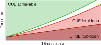
Figure 1: Achievability of CUE and CHSE in time $m$-quasiperiodic systems with quasienergy eigenstates. The red regions represent no-go theorems for CHSE and CUE presented in Sec. IV, for $m<2(d-1)$ (Theorem 1 and Theorem 2) and $m<d^{2}-d$ (Theorem 3), respectively. The green region represents an explicit construction of a $(m=d^{2}-2)$-quasiperiodic system with QEs that satisfies CUE, presented in Sec. V.

Our work represents a step towards a unified understanding of quantum ergodicity in generic time-dependent quantum systems. Our dynamical notion of ergodicity harmonizes with the notions in classical systems, and further provides a physical understanding of how thermalization arises in these systems, without reference to stationary states of dynamics.

This work is organized as follows. We begin by introducing the relevant concepts underlying our analysis. In Sec. II, we first introduce our dynamical notion of quantum ergodicity, CHSE and CUE, defined via the toolset of quantum state/unitary-designs. In Sec. III, we recap quasiperiodically-driven systems and their structure in dynamics and, in particular, a generalization of the Floquet decomposition into windings of quasienergies and quasienergy eigenstates on high-dimensional tori. The reader knowledgeable in these topics may elect to skip this section. In Sec. IV, we present our first results: three no-go theorems establishing conditions under which CUE and CHSE are physically impossible, when the number of frequencies driving the Hamiltonian are not sufficiently large, in relation to the dimension. In Sec. V, we demonstrate the converse: an explicit construction of a quasiperiodically driven system which satisfies CUE (and hence CHSE), with a sufficiently large number of driving frequencies. In Sec. VI, we consider relaxing ergodicity to comparing finite moments. We show that Floquet systems can achieve this relaxed notion of ergodicity by providing examples in both continuous and discrete time. Lastly, in Sec. VII, we close with a discussion of connections to previous works and future directions.

Before proceeding, let us remark that dynamical notions of quantum ergodicity have recently been discussed in other works [21, 22, 23, 24, 25]. By borrowing notions from classical ergodic theory, Ref. [21] provides a definition of quantum ergodicity that requires that certain basis vectors are cyclically transported to each other in a precise sense. Separately, Refs. [22, 23] build connections between temporal unitary designs and the ETH. Although the conservation of energy prevents the temporal ensemble from forming an exact $k$-design, these references relax the $k$-design condition in two distinct ways: Ref. [22] introduces a partial unitary design, which restricts to expectation values of some observables, while Ref. [23] uses free probability to construct a notion dubbed $k$-freeness. Common to these works is the focus on time-independent systems. In contrast, the stronger dynamical version of quantum ergodicity studied in our work requires the absence of any conserved quantity, and is suited for time-dependent systems without energy conservation. Bridging our work and these other notions of quantum ergodicity is an interesting question.

II Dynamical formulation of Quantum ergodicity

Consider a $d$-dimensional quantum system undergoing dynamics under a time-dependent Hamiltonian or a quantum circuit. An immediate question arises, which forms the fundamental motivation behind our work: is there a sense in which such a system can be termed ergodic?

In this section, we will introduce a concept of quantum ergodicity defined in terms of statistical similarities of temporal ensembles of dynamical objects — namely, time-evolved wavefunctions as well as time-evolution operators, to ensembles of such objects distributed unbiasedly (i.e., uniformly) in the respective spaces that they live in. In more pedestrian terms, this is the familiar idea of “time-averaging equals space-averaging” in classical dynamics, applied to the quantum setting.

II.1 Hilbert-space ergodicity (HSE)

We start by discussing quantum ergodicity at the level of quantum states $\ket{\psi(t)}=U(t)\ket{\psi(0)}$ uniformly covering the Hilbert space over time, a notion first introduced already in Ref. [7], dubbed “Complete Hilbert-Space Ergodicity” (CHSE). More precisely, since global phases are irrelevant, it was proposed to consider whether the ensemble of time-evolved density matrices $\{\psi(t)\}_{t\geq 0}$ called the ‘temporal ensemble’ (if it exists ), where $\psi(t)=|\psi(t)\rangle\langle\psi(t)|$, is statistically indistinguishable to the ensemble of states $\{\phi\}_{\text{Haar}}$ called the ‘spatial ensemble’. The latter is defined as the set of states randomly sampled without preference to a particular direction in the projective Hilbert-space $\mathbb{P}(\mathbb{C}^{d})=\{\psi=\outerproduct{\psi}{\psi}\,\colon\ket{\psi}\in\mathbb{C}^{d},\,\innerproduct{\psi}{\psi}=1\}$, or in other words, the set where states $\phi$ and $V\phi V^{\dagger}$ occur equally likely, where $V$ is drawn from the unique, uniform Haar measure on the space of unitaries [27]. Formally, we have:

Definition 1 (CHSE).

Complete Hilbert-space ergodicity (CHSE) [7] is the property of quantum dynamics wherein the temporal and spatial ensembles of quantum states are statistically indistinguishable for any initial state $\psi(0)\in\mathbb{P}(\mathbb{C}^{d})$, that is, $\{\psi(t)\}_{t\geq 0}\sim\{\phi\}_{\text{Haar}}$, where “$\sim$” denotes equality in distribution.

To make the comparison quantitative, we can consider finite moments of the respective distributions. For the temporal ensemble, the $k$-th moment is defined as:

$$\rho_{\mathrm{time}}^{(k)}:=\mathop{{}\mathbb{E}}_{t\geq 0}[{\psi(t)}^{\otimes k}]=\lim_{T\to\infty}\frac{1}{T}\int_{0}^{T}\differential{t}(U(t)\psi(0)U(t)^{\dagger})^{\otimes k},$$ (1)

which involves $k$ replicas of the time-evolved state, while the $k$-th moment of the spatial ensemble $\{\phi\}_{\text{Haar}}$ is defined as:

$$\rho^{(k)}_{\text{Haar}}:=\mathop{{}\mathbb{E}}_{\phi\in\mathbb{P}(\mathbb{C}^{d})}[{\phi}^{\otimes k}]=\int\differential{U}(U\phi_{0}U^{\dagger})^{\otimes k},$$ (2)

where $\differential{U}$ is the Haar measure on the unitary space and $\phi_{0}$ any fixed reference state. We note that $\rho^{(k)}_{\text{Haar}}$ have simple, closed-formed expressions as sums of permutation operators over the $k$-replicated Hilbert space [see Eq. (23)], which can be derived using Schur’s Lemma in representation theory [28]. As an example, $\rho^{(1)}_{\text{Haar}}=\mathds{1}/d$ is the maximally-entropic state, where $\mathds{1}$ is the identity operator on a single copy of the Hilbert space; while $\rho^{(2)}_{\text{Haar}}=(\mathds{1}+S)/d(d+1)$, where here $\mathds{1}$ $(S)$ is the identity (swap) operator on the tensor product of two Hilbert spaces. Using the $k$-th moments $\rho^{(k)}_{\text{Haar}}$, we can define a less restrictive notion of Hilbert-space ergodicity in terms of statistical indistinguishability of only up to $k$-moments:

Definition 2 ($k$-HSE).

A closed quantum system is said to exhibit Hilbert-space $k$-ergodicity ($k$-HSE), for $k\in\mathbb{N}$, if for any initial state $\psi(0)\in\mathbb{P}(\mathbb{C}^{d})$,

$$\rho_{\mathrm{time}}^{(k)}=\rho_{\mathrm{Haar}}^{(k)}.$$ (3)

Any standard matrix norm can be used to ascertain this equality (captured by vanishing of the norm of $\rho^{(k)}_{\text{time}}-\rho^{(k)}_{\text{Haar}}$), but it is conventional to use the trace distance $D(\rho,\sigma):=\frac{1}{2}\|\rho-\sigma\|_{1}$, where $\|\cdot\|_{1}$ is the trace norm, given by the sum of the absolute value of the eigenvalues. This is because $\rho_{\mathrm{time}}^{(k)}$ and $\rho_{\mathrm{Haar}}^{(k)}$ have interpretations of density operators on the $k$-replicated Hilbert space, and the trace norm operationally captures the probability of distinguishing these two states under an optimal measurement.

In the parlance of quantum information theory, $k$-HSE is the statement that the temporal ensemble forms a (state) $k$-design (see [29] and App. A). Note that $k$-HSE implies $k^{\prime}$-HSE for $k^{\prime}\leq k$ but not vice versa, and thus forms a hierarchical definition of more and more restricted notions of quantum ergodicity for higher $k$ (see Corollary A5 and Fig. 2). CHSE, which is at the top of this hierarchy, is then recovered by demanding equality for all $k$:

Definition 3 (CHSE; equivalent definition ).

If a system exhibits $k$-HSE for all $k$ for any initial state $\psi(0)\in\mathbb{P}(\mathbb{C}^{d})$, then it is said to exhibit complete Hilbert-space ergodicity (CHSE).

In terms of physical observables, $k$-HSE constrains the behavior of time-averaged expectation values $\tr(O^{(k)}\psi(t)^{\otimes k})$ of a joint observable $O^{(k)}$ on the $k$-replicated Hilbert space. In the case of a product observable $O^{(k)}=O^{\otimes k}$, this is the time-averaged $k$th power of $\expectationvalue{O}{\psi(t)}$. For example, $1$-HSE implies that the time average of $O$, given by $\mathop{{}\mathbb{E}}_{t\geq 0}[\langle\psi(t)|O|\psi(t)\rangle]=\lim_{T\to\infty}\frac{1}{T}\int_{0}^{T}dt\langle\psi(t)|O|\psi(t)\rangle$, equals $\mathop{{}\mathbb{E}}_{\phi\in\mathbb{P}(\mathbb{C}^{d})}[\expectationvalue{O}{\phi}]=\tr(O)/d$ regardless of the initial state $\psi(0)$, i.e., the system over long times reproduces expectation values within the infinite-temperature state. More generally, $k$-HSE implies $\mathop{{}\mathbb{E}}_{t\geq 0}[\langle\psi(t)|O|\psi(t)\rangle^{k}]=\lim_{T\to\infty}\frac{1}{T}\int_{0}^{T}dt\langle\psi(t)|O|\psi(t)\rangle^{k}$ is equal to $\mathop{{}\mathbb{E}}_{\phi\in\mathbb{P}(\mathbb{C}^{d})}[\expectationvalue{O}{\phi}^{k}]=\text{tr}({O}^{\otimes k}\rho^{(k)}_{\text{Haar}})$ , which is independent of $\psi(0)$ and can be calculated using the closed form expression of $\rho^{(k)}_{\text{Haar}}$ described above, which physically constrains not only the mean but also temporal fluctuations and beyond to mimic those computed for random states. For instance, for $k=2$, the spatial averaging yields explicitly $(\text{tr}(O^{2})+\text{tr}(O)^{2})/d(d+1)$. CHSE is the strongest statement that the time-average of any (analytic) function $f$ is equal to its spatial average, i.e., $\mathop{{}\mathbb{E}}_{t\geq 0}[f({\psi(t)})]=\mathop{{}\mathbb{E}}_{\phi\in\mathbb{P}(\mathbb{C}^{d})}[f({\phi})]$. This is the consequent of Birkhoff’s Ergodic Theorem [32], applied to a quantum system.

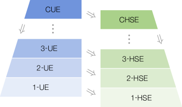
Figure 2: Dynamical notions of quantum ergodicity and their relations. Unitary $k$-ergodicity ($k$-UE) (left) and Hilbert-space $k$-ergodicity ($k$-HSE) (right), with complete unitary ergodicity (CUE) and complete Hilbert-space ergodicity (CHSE) on top, respectively. Arrows indicate logical implication.

II.2 Unitary ergodicity (UE)

We propose in this work to also consider a different notion of dynamical quantum ergodicity, captured by the equivalence of statistics of the ensemble of time-evolution operators $\{U(t)\}_{t\geq 0}$ to the uniform ensemble of operators in the space of unitaries. The evolution operators are given by the time-ordered exponentials $U(t)=\mathcal{T}\text{exp}(-i\int_{0}^{t}\differential{\tau}H(\tau))$ which propagate the system from time $0$ to time $t$. More precisely, it is natural to consider the set of unitary quantum channels $\{\mathcal{U}(t)\}_{t\geq 0}$, defined by $\mathcal{U}(t)[\psi]=U(t)[\psi]U(t)^{\dagger}$ (we consider channels as opposed to the unitary time-evolution operators themselves, as global phase information is irrelevant). For technical convenience, the map $\mathcal{U}(t)$ can be vectorized into the form $U(t)^{*}\otimes U(t)$. These are elements of the projective unitary group $\operatorname{PU}(d)=\{V^{*}\otimes V\,:\,V\in\operatorname{U}(d)\}$ for which there is a notion of a uniform (Haar) ensemble $\{\mathcal{V}\}_{\text{Haar}}:=\{V^{*}\otimes V\}$ describing the distribution of unitary channels obtained from randomly sampling from the Haar measure $dV$ on the space of unitaries [27]. Our proposed dynamical notion of quantum ergodicity in this scenario would then amount to asking whether the temporal ensemble is equivalent to the spatial ensemble, which in analogy to CHSE we dub “complete unitary ergodicity”:

Definition 4 (CUE).

Complete unitary ergodicity (CUE) is the property of quantum dynamics wherein the temporal ensemble of unitary time-evolution operators and spatial ensemble of unitary operators are statistically indistinguishable, $\{\mathcal{U}(t)\}_{t\geq 0}\sim\{\mathcal{V}\}_{\text{Haar}}$, where “$\sim$” denotes equality in distribution.

Such an equality may, once again, be probed by comparing moments of the respective distributions, defined for the $k$-th moment for the temporal ensemble as $\mathop{{}\mathbb{E}}_{t\geq 0}[U(t)^{\otimes k,k}]:=\lim_{T\to\infty}\frac{1}{T}\int_{0}^{T}dt(U(t)^{*}\otimes U(t))^{\otimes k}$, and for the spatial ensemble as $\mathop{{}\mathbb{E}}_{V\sim\mathrm{Haar}}[V^{\otimes k,k}]$, where ${V}^{\otimes k,k}:=(V^{*}\otimes V)^{\otimes k}$. The latter can be exactly computed using so-called Weingarten calculus and have closed form expressions [34]. For example, the first moment $\mathop{{}\mathbb{E}}_{V\sim\mathrm{Haar}}[{V^{*}\otimes V}]$ is equal to the quantum channel $\mathcal{C}^{(1)}[O]=\tr(O)\mathds{1}/d$, meaning that, under $1$-UE, the time-average of any observable $O(t)$ in the Heisenberg picture is $\mathop{{}\mathbb{E}}_{t\geq 0}[O(t)]=\tr(O)\mathds{1}/d$. We can then define $k$-unitary ergodicity as the statement of indistinguishability only up to the $k$-th moment:

Definition 5 (UE).

For $k\in\mathbb{N}$, we say that the evolution given by a Hamiltonian $H(t)$ exhibits unitary $k$-ergodicity ($k$-UE) if the evolution operator $U(t)$ satisfies

$$\mathop{{}\mathbb{E}}_{t\geq 0}[U(t)^{\otimes k,k}]=\mathop{{}\mathbb{E}}_{V\sim\mathrm{Haar}}[{V^{\otimes k,k}}].$$ (4)

Again, any vanishing of matrix norm for the difference between the left and right hand sides can be used to numerically ascertain $k$-UE, though it is common practice to compare the so-called “frame-potentials” (which is related to the Frobenius norm), viz asking if

$$\mathop{{}\mathbb{E}}_{t\geq 0}\mathop{{}\mathbb{E}}_{t^{\prime}\geq 0}\Big{[}\absolutevalue{\tr(U^{\dagger}(t^{\prime})U(t))}^{k}\Big{]}\stackrel{{\scriptstyle?}}{{=}}\mathop{{}\mathbb{E}}_{V,W\sim\mathrm{Haar}}\Big{[}\absolutevalue{\tr(W^{\dagger}V)}^{2k}\Big{]}.$$ (5)

In the parlance of quantum information theory, $k$-UE is the statement that the temporal ensemble forms a unitary $k$-design.

It is straightforward to note that $k$-UE implies $k$-HSE, but the converse is not true (see App. A). Thus, $k$-UE is an inequivalent, strictly stronger version of quantum ergodicity compared to $k$-HSE. Further, $k$-UE defines a hierarchical definition of more restricted notions of quantum ergodicity: $k$-UE implies $k^{\prime}$-UE for $k^{\prime}\leq k$ but not vice versa (see Corollary A5 and Fig. 2). The most restrictive condition is when $k$-UE is satisfied for all $k$, leading us back to CUE:

Definition 6 (CUE; equivalent definition).

If a system exhibits $k$-UE for all $k$, then it exhibits complete unitary ergodicity (CUE).

Similarly to $k$-UE and $k$-HSE, CUE implies CHSE but not vice versa.

II.3 Achievability of HSE or UE and conservation laws

We briefly comment here on the achievability of HSE or UE in the presence of conservation laws in dynamics. As the definition of HSE or UE entails a comparison of the temporal ensemble to the reference uniform (i.e., unbiased) distribution in the Hilbert space/space of unitaries, it is intuitively clear that any conserved quantities will preclude HSE/UE, since there will be “bias” in dynamics towards them (of course, an interesting question, which we do not address here, is how to properly modify the reference distribution in order to account for conserved quantities [25]). For example, in a time-independent quantum system which has energy conservation, not even $1$-HSE can be achieved: if $\ket{\psi}$ is an eigenstate of the Hamiltonian, then its time average remains pure: $\psi=\mathop{{}\mathbb{E}}_{t\geq 0}[\psi(t)]$, far off from a maximally mixed state $\mathop{{}\mathbb{E}}_{\phi\in\mathbb{P}(\mathbb{C}^{d})}[\phi]=\mathds{1}/d$.

Achieving quantum ergodicity defined by HSE or UE therefore necessarily requires considering systems with time-dependence, such that there are no conservation laws. A trivial example of dynamics which satisfies CUE is a drive $U(t)$ where at every integer time $t$ an independent Haar random unitary is applied. Then, the wavefunction undergoes a random walk in the Hilbert space. The time dependence of such a drive is, however, maximally complex: at each time-step we need to specify a completely new random matrix. A natural question to ask is whether or not CHSE/CUE (or more generally different levels of the hierarchy of complete ergodicity) can be achieved with time-dependent systems with more succinct, deterministic, descriptions. Surprisingly, Ref. [7] gave an explicit example in the affirmative, in terms of a family of simple, deterministic, low-complexity quantum drives, derived from the Fibonacci word and its variants, which provably exhibits CUE (and hence CHSE). However, a more general theory that allows to systematically determine when CUE or CHSE occurs or not, is at the present time still not fully established. One of the aims of this work is to present a step in this direction.

In the next section, we introduce the notion of time-quasiperiodicity, which allows to classify the time dependence of a system in increasing levels of complexity. Using this, we will systematically classify the time-complexity required to achieve the different levels of HSE and UE in the class of quasiperiodically driven systems.

III Time-quasiperiodic quantum systems

In this section, we give a brief introduction to the class of quantum systems which are quasiperiodically-driven by $m$ frequencies, and discuss the structure of the dynamics they generate; in particular, the possibility of decomposing dynamics into quasienergies and quasienergy states.

Time-quasiperiodic systems are the direct generalization of a Floquet system, i.e., a system driven periodically by a single fundamental frequency [8, 9, 10, 11, 12, 13, 14, 15, 16]. This class of systems has gained much recent interest [35, 36, 37, 38, 39, 40], as they may host novel and exotic dynamical phases like time-quasiperiodic topological phases [41, 42, 43] and time quasi-crystals [44, 45, 46, 47, 48].

III.1 Definition

Floquet Hamiltonians are those that periodically repeat themselves in time, $H(t)=H(t+T)$, where $\omega$ is the fundamental driving frequency and $T=2\pi/\omega$ the corresponding period. An equivalent way of understanding such Hamiltonians, which allows for an immediate generalization to multi-frequency drives, is to define an underlying Hamiltonian $\hat{H}(\theta)$ on the circle $\mathbb{S}^{1}$, with coordinate $\theta\in[0,2\pi)$. Then, a time-periodic Hamiltonian can be defined via setting $\theta=\omega t+\theta_{0}\mod 2\pi$ for some initial phase $\theta_{0}$ (which we will typically set to be 0), i.e., $H(t)=\hat{H}(\omega t)$. A multi-tone, or time-quasiperiodic Hamiltonian then straightforwardly follows by generalizing this concept, by promoting the circle $\mathbb{S}^{1}$ to the torus $\mathbb{T}^{m}=\underbrace{\mathbb{S}^{1}\times\mathbb{S}^{1}\times\cdots\times\mathbb{S}^{1}}_{m\text{ times}}\ni\bm{\theta}=(\theta_{1},\dots,\theta_{m})$, and $\omega$ to $\bm{\omega}=(\omega_{1},\dots,\omega_{m})$. Precisely, we have:

Definition 7 ($m$-time-quasiperiodic Hamiltonian).

Given a Hamiltonian $H(t)$, with $t\in\mathbb{R}$, we say that $H$ is time-quasiperiodic with $m$ tones, or $m$-time-quasiperiodic if there exists a so-called parent Hamiltonian $\hat{H}(\bm{\theta})$ piecewise-smoothly defined on the $m$-dimensional torus $\mathbb{T}^{m}\coloneqq\{\bm{\theta}=(\theta_{1},\dots,\theta_{m})\,|\,\theta_{j}\in[0,2\pi)\}$ such that

$$H(t)={\hat{H}}(\bm{\omega}t),$$ (6)

for some frequency vector $\bm{\omega}=(\omega_{1},\dots,\omega_{m})$, where the winding $\bm{\omega}t$ is taken modulo $2\pi$ at each entry. Furthermore, we require that $m$ is the smallest integer such that the above decomposition holds.

As $m$ has to be the smallest possible number of tones, the frequency vector $\bm{\omega}$ has to be rationally independent, meaning that the only integer solution $\bm{n}\in\mathbb{Z}^{m}$ to the equation $\bm{n}\cdot\bm{\omega}=0$ is $\bm{n}=\bm{0}$, i.e., $\bm{\omega}$ constitute $m$ independent fundamental tones . Henceforth, for simplicity in the notation, we will drop the hat in the parent Hamiltonian $\hat{H}(\bm{\theta})$, and simply write $H(\bm{\theta})$. This is a standard abuse of notation, as $H(t)$ and $H(\bm{\theta})$ are functions technically defined in different domains, but they can easily be distinguished by their arguments [43]. A more familiar definition of an $m$-time-quasiperiodic Hamiltonian, which is equivalent for sufficiently well-behaved functions, is the statement that $H(t)$ can be written as a convergent Fourier series with $m$ rationally-independent fundamental frequencies,

$$H(t)=\sum_{\bm{n}\in\mathbb{Z}^{m}}{H}_{\bm{n}}e^{i\bm{n}\cdot\bm{\omega}t},$$ (7)

where $H_{\bm{n}}$ are its Fourier modes (over the torus).

More generally, an $m$-time-quasiperiodic Hamiltonian constitutes an example of an $m$-time-quasiperiodic function $F(t)=\hat{F}(\bm{\omega}t)=\sum_{\bm{n}\in\mathbb{Z}^{m}}{F}_{\bm{n}}e^{i\bm{n}\cdot\bm{\omega}t}$, where the parent function $\hat{F}$ and frequency vector $\bm{\omega}$ have all the same properties as that listed in Definition 7.

III.2 Generalized Floquet decomposition

What is understood about the nature of quantum dynamics generated by time-quasiperiodic Hamiltonians? In the case of $m=1$, we recover time-periodic or Floquet drives, for which the Floquet theorem guarantees that there exists a set of quasienergy eigenstates which are also periodic in time [51]. This is captured by the statement that the unitary time-evolution operator admits a decomposition

$$U(t)=P(\omega t)e^{-iQt},$$ (8)

where $Q$ is the so-called Floquet Hamiltonian whose $d$ eigenvalues, called quasienergies, and eigenvectors are defined via $Q|\alpha\rangle=q_{\alpha}|\alpha\rangle$. $P(\omega t)$ is a periodic unitary with identical period as the driving Hamiltonian and satisfies $P(0)=\mathds{1}$, and thus is descended from a piecewise-smooth parent unitary $P(\theta)$ defined on the circle $\mathbb{S}^{1}$. One may thus construct quasienergy eigenstates (QE) that live on the circle, defined via

$$|\alpha(\theta)\rangle=P(\theta)|\alpha\rangle.$$ (9)

Note that the decomposition into the Floquet Hamiltonian and periodic unitary is not unique: one can shift the quasienergies $q_{\alpha}+n\omega$ by any integer $n\in\mathbb{Z}$ and redefine the appropriate component of $P(\omega t)$ with a winding phase. One sees from this decomposition that if we were to view a Floquet system at stroboscopic times $t=nT$ where $n\in\mathbb{Z}$, then the system can equivalently be thought of as undergoing dynamics under a time-independent Hamiltonian $Q$, that is, $U(nT)=e^{-iQnT}$. This property of decomposability of dynamics into that of a static Hamiltonian, up to a periodic envelop, is known mathematically as reducibility [52, 53].

When $m>1$, it is natural to assume that a generalized Floquet decomposition, or reducibility of dynamics, holds too, namely that

$$U(t)=P(\bm{\omega}t)e^{-iQt},$$ (10)

where $P(\bm{\theta})$ is a piecewise-smooth unitary defined on $\mathbb{T}^{m}$ which satisfies $P(\bm{0})=\mathds{1}$ , and $Q$ is the generalized Floquet Hamiltonian with $d$ quasienergies and eigenstates, $Q\ket{\alpha}=q_{\alpha}\ket{\alpha}$. Similar to the Floquet case, the generalized Floquet Hamiltonian $H_{F}$ and unitary $P(\bm{\theta})$ will not be unique, but this fact will be unimportant in our analysis. One may then construct quasienergy eigenstates (QEs), now defined as state-valued functions on the torus,

$$\ket{\alpha(\bm{\theta})}=P(\bm{\theta})\ket{\alpha}.$$

Such a decomposition would then entail that if we prepare our system in the initial state $\ket{\alpha}=\ket{\alpha({\bm{0}})}$, the resulting dynamics is $m$-time-quasiperiodic up to a global phase:

$$\ket{\alpha(t)}=U(t)\ket{\alpha}=e^{-iq_{\alpha}t}\ket{\alpha(\bm{\theta}=\bm{\omega}t)}.$$

More generally, the time dependence of a generic initial state may then be decomposed as a linear combination over QEs:

$$\ket{\psi(t)}=\sum_{\alpha}c_{\alpha}e^{-iq_{\alpha}t}\ket{\alpha(\bm{\omega}t)},$$ (11)

with $c_{\alpha}=\innerproduct{\alpha}{\psi(0)}$, which can be understood as time-quasiperiodic over the torus $\mathbb{T}^{n}$, with $n\leq(m+d-1)$ (ignoring the global phase). The factor of $m$ comes from the physical driving frequencies $\bm{\omega}$, while there are $d$ additional frequencies coming from the winding phases $e^{-iq_{\alpha}t}$, minus a global phase.

As appealing as the generalized Floquet decomposition Eq. (10) is, we stress its existence is nontrivial: it is known rigorously that this may not always hold in $(m>1)$-time-quasiperiodic systems [17, 18]. This could come for example from topological obstructions in defining a smooth quasienergy state over the torus, see [42]. In other words, a generalized Floquet theorem (i.e., applying to all time-quasiperiodic Hamiltonians) does not hold, though the Floquet decomposition may still be valid in some cases. However, while interesting in its own right, the purpose of this work is not to investigate the conditions for when such a decomposition does or does not hold in time-quasiperiodic systems; rather, we assume that the systems in consideration always admit generalized QEs and study the compatibility of HSE/UE with such structure in dynamics. Note that the existence of QEs guarantees that the infinite-time averages in Eq. (3) [Eq. (4)] always exist, i.e., the temporal ensemble of states/unitaries is well-defined in the limit $t\to\infty$ .

IV Quasienergy eigenstates limit complete quantum ergodicity

Having introduced the concepts of Hilbert-space ergodicity and unitary ergodicity, and the class of quantum dynamics (time-quasiperiodic systems) we consider in this paper, we are now in a position to present our results. Our first finding shows that the existence of QEs in time-periodic ($m=1$) systems precludes them from satisfying CHSE (and hence CUE). That is, Floquet systems cannot achieve full dynamical quantum ergodicity.

Theorem 1.

If $H(t)$ is a time-periodic Hamiltonian with period $T$ and a bounded strength in a sense that ${B=\int_{0}^{T}\differential{t}\norm{H(t)}_{\infty}<\infty}$ , then $H(t)$ does not exhibit CHSE (and thus not CUE).

The quantity $B$ should be understood as a measure of the “physical resources” needed to realize the dynamics: it is large for Hamiltonians whose strengths $\|H(t)\|_{\infty}$ are large or whose driving period is long. Although $B$ changes upon the substitution $H(t)\rightarrow H(t)+c(t)\mathds{1}$, its minimum value over all $c(t)$ is proportional to the time-integrated bandwidth $B=\tfrac{1}{2}\int_{0}^{T}\differential{t}(E_{\max}(t)-E_{\min}(t))$ . As $B$ carries units of energy $\times$ time (recall $\hbar=1$), it has also the meaning of an “action”, which physically corresponds to the net effect that $H(t)$ has on the system during a single driving period. As we explain further below, $B<\infty$ is simply the physical requirement of a “quantum speed limit”: that the length of the trajectory traversed by the wavefunction over a period $T$ cannot be arbitrarily long.

From this point of view, the logic behind the proof of Theorem 1 can be intuitively explained as an incompatibility of dynamics that traverses a finite “distance” to densely cover the continuous space that is the Hilbert space. Indeed, the formal proof proceeds by contradiction:

Proof.

Assume that the time-periodic Hamiltonian $H(t)$ satisfies CHSE. By Floquet’s theorem, $H(t)$ has a QE $\ket{\alpha(t)}=e^{-iq_{\alpha}t}\ket{\alpha(\theta=\omega t)}$, where $\omega=2\pi/T$. Because phases are projected out in $\mathbb{P}(\mathbb{C}^{d})$, dynamics beginning from $\alpha(0)$ is time-periodic: $\alpha(t)=\alpha(\theta=\omega t)$. We will reach a contradiction, in three steps.

First, CHSE implies that the state $\alpha(t)$ uniformly visits the $2(d-1)$-dimensional projective Hilbert space $\mathbb{P}(\mathbb{C}^{d})$. This implies that the map $\theta\mapsto\alpha(\theta)$ is topologically dense, meaning that for any other state $\ket{\phi}$ and arbitrarily small $\varepsilon>0$ there is some angle $\theta$ for which $D(\alpha(\theta),\phi)<\varepsilon$, where

$$D(\psi,\phi)=\tfrac{1}{2}\norm{\psi-\phi}_{1}=\sqrt{1-\absolutevalue{\innerproduct{\psi}{\phi}}^{2}}$$ (12)

is the trace distance. This is rigorously proven in App. B.

Second, we appeal to the quantum speed limit $B<\infty$: the state $\alpha(t)$ can only travel through a finite path in $\mathbb{P}(\mathbb{C}^{d})$. Specifically, for any finite partition of the circle $\theta_{0}\leq\theta_{1}\leq\cdots\leq\theta_{n}=\theta_{0}+2\pi$,

$$\sum_{j=1}^{n}D(\alpha(\theta_{j-1}),\alpha(\theta_{j}))\leq B.$$ (13)

This is a state-independent variant of the quantum speed limit, which is traditionally phrased in terms of the average energy [59] or variance [60] of a specific state, rather than the Hamiltonian norm [61, 62]. Equation (13) is a straightforward consequence of Schrödinger’s equation (see App. C).

In our final step, we note that the previous two observations are contradictory: by dimensionality arguments, we can find $n\sim\delta^{-2(d-1)}$ different states $\phi_{1},\dots\phi_{n}$ pairwise separated by at least trace-distance $\delta$, i.e., $D(\phi_{i},\phi_{j})\geq\delta$ for $i\neq j$. If the trajectory $\alpha(\theta)$ is dense, at some angles $\theta_{1},\dots,\theta_{n}$ it must come $\varepsilon$-close to these states, $D(\alpha(\theta_{i}),\phi_{i})\leq\varepsilon$. From Eq. (13) and the triangle inequality we obtain $B\geq\delta^{-2(d-1)}(\delta-2\varepsilon)$, which can be made arbitrarily large by choosing small enough $\varepsilon$ and $\delta$, contradicting the finiteness of $B$. Full details are given in Proposition D16.

This shows the impossibility of CHSE. Lastly, because CHSE implies CUE, then CUE is also not achievable by time-periodic systems. ∎

In App. D we show a stronger form of Theorem 1. We prove that if a periodic Hamiltonian satisfies $k$-HSE for some finite $k$, then $B\coloneqq\int_{0}^{T}\differential{t}\norm{H(t)}_{\infty}$ is lower bounded as

$$B\geq\max\Big{\{}\frac{\sqrt{2}}{3k} \Bigg{(}\binom{k+d-1}{k}-1\Bigg{)},$$ (14)

$$\quad\frac{8}{(4d)^{d}}\left(\frac{k}{\log(k+1)}\right)^{d-\frac{3}{2}}\Big{\}}.$$

Informally, Eq. (14) says that time-periodic $k$-HSE is not achievable for large $k$ or $d$ unless the wavefunction travels for a very long distance within a single Floquet period $T$, in line with our physical intuition. For example, inserting $k=1$ in the first expression in the maximum, we see that $B\geq\frac{\sqrt{2}}{3}(d-1)$, where the linear growth with $d$ is required for a quasienergy eigenstate to come close to $d$ orthogonal states and achieve ${1}$-HSE. In general, for fixed $k$, $B(d)$ has to grow at least as $d^{k}$. For fixed $d$, $B(k)$ has to grow at least like ${(k/\log(k+1))^{d-\frac{3}{2}}}$, by the second expression in Eq. (14), which is obtained from analyzing the geometrical distribution of a $k$-design in $\mathbb{P}(\mathbb{C}^{d})$. In Sec. VI, we provide explicit examples of time-periodic quantum systems with $B$ large enough such that $k$-HSE is provably achievable.

Our next result is a generalization of Theorem 1 to $m$-time-quasiperiodic Hamiltonians, where we remind the reader our analysis is under the premise of the existence of QEs. Like in the Floquet case $(m=1)$, such QEs can lead to an obstruction of the system to achieve CHSE/CUE: dynamics beginning from a QE is necessarily structured — specifically time-quasiperiodic, or in other words, amounts to winding around an $m$-dimensional torus $\mathbb{T}^{m}$. It may then be possible this regularity precludes an unbiased exploration of the Hilbert space. However, unlike the Floquet case, now there is an interplay between the number of tones $m$ of the drive (its “complexity”), and the dimension $d$ of the ambient space: such obstruction is only active if the torus is small enough, such that the time-evolved state is unable to fully “wrap” around the projective Hilbert space. Indeed, we have, from a counting-of-dimensions argument:

Theorem 2.

Let $H(t)$ be a $m$-quasiperiodic Hamiltonian with a piecewise smooth quasienergy eigenstate. Then $H(t)$ cannot exhibit CHSE if

$$m<2(d-1).$$ (15)

Proof.

The quasienergy eigenstate $\alpha(t)$ densely visits $\mathbb{P}(\mathbb{C}^{d})$ in time (see App. B). By the quasiperiodicity of the time evolution, $\alpha(t)=\alpha(\bm{\theta}=\bm{\omega}t)$, we deduce that the map $\bm{\theta}\mapsto\alpha(\bm{\theta})$ is dense, from $\mathbb{T}^{m}$ to $\mathbb{P}(\mathbb{C}^{d})$. Because $\bm{\theta}\mapsto\alpha(\bm{\theta})$ is piecewise continuous, this map must be surjective, or entirely covering $\mathbb{P}(\mathbb{C}^{d})$. Intuition suggests that a surjective map from $\mathbb{T}^{m}$ to $\mathbb{P}(\mathbb{C}^{d})$ requires that the dimension of the codomain, $\text{dim}(\mathbb{P}(\mathbb{C}^{d}))=2(d-1)$ (the amount of real numbers required to specify a pure density matrix), is not greater than the dimension of the domain $m=\text{dim}(\mathbb{T}^{m})$. This intuition is correct, as long as the map $\bm{\theta}\mapsto\alpha(\bm{\theta})$ is piecewise smooth in the torus, which is required in our definition of quasienergy eigenstate . The technical reason is that a piecewise smooth map is piecewise Lipschitz-continuous, and such maps do not increase Hausdorff dimension [64, 1.7.19]. Thus, CHSE requires $m\geq 2(d-1)$. ∎

The bound $m<O(d)$ where CHSE is impossible is obtained from the real dimension of $\mathbb{P}(\mathbb{C}^{d})$. Similarly, the same idea can be applied for the consideration of CUE, and we will obtain a bound which is $m<O(d^{2})$, coming from the dimension of the projective unitary group.

Theorem 3.

Let $H(t)$ be an $m$-quasiperiodic Hamiltonian with a basis of piecewise smooth quasienergy eigenstates. Then the evolution given by $H(t)$ cannot exhibit CUE if

$$m<d(d-1).$$ (16)

We leave the detailed proof in App. E. The idea is to note that the generalized Floquet decomposition for $U(t)=P(\bm{\omega}t)e^{-iQt}$ is quasiperiodic, with $m$ tones corresponding to $P(\bm{\omega}t)$, and (at most) an extra $d-1$ tones corresponding to the winding phases $e^{-iQt}$, which then implies that $m+d-1=\dim(\mathbb{T}^{m+d-1})\geq\dim(\operatorname{PU}(d))=d^{2}-1$.

These three no-go theorems are depicted in Fig. 1.

V Many driving frequencies permit complete quantum ergodicity

In the previous section, we have identified constraints on a $m$-time-quasiperiodic Hamiltonian’s ability to uniformly cover either the Hilbert space (Theorem 2) or unitary space (Theorem 3), under the assumption of existence of QEs. They tell us that a quantum system driven with too few tones cannot exhibit dynamical ergodicity, namely, if $m<O(d)$, CHSE is impossible; while if $m<O(d^{2})$, CUE is impossible. Physically, this is sensible, as when the number of driving frequencies $m$ is small, dynamics will not be “complex” enough. However, this leaves open the obvious converse question: suppose $m$ is large enough. Then are there time-quasiperiodic systems that do exhibit CHSE/CUE?

In this section, we will answer this in the affirmative. We show how to construct explicit $m$-quasiperiodic Hamiltonians with $m=d^{2}-2$ tones that host QEs, and which provably satisfy CUE (and thus CHSE). Together with the no-go theorems of the previous section, this leads us to the “phase diagram” depicted in Fig. 1.

V.1 Single-qubit complete unitary ergodicity with $m=2$ driving frequencies

We start with the case for a single qubit, with $m=2$, which will motivate the generalization for systems of arbitrary dimension.

Our key idea is to construct states $\ket{\alpha(\bm{\theta})}$ ($\alpha=0,1$), parameterized by $\bm{\theta}=(\theta_{1},\theta_{2})$, that satisfy the CHSE condition, and then reverse-engineer a Hamiltonian which has these states as its quasienergy eigenstates. By imposing Eq. (3) on the states $\ket{\alpha(\bm{\theta})}$, for all $k$, the resulting Hamiltonian will satisfy CHSE, but further CUE, which will motivate the generalization to $d>2$.

The CHSE condition requires the state $\alpha(t)=\outerproduct{\alpha(t)}{\alpha(t)}$ to uniformly cover the Bloch sphere $\mathbb{P}(\mathbb{C}^{2})$. Because $\alpha(t)=\alpha(\bm{\theta}=\bm{\omega}t)$, we can achieve this by selecting $\bm{\omega}=(\omega_{1},\omega_{2})$ to be rationally independent, and ${\alpha(\bm{\theta})}$ to be uniformly distributed on $\mathbb{P}(\mathbb{C}^{2})$, as a function of the angles $\bm{\theta}$ on the torus $\mathbb{T}^{2}$.

First, we construct the state $\ket{0({\bm{\theta}})}$, parameterized as

$$\ket{0(\bm{\theta})}=\sqrt{p(\theta_{1})}\ket{0}+\sqrt{1-p(\theta_{1})}e^{-i\theta_{2}}\ket{1}.$$

To uniformly cover the Bloch sphere, the function $p(\theta_{1})$ needs to be uniformly distributed in $[0,1]$ when $\theta_{1}$ is uniformly distributed in $[0,2\pi)$. This is achieved by any surjective function such that $\absolutevalue*{\tfrac{\differential p}{\differential\theta_{1}}}$ is almost-everywhere constant. Here, we consider $p(\theta_{1})=\absolutevalue{1-\theta_{1}/\pi},$ which is continuous on the circle. The resulting map is depicted in Fig. 3.

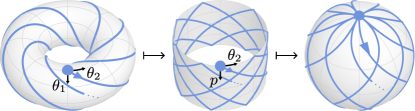
Figure 3: Transformation ${\bm{\theta}}\mapsto\ket{0(\bm{\theta})}$. A pair of angles $\bm{\theta}=(\theta_{1},\theta_{2})$ in the torus (left) is mapped to $(p(\theta_{1}),\theta_{2})$ in the cylinder (middle), which is further mapped to the state $\ket{0(\bm{\theta})}=\sqrt{p}\ket{0}+e^{-i\theta_{2}}\sqrt{1-p}\ket{1}$ in the Bloch sphere (right). The blue line displays time evolution $\bm{\theta}=\bm{\omega}t$, with a blue disk marking $t=0$.

Having defined $\ket{0(\bm{\theta})}$, we set $\ket{1(\bm{\theta})}$ to be the orthogonal state

$$\ket{1(\bm{\theta})}=\sqrt{p(\theta_{1})}\ket{1}-\sqrt{1-p(\theta_{1})}e^{i\theta_{2}}\ket{0}.$$

We now use these two states to construct a quasiperiodic Hamiltonian which has them as QEs. We can write these two states as the columns of a unitary $P(\bm{\theta})$, (i.e., $\ket{\alpha(\bm{\theta})}=P(\bm{\theta})\ket{\alpha}$), where

$$P(\theta_{1},\theta_{2})=\begin{pmatrix}\cos\xi(\theta_{1})&&-\sin\xi(\theta_{1})e^{i\theta_{2}}\\ \sin\xi(\theta_{1})e^{-i\theta_{2}}&&\cos\xi(\theta_{1})\end{pmatrix},$$ (17)

and $\xi(\theta_{1})=\arccos\sqrt{p(\theta_{1})}$. Then we choose any rationally independent driving frequencies $\bm{\omega}=(\omega_{1},\omega_{2})$ and quasienergy $q$ to define the evolution operator to be given by the generalized Floquet decomposition, Eq. (10), substituting $Q=\text{diag}(-q,q)$, $\theta_{1}=\omega_{1}t$, and $\theta_{2}=\omega_{2}t$,

$$U(t)=\begin{pmatrix}\cos\xi(\omega_{1}t)e^{iqt}&&-\sin\xi(\omega_{1}t)e^{i(\omega_{2}-q)t}\\ \sin\xi(\omega_{1}t)e^{-i(\omega_{2}-q)t}&&\cos\xi(\omega_{1}t)e^{-iqt}\end{pmatrix}.$$ (18)

Finally, we can obtain the $2$-quasiperiodic Hamiltonian by the Schrödinger Equation $H(t)=i(\partial_{t}U(t))U(t)^{\dagger}.$

It turns out that the evolution given by Eq. (18) not only satisfies CHSE, but the stronger CUE. This is because the transformation

$$(\xi,\eta,\varphi)\mapsto\begin{pmatrix}\cos\xi\,e^{i\eta}&&-\sin\xi\,e^{i\varphi}\\ \sin\xi\,e^{-i\varphi}&&\cos\xi\,e^{-i\eta}\end{pmatrix}$$ (19)

is precisely the Euler-angle parametrization of the group $\operatorname{SU}(2)$, and furthermore the assignment $\xi=\arccos\sqrt{p(\theta_{1})}$ makes it measure preserving, i.e. maps the Haar measure of the torus $\mathbb{T}^{3}\ni(\theta_{1},\eta,\varphi)$ to the Haar measure of $\operatorname{SU}(2)$. Thus, upon substituting

$$\xi=\arccos\sqrt{\absolutevalue{1-\omega_{1}t/\pi}}, \eta=qt, \varphi=(\omega_{2}-q)t,$$ (20)

we guarantee that $U(t)$, in time, explores $\operatorname{SU}(2)$ uniformly.

In the next section, we explain how to generalize this construction to $\operatorname{SU}(d)$, to obtain a $d$-dimensional quasiperiodic Hamiltonian which has QEs and satisfies CUE. That is, the time evolution operator uniformly explores the entire $\operatorname{SU}(d)$ space (the projective unitary space acting on a qudit of dimension $d$) over time.

V.2 Qudit complete unitary ergodicity with $m=d^{2}-2$ driving frequencies

By considering a specific sequence of rotations of the form

$$R_{j}(\xi,\varphi,\eta)=\begin{pmatrix}\mathds{1}_{j-1}&&&\\ &\cos\xi e^{i\eta}&-\sin\xi e^{i\varphi}&\\ &\sin\xi e^{-i\varphi}&\cos\xi e^{-i\eta}&\\ &&&\mathds{1}_{d-j-1}\end{pmatrix},$$

one can construct Hurwitz’s parametrization of $\operatorname{SU}(d)$, in terms of $d^{2}-1$ Euler angles [65, 66, 67]. We utilize this parametrization to construct a $m$-quasiperiodic drive which satisfies CUE and has QEs, with $m=d^{2}-2$. This is done by explicitly defining the evolution operator $U(t)$ in the generalized Floquet decomposition form [Eq. (10)]. By assigning each Euler angle to a function of the driving frequencies and the quasienergies, we guarantee that $U(t)$ uniformly explores $\operatorname{SU}(d)$ in time. The assignment for the Euler angles is a generalization of Eq. (20), where the $d^{2}-1$ Euler angles are written in terms of the $m=d^{2}-2$ driving angles $\omega_{1}t,\dots,\omega_{m}t$, and one of the quasienergies. The details of this construction are left to App. F.

In our construction, only one quasienergy is related to one of the Euler angles, and the remaining quasienergy degrees of freedom are just averaged out in time. We leave as an open question if it is possible to utilize all the $d-1$ quasienergy degrees of freedom. If the answer is positive, this would decrease the required number of driving angles to $m=d^{2}-d$, saturating the bound given by Theorem 3 and removing the white sliver in the phase diagram in Fig. 1. If the answer is negative, then the bound in Theorem 3 could potentially be strengthened.

VI Quantum $k$-ergodicity in time-periodic systems

Theorems 1, 2, and 3 show that the existence of quasienergy eigenstates forbids the achievability of the most stringent forms of dynamical ergodicity: CHSE and CUE. It is natural to ask if there are similar obstructions to quantum ergodicity if one relaxes to finite moments, as in the notions of $k$-HSE and $k$-UE, introduced in Sec. II. Surprisingly, we show here that $k$-HSE and $k$-UE can be reached even by time-periodic Hamiltonians, corresponding to the minimal $m=1$ time-periodic or Floquet case.

The achievability of finite $k$-UE in time-periodic systems can be understood from the existence of finite $k$-unitary designs in quantum information theory [68, 69] — an ensemble of a finite number of unitaries which reproduces the Haar measure up to the $k$-th statistical moment (see App. A for more details).

Utilizing the fact that finite unitary $k$-designs exist, we may construct a periodic sequence of rotations which satisfies $k$-UE, over discrete time. The construction proceeds as follows: for any $k$, let $\mathcal{D}_{k}=\{V_{0},V_{1},\dots,V_{n-1}\}$ be a finite unitary $k$-design with $n$ elements, which can be selected so that $V_{0}=\mathds{1}$ by otherwise applying $V_{0}^{\dagger}$ to all of its elements. We define a periodic drive by applying a sequence of gates such that the evolution operator cycles through $\mathcal{D}_{k}$.

At time every integer time $t=j\mod n$, we apply the unitary $V_{j}V_{j-1}^{\dagger}$. Then, the evolution operator satisfies $U(t)=V_{j}$. In this case, the integral in the left-hand side of Eq. (4) which defines $k$-UE, can be rewritten in terms of the series

$$\lim_{N\to\infty}\frac{1}{N+1}\sum_{t=0}^{N}U(t)^{\otimes k,k}=\mathop{{}\mathbb{E}}_{\mathrm{Haar}}[{W^{\otimes k,k}}].$$

Note that this evolution has period $T=n$, and it can achieve the $k$-UE condition with $B={\int_{0}^{T}dt\|H(t)\|_{\infty}\leq n\pi}$, where the time-periodic Hamiltonian $H(t)$ consists of a sequence of infinite-strength kicks $H_{j}(t)=i\delta(t-j)\mathrm{log}(V_{j}V_{j-1}^{\dagger})$ which satisfy $\int dt\|H_{j}(t)\|_{\infty}\leq\pi$. This is consistent with the bound on $B$ given by Eq. (14), as $n$ has to be sufficiently large in order for $\mathcal{D}_{k}$ to form a unitary $k$-design.

In the construction above $k$-UE is achieved by a periodic sequence of gates, in discrete time. The Hamiltonian discontinuously drives the state around $\mathbb{P}(\mathbb{C}^{d})$. It is, however, interesting to ask if the same level of ergodicity can be achieved when the evolution is continuous, or even smooth. In what is left of this section, we present some examples to show that the answer is positive.

We provide examples of continuous time-periodic systems that satisfy $k$-HSE and $k$-UE. We start with a qubit, $d=2$. In this case, $k$-UE is completely characterized by the time trajectory of a single quasienergy eigenstate since the trajectory of the remaining state is determined by their orthogonality. In a single-qubit Hamiltonian $H(t)$, if one quasienergy eigenstate $\ket{\alpha(\theta)}$ ($\alpha=0$ or $\alpha=1$) satisfies the $k$-HSE condition

$$\mathop{{}\mathbb{E}}_{\theta\in\mathbb{T}}[\alpha(\theta)^{\otimes k}]=\mathop{{}\mathbb{E}}_{\phi\in\mathbb{P}(\mathbb{C}^{2})}[\phi^{\otimes k}],$$ (21)

and the corresponding quasienergy and driving frequency are rationally independent, then $H(t)$ satisfies $k$-UE (see Corollary G19). Thus, constructing a single-qubit time-periodic drive which satisfies $k$-UE reduces to designing a closed curve $\alpha(\theta)$ in $\mathbb{P}(\mathbb{C}^{2})$ which satisfies Eq. (21), from which one can construct the evolution operator by the Floquet decomposition $U(t)=P(\omega t)e^{-i\text{diag}(-q,q)}$ with $P(\theta)=\sum_{\alpha=0}^{1}\outerproduct{\alpha(\theta)}{\alpha}$, where $q,\omega$ are chosen to be rationally independent.

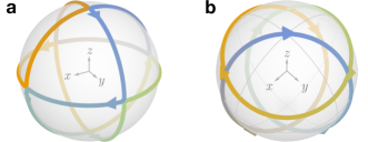
Figure 4: Single-qubit quasienergy eigenstate of a time-periodic drive that satisfies $k$-UE, for a $k=3$ and b $k=2$. In a, the right-angle corners form 6-state $3$-design, and, in b, arrows mark a 7-state $2$-design.

We use two approaches to find curves $0(\theta)\in\mathbb{P}(\mathbb{C}^{d})$ that satisfy Eq. (21). In Fig. 4a, we show a continuous curve constructed to interpolate through the 6-state $3$-design $\{\ket{0},\ket{1},(\ket{0}\pm\ket{1})/\sqrt{2},(\ket{0}\pm i\ket{1})/\sqrt{2}\}$, via the great circles of the Bloch sphere. Equation (21) is easily shown to hold for $k=3$ by explicit integration. This curve is not entirely differentiable, resulting in a Hamiltonian with discontinuous time dependence which satisfies $3$-UE. Alternatively, the curve shown Fig. 4b is obtained by solving Eq. (21) for $k=2$ in Fourier space (see App. H), which yields an analytic curve that turns out to interpolate through a 7-state $2$-design. The corresponding Hamiltonian has analytic time dependence, but only satisfies $2$-UE. The values of $B=\int_{0}^{T}\differential t\norm{H(t)}_{\infty}$ for the drives shown in Figs. 4a and b are $B=3\pi$ and $B=(5+4/\sqrt{3})^{1/2}\pi\approx 8.494$, respectively .

In App. H we construct a time-periodic analytic Hamiltonian which satisfies $1$-HSE in any dimension. This is done again by going into Fourier space. We believe the Fourier approach may generalize to arbitrary $k$, and might allow to explicitly find time-periodic Hamiltonians which satisfy $k$-HSE, or even $k$-UE, where the time dependence is smooth, although more analytical understanding is required in this direction, which we leave open (see App. H for more details).

VII Summary and Discussion

In this work, we have introduced and studied novel dynamical notions of quantum ergodicity defined in terms of statistical similarities of the temporal ensemble of states or unitaries to their respective uniform spatial ensembles. These are dubbed Hilbert-space ergodicity (HSE) and unitary ergodicity (UE), and define a hierarchical tower of quantum ergodicities based on equivalence at different levels of moments $k$. In the limit of $k\to\infty$, we obtain complete Hilbert-space ergodicity (CHSE) and complete unitary ergodicity (CUE), in which the temporal distribution of initial states and evolution operators, respectively, are exactly equal to the respective uniform Haar distribution. We studied the achievability of HSE and UE in the class of quasiperiodically-driven systems driven by $m$ fundamental tones assuming the existence of quasienergy eigenstates, and proved that CHSE and CUE are not achievable in Floquet systems, as well as in quasiperiodically driven $d$-dimensional systems if $m<2(d-1)$ and $m<d(d-1)$, respectively. Conversely, we provided examples of drives satisfying CUE (and hence CHSE) with $m=d^{2}-2$. We finally showed that a more relaxed form of quantum ergodicity, $k$-HSE and $k$-UE for some fixed $k$, can be achieved even by Floquet systems with driving periods that are long enough.

Besides representing an important step towards a unifying notion of quantum ergodicity and chaos applicable across different classes of quantum dynamics, our work has several conceptual and technical implications. For one, our dynamical notions of ergodicity provide a framework to understand the emergence of thermalization in extended driven systems, without reference to eigenstates like in the eigenstate thermalization hypothesis. For example, a system exhibiting $1$-HSE is such that the infinite-time average of any observable is equal to its expectation value at infinite temperature. Moreover, the higher levels of $k$-HSE and $k$-UE imply that the system at almost all times is locally maximally-mixed, and furthermore the ensemble of pure quantum states which make up a local subsystem itself forms a quantum state $k^{\prime}$-design, for some moment $k^{\prime}$ related to $k$ [71, 7], a recently uncovered stronger form of quantum thermalization called “deep thermalization” [72, 73, 74, 75, 76, 71, 77, 78, 79].

Our results also provide an avenue to partially answer the open question whether a quasiperiodically-driven system exhibits quasienergy eigenstates (QEs) or not, which is the mathematical question of reducibility of quantum dynamics. Physically, it corresponds to the question of localization versus delocalization of a driven system when mapped to the so-called extended Hilbert space [80, 8] (frequently referred to as the ‘frequency lattice’). As we have seen, the presence of QEs is incompatible with CHSE/CUE in large-dimensional systems, and so a demonstration of CHSE/CUE would preclude the existence of QEs within a given model. For instance, in Ref. [7], it was shown that the family of $(m=2)$-quasiperiodically driven systems called Fibonacci drives provably satisfies CUE in any dimension. This result, compounded with our Theorem 3, implies that these drives cannot be reducible, a nontrivial mathematical statement, and further suggests the computational complexity required to describe such a system grows unboundedly with time, owing to the lack of regular structure of quantum dynamics.

There are several open questions arising from our work. First, our work relates two notions of complexity of quantum dynamics: (i) the number of driving frequencies $m$ underlying a driven Hamiltonian, and (ii) the degree of ergodicity exhibited by dynamics, captured by the moment $k$ in HSE or UE. An immediate interesting question is the connection of these notions of complexity to other existing notions, such as the Krylov [81] or circuit [82, 83] complexities of quantum dynamics. These have been recently studied in periodically driven systems [84, 85]. Second, the question of typicality deserves to be addressed: while we have provided explicit constructions of quasiperiodically-driven Hamiltonians provably exhibiting HSE and UE, is such ergodicity expected to hold more in generic quasiperiodically driven systems? Relatedly, beginning from a system that does exhibit $k$-HSE and $k$-UE, are these properties robust against noise and perturbations to the driving Hamiltonian, i.e., can we define universality classes of ergodic behavior? We leave the exploration of such interesting questions to future work.

Appendix A Quantum ergodicity by design

In this appendix, we introduce the notions of state and unitary $k$-designs from quantum information theory. We state some of their properties and utilize them to prove the relations between the different levels of HSE and UE described in the main text.

We begin with the notion of state $k$-design, which underpins HSE.

Definition A1 (State $k$-design).

A probability measure $\mu$ over $\mathbb{P}{(\mathbb{C}}^{d})$ is a (state) $k$-design if

$$\mathop{{}\mathbb{E}}_{\psi\sim\mu}[\psi^{\otimes k}]=\mathop{{}\mathbb{E}}_{\phi\in\mathbb{P}{(\mathbb{C}}^{d})}[\phi^{\otimes k}].$$ (22)

The right-hand side is to be understood as the expectation value with respect to the invariant measure induced by the Haar measure of the unitary group. It can be calculated explicitly using Schur’s Lemma of representation theory,

$$\rho_{\text{Haar}}^{(k)}\coloneqq\mathop{{}\mathbb{E}}_{\phi\in\mathbb{P}(\mathbb{C}^{d})}[\phi^{\otimes{k}}]=\Pi_{\mathrm{sym}}^{(k)}\frac{(d-1)!\,k!}{(d+k-1)!},$$ (23)

where $\Pi_{\mathrm{sym}}^{(k)}$ is the orthogonal projector into the symmetric subspace of $(\mathbb{C}^{d})^{\otimes k}$, obtained by averaging the operators $V_{\pi}$ which permute the $k$ tensors, $V_{\pi}\bigotimes_{j=1}^{k}\ket{\psi_{j}}=\bigotimes_{j=1}^{k}\ket*{\psi_{\pi(j)}}$, over all permutations $\pi$ in the symmetric group of $k$ elements $\mathcal{S}_{k}$ [28],

$$\Pi_{\mathrm{sym}}^{(k)}=\frac{1}{k!}\sum_{\pi\in\mathcal{S}_{k}}V_{\pi}.$$ (24)

For HSE, we are interested in the case where $\mu$ is the state temporal ensemble, in continuous time, $\mu_{\text{time}}=\lim_{T\to\infty}\frac{1}{T}\int_{0}^{T}\differential{t}\delta_{\psi(t)}$, with $\delta_{\psi(t)}$ the Dirac measure centered at $\psi(t)$. Simply, $k$-HSE is the statement that $\mu_{\text{time}}$ forms a $k$-design.

Note that the assumption that the limit ${T\to\infty}$ exists is implicit in the definition of $k$-HSE. There are examples of dynamics where this average may fail to converge. Nevertheless, if the Hamiltonian is quasiperiodic and has quasienergy eigenstates, then $\mu_{\textrm{time}}$ is guaranteed to exist. This is because $\ket{\psi(t)}$, when expanded in the quasienergy-eigenstate basis, is seen to be $n$-quasiperiodic, for some integer $n$ that depends on the rational dependence of the quasienergy and driving frequencies, and then by the Kronecker-Weyl Theorem, $\mu_{\textrm{time}}=(2\pi)^{-n}\int_{\mathbb{T}^{n}}\differential{\bm{\theta}}\delta_{\psi(\bm{\theta})}$.

One simple way to verify if a probability measure $\mu$ forms a $k$-design is via the so-called frame potential

$$\mathcal{F}^{(k)}_{\mu}\coloneqq\mathop{{}\mathbb{E}}_{\psi,\phi\sim\mu}[\absolutevalue{\innerproduct{\psi}{\phi}}^{2k}].$$ (25)

It can be shown that $\mu$ forms a $k$-design if and only if $\mathcal{F}_{\mu}^{(k)}=\mathcal{F}_{\text{Haar}}^{(k)}=\frac{(d-1)!\,k!}{(d+k-1)!}$ (see [29, Prop. 37]). In the particular case of the temporal ensemble $\mu_{\text{time}}$ with initial state $\psi(0)$, the frame potential is given by

$$\mathcal{F}_{\text{time}}^{(k)}=\mathop{{}\mathbb{E}}_{t,t^{\prime}\geq 0}[\absolutevalue{\innerproduct{\psi(t^{\prime})}{\psi(t)}}^{2k}],$$

which is equal to the Haar frame potential if and only if the system satisfies $k$-HSE.

Now we introduce unitary $k$-designs, which provide the framework of UE.

Definition A2 (Unitary $k$-design).

A probability measure $\nu$ over $\operatorname{U}(d)$ is a unitary $k$-design

$$\mathop{{}\mathbb{E}}_{U\sim\nu}[U^{\otimes k,k}]=\mathop{{}\mathbb{E}}_{\mathrm{Haar}}[V^{\otimes k,k}].$$ (26)

The right hand-side denotes average over the Haar measure of $\operatorname{PU}(d)$, which can be constructed by sampling Haar $V$ from $\operatorname{U}(d)$ or $\operatorname{SU}(d)$, and projecting into $\operatorname{PU}(d)$ by taking the tensor product $V^{*}\otimes V$.

Unitary $k$-ergodicity ($k$-UE) is the statement that the unitary operator temporal ensemble $\nu_{\text{time}}=\lim_{T\to\infty}\frac{1}{T}\int_{0}^{T}\differential{t}\delta_{U(t)}$ forms a unitary $k$-design. As before, this ensemble is guaranteed to converge under a quasiperiodic Hamiltonian with quasienergy eigenstates.

A probability measure $\nu$ is a unitary $k$-design if the frame potential

$$\mathcal{F}^{(k)}_{\nu}\coloneqq\mathop{{}\mathbb{E}}_{U,V\sim\nu}[\absolutevalue{\tr(U^{\dagger}V)}^{2k}]$$

is equal to the Haar frame potential [29, Lemma 32]

$$\mathcal{F}^{(k)}_{\text{Haar}}\coloneqq\mathop{{}\mathbb{E}}_{W,V\sim\text{Haar}}[\absolutevalue{\tr(W^{\dagger}V)}^{2k}]=\mathop{{}\mathbb{E}}_{V\sim\text{Haar}}[\absolutevalue{\tr(V)}^{2k}].$$

The unitary frame potential for the temporal ensemble is given by, $\mathcal{F}^{(k)}_{\text{time}}=\mathop{{}\mathbb{E}}_{t\geq 0,t^{\prime}\geq 0}[\absolutevalue{\tr(U(t^{\prime})^{\dagger}U(t))}^{2k}]$, which is equal to the unitary Haar frame potential if and only if the system satisfies $k$-UE.

There are two basic properties of designs, which we state below, which allow us to prove the relations between the different levels of the hierarchies of quantum ergodicity.

Proposition A3 ($k$-designs are $k^{\prime}$-designs if $k^{\prime}\leq k$).

Let $\mu$ be a state (unitary) $k$-design. Then $\mu$ is a state (unitary) $k^{\prime}$-design for all $k^{\prime}\leq k$. [29, Obs. 29]

Proposition A4 (A unitary $k$-design acted on a state forms a state $k$-design).

Let $\nu$ be a unitary $k$-design. For a fixed state $\ket{\psi}$ let $\nu_{\psi}$ be the probability distribution on $\mathbb{P}(\mathbb{C}^{d})$ that results from applying a $\nu$-distributed unitary to $\ket{\psi}$. Then $\nu_{\psi}$ is a state $k$-design. [29, p. 24]

Corollary A5 (Arrows in Fig. 2).

In any time-dependent system, the following implications hold.

1. $\forall k\geq k^{\prime}\colon\,\,k$-HSE $\implies$ $k^{\prime}$-HSE,

2. $\forall k\geq k^{\prime}\colon\,\,k$-UE $\,\,\,\implies$ $k^{\prime}$-UE,

3. $\forall k\in\mathbb{N}\,\colon\,\,k$-UE $\,\,\,\implies$ $k$-HSE,

4. CUE $\,\,\,\implies$ CHSE.

Proof.

Properties (a) and (b) follow from Proposition A3, applied to the state and unitary operator temporal ensembles. Property (c) follows directly from Proposition A4. Property (d) is an immediate consequence of property (c). ∎

Corollary A7 tells us that $k$-UE (CUE) is a stronger property than $k$-HSE (CHSE). It is natural to ask if it is strictly stronger. In the particular case of a qubit, $k$-HSE and $k$-UE are equivalent. The reason is the following property of $k$-designs in qubits, which is a converse for Proposition A4.

Theorem A6.

Let $\nu$ be a probability measure on $\operatorname{U}(2)$ such that for any state $\psi\in\mathbb{P}(\mathbb{C}^{2})$, the state distribution $\nu_{\psi}$ on $\mathbb{P}(\mathbb{C}^{2})$ that results from applying a $\nu$-distributed unitary to $\psi$ forms a state $k$-design. Then $\nu$ is a unitary $k$-design.

Taking $\nu$ to be the unitary temporal ensemble we immediately deduce the following.

Corollary A7.

In a qubit ($d=2$), $k$-HSE (CHSE) is equivalent to $k$-UE (CUE).

The proof of Theorem A6 relies on the representation theory of $\mathrm{SU}(2)$. One can understand the central argument physically, in terms of spin addition: adding $2k$ spin-$1/2$ particles generates the same total spin subspaces as adding two spin-$k/2$ particles (ignoring multiplicities).

Proof of Theorem A6.

We first transform the assumption that $\nu_{\psi}$ is a state design for all $\psi$ into a single convenient equality. By the definition of $\nu_{\psi}$, we have that $\mathop{{}\mathbb{E}}_{\phi\sim\nu_{\psi}}[\phi^{\otimes k}]=\mathop{{}\mathbb{E}}_{U\sim\nu}[(U\psi U)^{\otimes k}]$. Then, that the distribution $\nu_{\psi}$ forms a state $k$-design means that $\mathop{{}\mathbb{E}}_{U\sim\nu}[(U\psi U)^{\otimes k}]=\mathop{{}\mathbb{E}}_{U\sim\textrm{Haar}}[(U\psi U)^{\otimes k}],$ which is vectorized to

$$\mathop{{}\mathbb{E}}_{U\sim\nu}[U^{\otimes k,k}]\text{vec}(\psi^{\otimes k})=\mathop{{}\mathbb{E}}_{U\sim\textrm{Haar}}[U^{\otimes k,k}]\text{vec}(\psi^{\otimes k}).$$ (27)

The subspace spanned by $\{\psi^{\otimes k}\}_{\psi}$ is the space of operators in the symmetric subspace of $(\mathbb{C}^{2})^{\otimes k}$. Consequently Eq. (27) holds for all $\psi$ if and only if

$$\mathop{{}\mathbb{E}}_{U\sim\nu}[U^{\otimes k,k}]\Pi_{\mathrm{sym}}^{(k)}\otimes\Pi_{\mathrm{sym}}^{(k)}=\mathop{{}\mathbb{E}}_{U\sim\textrm{Haar}}[U^{\otimes k,k}]\Pi_{\mathrm{sym}}^{(k)}\otimes\Pi_{\mathrm{sym}}^{(k)},$$ (28)

where $\Pi_{\mathrm{sym}}^{(k)}$ is the projector into the symmetric subspace given by Eq. (24).

Now, in order to use representation-theoretic results, it is convenient to rewrite Eq. (28) in terms of the representation of $\mathrm{SU}(2)$ on the symmetric subspace of $(\mathbb{C}^{2})^{\otimes k}$, which we denote by $V_{\text{sym}}^{(k)}(U)\coloneqq U^{\otimes k}\Pi_{\mathrm{sym}}^{(k)}$. We have

$$\mathop{{}\mathbb{E}}_{U\sim\nu}[V_{\text{sym}}^{(k)*}(U)\otimes V_{\text{sym}}^{(k)}(U)]=\mathop{{}\mathbb{E}}_{U\sim\textrm{Haar}}[V_{\text{sym}}^{(k)*}(U)\otimes V_{\text{sym}}^{(k)}(U)].$$

This allows us to appeal to the following general result from representation theory, which is a straightforward consequence of the Peter-Weyl Theorem [27].

Lemma A8.

Let $G$ be a compact topological group, $g\mapsto V(g)$ a finite-dimensional unitary representation, and $\mu_{1},\mu_{2}$ probability measures on $G$. Then

$$\mathop{{}\mathbb{E}}_{g\sim\mu_{1}}[V(g)]=\mathop{{}\mathbb{E}}_{g\sim\mu_{2}}[V(g)]$$

if and only if

$$\mathop{{}\mathbb{E}}_{g\sim\mu_{1}}[W(g)]=\mathop{{}\mathbb{E}}_{g\sim\mu_{2}}[W(g)],$$

for each irreducible subrepresentation $W$ of $V$.

We apply Lemma A8 to the representation $V=V_{\text{sym}}^{(k)*}\otimes V_{\text{sym}}^{(k)}$ and the probability distributions $\mu_{1}=\nu$ and $\mu_{2}=\textrm{Haar}[\textrm{SU}(2)]$. We obtain that for each irreducible subrepresentations $W$ of $V_{\text{sym}}^{(k)*}\otimes V_{\text{sym}}^{(k)}$, $\mathop{{}\mathbb{E}}_{U\sim\nu}[W(U)]=\mathop{{}\mathbb{E}}_{U\sim\mathrm{Haar}}[W(U)]$. However, observe that, because we are working in $d=2$, and $\textrm{SU}(2)$ is self-dual, $V_{\text{sym}}^{(k)}$ and $V_{\text{sym}}^{(k)*}$ are just the ($k$+1)-dimensional representations of $\textrm{SU}(2)$, acting in the Hilbert space of a spin-$k/2$ particle. Thus, the irreducible subrepresentations of $V_{\text{sym}}^{(k)*}\otimes V_{\text{sym}}^{(k)}$ are just the $(1,3,\dots,2k+1$)-dimensional representations, labeled by the total spin $j=0,1,\dots,k$, obtained by adding such spins. These are the same irreps obtained from the addition of $2k$ spin-$1/2$ particles, which are also the irreducible subrepresentations of $U^{\otimes k,k}$, where again we utilized the self-duality of $\textrm{SU}(2)$. Thus, we can apply the converse implication of Lemma A8, and we find that $\mathop{{}\mathbb{E}}_{U\sim\nu}[U^{\otimes k,k}]=\mathop{{}\mathbb{E}}_{U\sim\textrm{Haar}}[U^{\otimes k,k}]$, which says that $\nu$ is a unitary $k$-design. ∎

It is worth noting that Theorem A6 only holds for qubits. The underlying reason is that, if $d\geq 3$, there are irreps which appear in the representation $U\mapsto U^{\otimes k,k}$ that do not appear in the symmetric representation $U\mapsto V_{\text{sym}}^{(k)*}(U)\otimes V_{\text{sym}}^{(k)}(U)$.

Appendix B Ergodicity implies density

In this appendix, we show that our notions of quantum ergodicity imply density over time, in two ways. First, if the system satisfies CHSE, then any state visits the projective Hilbert space densely in time, meaning that it eventually comes arbitrarily close to any other state. Second, if the system satisfies CUE, then the unitary operator visits the projective unitary group densely in time, meaning that it eventually comes arbitrarily close to any other unitary.

B.1 Complete ergodicity implies density in the projective Hilbert space

We will show that a state $\ket{\psi(t)}$ undergoing evolution which satisfies $k$-HSE uniformly covers the the projective Hilbert space. To precisely quantify by we mean by uniformity, we introduce the following concept.

Definition B9 ($\varepsilon$-net and dense set).

For $\varepsilon>0$, a set of states $S\subseteq\mathbb{P}(\mathbb{C}^{d})$ is an $\varepsilon$-net if for any state $\phi\in\mathbb{P}(\mathbb{C}^{d})$ there exists $\psi\in S$ such that $D(\phi,\psi)\leq\varepsilon$, where $D(\phi,\psi)$ is the trace distance given by Eq. (12). If $S$ forms an $\varepsilon$-net for any $\varepsilon>0$, it is said that $S$ is dense.

We show that, under $k$-HSE, for any initial state $\psi$, its evolution is an $\varepsilon$-net, for $\varepsilon$ that grows smaller with increasing $k$ and, consequently, under CHSE, the evolution of $\psi$ state is dense in $\mathbb{P}(\mathbb{C}^{d})$. To that end, we prove the following result about state $k$-designs.

Lemma B10.

Let $\nu$ be a state $k$-design, and define

$$\gamma=\sqrt{1-\left(\frac{(d-1)!\,k!}{(d+k-1)!}\right)^{1/k}}.$$ (29)

For any $\varepsilon\geq\gamma$, the support of $\nu$ forms an $\varepsilon$-net.

Proof.

Let $\phi\in\mathbb{P}(\mathbb{C}^{d})$ remain fixed. We consider the quantity $\mathcal{F}\coloneqq\mathop{{}\mathbb{E}}_{\psi\sim\nu}\left[\absolutevalue{\innerproduct{\phi}{\psi}}^{2k}\right]$. This is a modified frame potential [Eq. (25)] in which, instead of a double average, we keep one state fixed and only perform one average. We will verify that $\mathcal{F}$ is lower bounded by $(1-\varepsilon^{2})^{k}$, which implies that there is some $\psi\in\text{supp}(\nu)$ such that $\absolutevalue{\innerproduct{\phi}{\psi}}^{2k}\geq(1-\varepsilon^{2})^{k}$, which gives, $D(\phi,\psi)\leq\varepsilon$. Because $\nu$ is a $k$-design,

$$\mathcal{F}=\tr(\phi^{\otimes k}\,\mathop{{}\mathbb{E}}_{\psi\sim\nu}\big{[}{\psi}^{\otimes k}\big{]})=\tr({\phi}^{\otimes k}\!\!\!\!\mathop{{}\mathbb{E}}_{\phi\in\mathbb{P}(\mathbb{C}^{d})}[\phi^{\otimes{k}}]).$$

From Eq. (23) the fact that $\phi^{\otimes k}$ only has support in the symmetric subspace we readily obtain

$$\mathcal{F}=\frac{(d-1)!\,k!}{(d+k-1)!}\geq(1-\varepsilon^{2})^{k}.\qed$$

Applying Lemma B10 to the temporal ensemble generated by an initial state $\psi$, whose support is $S_{\psi}=\{\psi(t)\,|\,t\in[0,\infty)\}$, we see that $S_{\psi}$ is an $\varepsilon$-net under $k$-HSE, as long as $\varepsilon\geq\gamma$. Now, because $\lim_{k\to\infty}\gamma=0$, we have that, under CHSE, $S_{\psi}$ is dense, meaning that for any other state $\ket{\phi}$ and $\varepsilon>0$, there is a time at which the trace distance satisfies

$$D(\phi,\psi(t))<\varepsilon.$$ (30)

B.2 CUE implies density in the projective unitary group

A similar result to the previous section holds for unitary complete ergodicity. If the evolution given by $U(t)$ satisfies CUE, then $U(t)$ densely visits the projective unitary group $\operatorname{PU}(d)$, meaning that for any other unitary $V$ and $\varepsilon>0$,

$$D_{\operatorname{PU}(d)}(U,V)\coloneqq\sqrt{1-\frac{1}{d^{2}}\absolutevalue{\tr(U(t)^{\dagger}V)}^{2}}<\varepsilon$$ (31)

at some time $t$. The quantity $\frac{1}{d^{2}}\absolutevalue{\tr(U^{\dagger}V)}^{2}$ is a matrix analogue of the fidelity between states, as it equals $1$ if and only if $U$ equals $V$ up to some global phase, so $D_{\operatorname{PU}(d)}(U,V)$ may be understood as a matrix analog of the trace distance.

The proof is very similar to the one for CHSE, but now using tools of unitary designs instead of state designs. We define

$$\mathcal{F}\coloneqq\mathop{{}\mathbb{E}}_{t\geq 0}\Big{[}\absolutevalue{\tr U(t)^{\dagger}V}^{2k}\Big{]}=\tr(\mathop{{}\mathbb{E}}_{t\geq 0}[U(t)^{\otimes k,k}]^{\dagger}V^{\otimes k,k}),$$

which is a modified unitary frame potential, in which we only perform one average while keeping the unitary $V$ fixed. Under CUE,

$$\mathcal{F}=\tr(\mathop{{}\mathbb{E}}_{W\in\operatorname{SU}(d)}[W^{\otimes k,k}]^{\dagger}V^{\otimes k,k})=\mathop{{}\mathbb{E}}_{W\in\operatorname{SU}(d)}[\absolutevalue{\tr W}^{2k}].$$

where the second equality holds because of the right-invariance of the Haar measure.

The quantity $\mathcal{F}_{\text{Haar}}^{(k)}=\mathop{{}\mathbb{E}}_{W\in\operatorname{SU}(d)}[\absolutevalue{\tr W}^{2k}]$ is the unitary frame potential of the Haar measure, and it is well known to be $k!$ for $k\leq d$ [19, 29], but for $k>d$, which is the relevant case here, this is not longer true. In general, $\mathcal{F}=\mathcal{F}_{\text{Haar}}^{(k)}$ can be shown to be equal to the number of permutations of $\{1,\dots,k\}$ satisfying a specific subsequence-length constraint [86]. This number cannot be written as a simple expression, but it can be shown to satisfy [87, 88]

$$\lim_{k\to\infty}{\mathcal{F}}^{1/k}=d^{2}.$$

This means that for any $\varepsilon$ there exits $k$ such that $d^{-2k}\mathcal{F}>(1-\varepsilon^{2})^{k}$, which implies that at some time, $d^{-2k}\absolutevalue*{\text{tr}(U(t)^{\dagger}V)}{}^{2k}>(1-\varepsilon^{2})^{k}$. Taking the $k$’th root yields Eq. (31).

As a remark, although not used in this article, it is in fact true that if the system is $k$-UE, for only finite $k$, then the unitary operator, in time, forms an $\varepsilon$-net over the projective unitary group. This follows directly from a unitary-design analogue to Lemma B10 [89].

Appendix C A quantum speed limit

We show a type of quantum speed limit, in which the distance traveled by any state in the projective Hilbert space is upper bounded by the time-integral of the norm of the Hamiltonian .

Proposition C11.

Consider any state $\ket{\psi(t)}$ evolving under the unitary dynamics generated by $H(t)$. For any pair of times $t_{0}\leq t_{1}$, the trace distance between the state at time $t_{0}$ and the state at $t_{1}$ is upper bounded as follows.

$$D(\psi(t_{0}),\psi(t_{1}))\coloneqq\sqrt{1-\absolutevalue{\innerproduct{\psi(t_{0})}{\psi(t_{1})}}^{2}}\leq\int_{t_{0}}^{t_{1}}\!\!\!\differential{t}\norm{H(t)}_{\infty}$$

Proof.

We have the following chain of inequalities:

$$\int_{t_{0}}^{t_{1}}\differential{t}\norm{H(t)}_{\infty} \geq\int_{t_{0}}^{t_{1}}\differential{t}\norm{H(t)\ket{\psi(t)}}$$

$$=\int_{t_{0}}^{t_{1}}\differential{t}\norm{\partial_{t}\ket{\psi(t)}}$$

$$\geq\norm{\int_{t_{0}}^{t_{1}}\differential{t}\partial_{t}\ket{\psi(t)}}$$

$$=\norm{\ket{\psi(t_{1})}-\ket{\psi(t_{0})}}$$

$$=\sqrt{2-2\real\innerproduct{\psi(t_{0})}{\psi(t_{1})}}$$

$$\geq\sqrt{1-\absolutevalue{\innerproduct{\psi(t_{0})}{\psi(t_{1})}}^{2}}.$$

The first line holds by the definition of operator norm $\norm{\,\cdot\,}_{\infty}$, the second is Schrödinger’s equation, the third is the integral triangle inequality, and the fourth is the fundamental theorem of calculus. The last inequality holds because $2-2\text{Re}(z)\geq 1-\absolutevalue{z}^{2}$ for any $z\in\mathbb{C}$. ∎

By applying the result above to a finite sequence of times, we can bound the length of the path traversed by state.

Corollary C12.

For times $t_{0}\leq t_{1}\leq\dots\leq t_{M}=T$,

$$\sum_{j=1}^{M}D(\psi(t_{j-1}),\psi(t_{j}))\leq\int_{t_{0}}^{T}\differential{t}\norm{H(t)}_{\infty}.$$

As we take the sequence of times to have finer spacings, the left-hand side approaches the total length of the path traveled by the state $\psi$ in $\mathbb{P}(\mathbb{C}^{d})$, which is seen to be upper bounded by the right-hand side, which only depends on the endpoints $t_{0}$ and $T$.

Appendix D Time-periodic systems and $k$-HSE

In this appendix, we show that $k$-HSE in a time-periodic Hamiltonian with period $T$ requires a Hamiltonian strength $B\coloneqq\int_{0}^{T}\differential{t}\norm{H(t)}_{\infty}$ which grows with $k$ and $d$. Specifically, $k$-HSE implies that $B\geq\max\{B_{1},B_{2}\}$, with

$$B_{1} =\frac{\sqrt{2}}{3k}\Bigg{(}\binom{k+d-1}{k}-1\Bigg{)},$$ (32)

$$B_{2} =C\gamma^{3-2d}\geq\frac{8}{(4d)^{d}}\left(\frac{k}{\log(k+1)}\right)^{d-\frac{3}{2}},$$ (33)

$C=2^{5-4d}(d-1)^{2-2d}(2d-3)^{2d-3}$, and $\gamma=\gamma(k,d)$ as defined as in Lemma B10. Theorem 1 follows, upon taking $k\to\infty$. The bound $B_{1}$ is better when $k\lesssim d$, and is surpassed by $B_{2}$ when $k\gg d$. We derive each bound separately, as they require different techniques.

To obtain the bound $B_{1}$ in Eq. (32), we utilize the following simple combinatorial result.

Lemma D13.

Let $(j_{l})_{l\in\{0,1,\dots d-1\}}$ be a permutation of the set of integers $\{0,1,\dots,d-1\}$, where $d\geq 2$. Then,

$$\sum_{l=1}^{d-1}\sqrt{1-\tfrac{\max(j_{l},j_{l-1})}{d}}\geq\frac{\sqrt{2}}{3}(d-1)$$

Proof.

Let us minimize over all possible permutations $j_{l}$,

$$L=\min_{j_{l}}\sum_{l=1}^{d-1}\sqrt{1-\tfrac{\max(j_{l},j_{l-1})}{d}}.$$ (34)

The minimum on Eq. (34) is achieved for the permutation $(j_{l})=(0,d-1,1,d-2,2,d-3,\dots),$ as the alternation between large and small numbers maximizes the values $\max(j_{l},j_{l-1})$. For this permutation, $L=\sum_{j=1}^{d-1}\sqrt{\min(j,d-j)}/\sqrt{d}$ (this is easier to verify by separating the cases where $d$ is even or odd). We can lower bound this sum by the integral

$$L\geq\frac{1}{\sqrt{d}}\int_{0}^{d-1}\differential{x}\sqrt{\min(x,d-x)}\geq\frac{\sqrt{2}}{3}(d-1).\qed$$

Proposition D14.

(First lower bound on Hamiltonian strength under periodic $k$-HSE). Let $H(t)$ be a periodic Hamiltonian with period $T$. If $H(t)$ satisfies $k$-HSE, then $B\coloneqq\int_{0}^{T}\differential{t}\norm{H(t)}_{\infty}\geq B_{1}$, as defined by Eq. (32).

Proof.

We begin with the case $k=1$, where $B_{1}=\frac{\sqrt{2}}{3}(d-1)$. Consider a quasienergy eigenstate $\alpha(\omega t)\in\mathbb{P}(\mathbb{C}^{d})$, whose existence is guaranteed by Floquet’s theorem. We will apply Corollary C12 on the state $\alpha(\theta)$ by finding a list of angles $\theta_{0},\theta_{1},\dots,\theta_{d-1}$ such the trace distance between the states $\alpha(\theta_{j})$ is lower bounded as

$$D(\alpha(\theta_{i}),\alpha(\theta_{j}))\geq\sqrt{1-\tfrac{\max(i,j)}{d}}$$ (35)

for $i\neq j$. As $\alpha(\theta)$ touches all the states $\alpha(\theta_{j})$ in some order $\theta_{j_{0}}\leq\theta_{j_{1}}\leq\cdots\leq\theta_{j_{d-1}}$ (where $j_{l}$ is a permutation of the indices), Corollary C12 guarantees that

$$B\geq\sum_{l=1}^{d-1}\sqrt{1-\tfrac{\max(j_{l},j_{l-1})}{d}}\geq\frac{\sqrt{2}}{3}(d-1),$$

where the second inequality is Lemma D13.

To construct the angles $\theta_{j}$ satisfying Eq. (35), begin setting by $\theta_{0}=0$. Now, inductively, assume we have already found the first $j<d$ angles $\theta_{0},\theta_{1},\dots,\theta_{j-1}$. We set $\Pi_{j}$ to be the orthogonal projector into $\text{span}\{\ket{\alpha(\theta_{0})},\dots,\ket{\alpha(\theta_{j-1})}\}$. By $1$-HSE, $\mathop{{}\mathbb{E}}_{\theta}[\tr(\Pi_{j}\alpha(\theta))]=\tr(\Pi_{j})/d=j/d$, so there must exist $\theta_{j}$ such that $\tr(\Pi_{j}\alpha(\theta_{j}))\leq j/d$. For any $i<j$, we have $\absolutevalue{\innerproduct{\alpha(\theta_{i})}{\alpha(\theta_{j})}}^{2}\leq\tr(\Pi_{j}\alpha(\theta_{j}))\leq j/d,$ so $D(\alpha(\theta_{i}),\alpha(\theta_{j}))\geq\sqrt{1-j/d}$, yielding Eq. (35) and proving the bound for $k=1$.

For the case where $k>1$, observe that the Hamiltonian

$$H_{\text{sym}}(t)=\sum_{j=1}^{k}\mathds{1}\otimes\cdots\otimes\underbrace{H(t)}_{\mathclap{j\text{-th entry}}}\otimes\cdots\otimes\mathds{1}$$

acting on the symmetric subspace of $(\mathbb{C}^{d})^{\otimes k}$ satisfies ${1}$-HSE if and only if $H(t)$ satisfies $k$-HSE, because $\{\outerproduct{\phi}{\phi}^{\otimes k}\}_{\phi}$ spans the space of operators in the symmetric subspace [28, 11b]. Consequently, we can apply the case $k=1$ on $H_{\text{sym}}(t)$, which gives $\int_{0}^{T}\differential t\norm{H_{\text{sym}}(t)}_{\infty}\geq\frac{\sqrt{2}}{3}(d_{\text{sym}}-1)$, where $d_{\text{sym}}=\binom{k+d-1}{k}$ is the dimension of the symmetric subspace. Finally, note that $\norm{H_{\text{sym}}(t)}_{\infty}=k\norm{H(t)}_{\infty}$, which yields the desired result. ∎

Now we prove the bound $B_{2}$ given by Eq. (33), for which we require the following lemma regarding the geometry of $\mathbb{P}({\mathbb{C}^{d}})$.

Lemma D15.

(Lower bound on the packing number of complex projective space). For any $\varepsilon\in(0,1)$, we can pack inside $\mathbb{P}(\mathbb{C}^{d})$ at least $n=\lceil\varepsilon^{-2(d-1)}\rceil$ disjoint balls of radius $\varepsilon/2$, where $\lceil\,\cdot\,\rceil$ denotes the ceiling function.

Proof.

The following is a standard argument in covering and packing theory, which we include here for completeness.

Let $n_{\text{max}}$ be largest number of disjoint balls of radius $\varepsilon/2$ that we can pack inside $\mathbb{P}(\mathbb{C}^{d})$. Take $\mathcal{C}=\{\phi_{1},\dots\phi_{n_{\text{max}}}\}$ to be the centers of the balls forming such a maximal packing. We claim that $\mathcal{C}$ forms an $\varepsilon$-net, for, if it did not, there would exist a state which is more than $\varepsilon$ trace-distance away from any state in $\mathcal{C}$, which would mean that we can add another ball of radius $\varepsilon/2$ to the packing, contradicting the maximality of $n_{\text{max}}$. Because $\mathcal{C}$ forms an $\varepsilon$-net (see Definition B9), all the balls of radius $\varepsilon$ centered at $\mathcal{C}$ together cover the whole $\mathbb{P}(\mathbb{C}^{d})$. Each ball has volume $V(\varepsilon)$, and normalizing the total volume of $\mathbb{P}(\mathbb{C}^{d})$ to unity, we must have $n_{\text{max}}V(\varepsilon)\geq 1$. Thus we can pack at least $n=\lceil(1/V(\varepsilon)\rceil\leq n_{\text{max}}$ balls of radius $\varepsilon$ inside $\mathbb{P}(\mathbb{C}^{d})$.

To finish the proof, we explicitly compute the volume $V(\varepsilon)$. The distribution of the overlap $x=\absolutevalue{\innerproduct{\psi}{\phi_{0}}}^{2}=1-D(\psi,\phi_{0})^{2}$ of a Haar-random state $\psi\in\mathbb{P}(\mathbb{C}^{d})$ with a fixed state $\phi_{0}$ is given by $p(x)=(d-1)(1-x)^{d-2}$ [92, Eq. (14)], from which we can derive the volume [93],

$$V(\varepsilon)=\int_{D(\psi,\phi_{0})<\varepsilon}\!\!\!\!\!\differential{\psi}=\int_{1-\varepsilon^{2}}^{1}\differential{x}p(x)=\varepsilon^{2(d-1)},$$ (36)

which gives $n=\lceil\varepsilon^{-2(d-1)}\rceil$, as claimed. ∎

Proposition D16.

(Second lower bound on Hamiltonian strength under periodic $k$-HSE). Let $H(t)$ be a periodic Hamiltonian with period $T$. If $H(t)$ satisfies $k$-HSE, then $B\coloneqq\int_{0}^{T}\differential{t}\norm{H(t)}_{\infty}\geq B_{2}$, as defined by Eq. (33)

Proof.

Again, consider a quasienergy eigenstate $\alpha(\omega t)\in\mathbb{P}(\mathbb{C}^{d})$. By $k$-HSE, the curve $\{\alpha(\theta)\,|\,\theta\in\mathbb{T}\}$ forms a $\gamma$-net, taking $\gamma$ as in Lemma B10. For any $\delta\in(0,1)$, we can pack at least $n=\lceil\delta^{-2(d-1)}\rceil$ balls of radius $\delta/2$ inside $\mathbb{P}(\mathbb{C}^{d})$ (Lemma 15). That is, there exists a set of states $\{\phi_{j}\}_{j=1}^{n}$ (the centers of the balls) whose pairwise trace distances are lower bounded, $D(\phi_{i},\phi_{j})>\delta$ for $i\neq j$. By the $\gamma$-net property, we can find angles $\theta_{j}$ so that $D(\alpha(\theta_{j}),\phi_{j})<\gamma$. The angles may be assumed to be sorted, relabeling the $\phi_{j}$ otherwise. By Corollary C12 and the triangle inequality,

$$B \geq\sum_{j=1}^{n}D(\alpha(\theta_{j}),\alpha(\theta_{j+1\mod n}))\geq n\left(\delta-2\gamma\right)$$

$$\geq\delta^{-2(d-1)}\left(\delta-2\gamma\right).$$ (37)

Maximizing Eq. (37) over $\delta$, we get $B\geq B_{2}$ for $\delta=4(d-1)\gamma/(2d-3)<1$. One can verify that $B_{2}\geq\frac{8}{(4d)^{d}}(\frac{k}{\log(k+1)})^{d-\frac{3}{2}}$ by applying Stirling’s approximation to the binomial in $\gamma$. ∎

Appendix E Proof of Theorem 3

Let $H(t)$ be an $m$-quasiperiodic Hamiltonian with a basis of piecewise smooth quasienergy eigenstates, i.e. such that the generalized Floquet decomposition given by Eq. (10) holds. We will show that, under CUE, necessarily $m\geq d(d-1)$.

In Eq. (10), we may write $Q=\text{diag}(q_{0},\dots,q_{d-1})$ as a diagonal matrix in the basis of QEs. Because global phases are irrelevant, we may assume that $Q$ is traceless, so that $q_{0}=-\sum_{\alpha=1}^{d-1}q_{\alpha}$, giving a total of $d-1$ rationally independent quasienergies $\bm{q}=(q_{1},\dots,q_{d-1})$. The exponential

$$e^{-iQt}=\text{diag}\big{(}e^{i\sum_{\alpha=1}^{d-1}q_{\alpha}t},e^{-iq_{1}t},\dots,e^{-iq_{d-1}t}\big{)}$$

is a quasiperiodic function, with frequency vector contained in $\bm{q}$, and $U(t)=P(\bm{\omega}t)e^{-iQt}$ overall is a quasiperiodic function, with frequency vector contained in $(\bm{q},\bm{\omega})$. We say ‘contained in’, and not ‘equal to’, because the driving frequencies may be reducible (e.g. if there is rational dependence), but, regardless, we are guaranteed that the map $t\mapsto U(t)\otimes U(t)^{*}$ is $n$-quasiperiodic, for some $n\leq m+d-1$.

Furthermore, if the evolution satisfies CUE, the $n$-quasiperiodic map $t\mapsto U(t)\otimes U(t)^{*}$ densely visits the projective unitary group $\operatorname{PU}(d)$ (see App. B.2). Then the parent function $\mathbb{T}^{n}\to\operatorname{PU}(d)$ is also dense. By assumption, this map is piecewise smooth, so

$$m+d-1\geq n=\text{dim}(\mathbb{T}^{n})\geq\text{dim}(\operatorname{PU}(d))=d^{2}-1,$$

which gives $m\geq d(d-1)$. ∎

Appendix F Complete unitary ergodicity with $m=d^{2}-2$ tones

In this section, we explain how to construct a measure preserving surjective function from the $(d^{2}-1)$-dimensional torus to $\operatorname{SU}(d)$. We then utilize this map to construct a $(d^{2}-2)$-quasiperiodic Hamiltonian which has QEs and satisfies CUE.

We consider Hurwitz’s Euler-angle parametrization of $\operatorname{SU}(d)$ [65, 66, 67], which is constructed as follows. For $j\in\{1,2,\dots,d-1\}$, define the two-level unitary rotation matrices

$$R_{j}(\xi,\varphi,\eta)=\begin{pmatrix}\mathds{1}_{j-1}&&&\\ &\cos\xi e^{i\eta}&-\sin\xi e^{i\varphi}&\\ &\sin\xi e^{-i\varphi}&\cos\xi e^{-i\eta}&\\ &&&\mathds{1}_{d-j-1}\end{pmatrix},$$

and for $r\in\{1,2,\dots,j\}$ define the Euler angles

$$\xi_{r,j}\in[0,\tfrac{\pi}{2}) \varphi_{r,j}\in[0,2\pi) \eta_{j}\in[0,2\pi).$$ (38)

which are, in total, $d^{2}-1$. Consider the matrices

$$E_{1} =R_{1}(\xi_{1,1},\varphi_{1,1},\eta_{1})$$

$$E_{2} =R_{2}(\xi_{2,2},\varphi_{2,2},0)R_{1}(\xi_{1,2},\varphi_{1,2},\eta_{2})$$

$$E_{3} =R_{3}(\xi_{3,3},\varphi_{3,3},0)R_{2}(\xi_{2,3},\varphi_{2,3},0)R_{1}(\xi_{1,3},\varphi_{1,3},\eta_{3})$$

$$\vdots$$

$$E_{j} =R_{j}(\xi_{j,j},\varphi_{j,j},0)R_{j-1}(\xi_{j-1,j},\varphi_{j-1,j},0)\cdots$$

$$R_{2}(\xi_{2,j},\varphi_{2,j},0)R_{1}(\xi_{1,j},\varphi_{1,j},\eta_{j}),$$

for $j\leq d-1$, and multiply them all together, to obtain

$$V(\xi_{r,j},\varphi_{r,j},\eta_{j})=E_{1}E_{2}\cdots E_{d-1},$$

which yields a parametrization of $\operatorname{SU}(d)$. One can compute the Haar measure of $\textrm{SU}(d)$ to be [67]

$$\ \differential{U}_{\text{Haar}}\propto\prod_{1\leq j\leq d-1}\differential\eta_{j}\prod_{1\leq r\leq j}\differential{\big{[}\left(\sin\xi_{r,j}\right)^{2r}\big{]}}\differential\varphi_{r,j},$$

which means that this parametrization is not measure preserving, because of that $\sin$ term. However, we can make it measure preserving by considering a change of variables $\theta_{r,j}\mapsto\xi_{r,j}$ given by

$$\xi_{r,j}(\theta_{r,j})=\arcsin(\absolutevalue{1-\theta_{r,j}/\pi}^{1/2r}),$$

for $\theta_{r,j}\in[0,2\pi)$, which gives $\differential{\big{[}\left(\sin\xi_{r,j}\right)^{2r}\big{]}}=\differential{\absolutevalue{1-\theta_{r,j}/\pi}}\propto\differential{\theta_{r,j}}$. Then the map

$$(\theta_{r,j},\varphi_{r,j},\eta_{j})\mapsto V(\xi_{r,j}(\theta_{r,j}),\varphi_{r,j},\eta_{j})$$

is measure preserving from $\mathbb{T}^{d^{2}-1}$ to $\operatorname{SU}(d)$.

To construct a drive that satisfies CUE with QEs, consider $q_{1},\dots,q_{d-1},\omega_{1},\omega_{2},\dots,\omega_{d^{2}-2}$ to be rationally independent frequencies. We assign two of the Euler-angles as $\eta_{d-1}=q_{1}t$, $\varphi_{1,d-1}=(\omega_{d^{2}-2}-q_{1})t$. The remaining $d^{2}-3$ angles $\theta_{r,j},\varphi_{r,j},\eta_{j}$ are set to be equal to $\omega_{1}t,\dots\omega_{d^{2}-3}t$, respectively. By this assignment, the parametrization $V$ is a function of $\bm{\omega}t=(\omega_{1},\omega_{2},\dots,\omega_{d^{2}-2})t$ and $q_{1}t$. Now, using the fact that

$$R_{1} \big{(}\xi,\varphi=(\omega+q)t,\eta=qt\big{)}=$$

$$R_{1}\big{(}\xi,\varphi=\omega t,\eta=0\big{)}\exp(-i\,\text{diag}(-q,q,0,\dots,0)t),$$

it is seen that

$$P(\bm{\omega}t)\coloneqq V(\bm{\omega}t,q_{1}t)\exp(i\,\text{diag}(-q_{1},q_{1},0,\dots,0)t)$$ (39)

only depends on $\bm{\omega}t$ and not on $q_{1}t$. Then, we may define the evolution operator by the generalized Floquet decomposition

$$U(t)\coloneqq P(\bm{\omega}t)e^{-iQt}=V(\bm{\omega}t,q_{1}t)e^{-i\widetilde{Q}t},$$ (40)

where the matrix $Q=\text{diag}(-\sum_{\alpha=1}^{d-2}q_{\alpha},q_{1},q_{2},\dots,q_{d-1})$ is the diagonal matrix of quasienergies, and $\widetilde{Q}=\text{ diag}(-\sum_{\alpha=1}^{d-3}q_{\alpha},0,q_{2},\dots,q_{d-1})$.

Because of the rational independence of $(\bm{\omega},\bm{q})$, the map $t\mapsto(\bm{\omega},\bm{q})t$ uniformly covers the ${(d^{2}+d-3)}$-dimensional torus. Using that $V$ forms a measure preserving map, from $\mathbb{T}^{d^{2}-1}$ to $\operatorname{SU}(d)$, we obtain

$$\mathop{{}\mathbb{E}}_{t\geq 0}\Big{[}U(t)^{\otimes k,k}\Big{]} =\mathop{{}\mathbb{E}}_{t\geq 0}\Big{[}\mathop{{}\mathbb{E}}_{W\in\operatorname{SU}(d)}[(We^{-i\widetilde{Q}t})^{\otimes k,k}]\Big{]}$$ (41)

$$=\mathop{{}\mathbb{E}}_{W\in\operatorname{SU}(d)}\Big{[}W^{\otimes k,k}\Big{]},$$ (42)

where the second equality holds by the right invariance of the Haar measure. This proves that the $(d^{2}-d)$-quasiperiodic Hamiltonian $H(t)=i(\partial_{t}U(t))U(t)^{\dagger}$ satisfies CUE and has, by construction, QEs with the preselected quasienergies $q_{0},\dots,q_{d-1}$.

Appendix G Sufficient and necessary conditions for $k$-HSE with quasienergy eigenstates

In this appendix, we assume that an $m$-quasiperiodic Hamiltonian $H(t)$ has a basis of QE $\ket{\alpha(t)}=e^{-iq_{\alpha}t}\ket{\alpha(\bm{\theta}={\bm{\omega}t})}$, with $\alpha\in\{0,\dots,d-1\}$. We derive a property on $\ket{\alpha(\bm{\theta}={\bm{\omega}})}$ which is equivalent to $k$-HSE. Specifically, we see that $k$-HSE is equivalent to requiring that all tensor product combinations (of length $k$) of the states $\alpha(\bm{\theta})$, averaged over the torus and symmetrized, are equal to $\rho_{\mathrm{Haar}}^{(k)}.$ To show this, we require first to compute the time average of an arbitrary state expanded in the basis of QE.

Lemma G17.

Let $H(t)$ be a quasiperiodic Hamiltonian with QEs, such that the quasienergies (possibly excluding one) and $\bm{\omega}$ are rationally independent and a state $\ket{\psi(t)}=\sum_{\alpha}c_{\alpha}e^{-iq_{\alpha}t}\ket{\alpha(\bm{\theta}=\bm{\omega}t)}$. Then

$$\mathop{{}\mathbb{E}}_{t\geq 0}[\psi(t)^{\otimes k}]=\sum_{{\alpha_{1},\dots,\alpha_{k}=0}}^{d-1}\absolutevalue{c_{\alpha_{1}}}^{2}\cdots\absolutevalue{c_{\alpha_{k}}}^{2}\rho_{\mathrm{sym}(\bm{\alpha})},$$ (43)

where $\rho_{\mathrm{sym}(\bm{\alpha})}\coloneqq\mathcal{P}_{\bm{\alpha}}\Pi_{\mathrm{sym}}^{(k)}\mathop{{}\mathbb{E}}_{\bm{\theta}\in\mathbb{T}^{m}}\Big{[}\bigotimes_{j=1}^{k}{\alpha_{j}(\bm{\theta})}\Big{]}\Pi_{\mathrm{sym}}^{(k)}$, with $\Pi_{\mathrm{sym}}^{(k)}$ the orthogonal projector into the symmetric subspace and $\mathcal{P}_{\bm{\alpha}}$ a normalization factor, equal to the total number of different permutations of $\bm{\alpha}=(\alpha_{1},\dots,\alpha_{k})$.

To gain intuition, it is useful to first understand the time-independent version of Lemma G17, derived in Ref. [25]. If the Hamiltonian has no time dependence, it has proper eigenstates $\ket{\alpha}$, and $\rho_{\mathrm{sym}(\bm{\alpha})}=\mathcal{P}_{\bm{\alpha}}\Pi_{\mathrm{sym}}^{(k)}\bigotimes_{j=1}^{k}{\alpha_{j}}\Pi_{\mathrm{sym}}^{(k)}$ reduces to a symmetrized product of $\alpha_{1},\dots,\alpha_{k}$. We generalize this result to quasiperiodic systems, where the only difference is an additional average over the torus.

Proof.

In the statement, we allow one quasienergy to not be rationally independent but, in fact, up to an irrelevant global phase, we can shift all quasienergies by adding a constant multiple of the identity to $H(t)$. This constant can be chosen to ensure that all quasienergies and $\bm{\omega}$ are rationally independent, which we henceforth assume. Moreover, note that although the quasienergies are only defined up to a shift $\bm{n}\cdot\bm{\omega}$, this condition is preserved upon substituting $q_{\alpha}\rightarrow q_{\alpha}+\bm{n}_{\alpha}\cdot\bm{\omega}$, so it is a well-defined condition on the quasienergy spectrum.

By the rational independence and the quasiperiodicity of the states $\alpha_{j}(t)$, we can split the time average in two separate averages, one corresponding to the winding quasienergy phases, and the other to the quasienergy eigenstates, defined over the torus,

$$\mathop{{}\mathbb{E}}_{t\geq 0}[\psi(t)^{\otimes k}]= \sum_{\begin{subarray}{c}\bm{\alpha}\bm{\beta}\end{subarray}}\Bigg{(}\prod_{j=1}^{k}c_{\alpha_{j}}c_{\beta_{j}}^{*}\mathop{{}\mathbb{E}}_{t\geq 0}\Big{[}e^{-i\sum_{j=1}^{k}(q_{\alpha_{j}}-q_{\alpha_{j}^{\prime}})t}\Big{]}$$

$$\quad\times\mathop{{}\mathbb{E}}_{\bm{\theta}\in\mathbb{T}^{m}}\Big{[}\bigotimes_{j=1}^{k}\outerproduct{\alpha_{j}(\bm{\theta})}{\beta_{j}(\bm{\theta})}\Big{]}\Bigg{)},$$ (44)

where the sum runs over all possible pairs of tuples of indices $\bm{\alpha}=(\alpha_{1},\dots,\alpha_{k})$, $\bm{\beta}=(\beta_{1},\dots,\beta_{k})$. The time average of the exponential in Eq. (G) is

$$\mathop{{}\mathbb{E}}_{t\geq 0}[e^{-i\sum_{j=1}^{k}(q_{\alpha_{j}}-q_{\beta_{j}})t}]=\begin{cases}1\text{ if }\bm{\beta}\in\text{Perms}(\bm{\alpha})\\ 0\text{ else,}\end{cases}$$ (45)

where $\text{Perms}(\bm{\alpha})$ is the set of all permutations of $\bm{\alpha}$. This is a consequence of the rational independence, which only allows the linear combination $\sum_{j=1}^{k}(q_{\alpha_{j}}-q_{\beta_{j}})$ to be zero if $\bm{\beta}$ is a permutation of $\bm{\alpha}$. This last statement is called the no $k$-resonance condition in Ref. [25].

By writing the symmetric projector explicitly in terms of permutation operators [Eq. (24)], we see that

$$\sum_{\bm{\beta}\in\mathrm{Perms}(\bm{\alpha})}\bigotimes_{j=1}^{k}\outerproduct{\alpha_{j}(\bm{\theta})}{\beta_{j}(\bm{\theta})}=\mathcal{P}_{\bm{\alpha}}\bigotimes_{j=1}^{k}{\alpha_{j}(\bm{\theta})}\Pi_{\mathrm{sym}}^{(k)}.$$ (46)

Inserting Eqs. (45) and (46) into Eq. (G), and overall left-multiplying by $\Pi_{\mathrm{sym}}^{(k)}$, we obtain Eq. (43). ∎

Theorem G18.

Let $H(t)$ be a quasiperiodic Hamiltonian with QEs, such that the quasienergies (possibly excluding one) and $\bm{\omega}$ are rationally independent. Then $H(t)$ satisfies $k$-HSE if and only if for every $\bm{\alpha}=(\alpha_{1},\dots,\alpha_{k})\in\{0,\dots,d-1\}^{k}$,

$$\rho_{\mathrm{sym}(\bm{\alpha})}=\rho_{\mathrm{Haar}}^{(k)},$$ (47)

where $\rho_{\mathrm{sym}(\bm{\alpha})}$ is defined in Lemma G17 and $\rho_{\mathrm{Haar}}^{(k)}\coloneqq\mathop{{}\mathbb{E}}_{\phi\in\mathbb{P}(\mathbb{C}^{d})}[\phi^{\otimes{k}}]$ .

Proof.

This result follows entirely from Eq. (43). If we assume Eq. (47), then Eq. (43) reduces to $k$-HSE, by noting that $\sum_{\bm{\alpha}}\absolutevalue{c_{\alpha_{1}}}^{2}\cdots\absolutevalue{c_{\alpha_{k}}}^{2}=1$. Conversely, if we assume $k$-HSE, then from Eq. (43), we see that the polynomials defined over all $\mathbb{R}^{d}$,

$$P(x_{0},\dots,x_{d-1}) =\sum_{{\bm{\alpha}}}\rho_{\mathrm{sym}({\bm{\alpha}})}x_{0}^{n_{0}}x_{1}^{n_{1}}\cdots x_{d-1}^{n_{d-1}},$$ (48)

$$Q(x_{0},\dots,x_{d-1}) =\sum_{\bm{\alpha}}\,\,\,\,\rho_{\text{Haar}}^{(k)}\,\,\,\,x_{0}^{n_{0}}x_{1}^{n_{1}}\cdots x_{d-1}^{n_{d-1}},$$

coincide for values $(x_{1},\dots,x_{k})\in[0,1]^{k}$ that satisfy $\sum_{j=1}^{k}{x_{k}}=1$, where $n_{\alpha}$ counts the number of times $\alpha$ appears in the tuple $\bm{\alpha}=(\alpha_{1},\dots,\alpha_{k})$. This is seen by taking the initial state $\ket{\psi}$ to have coefficients $c_{\alpha}=\sqrt{x_{\alpha}}$. It follows that $P$ and $Q$ must be equal everywhere, and thus equal as polynomials, meaning that each of their coefficients is the same. Note that there may be repeated terms in the expressions (48), due to the existence permutations of $(\alpha_{1},\dots,\alpha_{k})$ that produce the same values of $n_{\alpha}$. However, by the symmetry of $\rho_{\mathrm{sym}(\bm{\alpha})}$, the coefficients for the repeated terms are the same, guaranteeing that $\rho_{\mathrm{sym}(\bm{\alpha})}=\rho^{(k)}_{\text{Haar}}$ for all $\bm{\alpha}$. ∎

Theorem G18 provides a set of conditions to verify $k$-HSE in quasiperiodic systems which feature QEs. Moreover, as we prove below, when applied to a single-qubit Hamiltonian, these conditions simplify greatly: one just needs to analyze a single quasienergy eigenstate to guarantee that the whole system is $k$-HSE (and further $k$-UE by Corollary A7).

Corollary G19.

If $H(t)$ is a single-qubit quasiperiodic Hamiltonian $H(t)$ with a quasienergy eigenstate that satisfies the $k$-HSE (CHSE) condition [Eq. (3)] and a quasienergy that is rationally independent from the driving frequencies, then $H(t)$ satisfies $k$-UE (CUE).

Proof.

Assume that $0(\bm{\theta})$ satisfies the $k$-HSE condition. We will show that this implies that $H(t)$ satisfies $k$-UE.

The second quasienergy eigenstate is guaranteed to exist [18, Cor. 3.4], determined by the resolution of the identity $1(\bm{\theta})=\mathds{1}-0(\bm{\theta})$. We compute $\Pi_{\mathrm{sym}}^{(k)}{\mathbb{E}}_{\bm{\theta}}\big{[}\bigotimes_{j=1}^{k}{\alpha_{j}}(\bm{\theta})\big{]}\Pi_{\mathrm{sym}}^{(k)}$ for arbitrary $\bm{\alpha}\in\{0,1\}^{k}$ by noting that, in between the projectors to the symmetric subspace $\Pi_{\mathrm{sym}}^{(k)}$, the tensor product $\otimes$ becomes commutative, allowing for algebraic manipulation,

$$\frac{\rho_{\mathrm{sym}(\bm{\alpha})}}{\mathcal{P}_{\bm{\alpha}}}=\Pi_{\mathrm{sym}}^{(k)}\mathbb{E}_{\bm{\theta}}\Big{[}0(\bm{\theta})^{\otimes k-\absolutevalue{\bm{\alpha}}}\otimes\left(\mathds{1}-0(\bm{\theta})\right)^{\otimes\absolutevalue{\bm{\alpha}}}\Big{]}\Pi_{\mathrm{sym}}^{(k)}$$

$$=\Pi_{\mathrm{sym}}^{(k)}\sum_{j=0}^{\absolutevalue{\bm{\alpha}}}\binom{\absolutevalue{\bm{\alpha}}}{j}(-1)^{\absolutevalue{\bm{\alpha}}-j}\Big{(}\mathds{1}^{\otimes j}\otimes\mathbb{E}_{\bm{\theta}}\Big{[}0(\bm{\theta})^{\otimes k-j}\Big{]}\Big{)}\Pi_{\mathrm{sym}}^{(k)}$$

where we used the binomial theorem in the second equality.

Using that the state $0(\bm{\theta})$ satisfies the $k$-HSE condition, and in consequence the $(k-j)$-HSE condition [see Corollary A5 (a)], we have $\mathbb{E}_{\bm{\theta}}\big{[}0(\bm{\theta})^{\otimes k-j}\big{]}=\rho_{\text{Haar}}^{(k-j)}={\Pi_{\mathrm{sym}}^{(k-j)}}/{(1-j+k)}$, by Eq. (23) with $d=2$. Further noting that $\Pi_{\mathrm{sym}}^{(k)}(\mathds{1}^{\otimes j}\otimes\Pi_{\mathrm{sym}}^{(k-j)})\Pi_{\mathrm{sym}}^{(k)}=\Pi_{\mathrm{sym}}^{(k)}$, we may compute

$${\rho_{\mathrm{sym}(\bm{\alpha})}} =\binom{k}{{\absolutevalue{\bm{\alpha}}}}\sum_{j=0}^{\absolutevalue{\bm{\alpha}}}\binom{\absolutevalue{\bm{\alpha}}}{j}\frac{(-1)^{\absolutevalue{\bm{\alpha}}-j}}{1-j+k}\Pi_{\mathrm{sym}}^{(k)}$$ (49)

$$=\frac{\Pi_{\mathrm{sym}}^{(k)}}{1+k}=\rho_{\text{Haar}}^{(k)}.$$ (50)

By Theorem G18, the Hamiltonian satisfies $k$-HSE, and by Corollary A7, this further implies $k$-UE. ∎

Appendix H $k$-HSE in the frequency lattice

In this appendix we derive a set of equations in Fourier space, which are sufficient and necessary for the system to satisfy $k$-HSE. We consider the case where the quasienergy eigenstates $\ket{\alpha(t)}=e^{-iq_{\alpha}t}\ket{\alpha(\bm{\theta}={\bm{\omega}t})}$ exist and allow for a Fourier decomposition

$$\ket{\alpha(\bm{\theta})}=\sum_{\bm{n}\in\mathbb{Z}^{m}}\ket{\alpha_{\bm{n}}}e^{-i\bm{n}\cdot\bm{\theta}}.$$ (51)

The Fourier components $\ket{\alpha_{\bm{n}}}$ do not need to be normalized. They can be understood as the partial components of the eigenstates of a time-independent Hamiltonian defined over a so-called frequency lattice [8, 35, 38].

All the information about the dynamics is encoded in the Fourier components $\ket{\alpha_{\bm{n}}}$, allowing to write $k$-HSE as a condition in terms of them. By Fourier transforming the matrices $\rho_{\mathrm{sym}({\bm{\alpha}})}$ in Theorem G18 and assuming the rational independence hypothesis, $k$-HSE can be recast as

$$\mathcal{P}_{\bm{\alpha}}\Pi_{\mathrm{sym}}^{(k)}\sum_{\bm{n}_{j},\bm{n}^{\prime}_{j}\in\mathcal{K}}\bigotimes_{j=1}^{k}\outerproduct*{{\alpha_{j}}_{\bm{n}_{j}}}{{\alpha_{j}}_{\bm{n}^{\prime}_{j}}}\Pi_{\mathrm{sym}}^{(k)}=\rho_{\mathrm{Haar}}^{(k)},$$ (52)

for all $\bm{\alpha}=(\alpha_{1},\dots,\alpha_{k})$, where the sum runs over

$$\mathcal{K}=\Big{\{}(\begin{subarray}{c}\bm{n}_{1},\dots,\bm{n}_{k},\\ \bm{n}^{\prime}_{1},\dots,\bm{n}^{\prime}_{k}\end{subarray})\in(\mathbb{Z}^{m})^{2k}\,\Big{|}\,\sum_{j=1}^{k}\bm{n}_{j}={\sum_{j=1}^{k}\bm{n}^{\prime}_{j}}\Big{\}}.$$

The Fourier components must satisfy an additional orthonormality constraint, due to the unitarity of the dynamics: the orthonormality condition of the quasienergy eigenstates $\forall\bm{\theta}\in\mathbb{T}^{m}\colon\innerproduct{\alpha(\bm{\theta})}{\alpha^{\prime}(\bm{\theta})}=\delta_{\alpha\alpha^{\prime}}$ is Fourier transformed, via the convolution theorem, to

$$\forall{\bm{n}^{\prime}}\in\mathbb{Z}^{m}:\sum_{\bm{n}\in\mathbb{Z}^{m}}\innerproduct{{\alpha_{\bm{n}}}}{{\alpha^{\prime}}_{\bm{n}^{\prime}+\bm{n}}}=\delta_{\alpha\alpha^{\prime}}\delta_{\bm{n}^{\prime}\bm{0}}.$$ (53)

Equations (53) and (52) completely characterize the Fourier components of the QEs under $k$-HSE, in the sense that if one constructs a family of vectors satisfying them, it is possible to then reconstruct an $m$-quasiperiodic Hamiltonian that satisfies $k$-HSE. This can be done by constructing the quasienergy eigenstates $\ket{\alpha(\bm{\theta})}$ via Eq. (51), and from them the evolution operator via the generalized Floquet decomposition (10), where the (rationally independent) quasienergies and driving frequencies can be chosen freely.

For brevity, we say that a set of vectors $\ket{\alpha_{\bm{n}}}\in\mathbb{C}^{d}$, with $\alpha\in\{0,\dots,d-1\}$ and $\bm{n}\in\mathbb{Z}^{m}$, is an $(m,k)$-ergodic lattice [$(m,k)$-EL] if Eqs. (52) and (53) are satisfied. In what is left of this appendix, we provide examples of finite $(m,k)$-ELs, where finite means that there is only a finite number of nonzero vectors $\ket{\alpha_{\bm{n}}}$. Finite $(m,k)$-ELs give rise to $m$-quasiperiodic Hamiltonians with analytic time dependence, which have QEs and satisfy $k$-HSE.

A $(1,1)$-EL yields a periodic Hamiltonian that satisfies $1$-HSE. For $m=1$, $k=1$, Eq. (52) reduces to $\sum_{n\in\mathbb{Z}}\outerproduct{\alpha_{n}}{\alpha_{n}}=\mathds{1}/d$, which is readily satisfied, along with Eq. (53) by

$$\ket{\alpha_{n}}=\frac{1}{\sqrt{d}}e^{2\pi in\alpha/d}\ket{v_{n}}$$ (54)

for $n\in\{0,\dots,d-1\}$ (and $\ket{\alpha_{n}}=0$ for other $n\in\mathbb{Z}$), where $\{\ket{v_{l}}\}_{l=0}^{d-1}$ forms an orthonormal basis of $\mathbb{C}^{d}$. This proves that $1$-HSE is achievable by analytic time-periodic dynamics, in arbitrary dimension.

We now specialize to the case of a single qubit, $d=2$. By Corollary G19, to guarantee $k$-UE we only need to study the components of one quasienergy eigenstate, say $\ket{0_{\bm{n}}}$. The components of the orthogonal state are determined by $\ket{1_{\bm{n}}}=\ket{0_{-\bm{n}}}_{\perp}$, where $\tbinom{a}{b}_{\perp}=\tbinom{-b^{*}}{a^{*}}$. Consequently, it is enough to solve Eq. (52) for $\bm{\alpha}=(0,0,\dots,0)$, i.e. $\sum_{\bm{n}_{j},\bm{n}^{\prime}_{j}\in\mathcal{K}}\bigotimes_{j=1}^{k}\outerproduct*{{0}_{\bm{n}_{j}}}{{0}_{\bm{n}^{\prime}_{j}}}=\rho_{\mathrm{Haar}}^{(k)}$. We numerically find solutions for $(m=1,k=2)$, and $(m=2,k=3)$, giving rise to single-qubit periodic and $2$-quasiperiodic analytic Hamiltonians which satisfy $2$-UE and $3$-UE, respectively.

An $(m=1,k=2)$-EL in a qubit is generated by

$$\begin{array}[]{ccccc}\ket{0_{n}}=&a_{+}\ket{\phi_{-}},&-a_{-}\ket{\phi_{+}},&a_{-}\ket{\phi_{-}},&-a_{+}\ket{\phi_{+}}\\ &(n=0)&(n=1)&(n=2)&(n=3),\\ \end{array}$$ (55)

and $\ket{0_{n}}=0$ for other $n\in\mathbb{Z}$, where $a_{\pm}=\frac{1}{2}\sqrt{1\pm\frac{1}{\sqrt{3}}}$ and $\ket{\phi_{\pm}}$ are any basis states. The state $\ket{0(\theta)}=\sum_{n}e^{-i\theta}\ket{(\alpha=0)_{n}}$ is displayed in Fig 4b, with the selection $\ket{\phi_{\pm}}=-\sqrt{\frac{1}{2}\pm\frac{1}{\sqrt{6}}}\ket{0}\pm e^{3i\pi/4}\sqrt{\frac{1}{2}\mp\frac{1}{\sqrt{6}}}\ket{1}$, which ensures $\ket{\alpha=0(\theta=0)}=\ket{0}$.

An $(m=2,k=3)$-EL in a qubit is generated by

$$\ket{0_{\bm{n}}}=\tfrac{1}{2\sqrt{2}}\times\left\{\begin{array}[]{ll}\ket{+}+\ket{v},&{\bm{n}=(0,0)},\\ \ket{-}-\ket{v}_{\perp},&\bm{n}=(0,1),\\ \ket{-}+\ket{v}_{\perp},&\bm{n}=(1,0),\\ \ket{+}-\ket{v},&\bm{n}=(1,1),\\ 0,&\text{other }\bm{n}\in\mathbb{Z}^{2}\end{array}\right.$$ (56)

where $\ket{\pm}=(\ket{0}\pm\ket{1})/\sqrt{2}$, $\ket{v}=\tfrac{1}{\sqrt{3}}\ket{-}-\tfrac{1}{\sqrt{6}}{\ket{+}}$, $\ket{v}_{\perp}=\tfrac{1}{\sqrt{3}}\ket{+}+\tfrac{1}{\sqrt{6}}{\ket{-}}$.

Finding $(m=1,k)$-ELs for higher $k$ and $d$ would prove our claim that $k$-HSE is achievable with periodic, time-continuous drives. Nevertheless, we note that the number of terms in Eq. (52) grows exponentially with $k$, which poses an obstacle for numerical solutions. Analytical understanding of the structure of $(m,k)$-ELs is necessary, and a direction we leave open.

References

- Shnirel’man [1974] A. I. Shnirel’man, Ergodic properties of eigenfunctions, Uspekhi Mat. Nauk, 29, 181 (1974).
- Sunada [1997] T. Sunada, Quantum ergodicity, in Progress in Inverse Spectral Geometry, edited by S. I. Andersson and M. L. Lapidus (Birkhäuser Basel, Basel, 1997) pp. 175–196.
- Berry [1977] M. V. Berry, Regular and irregular semiclassical wavefunctions, J. Phys. A 10, 2083 (1977).
- Srednicki [1994] M. Srednicki, Chaos and quantum thermalization, Phys. Rev. E 50, 888 (1994).
- Bohigas et al. [1984] O. Bohigas, M. J. Giannoni, and C. Schmit, Characterization of chaotic quantum spectra and universality of level fluctuation laws, Phys. Rev. Lett. 52, 1 (1984).
- Fisher et al. [2023] M. P. Fisher, V. Khemani, A. Nahum, and S. Vijay, Random quantum circuits, Annu. Rev. Condens. Matter Phys 14, 335–379 (2023).
- Pilatowsky-Cameo et al. [2023] S. Pilatowsky-Cameo, C. B. Dag, W. W. Ho, and S. Choi, Complete Hilbert-space ergodicity in quantum dynamics of generalized Fibonacci drives, Phys. Rev. Lett. 131, 250401 (2023).
- Ho et al. [1983] T.-S. Ho, S.-I. Chu, and J. V. Tietz, Semiclassical many-mode Floquet theory, Chemical Physics Letters 96, 464 (1983).
- Luck et al. [1988] J. M. Luck, H. Orland, and U. Smilansky, On the response of a two-level quantum system to a class of time-dependent quasiperiodic perturbations, J. Stat. Phys. 53, 551 (1988).
- Casati et al. [1989] G. Casati, I. Guarneri, and D. L. Shepelyansky, Anderson transition in a one-dimensional system with three incommensurate frequencies, Phys. Rev. Lett. 62, 345 (1989).
- Feudel et al. [1995] U. Feudel, A. S. Pikovsky, and M. A. Zaks, Correlation properties of a quasiperiodically forced two-level system, Phys. Rev. E 51, 1762 (1995).
- Bambusi and Graffi [2001] D. Bambusi and S. Graffi, Time quasi-periodic unbounded perturbations of Schrödinger operators and KAM methods, Communications in Mathematical Physics 219, 465–480 (2001).
- Gentile [2003] G. Gentile, Quasi-periodic solutions for two-level systems, Communications in Mathematical Physics 242, 221–250 (2003).
- Chu and Telnov [2004] S.-I. Chu and D. A. Telnov, Beyond the Floquet theorem: generalized Floquet formalisms and quasienergy methods for atomic and molecular multiphoton processes in intense laser fields, Physics Reports 390, 1–131 (2004).
- Gommers et al. [2006] R. Gommers, S. Denisov, and F. Renzoni, Quasiperiodically driven ratchets for cold atoms, Phys. Rev. Lett. 96, 240604 (2006).
- Chabé et al. [2008] J. Chabé, G. Lemarié, B. Grémaud, D. Delande, P. Szriftgiser, and J. C. Garreau, Experimental observation of the anderson metal-insulator transition with atomic matter waves, Phys. Rev. Lett. 101, 255702 (2008).
- Jauslin and Lebowitz [1991] H. R. Jauslin and J. L. Lebowitz, Spectral and stability aspects of quantum chaos, Chaos 1, 114 (1991).
- Blekher et al. [1992] P. M. Blekher, H. R. Jauslin, and J. L. Lebowitz, Floquet spectrum for two-level systems in quasiperiodic time-dependent fields, J. Stat. Phys. 68, 271 (1992).
- Roberts and Yoshida [2017] D. A. Roberts and B. Yoshida, Chaos and complexity by design, J. High Energ. Phys. 2017 (4), 121.
- Cotler et al. [2017] J. Cotler, N. Hunter-Jones, J. Liu, and B. Yoshida, Chaos, complexity, and random matrices, Journal of High Energy Physics 2017, 10.1007/jhep11(2017)048 (2017).
- Vikram and Galitski [2023] A. Vikram and V. Galitski, Dynamical quantum ergodicity from energy level statistics, Phys. Rev. Res. 5, 033126 (2023).
- Kaneko et al. [2020] K. Kaneko, E. Iyoda, and T. Sagawa, Characterizing complexity of many-body quantum dynamics by higher-order eigenstate thermalization, Phys. Rev. A 101, 042126 (2020).
- Fava et al. [2023] M. Fava, J. Kurchan, and S. Pappalardi, Designs via free probability (2023), arXiv:2308.06200 [quant-ph] .
- Shou et al. [2023] L. Shou, A. Vikram, and V. Galitski, Spectral anomalies and broken symmetries in maximally chaotic quantum maps (2023), arXiv:2312.14067 [quant-ph] .
- [25] D. K. Mark, F. Surace, A. Elben, A. L. Shaw, J. Choi, G. Refael, M. Endres, and S. Choi, Maximum entropy principle in deep thermalization and Hilbert-space ergodicity, (in preparation).
- Note [1] It is assumed that there is a well-defined limiting distribution as , which may not always hold in certain pathological cases.
- Diestel and Spalsbury [2014] J. Diestel and A. Spalsbury, The Joys of Haar Measure, Graduate studies in mathematics (American Mathematical Society, Providence, RI, 2014).
- Harrow [2013] A. W. Harrow, The church of the symmetric subspace (2013).
- Mele [2023] A. A. Mele, Introduction to Haar measure tools in quantum information: A beginner’s tutorial (2023), arXiv:2307.08956 [quant-ph] .
- Note [2] This is equivalent to Definition 1 because we are considering finite dimensional quantum systems. Then knowledge of all moments uniquely determine a distribution (this is known as the moment problem in mathematics). This follows from the Weierstrass approximation theorem, which states that polynomials are dense under the uniform norm in the space of continuous functions.
- Note [3] This can be seen by multiplying by on both sides of Eq. (3) and taking the trace.
- Cornfeld et al. [1982] I. P. Cornfeld, S. V. Fomin, and Y. G. Sinai, Ergodic Theory (Springer New York, 1982).
- Note [4] A simple example is the qubit case, where is the group of all rotations of 3-dimensional space, which acts by rotating states around the Bloch sphere .
- Collins and Śniady [2006] B. Collins and P. Śniady, Integration with respect to the Haar measure on unitary, orthogonal and symplectic group, Communications in Mathematical Physics 264, 773–795 (2006).
- Verdeny et al. [2016] A. Verdeny, J. Puig, and F. Mintert, Quasi-periodically driven quantum systems, Zeitschrift für Naturforschung A 71, 897 (2016).
- Nandy et al. [2018] S. Nandy, A. Sen, and D. Sen, Steady states of a quasiperiodically driven integrable system, Phys. Rev. B 98, 245144 (2018).
- Peng and Refael [2018] Y. Peng and G. Refael, Time-quasiperiodic topological superconductors with majorana multiplexing, Phys. Rev. B 98, 220509 (2018).
- Long et al. [2022] D. M. Long, P. J. D. Crowley, and A. Chandran, Many-body localization with quasiperiodic driving, Phys. Rev. B 105, 144204 (2022).
- Martin et al. [2022] T. Martin, I. Martin, and K. Agarwal, Effect of quasiperiodic and random noise on many-body dynamical decoupling protocols, Phys. Rev. B 106, 134306 (2022).
- Das et al. [2023] P. Das, D. S. Bhakuni, L. F. Santos, and A. Sharma, Periodically and quasiperiodically driven anisotropic Dicke model, Phys. Rev. A 108, 063716 (2023).
- Martin et al. [2017] I. Martin, G. Refael, and B. Halperin, Topological frequency conversion in strongly driven quantum systems, Phys. Rev. X 7, 041008 (2017).
- Crowley et al. [2019] P. J. D. Crowley, I. Martin, and A. Chandran, Topological classification of quasiperiodically driven quantum systems, Phys. Rev. B 99, 064306 (2019).
- Else et al. [2020] D. V. Else, W. W. Ho, and P. T. Dumitrescu, Long-lived interacting phases of matter protected by multiple time-translation symmetries in quasiperiodically driven systems, Phys. Rev. X 10, 021032 (2020).
- Dumitrescu et al. [2018] P. T. Dumitrescu, R. Vasseur, and A. C. Potter, Logarithmically slow relaxation in quasiperiodically driven random spin chains, Phys. Rev. Lett. 120, 070602 (2018).
- Autti et al. [2018] S. Autti, V. B. Eltsov, and G. E. Volovik, Observation of a time quasicrystal and its transition to a superfluid time crystal, Phys. Rev. Lett. 120, 215301 (2018).
- Giergiel et al. [2019] K. Giergiel, A. Kuroś, and K. Sacha, Discrete time quasicrystals, Phys. Rev. B 99, 220303 (2019).
- Zhao et al. [2021] H. Zhao, F. Mintert, R. Moessner, and J. Knolle, Random multipolar driving: Tunably slow heating through spectral engineering, Phys. Rev. Lett. 126, 040601 (2021).
- Zaletel et al. [2023] M. P. Zaletel, M. Lukin, C. Monroe, C. Nayak, F. Wilczek, and N. Y. Yao, Colloquium: Quantum and classical discrete time crystals, Rev. Mod. Phys. 95, 031001 (2023).
- Note [5] Possibly with countably many pieces.
- Note [6] This follows from the minimality of . If we had with some entry , then we could write , which would allow us to reduce , by writing in terms of the other in .
- Shirley [1965] J. H. Shirley, Solution of the Schrödinger equation with a Hamiltonian periodic in time, Phys. Rev. 138, B979 (1965).
- Murdock [1978] J. A. Murdock, On the Floquet problem for quasiperiodic systems, Proc. Am. Math. Soc. 68, 179 (1978).
- Jorba and Simó [1992] A. Jorba and C. Simó, On the reducibility of linear differential equations with quasiperiodic coefficients, Journal of Differential Equations 98, 111–124 (1992).
- Note [7] There is a unitary degree of freedom in this decomposition, as generally one can choose and replace Eq. (10) with . We set for simplicity.
- Note [8] This stems from the (continuous) Kronecker-Weyl Theorem [94, p. 9], which states that the infinite-time average of any quasiperiodic function always exists, and it is equal to the average over the parent function over the torus, .
- Note [9] is the usual operator norm, corresponding to the Schatten -norm.
- Note [10] Note that Theorem 1 allows the evolution operator to change discontinuously in time, thus also encompassing discrete-time dynamics arising, for instance, from a brickwork circuit, in which case the Hamiltonian is a sequence of Dirac- pulses.
- Note [11] () is the instantaneous ground (most-excited) state energy.
- Margolus and Levitin [1998] N. Margolus and L. B. Levitin, The maximum speed of dynamical evolution, Physica D: Nonlinear Phenomena 120, 188–195 (1998).
- Mandelstam and Tamm [1945] L. Mandelstam and I. Tamm, The uncertainty relation between energy and time in non-relativistic quantum mechanics, J Phys. USSR 9, 249 (1945), reprinted in ISBN:978-3-642-74626-0 (1991).
- Ng et al. [2011] H. K. Ng, D. A. Lidar, and J. Preskill, Combining dynamical decoupling with fault-tolerant quantum computation, Phys. Rev. A 84, 012305 (2011).
- Marvian and Lidar [2015] I. Marvian and D. A. Lidar, Quantum speed limits for leakage and decoherence, Phys. Rev. Lett. 115, 210402 (2015).
- Note [12] The smoothness assumption is necessary, as there are examples of non-smooth, but continuous and surjective maps which increase dimension (e.g. space-filling curves).
- Dmitri Burago [2001] S. I. Dmitri Burago, Yuri Burago, A Course in Metric Goemetry, Gruaduate Studies in Mathematics (American Mathematical Society, Providence, RI, 2001).
- Hurwitz [1897] A. Hurwitz, über die erzeugung der invarianten durch integration, Nachrichten von der Gesellschaft der Wissenschaften zu Göttingen, Mathematisch-Physikalische Klasse 1897, 71 (1897).
- Zyczkowski and Kus [1994] K. Zyczkowski and M. Kus, Random unitary matrices, Jour. of Phys. A: Math. and Gen. 27, 4235 (1994).
- Diaconis and Forrester [2017] P. Diaconis and P. J. Forrester, Hurwitz and the origins of random matrix theory in mathematics, Random Matrices: Theory and Applications 06, 1730001 (2017).
- Seymour and Zaslavsky [1984] P. Seymour and T. Zaslavsky, Averaging sets: A generalization of mean values and spherical designs, Advances in Mathematics 52, 213 (1984).
- Scott [2008] A. J. Scott, Optimizing quantum process tomography with unitary 2-designs, J. Phys. A Math. Theor. 41, 055308 (2008).
- Note [13] These values are obtained by integrating the half-bandwidth .
- Cotler et al. [2023] J. S. Cotler, D. K. Mark, H.-Y. Huang, F. Hernández, J. Choi, A. L. Shaw, M. Endres, and S. Choi, Emergent quantum state designs from individual many-body wave functions, PRX Quantum 4, 010311 (2023).
- Claeys and Lamacraft [2022] P. W. Claeys and A. Lamacraft, Emergent quantum state designs and biunitarity in dual-unitary circuit dynamics, Quantum 6, 738 (2022).
- Wilming and Roth [2022] H. Wilming and I. Roth, High-temperature thermalization implies the emergence of quantum state designs (2022), arXiv:2202.01669 [quant-ph] .
- Ho and Choi [2022] W. W. Ho and S. Choi, Exact emergent quantum state designs from quantum chaotic dynamics, Phys. Rev. Lett. 128, 060601 (2022).
- Ippoliti and Ho [2022] M. Ippoliti and W. W. Ho, Solvable model of deep thermalization with distinct design times, Quantum 6, 886 (2022).
- Choi et al. [2023] J. Choi, A. L. Shaw, I. S. Madjarov, X. Xie, R. Finkelstein, J. P. Covey, J. S. Cotler, D. K. Mark, H.-Y. Huang, A. Kale, H. Pichler, F. G. S. L. Brandão, S. Choi, and M. Endres, Preparing random states and benchmarking with many-body quantum chaos, Nature 613, 468 (2023).
- Ippoliti and Ho [2023] M. Ippoliti and W. W. Ho, Dynamical purification and the emergence of quantum state designs from the projected ensemble, PRX Quantum 4, 030322 (2023).
- Lucas et al. [2023] M. Lucas, L. Piroli, J. De Nardis, and A. De Luca, Generalized deep thermalization for free fermions, Phys. Rev. A 107, 032215 (2023).
- Shrotriya and Ho [2023] H. Shrotriya and W. W. Ho, Nonlocality of deep thermalization (2023), arXiv:2305.08437 [quant-ph] .
- Sambe [1973] H. Sambe, Steady states and quasienergies of a quantum-mechanical system in an oscillating field, Phys. Rev. A 7, 2203 (1973).
- Parker et al. [2019] D. E. Parker, X. Cao, A. Avdoshkin, T. Scaffidi, and E. Altman, A universal operator growth hypothesis, Phys. Rev. X 9, 041017 (2019).
- Brown and Susskind [2018] A. R. Brown and L. Susskind, Second law of quantum complexity, Physical Review D 97, 10.1103/physrevd.97.086015 (2018).
- Haferkamp et al. [2022] J. Haferkamp, P. Faist, N. B. T. Kothakonda, J. Eisert, and N. Yunger Halpern, Linear growth of quantum circuit complexity, Nature Physics 18, 528–532 (2022).
- Camilo and Teixeira [2020] G. Camilo and D. Teixeira, Complexity and floquet dynamics: Nonequilibrium ising phase transitions, Phys. Rev. B 102, 174304 (2020).
- Suchsland et al. [2023] P. Suchsland, R. Moessner, and P. W. Claeys, Krylov complexity and trotter transitions in unitary circuit dynamics (2023), arXiv:2308.03851 [quant-ph] .
- Rains [1998] E. M. Rains, Increasing subsequences and the classical groups, The Electronic Journal of Combinatorics 5, 10.37236/1350 (1998).
- Regev [1981] A. Regev, Asymptotic values for degrees associated with strips of young diagrams, Advances in Mathematics 41, 115 (1981).
- Stanley [2006] R. P. Stanley, Increasing and decreasing subsequences and their variants, in Proceedings of the International Congress of Mathematicians, Vol. 1 (2006) pp. 545–577.
- Oszmaniec et al. [2020] M. Oszmaniec, A. Sawicki, and M. Horodecki, Epsilon-nets, unitary designs and random quantum circuits (2020), arXiv:2007.10885 [quant-ph] .
- Note [14] Proposition C11 is a special case of Lemma 2 of Ref. [61], taking one of the Hamiltonians to be zero.
- Note [15] Balls are taken with respect to the trace distance, i.e. .
- Kus et al. [1988] M. Kus, J. Mostowski, and F. Haake, Universality of eigenvector statistics of kicked tops of different symmetries, Jour. Phys. A: Math. and Gen. 21, L1073 (1988).
- Oszmaniec et al. [2022] M. Oszmaniec, M. Horodecki, and N. Hunter-Jones, Saturation and recurrence of quantum complexity in random quantum circuits (2022), arXiv:2205.09734 [quant-ph] .
- Beck [2017] J. Beck, Strong Uniformity And Large Dynamical Systems (World Scientific, 2017) p. 458.