Understanding Practical Membership Privacy of Deep Learning

Abstract

We apply a state-of-the-art membership inference attack (MIA) to systematically test the practical privacy vulnerability of fine-tuning large image classification models. We focus on understanding the properties of data sets and samples that make them vulnerable to membership inference. In terms of data set properties, we find a strong power law dependence between the number of examples per class in the data and the MIA vulnerability, as measured by true positive rate of the attack at a low false positive rate. For an individual sample, large gradients at the end of training are strongly correlated with MIA vulnerability.

1 Introduction

Machine learning models are prone to memorising their training data, which makes them vulnerable to privacy attacks such as membership inference attacks (MIAs; Shokri et al., 2017; Carlini et al., 2022) and reconstruction attacks (e.g. Balle et al., 2022; Nasr et al., 2023). Differential privacy (DP; Dwork et al., 2006b) provides protection against these attacks, but strong formal protection often comes at the cost of significant loss of model utility.

Finding the correct balance between making models resistant to attacks while maintaining a high utility is important for many applications. In health, for example, many European countries and soon also the EU within the European Health Data Space have requirements that models trained on health data that are made publicly available must be anonymous, i.e. they must not contain information that can be linked to an identifiable individual. On the other hand, loss of utility of the model may compromise the health benefits that might be gained from it.

In this paper, our aim is to apply a state-of-the-art MIA systematically to help understand practical privacy risks training deep-learning-based classifiers without DP protections. Our case study focuses on understanding and quantifying factors that influence the vulnerability of non-DP deep learning models to MIA. Since the earliest MIA methods, there has been evidence that classification models with more classes are more vulnerable to MIA (Shokri et al., 2017). Similarly, there is evidence that models trained on fewer samples can be more vulnerable (Chen et al., 2020; Németh et al., 2023). Based on extensive experimental data over many data sets with varying sizes, we uncover a power law describing the vulnerability remarkably well.

Previously Tobaben et al. (2023) and Yu et al. (2023) have presented limited studies of how data set properties affect the MIA vulnerability. Tobaben et al. (2023) reported how the MIA vulnerability of few-shot image classification is affected by the number of shots (i.e. the number of examples available per class). Yu et al. (2023) studied how the MIA vulnerability of a class in an image classifier trained from scratch depends on the average individual privacy parameters of that class. Our work significantly expands on both of these by more systematic study and modelling of data set properties and by providing a more detailed look at individual samples, not just classes.

List of contributions

In this work we perform an extensive empirical study on the MIA vulnerability of deep learning models. We will focus on transfer learning setting on computer vision tasks, where a large pre-trained neural network is fine-tuned on a sensitive data set, and the MIA is performed on the final classifier. We find that the MIA vulnerability has a strong correlation with certain data set properties (Section 5) and make the following contributions:

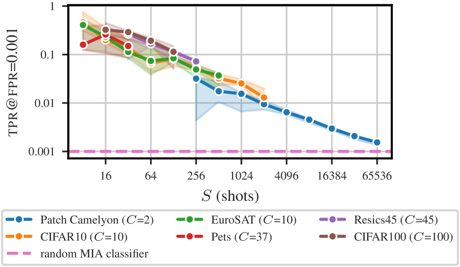
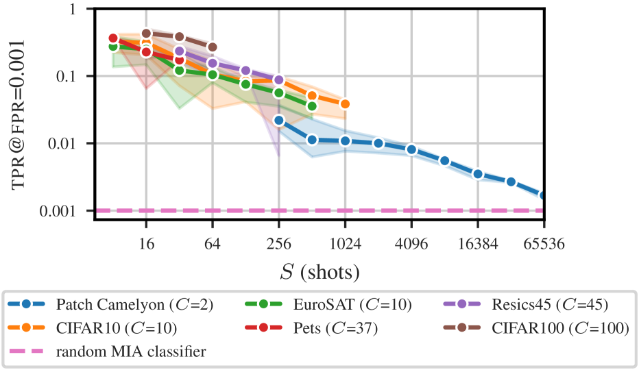
1. Power law: We uncover a power law between the number of examples per class and the vulnerability to MIA (tpr at fixed low fpr) based on extensive experimental data over many data sets with varying sizes (See Figure 2(a)).

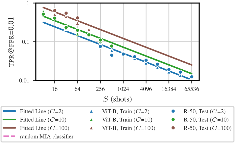
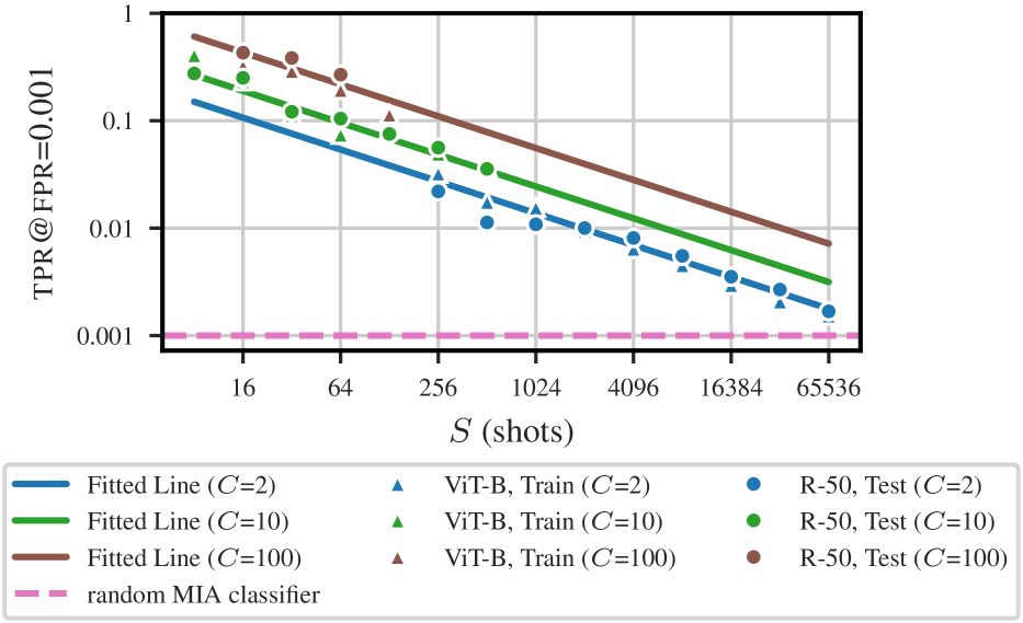
2. Regression model: We utilize the observations to train a regression model to predict MIA vulnerability (tpr at fixed low fpr) based on examples per class ($S$) and number of classes ($C$) and show both very good fit on the training data as well as good prediction quality on unseen data from a different feature extractor (See Figure 3).

Additionally, in Section 6 we extend the analysis to individual samples and discover a correlation between vulnerability of individual samples and the gradient norms during training. We further study the correlation between sample’s vulnerability and the similarity to the other samples in the feature space.

2 Background

Notation for the properties of the training data set $\mathcal{\mathcal{D}}$:

• $C$ for the number of classes

• $S$ for shots (examples per class)

• $\mathcal{|\mathcal{D}|}$ for training data set size ($\mathcal{|\mathcal{D}|}=CS$)

We denote the number of MIA shadow models with $M$.

Membership inference attacks (MIAs) aim to infer whether a particular sample was part of the training set of the targeted model Shokri et al. (2017). Thus, they can be used to determine lower bounds on the privacy leakage of models to complement the theoretical upper bounds obtained through differential privacy.

Likelihood Ratio attack (LiRA; Carlini et al., 2022) While many different MIAs have been proposed Hu et al. (2022), in this work we consider the SOTA: the Likelihood Ratio Attack (LiRA). LiRA assumes an attacker that has black-box access to the attacked model, knows the training data distribution, the training set size, the model architecture, hyperparameters and training algorithm. Based on this information, the attacker can train so-called shadow models (Shokri et al., 2017) which imitate the model under attack but for which the attacker knows the training data set.

LiRA exploits the observation that the value of the loss function used to train a model is often lower for examples that have been part of the training set than for examples that have not been. For a target sample $x$, LiRA trains the shadow models: 1 with $x$ as a part of the training set ($x\in\mathcal{D}$) 2 and without $x$ in the training set ($x\notin\mathcal{D}$) . After training the shadow models, $x$ is passed through the shadow models, and based on the losses (or predictions) two Gaussian distributions are formed, one for the losses of $x\in\mathcal{D}$ shadow models and one for the $x\notin\mathcal{D}$. Finally the attacker computes the loss for the point $x$ using the model under attack and determines using a likelihood ratio test on the distributions built from the shadow models whether it is more likely that $x\in\mathcal{D}$ or $x\notin\mathcal{D}$. Carlini et al. (2022) proposed an optimization for performing LiRA for multiple models and points without training a computationally infeasible amount of shadow models. We utilize this optimization in our experiments.

In Appendix A we provide background on Differential privacy (DP; Dwork et al., 2006b) and DP stochastic gradient descent (DP-SGD) that we use for training DP models.

3 Methods

In this Section, we introduce the preliminaries for evaluating MIA vulnerability.

3.1 Measuring MIA vulnerability

Using the likelihood-ratios from LiRA Carlini et al. (2022) as a score, we can build a binary classifier to predict whether sample belongs to the training data or not. The operational characteristics of such classifier can be used to measure the success of the MIA. More specifically, throughout the rest of the paper, we will use the true positive rate (tpr) at a specific false positive rate (fpr) as a measure for the vulnerability. Identifying even a small number of samples with high confidence is considered harmful (Carlini et al., 2022) and thus we focus on the regions of small fpr.

The tpr and fpr can be also connected to DP. Kairouz et al. (2015) have shown in Equation 1 that any classifier distinguishing the training samples based on the results of a DP algorithm has an upper bound for the tpr that depends on the privacy parameters $(\epsilon,\delta)$. Since MIA is trying to build exactly these types of classifiers, we can use the upper bounds by Kairouz et al. (2015) to validate the privacy claims, and also to better understand the gap between the theoretical privacy guarantees and the realistic attacks.

Theorem 1 (Kairouz et al. (2015)).

A mechanism $\mathcal{M}:\mathcal{X}\to\mathcal{Y}$ is $(\epsilon,\delta)$-DP if and only if for all adjacent $\mathcal{D}\sim\mathcal{D}^{\prime}$

$$\mathrm{TPR}\leq\min\{e^{\epsilon}\mathrm{FPR}+\delta,1-e^{-\epsilon}(1-\delta-\mathrm{FPR})\}\ .$$ (1)

3.2 Measuring the uncertainty for TPR

The tpr values from the LiRA based classifier can be seen as maximum likelihood-estimators for the probability of producing true positives among the positive samples. Since we have a finite number of samples for our estimation, it is important to estimate the uncertainty in these estimator. Therefore, when we report the tpr values for single repeat of the learning algorithm, we estimate the stochasticity of the tpr estimate by using Clopper-Pearson intervals Clopper & Pearson (1934). Given tp true positives among p positives, the $1-\alpha$ confidence Clopper-Pearson interval for the tpr is given as

$$\begin{split}&B(\alpha/2;\textsc{tp},\textsc{p}-\textsc{tp}+1)<\textsc{tpr}\\ &\textsc{tpr}<B(1-\alpha/2;\textsc{tp}+1,\textsc{p}-\textsc{tp}),\end{split}$$ (2)

where $B(q;a,b)$ is the $q$th-quantile of $\text{Beta}(a,b)$ distribution.

4 Experiment overview

Throughout the experiments, we utilize LiRA to understand the vulnerability of the trained models.

We fine-tune pre-trained models on sensitive downstream data sets and assess the vulnerability using LiRA. We use the following setup for all experiments:

• Pre-trained models. BiT-M-R50x1 (R-50; Kolesnikov et al., 2020) with 23.5M parameters and Vision Transformer ViT-Base-16 (ViT-B; Dosovitskiy et al., 2021) with 85.8M parameters, both pre-trained on the ImageNet-21K data set (Russakovsky et al., 2015)

• Parameterization. Due to computational cost we only consider fine-tuning subsets of the model parameters. We consider the following configurations: 1 Head: training a linear last layer classifier on top of the pre-trained model 2 FiLM: Head and additionally training parameter-efficient FiLM (Perez et al., 2018) adapters scattered throughout the network (see Section B.1)

• Fine-tuning data sets. We utilize different fine-tuning data sets (see Section B.3 for details) with different $S$, $C$ and $|\mathcal{D}|$ as specified in the experiments.

• Hyperparameter optimization (HPO). We utilize the library Optuna Akiba et al. (2019) with the Tree-structured Parzen Estimator (TPE; Bergstra et al., 2011) sampler with 20 iterations. We optimize the batch size, learning rate and number of epochs. Additionally for DP-SGD we optimize the clipping norm. Details in Section B.2.

• DP-SGD. We are using Opacus Yousefpour et al. (2021) and compute the noise multiplier based on the target ($\epsilon,\delta$).

• DP Accounting. We use numerical privacy accounting for accurate evaluation of the cumulative privacy loss of the optimisation (Koskela et al., 2020, 2021) using the PRV accountant (Gopi et al., 2021).

• LiRA. We base our experiments on the publically available source code of Carlini et al. (2022). We utilize $M=256$ shadow models unless specified otherwise.

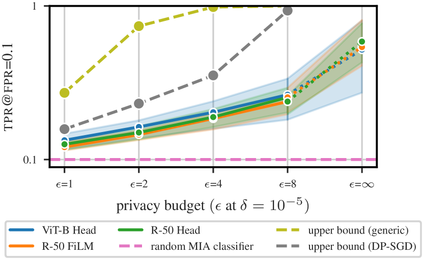
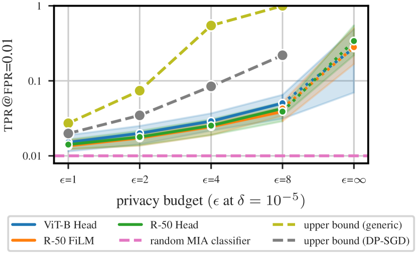
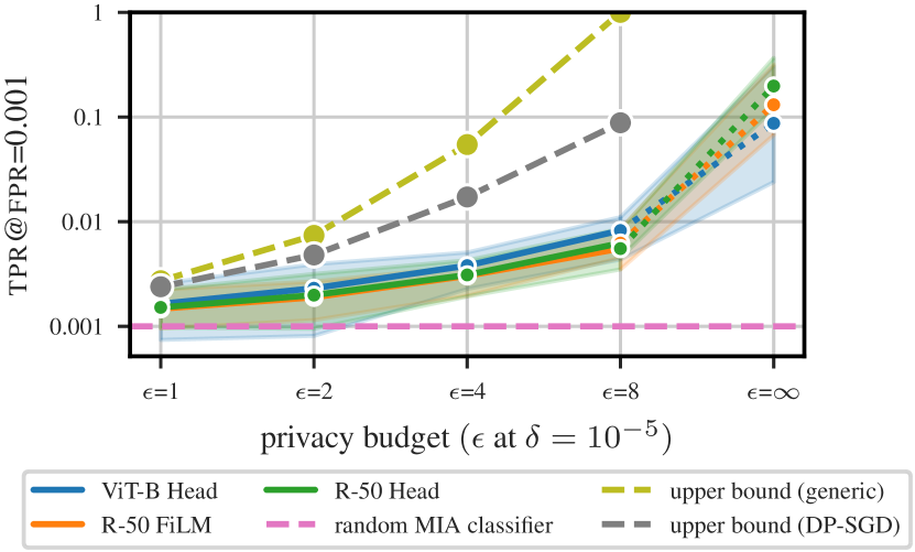
We illustrate the effectiveness of LiRA and the effect of different levels of DP on the MIA vulnerability (tpr at $\textsc{fpr}=0.001$) in Figure 1. It shows the MIA vulnerability as a function of privacy budget (additional versions for different fprs in Figure A.1) and two upper bounds on the tpr at fpr emerging from the theoretical guarantees of DP-SGD.

Figure 1: MIA vulnerability (tpr at $\textsc{fpr}=0.001$) as a function of privacy budget ($\epsilon$ at $\delta=10^{-5}$) when attacking different backbones fine-tuned on CIFAR10 and CIFAR100 at $S\in\{25,50\}$. The solid line displays the median and the error bars the minimum of the lower bounds and the maximum of the upper bounds for the Clopper-Pearson CIs over 15 seeds. The upper bound is the theoretical DP bound based on Kairouz et al. (2015). We present the bound computed with $\delta=10^{-5}$ as well as the optimal bound based on multiple $\delta$.

We compute the upper bounds using the method of Kairouz et al. (2015) in Equation 1. Simply using $\delta=10^{-5}$ and the associated $\epsilon$ gives a relatively weak bound, that can be sharpened considerably by finding an optimal $\delta$ and corresponding $\epsilon(\delta)$, which is made possible by the particular mechanism deployed, that gives the tightest possible bound. For the attacked few-shot models the bounds are quite tight for the medium privacy budget of $\epsilon=1$ but very loose at low privacy budgets of $\epsilon=8$ and thus meaningless for low privacy levels.

5 Predicting MIA vulnerability for data sets

In this Section, we investigate how different properties of data sets affect the MIA vulnerability in the non-DP setting. Based on our observations, we propose a method to predict the vulnerability to MIA using these properties of the data set.

We base our experiments on a subset of the few-shot benchmark VTAB  (Zhai et al., 2019) that achieves a classification accuracy $>80\%$ and thus would considered to be used by practitioners. For more detailed descriptions of the data sets, see Table A2. In this Section, we will focus on a fine-tuned last layer classifier (Head) trained on top of a ViT-B, pre-trained on ImageNet-21k Russakovsky et al. (2015). The results for using R-50 as a backbone can be found in Section C.1.

5.1 Correlations with data set properties

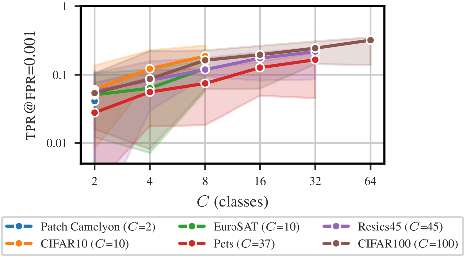
Using the setting described above, we study how the number of classes and the number of shots affect the vulnerability (tpr at fpr as described in Section 3.1). We make the following observations:

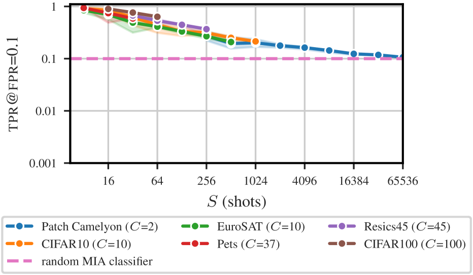
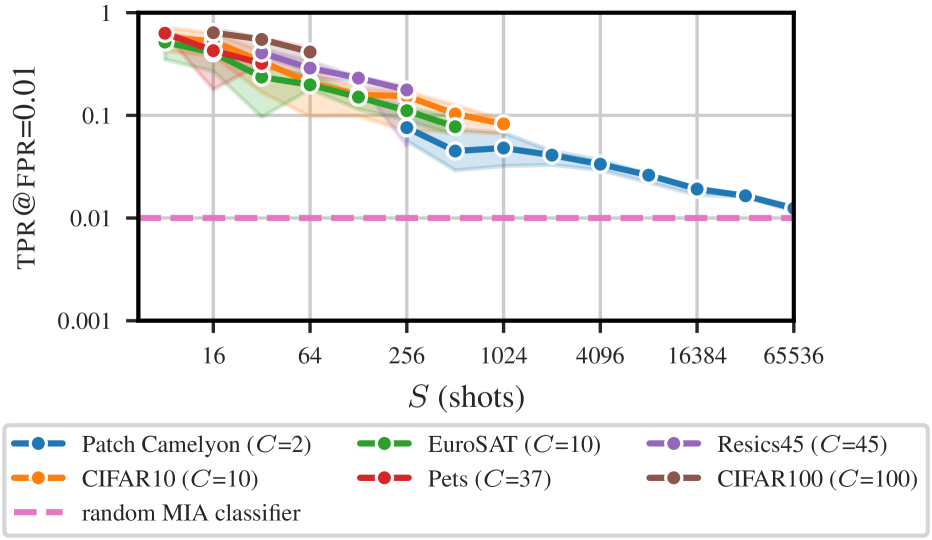
• A larger number of $S$ (shots) decrease the vulnerability in a power law relation as demonstrated in Figure 2(a). We provide further evidence of this in Figures A.2, A3 and A4 in the Appendix.

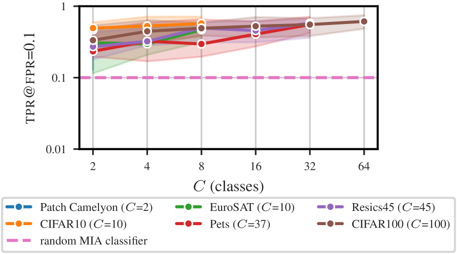
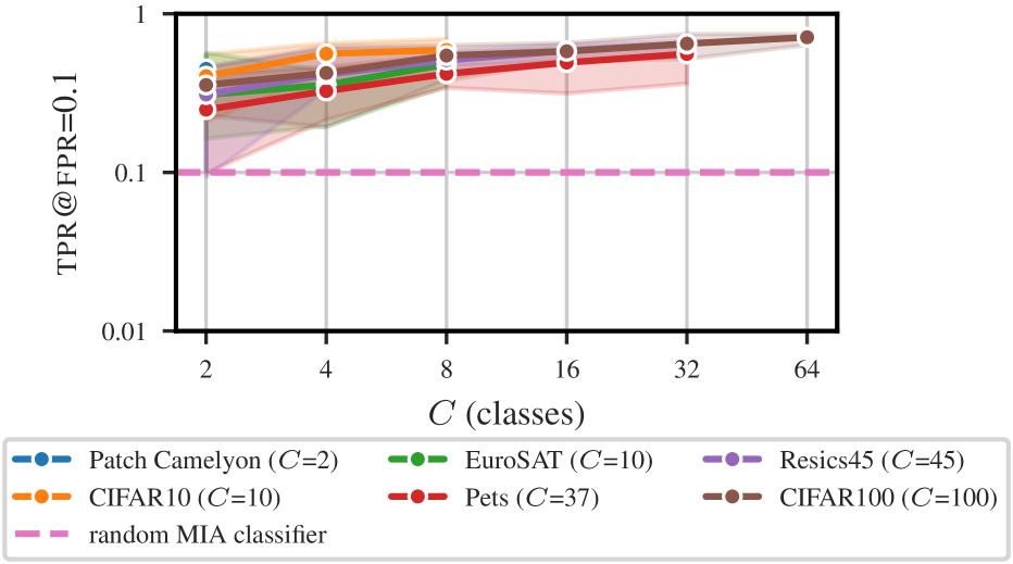
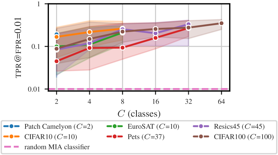
• Contrary, a larger number of $C$ (classes) increases the vulnerability as demonstrated in Figure 2(b) with further evidence in Figures A.3, A5 and A6 in the Appendix. However, the trend w.r.t. $C$ is not as clear as with $S$.

(a) as function of $S$ (shots)

(b) as function of $C$ (classes)

Figure 2: MIA vulnerability (tpr at $\textsc{fpr}=0.001$) as a function of dataset properities when attacking a ViT-B Head fine-tuned without DP on different data sets. The solid line displays the median and the error bars the minimum of the lower bounds and maximum of the upper bounds for the Clopper-Pearson CIs over multiple seeds (6 for Figure 2(a) and 12 for Figure 2(b))

5.2 Model to predict data set vulnerability

Based on the trends seen in Figures 2(b) and 2(a), we fit a linear regression model using the logarithmic transform of $C,S$ to predict the tpr (also logarithmically transformed) with statsmodels Seabold & Perktold (2010). The general form of the model can be found in Equation 3 where $\beta_{S},\beta_{C}$ and $\beta_{0}$ are the learnable regression parameters.

$$\log_{10}(\textsc{tpr})=\beta_{S}\log_{10}(S)+\beta_{C}\log_{10}(C)+\beta_{0}$$ (3)

We utilize MIA results of ViT-B (see Table A3) as the training data and use R-50 (see Table A4) as the test data to investigate if the vulnerability prediction model generalizes to a completely different backbone.

The parameters of the prediction model fitted to the training data (note that the parameters are specific to $\textsc{fpr}=0.001$) are $\beta_{S}=-0.492,\beta_{C}=0.357$ and $\beta_{0}=-0.486$. Based on the $R^{2}$ score ($R^{2}=0.917$), our model fits the data extremely well. Furthermore, Figure 3 shows that the model is robust to a change of feature extractor, as it is able to predict the tpr for R-50 despite being trained on ViT-B (test $R^{2}=0.740$). See Section C.1.3 for further supporting results at $\textsc{fpr}\in\{0.1,0.01\}$.

Figure 3: Predicted MIA vulnerability (tpr at $\textsc{fpr}=0.001$) as a function of $S$ (shots) using a model based on Equation 3 fitted Table A3 (ViT-B). The dots show the median tpr for the train set (ViT-B; Table A3) and the test set (R-50; Table A4) over six seeds (datasets: Patch Camelyon, EuroSAT and CIFAR100).

6 MIA vulnerability for data samples

This Section extends our investigation from the data set level properties studied in Section 5 to individual data sample level properties. Previously Yu et al. (2023) have studied correlations between classes and privacy risk before, but in comparison to their study, we look at data samples independent from classes.

We will focus on a fine-tuned last layer classifier (Head) trained on top of a ViT-B, pre-trained on ImageNet-21k Russakovsky et al. (2015). We investigate two data sample properties that could potentially influence the vulnerability (tpr at fpr) of data points:

• Per-sample gradients: Per-sample gradients form the basis for DP individual accounting Feldman & Zrnic (2021); Koskela et al. (2023). In individual accounting a larger sum of gradient norms results in a higher individual privacy loss. Our hypothesis is that this holds also for MIA vulnerability in non-DP settings.

• Vector space distances: The pre-trained feature extractors project images into a vector space in which one can compute distances between individual data samples. Our hypothesis is that data samples that are further away from other data samples are easier to distinguish.

We study individual samples, but aggregate the results over multiple data samples by binning the samples based on their data sample properties to reduce the noise. For each data sample we compute its property and assign the sample to a bin based on its percentile in relation to other samples. We then compute the tpr at fpr for each bin. We finally report for each data property bin the percentile of the tpr at fpr.

Figure 4: MIA vulnerability (tpr at fpr; percentiles among a seed) as a function of data sample properties (binned among a seed). The results have been obtained over 6 seeds with $S=256$ (Patch Camelyon) and $S=64$ (CIFAR10).

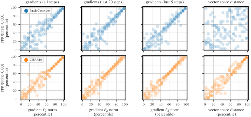
Figure 4 shows the observed relationships between the MIA vulnerability and the average individual gradient norms and the vector space distance. We find that:

• Per-sample gradients: The average gradient norms are correlated with the vulnerability in all our experiments, but the strength of the correlation depends how many steps are taken into account. Generally, we observe that the correlation is stronger when we only consider the gradients at the end of the training (either the last 20 or 5 steps). This is different from the individual accounting methods that rely on the whole gradient trace for DP accounting.

• Vector space distances: The distance of data samples to their nearest neighbor correlates with the vulnerability for CIFAR10, but not for Patch Camelyon. We leave a more comprehensive study of this correlation and its limitations for future work.

7 Discussion

As DP reduces the utility of models, it is important to understand also when it is necessary. Our results on MIA vulnerability as a function of data set properties display a strong power law dependence on the number of examples per class. This leads to an unfortunate dilemma: DP seems most important in the small data regime where it likely reduces the model utility the most.

Limitations

Due to computational constraints, we only report results on transfer learning with fine-tuning only a part of the model.

Appendix A Background

Differential privacy (DP; Dwork et al., 2006b) is the gold standard for formalizing privacy guarantees. $(\epsilon,\delta)$-DP (Dwork et al., 2006a) has a privacy budget consisting of $\epsilon\geq 0$ and $\delta\in[0,1]$, where smaller values correspond to a stronger privacy guarantee. We refer to Dwork & Roth (2014) for a comprehensive intro to DP.

DP deep learning utilizes DP-SGD (Rajkumar & Agarwal, 2012; Song et al., 2013; Abadi et al., 2016), which is the DP adaptation of stochastic gradient descent. DP-SGD clips per-sample gradients to a pre-determined norm to limit the influence of each sample and adds Gaussian noise the sum of the clipped gradients.

Clipping the gradients and adding Gaussian noise in DP-SGD typically comes with a cost in accuracy. This decrease in accuracy can be alleviated through transfer-learning. Publically available pre-trained models are fine-tuned with DP-SGD on sensitive downstream data sets. Both in NLP (Li et al., 2022; Yu et al., 2022) and computer vision (Kurakin et al., 2022; De et al., 2022; Mehta et al., 2022; Cattan et al., 2022; Tobaben et al., 2023) transfer-learning significantly closes the gap between non-private and private training. Tramèr et al. (2022) critically discuss this line of work and the implication of relying on pre-trained models.

Appendix B Training details

B.1 Parameterization

We utilize pre-trained feature extractors BiT-M-R50x1 (R-50) (Kolesnikov et al., 2020) with 23.5M parameters and Vision Transformer ViT-Base-16 (ViT-B) (Dosovitskiy et al., 2021) with 85.8M parameters, both pretrained on the ImageNet-21K data set (Russakovsky et al., 2015). We download the feature extractor checkpoints from the respective repositories.

Following Tobaben et al. (2023) that show the favorable trade-off of parameter-efficient fine-tuning between computational cost, utility and privacy even for small data sets, we only consider fine-tuning subsets of all feature extractor parameters. We consider the following configurations:

• Head: We train a linear layer on top of the pre-trained feature extractor.

• FiLM: In addition to the linear layer from Head, we fine-tune parameter-efficient FiLM (Perez et al., 2018) adapters scattered throughout the network. While a diverse set of adapters has been proposed, we utilize FiLM as it has been shown to be competitive in prior work (Shysheya et al., 2023; Tobaben et al., 2023).

B.2 Hyperparameter tuning

Our hyperparameter tuning is heavily inspired by the comprehensive few-shot experiments by Tobaben et al. (2023). We utilize their hyperparameter tuning protocol as it has been proven to yield SOTA results for (DP) few-shot models.

Given the input $\mathcal{\mathcal{D}}$ data set we perform hyperparameter tuning by splitting the $\mathcal{\mathcal{D}}$ into 70$\%$ train and 30$\%$ validation. We then perform the specified iterations of hyperparameter tuning using the tree-structured Parzen estimator (Bergstra et al., 2011) strategy as implemented in Optuna (Akiba et al., 2019) to derive a set of hyperparameters that yield the highest accuracy on the validation split. This set of hyperparameters is subsequently used to train all shadow models. Details on the set of hyperparameters that are tuned and their ranges can be found in Table A1. For DP training, we compute the required noise multiplier depending on the target $(\epsilon,\delta)$-DP privacy budget.

Table A1: Hyperparameter ranges used for the Bayesian optimization with Optuna.

	lower bound	upper bound
batch size	10	$|\mathcal{D}|$
clipping norm	0.2	10
epochs	1	200
learning rate	1e-7	1e-2
noise multiplier	Based on target $\epsilon$

B.3 Datasets

Table A2 shows the used data sets in the paper. We base our experiments on a subset of the the few-shot benchmark VTAB (Zhai et al., 2019) that achieves a classification accuracy $>80\%$ and thus would considered to be used by a practitioner. Additionally, we add CIFAR10 that is not part of the original VTAB benchmark.

Table A2: Used datasets in the paper, their minimum and maximum shots $S$ and maximum number of classes $C$ and their test accuracy when fine-tuning a non-DP ViT-B Head. The test accuracy for EuroSAT and Resics45 is computed on the part of the training split that is not used for training the particular model due to both datasets missing an official test split. Note that LiRA requires $2S$ for training the shadow models and thus $S$ is smaller than when only performing fine-tuning.

dataset	(max.)	min.	max.	test accuracy	test accuracy
	$C$	$S$	$S$	(min. $S$)	(max. $S$)
Patch Camelyon (Veeling et al., 2018)	2	256	65536	82.8%	85.6%
CIFAR10 (Krizhevsky, 2009)	10	8	2048	92.7%	97.7%
EuroSAT (Helber et al., 2019)	10	8	512	80.2%	96.7%
Pets (Parkhi et al., 2012)	37	8	32	82.3%	90.7%
Resics45 (Cheng et al., 2017)	45	32	256	83.5%	91.6%
CIFAR100 (Krizhevsky, 2009)	100	16	128	82.2%	87.6%

Appendix C Additional results

In this section, we provide tabular results for our experiments and additional figures that did not fit into the main paper.

(a) tpr at $\textsc{fpr}=0.1$

(b) tpr at $\textsc{fpr}=0.01$

(c) tpr at $\textsc{fpr}=0.001$

Figure A.1: MIA vulnerability as a function of privacy budget ($\epsilon$ at $\delta=10^{-5}$) when attacking different backbones fine-tuned on CIFAR10 and CIFAR100 at $S\in\{25,50\}$. The solid line displays the median and the error bars the minimum of the lower bounds and the maximum of the upper bounds for the Clopper-Pearson CIs over 15 seeds. The DP bounds are the theoretical DP bounds based on Kairouz et al. (2015) where the naive DP bound is computed with $\delta=10^{-5}$ and the tight DP bound over an interval of deltas and their respective $\epsilon$.

C.1 Additional results for Section 5

This section contains additional results for Section 5.

C.1.1 Vulnerability as a function of shots

This section displays additional results to Figure 2(a) for fpr $\in\{0.1,0.01,0.001\}$ for ViT-B and R-50 in in Figures A.2, A3 and A4.

(a) ViT-B Head tpr at $\textsc{fpr}=0.1$

(b) R-50 Head tpr at $\textsc{fpr}=0.1$

(c) ViT-B Head tpr at $\textsc{fpr}=0.01$

(d) R-50 Head tpr at $\textsc{fpr}=0.01$

(e) ViT-B Head tpr at $\textsc{fpr}=0.001$

(f) R-50 Head tpr at $\textsc{fpr}=0.001$

Figure A.2: MIA vulnerability as a function of shots (examples per class) when attacking a pre-trained ViT-B and R-50 Head trained without DP on different downstream data sets. The errorbars display the min and max Clopper-Pearson CIs over 6 seeds and the solid line the median.

Table A3: Median MIA vulnerability over six seeds as a function of $S$ (shots) when attacking a Head trained without DP on-top of a ViT-B. The ViT-B is pre-trained on ImageNet-21k.

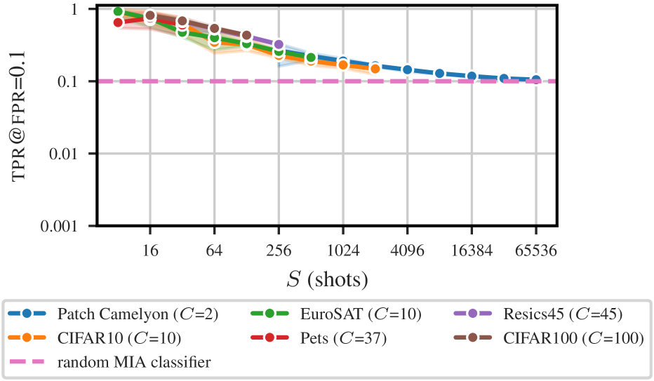
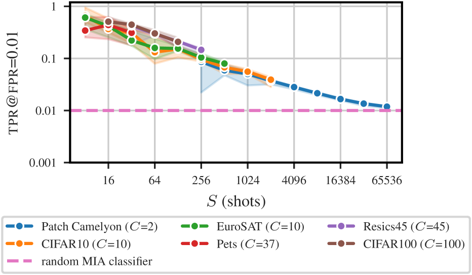
dataset classes ($C$) shots ($S$) tpr@fpr=0.1 tpr@fpr=0.01 tpr@fpr=0.001 Patch Camelyon (Veeling et al., 2018) 2 256 0.266 0.086 0.032 512 0.223 0.059 0.018 1024 0.191 0.050 0.015 2048 0.164 0.037 0.009 4096 0.144 0.028 0.007 8192 0.128 0.021 0.005 16384 0.118 0.017 0.003 32768 0.109 0.014 0.002 65536 0.105 0.012 0.002 CIFAR10 (Krizhevsky, 2009) 10 8 0.910 0.660 0.460 16 0.717 0.367 0.201 32 0.619 0.306 0.137 64 0.345 0.132 0.067 128 0.322 0.151 0.082 256 0.227 0.096 0.054 512 0.190 0.068 0.032 1024 0.168 0.056 0.025 2048 0.148 0.039 0.013 EuroSAT (Helber et al., 2019) 10 8 0.921 0.609 0.408 16 0.738 0.420 0.234 32 0.475 0.222 0.113 64 0.400 0.159 0.074 128 0.331 0.155 0.084 256 0.259 0.104 0.049 512 0.213 0.080 0.037 Pets (Parkhi et al., 2012) 37 8 0.648 0.343 0.160 16 0.745 0.439 0.259 32 0.599 0.311 0.150 Resics45 (Cheng et al., 2017) 45 32 0.672 0.425 0.267 64 0.531 0.295 0.168 128 0.419 0.212 0.115 256 0.323 0.146 0.072 CIFAR100 (Krizhevsky, 2009) 100 16 0.814 0.508 0.324 32 0.683 0.445 0.290 64 0.538 0.302 0.193 128 0.433 0.208 0.114

Table A4: Median MIA vulnerability over six seeds as a function of $S$ (shots) when attacking a Head trained without DP on-top of a R-50. The R-50 is pre-trained on ImageNet-21k.

dataset classes ($C$) shots ($S$) tpr@fpr=0.1 tpr@fpr=0.01 tpr@fpr=0.001 Patch Camelyon (Veeling et al., 2018) 2 256 0.272 0.076 0.022 512 0.195 0.045 0.011 1024 0.201 0.048 0.011 2048 0.178 0.041 0.010 4096 0.163 0.033 0.008 8192 0.143 0.026 0.006 16384 0.124 0.019 0.004 32768 0.118 0.016 0.003 65536 0.106 0.012 0.002 CIFAR10 (Krizhevsky, 2009) 10 8 0.911 0.574 0.324 16 0.844 0.526 0.312 32 0.617 0.334 0.183 64 0.444 0.208 0.106 128 0.334 0.159 0.084 256 0.313 0.154 0.086 512 0.251 0.103 0.051 1024 0.214 0.082 0.038 EuroSAT (Helber et al., 2019) 10 8 0.846 0.517 0.275 16 0.699 0.408 0.250 32 0.490 0.236 0.121 64 0.410 0.198 0.105 128 0.332 0.151 0.075 256 0.269 0.111 0.056 512 0.208 0.077 0.036 Pets (Parkhi et al., 2012) 37 8 0.937 0.631 0.366 16 0.745 0.427 0.227 32 0.588 0.321 0.173 Resics45 (Cheng et al., 2017) 45 32 0.671 0.405 0.235 64 0.534 0.289 0.155 128 0.445 0.231 0.121 256 0.367 0.177 0.088 CIFAR100 (Krizhevsky, 2009) 100 16 0.897 0.638 0.429 32 0.763 0.549 0.384 64 0.634 0.414 0.269

C.1.2 Vulnerability as a function of the number of classes

This section displays additional results to Figure 2(b) for fpr $\in\{0.1,0.01,0.001\}$ for ViT-B and R-50 in in Figures A.3, A5 and A6.

(a) ViT-B Head tpr at $\textsc{fpr}=0.1$

(b) R-50 Head tpr at $\textsc{fpr}=0.1$

(c) ViT-B Head tpr at $\textsc{fpr}=0.01$

(d) R-50 Head tpr at $\textsc{fpr}=0.01$

(e) ViT-B Head tpr at $\textsc{fpr}=0.001$

(f) R-50 Head tpr at $\textsc{fpr}=0.001$

Figure A.3: MIA vulnerability as a function of $C$ (classes) when attacking a ViT-B and R-50 Head fine-tuned without DP on different data sets where the classes are randomly sub-sampled and $S=32$. The solid line displays the median and the errorbars the min and max clopper-pearson CIs over 12 seeds.

Table A5: Median MIA vulnerability over 12 seeds as a function of $C$ (classes) when attacking a Head trained without DP on-top of a ViT-B. The Vit-B is pre-trained on ImageNet-21k.

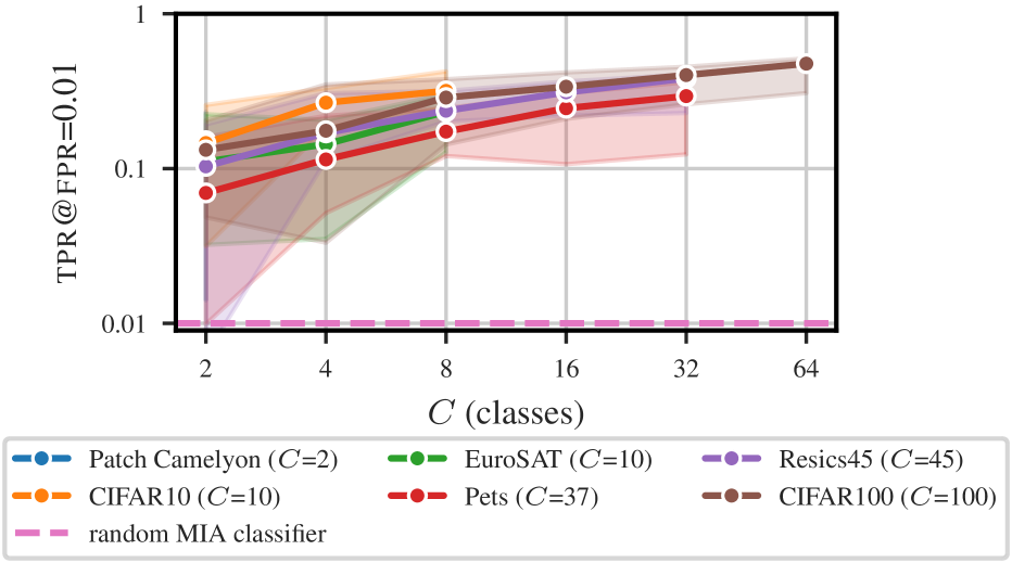
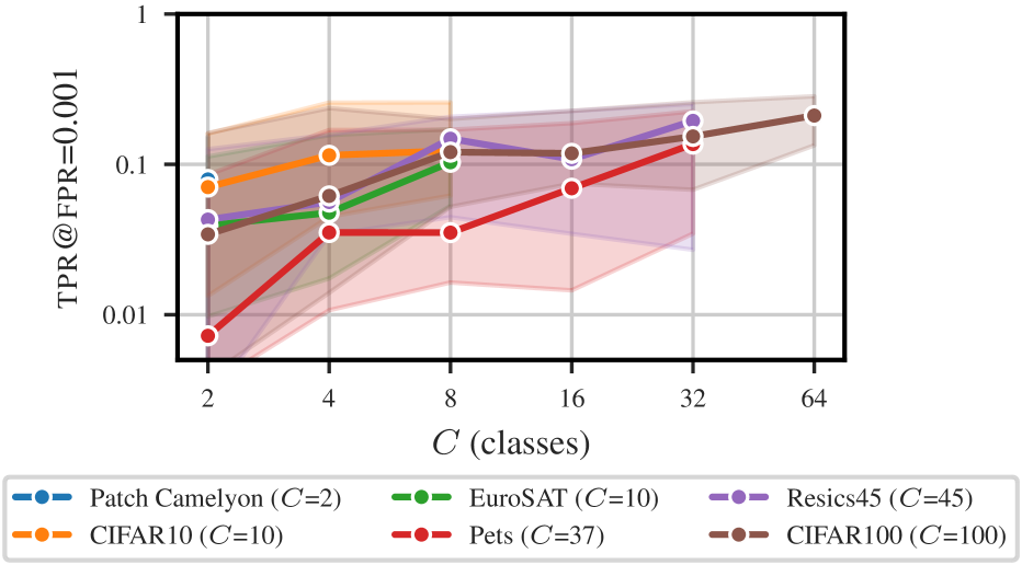
dataset shots ($S$) classes ($C$) tpr@fpr=0.1 tpr@fpr=0.01 tpr@fpr=0.001 Patch Camelyon (Veeling et al., 2018) 32 2 0.467 0.192 0.080 CIFAR10 (Krizhevsky, 2009) 32 2 0.494 0.167 0.071 4 0.527 0.217 0.115 8 0.574 0.262 0.123 EuroSAT (Helber et al., 2019) 32 2 0.306 0.100 0.039 4 0.298 0.111 0.047 8 0.468 0.211 0.103 Pets (Parkhi et al., 2012) 32 2 0.232 0.045 0.007 4 0.324 0.092 0.035 8 0.296 0.094 0.035 16 0.406 0.158 0.069 32 0.553 0.269 0.136 Resics45 (Cheng et al., 2017) 32 2 0.272 0.084 0.043 4 0.322 0.119 0.056 8 0.496 0.253 0.148 16 0.456 0.204 0.108 32 0.580 0.332 0.195 CIFAR100 (Krizhevsky, 2009) 32 2 0.334 0.088 0.035 4 0.445 0.150 0.061 8 0.491 0.223 0.121 16 0.525 0.256 0.118 32 0.553 0.276 0.153 64 0.612 0.350 0.211

Table A6: Median MIA vulnerability over 12 seeds as a function of $C$ (classes) when attacking a Head trained without DP on-top of a R-50. The R-50 is pre-trained on ImageNet-21k.

dataset shots ($S$) classes ($C$) tpr@fpr=0.1 tpr@fpr=0.01 tpr@fpr=0.001 Patch Camelyon (Veeling et al., 2018) 32 2 0.452 0.151 0.041 CIFAR10 (Krizhevsky, 2009) 32 2 0.404 0.146 0.060 4 0.560 0.266 0.123 8 0.591 0.318 0.187 EuroSAT (Helber et al., 2019) 32 2 0.309 0.111 0.050 4 0.356 0.144 0.064 8 0.480 0.233 0.123 Pets (Parkhi et al., 2012) 32 2 0.249 0.068 0.029 4 0.326 0.115 0.056 8 0.419 0.173 0.075 16 0.493 0.245 0.127 32 0.559 0.294 0.166 Resics45 (Cheng et al., 2017) 32 2 0.310 0.103 0.059 4 0.415 0.170 0.083 8 0.510 0.236 0.119 16 0.585 0.311 0.174 32 0.644 0.382 0.218 CIFAR100 (Krizhevsky, 2009) 32 2 0.356 0.132 0.054 4 0.423 0.176 0.087 8 0.545 0.288 0.163 16 0.580 0.338 0.196 32 0.648 0.402 0.244 64 0.711 0.476 0.320

C.1.3 Predicting data set vulnerability as function of $S$ and $C$

Table A7: Results for fitting Equation 3 with statsmodels Seabold & Perktold (2010) to ViT Head data at fpr $\in\{0.1,0.01,0.001\}$. We utilize an ordinary least squares. The test $R^{2}$ assesses the fit to the data of R-50 Head.

coeff. fpr $R^{2}$ test $R^{2}$ coeff. value std. error $t$ $p>|z|$ coeff. $[0.025$ coeff. $0.975]$ $\beta_{S}$ (for $S$) 0.1 0.924 0.898 -0.237 0.008 -30.994 0.000 -0.252 -0.222 0.01 0.937 0.839 -0.380 0.012 -31.818 0.000 -0.403 -0.356 0.001 0.917 0.740 -0.492 0.019 -26.143 0.000 -0.530 -0.455 $\beta_{C}$ (for $C$) 0.1 0.924 0.898 0.095 0.014 6.992 0.000 0.068 0.121 0.01 0.937 0.839 0.226 0.021 10.680 0.000 0.184 0.268 0.001 0.917 0.740 0.357 0.033 10.677 0.000 0.291 0.423 $\beta_{0}$ (intercept) 0.1 0.924 0.898 -0.008 0.029 -0.274 0.785 -0.064 0.049 0.01 0.937 0.839 -0.224 0.045 -5.006 0.000 -0.312 -0.136 0.001 0.917 0.740 -0.486 0.071 -6.879 0.000 -0.626 -0.347

(a) tpr at $\textsc{fpr}=0.1$

(b) tpr at $\textsc{fpr}=0.01$

(c) tpr at $\textsc{fpr}=0.001$

Figure A.4: Predicted MIA vulnerability as a function of $S$ (shots) using a model based on Equation 3 fitted Table A3 (ViT-B). The dots show the median tpr for the train set (ViT-B; Table A3) and the test set (R-50; Table A4) over six seeds. Note that the dots for $C=10$ are for EuroSAT.

References

- Abadi et al. (2016) Martín Abadi, Andy Chu, Ian J. Goodfellow, H. Brendan McMahan, Ilya Mironov, Kunal Talwar, and Li Zhang. Deep learning with differential privacy. In Edgar R. Weippl, Stefan Katzenbeisser, Christopher Kruegel, Andrew C. Myers, and Shai Halevi (eds.), Proceedings of the 2016 ACM SIGSAC Conference on Computer and Communications Security, Vienna, Austria, October 24-28, 2016, pp. 308–318. ACM, 2016. doi: 10.1145/2976749.2978318.
- Akiba et al. (2019) Takuya Akiba, Shotaro Sano, Toshihiko Yanase, Takeru Ohta, and Masanori Koyama. Optuna: A next-generation hyperparameter optimization framework. In Ankur Teredesai, Vipin Kumar, Ying Li, Rómer Rosales, Evimaria Terzi, and George Karypis (eds.), Proceedings of the 25th ACM SIGKDD International Conference on Knowledge Discovery & Data Mining, KDD 2019, Anchorage, AK, USA, August 4-8, 2019, pp. 2623–2631. ACM, 2019. doi: 10.1145/3292500.3330701.
- Balle et al. (2022) Borja Balle, Giovanni Cherubin, and Jamie Hayes. Reconstructing training data with informed adversaries. In 43rd IEEE Symposium on Security and Privacy, SP 2022, San Francisco, CA, USA, May 22-26, 2022, pp. 1138–1156. IEEE, 2022. doi: 10.1109/SP46214.2022.9833677.
- Bergstra et al. (2011) James Bergstra, Rémi Bardenet, Yoshua Bengio, and Balázs Kégl. Algorithms for hyper-parameter optimization. In John Shawe-Taylor, Richard S. Zemel, Peter L. Bartlett, Fernando C. N. Pereira, and Kilian Q. Weinberger (eds.), Advances in Neural Information Processing Systems 24: 25th Annual Conference on Neural Information Processing Systems 2011. Proceedings of a meeting held 12-14 December 2011, Granada, Spain, pp. 2546–2554, 2011.
- Carlini et al. (2022) Nicholas Carlini, Steve Chien, Milad Nasr, Shuang Song, Andreas Terzis, and Florian Tramèr. Membership inference attacks from first principles. In 43rd IEEE Symposium on Security and Privacy, SP 2022, San Francisco, CA, USA, May 22-26, 2022, pp. 1897–1914. IEEE, 2022. doi: 10.1109/SP46214.2022.9833649.
- Cattan et al. (2022) Yannis Cattan, Christopher A. Choquette-Choo, Nicolas Papernot, and Abhradeep Thakurta. Fine-tuning with differential privacy necessitates an additional hyperparameter search. CoRR, abs/2210.02156, 2022. doi: 10.48550/arXiv.2210.02156.
- Chen et al. (2020) Dingfan Chen, Ning Yu, Yang Zhang, and Mario Fritz. GAN-leaks: A taxonomy of membership inference attacks against generative models. In Jay Ligatti, Xinming Ou, Jonathan Katz, and Giovanni Vigna (eds.), CCS ’20: 2020 ACM SIGSAC Conference on Computer and Communications Security, Virtual Event, USA, November 9-13, 2020, pp. 343–362. ACM, 2020. doi: 10.1145/3372297.3417238.
- Cheng et al. (2017) Gong Cheng, Junwei Han, and Xiaoqiang Lu. Remote sensing image scene classification: Benchmark and state of the art. Proceedings of the IEEE, 105(10):1865–1883, 2017.
- Clopper & Pearson (1934) C. J. Clopper and E. S. Pearson. The use of confidence or fiducial limits illustrated in the case of the binomial. Biometrika, 26(4):404–413, December 1934. doi: 10.1093/biomet/26.4.404.
- De et al. (2022) Soham De, Leonard Berrada, Jamie Hayes, Samuel L. Smith, and Borja Balle. Unlocking high-accuracy differentially private image classification through scale. CoRR, abs/2204.13650, 2022. doi: 10.48550/arXiv.2204.13650.
- Dosovitskiy et al. (2021) Alexey Dosovitskiy, Lucas Beyer, Alexander Kolesnikov, Dirk Weissenborn, Xiaohua Zhai, Thomas Unterthiner, Mostafa Dehghani, Matthias Minderer, Georg Heigold, Sylvain Gelly, Jakob Uszkoreit, and Neil Houlsby. An image is worth 16x16 words: Transformers for image recognition at scale. In 9th International Conference on Learning Representations, ICLR 2021, Virtual Event, Austria, May 3-7, 2021. OpenReview.net, 2021.
- Dwork & Roth (2014) Cynthia Dwork and Aaron Roth. The algorithmic foundations of differential privacy. Foundations and Trends® in Theoretical Computer Science, 9(3–4):211–407, 2014. ISSN 1551-305X. doi: 10.1561/0400000042.
- Dwork et al. (2006a) Cynthia Dwork, Krishnaram Kenthapadi, Frank McSherry, Ilya Mironov, and Moni Naor. Our data, ourselves: Privacy via distributed noise generation. In Serge Vaudenay (ed.), Advances in Cryptology - EUROCRYPT 2006, 25th Annual International Conference on the Theory and Applications of Cryptographic Techniques, St. Petersburg, Russia, May 28 - June 1, 2006, Proceedings, volume 4004 of Lecture Notes in Computer Science, pp. 486–503. Springer, 2006a. doi: 10.1007/11761679˙29.
- Dwork et al. (2006b) Cynthia Dwork, Frank McSherry, Kobbi Nissim, and Adam D. Smith. Calibrating noise to sensitivity in private data analysis. In Shai Halevi and Tal Rabin (eds.), Theory of Cryptography, Third Theory of Cryptography Conference, TCC 2006, New York, NY, USA, March 4-7, 2006, Proceedings, volume 3876 of Lecture Notes in Computer Science, pp. 265–284. Springer, 2006b. doi: 10.1007/11681878˙14.
- Feldman & Zrnic (2021) Vitaly Feldman and Tijana Zrnic. Individual privacy accounting via a Rényi filter. In Marc’Aurelio Ranzato, Alina Beygelzimer, Yann N. Dauphin, Percy Liang, and Jennifer Wortman Vaughan (eds.), Advances in Neural Information Processing Systems 34: Annual Conference on Neural Information Processing Systems 2021, NeurIPS 2021, December 6-14, 2021, virtual, pp. 28080–28091, 2021.
- Gopi et al. (2021) Sivakanth Gopi, Yin Tat Lee, and Lukas Wutschitz. Numerical composition of differential privacy. In Marc’Aurelio Ranzato, Alina Beygelzimer, Yann N. Dauphin, Percy Liang, and Jennifer Wortman Vaughan (eds.), Advances in Neural Information Processing Systems 34: Annual Conference on Neural Information Processing Systems 2021, NeurIPS 2021, December 6-14, 2021, virtual, pp. 11631–11642, 2021.
- Helber et al. (2019) Patrick Helber, Benjamin Bischke, Andreas Dengel, and Damian Borth. Eurosat: A novel dataset and deep learning benchmark for land use and land cover classification. IEEE Journal of Selected Topics in Applied Earth Observations and Remote Sensing, 12(7):2217–2226, 2019.
- Hu et al. (2022) Hongsheng Hu, Zoran Salcic, Lichao Sun, Gillian Dobbie, Philip S Yu, and Xuyun Zhang. Membership inference attacks on machine learning: A survey. ACM Computing Surveys (CSUR), 54(11s):1–37, 2022.
- Kairouz et al. (2015) Peter Kairouz, Sewoong Oh, and Pramod Viswanath. The composition theorem for differential privacy. In Francis R. Bach and David M. Blei (eds.), Proceedings of the 32nd International Conference on Machine Learning, ICML 2015, Lille, France, 6-11 July 2015, volume 37 of JMLR Workshop and Conference Proceedings, pp. 1376–1385. JMLR.org, 2015.
- Kolesnikov et al. (2020) Alexander Kolesnikov, Lucas Beyer, Xiaohua Zhai, Joan Puigcerver, Jessica Yung, Sylvain Gelly, and Neil Houlsby. Big transfer (BiT): General visual representation learning. In Andrea Vedaldi, Horst Bischof, Thomas Brox, and Jan-Michael Frahm (eds.), Computer Vision - ECCV 2020 - 16th European Conference, Glasgow, UK, August 23-28, 2020, Proceedings, Part V, volume 12350 of Lecture Notes in Computer Science, pp. 491–507. Springer, 2020. doi: 10.1007/978-3-030-58558-7˙29.
- Koskela et al. (2020) Antti Koskela, Joonas Jälkö, and Antti Honkela. Computing tight differential privacy guarantees using FFT. In The 23rd International Conference on Artificial Intelligence and Statistics, (AISTATS 2020), volume 108 of Proceedings of Machine Learning Research, pp. 2560–2569. PMLR, 2020.
- Koskela et al. (2021) Antti Koskela, Joonas Jälkö, Lukas Prediger, and Antti Honkela. Tight differential privacy for discrete-valued mechanisms and for the subsampled Gaussian mechanism using FFT. In The 24th International Conference on Artificial Intelligence and Statistics, (AISTATS 2021), volume 130 of Proceedings of Machine Learning Research, pp. 3358–3366. PMLR, 2021.
- Koskela et al. (2023) Antti Koskela, Marlon Tobaben, and Antti Honkela. Individual privacy accounting with Gaussian differential privacy. In The Eleventh International Conference on Learning Representations, ICLR 2023, Kigali, Rwanda, May 1-5, 2023. OpenReview.net, 2023.
- Krizhevsky (2009) Alex Krizhevsky. Learning multiple layers of features from tiny images. Master’s thesis, University of Toronto, 2009.
- Kurakin et al. (2022) Alexey Kurakin, Steve Chien, Shuang Song, Roxana Geambasu, Andreas Terzis, and Abhradeep Thakurta. Toward Training at ImageNet Scale with Differential Privacy. ArXiv preprint, abs/2201.12328, 2022.
- Li et al. (2022) Xuechen Li, Florian Tramèr, Percy Liang, and Tatsunori Hashimoto. Large language models can be strong differentially private learners. In The Tenth International Conference on Learning Representations, ICLR 2022, Virtual Event, April 25-29, 2022. OpenReview.net, 2022.
- Mehta et al. (2022) Harsh Mehta, Abhradeep Thakurta, Alexey Kurakin, and Ashok Cutkosky. Large scale transfer learning for differentially private image classification. CoRR, abs/2205.02973, 2022. doi: 10.48550/arXiv.2205.02973.
- Nasr et al. (2023) Milad Nasr, Nicholas Carlini, Jonathan Hayase, Matthew Jagielski, A. Feder Cooper, Daphne Ippolito, Christopher A. Choquette-Choo, Eric Wallace, Florian Tramèr, and Katherine Lee. Scalable extraction of training data from (production) language models. CoRR, abs/2311.17035, 2023. doi: 10.48550/ARXIV.2311.17035.
- Németh et al. (2023) Gergely Dániel Németh, Miguel Angel Lozano, Novi Quadrianto, and Nuria Oliver. Addressing membership inference attack in federated learning with model compression. CoRR, abs/2311.17750, 2023. doi: 10.48550/ARXIV.2311.17750.
- Parkhi et al. (2012) Omkar M. Parkhi, Andrea Vedaldi, Andrew Zisserman, and C. V. Jawahar. Cats and dogs. In 2012 IEEE Conference on Computer Vision and Pattern Recognition, Providence, RI, USA, June 16-21, 2012, pp. 3498–3505. IEEE Computer Society, 2012. doi: 10.1109/CVPR.2012.6248092.
- Perez et al. (2018) Ethan Perez, Florian Strub, Harm de Vries, Vincent Dumoulin, and Aaron C. Courville. Film: Visual reasoning with a general conditioning layer. In Sheila A. McIlraith and Kilian Q. Weinberger (eds.), Proceedings of the Thirty-Second AAAI Conference on Artificial Intelligence, (AAAI-18), the 30th innovative Applications of Artificial Intelligence (IAAI-18), and the 8th AAAI Symposium on Educational Advances in Artificial Intelligence (EAAI-18), New Orleans, Louisiana, USA, February 2-7, 2018, pp. 3942–3951. AAAI Press, 2018.
- Rajkumar & Agarwal (2012) Arun Rajkumar and Shivani Agarwal. A differentially private stochastic gradient descent algorithm for multiparty classification. In Neil D. Lawrence and Mark A. Girolami (eds.), Proceedings of the Fifteenth International Conference on Artificial Intelligence and Statistics, AISTATS 2012, La Palma, Canary Islands, Spain, April 21-23, 2012, volume 22 of JMLR Proceedings, pp. 933–941. JMLR.org, 2012.
- Russakovsky et al. (2015) Olga Russakovsky, Jia Deng, Hao Su, Jonathan Krause, Sanjeev Satheesh, Sean Ma, Zhiheng Huang, Andrej Karpathy, Aditya Khosla, Michael S. Bernstein, Alexander C. Berg, and Li Fei-Fei. ImageNet large scale visual recognition challenge. Int. J. Comput. Vis., 115(3):211–252, 2015. doi: 10.1007/S11263-015-0816-Y.
- Seabold & Perktold (2010) Skipper Seabold and Josef Perktold. statsmodels: Econometric and statistical modeling with python. In 9th Python in Science Conference, 2010.
- Shokri et al. (2017) Reza Shokri, Marco Stronati, Congzheng Song, and Vitaly Shmatikov. Membership inference attacks against machine learning models. In 2017 IEEE Symposium on Security and Privacy, SP 2017, San Jose, CA, USA, May 22-26, 2017, pp. 3–18. IEEE Computer Society, 2017. doi: 10.1109/SP.2017.41.
- Shysheya et al. (2023) Aliaksandra Shysheya, John Bronskill, Massimiliano Patacchiola, Sebastian Nowozin, and Richard E. Turner. FiT: parameter efficient few-shot transfer learning for personalized and federated image classification. In The Eleventh International Conference on Learning Representations, ICLR 2023, Kigali, Rwanda, May 1-5, 2023. OpenReview.net, 2023.
- Song et al. (2013) Shuang Song, Kamalika Chaudhuri, and Anand D. Sarwate. Stochastic gradient descent with differentially private updates. In IEEE Global Conference on Signal and Information Processing, GlobalSIP 2013, Austin, TX, USA, December 3-5, 2013, pp. 245–248. IEEE, 2013. doi: 10.1109/GlobalSIP.2013.6736861.
- Tobaben et al. (2023) Marlon Tobaben, Aliaksandra Shysheya, John Bronskill, Andrew Paverd, Shruti Tople, Santiago Zanella Béguelin, Richard E. Turner, and Antti Honkela. On the efficacy of differentially private few-shot image classification. Transactions on Machine Learning Research, 2023. ISSN 2835-8856.
- Tramèr et al. (2022) Florian Tramèr, Gautam Kamath, and Nicholas Carlini. Considerations for differentially private learning with large-scale public pretraining. CoRR, abs/2212.06470, 2022. doi: 10.48550/arXiv.2212.06470.
- Veeling et al. (2018) Bastiaan S Veeling, Jasper Linmans, Jim Winkens, Taco Cohen, and Max Welling. Rotation equivariant cnns for digital pathology. In International Conference on Medical image computing and computer-assisted intervention, pp. 210–218. Springer, 2018.
- Yousefpour et al. (2021) Ashkan Yousefpour, Igor Shilov, Alexandre Sablayrolles, Davide Testuggine, Karthik Prasad, Mani Malek, John Nguyen, Sayan Gosh, Akash Bharadwaj, Jessica Zhao, Graham Cormode, and Ilya Mironov. Opacus: User-friendly differential privacy library in PyTorch. ArXiv preprint, abs/2109.12298, 2021.
- Yu et al. (2022) Da Yu, Saurabh Naik, Arturs Backurs, Sivakanth Gopi, Huseyin A. Inan, Gautam Kamath, Janardhan Kulkarni, Yin Tat Lee, Andre Manoel, Lukas Wutschitz, Sergey Yekhanin, and Huishuai Zhang. Differentially private fine-tuning of language models. In The Tenth International Conference on Learning Representations, ICLR 2022, Virtual Event, April 25-29, 2022. OpenReview.net, 2022.
- Yu et al. (2023) Da Yu, Gautam Kamath, Janardhan Kulkarni, Tie-Yan Liu, Jian Yin, and Huishuai Zhang. Individual privacy accounting for differentially private stochastic gradient descent. Transactions on Machine Learning Research, 2023. ISSN 2835-8856.
- Zhai et al. (2019) Xiaohua Zhai, Joan Puigcerver, Alexander Kolesnikov, Pierre Ruyssen, Carlos Riquelme, Mario Lucic, Josip Djolonga, Andre Susano Pinto, Maxim Neumann, Alexey Dosovitskiy, et al. A large-scale study of representation learning with the visual task adaptation benchmark. ArXiv preprint, abs/1910.04867, 2019.