On the numerical controllability of the two-dimensional heat, Stokes and Navier-Stokes equations

Abstract

The aim of this work is to present some strategies to solve numerically controllability problems for the two-dimensional heat equation, the Stokes equations and the Navier-Stokes equations with Dirichlet boundary conditions. The main idea is to adapt the Fursikov-Imanuvilov formulation, see [A.V. Fursikov, O.Yu. Imanuvilov: Controllability of Evolutions Equations, Lectures Notes Series, Vol. 34, Seoul National University, 1996]; this approach has been followed recently for the one-dimensional heat equation by the first two authors. More precisely, we minimize over the class of admissible null controls a functional that involves weighted integrals of the state and the control, with weights that blow up near the final time. The associated optimality conditions can be viewed as a differential system in the three variables $x_{1}$, $x_{2}$ and $t$ that is second–order in time and fourth–order in space, completed with appropriate boundary conditions. We present several mixed formulations of the problems and, then, associated mixed finite element Lagrangian approximations that are relatively easy to handle. Finally, we exhibit some numerical experiments.

1 Introduction. The controllability problems

Let $\Omega\subset\mathbb{R}^{2}$ be a bounded domain whose boundary $\Gamma:=\partial\Omega$ is regular enough. Let $\omega\subset\Omega$ be a (possibly small) nonempty open subset and assume that $T>0$. We will use the notation $Q_{\tau}=\Omega\times(0,\tau)$, $\Sigma_{\tau}=\Gamma\times(0,\tau)$, $q_{\tau}=\omega\times(0,\tau)$ and $\mathbf{n}=\mathbf{n}(\mathbf{x})$ will denote the outward unit normal to $\Omega$ at any point $\mathbf{x}\in\Gamma$.

Throughout this paper, $C$ will denote a generic positive constant (usually depending on $\Omega$, $\omega$ and $T$) and the bold letters and symbols will stand for vector-valued functions and spaces; for instance $\mathbf{L}^{2}(\Omega)$ is the Hilbert space of the functions $\mathbf{u}=(u_{1},u_{2})$ with $u_{1},u_{2}\in L^{2}(\Omega)$.

This paper is concerned with the global null controllability of the heat equation

$$\left\{\begin{array}[]{lcl}y_{t}-\Delta y+G(\mathbf{x},t)\,y=v1_{\omega}&\hbox{in}&Q_{T},\\ \vskip 3.0pt plus 1.0pt minus 1.0pt\cr\displaystyle y=0&\hbox{on}&\Sigma_{T},\\ \vskip 3.0pt plus 1.0pt minus 1.0pt\cr\displaystyle y(\cdot,0)=y_{0}&\hbox{in}&\Omega\end{array}\right.$$ (1)

and the Stokes equations

$$\left\{\begin{array}[]{lcl}\mathbf{y}_{t}-\nu\Delta\mathbf{y}+\nabla\pi=\mathbf{v}1_{\omega}&\hbox{in}&Q_{T},\\ \vskip 3.0pt plus 1.0pt minus 1.0pt\cr\displaystyle\nabla\cdot\mathbf{y}=0&\hbox{in}&Q_{T},\\ \vskip 3.0pt plus 1.0pt minus 1.0pt\cr\displaystyle\mathbf{y}=\mathbf{0}&\hbox{on}&\Sigma_{T},\\ \vskip 3.0pt plus 1.0pt minus 1.0pt\cr\displaystyle\mathbf{y}(\cdot,0)=\mathbf{y}_{0}&\hbox{in}&\Omega\end{array}\right.$$ (2)

and the local exact controllability to the trajectories of the Navier-Stokes equations

$$\left\{\begin{array}[]{lcl}\mathbf{y}_{t}-\nu\Delta\mathbf{y}+(\mathbf{y}\cdot\nabla)\mathbf{y}+\nabla\pi=\mathbf{v}1_{\omega}&\hbox{in}&Q_{T},\\ \vskip 3.0pt plus 1.0pt minus 1.0pt\cr\displaystyle\nabla\cdot\mathbf{y}=0&\hbox{in}&Q_{T},\\ \vskip 3.0pt plus 1.0pt minus 1.0pt\cr\displaystyle\mathbf{y}=\mathbf{0}&\hbox{on}&\Sigma_{T},\\ \vskip 3.0pt plus 1.0pt minus 1.0pt\cr\displaystyle\mathbf{y}(\cdot,0)=\mathbf{y}_{0}&\hbox{in}&\Omega.\end{array}\right.$$ (3)

Here, $v=v(\mathbf{x},t)$ and $\mathbf{v}=\mathbf{v}(\mathbf{x},t)$ stand for the controls (they are assumed to act on $\omega$ during the time interval $(0,T)$; the symbol $1_{\omega}$ stands for the characteristic function of $\omega$). Moreover, in (1), we assume that $G\in L^{\infty}(Q_{T})$; in (2) and (3), $\nu>0$.

Let us first consider the system (1). It is well known that, for any $y_{0}\in L^{2}(\Omega)$, $T>0$ and $v\in L^{2}(q_{T})$, there exists exactly one solution $y$ to (1), with

$$y\in C^{0}([0,T];L^{2}(\Omega))\cap L^{2}(0,T;H_{0}^{1}(\Omega)).$$

The null controllability problem for (1) at time $T$ is the following:

For any $y_{0}\in L^{2}(\Omega)$ find a control $v\in L^{2}(q_{T})$ such that the associated solution to (1) satisfies

$$y(\mathbf{x},T)=0\quad\hbox{in}\quad\Omega.$$ (4)

The following result is also well known; for a proof, see [13]:

Theorem 1.

The heat equation (1) is null-controllable at any time $T>0$.

Let us now consider the systems (2) and (3). Let us recall the definitions of some usual spaces in the context of incompressible fluids:

$$\mathbf{H}:=\left\{\bm{\varphi}\in\mathbf{L}^{2}(\Omega):\nabla\cdot\bm{\varphi}=0\hbox{ in }\Omega,\leavevmode\nobreak\ \bm{\varphi}\cdot\mathbf{n}=0\hbox{ on }\Gamma\right\},$$

$$\mathbf{V}:=\left\{\bm{\varphi}\in\mathbf{H}^{1}_{0}(\Omega):\nabla\cdot\bm{\varphi}=0\hbox{ in }\Omega\right\},$$

$$U:=\left\{\psi\in H^{1}(\Omega):\int_{\Omega}\psi(\mathbf{x})\,d\mathbf{x}=0\right\}.$$

For any $\mathbf{y}_{0}\in\mathbf{H},\leavevmode\nobreak\ T>0$ and $\mathbf{v}\in\mathbf{L}^{2}(q_{T})$, there exists exactly one solution $(\mathbf{y},\pi)$ to the Stokes equations (2) and (since we are in the $2D$ case), also one solution $(\mathbf{y},\pi)$ to the Navier-Stokes equations (3). In both cases

$$\mathbf{y}\in C^{0}\left([0,T];\mathbf{H}\right)\cap L^{2}\left(0,T;\mathbf{V}\right),\leavevmode\nobreak\ \pi\in L^{2}_{\rm loc}(0,T;U).$$

In the context of the Stokes system (2), the null controllability problem at time $T$ is the following:

For any $\mathbf{y}_{0}\in\mathbf{H}$ find a control $\mathbf{v}\in\mathbf{L}^{2}(q_{T})$ such that the associated solution to (2) satisfies

$$\mathbf{y}(\mathbf{x},T)=\mathbf{0}\quad\hbox{in}\quad\Omega.$$ (5)

Again, the following result is well known; for a proof, see [13]:

Theorem 2.

The Stokes system (2) is null-controllable at any time $T>0$.

Let us recall the concept of exact controllability to the trajectories. The idea is that, even if we cannot reach every element of the state space exactly, we can try to reach (in finite time $T$) any state on any trajectory.

Thus, let $(\overline{\mathbf{y}},\overline{\pi})$ be a solution to the uncontrolled Navier-Stokes equations:

$$\left\{\begin{array}[]{lcl}\overline{\mathbf{y}}_{t}-\nu\Delta\overline{\mathbf{y}}+(\overline{\mathbf{y}}\cdot\nabla)\overline{\mathbf{y}}+\nabla\overline{\pi}=\mathbf{0}&\hbox{in}&Q_{T},\\ \vskip 3.0pt plus 1.0pt minus 1.0pt\cr\displaystyle\nabla\cdot\overline{\mathbf{y}}=0&\hbox{in}&Q_{T},\\ \vskip 3.0pt plus 1.0pt minus 1.0pt\cr\displaystyle\overline{\mathbf{y}}=\mathbf{0}&\hbox{on}&\Sigma_{T},\\ \vskip 3.0pt plus 1.0pt minus 1.0pt\cr\displaystyle\overline{\mathbf{y}}(\cdot,0)=\overline{\mathbf{y}}_{0}&\hbox{in}&\Omega.\end{array}\right.$$ (6)

We will search for controls $\mathbf{v}\in\mathbf{L}^{2}(q_{T})$ such that the associated solutions to (3) satisfy

$$\mathbf{y}(\mathbf{x},T)=\overline{\mathbf{y}}(\mathbf{x},T)\quad\hbox{in}\quad\Omega.$$ (7)

The problem of exact controllability to the trajectories for (3) is the following:

For any $\mathbf{y}_{0}\in\mathbf{H}$ and any trajectory $(\overline{\mathbf{y}},\overline{\pi})$, find a control $\mathbf{v}\in\mathbf{L}^{2}(q_{T})$ such that the associated solution to (3) satisfies (7).

The following result shows that this problem can be solved at least locally when $\overline{\mathbf{y}}$ is bounded; for a proof, see [9, 18]:

Theorem 3.

The Navier-Stokes equations (3) are locally exact controllable to the trajectories $(\overline{\mathbf{y}},\overline{\pi})$ with

$$\overline{\mathbf{y}}\in\mathbf{L}^{\infty}(Q_{T}),\leavevmode\nobreak\ \overline{\mathbf{y}}(\cdot,0)\in\mathbf{V}.$$ (8)

In other words, for any $T>0$ and any solution to $\eqref{TRAJEC}$ satisfying (8), there exists $\varepsilon>0$ with the following property: if $\mathbf{y}_{0}\in\mathbf{V}$ and $\|\mathbf{y}_{0}-\overline{\mathbf{y}}(\cdot,0)\|_{\mathbf{V}}\leq\varepsilon$, one can find controls $\mathbf{v}\in\mathbf{L}^{2}(q_{T})$ such that the associated solutions to (3) satisfy (7).

The aim of this paper is to present efficient strategies for the numerical solution of the previous controllability problems. These problems concern the computation of external heat sources or force fields that can be applied in a small part of the working domain and control the whole system at a prescribed positive time. There are lots of particular situations where this is highly desired; in particular, for theoretical and numerical information on control problems for fluid flows, see [14, 16].

However, the numerical resolution of control problems as those above is not easy. This is due to several reasons:

• In the case of the “linear” problems (1)–(4) and (2)–(5), due to the regularizing effect of the PDEs, the equalities (4) and (5) can be satisfied only in a very small space and standard numerical approximations of the PDEs are unable to capture this. For instance, if we look for a minimal $L^{2}$ norm null control for (1), we are led by duality to an unconstrained extremal problem in a huge space that cannot be approximated efficiently with usual finite dimensional spaces; see however [2, 1] for detailed comments on this issue.

• On the other hand, in (3)–(7) we find the Navier-Stokes system and, obviously, this adds major difficulties. Note that, at present, it is unknown whether or not the exact controllability to the trajectories of (3) holds without smallness assumptions even when $\overline{\mathbf{y}}\equiv\mathbf{0}$.

Remark 1.

In this paper, we will only deal with distributed controls. In fact, in the case of the Stokes and Navier-Stokes equations, it would be more appropriate from the viewpoint of applications to consider boundary controls acting on a part of $\Sigma$; this will be the subject of a forthcoming paper. Note however that, in general terms, a boundary control problem can be re-formulated in the form (2) or (3) by modifying slightly the domain, choosing $\omega$ appropriately (outside the original $\Omega$) and then considering the restriction of the controlled state to the original $\Omega$. $\Box$

The paper is organized as follows.

In Section 2, we deal with the numerical null controllability of the heat equation. Following ideas from [13], we reduce the task to the solution of a boundary-value problem that is fourth-order in space and second-order in time. We present a mixed approximate formulation where we avoid the use of $C^{1}$ finite elements.

In Sections 3 and 4, we present similar numerical strategies to solve numerically the controllability problems considered above for the Stokes and the Navier-Stokes equations. The methods are illustrated with several numerical experiments.

Finally, Section 5 contains several additional comments.

2 A strategy for the computation of null controls for the heat equation

In this Section, we will start from a formulation of the null controllability problem for (1) introduced and extensively used by Fursikov and Imanuvilov, see [13]. We will present some numerical methods essentially obtained by finite dimensional reduction.

Note that this is not the unique efficient approach. The first contribution to the numerical solution of null controllability problems of this kind was due to Carthel, Glowinski and Lions in [4], using duality arguments. However, the resulting problems involve some dual spaces which are very difficult (if not impossible) to approximate numerically. In [20], in the context of approximate controllability, a relaxed observability inequality was given for general semi-discrete (in space) schemes, with the parameter $\varepsilon$ of the order of $\Delta x$. The work [2] extends the results in [20] to the fully discrete situation and proves the convergence towards a semi-discrete control, as the time step $\Delta t$ tends to zero; let us also mention [8], where the authors prove that any controllable parabolic equation, be it discrete or continuous in space, is null-controllable after time discretization through the application of an appropriate filtering of the high frequencies. For a comparison of the results furnished by various methods, see the numerical experiments in [11, 12, 21].

Let us fix the notation

$$Ly:=y_{t}-\Delta y+G(x,t)y,\quad L^{*}p:=-p_{t}-\Delta p+G(x,t)p$$

and let the weights $\rho$, $\chi$ and $\rho_{i}$ be given by

$$\rho(\mathbf{x},t):=e^{\chi(\mathbf{x})/(T-t)},\quad\chi(\mathbf{x}):=K_{1}\left(e^{K_{2}}-e^{\chi_{0}(\mathbf{x})}\right),\quad\rho_{i}(\mathbf{x},t):=(T-t)^{3/2-i}\rho(\mathbf{x},t),\quad i=0,1,2,$$ (9)

where $K_{1}$ and $K_{2}$ are sufficiently large positive constants (depending on $T$) and $\chi_{0}=\chi_{0}(\mathbf{x})$ is a regular bounded function that is positive in $\Omega$, vanishes on $\Gamma$ and satisfies

$$|\nabla\chi_{0}|>0\hbox{ in }\overline{\Omega}\setminus\omega;$$

for a justification of the existence of $\chi_{0}$, see [13].

The main idea relies on considering the extremal problem

$$\left\{\begin{array}[]{llr}\displaystyle\hbox{Minimize }\ J(y,v)={1\over 2}\left(\iint_{Q_{T}}\rho^{2}|y|^{2}\,d\mathbf{x}\,dt+\iint_{q_{T}}\rho_{0}^{2}|v|^{2}\,d\mathbf{x}\,dt\right)\\ \vskip 3.0pt plus 1.0pt minus 1.0pt\cr\displaystyle\hbox{Subject to }\ (y,v)\in\mathcal{H}(y_{0},T).\\ \end{array}\right.$$ (10)

Here, for any $y_{0}\in L^{2}(\Omega)$ and any $T>0$, the linear manifold $\displaystyle\mathcal{H}(y_{0},T)$ is given by

$$\mathcal{H}(y_{0},T):=\{(y,v):v\in L^{2}(q_{T}),\leavevmode\nobreak\ (y,v)\hbox{ satisfies \eqref{heat} and \eqref{null_condition}}\}.$$

We have the following result:

Theorem 4.

For any $y_{0}\in L^{2}(\Omega)$ and any $T>0$, there exists exactly one solution to (10).

This result is a consequence of an appropriate Carleman inequality for the heat equation.

More precisely, let us introduce the space

$$P_{0}:=\{p\in C^{2}(\overline{Q}_{T}):p=0\ \hbox{on}\ \Sigma_{T}\}.$$ (11)

Then, one has:

Proposition 1.

There exists $C_{0}$, only depending on $\Omega$, $\omega$ and $T$, such that the following holds for all $p\in P_{0}$:

$$\begin{array}[]{c}\displaystyle\iint_{Q_{T}}\left[\rho_{2}^{-2}(|p_{t}|^{2}+|\Delta p|^{2})+\rho_{1}^{-2}|\nabla p|^{2}+\rho_{0}^{-2}|p|^{2}\right]d\mathbf{x}\,dt\leq C_{0}\iint_{Q_{T}}(\rho^{-2}|L^{*}p|^{2}+\rho_{0}^{-2}|p|^{2}1_{\omega})\,d\mathbf{x}\,dt.\end{array}$$ (12)

Let us introduce the bilinear form $k(\cdot,\cdot)$, with

$$k(p,p^{\prime}):=\iint_{Q_{T}}\!\left(\rho^{-2}L^{*}p\,L^{*}p^{\prime}+1_{\omega}\rho_{0}^{-2}p\,p^{\prime}\right)d\mathbf{x}\,dt\quad\forall p,p^{\prime}\in P_{0}.$$ (13)

In view of the unique continuation property of the heat equation, $k(\cdot\,,\cdot)$ is a scalar product in $P_{0}$. Indeed, if $p\in P_{0}$, $L^{*}p=0$ in $Q_{T}$, $p=0$ on $\Sigma_{T}$ and $p=0$ in $q_{T}$, then we necessarily have $p\equiv 0$.

Let $P$ be the completion of $P_{0}$ with respect to this scalar product. Then $P$ is a Hilbert space, the functions $p\in P$ satisfy

$$\iint_{Q_{T}}\rho^{-2}|L^{*}p|^{2}\,d\mathbf{x}\,dt+\iint_{q_{T}}\rho_{0}^{-2}|p|^{2}\,d\mathbf{x}\,dt<+\infty$$ (14)

and, from Proposition 1 and a standard density argument, we also have (12) for all $p\in P$.

Another consequence of Proposition 1 is that we can characterize the space $P$ as follows:

$$P=\left\{\,p:p,p_{t},\partial_{j}p,\partial_{jk}p\in L^{2}(0,T-\delta;L^{2}(\Omega))\ \forall\delta>0,\ \eqref{finite-rhs_h}\ \hbox{holds},\ p=0\ \hbox{on}\ \Sigma\,\right\}.$$ (15)

In particular, we see that any $p\in P$ satisfies $p\in C^{0}([0,T-\delta];H_{0}^{1}(\Omega))$ for all $\delta>0$ and, moreover,

$$\|p(\cdot\,,0)\|_{H^{1}_{0}}\leq C\,k(p,p)^{1/2}\quad\forall p\in P.$$ (16)

The main ideas used in this paper to solve numerically (10) rely on the following result :

Theorem 5.

Let the weights $\rho$ and $\rho_{0}$ be chosen as in Proposition 1. Let $(y,v)$ be the unique solution to (10). Then one has

$$y=\rho^{-2}L^{*}p,\quad v=-\rho_{0}^{-2}\bigl{.}p\bigr{|}_{q_{T}},$$ (17)

where $p$ is the unique solution to the following variational equality in the Hilbert space $P$:

$$\left\{\begin{array}[]{l}\displaystyle\iint_{Q_{T}}\left(\rho^{-2}L^{*}p\,L^{*}p^{\prime}+1_{\omega}\rho_{0}^{-2}p\,p^{\prime}\right)\,d\mathbf{x}\,dt=\int_{\Omega}\!y_{0}(\mathbf{x})\,p^{\prime}(\mathbf{x},0)\,d\mathbf{x}\\ \vskip 3.0pt plus 1.0pt minus 1.0pt\cr\displaystyle\forall\leavevmode\nobreak\ p^{\prime}\in P;\ p\in P.\end{array}\right.$$ (18)

We can interpret (18) as the weak formulation of a boundary-value problem for a PDE that is fourth-order in $\mathbf{x}$ and second-order in $t$. Indeed, taking “test functions” $p^{\prime}\in P$ first with $p^{\prime}\in C_{0}^{\infty}(Q_{T})$, then $p^{\prime}\in C^{2}(\overline{\Omega}\times(0,T))$ and finally $p^{\prime}\in C^{2}(\overline{Q}_{T})$, we see easily that $p$ must necessarily satisfy :

$$\left\{\begin{array}[]{lcl}L(\rho^{-2}L^{*}p)+1_{\omega}\rho_{0}^{-2}p=0&\text{in}&Q_{T},\\ \vskip 3.0pt plus 1.0pt minus 1.0pt\cr p=0,\ \ \rho^{-2}L^{*}p=0&\text{on}&\Sigma_{T},\\ \vskip 3.0pt plus 1.0pt minus 1.0pt\cr\bigl{.}\rho^{-2}L^{*}p\bigr{|}_{t=0}=y_{0},\ \ \bigl{.}\rho^{-2}L^{*}p\bigr{|}_{t=T}=0&\text{in}&\Omega.\end{array}\right.$$ (19)

By introducing the linear form $\ell_{0}$, with

$$\langle\ell_{0},p\rangle:=\int_{\Omega}y_{0}(\mathbf{x})\,p(\mathbf{x},0)\,d\mathbf{x}\quad\forall p\in P,$$ (20)

we see from (16) that $\ell_{0}$ is continuous and (18) can be rewritten in the form

$$k(p,p^{\prime})=\langle\ell_{0},p^{\prime}\rangle\quad\forall p^{\prime}\in P;\ p\in P.$$ (21)

Let $P_{h}$ denote a finite dimensional subspace of $P$. A natural approximation of (21) is the following:

$$k(p_{h},p^{\prime}_{h})=\langle\ell_{0},p^{\prime}_{h}\rangle\quad\forall p^{\prime}_{h}\in P_{h};\ p_{h}\in P_{h}.$$ (22)

Thus, to solve numerically the variational equality (21), it suffices to construct explicitly finite dimensional spaces $P_{h}\subset P$. Notice however that this is possible but needs some work. The reason is that, if $p\in P_{h}$, then $\rho^{-1}L^{*}p=\rho^{-1}(-p_{t}-\Delta p+G(\mathbf{x},t)\,p)$ and $\rho_{0}^{-1}p1_{\omega}$ must belong to $L^{2}(Q_{T})$. Consequently, $p_{h}$ must possess first-order time derivatives and up to second-order spatial derivatives in $L_{\rm loc}^{2}(Q_{T})$. Therefore, an approximation based on a standard triangulation of $Q_{T}$ requires spaces $P_{h}$ of functions that must be $C^{0}$ in $(\mathbf{x},t)$ and $C^{1}$ in $\mathbf{x}$ and this can be complex and too expensive. Spaces of this kind are constructed for instance in [5]. For example, good behavior is observed for the so called reduced HTC, Bell or Bogner-Fox-Schmidt finite elements; the reader is referred to [11, 21] for numerical approximations of this kind in the framework of one spatial dimension.

In spite of its complexity, the direct approximation of (22) has an advantage: it is possible to adapt the standard finite element theory to this framework and deduce strong convergence results for the numerical controls and states.

2.1 First mixed formulation with modified variables

Let us introduce the new variable

$$z:=L^{*}p$$ (23)

and let us set $Z:=L^{2}(\rho^{-1};Q_{T})$. Then $z\in Z$ and $L^{*}p-z=0$ (an equality in $Z$).

Notice that this identity can also be written in the form

$$\iint_{Q_{T}}\left(z-L^{*}p\right)\psi\,\,d\mathbf{x}\,dt=0\quad\forall\psi\in C_{0}^{\infty}(Q_{T});$$

Accordingly, we introduce the following reformulation of (21):

$$\left\{\begin{array}[]{l}\displaystyle\iint_{Q_{T}}\left(\rho^{-2}z\,z^{\prime}+\rho_{0}^{-2}p\,p^{\prime}1_{\omega}\right)d\mathbf{x}\,dt+\iint_{Q_{T}}\left(z^{\prime}-L^{*}p^{\prime}\right)\lambda\,\,d\mathbf{x}\,dt=\int_{\Omega}y_{0}(\mathbf{x})\,p^{\prime}(\mathbf{x},0)\,d\mathbf{x},\\ \vskip 3.0pt plus 1.0pt minus 1.0pt\cr\displaystyle\displaystyle\iint_{Q_{T}}\left(z-L^{*}p\right)\lambda^{\prime}\,d\mathbf{x}\,dt=0,\\ \vskip 3.0pt plus 1.0pt minus 1.0pt\cr\displaystyle\displaystyle\qquad\forall(z^{\prime},p^{\prime},\lambda^{\prime})\in Z\times P\times\Lambda;\ ((z,p),\lambda)\in Z\times P\times\Lambda,\end{array}\right.$$ (24)

where, $\Lambda:=L^{2}(\rho;Q_{T})$.

Notice that $Z$, $P$ and $\Lambda$ are the appropriate spaces to keep all the terms in (24) meaningful.

Let us introduce the bilinear forms $\alpha(\cdot\,,\cdot)$ and $\beta(\cdot\,,\cdot)$, with

$$\alpha((z,p),(z^{\prime},p^{\prime})):=\iint_{Q_{T}}\left(\rho^{-2}z\,z^{\prime}+\rho_{0}^{-2}p\,p^{\prime}1_{\omega}\right)\,d\mathbf{x}\,dt\quad\forall(z,p),(z^{\prime},p^{\prime})\in Z\times P$$

and

$$\beta((z,p),\lambda):=\iint_{Q_{T}}\left[L^{*}p-z\right]\lambda\,d\mathbf{x}\,dt\forall(z,p)\in Z\times P,\,\leavevmode\nobreak\ \forall\lambda\in\Lambda$$

and the linear form $\ell:X\mapsto\mathbb{R}$, with

$$\langle\ell,(z,p)\rangle:=\int_{\Omega}\!y_{0}(\mathbf{x})\,p(\mathbf{x},0)\,d\mathbf{x}\,\leavevmode\nobreak\ \forall(z,p)\in Z\times P.$$

Then, $\alpha(\cdot\,,\cdot)$, $\beta(\cdot\,,\cdot)$ and $\ell$ are well-defined and continuous and (24) reads:

$$\left\{\begin{array}[]{l}\displaystyle\alpha((z,q),(z^{\prime},p^{\prime}))+\beta((z^{\prime},p^{\prime}),\lambda)=\langle\ell,(z^{\prime},p^{\prime})\rangle,\\ \vskip 3.0pt plus 1.0pt minus 1.0pt\cr\displaystyle\displaystyle\beta((z,p),\lambda^{\prime})=0,\\ \vskip 3.0pt plus 1.0pt minus 1.0pt\cr\displaystyle\displaystyle\qquad\forall(z^{\prime},p^{\prime},\lambda^{\prime})\in Z\times P\times\Lambda;\ ((z,p),\lambda)\in Z\times P\times\Lambda.\end{array}\right.$$ (25)

This is a mixed formulation of the variational problem (10). In fact, the following result holds:

Proposition 2.

There exists exactly one solution to (25). Furthermore, (21) and (25) are equivalent problems in the following sense:

1. If $((z,p),\lambda)$ solves (25), then $p$ solves (21).

2. Conversely, if $p$ solves (21), there exists $\lambda\in\Lambda$ such that the triplet $((z,p),\lambda)$, with $z:=L^{*}p$ solves (25).

Proof.

Let us introduce the space

$$V:=\{(z,p)\in Z\times P:\beta((z,p),\lambda)=0,\leavevmode\nobreak\ \forall\lambda\in\Lambda\}.$$

We will check that

• $\alpha(\cdot\,,\cdot)$ is coercive in $V$.

• $\beta(\cdot\,,\cdot)$ satisfies the usual “inf-sup” condition with respect to $Z\times P$ and $\Lambda$.

This will be sufficient to guarantee the existence and uniqueness of a solution to (25); see for instance [3, 24].

The proofs of the previous assertions are straightforward. Indeed, we first notice that, for any $(z,p)\in V$, $z=L^{*}p$ and thus

$$\begin{array}[]{lll}\displaystyle\alpha((z,p),(z,p))&=&\displaystyle\iint_{Q_{T}}\left(\rho^{-2}|z|^{2}+\rho_{0}^{-2}|p|^{2}1_{\omega}\ \right)\,d\mathbf{x}\,dt\\ \vskip 3.0pt plus 1.0pt minus 1.0pt\cr\displaystyle&=&\displaystyle{1\over 2}\iint_{Q_{T}}\rho^{-2}|z|^{2}\,d\mathbf{x}\,dt+\frac{1}{2}\iint_{Q_{T}}\rho^{-2}|L^{*}p|^{2}\,d\mathbf{x}\,dt+\iint_{Q_{T}}\rho_{0}^{-2}|p|^{2}1_{\omega}\,d\mathbf{x}\,dt\\ \vskip 3.0pt plus 1.0pt minus 1.0pt\cr\displaystyle&=&\displaystyle\frac{1}{2}\|(z,p)\|^{2}_{Z\times P}+\frac{1}{2}\iint_{Q_{T}}\rho_{0}^{-2}|p|^{2}1_{\omega}\,d\mathbf{x}\,dt\\ \vskip 3.0pt plus 1.0pt minus 1.0pt\cr\displaystyle&\geq&\displaystyle\frac{1}{2}\|(z,p)\|^{2}_{Z\times P}.\end{array}$$

This proves that $\alpha(\cdot\,,\cdot)$ is coercive in $V$.

On the other hand, for any $\lambda\in\Lambda$ there exists $(z^{0},p^{0})\in X$ such that

$$\beta((z^{0},p^{0}),\lambda)=\|\lambda\|^{2}_{\Lambda}\quad\hbox{and}\quad\|(z^{0},p^{0})\|_{Z\times P}\leq C\|\lambda\|_{\Lambda}.$$

Indeed, we can take for instance $(z^{0},p^{0})=(-\rho^{2}\lambda,0)$. Consequently,

$$\sup\limits_{(z,p)\in X}\frac{\beta((z,p),\lambda)}{\|(z,p)\|_{Z\times P}}\geq\frac{\beta((z^{0},p^{0}),\lambda)}{\|(z^{0},p^{0})\|_{Z\times P}}\geq\frac{1}{C}\|\lambda\|_{\Lambda}.$$

Hence, $\beta(\cdot\,,\cdot)$ certainly satisfies the “inf-sup” condition in $Z\times P\times\Lambda$. ∎

An advantage of (25) with respect to the previous formulation (21) is that the solution $((z,p),\lambda)$ furnishes directly the state-control couple that solves (10). Indeed, it suffices to take

$$y=\rho^{-1}z,\quad v=-\rho_{0}^{-2}p|_{q_{T}}.$$

However, we still find spatial second-order derivatives in the integrals in (25) and, consequently, a finite element approximation of (25) still needs $C^{1}$ in space functions.

2.2 Second mixed formulation with modified variables

Let us introduce the spaces

$$\tilde{P}:=\leavevmode\nobreak \bigg{\{}\,p:\ \iint_{Q_{T}}\left[\rho_{2}^{-2}|p_{t}|^{2}+\rho_{1}^{-2}|\nabla p|^{2}+\rho_{0}^{-2}|p|^{2}\right]d\mathbf{x}\,dt<+\infty,\ p\bigr{|}_{\Sigma_{T}}=0\bigg{\}},$$

$$\tilde{\Lambda}:=\leavevmode\nobreak \bigg{\{}\,\lambda:\ \iint_{Q_{T}}\left(\rho_{2}^{2}|\lambda|^{2}+\rho_{1}^{2}|\nabla\lambda|^{2}\right)d\mathbf{x}\,dt<+\infty,\ \lambda\bigr{|}_{\Sigma_{T}}=0\bigg{\}},$$

the bilinear forms $\tilde{\alpha}(\cdot\,,\cdot)$ and $\tilde{\beta}(\cdot\,,\cdot)$, with

$$\tilde{\alpha}((z,p),(z^{\prime},p^{\prime})):=\iint_{Q_{T}}\left(\rho^{-2}z\,z^{\prime}+\rho_{0}^{-2}p\,p^{\prime}1_{\omega}\right)\,d\mathbf{x}\,dt\quad\forall(z,p),(z^{\prime},p^{\prime})\in Z\times\tilde{P}$$

and

$$\tilde{\beta}((z,p),\lambda):=\displaystyle\iint_{Q_{T}}\left[\left(z+p_{t}-G(\mathbf{x},t)\,p\right)\lambda-\nabla p\cdot\nabla\lambda\right]\,d\mathbf{x}\,dt\quad\forall(z,p)\in Z\times\tilde{P},\,\leavevmode\nobreak\ \forall\lambda\in\tilde{\Lambda}\\$$

and the linear form $\tilde{\ell}$, with

$$\langle\tilde{\ell},(z,p)\rangle:=\int_{\Omega}y_{0}(\mathbf{x})\,p(\mathbf{x},0)\,d\mathbf{x}\quad\forall(z,p)\in Z\times\tilde{P}.$$

Then $\tilde{\alpha}(\cdot\,,\cdot)$ and $\tilde{\beta}(\cdot\,,\cdot)$ are well-defined and continuous. The linear form $\tilde{\ell}$ is also continuous on $Z\times\tilde{P}$, since the functions in $\tilde{P}$ satisfy $p\in C^{0}([0,T-\delta];L^{2}(\Omega))\leavevmode\nobreak\ \forall\delta>0$ and

$$\|p(\cdot,0)\|_{L^{2}(\Omega)}\leq C\left(\iint_{Q_{T}}(\rho_{2}^{2}|p_{t}|^{2}+\rho_{1}^{2}|\nabla p|^{2})\,dx\,dt\right)^{1/2}\leq C\|p\|_{\tilde{P}}.$$

Let us consider the mixed formulation

$$\left\{\begin{array}[]{l}\displaystyle\tilde{\alpha}((z,p),(z^{\prime},p^{\prime}))+\tilde{\beta}((z^{\prime},p^{\prime}),\lambda)=\langle\tilde{\ell},(z^{\prime},p^{\prime})\rangle,\\ \vskip 3.0pt plus 1.0pt minus 1.0pt\cr\displaystyle\tilde{\beta}((z,p),\lambda^{\prime})=0,\\ \vskip 3.0pt plus 1.0pt minus 1.0pt\cr\displaystyle\qquad\forall(z^{\prime},p^{\prime},\lambda^{\prime})\in Z\times\tilde{P}\times\tilde{\Lambda};\ (z,p,\lambda)\in Z\times\tilde{P}\times\tilde{\Lambda}.\end{array}\right.$$ (26)

Notice that the definitions of $Z$, $\tilde{P}$ and $\tilde{\Lambda}$ are again the appropriate to keep all the terms in (26) meaningful.

It is easy to see that any possible solution to (26) also solves (25). Indeed, if $(z,p,\lambda)$ solves (26), then $z=L^{*}p$ in the sence of $\mathscr{D}^{\prime}(Q_{T})$, whence $p\in P$; thus, the integration by parts with respect to the spatial variables is fully justified in $\tilde{\beta}(z,p,\lambda)$ and $(z,p,\lambda)$ certainly solves (25).

Consequently, there exists at most one solution to (26). However, unfortunately, a rigorous proof of the existence of a solution to (26) is, to our knowledge, unknown. In practice, what we would need to prove is that the following “inf-sup” condition holds:

$$\inf\limits_{\lambda\in\tilde{\Lambda}}\sup\limits_{(z,p)\in Z\times\tilde{P}}{\tilde{\beta}((z,p),\lambda)\over\|(z,p)\|_{Z\times\tilde{P}}\|\lambda\|_{\tilde{\Lambda}}}>0.$$

But whether or not this holds is an open question.

2.3 A reformulation of (26)

It is very convenient from the numerical viewpoint to introduce the following new variables:

$$\hat{z}:=\rho^{-1}L^{*}p,\quad\hat{p}:=\rho_{0}^{-1}p.$$ (27)

This will serve to improve the conditioning of the approximations given below.

The mixed problem (26) can be rewritten in the new variables as follows:

$$\left\{\begin{array}[]{l}\displaystyle\hat{\alpha}((\hat{z},\hat{p}),(\hat{z}^{\prime},\hat{p}^{\prime}))+\hat{\beta}((\hat{z}^{\prime},\hat{p}^{\prime}),\hat{\lambda})=\langle\hat{\ell},(\hat{z}^{\prime},\hat{p}^{\prime})\rangle,\\ \vskip 3.0pt plus 1.0pt minus 1.0pt\cr\displaystyle\hat{\beta}((\hat{z},\hat{p}),\hat{\lambda}^{\prime})=0,\\ \vskip 3.0pt plus 1.0pt minus 1.0pt\cr\displaystyle\qquad\forall(\hat{z}^{\prime},\hat{p}^{\prime},\hat{\lambda}^{\prime})\in\hat{Z}\times\hat{P}\times\hat{\Lambda};\ (\hat{z},\hat{p},\hat{\lambda})\in\hat{Z}\times\hat{P}\times\hat{\Lambda},\end{array}\right.$$ (28)

where

$$\hat{Z}:=\leavevmode\nobreak L^{2}(Q_{T}),$$

$$\hat{P}:=\leavevmode\nobreak \left\{\,\hat{p}:\ \iint_{Q_{T}}\left[(T-t)^{4}|\hat{p}_{t}|^{2}+(T-t)^{2}|\nabla\hat{p}|^{2}+|\hat{p}|^{2}\right]d\mathbf{x}\,dt<+\infty,\leavevmode\nobreak\ \hat{p}\bigr{|}_{\Sigma_{T}}=0\right\},$$

$$\hat{\Lambda}:=\leavevmode\nobreak \bigg{\{}\,\hat{\lambda}:\ \iint_{Q_{T}}\left[(T-t)^{-1}|\lambda|^{2}+(T-t)|\nabla\lambda|^{2}\right]d\mathbf{x}\,dt<+\infty,\leavevmode\nobreak\ \hat{\lambda}\bigr{|}_{\Sigma_{T}}=0\bigg{\}}$$

and the bilinear forms $\hat{\alpha}(\cdot\,,\cdot)$ and $\hat{\beta}(\cdot\,,\cdot)$ are given by

$$\hat{\alpha}((\hat{z},\hat{p}),(\hat{z}^{\prime},\hat{p}^{\prime})):=\iint_{Q_{T}}\left(\hat{z}\,\hat{z}^{\prime}+\hat{p}\,\hat{p}^{\prime}1_{\omega}\right)\,d\mathbf{x}\,dt\quad\forall\hat{Z}\times\hat{P}$$

and

$$\left\{\begin{aligned} \vskip 3.0pt plus 1.0pt minus 1.0pt\cr\displaystyle\hat{\beta}((\hat{z},\hat{p}),\hat{\lambda}):=&\displaystyle\iint_{Q_{T}}(T-t)^{3/2}\left({\hat{p}}_{t}\hat{\lambda}-\nabla\hat{p}\cdot\nabla\hat{\lambda}-G\,\hat{p}\,\hat{\lambda}\right)\,d\mathbf{x}\,dt\\ &\displaystyle+\iint_{Q_{T}}\left[\hat{z}+2(T-t)^{1/2}\nabla\chi\cdot\nabla\hat{p}\right]\hat{\lambda}\,d\mathbf{x}\,dt\\ \vskip 3.0pt plus 1.0pt minus 1.0pt\cr\displaystyle&\displaystyle+\iint_{Q_{T}}\left[(T-t)^{1/2}\left(-3/2+\Delta\chi\right)+(T-t)^{-1/2}\left(\chi+|\nabla\chi|^{2}\right)\right]\hat{p}\,\hat{\lambda}\,d\mathbf{x}\,dt\\ \forall(\hat{z},\hat{p})\in\hat{Z}\times&\hat{P},\,\leavevmode\nobreak\ \forall\hat{\lambda}\in\hat{\Lambda}.\end{aligned}\right.$$

and the linear form $\hat{\ell}:\hat{R}\mapsto\mathbb{R}$ is given by

$$\langle\hat{\ell},(\hat{z},\hat{p})\rangle:=\int_{\Omega}\rho_{0}(\mathbf{x},0)y_{0}(\mathbf{x})\,\hat{p}(\mathbf{x},0)\,d\mathbf{x}\quad\forall(\hat{z},\hat{p})\in\hat{Z}\times\hat{P}.$$

2.4 A numerical approximation based on Lagrangian finite elements

For simplicity, it will be assumed in the sequel that $\Omega$ is a polygonal domain and $\omega$ is a polygonal subset of $\Omega$. Let $\mathcal{T}_{\kappa}$ be a classical $2$-simplex triangulation of $\overline{\Omega}$ such that $\overline{\omega}=\bigcup_{F\in\mathcal{T}_{\kappa},F\subset\omega}F$ and let $\mathcal{P}_{\tau}$ denote a partition of the time interval $[0,T]$. Here, $\kappa$ and $\tau$ denote the respective mesh size parameters. We will use the notation $h:=(\kappa,\tau)$ and we will denote by $\mathcal{Q}_{h}$ the family of all sets of the form

$$K=F\times[t_{1},t_{2}],\ \ \hbox{with}\ F\in\mathcal{T}_{\kappa},\ [t_{1},t_{2}]\in\mathcal{P}_{\tau}$$

and by $\mathcal{R}_{h}$ the subfamily of the sets $K=F\times[t_{1},t_{2}]\in\mathcal{Q}_{h}$, such that $F\subset\omega$. We have

$$\overline{Q}_{T}=\bigcup\limits_{K\in\mathcal{Q}_{h}}K\quad\hbox{and}\quad\overline{q}_{T}=\bigcup\limits_{K\in\mathcal{R}_{h}}K.$$

For any couple of integers $m,n\geq 1$, we will set

$$\leavevmode\nobreak\ \leavevmode\nobreak\ \leavevmode\nobreak\ \leavevmode\nobreak\ \leavevmode\nobreak\ \leavevmode\nobreak\ \leavevmode\nobreak\ \leavevmode\nobreak\ \leavevmode\nobreak\ \leavevmode\nobreak\ \leavevmode\nobreak\ \leavevmode\nobreak\ \leavevmode\nobreak\ \leavevmode\nobreak\ \leavevmode\nobreak\ \leavevmode\nobreak\ \leavevmode\nobreak\ \leavevmode\nobreak\ \leavevmode\nobreak\ \leavevmode\nobreak\ \leavevmode\nobreak\ \leavevmode\nobreak\ \leavevmode\nobreak\ \leavevmode\nobreak\ \leavevmode\nobreak\ \leavevmode\nobreak\ \hat{Z}_{h}(m,n)=\{\,\hat{z}_{h}\in C^{0}(\overline{Q}_{T}):\hat{z}_{h}|_{K}\in(\mathbb{P}_{m,\mathbf{x}}\otimes\mathbb{P}_{n,t})(K)\ \ \forall K\in{\mathcal{Q}}_{h}\,\},$$

$$\hat{P}_{h}(m,n)=\{\,\hat{z}_{h}\in\hat{Z}_{h}(m,n):\hat{z}_{h}=0\ \hbox{ on }\ \Sigma_{T}\,\}$$

and

$$\leavevmode\nobreak\ \leavevmode\nobreak\ \leavevmode\nobreak\ \leavevmode\nobreak\ \leavevmode\nobreak\ \leavevmode\nobreak\ \hat{\Lambda}_{h}(m,n)=\{\,\hat{z}_{h}\in\hat{P}_{h}(m,n):\hat{z}_{h}(x,T)=0\ \hbox{ in }\ \Omega\,\}.$$

Here, $\mathbb{P}_{\ell,\xi}$ denotes the space of polynomial functions of order $\ell$ in the variable $\xi$.

Then, $\hat{Z}_{h}(m,n)$, $\hat{P}_{h}(m,n)$ and $\hat{\Lambda}_{h}(m,n)$ are finite dimensional subspaces of $\hat{Z}$, $\hat{P}$ and $\hat{\Lambda}$, respectively. Therefore, for any $m,n,m^{\prime},n^{\prime},m^{\prime\prime},n^{\prime\prime}\geq 1$, we can define the product space

$$\hat{W}_{h}=\hat{W}_{h}(m,n,m^{\prime},n^{\prime},m^{\prime\prime},n^{\prime\prime}):=\hat{Z}_{h}(m,n)\times\hat{P}_{h}(m^{\prime},n^{\prime})\times\hat{\Lambda}_{h}(m^{\prime\prime},n^{\prime\prime})$$

and the following mixed approximation to (28) makes sense:

$$\left\{\begin{array}[]{l}\displaystyle\hat{\alpha}((\hat{z}_{h},\hat{p}_{h}),(\hat{z}^{\prime}_{h},\hat{p}^{\prime}_{h}))+\hat{\beta}((\hat{z}^{\prime}_{h},\hat{p}^{\prime}_{h}),\hat{\lambda}_{h})=\langle\hat{\ell},(\hat{z}^{\prime}_{h},\hat{p}^{\prime}_{h})\rangle,\\ \vskip 3.0pt plus 1.0pt minus 1.0pt\cr\displaystyle\hat{\beta}((\hat{z}_{h},\hat{p}_{h}),\hat{\lambda}^{\prime}_{h})=0,\\ \vskip 3.0pt plus 1.0pt minus 1.0pt\cr\displaystyle\qquad\forall(\hat{z}^{\prime}_{h},\hat{p}^{\prime}_{h},\hat{\lambda}^{\prime}_{h})\in\hat{W}_{h};\ (\hat{z}_{h},\hat{p}_{h},\hat{\lambda}_{h})\in\hat{W}_{h}.\end{array}\right.$$ (29)

Let $n_{h}=\dim\hat{Z}_{h}(m,n)\times\hat{P}_{h}(m^{\prime},n^{\prime}),\,m_{h}=\dim\hat{\Lambda}_{h}(m^{\prime\prime},n^{\prime\prime})$ and let the real matrices $\hat{A}_{h}\in\mathbb{R}^{n_{h},n_{h}}$, $\hat{B}_{h}\in\mathbb{R}^{m_{h},n_{h}}$ and the vector $\hat{L}_{h}\in\mathbb{R}^{n_{h}}$ be defined by

$$\left\{\begin{aligned} &\hat{\alpha}((\hat{z}_{h},\hat{p}_{h}),(\hat{z}^{\prime}_{h},\hat{p}^{\prime}_{h}))=\langle\hat{A}_{h}\{(\hat{z}_{h},\hat{p}_{h})\},\{(\hat{z}^{\prime}_{h},\hat{p}^{\prime}_{h})\}\rangle_{n_{h}}\quad\forall(\hat{z}_{h},\hat{p}_{h}),(\hat{z}^{\prime}_{h},\hat{p}^{\prime}_{h})\in\hat{Z}_{h}(m,n)\times\hat{P}_{h}(m^{\prime},n^{\prime}),\\ &\hat{\beta}((\hat{z}_{h},\hat{p}_{h}),\hat{\lambda}_{h})=\langle\hat{B}_{h}\{(\hat{z}_{h},\hat{p}_{h})\},\{\hat{\lambda}_{h}\}\rangle_{m_{h}}\quad\forall(\hat{z}_{h},\hat{p}_{h})\in\hat{Z}_{h}(m,n)\times\hat{P}_{h}(m^{\prime},n^{\prime}),\quad\forall\hat{\lambda}_{h}\in\hat{\Lambda}_{h},\\ &\hat{\ell}(\hat{z}_{h},\hat{p}_{h})=\langle\hat{L}_{h},\{\hat{z}_{h},\hat{p}_{h}\}\rangle_{n_{h}}\quad\forall(\hat{z}_{h},\hat{p}_{h})\in\hat{Z}_{h}(m,n)\times\hat{P}_{h}(m^{\prime},n^{\prime}),\end{aligned}\right.$$

where $\{(\hat{z}_{h},\hat{p}_{h})\}$, $\{(\hat{z}_{h}^{\prime},\hat{p}_{h}^{\prime})\}$, etc. denote the vectors associated to the functions $(\hat{z}_{h},\hat{p}_{h})$, etc. and $\langle\cdot,\cdot\rangle_{n_{h}}$ is the usual scalar product in $\mathbb{R}^{n_{h}}$. With this notation, the problem (29) reads as follows: find $\{(\hat{z}_{h},\hat{p}_{h})\}\in\mathbb{R}^{n_{h}}$ and $\{\hat{\lambda}_{h}\}\in\mathbb{R}^{m_{h}}$ such that

$$\left(\begin{array}[]{cc}\hat{A}_{h}&\hat{B}_{h}^{T}\\ \hat{B}_{h}&0\end{array}\right)\left(\begin{array}[]{c}\{(\hat{z}_{h},\hat{p}_{h})\}\\ \{\hat{\lambda}_{h}\}\end{array}\right)=\left(\begin{array}[]{c}\hat{L}_{h}\\ 0\end{array}\right).$$ (30)

The matrix $\hat{A}_{h}$ is symmetric and positive semidefinite but not positive definite for any $h>0$. Indeed, one has

$$\langle\hat{A}_{h}\{(\hat{z}_{h},\hat{p}_{h})\},\{(\hat{z}^{\prime}_{h},\hat{p}^{\prime}_{h})\}\rangle_{n_{h}}=\iint_{Q_{T}}(|\hat{z}_{h}|^{2}+|\hat{p}_{h}|^{2}1_{\omega})\,dx\,dt$$

for all $(\hat{z}_{h},\hat{p}_{h})\in\hat{Z}_{h}(m,n)\times\hat{P}_{h}(m^{\prime},n^{\prime})$, whence this quantity is zero if $\hat{p}_{h}=0$ in $q_{T}$. The matrix of order $m_{h}+n_{h}$ in (30) is symmetric but it is unknown if it is singular or not. However, since our main interest is to obtain a numerical solution to (28), we will apply a “reasonable” method to (30) with the hope to get good results. In view of the previous assertions, it seems appropriate to use an iterative algorithm like for instance the Arrow–Hurwicz method (for completeness, we will describe this method in the following Section).

2.5 The Arrow-Hurwicz algorithm

As already mentioned, it seems convenient to solve (30) using an iterative method. Among other possibilities, we have checked that a good choice is the so called Arrow-Hurwicz algorithm. It is the following:

ALG (Arrow-Hurwicz):

1. Initialize
   Fix $r,s>0$. Let $(\hat{z}^{(0)}_{h},\hat{p}^{(0)}_{h},\hat{\lambda}^{(0)}_{h})$ be arbitrarily chosen in $\hat{W}_{h}$. Take, $(\hat{z}^{(0)}_{h},\hat{p}^{(0)}_{h})=(0,0)$ and $\hat{\lambda}^{(0)}_{h}=0$.

   For $k\geq 0$, assume that $(\hat{z}^{(k)}_{h},\hat{p}^{(k)}_{h})$ and $\hat{\lambda}^{(k)}_{h}$ are known. Then:

2. Advance for $(\hat{z}_{h},\hat{p}_{h})$: Let $(\hat{z}^{(k+1)}_{h},\hat{p}^{(k+1)}_{h})$ be defined by

   $$(\hat{z}^{(k+1)}_{h},\hat{p}^{(k+1)}_{h})=(\hat{z}^{(k)}_{h},\hat{p}^{(k)}_{h})-r\left[\,\hat{A}_{h}(\hat{z}^{(k)}_{h},\hat{p}^{(k)}_{h})-\hat{L}_{h}+\hat{B}^{T}_{h}\hat{\lambda}^{(k)}_{h}\right].$$

3. Advance for $\hat{\lambda}_{h}$: Let $\hat{\lambda}^{(k+1)}_{h}$ be defined by

   $$\hat{\lambda}^{(k+1)}_{h}=\hat{\lambda}^{(k)}_{h}+rs\hat{B}_{h}(\hat{z}^{(k+1)}_{h},\hat{p}^{(k+1)}_{h}).$$

   Check convergence. If the stopping test is not satisfied, replace $k$ by $k+1$ and return to step (ii).

Remark 2.

The best choice of the parameters $r$ and $s$ is determined by the smallest and greatest eigenvalues associated to some operators involving the matrix $\hat{A}_{h}$ and $\hat{B}_{h}$; see for example [6, 22, 24]. The main advantage of ALG 1 with respect to other (iterative or not) algorithms is that we do not have to invert in practice any matrix. In the present context, everything works even if $\hat{A}_{h}$ is (as we have already said) positive semidefinite but not positive definite. The drawback is that we have to find good values of $r$ and $s$ and, obviously, this needs some extra work. $\Box$

2.6 A numerical experiment

We present now some numerical results. From $(\hat{z}_{h},\hat{p}_{h})$, we obtain an approximation of the control by setting $v_{h}=-\rho_{0}^{-1}\hat{p}_{h}\,1_{\omega}$. The corresponding controlled state $y_{h}$ can be computed by solving the equation in (1) with standard techniques, for instance using the Crank-Nicolson method. Since the state is directly given by $\rho^{-1}\hat{z}$, we simply take $y_{h}=\rho^{-1}\hat{z}_{h}$.

We present in this Section an experiment concerning the numerical solution of (28). The computations have been performed with Freefem++, see [17]. We have used $P_{2}$-Lagrange finite elements in $(\mathbf{x},t)$ for all the variables $\hat{p}$, $\hat{z}$ and $\hat{\lambda}$. We have taken $\Omega=(0,L_{1})\times(0,L_{2})$, with $L_{1}=L_{2}=1$. For any $(a,b)\in\Omega$, we have considered the function $\chi_{0}^{(a,b)}$, where

$$\chi_{0}^{(a,b)}(x_{1},x_{2})={x_{1}(L_{1}-x_{1})x_{2}(L_{2}-x_{2})e^{-[(x_{1}-c_{a})^{2}+(x_{2}-c_{b})^{2}]}\over a(L_{1}-a)b(L_{2}-b)e^{-[(a-c_{a})^{2}+(b-c_{b})^{2}]}},$$

$$c_{a}=a-{L_{1}-2a\over 2a(L_{1}-a)},\,\leavevmode\nobreak\ c_{b}=b-{L_{2}-2b\over 2b(L_{2}-b)}.$$

Then, if $(a,b)$ belongs to $\omega$, the function $\chi_{0}^{(a,b)}$ satisfies the conditions in (9). We have taken $T=1$, $\omega=(0.2,0.6)\times(0.2,0.6)$, $G(\mathbf{x},t):\equiv 1$, $K_{1}=1$, $K_{2}=2$, $(a,b)=(0.5,0.5)$ and $y_{0}(\mathbf{x})\equiv 1000$. In view of the regularizing effect of the heat equation, the lack of compatibility of the initial and boundary data does not have serious consequences. Indeed, it is seen below that the boundary conditions are satisfied as soon as $t>0$.

The computational domain and the mesh are shown in Fig. 1. With these data, the behavior of the Arrow-Hurwicz algorithm is depicted in Table 1, where the first and second relative errors are respectively given by

$${\|(\hat{z}^{(k+1)}_{h},\hat{p}^{(k+1)}_{h})-(\hat{z}^{(k)}_{h},\hat{p}^{(k)}_{h})\|_{L^{2}(Q_{T})}\over\|(\hat{z}^{(k+1)}_{h},\hat{p}^{(k+1)}_{h})\|_{L^{2}(Q_{T})}}$$

and

$${\|\hat{\lambda}^{(k+1)}_{h}-\hat{\lambda}^{(k)}_{h}\|_{L^{2}(Q_{T})}\over\|\hat{\lambda}^{(k+1)}_{h}\|_{L^{2}(Q_{T})}}\,.$$

Some illustrative views of the numerical approximations of the control and the state can be found in Fig. 2-4.

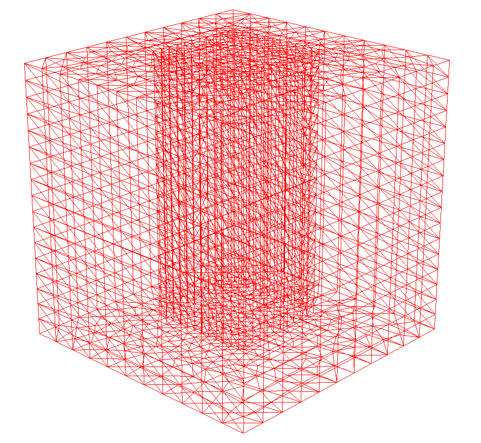
Figure 1: The domain and the mesh. Number of vertices: 2 800. Number of elements (tetrahedra): 14 094. Total number of variables: 20 539.

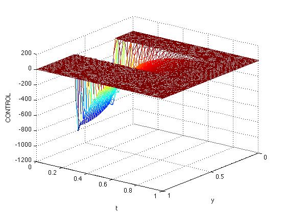
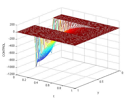
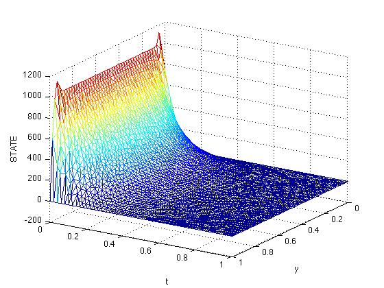
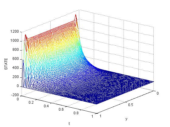
Figure 2: $\omega=(0.2,0.6)$; $y_{0}(\mathbf{x})=1000$. Cuts at $x_{1}=0.28$ and $x_{1}=0.52$ of the control $v_{h}$ (Left) and the state (Right).

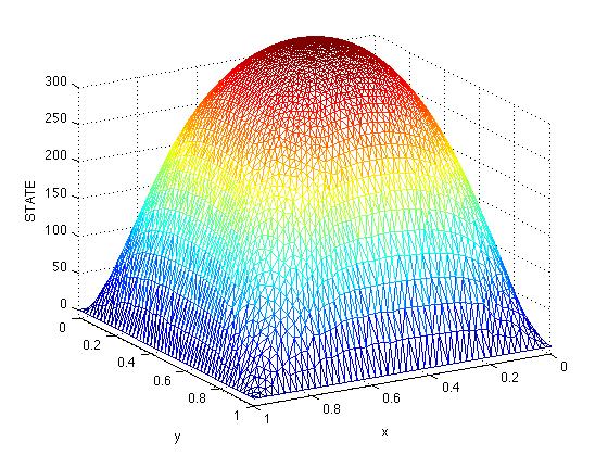
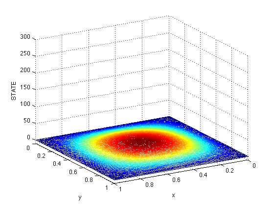
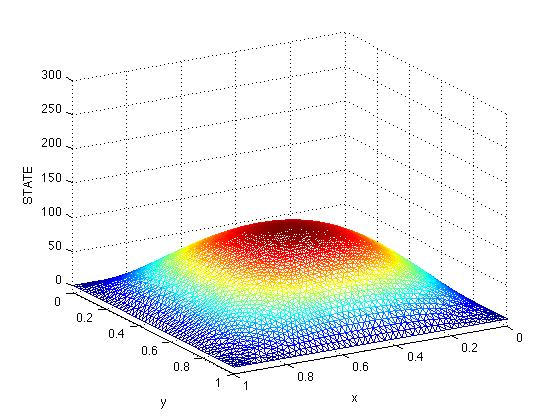
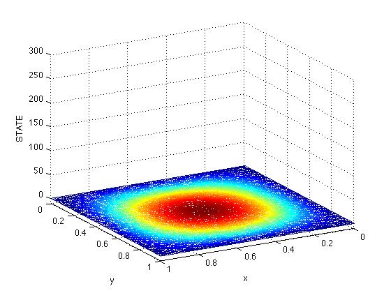
Figure 3: Evolution of the state: $t=0.2$ and $t=0.6$ (Left), $t=0.4$ and $t=0.8$ (Right).

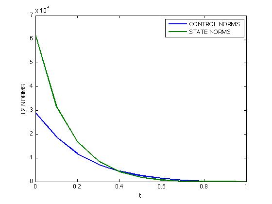
Figure 4: Evolution of the $L^{2}$ norms of the control and the state.

Iterate	Rel. error 1	Rel. error 2
1	$0.225333$	$1.000000$
10	$0.019314$	$0.236549$
20	$0.010068$	$0.065812$
30	$0.005633$	$0.046212$
40	$0.000358$	$0.003397$
50	$0.000117$	$0.001357$

Table 1: The behavior of ALG $1$ for (28).

3 A strategy for the computation of null controls for the Stokes equations

In this Section, we will present a formulation of the null controllability problem for (2) inspired by the same ideas (again, Fursikov-Imanunuvilov’s formulation). Specifically, we will try to solve numerically the problem

$$\left\{\begin{array}[]{llr}\displaystyle\hbox{Minimize }\ J(\mathbf{y},\mathbf{v})={1\over 2}\iint_{Q_{T}}\rho^{2}|\mathbf{y}|^{2}\,d\mathbf{x}\,dt+{1\over 2}\iint_{q_{T}}\rho_{0}^{2}|\mathbf{v}|^{2}\,d\mathbf{x}\,dt\\ \vskip 3.0pt plus 1.0pt minus 1.0pt\cr\displaystyle\hbox{Subject to }\ (\mathbf{y},\mathbf{v})\in\mathcal{S}(\mathbf{y}_{0},T),\end{array}\right.$$ (31)

where $\mathbf{y}_{0}\in\mathbf{H}$, $T>0$, the linear manifold $\displaystyle\mathcal{S}(\mathbf{y}_{0},T)$ is given by

$$\mathcal{S}(\mathbf{y}_{0},T)=\left\{\,(\mathbf{y},\mathbf{v}):\mathbf{v}\in\mathbf{L}^{2}(\omega\times(0,T)),\leavevmode\nobreak\ (\mathbf{y},\mathbf{v})\leavevmode\nobreak\ \hbox{satisfies \eqref{stokes} for some}\leavevmode\nobreak\ \pi\leavevmode\nobreak\ \hbox{and fulfills}\leavevmode\nobreak\ \eqref{null_condition_stokes}\,\right\}$$

and it is again assumed that the weights $\rho$ and $\rho_{0}$ satisfy (9).

We have:

Theorem 6.

For any $\mathbf{y}_{0}\in\mathbf{H}$ and $T>0$, there exists exactly one solution to (31).

Again, this result can be viewed as a consequence of a Carleman inequality. Thus, let us set

$$\mathbf{L}\mathbf{y}:=\mathbf{y}_{t}-\nu\Delta\mathbf{y},\quad\mathbf{L}^{*}\mathbf{p}:=-\mathbf{p}_{t}-\nu\Delta\mathbf{p}$$

and let us introduce the space

$${\mathbf{\Phi}}_{0}=\{\,(\mathbf{p},\sigma):p_{i},\sigma\in C^{2}(\overline{Q}_{T}),\ \nabla\cdot\mathbf{p}\equiv 0,\displaystyle\ p_{i}=0\ \hbox{on}\ \Sigma_{T},\ \int_{\Omega}\!\sigma(\mathbf{x},t)d\mathbf{x}\!=\!0\,\ \forall t\,\}.$$ (32)

Then, one has the following (see [13, 18]):

Proposition 3.

The function $\chi_{0}$ and the associated weights $\rho$, $\rho_{0}$, $\rho_{1}$ and $\rho_{2}$ can be chosen such that there exists $C$, only depending on $\Omega$, $\omega$ and $T$, with the following property:

$$\begin{array}[]{c}\displaystyle\iint_{Q_{T}}\left[\rho_{2}^{-2}(|\mathbf{p}_{t}|^{2}+|\Delta\mathbf{p}|^{2})+\rho_{1}^{-2}|\nabla\mathbf{p}|^{2}+\rho_{0}^{-2}|\mathbf{p}|^{2}+\rho^{-2}|\nabla\sigma|^{2}\right]d\mathbf{x}\,dt\\ \vskip 3.0pt plus 1.0pt minus 1.0pt\cr\displaystyle\leq C\left(\iint_{Q_{T}}\rho^{-2}|\mathbf{L}^{*}\mathbf{p}+\nabla\sigma|^{2}\,d\mathbf{x}\,dt+\iint_{q_{T}}\rho_{0}^{-2}|\mathbf{p}|^{2}\,d\mathbf{x}\,dt\right)\end{array}$$ (33)

for all $(\mathbf{p},\sigma)\in{\mathbf{\Phi}}_{0}$.

Let us introduce the bilinear form

$$\mathbf{m}((\mathbf{p},\sigma),(\mathbf{p}^{\prime},\sigma^{\prime})):=\iint_{Q_{T}}\left[\rho^{-2}(\mathbf{L}^{*}\mathbf{p}+\nabla\sigma)\cdot(\mathbf{L}^{*}\mathbf{p}^{\prime}+\nabla\sigma^{\prime})+1_{\omega}\rho_{0}^{-2}\mathbf{p}\cdot\mathbf{p}^{\prime}\right]d\mathbf{x}\,dt.$$ (34)

In view of the unique continuation property of the Stokes system, $\mathbf{m}(\cdot\,,\cdot)$ is a scalar product in ${\mathbf{\Phi}}_{0}$: if $(\mathbf{p},\sigma)\in{\mathbf{\Phi}}_{0}$, $\mathbf{L}^{*}\mathbf{p}+\nabla\sigma=\mathbf{0}$ in $Q_{T}$ and $\mathbf{p}=\mathbf{0}$ in $q_{T}$, then we have $\mathbf{p}\equiv\mathbf{0}$ and $\sigma\equiv 0$ (note that, in fact, under these circumstances, $\mathbf{p}(\cdot\,,t)$ and $\sigma(\cdot\,,t)$ are analytic for all $t$).

Let ${\mathbf{\Phi}}$ be the completion of ${\mathbf{\Phi}}_{0}$ with respect to this scalar product. As before, ${\mathbf{\Phi}}$ is a Hilbert space, the functions $(\mathbf{p},\sigma)\in{\mathbf{\Phi}}$ satisfy

$$\iint_{Q_{T}}\rho^{-2}|\mathbf{L}^{*}\mathbf{p}+\nabla\sigma|^{2}\,d\mathbf{x}\,dt+\iint_{q_{T}}\rho_{0}^{-2}|\mathbf{p}|^{2}\,d\mathbf{x}\,dt<+\infty$$ (35)

and, from Proposition 3 and a density argument, we also have (35) for any $(\mathbf{p},\sigma)\in{\mathbf{\Phi}}$.

We also see from Proposition 3 that

$$\begin{array}[]{c}\displaystyle{\mathbf{\Phi}}=\{\,(\mathbf{p},\sigma):p_{i},\sigma,\partial_{t}p_{i},\partial_{x_{j}}p_{i},\partial_{x_{j}}\sigma,\partial_{x_{j}x_{k}}p_{i}\in L^{2}(0,T-\delta;L^{2}(\Omega))\ \forall\delta>0,\\ \vskip 3.0pt plus 1.0pt minus 1.0pt\cr\displaystyle\eqref{finite-rhs}\ \hbox{holds},\ \nabla\cdot\mathbf{p}\equiv 0\ \hbox{in}\ Q_{T},\ p_{i}=0\ \hbox{on}\ \Sigma_{T},\ \int_{\Omega}\sigma(\mathbf{x},t)\,d\mathbf{x}=0\,\ \forall t\,\}\end{array}$$ (36)

and, in particular, any $(\mathbf{p},\sigma)\in{\mathbf{\Phi}}$ satisfies $\mathbf{p}\in C^{0}([0,T-\delta];\mathbf{V})$ for all $\delta>0$ and

$$\|\mathbf{p}(\cdot\,,0)\|_{\mathbf{V}}\leq C\,\mathbf{m}((\mathbf{p},\sigma),(\mathbf{p},\sigma))^{1/2}\quad\forall(\mathbf{p},\sigma)\in{\mathbf{\Phi}}.$$ (37)

The following result is proved in [13]:

Theorem 7.

Let the weights $\rho$ and $\rho_{0}$ be chosen as in Proposition 3. Let $(\mathbf{y},\mathbf{v})$ be the unique solution to (31). Then one has

$$\mathbf{y}=\rho^{-2}(L^{*}\mathbf{p}+\nabla\sigma),\quad\mathbf{v}=-\rho_{0}^{-2}\bigl{.}\mathbf{p}\bigr{|}_{\omega\times(0,T)},$$ (38)

where $(\mathbf{p},\sigma)$ is the solution to the following variational equality in ${\mathbf{\Phi}}$:

$$\left\{\begin{array}[]{l}\displaystyle\iint_{Q_{T}}\left(\rho^{-2}(\mathbf{L}^{*}\mathbf{p}+\nabla\sigma)\cdot(\mathbf{L}^{*}\mathbf{p}^{\prime}+\nabla\sigma^{\prime})+\rho_{0}^{-2}\mathbf{p}\cdot\mathbf{p}^{\prime}1_{\omega}\right)d\mathbf{x}\,dt=\displaystyle\int_{\Omega}\mathbf{y}_{0}(\mathbf{x})\cdot\mathbf{p}^{\prime}(\mathbf{x},0)\,d\mathbf{x}\\ \vskip 3.0pt plus 1.0pt minus 1.0pt\cr\displaystyle\forall(\mathbf{p}^{\prime},\sigma^{\prime})\in{\mathbf{\Phi}};\ (\mathbf{p},\sigma)\in{\mathbf{\Phi}}.\end{array}\right.$$ (39)

Once more, (39) can be viewed as the weak formulation of a (non-scalar) boundary-value problem for a PDE that is fourth-order in $\mathbf{x}$ and second-order in $t$. Indeed, arguing as in Section 2, we can easily deduce that $(\mathbf{p},\sigma)$ satisfies, together with some $\pi\in\mathcal{D}^{\prime}(Q_{T})$, the following:

$$\left\{\begin{array}[]{lcl}\mathbf{L}(\rho^{-2}(\mathbf{L}^{*}\mathbf{p}+\nabla\sigma))+\nabla\pi+1_{\omega}\rho_{0}^{-2}\mathbf{p}=0&\text{in}&Q_{T},\\ \vskip 3.0pt plus 1.0pt minus 1.0pt\cr\nabla\cdot(\rho^{-2}(\mathbf{L}^{*}\mathbf{p}+\nabla\sigma))=0,\leavevmode\nobreak\ \nabla\cdot\mathbf{p}=0&\text{in}&Q_{T},\\ \vskip 3.0pt plus 1.0pt minus 1.0pt\cr\mathbf{p}=\textbf{0},\ \ \rho^{-2}(\mathbf{L}^{*}\mathbf{p}+\nabla\sigma)=\mathbf{0}&\text{on}&\Sigma_{T},\\ \vskip 3.0pt plus 1.0pt minus 1.0pt\cr\bigl{.}\rho^{-2}(\mathbf{L}^{*}\mathbf{p}+\nabla\sigma)\bigr{|}_{t=0}=\mathbf{y}_{0},\ \ \bigl{.}\rho^{-2}(\mathbf{L}^{*}\mathbf{p}+\nabla\sigma)\bigr{|}_{t=T}=\mathbf{0}&\text{in}&\Omega.\end{array}\right.$$ (40)

By setting

$$\langle\ell_{0},(\mathbf{p},\sigma)\rangle:=\int_{\Omega}\mathbf{y}_{0}(\mathbf{x})\cdot\mathbf{p}(\mathbf{x},0)\,d\mathbf{x},$$ (41)

it is found that (39) can be rewritten in the form

$$\mathbf{m}((\mathbf{p},\sigma),((\mathbf{p}^{\prime},\sigma^{\prime}))=\langle\ell_{0},(\mathbf{p}^{\prime},\sigma^{\prime})\rangle\displaystyle\quad\forall(\mathbf{p}^{\prime},\sigma^{\prime})\in{\mathbf{\Phi}};\ (\mathbf{p},\sigma)\in{\mathbf{\Phi}}.$$ (42)

Thus, if ${\mathbf{\Phi}}_{h}$ denotes a finite dimensional subspace of ${\mathbf{\Phi}}$, a natural approximation of (42) is the following:

$$\mathbf{m}((\mathbf{p}_{h},\sigma_{h}),((\mathbf{p}^{\prime}_{h},\sigma^{\prime}_{h}))=\langle\ell_{0},(\mathbf{p}^{\prime}_{h},\sigma^{\prime}_{h})\rangle\displaystyle\quad\forall(\mathbf{p}^{\prime}_{h},\sigma^{\prime}_{h})\in{\mathbf{\Phi}}_{h};\ (\mathbf{p}_{h},\sigma_{h})\in{\mathbf{\Phi}}_{h}.$$ (43)

However, the couples $(\mathbf{p},\sigma)\in{\mathbf{\Phi}}$ satisfy several properties that make it considerably difficult to construct explicitly finite dimensional spaces ${\mathbf{\Phi}}_{h}\subset{\mathbf{\Phi}}$. These are the following:

• As in Section 2, since $\rho^{-1}(\mathbf{L}^{*}\mathbf{p}+\nabla\sigma)$ must belong to $\mathbf{L}^{2}(Q_{T})$ and $\bigl{.}\rho_{0}^{-1}\mathbf{p}\bigr{|}_{q_{T}}$ must belong to $\mathbf{L}^{2}(q_{T})$, the $p_{i}$ must possess first-order time derivatives and up to second-order spatial derivatives in $L^{2}_{\rm loc}(Q_{T})$. As before, this means that, in practice, the functions in ${\mathbf{\Phi}}_{h}$ must be $C^{0}$ in $(\mathbf{x},t)$ and $C^{1}$ in $\mathbf{x}$.

• We now have $\nabla\cdot\mathbf{p}\equiv 0$. It is not simple at all to give explicit expressions of zero (or approximately zero) divergence functions associated to a triangulation of $Q_{T}$ with this regularity.

The second inconvenient is classical in computational fluid dynamics when one considers incompressible fluids. As in many other works, it will be overcome by introducing additional “pressure-like” multipliers; see Section 3.2. On the other hand, the first difficulty will be circumvented as in Section 2, by introducing new variables and associated multipliers and eliminating all the second-order derivatives in the formulation.

In the following Sections, we will present several mixed problems connected to (42).

More precisely, in Sections 3.1 and 3.4, we consider mixed formulations where the constraint $\nabla\cdot\mathbf{p}\equiv 0$ is preserved. Accordingly, we only introduce one additional variable $\mathbf{z}$ and one multiplier, related to the identity $\mathbf{z}=L^{*}\mathbf{p}+\nabla\sigma$. Contrarily, Sections 3.2, 3.3 and 3.5 deal with other different formulations where the zero-divergence condition is not imposed and, therefore, another multiplier appears.

3.1 A first mixed formulation of (42)

Arguing as in the case of the heat equation and introducing the variable

$$\mathbf{z}=\mathbf{L}^{*}\mathbf{p}+\nabla\sigma,$$

we see that (42) is equivalent to:

$$\left\{\begin{array}[]{l}\vskip 3.0pt plus 1.0pt minus 1.0pt\cr\displaystyle\mathbf{a}((\mathbf{z},\mathbf{p},\sigma),(\mathbf{z}^{\prime},\mathbf{p}^{\prime},\sigma^{\prime}))+\mathbf{b}((\mathbf{z}^{\prime},\mathbf{p}^{\prime},\sigma^{\prime}),\mathbf{\lambda})=\langle\mbox{\boldmath{$\ell$}},(\mathbf{z}^{\prime},\mathbf{p}^{\prime},\sigma^{\prime})\rangle,\\ \vskip 3.0pt plus 1.0pt minus 1.0pt\cr\displaystyle\mathbf{b}((\mathbf{z},\mathbf{p},\sigma),\mathbf{\lambda}^{\prime})=0,\\ \vskip 3.0pt plus 1.0pt minus 1.0pt\cr\displaystyle\quad\forall((\mathbf{z}^{\prime},\mathbf{p}^{\prime},\sigma^{\prime}),\mathbf{\lambda}^{\prime})\in\mathbf{Z}\times{\mathbf{\Phi}}\times\mathbf{\Lambda};\ ((\mathbf{z},\mathbf{p},\sigma),\mathbf{\lambda})\in\mathbf{Z}\times{\mathbf{\Phi}}\times\mathbf{\Lambda},\end{array}\right.$$ (44)

where

$$\mathbf{Z}=\mathbf{L}^{2}(\rho^{-1};Q_{T}),\quad\mathbf{\Lambda}=\mathbf{L}^{2}(\rho;Q_{T})$$

and the bilinear forms $\mathbf{a}(\cdot\,,\cdot)$ and $\mathbf{b}(\cdot\,,\cdot)$ are given by

$$\mathbf{a}((\mathbf{z},\mathbf{p},\sigma),(\mathbf{z}^{\prime},\mathbf{p}^{\prime},\sigma^{\prime})):=\iint_{Q_{T}}\left(\rho^{-2}\mathbf{z}\cdot\mathbf{z}^{\prime}+\rho_{0}^{-2}\mathbf{p}\cdot\mathbf{p}^{\prime}1_{\omega}\right)\,d\mathbf{x}\,dt$$

and

$$\mathbf{b}((\mathbf{z},\mathbf{p},\sigma),\mathbf{\lambda}):=\displaystyle\iint_{Q_{T}}\left[\mathbf{z}-(\mathbf{L}^{*}\mathbf{p}+\nabla\sigma)\right]\cdot\mathbf{\lambda}\,d\mathbf{x}\,dt\\$$ (45)

and the linear form $\ell$ is given by

$$\langle\mbox{\boldmath{$\ell$}},(\mathbf{z},\mathbf{p},\sigma)\rangle:=\int_{\Omega}\mathbf{y}_{0}(\mathbf{x})\cdot\mathbf{p}(\mathbf{x},0)\,d\mathbf{x}.$$

3.2 A second mixed formulation of (42)

As we have said, numerical difficulties are found when we try to introduce finite element approximations ($C^{1}$ in space, $C^{0}$ in time) of the space ${\mathbf{\Phi}}$, where the $(\mathbf{p},\sigma)$ satisfy $\nabla\cdot\mathbf{p}\equiv 0$. Accordingly, before approximating, we will reformulate (39) as a new mixed system involving a multiplier associated to this constraint.

Let us introduce

$$\tilde{\mathbf{\Phi}}_{0}=\{\,(\mathbf{p},\sigma):p_{i},\sigma\in C^{2}(\overline{Q}_{T}),\displaystyle\ p_{i}=0\ \hbox{on}\ \Sigma_{T},\ \int_{\Omega}\sigma(\mathbf{x},t)d\mathbf{x}=0\,\ \forall t\,\}.$$ (46)

We have the following Carleman estimates for the couples in $\tilde{\mathbf{\Phi}}_{0}$:

Proposition 4.

There exist weights $\rho$, $\rho_{0}$ and $\rho_{*}$ and a constant $C$ only depending on $\Omega$, $\omega$ and $T$, with the following property:

$$\begin{array}[]{l}\displaystyle\iint_{Q_{T}}\rho_{0}^{-2}|\mathbf{p}|^{2}d\mathbf{x}\,dt+\|\mathbf{p}(\cdot,0)\|^{2}_{\mathbf{V}^{\prime}}\leq C\left(\iint_{Q_{T}}\rho_{*}^{-2}|\mathbf{L}^{*}\mathbf{p}+\nabla\sigma|^{2}\,d\mathbf{x}\,dt+\iint_{q_{T}}\rho_{0}^{-2}|\mathbf{p}|^{2}\,d\mathbf{x}\,dt\right.\\ \vskip 3.0pt plus 1.0pt minus 1.0pt\cr\displaystyle\phantom{\iint_{Q_{T}}\rho_{0}^{-2}|\mathbf{p}|^{2}d\mathbf{x}\,dt+\|\mathbf{p}(\cdot,0)\|^{2}_{\mathbf{V}^{\prime}}\leq C}\left.+\iint_{Q_{T}}|\nabla\cdot\mathbf{p}|^{2}\,d\mathbf{x}\,dt\right)\end{array}$$ (47)

for all $(\mathbf{p},\sigma)\in\tilde{\mathbf{\Phi}}_{0}$.

Proof.

The proof follows easily by splitting $(\mathbf{p},\sigma)\in\tilde{\mathbf{\Phi}}_{0}$ in the form

$$(\mathbf{p},\sigma)=(\tilde{\mathbf{p}},\tilde{\sigma})+(\hat{\mathbf{p}},\hat{\sigma})$$

where $(\hat{\mathbf{p}},\hat{\sigma})$ solves the linear problem

$$\left\{\begin{array}[]{lcl}\mathbf{L}^{*}\hat{\mathbf{p}}+\nabla\hat{\sigma}=\mathbf{f}&\text{in}&Q_{T},\\ \vskip 3.0pt plus 1.0pt minus 1.0pt\cr\nabla\cdot\hat{\mathbf{p}}=0&\text{in}&Q_{T},\\ \vskip 3.0pt plus 1.0pt minus 1.0pt\cr\hat{\mathbf{p}}=\mathbf{0}&\text{on}&\Sigma_{T},\\ \vskip 3.0pt plus 1.0pt minus 1.0pt\cr\hat{\mathbf{p}}(\cdot,T)=\mathbf{p}(\cdot,T)&\text{in}&\Omega\end{array}\right.$$ (48)

with $\mathbf{f}:=\mathbf{L}^{*}\mathbf{p}+\nabla\sigma$ and $(\tilde{\mathbf{p}},\tilde{\sigma})$ solves the linear problem

$$\left\{\begin{array}[]{lcl}\mathbf{L}^{*}\tilde{\mathbf{p}}+\nabla\tilde{\sigma}=\mathbf{0}&\text{in}&Q_{T},\\ \vskip 3.0pt plus 1.0pt minus 1.0pt\cr\nabla\cdot\tilde{\mathbf{p}}=\nabla\cdot\mathbf{p}&\text{in}&Q_{T},\\ \vskip 3.0pt plus 1.0pt minus 1.0pt\cr\tilde{\mathbf{p}}=\mathbf{0}&\text{on}&\Sigma_{T},\\ \vskip 3.0pt plus 1.0pt minus 1.0pt\cr\tilde{\mathbf{p}}(\cdot\,,T)=\mathbf{0}&\text{in}&\Omega.\end{array}\right.$$ (49)

In view of the Carleman estimates (33) for $(\hat{\mathbf{p}},\hat{\sigma})$, we have

$$\begin{array}[]{c}\displaystyle\iint_{Q_{T}}\rho_{0}^{-2}|\hat{\mathbf{p}}|^{2}\,d\mathbf{x}\,dt+\|\mathbf{p}(\cdot\,,0)\|_{\mathbf{V}}^{2}\leq C\left(\iint_{Q_{T}}\rho^{-2}|\mathbf{f}|^{2}\,d\mathbf{x}\,dt+\iint_{q_{T}}\rho_{0}^{-2}|\hat{\mathbf{p}}|^{2}\,d\mathbf{x}\,dt\right).\end{array}$$

On the other hand, $(\tilde{\mathbf{p}},\tilde{\sigma})$ solves (49) in the sense of transposition, that is,

$$\langle\tilde{\mathbf{p}},\mbox{\boldmath{$\psi$}}\rangle_{\mathbf{L}^{2}(Q_{T}),\mathbf{L}^{2}(Q_{T})}+\langle\tilde{\mathbf{p}}(\cdot,0),\mathbf{u}_{0}\rangle_{\mathbf{V}^{\prime},\mathbf{V}}=-\iint_{Q_{T}}(\nabla\cdot\mathbf{p})\,h\,d\mathbf{x}\,dt,$$

for all $(\mbox{\boldmath{$\psi$}},\mathbf{u}_{0})\in\mathbf{L}^{2}(Q_{T})\times\mathbf{V}$, where $(\mathbf{u},h)$ is the unique strong solution to

$$\left\{\begin{array}[]{lcl}\mathbf{L}\mathbf{u}+\nabla h=\mbox{\boldmath{$\psi$}}&\text{in}&Q_{T},\\ \vskip 3.0pt plus 1.0pt minus 1.0pt\cr\nabla\cdot\mathbf{u}=\mathbf{0}&\text{in}&Q_{T},\\ \vskip 3.0pt plus 1.0pt minus 1.0pt\cr\mathbf{u}=\mathbf{0}&\text{on}&\Sigma_{T},\\ \vskip 3.0pt plus 1.0pt minus 1.0pt\cr\mathbf{u}(\cdot\,,0)=\mathbf{u}_{0}&\text{in}&\Omega.\end{array}\right.$$

Consequently, we can argue as in [23] and deduce that

$$\|\tilde{\mathbf{p}}\|^{2}_{\mathbf{L}^{2}(Q_{T})}+\|\tilde{\mathbf{p}}(\cdot,0)\|^{2}_{\mathbf{V}^{\prime}}\leq C\,\|\nabla\cdot\mathbf{p}\|^{2}_{L^{2}(Q_{T})}.$$

Now, putting together the estimates for $(\hat{\mathbf{p}},\hat{\sigma})$ and $(\tilde{\mathbf{p}},\tilde{\sigma})$, we are easily led easily to (47). ∎

Let us introduce the bilinear form

$$\tilde{\mathbf{m}}((\mathbf{p},\sigma),(\mathbf{p}^{\prime},\sigma^{\prime})):=\mathbf{m}((\mathbf{p},\sigma),(\mathbf{p}^{\prime},\sigma^{\prime}))+\iint_{Q_{T}}(\nabla\cdot\mathbf{p})(\nabla\cdot\mathbf{p}^{\prime})\,d\mathbf{x}\,dt.$$

Again, in view of the unique continuation property of the Stokes system, $\tilde{\mathbf{m}}(\cdot\,,\cdot)$ is a scalar product in $\tilde{\mathbf{\Phi}}_{0}$.

Let $\tilde{\mathbf{\Phi}}$ be the completion of $\tilde{\mathbf{\Phi}}_{0}$ with respect to this scalar product. As before, $\tilde{\mathbf{\Phi}}$ is a Hilbert space, the functions $(\mathbf{p},\sigma)\in\tilde{\mathbf{\Phi}}$ satisfy

$$\iint_{Q_{T}}\rho^{-2}|\mathbf{L}^{*}\mathbf{p}+\nabla\sigma|^{2}\,d\mathbf{x}\,dt+\iint_{q_{T}}\rho_{0}^{-2}|\mathbf{p}|^{2}\,d\mathbf{x}\,dt+\iint_{Q_{T}}|\nabla\cdot\mathbf{p}|^{2}d\mathbf{x}\,dt<+\infty$$ (50)

and, from Proposition 4 and a density argument, we also have (47) for all $(\mathbf{p},\sigma)\in\tilde{\mathbf{\Phi}}$.

On the other hand, any $(\mathbf{p},\sigma)\in\tilde{\mathbf{\Phi}}$ satisfies

$$\rho_{0}^{-1}\mathbf{p}\in\mathbf{L}^{2}(Q_{T}),\quad\mathbf{p}(\cdot,0)\in\mathbf{V}^{\prime}$$

and

$$\|\mathbf{p}(\cdot\,,0)\|_{\mathbf{V}^{\prime}}^{2}\leq C\,\tilde{\mathbf{m}}((\mathbf{p},\sigma),(\mathbf{p},\sigma))\quad\forall(\mathbf{p},\sigma)\in\tilde{\mathbf{\Phi}}.$$ (51)

By setting

$$\langle\mbox{\boldmath{$\tilde{\ell}$}},(\mathbf{p},\sigma)\rangle:=\langle\mathbf{p}(\cdot,0),\mathbf{y}_{0}\rangle_{\mathbf{V}^{\prime},\mathbf{V}}$$ (52)

thanks to (51), we have that $\tilde{\ell}$ is continuous on $\tilde{\mathbf{\Phi}}$.

Let us introduce the space

$$\tilde{M}=\{\,\mu\in L^{2}(Q_{T}):\int_{\Omega}\mu(\mathbf{x},t)\,d\mathbf{x}=0\,\leavevmode\nobreak\ \hbox{a.e.}\,\}$$

and the following reformulation of (42):

$$\left\{\begin{array}[]{l}\displaystyle\tilde{\mathbf{m}}((\mathbf{p},\sigma),(\mathbf{p}^{\prime},\sigma^{\prime}))+\iint_{Q_{T}}\left(\nabla\cdot\mathbf{p}^{\prime}\right)\mu\,d\mathbf{x}\,dt=\langle\tilde{\mbox{\boldmath{$\ell$}}},(\mathbf{p},\sigma)\rangle,\\ \vskip 3.0pt plus 1.0pt minus 1.0pt\cr\displaystyle\iint_{Q_{T}}\left(\nabla\cdot\mathbf{p}\right)\mu^{\prime}\,d\mathbf{x}\,dt=0,\\ \vskip 3.0pt plus 1.0pt minus 1.0pt\cr\displaystyle\qquad\forall(\mathbf{p}^{\prime},\sigma^{\prime},\mu^{\prime})\in\tilde{\mathbf{\Phi}}\times\tilde{M};\ (\mathbf{p},\sigma,\mu)\in\tilde{\mathbf{\Phi}}\times\tilde{M}.\end{array}\right.$$ (53)

Once more, notice that the definitions of $\tilde{\mathbf{\Phi}}$ and $\tilde{M}$ are the appropriate to keep all the terms in (53) meaningful.

Let the bilinear forms $\tilde{\mathbf{a}}(\cdot\,,\cdot)$ and $\tilde{\mathbf{b}}(\cdot\,,\cdot)$ be given by

$$\tilde{\mathbf{a}}((\mathbf{p},\sigma),(\mathbf{p}^{\prime},\sigma^{\prime})):=\mathbf{m}((\mathbf{p},\sigma),(\mathbf{p}^{\prime},\sigma^{\prime}))$$

and

$$\tilde{\mathbf{b}}(\mathbf{p},\sigma,\mu):=\iint_{Q_{T}}\left(\nabla\cdot\mathbf{p}\right)\mu\,d\mathbf{x}\,dt.$$

Then, $\tilde{\mathbf{a}}(\cdot\,,\cdot)$ and $\tilde{\mathbf{b}}(\cdot\,,\cdot)$ are well-defined and continuous and (53) reads:

$$\left\{\begin{array}[]{l}\displaystyle\tilde{\mathbf{a}}((\mathbf{p},\sigma),(\mathbf{p}^{\prime},\sigma^{\prime}))+\tilde{\mathbf{b}}(\mathbf{p}^{\prime},\sigma^{\prime},\mu)=\langle\mbox{\boldmath{$\tilde{\ell}$}},(\mathbf{p}^{\prime},\sigma^{\prime})\rangle,\\ \vskip 3.0pt plus 1.0pt minus 1.0pt\cr\displaystyle\tilde{\mathbf{b}}((\mathbf{p},\sigma),\mu^{\prime})=0,\\ \vskip 3.0pt plus 1.0pt minus 1.0pt\cr\displaystyle\qquad\forall(\mathbf{p}^{\prime},\sigma^{\prime},\mu^{\prime})\in\tilde{\mathbf{\Phi}}\times\tilde{M};\ (\mathbf{p},\sigma,\mu)\in\tilde{\mathbf{\Phi}}\times\tilde{M}.\end{array}\right.$$ (54)

One has the following:

Proposition 5.

There exists exactly one solution to (54). Furthermore, (42) and (54) are equivalent problems in the following sense:

1. If $(\mathbf{p},\sigma,\mu)$ solves (54), then $(\mathbf{p},\sigma)$ solves (42).

2. If $(\mathbf{p},\sigma)$ solves (42), there exists $\mu\in\tilde{M}$ such that $(\mathbf{p},\sigma,\mu)$ solves (54).

Proof.

Let us set

$$\tilde{\mathbf{\Psi}}:=\{\,(\mathbf{p},\sigma)\in\tilde{\mathbf{\Phi}}:\tilde{\mathbf{b}}(\mathbf{p},\sigma,\mu)=0\quad\forall\mu\in\tilde{M}\,\}.$$

We will check that

• $\tilde{\mathbf{a}}(\cdot\,,\cdot)$ is coercive in $\tilde{\mathbf{\Psi}}$.

• $\tilde{\mathbf{b}}(\cdot\,,\cdot)$ satisfies the usual “inf-sup” condition in $\tilde{\mathbf{\Phi}}\times\tilde{M}$.

The proofs of these assertions are straightforward. Indeed, we have $\tilde{\mathbf{\Psi}}={\mathbf{\Phi}}$ (the completion of ${\mathbf{\Phi}}_{0}$ with respect to $\mathbf{m}(\cdot,\cdot)$, see (34)). Thus,

$$\begin{array}[]{lll}\displaystyle\tilde{\mathbf{a}}((\mathbf{p},\sigma),(\mathbf{p},\sigma))=\displaystyle\mathbf{m}((\mathbf{p},\sigma),(\mathbf{p},\sigma))=\tilde{\mathbf{m}}((\mathbf{p},\sigma),(\mathbf{p},\sigma))\quad\forall(\mathbf{p},\sigma)\in\tilde{\mathbf{\Psi}}\end{array}$$

and this proves that $\tilde{\mathbf{a}}(\cdot\,,\cdot)$ is coercive in $\tilde{\mathbf{\Psi}}$.

On the other hand, the “inf-sup” condition is a consequence of the fact that, for any $\mu\in\tilde{M}$, there exists $(\mathbf{p},\sigma)\in\tilde{\mathbf{\Phi}}$ such that

$$\tilde{\mathbf{b}}(\mathbf{p},\sigma,\mu)=\|\mu\|^{2}_{\tilde{M}}\quad\hbox{and}\quad\|(\mathbf{p},\sigma)\|_{\tilde{\mathbf{\Phi}}}\leq C\|\mu\|_{\tilde{M}}.$$ (55)

This can be seen as follows: for any fixed $\mu\in\tilde{M}$, let $(\mathbf{p},\sigma)$ be the solution to

$$\mathbf{L}^{*}\mathbf{p}+\nabla\sigma=\mathbf{0}\,\leavevmode\nobreak\ \textrm{in}\,\leavevmode\nobreak\ Q_{T},\quad\nabla\cdot\mathbf{p}=\mu\,\leavevmode\nobreak\ \textrm{in}\,\leavevmode\nobreak\ Q_{T},\quad\mathbf{p}=\mathbf{0}\,\leavevmode\nobreak\ \textrm{ on }\leavevmode\nobreak\ \,\Sigma_{T},\quad\mathbf{p}(\cdot,T)=\mathbf{0}\,\leavevmode\nobreak\ \textrm{in}\,\leavevmode\nobreak\ \Omega;$$

then $\mathbf{p}$ belongs to $\mathbf{L}^{2}(Q_{T})$ and

$$\|\mathbf{p}\|_{\mathbf{L}^{2}(Q_{T})}\leq C\|\mu\|_{L^{2}(Q_{T})}$$ (56)

(see [23]). Therefore, it is lear that (55) also holds. ∎

3.3 A third mixed reformulation of (54) with an additional multiplier

As in Section 3.1, introducing the variable

$$\mathbf{z}:=\mathbf{L}^{*}\mathbf{p}+\nabla\sigma,$$

we observe that (54) is equivalent to:

$$\left\{\begin{array}[]{l}\displaystyle\hat{\mathbf{a}}((\mathbf{z},\mathbf{p},\sigma),(\mathbf{z}^{\prime},\mathbf{p}^{\prime},\sigma^{\prime}))+\hat{\mathbf{b}}((\mathbf{z}^{\prime},\mathbf{p}^{\prime},\sigma^{\prime}),(\mbox{\boldmath{$\lambda$}},\mu))=\langle\mbox{\boldmath{$\hat{\ell}$}},(\mathbf{z}^{\prime},\mathbf{p}^{\prime},\sigma^{\prime})\rangle,\\ \vskip 3.0pt plus 1.0pt minus 1.0pt\cr\displaystyle\hat{\mathbf{b}}((\mathbf{z},\mathbf{p},\sigma),(\mbox{\boldmath{$\lambda$}}^{\prime},\mu^{\prime}))=0,\\ \vskip 3.0pt plus 1.0pt minus 1.0pt\cr\displaystyle\qquad\forall((\mathbf{z}^{\prime},\mathbf{p}^{\prime},\sigma^{\prime}),(\mbox{\boldmath{$\lambda$}}^{\prime},\mu^{\prime}))\in\mathbf{Z}\times\tilde{\mathbf{\Phi}}\times\mathbf{\Lambda}\times\tilde{M};\ ((\mathbf{z},\mathbf{p},\sigma),(\mbox{\boldmath{$\lambda$}},\mu))\in\mathbf{Z}\times\tilde{\mathbf{\Phi}}\times\mathbf{\Lambda}\times\tilde{M},\end{array}\right.$$ (57)

where the bilinear forms $\hat{\mathbf{a}}(\cdot\,,\cdot)$ and $\hat{\mathbf{b}}(\cdot\,,\cdot)$ are given by

$$\hat{\mathbf{a}}((\mathbf{z},\mathbf{p},\sigma),(\mathbf{z}^{\prime},\mathbf{p}^{\prime},\sigma^{\prime})):=\iint_{Q_{T}}\left(\rho^{-2}\mathbf{z}\cdot\mathbf{z}^{\prime}+\rho_{0}^{-2}\mathbf{p}\cdot\mathbf{p}^{\prime}1_{\omega}\right)\,d\mathbf{x}\,dt$$

and

$$\hat{\mathbf{b}}((\mathbf{z},\mathbf{p},\sigma),(\mbox{\boldmath{$\lambda$}},\mu)):=\displaystyle\iint_{Q_{T}}\left[\mathbf{z}-(\mathbf{L}^{*}\mathbf{p}+\nabla\sigma)\right]\cdot\mbox{\boldmath{$\lambda$}}\,d\mathbf{x}\,dt+\iint_{Q_{T}}\left(\nabla\cdot\mathbf{p}\right)\mu\,d\mathbf{x}\,dt\\$$ (58)

and the linear form $\hat{\ell}$ is given by

$$\langle\mbox{\boldmath{$\hat{\ell}$}},(\mathbf{z},\mathbf{p},\sigma)\rangle:=\int_{\Omega}\mathbf{y}_{0}(\mathbf{x})\cdot\mathbf{p}(\mathbf{x},0)\,d\mathbf{x}.$$

Now, the following holds:

Proposition 6.

There exists exactly one solution to (57). Furthermore, (54) and (57) are equivalent problems in the following sense:

1. If $((\mathbf{z},\mathbf{p},\sigma),(\mbox{\boldmath{$\lambda$}},\mu))$ solves (57), then $(\mathbf{p},\sigma,\mu)$ solve (54).

2. If $(\mathbf{p},\sigma,\mu)$ solves (54), there exists $\mbox{\boldmath{$\lambda$}}\in\mathbf{\Lambda}$ such that $((\mathbf{z},\mathbf{p},\sigma),(\mbox{\boldmath{$\lambda$}},\mu))$, with

   $$\mathbf{z}:=\mathbf{L}^{*}\mathbf{p}+\nabla\sigma,$$

   solves (57).

Proof.

Let us introduce the space

$$\hat{\mathbf{\Psi}}=\{\,(\mathbf{z},\mathbf{p},\sigma)\in\mathbf{Z}\times\tilde{\mathbf{\Phi}}:\hat{\mathbf{b}}((\mathbf{z},\mathbf{p},\sigma),(\mbox{\boldmath{$\lambda$}},\mu))=0\quad\forall(\mbox{\boldmath{$\lambda$}},\mu)\in\mathbf{\Lambda}\times\tilde{M}\,\}$$

and, as before, let us check that

• $\hat{\mathbf{a}}(\cdot\,,\cdot)$ is coercive in $\hat{\mathbf{\Psi}}$.

• $\hat{\mathbf{b}}(\cdot\,,\cdot)$ satisfies the usual “inf-sup” condition in $(\mathbf{Z}\times\tilde{\mathbf{\Phi}})\times(\mathbf{\Lambda}\times\tilde{M})$.

Again, the proofs of these assertions are easy. Indeed, for any $(\mathbf{z},\mathbf{p},\sigma)\in\hat{\mathbf{\Psi}}$, $\mathbf{z}=\mathbf{L}^{*}\mathbf{p}+\nabla\sigma$ and $\nabla\cdot\mathbf{p}=0$ and, therefore,

$$\hat{\mathbf{a}}((\mathbf{z},\mathbf{p},\sigma),(\mathbf{z},\mathbf{p},\sigma))= \leavevmode\nobreak\ \iint_{Q_{T}}\left(\rho^{-2}|\mathbf{z}|^{2}+\rho_{0}^{-2}|\mathbf{p}|^{2}\,1_{\omega}\right)\,d\mathbf{x}\,dt$$

$$= \leavevmode\nobreak\ {1\over 2}\|(\mathbf{z},\mathbf{p},\sigma)\|^{2}_{\mathbf{Z}\times\tilde{\mathbf{\Phi}}}+{1\over 2}\iint_{Q_{T}}\rho_{0}^{-2}|\mathbf{p}|^{2}1_{\omega}\,d\mathbf{x}\,dt$$

$$\geq \leavevmode\nobreak\ {1\over 2}\|(\mathbf{z},\mathbf{p},\sigma)\|^{2}_{\mathbf{Z}\times\tilde{\mathbf{\Phi}}},$$

whence $\hat{\mathbf{a}}(\cdot\,,\cdot)$ is coercive in $\hat{\mathbf{\Psi}}$.

On the other hand, the “inf-sup” condition is a consequence of the fact that, for any $(\mbox{\boldmath{$\lambda$}},\mu)\in\mathbf{\Lambda}\times\tilde{M}$, there exists $(\mathbf{z},\mathbf{p},\sigma)\in\mathbf{Z}\times\tilde{\mathbf{\Phi}}$ such that

$$\hat{\mathbf{b}}((\mathbf{z},\mathbf{p},\sigma),(\mbox{\boldmath{$\lambda$}},\mu))=\|(\mbox{\boldmath{$\lambda$}},\mu)\|^{2}_{\mathbf{\Lambda}\times\tilde{M}}\quad\hbox{and}\quad\|(\mathbf{z},\mathbf{p},\sigma)\|_{\mathbf{Z}\times\tilde{\mathbf{\Phi}}}\leq C\|(\mbox{\boldmath{$\lambda$}},\mu)\|_{\mathbf{\Lambda}\times\tilde{M}}.$$ (59)

This time, the argument is as follows: for any fixed $(\mbox{\boldmath{$\lambda$}},\mu)\in\hat{\mathbf{Y}}$, let $(\mathbf{p},\sigma)$ be the solution to

$$\mathbf{L}^{*}\mathbf{p}+\nabla\sigma=\mathbf{0}\,\leavevmode\nobreak\ \textrm{in}\,\leavevmode\nobreak\ Q_{T},\quad\nabla\cdot\mathbf{p}=\mu\,\leavevmode\nobreak\ \textrm{in}\,\leavevmode\nobreak\ Q_{T},\quad\mathbf{p}=0\,\leavevmode\nobreak\ \textrm{ on }\leavevmode\nobreak\ \,\Sigma_{T},\quad\mathbf{p}(\cdot,T)=\mathbf{0}\,\leavevmode\nobreak\ \textrm{in}\,\leavevmode\nobreak\ \Omega;$$

then $\mathbf{p}$ belongs to $\mathbf{L}^{2}(Q_{T})$ and

$$\|\mathbf{p}\|_{\mathbf{L}^{2}(Q_{T})}\leq C\|\mu\|_{L^{2}(Q_{T})}.$$ (60)

Taking $\mathbf{z}=\rho^{2}\mbox{\boldmath{$\lambda$}}$, one arrives easily at (59). ∎

3.4 Another formulation related to (44)

Let us introduce the spaces

$${\mathbf{\Phi}}^{*}:=\leavevmode\nobreak \{\,(\mathbf{p},\sigma):\,\iint_{Q_{T}}\left[\rho_{2}^{-2}|\mathbf{p}_{t}|^{2}+\rho_{1}^{-2}|\nabla\mathbf{p}|^{2}+\rho_{0}^{-2}|\mathbf{p}|^{2}+\rho^{-2}|\nabla\sigma|^{2}\right]d\mathbf{x}\,dt<+\infty,$$

$$\,\leavevmode\nobreak\ \nabla\cdot\mathbf{p}\equiv 0,\leavevmode\nobreak\ \mathbf{p}=\mathbf{0}\ \text{ on }\ \Sigma_{T}\,\},$$

$$\mathbf{\Lambda}^{*}:=\leavevmode\nobreak \{\,\mbox{\boldmath{$\lambda$}}:\ \iint_{Q_{T}}\left[\rho_{2}^{2}|\mbox{\boldmath{$\lambda$}}|^{2}+\rho_{1}^{2}|\nabla\mbox{\boldmath{$\lambda$}}|^{2}\right]d\mathbf{x}\,dt<+\infty,\leavevmode\nobreak\ \mbox{\boldmath{$\lambda$}}=\mathbf{0}\ \text{ on }\ \Sigma_{T}\,\},$$

the bilinear forms $\mathbf{a}^{*}(\cdot\,,\cdot)$ and $\mathbf{b}^{*}(\cdot\,,\cdot)$, with

$$\mathbf{a}^{*}((\mathbf{z},\mathbf{p},\sigma),(\mathbf{z}^{\prime},\mathbf{p}^{\prime},\sigma^{\prime})):=\iint_{Q_{T}}\left(\rho^{-2}\mathbf{z}\cdot\mathbf{z}^{\prime}+\rho_{0}^{-2}\mathbf{p}\cdot\mathbf{p}^{\prime}1_{\omega}\right)\,d\mathbf{x}\,dt$$

and

$$\mathbf{b}^{*}((\mathbf{z},\mathbf{p},\sigma),\mbox{\boldmath{$\lambda$}}):=\displaystyle\iint_{Q_{T}}\left\{\left[\mathbf{z}+\mathbf{p}_{t}-\nabla\sigma\right]\cdot\mbox{\boldmath{$\lambda$}}-\nu\nabla\mathbf{p}\cdot\nabla\mbox{\boldmath{$\lambda$}}\right\}\,d\mathbf{x}\,dt\\$$

and the linear form $\ell^{*}$, with

$$\langle\mbox{\boldmath{$\ell^{*}$}},(\mathbf{z},\mathbf{p},\sigma)\rangle:=\int_{\Omega}\mathbf{y}_{0}(\mathbf{x})\cdot\mathbf{p}(\mathbf{x},0)\,d\mathbf{x}.$$

The bilinear form $\mathbf{b}^{*}(\cdot,\cdot)$ appears when we integrate by parts the second–order terms in $\mathbf{b}(\cdot,\cdot)$, see (45). Accordingly, at least formally, we can reformulate (44) as follows:

$$\left\{\begin{array}[]{l}\displaystyle\mathbf{a}^{*}((\mathbf{z},\mathbf{p},\sigma),(\mathbf{z}^{\prime},\mathbf{p}^{\prime},\sigma^{\prime}))+\mathbf{b}^{*}((\mathbf{z}^{\prime},\mathbf{p}^{\prime},\sigma^{\prime}),\mbox{\boldmath{$\lambda$}}^{\prime})=\langle\mbox{\boldmath{$\ell^{*}$}},(\mathbf{z}^{\prime},\mathbf{p}^{\prime},\sigma^{\prime})\rangle,\\ \vskip 3.0pt plus 1.0pt minus 1.0pt\cr\displaystyle\mathbf{b}^{*}((\mathbf{z},\mathbf{p},\sigma),\mbox{\boldmath{$\lambda$}})=0,\\ \vskip 3.0pt plus 1.0pt minus 1.0pt\cr\displaystyle\qquad\forall((\mathbf{z}^{\prime},\mathbf{p}^{\prime},\sigma^{\prime}),\mbox{\boldmath{$\lambda$}}^{\prime})\in\mathbf{Z}\times{\mathbf{\Phi}}^{*}\times\mathbf{\Lambda}^{*};\ ((\mathbf{z},\mathbf{p},\sigma),\mbox{\boldmath{$\lambda$}})\in\mathbf{Z}\times{\mathbf{\Phi}}^{*}\times\mathbf{\Lambda}^{*}.\end{array}\right.$$ (61)

This can be viewed as a new mixed formulation of (42). However, that these two problems are equivalent in the sense of Propositions 5 and 6 is, at present, an open question.

3.5 A fifth (and final) mixed formulation

Finally, let us introduce the space

$$\overline{{\mathbf{\Phi}}}:=\leavevmode\nobreak \{\,(\mathbf{p},\sigma):\,\,\iint_{Q_{T}}\!\!\!\!\left[\rho_{2}^{-2}|\mathbf{p}_{t}|^{2}\!+\!\rho_{1}^{-2}|\nabla\mathbf{p}|^{2}\!+\!\rho_{0}^{-2}|\mathbf{p}|^{2}\!+\!|\nabla\cdot\mathbf{p}|^{2}\!+\!\rho^{-2}|\nabla\sigma|^{2}\right]\,d\mathbf{x}\,dt<+\infty,$$

$$\mathbf{p}=\mathbf{0}\ \text{ on }\ \Sigma_{T}\,\},$$

the bilinear forms $\overline{\mathbf{a}}(\cdot\,,\cdot)$ and $\overline{\mathbf{b}}(\cdot\,,\cdot)$, with

$$\overline{\mathbf{a}}((\mathbf{z},\mathbf{p},\sigma),(\mathbf{z}^{\prime},\mathbf{p}^{\prime},\sigma^{\prime})):=\iint_{Q_{T}}\left(\rho^{-2}\mathbf{z}\cdot\mathbf{z}^{\prime}+\rho_{0}^{-2}\mathbf{p}\cdot\mathbf{p}^{\prime}1_{\omega}\right)\,d\mathbf{x}\,dt$$

and

$$\overline{\mathbf{b}}((\mathbf{z},\mathbf{p},\sigma),(\mathbf{\lambda},\mu)):=\displaystyle\iint_{Q_{T}}\left\{\left[\mathbf{z}+\mathbf{p}_{t}-\nabla\sigma\right]\cdot\mbox{\boldmath{$\lambda$}}-\nu\nabla\mathbf{p}\cdot\nabla\mbox{\boldmath{$\lambda$}}\right\}\,d\mathbf{x}\,dt+\iint_{Q_{T}}\left(\nabla\cdot\mathbf{p}\right)\mu\,d\mathbf{x}\,dt\\$$

and the linear form $\overline{\mbox{\boldmath{$\ell$}}}$, with

$$\langle\overline{\mbox{\boldmath{$\ell$}}},(\mathbf{z},\mathbf{p},\sigma)\rangle:=\int_{\Omega}\mathbf{y}_{0}(\mathbf{x})\cdot\mathbf{p}(\mathbf{x},0)\,d\mathbf{x}.$$

In accordance with (61), it can be accepted that, at least formally, (57) possesses the following reformulation:

$$\left\{\begin{array}[]{l}\displaystyle\overline{\mathbf{a}}((\mathbf{z},\mathbf{p},\sigma),(\mathbf{z}^{\prime},\mathbf{p}^{\prime},\sigma^{\prime}))+\overline{\mathbf{b}}((\mathbf{z}^{\prime},\mathbf{p}^{\prime},\sigma^{\prime}),(\mathbf{\lambda},\mu))=\langle\overline{\mbox{\boldmath{$\ell$}}},(\mathbf{z}^{\prime},\mathbf{p}^{\prime},\sigma^{\prime})\rangle,\\ \vskip 3.0pt plus 1.0pt minus 1.0pt\cr\displaystyle\overline{\mathbf{b}}((\mathbf{z},\mathbf{p},\sigma),(\mathbf{\lambda}^{\prime},\mu^{\prime}))=0,\\ \vskip 3.0pt plus 1.0pt minus 1.0pt\cr\displaystyle\qquad\forall((\mathbf{z}^{\prime},\mathbf{p}^{\prime},\sigma^{\prime}),(\mbox{\boldmath{$\lambda$}}^{\prime},\mu^{\prime}))\in\mathbf{Z}\times\overline{{\mathbf{\Phi}}}\times\mathbf{\Lambda}\times M;\ ((\mathbf{z},\mathbf{p},\sigma),(\mbox{\boldmath{$\lambda$}},\mu))\in\mathbf{Z}\times\overline{{\mathbf{\Phi}}}\times\mathbf{\Lambda}\times M.\end{array}\right.$$ (62)

Remark 3.

The previous mixed formulations possess several relevant properties:

• By constructing finite dimensional subspaces of ${\mathbf{\Phi}}$, we are led to standard mixed approximations of (44). But this is not a simple task: recall that, in order to have $(\mathbf{p},\sigma)\in{\mathbf{\Phi}}$, we need (among other things) $\mathbf{L}^{*}\mathbf{p}+\nabla\sigma\in\mathbf{L}^{2}(\rho^{-1};Q_{T})$ and $\nabla\cdot\mathbf{p}=0$.

• Contrarily, it is relatively easy to construct numerically efficient finite dimensional subspaces of $\tilde{\mathbf{\Phi}}$, for instance, based on the Bell triangle or the Bogner-Fox-Schmidt rectangle. Consequently, we can get finite element approximations of (54) for which, furthermore, a convergence analysis can be performed.

• The same can be said for (57). In this case, the fact that the variable $\mathbf{z}$ appears explicitly is useful for a direct computation of an approximation of the state.

• The mixed formulations (61) and (62) share an advantageous characteristic: they can be approximated in a rather standard way by $C^{0}$ finite elements since, after integration by parts, no second-order spatial derivative appears. Unfortunately, up to our knowledge, it is unknown whether or not they are well posed. More precisely, the proof of the “inf-sup” condition is open and, moreover, the well-posedness of their associated discrete versions is not clear.

3.6 A numerical approximation of (62) (without justification)

Let us conserve the notation in Section 2.4.

For any couple of integers $m,n\geq 1$, we will set

$$\begin{array}[]{l}\vskip 3.0pt plus 1.0pt minus 1.0pt\cr\displaystyle\overline{\mathbf{Z}}_{h}(m,n):=\{\,\mathbf{z}_{h}\in\mathbf{C}^{0}(\overline{Q}_{\kappa,T}):\mathbf{z}_{h}|_{K}\in(\mathbb{P}_{m,\mathbf{x}}\otimes\mathbb{P}_{n,t})(K)\ \ \forall K\in{\mathcal{Q}}_{h}\,\},\\ \vskip 3.0pt plus 1.0pt minus 1.0pt\cr\displaystyle\overline{\mathbf{V}}_{h}(m,n):=\{\,\mathbf{p}_{h}\in\overline{\mathbf{Z}}_{h}(m,n):\mathbf{p}_{h}=\mathbf{0}\ \hbox{ on }\ \Sigma_{T}\,\},\\ \vskip 3.0pt plus 1.0pt minus 1.0pt\cr\displaystyle\overline{M}_{h}(m,n):=\{\,\sigma_{h}\in C^{0}(\overline{Q}_{\kappa,T}):\sigma_{h}|_{K}\in(\mathbb{P}_{m,\mathbf{x}}\otimes\mathbb{P}_{n,t})(K)\ \ \forall K\in{\mathcal{Q}}_{h}\,\}.\end{array}$$

Then, $\overline{\mathbf{Z}}_{h}(m,n)$ and $\overline{\mathbf{V}}_{h}(m,n)$ are finite dimensional subspaces of the Hilbert space $\mathbf{H}^{1}(Q_{\kappa,T})$. Moreover, $\overline{\mathbf{V}}_{h}(m,n)\times\overline{M}_{h}(m,n)\subset\overline{{\mathbf{\Phi}}}$, $\overline{\mathbf{V}}_{h}(m,n)\subset\overline{\mathbf{\Lambda}}$ and $\overline{M}_{h}(m,n)\subset\tilde{M}$. Therefore, for any $m$, $n$, $m^{\prime}$, $n^{\prime}$, $m^{\prime\prime}$, $n^{\prime\prime}$, $m^{\prime\prime\prime}$, $n^{\prime\prime\prime}$, $m^{\prime\prime\prime\prime}$, $n^{\prime\prime\prime\prime}\geq 1$, we can define

$$\overline{\mathbf{X}}_{h}:=\overline{\mathbf{Z}}_{h}(m,n)\times\overline{\mathbf{V}}_{h}(m^{\prime},n^{\prime})\times\overline{M}_{h}(m^{\prime\prime},n^{\prime\prime})\hbox{ and }\overline{\mathbf{Y}}_{h}:=\overline{\mathbf{V}}_{h}(m^{\prime\prime\prime},n^{\prime\prime\prime})\times\overline{M}_{h}(m^{\prime\prime\prime\prime},n^{\prime\prime\prime\prime}),$$

that are finite dimensional subspaces of $\mathbf{Z}\times\overline{{\mathbf{\Phi}}}$ and $\mathbf{\Lambda}\times M$, respectively.

The following mixed approximation of (62) makes sense:

$$\left\{\begin{array}[]{l}\displaystyle\overline{\mathbf{a}}((\mathbf{z}_{h},(\mathbf{p}_{h},\sigma_{h})),(\mathbf{z}^{\prime}_{h},(\mathbf{p}^{\prime}_{h},\sigma^{\prime}_{h})))+\overline{\mathbf{b}}((\mathbf{z}^{\prime}_{h},(\mathbf{p}^{\prime}_{h},\sigma^{\prime}_{h})),(\mathbf{\lambda}_{h},\mu_{h}))=\langle\overline{\mbox{\boldmath{$\ell$}}},(\mathbf{z}^{\prime}_{h},(\mathbf{p}^{\prime}_{h},\sigma^{\prime}_{h}))\rangle,\\ \vskip 3.0pt plus 1.0pt minus 1.0pt\cr\displaystyle\overline{\mathbf{b}}((\mathbf{z}_{h},(\mathbf{p}_{h},\sigma_{h})),(\mathbf{\lambda}^{\prime}_{h},\mu^{\prime}_{h}))=0,\\ \vskip 3.0pt plus 1.0pt minus 1.0pt\cr\displaystyle\qquad\forall((\mathbf{z}^{\prime}_{h},(\mathbf{p}^{\prime}_{h},\sigma^{\prime}_{h})),(\mbox{\boldmath{$\lambda$}}^{\prime}_{h},\mu^{\prime}_{h}))\in\overline{\mathbf{X}}_{h}\times\overline{\mathbf{Y}}_{h};\ ((\mathbf{z}_{h},(\mathbf{p}_{h},\sigma_{h})),(\mbox{\boldmath{$\lambda$}}_{h},\mu_{h}))\in\overline{\mathbf{X}}_{h}\times\overline{\mathbf{Y}}_{h}.\end{array}\right.$$ (63)

3.7 A numerical experiment

This Section deals with some numerical results. We have solved (63) with the following data: $\Omega=(0,1)\times(0,1)$, $\omega=(0.2,0.6)\times(0.2,0.6)$, $T=1$, $K_{1}=1$, $K_{2}=2$, $\chi_{0}=\chi_{0}^{(0.5,0.5)}$ (as in Section 2); $\nu=1$, $\mathbf{y}_{0}(\mathbf{x})\equiv(M,0)$, with $M=1000$.

Again, the computations have been performed with the software Freefem++, using $P_{2}$-Lagrange approximations in $(\mathbf{x},t)$ for all the variables. Th domain and the mesh are depicted in Fig. 1. The linear system in (63) has been solved with the Arrow-Hurwicz algorithm, where we have taken $r=0.01$ and $s=0.1$. The convergence of this algorithm is illustrated in Table 2, where the first and the second relative errors are given by

$${\|(\mathbf{z}^{(k+1)}_{h},\mathbf{p}^{(k+1)}_{h},\sigma^{(k+1)}_{h})-(\mathbf{z}^{(k)}_{h},\mathbf{p}^{(k)}_{h},\sigma^{(k)}_{h})\|_{\mathbf{L}^{2}(Q_{T})}\over\|(\mathbf{z}^{(k+1)}_{h},\mathbf{p}^{(k+1)}_{h},\sigma^{(k+1)}_{h})\|_{\mathbf{L}^{2}(Q_{T})}}$$

and

$${\|(\mathbf{\lambda}^{(k+1)}_{h},\mu^{(k+1)}_{h})-(\mathbf{\lambda}^{(k)}_{h},\mu^{(k)}_{h})\|_{\mathbf{L}^{2}(Q_{T})}\over\|(\mathbf{\lambda}^{(k+1)}_{h},\mu^{(k+1)}_{h})\|_{\mathbf{L}^{2}(Q_{T})}}\,.$$

The computed control and state are displayed in Fig. 5–8.

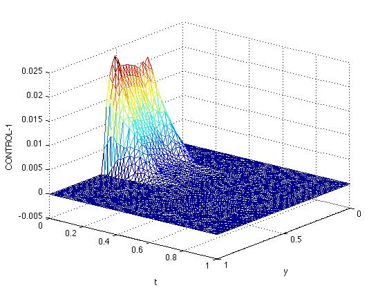
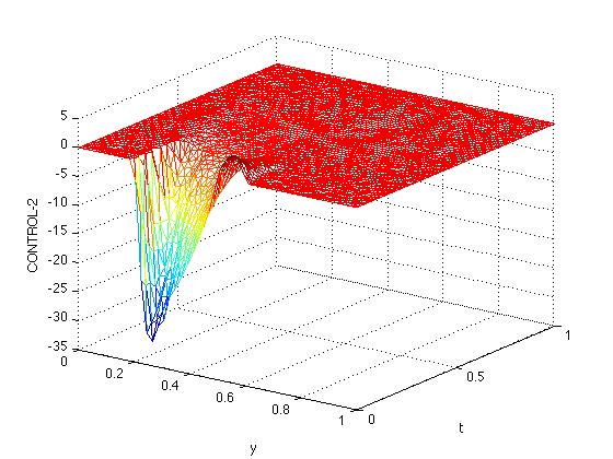
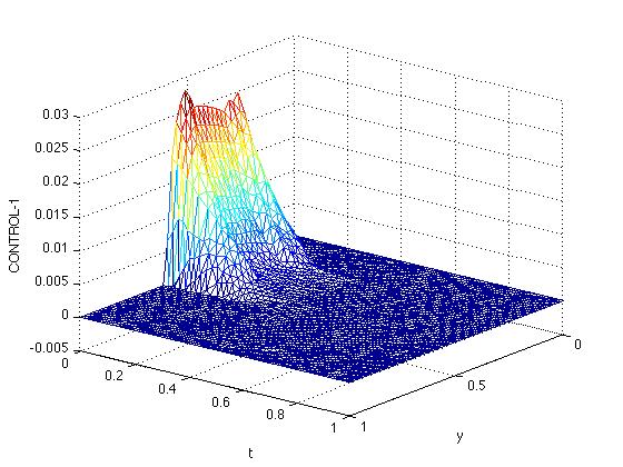
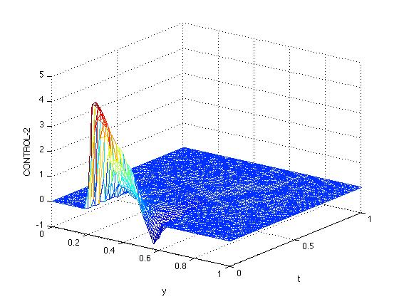
Figure 5: $\omega=(0.2,0.6)$; $\mathbf{y}_{0}(\mathbf{x})=(1000,0)$. Cuts of $v_{1,h}$ and $10^{10}v_{2,h}$ at $x_{1}=0.28$ (Left) and $x_{1}=0.52$ (Right).

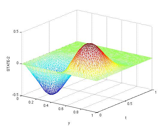
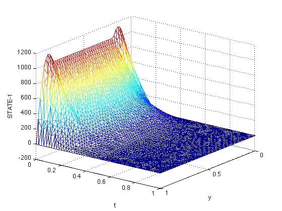
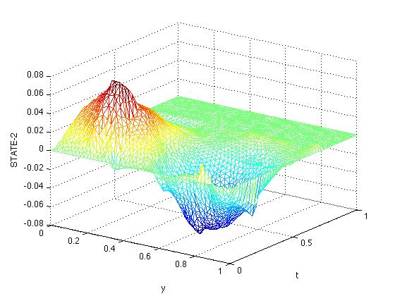
Figure 6: $\omega=(0.2,0.6)$; $\mathbf{y}_{0}(\mathbf{x})=(1000,0)$. Cuts of $y_{1,h}$ and $10^{10}y_{2,h}$ at $x_{1}=0.28$ (Left) and $x_{1}=0.52$ (Right).

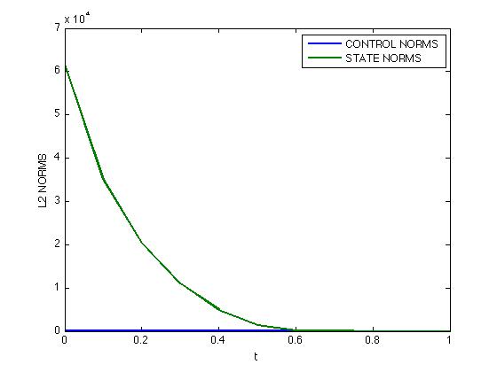
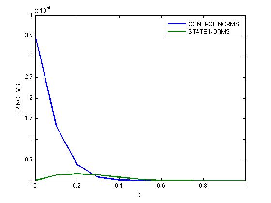
Figure 7: Evolution of the $L^{2}$ norms of the first and second components of the control and the state.

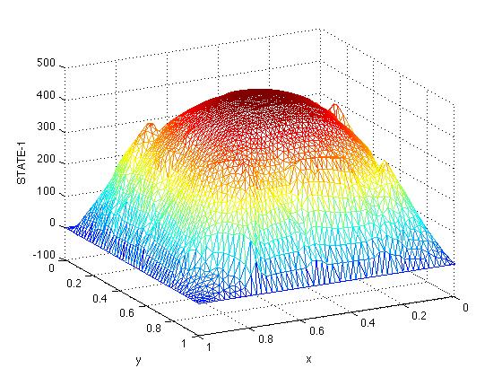
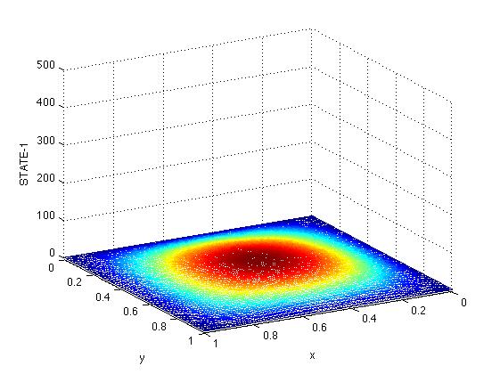
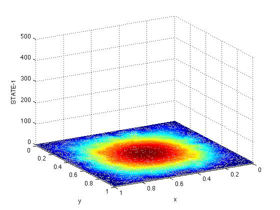
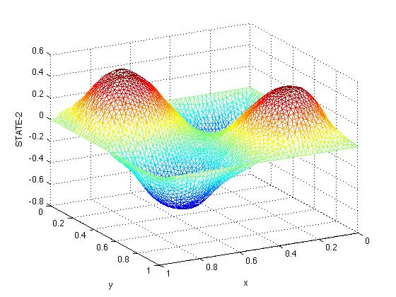
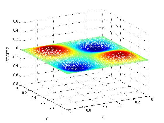
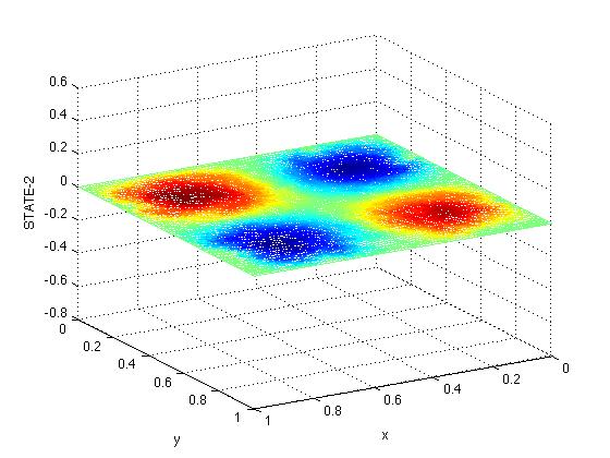
Figure 8: Evolution of the state at times $t=0.2$, $t=0.5$ and $t=0.8$. Cuts of $y_{1,h}$ (Left) and $10^{10}y_{2,h}$ (Right).

Iterate	Rel. error 1	Rel. error 2
1	$0.659686$	$0.202439$
10	$0.063864$	$0.106203$
20	$0.016147$	$0.076083$
30	$0.008874$	$0.046212$
40	$0.000464$	$0.001397$
50	$0.000206$	$0.000762$

Table 2: The behavior of the Arrow-Hurwicz algorithm for (63).

4 An application : numerical local exact controllability to the trajectories of the Navier-Stokes equations

In this Section, we will present a numerical method for the computation of a solution to the local exact controllability problem to the trajectories of (3). This controllability property was proved in [9] under suitable regularity assumptions on the trajectories. More precisely, we have to assume that the trajectory satisfies

$$\overline{\mathbf{y}}\in L^{2}(0,T;D(\mathbf{A}))\cap C^{0}([0,T];\mathbf{V})\cap\mathbf{L}^{\infty}(Q_{T}),\quad\overline{\mathbf{y}}_{t}\in L^{2}\bigl{(}0,T;\mathbf{H}\bigl{)},$$ (64)

where $D(\mathbf{A}):=\mathbf{H}^{2}(\Omega)\cap\mathbf{V}$ is the domain of the usual Stokes operator $\mathbf{A}$; see also [18] for a previous result.

4.1 A fixed-point algorithm and a mixed formulation

First of all, let us rewrite the local exact controllability to the trajectories as a null controllability problem. To do this, let us put $\mathbf{y}=\overline{\mathbf{y}}+\mathbf{u}$ and $\pi=\overline{\pi}+q$ and let us use (3). Taking into account that $(\overline{\mathbf{y}},\overline{\pi})$ solves (6), we find:

$$\left\{\begin{array}[]{lcl}\mathbf{u}_{t}-\nu\Delta\mathbf{u}+(\mathbf{u}\cdot\nabla)\overline{\mathbf{y}}+((\overline{\mathbf{y}}+\mathbf{u})\cdot\nabla)\mathbf{u}+\nabla q=\mathbf{v}1_{\omega}&\hbox{in}&Q_{T},\\ \nabla\cdot\mathbf{u}=0&\hbox{in}&Q_{T},\\ \mathbf{u}=\mathbf{0}&\hbox{on}&\Sigma_{T},\\ \mathbf{u}(0)=\mathbf{u}_{0}:=\mathbf{y}_{0}-\overline{\mathbf{y}}_{0}&\hbox{in}&\Omega.\end{array}\right.$$ (65)

This way, we have reduced our problem to a local null controllability result for the solution $(\mathbf{u},q)$ to the nonlinear problem (65).

Let us suppose that $\mathbf{u}_{0}\in D(\mathbf{A}^{\sigma})$, with $1/2<\sigma<1$ ($\mathbf{A}^{\sigma}$ is the fractional power of the Stokes operator) and let us introduce the fixed-point mapping $F:\mathbf{W}\mapsto\mathbf{W}$, where

$$\mathbf{W}:=\left\{\,\mathbf{u}\in\mathbf{L}^{\infty}(Q_{T}):\nabla\cdot\mathbf{u}=0\hbox{ in }Q_{T},\ \mathbf{u}\cdot\mathbf{n}=0\hbox{ on }\Sigma_{T}\,\right\}.$$

Here, for any $\mathbf{w}\in\mathbf{W}$, $\mathbf{u}=F(\mathbf{w})$ is, together with some $\mathbf{v}$ and $q$, the unique solution to the extremal problem

$$\left\{\begin{array}[]{l}\displaystyle\hbox{Minimize }\ J(\mathbf{w};\mathbf{u},\mathbf{v})={1\over 2}\iint_{Q_{T}}\rho^{2}|\mathbf{u}|^{2}\,d\mathbf{x}\,dt+{1\over 2}\iint_{q_{T}}\rho_{0}^{2}|\mathbf{v}|^{2}\,d\mathbf{x}\,dt\\ \vskip 3.0pt plus 1.0pt minus 1.0pt\cr\displaystyle\hbox{Subject to }\ \mathbf{v}\in L^{2}(q_{T}),\ (\mathbf{u},q,\mathbf{v})\ \text{satisfies}\ \eqref{N-S-REFOR-LL},\end{array}\right.$$ (66)

where (67) reads as follows:

$$\left\{\begin{array}[]{lcl}\mathbf{u}_{t}-\nu\Delta\mathbf{u}+(\mathbf{u}\cdot\nabla)\overline{\mathbf{y}}+((\overline{\mathbf{y}}+\mathbf{w})\cdot\nabla)\mathbf{u}+\nabla q=\mathbf{v}1_{\omega}&\hbox{in}&Q_{T},\\ \nabla\cdot\mathbf{u}=0&\hbox{in}&Q_{T},\\ \mathbf{u}=\mathbf{0}&\hbox{on}&\Sigma_{T},\\ \mathbf{u}(0)=\mathbf{u}_{0}&\hbox{in}&\Omega.\end{array}\right.$$ (67)

It is again assumed that the weights $\rho$ and $\rho_{0}$ satisfy (9).

We have:

Theorem 8.

For any $\mathbf{u}_{0}\in D(\mathbf{A}^{\sigma})$ and $T>0$, there exists exactly one solution to (66)-(67).

This can be regarded as a consequence of the following Carleman inequality for Oseen systems (the proof can be found in [19]):

Proposition 7.

For all $R>0$, the function $\chi_{0}$ and the associated weights $\rho$, $\rho_{0}$ and $\rho_{1}$ furnished by Proposition 1 can be chosen such that, for some $C$, only depending on $\Omega$, $\omega$, $T$ and $R$, and for all $\mathbf{w}\in\mathbf{W}$ with $\|\mathbf{w}\|_{\mathbf{L}^{\infty}(Q_{T})}\leq R$, one has:

$$\begin{array}[]{c}\displaystyle\iint_{Q_{T}}\!\!\!\!\!\left(\rho_{1}^{-2}|\nabla\mathbf{p}|^{2}\!+\!\rho_{0}^{-2}|\mathbf{p}|^{2}\!+\!\rho^{-2}|\nabla\sigma|^{2}\right)d\mathbf{x}\,dt\!\leq\!C\!\left(\iint_{Q_{T}}\!\!\!\!\!\rho^{-2}|\mathbf{M}^{*}\mathbf{p}\!+\!\nabla\sigma|^{2}\,d\mathbf{x}\,dt\!+\!\!\iint_{q_{T}}\!\!\!\!\rho_{0}^{-2}|\mathbf{p}|^{2}\,d\mathbf{x}\,dt\right)\end{array}$$ (68)

for all $(\mathbf{p},\sigma)\in{\mathbf{\Phi}}_{0}$. Here, we have used the notation

$$\quad\mathbf{M}^{*}\mathbf{p}=-\mathbf{p}_{t}-\nu\Delta\mathbf{p}-\nabla\mathbf{p}\,(\overline{\mathbf{y}}+\mathbf{w})-\nabla\mathbf{p}^{t}\,\overline{\mathbf{y}},\quad\mathbf{M}\mathbf{u}=\mathbf{u}_{t}-\nu\Delta\mathbf{u}+(\mathbf{u}\cdot\nabla)\overline{\mathbf{y}}+((\overline{\mathbf{y}}+\mathbf{w})\cdot\nabla)\mathbf{u}.$$

For any $\mathbf{w}\in\mathbf{W}$, we will denote by $\mathbf{m}(\mathbf{w};\,\cdot\,,\,\cdot\,)$ the following associated bilinear form on ${\mathbf{\Phi}}_{0}$:

$$\mathbf{m}(\mathbf{w};(\mathbf{p},\sigma),(\mathbf{p}^{\prime},\sigma^{\prime})):=\iint_{Q_{T}}\left(\rho^{-2}(\mathbf{M}^{*}\mathbf{p}+\nabla\sigma)\cdot(\mathbf{M}^{*}\mathbf{p}^{\prime}+\nabla\sigma^{\prime})+1_{\omega}\rho_{0}^{-2}\mathbf{p}\cdot\mathbf{p}^{\prime}\right)\,d\mathbf{x}\,dt;$$

recall that ${\mathbf{\Phi}}_{0}$ is given in (32).

This bilinear form is a scalar product in ${\mathbf{\Phi}}_{0}$. Let us denote by ${\mathbf{\Phi}}^{\mathbf{w}}$ the corresponding completion. Then, for a good choice of $\rho$ and $\rho_{0}$ (the same as above), the solution to (66) can be characterized by the identities

$$\mathbf{u}=\rho^{-2}(\mathbf{M}^{*}\mathbf{p}_{\mathbf{w}}+\nabla\sigma_{\mathbf{w}}),\quad\mathbf{v}=-\rho_{0}^{-2}\bigl{.}\mathbf{p}_{\mathbf{w}}\bigr{|}_{q_{T}},$$ (69)

where $(\mathbf{p}_{\mathbf{w}},\sigma_{\mathbf{w}})$ is the solution to a variational equality in the Hilbert space ${\mathbf{\Phi}}^{\mathbf{w}}$:

$$\left\{\begin{array}[]{l}\mathbf{m}(\mathbf{w};(\mathbf{p}_{\mathbf{w}},\sigma_{\mathbf{w}}),(\mathbf{p}^{\prime},\sigma^{\prime}))=\displaystyle\!\!\int_{\Omega}\mathbf{u}_{0}(\mathbf{x})\cdot\mathbf{p}^{\prime}(\mathbf{x},0)\,d\mathbf{x}\\ \vskip 3.0pt plus 1.0pt minus 1.0pt\cr\displaystyle\forall(\mathbf{p}^{\prime},\sigma^{\prime})\in{\mathbf{\Phi}}^{\mathbf{w}};\ (\mathbf{p}_{\mathbf{w}},\sigma_{\mathbf{w}})\in{\mathbf{\Phi}}^{\mathbf{w}}.\end{array}\right.$$ (70)

Remark 4.

Note that, in view of (68), for any fixed $R>0$, the weights indicated in Proposition (7) lead to a family of norms $\mathbf{m}(\mathbf{w};\cdot,\cdot)^{1/2}$ that are equivalent as long as $\|\mathbf{w}\|_{\mathbf{L}^{\infty}(Q_{T})}\leq R$. Consequently, the associated spaces ${\mathbf{\Phi}}^{\mathbf{w}}$ are the same for all $\mathbf{w}$ with $\|\mathbf{w}\|_{\mathbf{L}^{\infty}(Q_{T})}\leq R$. $\Box$

In order to solve the null controllability problem for (65), it suffices to find a solution to the fixed-point equation

$$\mathbf{u}=F(\mathbf{u}),\quad\mathbf{u}\in\mathbf{W}.$$ (71)

Moreover, in view of the results in [15], if $\mathbf{u}_{0}$ is small enough, $F$ is well defined and possesses at least one fixed-point.

Consequently, a natural strategy is to use the following algorithm:

ALG 2 (Fixed-point):

1. Choose $\mathbf{u}^{0}\in\mathbf{W}$.

2. Then, for given $n\!\geq\!0$ and $\mathbf{u}^{n}\!\in\!\mathbf{W}$, compute $\mathbf{u}^{n\!+\!1}\!=\!F(\mathbf{u}^{n})$, i.e. find the unique solution $(\mathbf{u}^{n+1},\mathbf{v}^{n+1})$ to the extremal problem

   $$\left\{\begin{array}[]{l}\displaystyle\hbox{Minimize }\ J(\mathbf{u}^{n};\mathbf{u}^{n+1},\mathbf{v}^{n+1})=\rho^{2}|\mathbf{u}^{n+1}|^{2}\,d\mathbf{x}\,dt+{1\over 2}\iint_{q_{T}}\rho_{0}^{2}|\mathbf{v}^{n+1}|^{2}\,d\mathbf{x}\,dt\\ \vskip 3.0pt plus 1.0pt minus 1.0pt\cr\displaystyle\hbox{Subject to }\ \mathbf{v}^{n+1}\in L^{2}(q_{T}),\ (\mathbf{u}^{n+1},q^{n+1},\mathbf{v}^{n+1})\ \text{satisfies}\ \eqref{N-S-REFOR-L-n},\end{array}\right.$$ (72)

   where (73) is the following

   $$\left\{\begin{array}[]{lll}\mathbf{u}^{n+1}_{t}-\nu\Delta\mathbf{u}^{n+1}+(\mathbf{u}^{n+1}\cdot\nabla)\overline{\mathbf{y}}+((\overline{\mathbf{y}}+\mathbf{u}^{n})\cdot\nabla)\mathbf{u}^{n+1}+\nabla q^{n+1}=\mathbf{v}^{n+1}1_{\omega}&\hbox{in}&Q_{T},\\ \nabla\cdot\mathbf{u}^{n+1}=0&\hbox{in}&Q_{T},\\ \mathbf{u}^{n+1}=\mathbf{0}&\hbox{on}&\Sigma_{T},\\ \mathbf{u}^{n+1}(0)=\mathbf{u}_{0}&\hbox{in}&\Omega.\end{array}\right.$$ (73)

This is a classical fixed-point method for (71). We start from a prescribed state $\mathbf{u}^{0}$ and, then, we solve a null controllability problem for a linear parabolic system at each step. This way, we produce a sequence $\{\mathbf{u}^{n},\mathbf{v}^{n}\}$ that is expected to converge to a solution to the null controllability problem (65).

For the numerical solution of the problems (72)–(73), we can apply arguments similar to those in Sections 3.5 and 3.6. Thus, a suitable mixed formulation is:

$$\left\{\begin{array}[]{l}\displaystyle\overline{\mathbf{a}}((\mathbf{z},\mathbf{p},\sigma),(\mathbf{z}^{\prime},\mathbf{p}^{\prime},\sigma^{\prime}))+\overline{\mathbf{b}}((\mathbf{z}^{\prime},\mathbf{p}^{\prime},\sigma^{\prime}),(\mathbf{\lambda},\mu))=\langle\overline{\mbox{\boldmath{$\ell$}}},(\mathbf{z}^{\prime},\mathbf{p}^{\prime},\sigma^{\prime})\rangle,\\ \vskip 3.0pt plus 1.0pt minus 1.0pt\cr\displaystyle\overline{\mathbf{b}}((\mathbf{z},\mathbf{p},\sigma),(\mathbf{\lambda}^{\prime},\mu^{\prime}))=0,\\ \vskip 3.0pt plus 1.0pt minus 1.0pt\cr\displaystyle\qquad\forall((\mathbf{z}^{\prime},\mathbf{p}^{\prime},\sigma^{\prime}),(\mbox{\boldmath{$\lambda$}}^{\prime},\mu^{\prime}))\in\mathbf{Z}\times\overline{{\mathbf{\Phi}}}\times\Lambda\times M;\ ((\mathbf{z},\mathbf{p},\sigma),(\mbox{\boldmath{$\lambda$}},\mu))\in\mathbf{Z}\times\overline{{\mathbf{\Phi}}}\times\Lambda\times M.\end{array}\right.$$ (74)

where, the spaces $\mathbf{Z}$, $\overline{{\mathbf{\Phi}}}$, $\Lambda$ and $M$ and the forms $\overline{\mathbf{a}}(\cdot\,,\cdot)$, $\overline{\mathbf{b}}(\cdot\,,\cdot)$ and $\overline{\mbox{\boldmath{$\ell$}}}$ are defined in Section 3.

4.2 Numerical experiments

In this Section, we are going to present some numerical experiments concerning the Poiseuille flow $\overline{\mathbf{y}}_{P}$ and the Taylor-Green vortex $\overline{\mathbf{y}}_{TG}$. In both cases, we try to solve a local exact controllability problem:

$$\overline{\mathbf{y}}(\mathbf{x},T)\equiv\overline{\mathbf{y}}_{P}(\mathbf{x})\quad\hbox{or}\quad\overline{\mathbf{y}}(\mathbf{x},T)\equiv\overline{\mathbf{y}}_{TG}(\mathbf{x},T).$$

In the case of the Poiseuille flow, we will take the following data: $\Omega=(0,5)\times(0,1)$, $\omega=(1,2)\times(0,1)$, $T=2$, $K_{1}=1$, $K_{2}=2$, $\chi_{0}=\chi_{0}^{(1.5,0.5)}$, $\nu=1$, $\overline{\mathbf{y}}_{P}(x_{1},x_{2}):=(4x_{2}(1-x_{2}),0)$, $\mathbf{y}_{0}(\mathbf{x}):\equiv\overline{\mathbf{y}}_{p}+M(\nabla\times\psi)(\mathbf{x})$ where $\psi(x_{1},x_{2})\equiv(x_{1}x_{2})^{2}[(1-x_{1})(1-x_{2})]^{2}$ and $M=0.1$. Again, the computations have been performed with the software Freefem++, using $P_{2}$-Lagrange approximations and the linear systems have been solved with the Arrow-Hurwicz algorithm, with parameters $r=0.01$ and $s=0.1$.

In the case of the Taylor–Green flow, we have taken the same data, except the following: $\Omega=(0,\pi)\times(0,\pi)$, $\omega=(\pi/3,2\pi/3)\times(\pi/3,2\pi/3)$, $\psi(x_{1},x_{2})\equiv(x_{1}x_{2})^{2}[(\pi-x_{1})(\pi-x_{2})]^{2}$, $T=1$ and

$$\overline{\mathbf{y}}_{TG}(x_{1},x_{2},t):=(\sin(2x_{1})\cos(2x_{2})e^{-8t},-\cos(2x_{1})\sin(2x_{2})e^{-8t}).$$

The same software and the same kind of approximation were considered.

The computational domains and the corresponding triangulations are displayed in Fig. 9 and 12. The behavior of the fixed-point iterates is depicted in Table 3. There, the relative error is given by

$${\|\mathbf{u}^{n+1}-\mathbf{u}^{n}\|_{\mathbf{L}^{2}(Q_{T})}\over\|\mathbf{u}^{n+1}\|_{\mathbf{L}^{2}(Q_{T})}}\,.$$

The computed controls and states are shown in Fig. 10 and 11 for the Poiseuille test and Fig. 13–16 for the Taylor-Green test.

Finally, we have tried to clarify the role of the computed null controls and give an idea of their effect. Thus, in Fig. 17, we compare the evolution in time of the $L^{2}$-norms of $\mathbf{y}-\overline{\mathbf{y}}_{P}$ and $\mathbf{z}-\overline{\mathbf{y}}_{TG}$, where $\mathbf{z}$ is, together with some pressure, the solution to (3) with $\mathbf{v}=0$ satisfying the same initial conditions. A similar comparison is furnished in Fig. 18 for the Taylor-Green flow test.

Iterate	Rel. error (P)	Rel. error (TG)
1	$0.499140$	$0.622740$
10	$0.039318$	$0.044985$
20	$0.010562$	$0.012376$
30	$0.003035$	$0.003366$
40	$0.000331$	$0.000851$
50	$0.000122$	$0.000209$

Table 3: The behavior of ALG 2 (P: Poiseuille, TG: Taylor-Green).

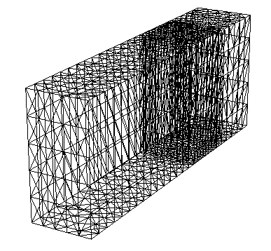
Figure 9: Poiseuille test – The domain and the mesh. Number of vertices: 1830. Number of elements (tetrahedra): 7830. Total number of variables: 12810.

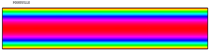
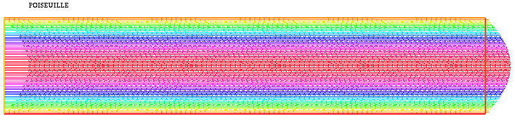
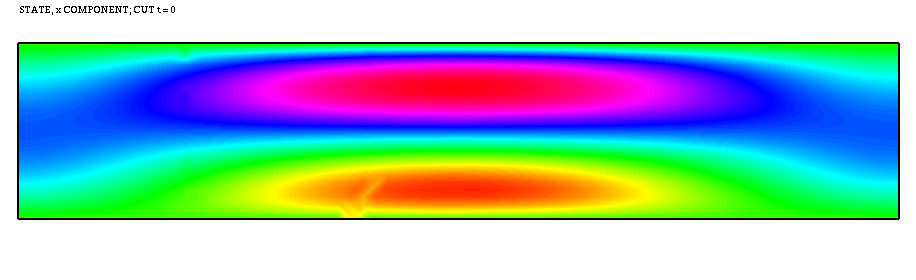
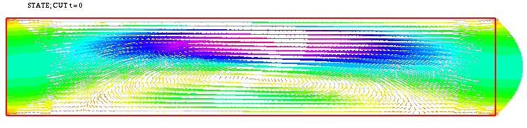
Figure 10: Poiseuille test – the target (Left) and the initial state (Right).

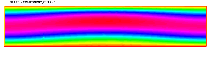
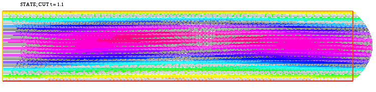
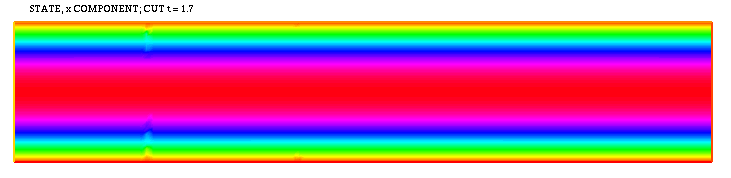
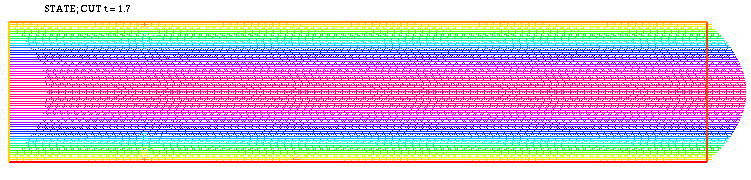
Figure 11: Poiseuille test – The state at $T=1.1$ (Left) and the state at $T=1.7$ ((Right).

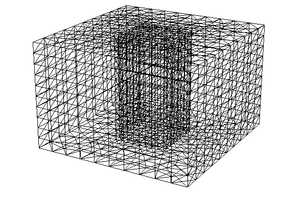
Figure 12: Taylor-Green test – The domain and the mesh. Number of vertices: 3146. Number of elements (tetrahedra): 15900. Total number of variables: 22022.

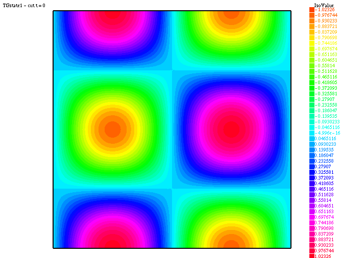
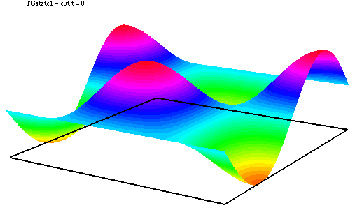
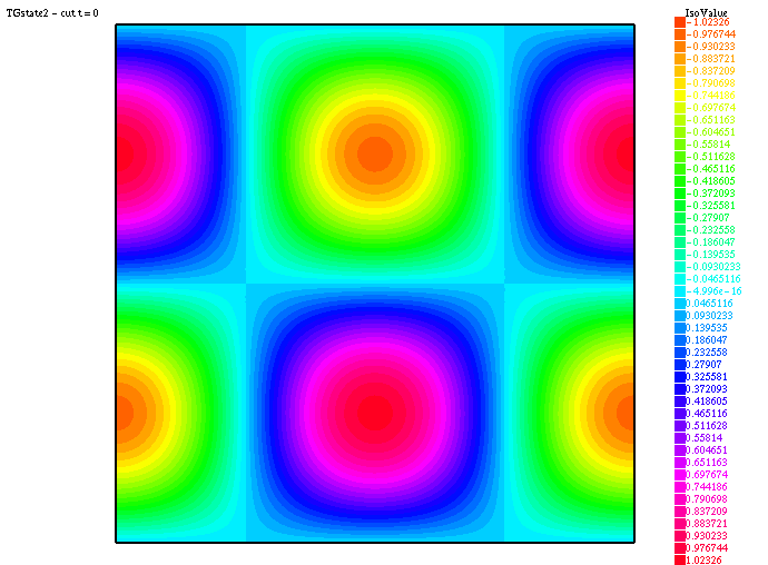
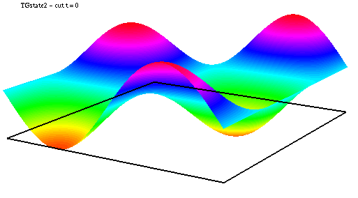
Figure 13: Taylor-Green test – First component of the initial datum (Left) and second component of the initial datum (Right).

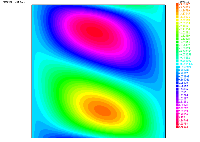
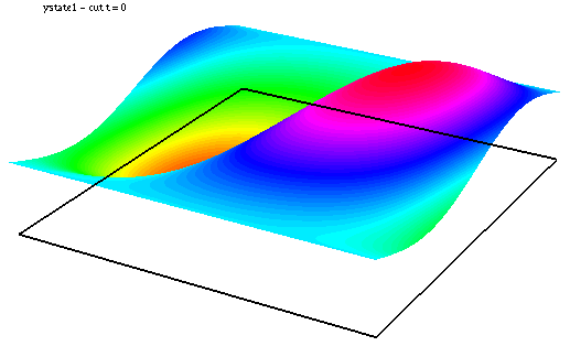
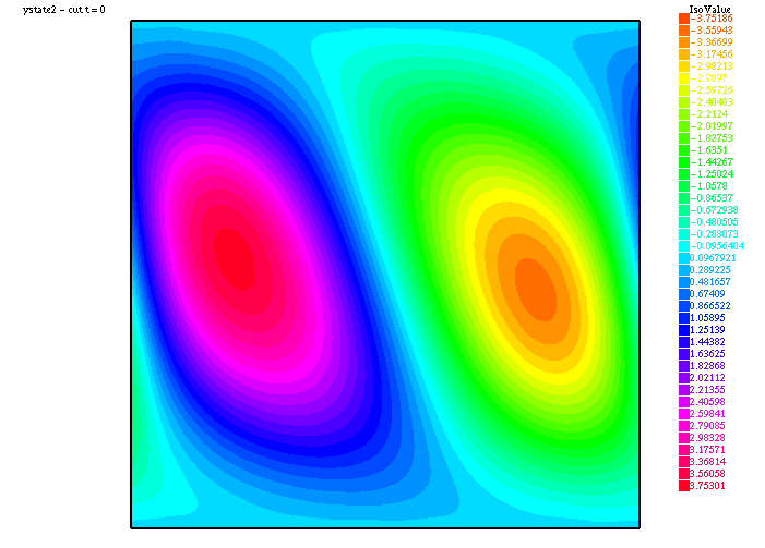
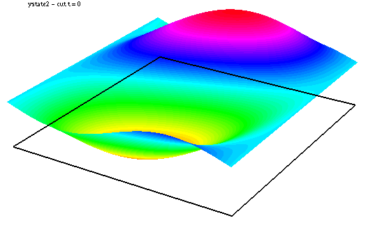
Figure 14: Taylor-Green test – The initial data: first component (Left) and second component (Right).

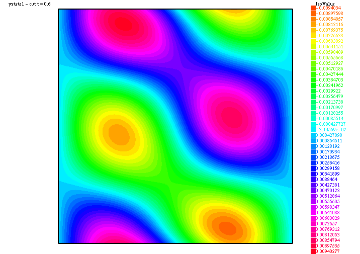
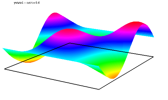
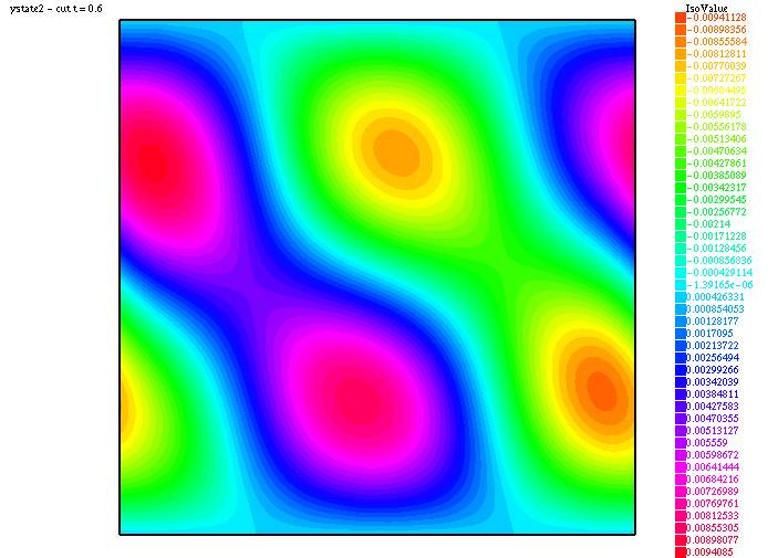
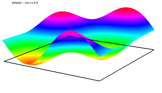
Figure 15: Taylor-Green test – The first component of the state (Left) and the second component of the state at $T=0.6$ ((Right).

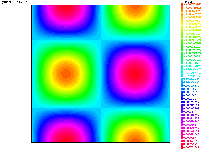
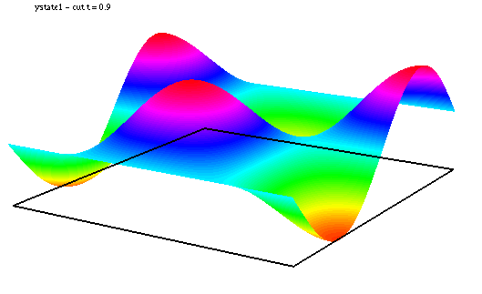
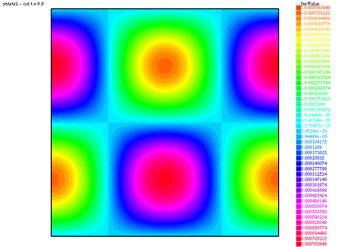
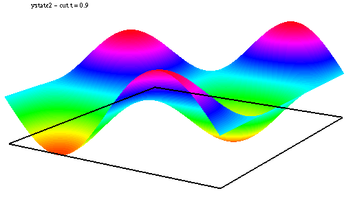
Figure 16: Taylor-Green test – The first component of the state (Left) and the second component of the state at $T=0.9$ ((Right).

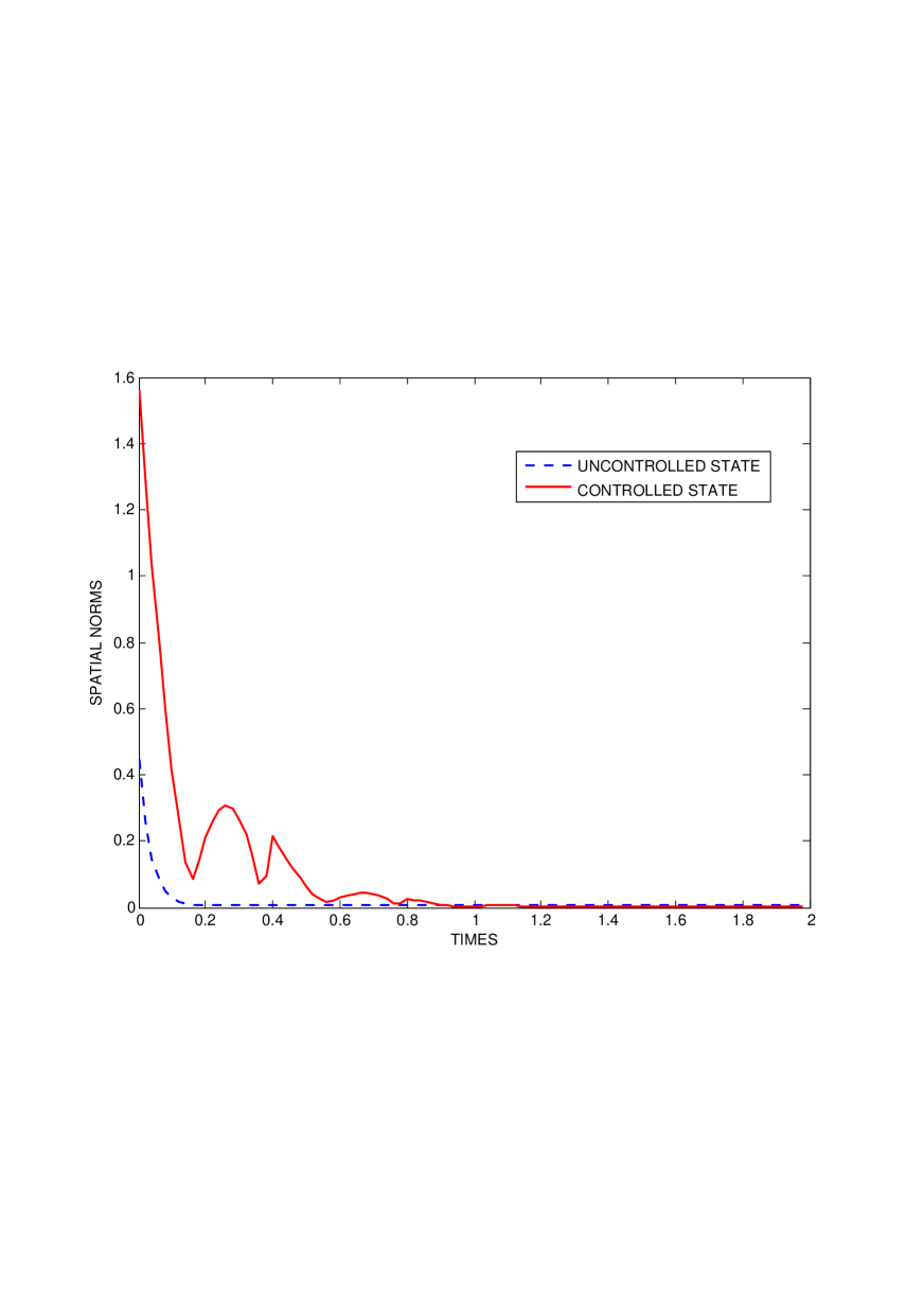
Figure 17: Poiseuille test – The $L^{2}$-norms of the deviations $\mathbf{y}-\overline{\mathbf{y}}_{P}$ and $\mathbf{z}-\overline{\mathbf{y}}_{P}$ corresponding to the computed controlled and uncontrolled states (Left) and a detail ((Right). Here, $T=2$. For instance, at $t=1.98$ we have $\|\mathbf{y}(\cdot\,,t)-\overline{\mathbf{y}}_{P}\|_{\mathbf{L}^{2}(\Omega)}=1.45367\cdot 10^{-7}$ and $\|\mathbf{z}(\cdot\,,t)-\overline{\mathbf{y}}_{P}\|_{\mathbf{L}^{2}(\Omega)}=0.00597072$.

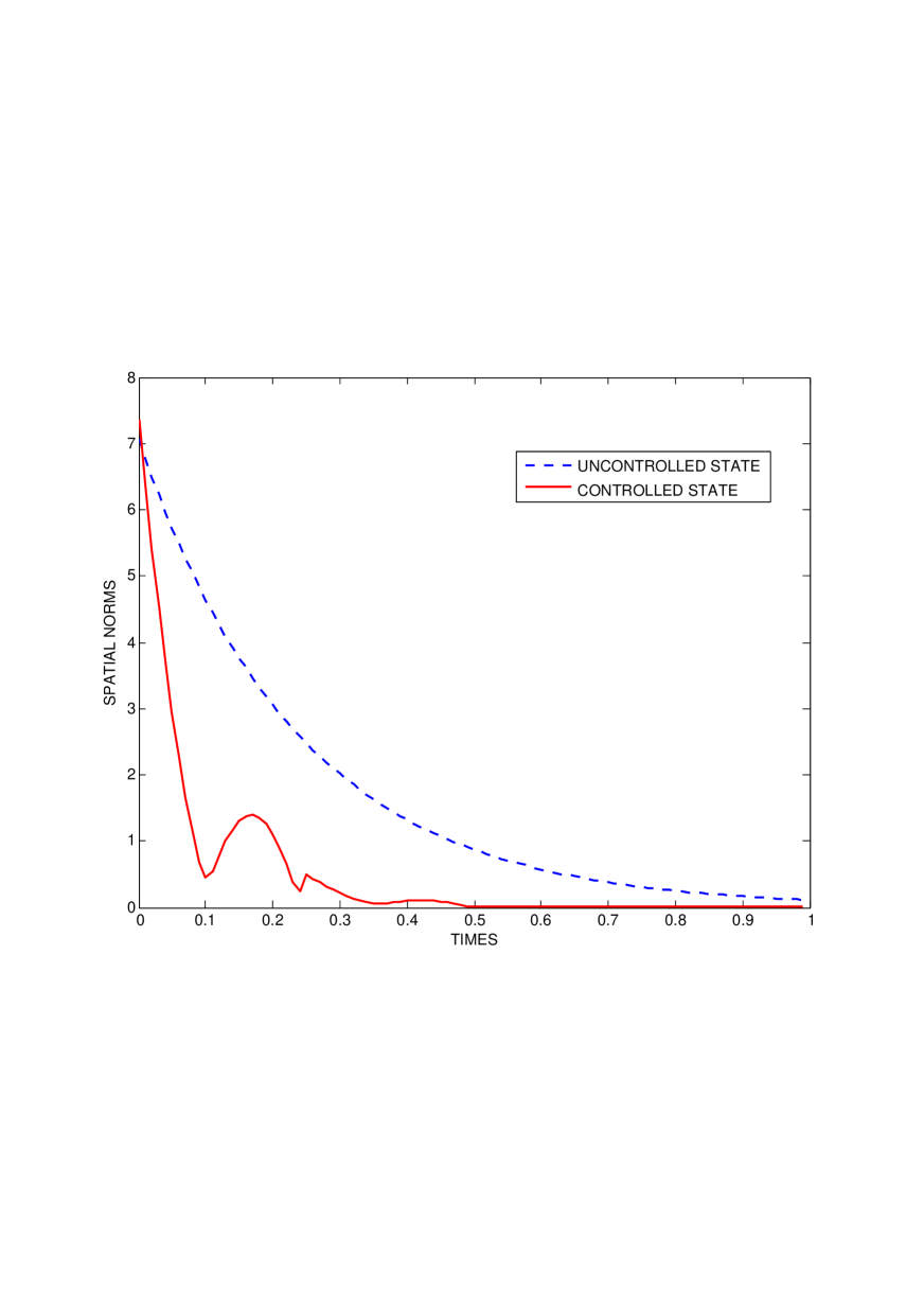
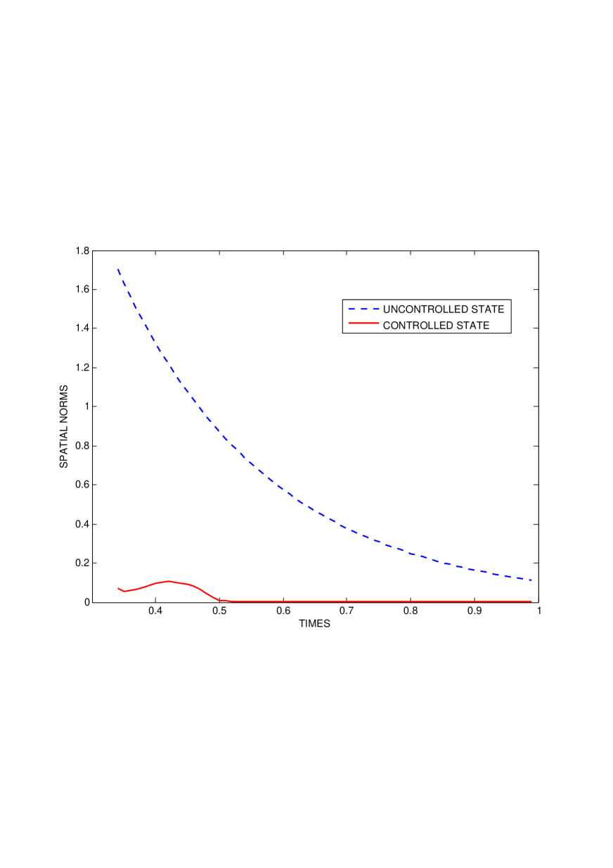
Figure 18: Taylor-Green test – The $L^{2}$-norms of the deviations $\mathbf{y}-\overline{\mathbf{y}}_{TG}$ and $\mathbf{z}-\overline{\mathbf{y}}_{TG}$ corresponding to the computed controlled and uncontrolled states (Left) and a detail ((Right). Here, $T=1$. For instance, at $t=0.99$ we have $\|\mathbf{y}(\cdot\,,t)-\overline{\mathbf{y}}_{TG}(\cdot\,,t)\|_{\mathbf{L}^{2}(\Omega)}=3.74645\cdot 10^{-10}$ and $\|\mathbf{z}(\cdot\,,t)-\overline{\mathbf{y}}_{TG}(\cdot\,,t)\|_{\mathbf{L}^{2}(\Omega)}=0.112909$.

5 Additional comments and conclusions

In this paper, we have seen that it is possible to solve numerically null controllability problems for the two-dimensional heat, Stokes and Navier-Stokes equations with Dirichlet boundary conditions. We have used some ideas that come from the so called Fursikov-Imanuvilov formulation and lead to the solution of high order partial differential problems in the space and time variables. The similar and simpler one-dimensional case was studied in [11].

There are two different ways to define numerical approximations of the resulting systems:

• By working with spatially $C^{1}$ finite element spaces or

• By introducing multipliers and working on (usual) $C^{0}$ finite element spaces.

In this paper, we have chosen the second approach. In a forthcoming paper, we will be concerned with the first one.

Unfortunately, in our case, the numerical approximation is not completely justified from a rigorous mathematical viewpoint. However, we have seen that the approximate problems can be solved in a relatively easy way and produce good numerical results.

Of course, the same ideas and techniques can be applied in many other similar situations: semilinear heat equations with (for instance) globally Lipschitz-continuous nonlinearities, Boussinesq-like systems, non-cylindrical control domains, boundary control problems, etc. Some results have been presented in [7, 10]; see also [12].

References

[1]F. Boyer, On the penalised HUM approach and its applications to
the numerical approximation of null-controls for parabolic problems, in
CANUM 2012, Super-Besse, ESAIM Proc., EDP Sci., Les Ulis, 2013.
[2]F. Boyer, F. Hubert, and J. Le Rousseau, Uniform controllability
properties for space/time-discretized parabolic equations, Numer. Math., 118
(2011), pp. 601–661.
[3]F. Brezzi and M. Fortin, Mixed and hybrid finite element methods,
vol. 15 of Springer Series in Computational Mathematics, Springer-Verlag, New
York, 1991.
[4]C. Carthel, R. Glowinski and J.-L. Lions, On exact and approximate
boundary controllability for the heat equation: a numerical approach,
J. Optimization, Theory and Applications 82(3), (1994) 429–484.
[5]P. G. Ciarlet, The finite element method for elliptic problems,
vol. 40 of Classics in Applied Mathematics, Society for Industrial and
Applied Mathematics (SIAM), Philadelphia, PA, 2002.
Reprint of the 1978 original [North-Holland, Amsterdam; MR0520174 (58
#25001)].
[6]P. G. Ciarlet and J. L. Lions, eds., Handbook of numerical analysis.
Vol. IX, Handbook of Numerical Analysis, IX, North-Holland, Amsterdam,
2003.
Numerical methods for fluids. Part 3.
[7]N. Cîndea, E. Fernández-Cara, and A. Münch, Numerical
controllability of the wave equation through primal methods and Carleman
estimates, ESAIM Control Optim. Calc. Var., 19 (2013), pp. 1076–1108.
[8]S. Ervedoza and J. Valein, On the observability of abstract time-discrete
linear parabolic equations, Rev. Mat. Complut., 23 (2010), no. 1, 163–190.
[9]E. Fernández-Cara, S. Guerrero, O. Y. Imanuvilov, and J.-P. Puel,
Local exact controllability of the Navier-Stokes system, J. Math.
Pures Appl. (9), 83 (2004), pp. 1501–1542.
[10]E. Fernández-Cara and A. Münch, Numerical null
controllability of semi-linear 1-D heat equations: fixed point, least
squares and Newton methods, Math. Control Relat. Fields, 2 (2012),
pp. 217–246.
[11]E. Fernández-Cara and A. Münch, Strong convergence
approximations of null controls for the 1D heat equation, SMA
J., 61 (2013), pp. 49–78.
[12]E. Fernández-Cara and A. Münch, Numerical exact
controllability of the 1D heat equation: duality and Carleman weights,
J. Optim. Theory Appl., 163 (2014), pp. 253–285.
[13]A. V. Fursikov and O. Y. Imanuvilov, Controllability of evolution
equations, vol. 34 of Lecture Notes Series, Seoul National University
Research Institute of Mathematics Global Analysis Research Center, Seoul,
1996.
[14]R. Glowinski, Finite element methods for incompressible viscous
flow, in Handbook of numerical analysis, Vol. IX, Handb. Numer. Anal.,
IX, North-Holland, Amsterdam, 2003, pp. 3–1176.
[15]M. González-Burgos, S. Guerrero, and J.-P. Puel, Local exact
controllability to the trajectories of the Boussinesq system via a
fictitious control on the divergence equation, Commun. Pure Appl. Anal., 8
(2009), pp. 311–333.
[16]M. D. Gunzburger, Perspectives in flow control and optimization,
vol. 5 of Advances in Design and Control, Society for Industrial and Applied
Mathematics (SIAM), Philadelphia, PA, 2003.
[17]F. Hecht, New development in freefem++, J. Numer. Math., 20 (2012),
pp. 251–265.
[18]O. Y. Imanuvilov, Remarks on exact controllability for the
Navier-Stokes equations, ESAIM Control Optim. Calc. Var., 6 (2001),
pp. 39–72 (electronic).
[19]O. Y. Imanuvilov, J.-P. Puel, and M. Yamamoto, Carleman estimates
for second order non homogeneous parabolic equation, to appear.
[20]S. Labbé and E. Trélat, Uniform controllability of semi-discrete
approximations of parabolic control systems, Systems and Control Letters 55
(2006), 597–609.
[21]A. Münch and D. A. Souza, A mixed formulation for the direct
approximation of -weighted controls for the linear heat equation, To
appear in Adv. Comput. Math. (http://hal.archives-ouvertes.fr/hal-00998765).
[22]W. Queck, The convergence factor of preconditioned algorithms of the
Arrow-Hurwicz type, SIAM J. Numer. Anal., 26 (1989), pp. 1016–1030.
[23]J.-P. Raymond, Stokes and Navier-Stokes equations with a
nonhomogeneous divergence condition, Discrete Contin. Dyn. Syst. Ser. B, 14
(2010), pp. 1537–1564.
[24]J. E. Roberts and J.-M. Thomas, Mixed and hybrid methods, in
Handbook of numerical analysis, Vol. II, Handb. Numer. Anal., II,
North-Holland, Amsterdam, 1991, pp. 523–639.