Self-consistent context aware conformer transducer for speech recognition

Abstract

We propose a novel neural network architecture based on conformer transducer that adds contextual information flow to the ASR systems. Our method improves the accuracy of recognizing uncommon words while not harming the word error rate of regular words. We explore the uncommon words accuracy improvement when we use the new model and/or shallow fusion with context language model. We found that combination of both provides cumulative gain in uncommon words recognition accuracy.

Index Terms: speech recognition, sequence-to-sequence, neural networks, speech hints, context aware model.

1 Introduction

End-to-end speech-to-text systems became major technology in voice recognition due to their superior performance over previously widely used multi-component HMM-DNN systems. Among variety of model architectures we can highlight the following: Connectionist Temporal Classification [1], Listen-Attend-Spell [2], Time-Depth Separable Convolutions [3], Recurrent Neural Network Transducer [4], Transformer [5], Conformer [6], SqueezeFormer [7], Fast Conformer[8], Zipformer [9]. All these architectures are encoder-decoder models. One of the major limitations of an E2E system is inability to accurately recognize words that either never appeared or rarely appeared in training data, for example, entity names, person names etc. To address this issue the model based approach and decoding based approach were suggested. The first one implies the modification of the model to incorporate user provided context words [10], [11], [10], while the second one addresses the challenge by applying external context score though shallow fusion or on-the-fly re-scoring [12], [13].

2 Model

2.1 Conformer transducer

We consider a set of audio features $X$ as an input and an utterance of tokens $Y$ as an output of the model. The sequence-to-sequence model encodes $X$ in to hidden vector representation by passing input data to encoder and then uses decoder to predict output tokens. The transducer model consists of the three main modules: an audio encoder, a predictor (also mentioned in the publications as predictor network or decoder) and a joiner or joint network, see Fig.1. The audio encoder consists of stacked conformer layers [6]. We used modified predictor network [14] as predictor: we added convolution layer. The joint network combines the audio encoder outputs $h^{a}$ and predictor outputs $h^{d}$ and then the joiner outputs $z$ is fed the softmax layer. The result is a probability vector over blank symbol and output tokens. We use sentence piece tokenization [15].

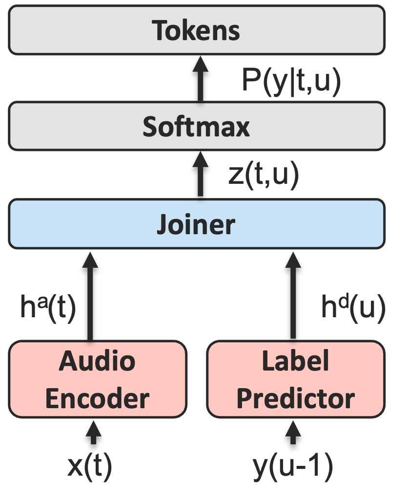
Fig. 1: Transducer architecture.

2.2 Context Conformer Transducer

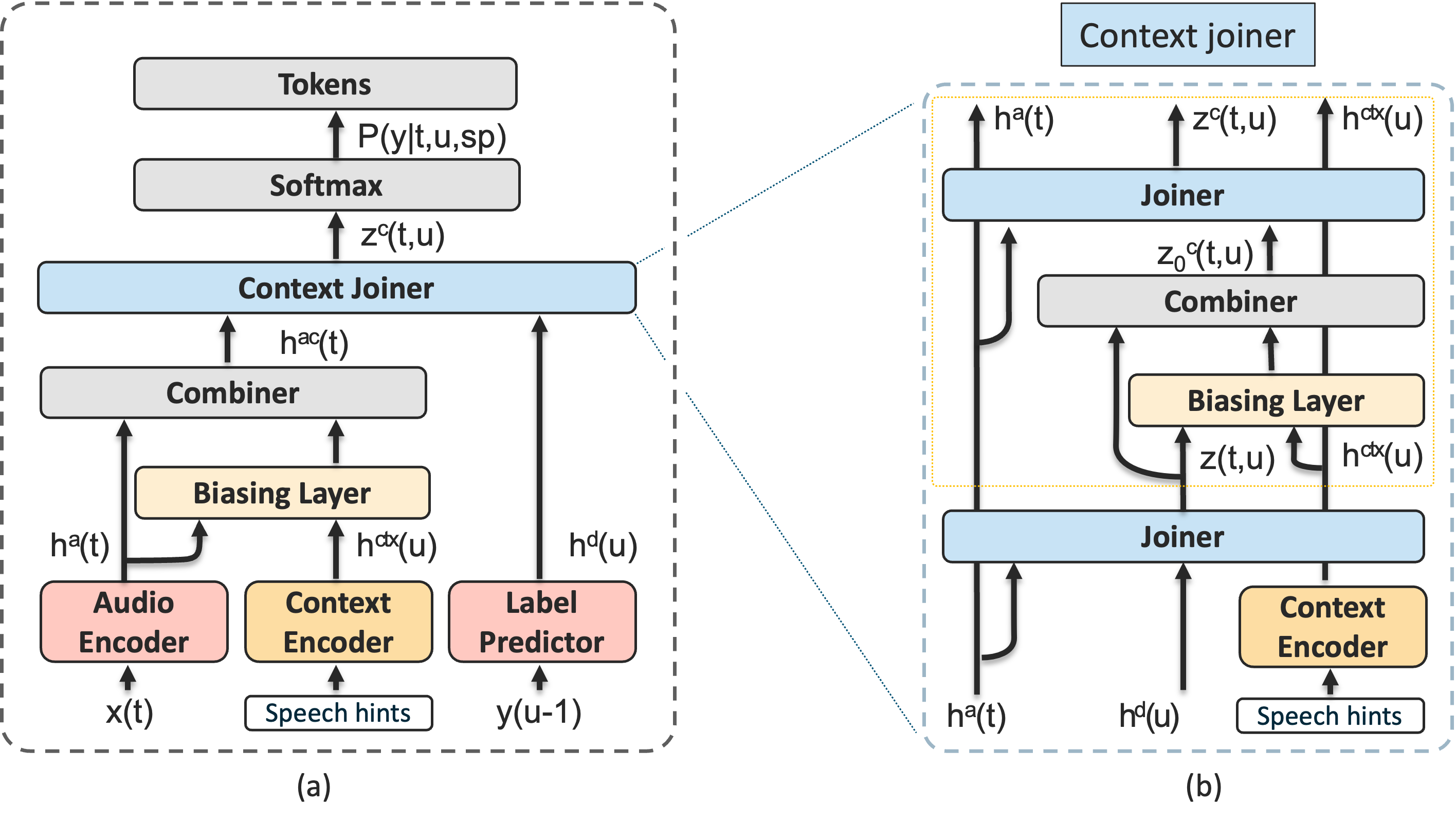
Fig. 2: Context Transducer architecture.

Audio Encoder: To add context information to ASR model we add several modules. We follow the architecture of Context-Aware Transducer Transformer proposed in [11]. The additional modules are context encoders, biasing layers and combiners, see Fig.2. We add them to the output of audio encoder and joiner.

The context encoder is fed by personal information such as user names, company names or any other user provided words and phrases - speech hints. The context encoder consists of embedding layer and stacked BLSTM layers. First, the list of user speech hints is tokenized into a sequence of tokens, then it is fed into embedding layer and following BLSTM layers. The last hidden state of BLSTM is used as embedded vector representation of the speech hints. The output of the corresponding context encoder is mixed with the outputs of audio encoder and joiner. We use the identical context encoder modules to do this, but the exact methods of mixing are different.

First, let’s consider the audio encoder. The outputs of the audio encoder and context encoder are fed to the biasing layer. The latest is a multihead attention layer whose queries $Q$ are audio encoder outputs, keys $K$ and values $V$ are context encoder outputs which are embedded vector representation of the speech hints. The attention is computed by the following expression:

$$HW^{ca}=Softmax\left(\frac{Q^{ca}K^{ca}}{\sqrt{d}}\right)V^{ca}$$ (1)

The resulted scores from softmax layer are used to add weighted contribution from speech hints embeddings resulting in $HW^{ca}$. This value is fed to combiner layer that consists of two normalization layers, concatenation and following linear projection layer:

$$\begin{array}[]{@{}l@{}}H^{cat}=concat\left(LayerNorm(h^{a}),LayerNorm(HW^{ca})\right)\\ H^{ca}=Linear(H^{cat})\end{array}$$ (2)

Label Predictor: The next obvious step would be adding context encoder modules to label predictor. We skipped this step for the following reasons. The label predictor acts like an internal language model: having a sequence of previously generated token $y[u-m,...,u-1]$ the label predictor generate a hidden vector. If we add a softmax layer on top of it, we will get an architecture of the language model. If such a neural net has enough learnable parameters and proper architecture, it can predict the next token or word. In our case we have very simple label predictor consisting of embedding vector and convolution layer. It is hard to expect a good quality of the next token prediction in this case. If we try to add context encoder modules to our label predictor, we will get the following: having previously generated tokens and the label predictor we are trying to predict what speech hint from the list to attend. If the predictor is poor in quality the result of attending is poor in quality as well. This is supported by our experiments.

Context Joiner: We found that context encoder with label predictor does not work because we can’t properly attend speech hints embeddings. What if we take the output of the joiner instead of label predictor? The output of the joiner is a hidden representation of all previously generated tokens for the current timestamp $t$ and we can use it to attend speech hints and find with a good confidence what speech hint is currently the most important. Then we can combine the attention result with joiner output and use it again as joiner input instead of label predictor output.

Let’s write this into equations:

$$\left\{\begin{array}[]{@{}l@{}}z_{t,u}=Joiner(h^{a}_{t},z_{t,u,c})\\ z_{t,u,c}=Combiner(z_{t,u},h^{c}),\end{array}\right.\$$ (3)

where $z_{t,u,c}$ is $h^{d}_{u}$ at the very beginning. We got a self-recurrent equation.

To solve the mentioned above problem, we used self-consistent approach that is widely used in semiconductor physics. Let’s us briefly describe it. One of the core tasks in applied semiconductor physics is to solve Schrödinger equation together with Poisson equation:

$$\left\{\begin{array}[]{@{}l@{}}-\dfrac{\partial^{2}F(x)}{\partial x^{2}}+V(x)F(x)=EF(x)\\ \dfrac{\partial^{2}V(x)}{\partial x^{2}}=\left|F(x)\right|^{2}\end{array}\right.\,$$ (4)

Where $E$ is energy, $F$ is wavefunction and $V$ is band profile. We omitted physical constants like electron charge for simplicity. We need to find $F$ and $V$. We can’t solve these equations directly altogether but we can solve them iteratively. First, we assume $V(x)\equiv 0$ and solve the first equation. Having $F(x)$ we can solve the second equation and get $V(x)$. Then we can return to the first equation with a new $V(x)$, solve it and get $F(x)$. We repeat this procedure until both $V(x)$ and $F(x)$ converge to their asymptotes, when the differences of functions between iteration become below a predefined threshold. The method is called self-consistent calculations and we are going to apply it to our task.

We can apply this technique to solve the equations (3). First, we take $h^{a}_{t}$ and $h^{d}_{u}$ as inputs and compute the joiner output $z_{t,u}$. Then we compute the combiner output $z_{t,u,c}$ and feed it to the joiner again. We repeat this process until the joiner output from iteration $n$ differs from joiner output from iteration $n-1$ by some small value. In practice, the converge is good and three iterations is enough, see Table 1. The second column shows an averaged maximum difference between joiner output from iteration $n$ and iteration $n-1$, the third - averaged mean difference.

Table 1: Convergence of self-consistent iterations

Iteration number	Avg max diff	Avg mean diff
1	3852403.100	1.35E-02
2	24.31	-3.99E-08
3	0.21	-8.99E-12
4	0.02	-7.55E-13
5	0.01	1.29E-12

The detailed roll out diagram of the data flow when $n$ is equal to 1 is shown in Fig.2(b). For $n>1$ we need to repeat modules in orange dotted block.

3 Experimental setup

We use about 12K hours of speech audio from in-house dataset to train the model and 40 hours to evaluate it. The datasets are consisted of the audio collected from Webex Meetings. We use synthetic speech hints that are generated on-the-fly to train our model. The process of generation is the following:

$\bullet$

We randomly peek a set of words from the ground truth text. Then we randomly augment each of the word by doubling one or more characters. For example, cat becomes catt, triple becomes tripple etc.

$\bullet$

We randomly augment the selected speech hints words in a way to get similar sounding words. For example, we swap k $\Leftrightarrow$ c, j $\Leftrightarrow$ g etc. Some words change only one letter, some more: cat $\Rightarrow$ kat, ginger $\Rightarrow$ jinger, cereal $\Rightarrow$ serial, hay $\Rightarrow$ hey

$\bullet$

We create three types of samples:

$\bullet$

Original samples. Data that covers the case when no speech hints are provided.

$\bullet$

Samples with only negative speech hints. This covers the case when none of speech hints are encountered in the ground truth.

$\bullet$

Samples with positive and negative speech hints. This covers the case when some of the speech hints are in the ground truth.

The model consists of 12 causal conformer layers with hidden dimensions of 256 and feedforward dimension of 2048. The context encoder is a two layer BLSTM with dimension of 256. Overall number of trainable parameters in our model is about 85.2M. We train the model with pruned transducer loss function [16]. We used K2 icefall package [17] to train the model.

4 Results and discussion

To evaluate the results of experiments we used relative word error rate (WERR) and out-of-vocabulary words accuracy recognition (OOV Accuracy). The WERR is computed as relative change in WER in the experiment with speech hints in comparison with a case where no speech hints are provided. The OOV accuracy is computed as a number of correctly transcribed speech hints in the utterance divided to the total number of speech hints in the utterance.

The speech hints for test dataset were created the following way. We filtered the words from the test dataset that are not encountered in the train dataset. Then we take words that appears only once in test set. We vary the total number of speech hints in the evaluation from 100 to 1000.

Table 2: WERR and OOV accuracy with different ways of providing speech hints

Model configuration	Number of speech hints	WERR, %	OOV Accuracy, %
No hints	0	0	8.3
Context encoder	100	0.76	12.03
Shallow fusion	100	-1.33	33.08
Context encoder + Shallow fusion	100	-2.32	45.11
Context encoder	200	0.95	10.68
Shallow fusion	200	-2.39	36.89
Context encoder + Shallow fusion	200	-0.08	41.42
Context encoder	500	3.50	14.19
Shallow fusion	500	-3.99	35.33
Context encoder + Shallow fusion	500	0.46	36.8
Context encoder	1000	3.00	14.52
Shallow fusion	1000	-4.37	35.01
Context encoder + Shallow fusion	1000	-1.41	35.21

The results of experiments are shown in Table 2. The first row show the results of the baseline experiment when no speech hints are provided (WERR is zero). The second row is the experiment when we feed speech hints to the context encoders of the model. The third row is the experiment when speech hints are used only in shallow fusion. The fourth row is the experiment when both techniques are used. We provide the results for the 100, 200, 500 and 1000 number of speech hints. As we can see from the table, applying context encoder processing of the speech hints gets about 50% of OOV accuracy improvement, when the number of speech hints is 100. Using of shallow fusion provides even better improvement, from 8.3% to 33%. The use of both context encoders and shallow gets OOV accuracy increase by nearly 4.5 times. At the same time WER change does not exceed 2.3% across all experiments. Similar behavior can be observed for the larger number of speech hints. The results of experiments show that using context encoder architecture together with shallow fusion provides significant improvement in OOV accuracy while keeping WER without noticeable change.

5 Conclusion

We proposed a novel architecture of the transducer-based automatic speech recognition model that includes the contextual data.

We have shown that using this architecture together with context language model shallow fusion leads to cumulative improvement of uncommon words recognition.

The proposed architecture does not depend on particular encoder implementation and can be applied to the recently proposed encoders such as SqueezeFormer [7], Fast Conformer[8] and Zipformer [9].

References

- [1] A. Graves, S. Fernandez, F. Gomez, and J. Schmidhuber. Connectionist temporal classification: Labelling unsegmented sequence data with recurrent neural nets. In ICML ’06: Proceedings of the International Conference on Machine Learning, 2006.
- [2] William Chan, Navdeep Jaitly, Quoc V. Le, and Oriol Vinyals. Listen, attend and spell: A neural network for large vocabulary conversational speech recognition. In ICASSP, 2016.
- [3] Awni Hannun, Ann Lee, Qiantong Xu, and Ronan Collobert. Sequence-to-sequence speech recognition with time-depth separable convolutions, 2019.
- [4] A. Graves. Sequence Transduction With Recurrent Neural Networks. ArXiv e-prints, November 2012.
- [5] Linhao Dong, Shuang Xu, and Bo Xu. Speech-transformer: A no-recurrence sequence-to-sequence model for speech recognition. In 2018 IEEE International Conference on Acoustics, Speech and Signal Processing (ICASSP), pages 5884–5888, 2018.
- [6] Anmol Gulati, James Qin, Chung-Cheng Chiu, Niki Parmar, Yu Zhang, Jiahui Yu, Wei Han, Shibo Wang, Zhengdong Zhang, Yonghui Wu, and Ruoming Pang. Conformer: Convolution-augmented transformer for speech recognition, 2020.
- [7] Sehoon Kim, Amir Gholami, Albert Shaw, Nicholas Lee, Karttikeya Mangalam, Jitendra Malik, Michael W. Mahoney, and Kurt Keutzer. Squeezeformer: An efficient transformer for automatic speech recognition, 2022.
- [8] Dima Rekesh, Nithin Rao Koluguri, Samuel Kriman, Somshubra Majumdar, Vahid Noroozi, He Huang, Oleksii Hrinchuk, Krishna Puvvada, Ankur Kumar, Jagadeesh Balam, and Boris Ginsburg. Fast conformer with linearly scalable attention for efficient speech recognition, 2023.
- [9] Zengwei Yao, Liyong Guo, Xiaoyu Yang, Wei Kang, Fangjun Kuang, Yifan Yang, Zengrui Jin, Long Lin, and Daniel Povey. Zipformer: A faster and better encoder for automatic speech recognition, 2023.
- [10] Kanthashree Mysore Sathyendra, Thejaswi Muniyappa, Feng-Ju Chang, Jing Liu, Jinru Su, Grant P. Strimel, Athanasios Mouchtaris, and Siegfried Kunzmann. Contextual adapters for personalized speech recognition in neural transducers, 2022.
- [11] Feng-Ju Chang, Jing Liu, Martin H. Radfar, Athanasios Mouchtaris, Maurizio Omologo, Ariya Rastrow, and Siegfried Kunzmann. Context-aware transformer transducer for speech recognition. 2021 IEEE Automatic Speech Recognition and Understanding Workshop (ASRU), pages 503–510, 2021.
- [12] Ding Zhao, Tara N. Sainath, David Rybach, Pat Rondon, Deepti Bhatia, Bo Li, and Ruoming Pang. Shallow-Fusion End-to-End Contextual Biasing. In Proc. Interspeech 2019, pages 1418–1422, 2019.
- [13] Weiran Wang, Zelin Wu, Diamantino Caseiro, Tsendsuren Munkhdalai, Khe Chai Sim, Pat Rondon, Golan Pundak, Gan Song, Rohit Prabhavalkar, Zhong Meng, Ding Zhao, Tara Sainath, and Pedro Moreno Mengibar. Contextual biasing with the knuth-morris-pratt matching algorithm, 2023.
- [14] Mohammadreza Ghodsi, Xiaofeng Liu, James Apfel, Rodrigo Cabrera, and Eugene Weinstein. Rnn-transducer with stateless prediction network. In ICASSP 2020 - 2020 IEEE International Conference on Acoustics, Speech and Signal Processing (ICASSP), pages 7049–7053, 2020.
- [15] Taku Kudo and John Richardson. Sentencepiece: A simple and language independent subword tokenizer and detokenizer for neural text processing, 2018.
- [16] Fangjun Kuang, Liyong Guo, Wei Kang, Long Lin, Mingshuang Luo, Zengwei Yao, and Daniel Povey. Pruned rnn-t for fast, memory-efficient asr training. In Proc. Interspeech 2022, pages 2068–2072, 2022.
- [17] K2 icefall. https://github.com/k2-fsa/icefall, 2023.