Modular Redesign of Mechatronic Systems: Formulation of Module Specifications Guaranteeing System Dynamics Specifications

Abstract

Complex mechatronic systems are typically composed of interconnected modules, often developed by independent teams. This development process challenges the verification of system specifications before all modules are integrated. To address this challenge, a modular redesign framework is proposed in this paper. Herein, first, allowed changes in the dynamics (represented by frequency response functions (FRFs)) of the redesigned system are defined with respect to the original system model, which already satisfies system specifications. Second, these allowed changes in the overall system dynamics (or system redesign specifications) are automatically translated to dynamics (FRF) specifications on module level that, when satisfied, guarantee overall system dynamics (FRF) specifications. This modularity in specification management supports local analysis and verification of module design changes, enabling design teams to work in parallel without the need to iteratively rebuild the system model to check fulfilment of system FRF specifications. A modular redesign process results that shortens time-to-market and decreases redesign costs. The framework’s effectiveness is demonstrated through three examples of increasing complexity, highlighting its potential to enable modular mechatronic system (re)design.

1 Introduction

Most complex mechatronic systems consist of multiple interconnected modules/components. These systems need to satisfy given design specifications related to their dynamic behaviour on the level of the overall system. However, in many cases, the modules are developed and designed by independent teams of specialized engineers, which introduces a challenge related to the complexity of the design process. Namely, if specifications are only provided on a system level, the satisfaction of these specifications can only be verified after all modules have been designed and integrated (or interconnected), see Figure 1. This may lead to unexpected behavior which could necessitate the need for (expensive) redesigns. In addition, this leads to a design cycle where delays are unavoidable, as each module design needs to be completed before verification can take place [nielsen2015systems].

Figure 1: Integrated design procedure.

Therefore, the aim is often to achieve a modular design approach that decouples the design cycles of modules [baldwin2000design]. A modular design approach for mechatronic systems requires the formulation of module specifications, given the overall system dynamics specifications [zheng2017multidisciplinary, van2010modular, hamraz2012multidomain]. Then, when the modules are designed, the satisfaction of their respective specifications can be verified on a module level. In theory, if all modules are finished and satisfy their specifications, the complete system can directly be integrated and is guaranteed to satisfy system-level specifications (see Figure 2).

Figure 2: Modular design procedure.

Such a modular design approach allows for example parallel design threads of engineering teams, easier replacement of modules of the system and modularity in complexity reduction [giese2004modular, habib2014comparative, barbieri2014model, zheng2019interface]. However, many challenges persist when aiming to develop a modular design approach. First, the modules and the interfaces between them need to be clearly defined. Second, a framework to efficiently determine module specifications based on the overall system specifications is required. These module specifications need to be feasible and realistic. Third, if all components satisfy their respective specifications, the satisfaction of the overall system specifications needs to be guaranteed. Finally, the approach has to be scalable to complex systems with multiple modules with complex interactions.

In general, all of these challenge make “first time right” design often infeasible in practice. In addition, system specifications could change during (or even after) the design process which could require updates in the design. Therefore, the need arises for a modular redesign approach in which existing designs are already available but one or more components of the system need to be replaced/changed. Such an approach is also called continuous, evolutionary or incremental development [grimheden2013can, de2021process, maier1998architecting].

In a modular redesign procedure, system-level specifications need to be translated to module-level specifications such that proposed updated module designs can be verified without the need to test the updated system as a whole. In [janssen2023modular] and [janssen2022modular], a modular approach is introduced for another purpose, i.e., modular model complexity management.

In [janssen2022modeselect], this approach was introduced specifically for the complexity management of interconnected structural dynamics models. In these works, requirements on the accuracy of a desired reduced-order interconnected model are translated to accuracy requirements on reduced-order subsystem models. In turn, satisfaction of these FRF requirements for each subsystem guarantees the required accuracy of the reduced-order interconnected system model. Specifically, requirements are given as bounds on the maximum allowed changes in the frequency response functions (FRFs). Such bounds are also used in control systems to guarantee for example the stability or performance of a system in the presence of uncertainties, see e.g., [iwasaki2005time, iwasaki2007feedback] or [nordebo1999semi]. As such, methods from the field of robust control [zhou1998essentials] have been proven useful to support modular model complexity management.

The main contribution of this work is to show how this line of reasoning can also be exploited to develop a novel, fully modular redesign framework which guarantees the satisfaction of specifications on the system-level input-output behavior, described by a FRF. This is achieved by first introducing a general modular modelling framework in which FRF representations of the modules’ dynamics are interconnected to obtain the overall system dynamics (in terms of FRFs). In addition, frequency-based system-level specifications are introduced, which define how much the dynamics of the interconnected system are allowed to change in the frequency domain. With these specifications at hand, we show that module specifications of a similar nature can be automatically computed that, when satisfied, guarantee satisfaction of the overall system specifications. These module specifications enable a modular redesign process where proposed design changes in the modules can be analysed and verified locally (i.e., on module level), which enables a work-flow in which design teams can work fully in parallel. This may significantly reduce time-to-market and decrease redesign costs.

The proposed redesign framework is demonstrated on three mechatronic use cases of increasing complexity: 1) an illustrative academic example in the form of a two-mass-spring-damper system, 2) a six component pillar-and-plate benchmark model and 3) the model of an industrial wire bonder used in the semi-conductor industry.

The remainder of this paper is organized as follows. Section 2 introduces the modular modelling framework. In Section 3, a way to represent redesign specifications in the frequency domain using FRFs is introduced. In Section 4, the main contribution of this paper will be discussed: How to translate system FRF specifications to module FRF specifications that guarantee the required system-level dynamic behaviour. We will illustrate this approach on three different use case systems in Section LABEL:sec:examples and close with conclusions in Section LABEL:sec:conclusion.

2 General framework for modular modelling

To enable model-based modular redesign of systems, we will introduce a general modelling framework that can be used to model interconnected systems. Here, we focus on the dynamic behaviour of such systems having linear dynamics and model the system as a set of interconnected FRFs.

In this framework, we assume that each of the $k$ original modules can be modelled as a multiple-input multiple-output (MIMO) FRF given by

$$y^{(j)}(i\omega)=G^{(j)}(i\omega)u^{(j)}(i\omega)$$ (1)

for $j=1,2,\dots,k$ and where $\omega\in\mathbb{R}$ represents frequency. Modular redesign would generally lead to a change in FRF, which is represented as

$$\hat{y}^{(j)}(i\omega)=\hat{G}^{(j)}(i\omega)\hat{u}^{(j)}(i\omega)$$ (2)

for $j=1,2,\dots,k$ for all $\omega\in\mathbb{R}$. We assume that both the original and redesigned modules have the same number of $m_{j}$ inputs and $p_{j}$ outputs. Therefore, the complex matrix $G^{(j)}(i\omega)$ and $\hat{G}^{(j)}(i\omega)$ have the same dimensions ($p_{j}\times m_{j}$).

To enable a systematic approach for connecting the modules, the $k$ module FRFs are collected in a block diagonal FRF,

$$G_{B}(i\omega) =\textrm{diag}\big{(}G^{(1)}(i\omega),\dots,G^{(k)}(i\omega)\big{)}$$ (3)

$$\hat{G}_{B}(i\omega) =\textrm{diag}\big{(}\hat{G}^{(1)}(i\omega),\dots,\hat{G}^{(k)}(i\omega)\big{)}$$ (4)

for the original modules and redesigned modules, respectively, for all $\omega\in\mathbb{R}$. Then, the interconnection between modules is modelled as signals from outputs of modules ($y_{B}:=[y^{{(1)}^{\top}},\dots,y^{{(k)}^{\top}}]^{\top}$ or $\hat{y}_{B}(i\omega):=[\hat{y}^{{(1)}^{\top}},\dots,\hat{y}^{{(k)}^{\top}}]^{\top}$) to inputs of (other) modules ($u_{B}(i\omega):=[u^{{(1)}^{\top}},\dots,u^{{(k)}^{\top}}]^{\top}$ or $\hat{u}_{B}(i\omega):=[\hat{u}^{{(1)}^{\top}},\dots,\hat{u}^{{(k)}^{\top}}]^{\top}$). This is captured in the interface matrix $\mathcal{K}_{BB}$, as is common with interconnected LTI systems in the field of control [sandberg2009model, reis2008survey]. Furthermore, we define the system’s $m_{A}$ external input signals by $u_{A}(i\omega)$ and its $p_{A}$ external output signals by $y_{A}(i\omega)$. These are connected to the modules via matrices $\mathcal{K}_{AB}$ and $\mathcal{K}_{BA}$, respectively. The complete interconnection structure $\mathcal{K}$ is then given by

$$\left[\begin{array}[]{c}u_{B}\\ y_{A}\end{array}\right] =\mathcal{K}\left[\begin{array}[]{c}y_{B}\\ u_{A}\end{array}\right]\text{ and }\left[\begin{array}[]{c}\hat{u}_{B}\\ \hat{y}_{A}\end{array}\right]=\mathcal{K}\left[\begin{array}[]{c}\hat{y}_{B}\\ u_{A}\end{array}\right]$$ (13)

$$\text{ with }\mathcal{K} =\left[\begin{array}[]{cc}\mathcal{K}_{BB}&\mathcal{K}_{BA}\\ \mathcal{K}_{AB}&0\end{array}\right].$$ (16)

Note that we assume here that the interconnection structure $\mathcal{K}$ is the same for the original and the redesigned modules. Using this modular modelling framework illustrated in Figure 3, we can define the system’s original FRF from $u_{A}$ to $y_{A}$ as

$$G_{A}(i\omega) :=\mathcal{K}_{AB}G_{B}(i\omega)\left(I-\mathcal{K}_{BB}G_{B}(i\omega)\right)^{-1}\mathcal{K}_{BA},$$ (17)

and the redesigned FRF from $u_{A}$ to $\hat{y}_{A}$

$$\hat{G}_{A}(i\omega) :=\mathcal{K}_{AB}\hat{G}_{B}(i\omega)\left(I-\mathcal{K}_{BB}\hat{G}_{B}(i\omega)\right)^{-1}\mathcal{K}_{BA}.$$ (18)

Remark 1.

Typically, in the field of structural dynamics, rigid interfaces between physical components are used [craig2000coupling, de2008general]. However, with rigid interfaces, in contrast to the flexible interfaces used in this work, algebraic constraint equations are required to model the interconnected system. The framework that will be introduced in this paper currently does not allow for such algebraic constraint equations. As a solution, a very stiff coupling can be used to model almost rigid interconnections between modules.

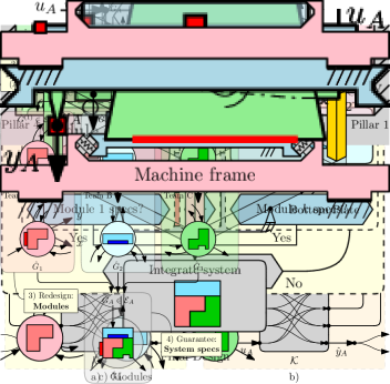
Figure 3: A schematic example of the modular modelling framework with a fixed interconnected structure $\mathcal{K}$ where a) given the original system model and b) the redesigned system model.

3 User-defined system FRF specifications

To enable the exploitation of the approach introduced in [janssen2023modular], we define FRF specifications on the dynamics of the system in the frequency domain. For the purpose of modular redesign, we pose the following definition for design specifications on the dynamic behaviour in the frequency domain:

Definition 1.

For FRF system specifications $\mathcal{E}_{A}(\omega)$ given by

$$\mathcal{E}_{A}(\omega) :=\Big{\{}\hat{G}_{A}(i\omega)\ \big{|}$$

$$\|V_{A}(\omega)(G_{A}(i\omega)-\hat{G}_{A}(i\omega))W_{A}(\omega)\|<1\Big{\}},$$ (19)

the redesigned modular system is considered to satisfy its specifications, denoted by $\hat{G}_{A}\in\mathcal{E}_{A}$, if and only if its FRF $\hat{G}_{A}(i\omega)\in\mathcal{E}_{A}(\omega)$ for all $\omega\in\Omega$. Here, $G_{A}(i\omega)$ is the original system FRF, and $V_{A}(\omega)$ and $W_{A}(\omega)$ are positive, diagonal, frequency-dependent scaling matrices, and $\omega$ is evaluated at the frequencies of interest, defined by $\Omega\subseteq\mathbb{R}$.

Remark 2.

In this paper, we denote the Euclidean norm or 2-norm of a matrix $A$ as $\|A\|$ which is equal to its largest singular value $\bar{\sigma}(A)$. If we denote $\|G(i\omega)\|$, we imply that we simply obtain the 2-norm of $G(i\omega)$ at each frequency $\omega$ which, for SISO systems, is identical to the magnitude of $G(i\omega)$.

Definition 1 imposes specifications on the system-level that are effectively a bound on the allowed change of the original FRF $G_{A}(i\omega)$ to the redesigned FRF $\hat{G}_{A}(i\omega)$ at specific frequency points. Here, the scaling matrices $V_{A}(\omega)$ and $W_{A}(\omega)$ are used to scale the allowed change in the dynamics of the system for each input-to-output pair at each $\omega\in\Omega$. This allows for a fully flexible redesign specification. To illustrate how these specifications restrict the allowed change in the dynamics from $G_{A}(i\omega)$ to $\hat{G}_{A}(i\omega)$, two equivalent representations of a specification on a SISO example FRF are shown in Figure 4. Note that for MIMO systems, Definition 1 still applies, but its meaning is difficult to visualize as (1) restricts all input-output pairs at the same time.

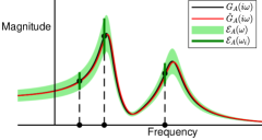
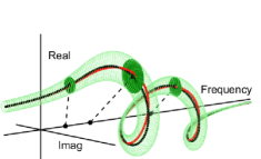
Figure 4: Two equivalent visualizations of an original system FRF $G_{A}(i\omega)$, specifications $\mathcal{E}_{A}(\omega)$, and a redesigned system FRF $\hat{G}_{A}\in\mathcal{E}_{A}$. In addition, three specific frequency points are highlighted to show that $\mathcal{E}_{A}(\omega)$ not only restricts the magnitude, but also the phase of $\hat{G}_{A}(i\omega)$.

Note that the overall system specification $\mathcal{E}_{A}(\omega)$ is user-defined, i.e., the system engineer can select the frequency points $\Omega$ and the corresponding weighting matrices $W_{A}(\omega)$ and $V_{A}(\omega)$. Practically, this means that the system engineer selects the frequency points and the radius of the circles visualized in Figure 4 at these frequencies. For example, a system engineer might consider specifications on the interconnected system that are a tight bound on the FRF at low frequencies and at frequencies that are prominent in the reference trajectories of the system in operation, while at other (higher) frequencies, a less restrictive specification is allowed.

4 Computation of module specifications with assembly specification guarantees

In this section, we will show 1) how the system FRF specifications $\mathcal{E}_{A}$ defined in Definition 1 can be used to automatically generate module FRF specifications $\mathcal{E}^{(j)}$ and 2) that if these specifications are satisfied for all modules, i.e., $\hat{G}^{(j)}\in\mathcal{E}^{(j)}$, then $\hat{G}_{A}\in\mathcal{E}_{A}$ is guaranteed. First, similar to the system specifications, we define the module specifications.

Definition 2.

For FRF module specifications $\mathcal{E}^{(j)}(\omega)$ given by

$$\mathcal{E}^{(j)}(\omega) :=\Big{\{}\hat{G}^{(j)}(\textrm{i}\omega)\ \big{|}$$

$$\|(W^{(j)}(\omega))^{-1}(\hat{G}^{(j)}-G^{(j)})(\textrm{i}\omega)(V^{(j)}(\omega))^{-1}\|\leq 1\Big{\}},$$ (20)

any redesigned module $j=1,2,\dots,k$ is considered to satisfy its FRF specifications, denoted by $\hat{G}^{(j)}\in\mathcal{E}^{(j)}$, if and only if its FRF $\hat{G}^{(j)}(i\omega)\in\mathcal{E}^{(j)}(\omega)$ for all $\omega\in\Omega$. Here, $G^{(j)}(i\omega)$ is the FRF of the original module $j$, and $V^{(j)}(\omega)$ and $W^{(j)}(\omega)$ are positive, diagonal, frequency-dependent scaling matrices, and $\omega$ is evaluated at the frequencies of interest, defined by $\Omega\subseteq\mathbb{R}$.

Note that the module specifications in Definition 2 have the same characteristics as the system specification in Definition 1. Namely, they allow for a maximum change in dynamics in the FRF $\hat{G}^{(j)}(\omega)$ with respect to $G^{(j)}(\omega)$ based on the values in the matrices $V^{(j)}(\omega)$ and $W^{(j)}(\omega)$.

To enable a modular redesign approach, we aim to relate the system specifications $\mathcal{E}_{A}$ to the module specifcations $\mathcal{E}^{(j)}$. To achieve this, we define the nominal system

$$N(i\omega) :=\left[\begin{array}[]{cc}\mathcal{K}_{BB}(I-G_{B}(i\omega)\mathcal{K}_{BB})^{-1}&(I-\mathcal{K}_{BB}G_{B}(i\omega))^{-1}\mathcal{K}_{BA}\\ \mathcal{K}_{AB}(I-G_{B}(i\omega)\mathcal{K}_{BB})^{-1}&O\end{array}\right],$$ (23)

which comprises only of the original modules and interconnection structure. Furthermore, based on the system and module specifications (1) and (2), respectively, we define

$$V(\omega) =\textrm{diag}\big{(}V^{(1)}(\omega),\dots,V^{(k)}(\omega),V_{A}(\omega)\big{)},\text{and}$$ (24)

$$W(\omega) =\textrm{diag}\big{(}W^{(1)}(\omega),\dots,W^{(k)}(\omega),W_{A}(\omega)\big{)}.$$ (25)

Then, we can pose the following theorem that relates the satisfaction of module specifications to the satisfaction of the assembly specification.

Theorem 1.

Consider the nominal system in (23) and the specification-related scaling matrices in (25). If there exists

$$(D_{\ell},D_{r})\in\mathbf{D}$$ (26)

such that

$$\left[\begin{array}[]{cc}W^{-2}(\omega)D_{r}^{-1}&N^{H}(\textrm{i}\omega)\\ N(\textrm{i}\omega)&V^{-2}(\omega)D_{\ell}\end{array}\right] \succ 0$$ (29)

holds, where, given that $I_{n}$ denotes an identity matrix of dimension $\mathbb{R}^{n\times n}$,

$$\mathbf{D} :=\Big{\{}(D_{\ell},D_{r})\ \Big{|}\ d_{1},\dots,d_{k},d_{A}\in\mathbb{R}_{>0},$$ (30)

$$\qquad\qquad D_{\ell}=\textrm{diag}\left(d_{1}I_{p_{1}},\dots,d_{k}I_{p_{k}},d_{A}I_{m_{A}}\right),$$

$$\qquad\qquad D_{r}=\textrm{diag}\left(d_{1}I_{m_{1}},\dots,d_{k}I_{m_{k}},d_{A}I_{p_{A}}\right)\Big{\}},$$

then, satisfaction of the module specifications for all $\omega\in\Omega$, i.e.,

$$\hat{G}^{(j)}\in\mathcal{E}^{(j)}$$ (31)

for all $j=1,2,\dots,k$, implies satisfaction of the system specifications for all $\omega\in\Omega$, i.e.,

$$\hat{G}_{A}\in\mathcal{E}_{A}.$$ (32)

Proof.

We can define

$$E^{(j)}(i\omega) =\hat{G}^{(j)}(i\omega)-G^{(j)}(i\omega),\textrm{ and}$$ (33)

$$E_{A}(i\omega) =\hat{G}_{A}(i\omega)-G_{A}(i\omega).$$ (34)

Therefore, by substituting (33) in (2) and (34) in (1), Theorem 1 becomes equivalent to the constraints of [janssen2022modeselect, Theorem 3.1] which in turns follows from [janssen2022modular, Theorem 3.4]. The proofs in [janssen2022modular] in turn follow from definitions on the upper bound on the structured singular value [packard1993complex], a mathematical tool used in the field of robust control. ∎

Theorem 1 gives a mathematical approach to verify whether module properties imply system properties, which is the core idea of this approach. However, note that the matrix inequality (23) is not linear in the parameters, $V$, $W$, $D_{\ell}$ and $D_{r}$ which makes it difficult to optimize over these parameters. We will propose an alternating optimization algorithm that alternates between solving two different linear matrix inequalities (LMIs) to obtain a solution. Specifically, Theorem 1 is used to optimize over the module weights $V^{(j)}$ and $W^{(j)}$ to allow for module redesigns with redesign spaces that are as large as possible. Therefore, in the following Algorithm 1, we show how Theorem 1 can be used to automatically generate a set of FRF-based specifications $\mathcal{E}^{(j)}(i\omega)$ for all modules $j=1,2,\dots,k$ for any $\omega\in\Omega$ on the basis of the assembly specification $\mathcal{E}_{A}(i\omega)$. An example of such a specification is given in Remark LABEL:rem:gamma.

Algorithm 1 Computation of Module Specification

Input: The original module model FRFs $G^{(j)}(i\omega)$ for all $j=1,2,\dots,k$ and interconnection structure $\mathcal{K}$ to obtain $N$ as in (23), and user-defined system specifications $\mathcal{E}_{A}(\omega)$ as in Definition 1 in terms of $V_{A}(\omega)$ and $W_{A}(\omega)$ for a discrete set of frequencies of interest $\omega\in\Omega$.

Initialize $D_{r}^{\star}:=I$, $D_{\ell}^{\star}:=I$, $i:=0$, and define a stopping criterion $\epsilon\ll 1$.

for all $\omega\in\Omega$ do

     repeat

         $i:=i+1$

          Fix $D_{r}^{\star}$, $D_{\ell}^{\star}$, $V_{A}(\omega)$ and $W_{A}(\omega)$, solve the following semi-definite optimization problem: $\displaystyle\begin{array}[]{ll}\min\limits_{{\color[rgb]{1,0,0}\beta_{i}}\in\mathbb{R}}&{\color[rgb]{1,0,0}\beta_{i}}:=\text{tr}\left({\color[rgb]{1,0,0}V^{-2}(\omega)}\right)+\text{tr}\left({\color[rgb]{1,0,0}W^{-2}(\omega)}\right),\\ \text{s.t.}&\left[\begin{array}[]{cc}{\color[rgb]{1,0,0}W^{\text{-}2}(\omega)}{D_{r}^{\star}}^{\text{-}1}&N^{H}(\textrm{i}\omega)\\ N(\textrm{i}\omega)&{\color[rgb]{1,0,0}V^{\text{-}2}(\omega)}D_{\ell}^{\star}\end{array}\right]\succ 0.\\ \end{array}$ (39) Note that here, $V$ and $W$ are as given in (24) and (25), respectively, and, as $V_{A}(\omega)$ and $W_{A}(\omega)$ are given, only $V^{(j)}(\omega)$ and $W^{(j)}(\omega)$ are optimization parameters. Define $V^{\star}(\omega)$, $W^{\star}(\omega)$ and $\beta_{i}^{\star}$ as the solution to the red optimization parameters in (39).

          Fix $V^{\star}(\omega)$, $W^{\star}(\omega)$, solve the following semi-definite optimization problem: $\displaystyle\begin{array}[]{ll}\min\limits_{{\color[rgb]{0,0.6,0}\delta_{i}}\in\mathbb{R}}&\begin{array}[]{rl}N(i\omega){(W^{\star}(\omega))}^{2}{\color[rgb]{0,0.6,0}D_{r}}N^{H}(i\omega)&\\ -{(V^{\star}(\omega))}^{-2}{\color[rgb]{0,0.6,0}D_{\ell}}&\prec{\color[rgb]{0,0.6,0}\delta_{i}},\end{array}\\ \text{s.t.}&({\color[rgb]{0,0.6,0}D_{\ell}},{\color[rgb]{0,0.6,0}D_{r}})\in\mathbf{D}.\end{array}$ (44) Define $D_{\ell}^{\star},D^{\star}_{r}$ and $\delta_{i}^{\star}$ as the solution to the green optimization parameters in (44), which in the next iteration allows for a further reduction of $\beta_{i}$.

     until $\beta_{i-1}^{\star}-\beta_{i}^{\star}<\epsilon$

end for

Output: Module specifications $\mathcal{E}^{(j)}(\omega)$ for all $\omega\in\Omega$ as in Definition 2 for all $j=1,2,\dots,k$ given the obtained $V^{(j)}(\omega)$ and $W^{(j)}(\omega)$ from (39) for which it holds that if $\hat{G}^{(j)}\in\mathcal{E}^{(j)}$ for all $j=1,2,\dots,k$, then $\hat{G}_{A}\in\mathcal{E}_{A}$ is guaranteed.