Generating Higher Order Modes from Binary Black Hole mergers with Machine Learning

Abstract

We introduce a machine learning model designed to rapidly and accurately predict the time domain gravitational wave emission of non-precessing binary black hole coalescences, incorporating the effects of higher order modes of the multipole expansion of the waveform. Expanding on our prior work [1], we decompose each mode by amplitude and phase and reduce dimensionality using principal component analysis. An ensemble of artificial neural networks is trained to learn the relationship between orbital parameters and the low-dimensional representation of each mode. We train our model on $\sim 10^{5}$ signals with mass ratio $q\in[1,10]$ and dimensionless spins $\chi_{i}\in[-0.9,0.9]$, generated with the state-of-the-art approximant SEOBNRv4HM. We find that it achieves a median faithfulness of $10^{-4}$ averaged across the parameter space. We show that our model generates a single waveform two orders of magnitude faster than the training model, with the speed up increasing when waveforms are generated in batches. This framework is entirely general and can be applied to any other time domain approximant capable of generating waveforms from aligned spin circular binaries, possibly incorporating higher order modes.

I Introduction

With almost a hundred of confirmed detections, gravitational wave (GW) astronomy is entering a mature state, where many loud GW events will force the scientific community to develop faster analyses to deliver precision measurements. Expanding on past results [2, 3, 4], the recent transient catalogue GWTC-3 [5] is the latest achievment of the effort carried on by the LIGO-Virgo-KAGRA collaboration [6, 7, 8, 9] and it relies on both instrument and data analysis development.

A crucial element of the data analysis is the ability to quickly and accurately generate waveforms for GW signals emitted by coalescing binary black holes (BBHs). Such waveforms are used for the expensive Bayesian estimation of the parameters characterizing a BBH [10]: the analysis of a single event requires the online generation of up to billions of waveforms. As we move towards the next generation of detectors, such as Einstein Telescope [11, 12] and Cosmic explorer [13, 14], it will become even more necessary to deploy accurate waveform models that are fast and, at the same time, incorporate the full physics of the problem, otherwise our analyses will become subject to systematic errors in the parameter recovery [15]. On the other hand, accurate models are often slow to generate on a computer and the analyses might struggle to keep up with the large event rate expected in the next-generation observatories [16]. Balancing the two needs is challenging, since speed and accuracy are often at trade.

An essential aspect for a realistic BBH signal model is the incorporation of higher-order modes (HMs) of the multipole expansion of the waveform [17]. For nearly equal mass systems, the leading-order mode is orders of magnitude larger than the others and, including the HMs does not significantly affect the parameter estimation. However, it has been demonstrated [18, 19, 20, 21] that HMs are observable in highly asymmetric binary systems. In fact, the effect of HMs has already been observed in at least two BBH events originating from asymmetric binaries [22, 23]. This underscores the importance of including HMs in any parameter estimation pipeline in order to avoid biases in the recovered parameters.

Two main families of models have been developed, both being able to incorporate HMs. One family relies on the Effective One Body (EOB) formalism [24, 25, 26, 27, 28, 29, 30, 31], which maps the complicated general relativistic binary system into a problem governed by an effective Hamiltonian. EOB models tend to be accurate but are quite costly to generate, since for each waveform one needs to solve the Hamiltonian equation of motion. On the other hand, the phenomenological waveforms [32, 33, 34] are based on analytical expressions, making use of the post-Newtonian formalism to model the inspiral, and on fits to numerical simulations to describe the intermediate and merger-ringdown regimes. They tend to be faster to evaluate than the EOB models. Both families, EOB and phenomenological, need to be calibrated with numerical relativity waveforms, computed by directly solving the Einstein equations in discretized form. The calibration makes sure that a model retains its accuracy even close to merger, where approximate treatments such as the the post-Newtonian or EOB formalisms are no longer applicable by themselves.

Besides the standard families, surrogate waveform models have been developed with the aim of reproducing the output of a target model and of making feasible the usage of the underlying model.

A first class of surrogates is designed to closely reproduce numerical relativity (NR) waveforms [35, 36, 37, 38, 39, 40, 41] and, accordingly, it is trained using only NR waveforms as input. NR surrogates are very accurate but they tend to be very short, due to the nature of the NR waveforms employed for training. For this reason, they are often hybridized using an analytical expression for the early inspiral.

Besides targeting NR waveforms, several surrogates have been developed to accelerate EOB models [42, 43, 44, 45, 46], even including HMs. While traditional surrogate models build an empirical interpolant on the waveform space, a more recent approach relies on performing a regression using machine learning techniques [47, 48, 49, 50].

Among others, [1] introduced a machine learning surrogate model, based on a dimensionality reduction scheme followed by a regression. In this work, we extend this model to HMs and we improve the accuracy of the regression. Our model marks a step towards the development of a faster, yet precise, waveform model, and will help enable the accurate analysis of next-generation detector data.

We train our model on the widely used approximant SEOBNRv4HM [26] to target systems with mass ratio $q\in[1,10]$ and dimensionless spin components between $[-0.9,0.9]$ and we achieve a $10^{-4}$ median faithfulness (with tails up to $10^{-2}$) when averaged across a wide range in parameter space. Our numerical experiments show that our model offers a substantial speed-up with respect to the original model, matching the speed of the state-of-the-art surrogate models.

This paper is organized as follows. In Sec. II we introduce the details of the model presented here, stressing the differences with the model in [1]. Sec. III is devoted to the validation of our model: we will motivate our choice of several hyperparameters and perform an accuracy and speed study. In Sec. IV, we present some final remarks and highlight future perspectives.

II Building the model

A non-precessing BBH can be described by four intrisic parameters, which specify the two BH masses $m_{1}$ and $m_{2}$ and the z-components of the two dimensionless spins, $\chi_{\text{1z}}$ and $\chi_{\text{2z}}$. Since the total mass $M=m_{1}+m_{2}$ acts as a scaling parameter, when generating non-precessing BBH signals one only needs to consider the mass ratio $q=m_{1}/m_{2}\geq 1$ together with the spins. We refer to the relevant parameters as $\bm{\vartheta}=(q,\chi_{\text{1z}},\chi_{\text{2z}})$. Besides the masses and spins, the gravitational wave emitted by the system depends also on luminosity distance to the source $d_{L}$, the inclination angle $\iota$ of the source, and the reference phase $\varphi_{0}$; these are the extrinsic parameters.

As is standard, we expand the angular dependence on $\iota,\varphi_{0}$ of the complex waveform $h(t)$ in terms of a sum of spin -2 spherical harmonics. A GW is then parameterized as [51]:

$$h(t;d_{L},\iota,\varphi_{0},m_{1},m_{2},\chi_{\text{1z}},\chi_{\text{2z}})=h_{+}+ih_{\times}$$

$$\qquad=\frac{G}{c^{2}}\frac{M}{d_{L}}\sum_{\ell=2}^{\infty}\sum_{m=-\ell}^{\ell}\tensor{[}^{-2}]{Y}{{}_{\ell m}}(\iota,\varphi_{0})h_{\ell m}(t/M;\bm{\vartheta}),$$ (1)

where we refer to the functions $h_{\ell m}(t;\bm{\vartheta})$ as modes of the waveform. We note that that, for non-precessing systems, $h_{\ell m}=(-1)^{\ell}h^{*}_{\ell-m}$, hence we will only consider modes with $m>0$.

The mode $(\ell,m)=(2,2)$ is the largest in amplitude, hence it is often referred to as the dominant mode. The other sub-dominant modes are usually few orders of magnitude smaller in amplitude and become more relevant (and measurable) for high mass ratios [21, 22, 23].

In this work, we introduce a machine learning model to perform a regression

$$(q,\chi_{\text{1z}},\chi_{\text{2z}}) \longmapsto h_{\ell m}(t;\bm{\vartheta})$$ (2)

for each mode $(\ell,m)$. The regression is designed to reproduce waveforms from a given data set; such waveforms can be generated by any time-domain approximant.

We decompose each mode in an amplitude term $A_{\ell m}$ and a phase term $\phi_{\ell m}$ as follows:

$$h_{\ell m}(t;\bm{\vartheta})=A_{\ell m}(t;\bm{\vartheta})e^{i\phi_{\ell m}(t;\bm{\vartheta})},$$ (3)

and, for each mode, we perform a regression for amplitude and phase separately. The regression scheme closely follows [1] and relies on:

1. A suitable vector representation of the regression target by choosing a fixed time grid;

2. A principal component analysis (PCA) model to reduce the dimensionality of each waveform;

3. An artificial neural network (ANN) regression to learn the dependence on $\bm{\vartheta}$ of the reduced waveform.

While the first two elements are unchanged from the previous work, the ANN regression is first introduced here. Indeed a NN has more representation power than the Mixture of Experts (MoE) model [52], used in [1]: the change was needed to achieve better accuracy for the model.

II.1 Data set creation

To construct a data set, we follow [1] and we set a dimensionless time grid. We construct the grid by setting $D$ points equally spaced in $\tau^{\alpha}$, where $\tau$ is the physical time scaled by the total mass of the system $M$: $\tau=t/M$. Using the findings of [1], we set $D=\text{2000}$ and $\alpha=\text{0.5}$. This is a good compromise between the need of having a faithful representation of the waveform (which requires a large grid) and the need of having a compact model (which points to a sparse grid). The waveforms are time-shifted so that the peak of the amplitude of the $(2,2)$ mode happens at $\tau=0$. The grid starts at (scaled) time $\tau_{\text{min}}=-\tau_{0}$, where $\tau_{0}$ sets the length of the waveform that our model is able to generate (as a function of the total mass $M$). We choose $\tau_{0}=$2\text{\,}\mathrm{s}\mathrm{/}\mathrm{M}_{\odot}$$ and we populate the data set with $68000$ waveforms.

To make sure that the distribution of $q$ is skewed towards towards the boundaries, where the regression is less accurate, we sample the mass ratio $q$ in the range $[1,10]$ with the following procedure:

• We sample $q_{1},\ldots,q_{5}\sim\mathcal{U}_{[1,10]}$;

• We sample $x\sim\mathcal{U}_{[0,1]}$;

• We select $q$, based on the value of $x$:

  • If $x\in[0,0.3)$, $\min q_{1},\ldots,q_{5}$,

  • If $x\in[0.3,0.8)$, $q_{1}$,

  • If $x\in[0.8,1]$, $\max q_{1},\ldots,q_{5}$,

where $\mathcal{U}_{[a,b]}$ is the uniform distribution in $[a,b]$. The spins are drawn uniformly in the range $[-0.9,0.9]$.

Once a time grid is set, we evaluate all the modes (amplitude and phase) on the time grid and represent them as vectors in $\mathbb{R}^{D}$. We then create a data set $\{X,Y\}$ of $N$ elements. Each row of the data set is of the form:

$$X =[q,\chi_{\text{1z}},\chi_{\text{2z}}]$$ (4)

$$Y =[\bm{A}^{T}_{\ell m},\bm{\phi}^{T}_{\ell m},\ldots]$$ (5)

The data set $Y$ gathers the amplitude and phase for the different modes in the data set. We include all the modes available in SEOBNRv4HM: $(\ell,m)=\{(2,2),(2,1),(3,3),(4,4),(5,5)\}$.

In what follows we will refer to any of the vectors $\bm{A}_{\ell m}$ or $\bm{\phi}_{\ell m}$ as $\bm{f}$. Note that we use the same grid for all the modes.

II.2 Dimensionality reduction

It is unfeasibile to perform a regression targeting a high-dimensional vector such as $\bm{f}\in\mathbb{R}^{D}$. For this reason, in [1] we introduced a principal component analysis (PCA) dimensionality reduction scheme. It is an approximately invertible linear mapping between a vector $\bm{f}\in\mathbb{R}^{D}$ in a large dimensional space to lower dimensional vector $\bm{g}\in\mathbb{R}^{K}$:

$$\mathbf{g}=H(\mathbf{f}-\bm{\mu}),$$ (6)

$$\hat{\mathbf{f}}=H^{T}\mathbf{g}+\bm{\mu},$$ (7)

where $\bm{\mu}\in\mathbb{R}^{D}$ and $H$ is a $K\times D$ matrix. The rows $H_{i:}$ of $H$, also called principal components (PC), form an orthonormal set of vectors, i.e. ${\sum_{k=1}^{D}H_{ik}H_{kj}=\delta_{ij}}$. The PCs are the first $K$ eigenvectors of the $D\times D$ covariance matrix of the data set, as described in [53, Sec. 12].

The mapping is only approximately invertible, in the sense that $\hat{\mathbf{f}}$ is only an approximation of the high dimensional vector $\mathbf{f}$. The quality of the approximation is controlled by the number $K$ of PCs considered: the more PCs, the more accurate the reconstruction of $\mathbf{f}$ is.

One can have a deeper insight on PCA considering the following formula for the reconstructed vector $\hat{\mathbf{f}}$ (setting $\bm{\mu}=0$ without loss of generality):

$$\hat{\mathbf{f}}=\sum_{i=0}^{K-1}\langle\mathbf{f}|H_{i:}\rangle\;H_{i:}$$ (8)

where $\langle\mathbf{a}|\mathbf{b}\rangle=\sum_{i=0}^{D-1}a_{i}b_{i}$ is the Euclidean scalar product between two vectors $\mathbf{a},\mathbf{b}\in\mathbb{R}^{D}$. Since less important PCs are more orthogonal to data, the typical magnitude of $g_{i}=\langle\mathbf{f}|H_{i:}\rangle$ decreases as $i$ increases.. As a consequence, the regression for a lower order PC needs to be more accurate than the one for the higher order PC. This will be taken care of by a suitable choice for the loss function for the regression (see next section).

Following [1], in this work we employ for each mode $6$ PCA compontents for the phase model and $4$ for the amplitude. While it’s plausible that an optimal number of components may vary for different modes, we opt for simplicity by employing the same number of PCA components for all modes, a configuration tuned based on the $(2,2)$ mode only.

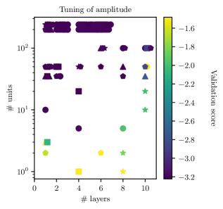
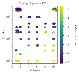
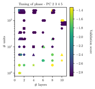
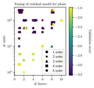
Figure 1: Results from the validation of our ANN models, using the $\ell,m=2,2$ mode data set. We tune the number of layers and the number of features per layer, together with the features and the polynomial order for the data augmentation. Each panel in the figure refers to a different ANN, taking care of different parts of the regression, as described in Sec. II.3. For each regression, we train 100 ANNs with different choices of hyperparameters. Each point in the plot, refers to a trained network and it is colored with the logarithm of the loss function computed on the validation data, referred to as the validation score. Note that we do not report the features used for data augmentation, so that the plot is degenarate in this quantity.

II.3 Neural network regression

An artificial neural network (ANN) is a popular regression model, consisting of a powerful parametric function, whose parameters (or weights), when properly set, can represent a large variety of relations between input and output [54, 53, 55]. An ANN is built by stacking together $N_{\text{L}}$ layers in such a way that the output of a layer is the input of the following layer. Each layer is a function $L:\mathbb{R}^{D^{\prime}}\rightarrow\mathbb{R}^{D^{\prime\prime}}$ and has the following functional form:

$$\bm{y}=a(W^{\prime}_{\prime\prime}\bm{x})$$ (9)

Where $W^{\prime}_{\prime\prime}$ is a $D^{\prime\prime}\times D^{\prime}$ matrix and $a:\mathbb{R}\rightarrow\mathbb{R}$ is an activation function that acts element-wise on the vector $W^{\prime}_{\prime\prime}\bm{x}$. Each component $y_{i}$ of the output of the layer is called a node and the number of nodes is a tunable parameter, controlling the representative power of the layer.

An ANN $\mathcal{N}$ is obtained by composing $N_{\text{L}}$ different layers (each with a suitable number of nodes):

$$\mathcal{N}_{W}=L_{N_{\text{L}}}\circ\ldots\circ L_{2}\circ L_{1}$$ (10)

where we denote by $W$ the set of all the parameters the ANN depends on.

The number of layers, together with the number of nodes per layer are hyperparameters that need to be carefully chosen, to balance model accuracy and model complexity. Another important choice is the activation function: several possible choices are possible, the most popular being the sigmoid, the hyperbolic tangent or the so called ReLU function. In our work, we consider the sigmoid function between all layers, except for the very last layer which has linear/identity activation so that negative values are also possible.

Once the ANN is set up, we need to set its weights to the values that achieve our regression task. This procedure is called training, where we minimize a loss function with respect to the weights $\bm{W}$ of the model. The loss function depends on the data set at hand ${\{\bm{x}_{i},\bm{y}_{i}\}}$. Mathematically, the weights are given by:

$$\bm{W}=\operatorname*{arg\,min}_{W}\mathcal{L}(W;\{\bm{x}_{i},\bm{y}_{i}\}_{i})$$ (11)

The minimization of the loss function is performed by stochastic gradient descent (SGD), as implemented by the Nadam algorithm [56], which combines the popular Adam algorithm [57] with the Nesterov momentum. The optimization relies on the gradients $\partial_{W}\mathcal{L}$ of the loss function, computed through the back-propagation algorithm [58].

To perform our regression $\theta\longmapsto\bm{g}$, we employ an ensemble of networks that suitably combined delivers accurate results. To improve the representative power or the ANN, we employ feature augmentation on the vector $\bm{\vartheta}=(q,\chi_{\text{1z}},\chi_{\text{2z}})$, effectively using the augmented vector $\tilde{\bm{\vartheta}}$ as input for the regression. Although different ANN’s will need different features, we will for convenience abuse the notation $\tilde{\bm{\vartheta}}$ to denote any augmented vector. Indeed, the features to add need to be chosen with a validation process: this will be discussed in the next section.

Before the training, the regression targets $\bm{y}_{i}$ are scaled such that $\bm{y}_{i}\rightarrow\frac{\bm{y}_{i}}{\bm{w}}$, where $\bm{w}$ keeps the maximum of $|\bm{y}_{i}|$ along each axis. In this way all the regression targets span the same order or magnitude, facilitating the “learning” task.

For the amplitude $\bm{A}_{\ell m}$ of each mode, we employ a single ANN $\mathcal{N}_{A_{\ell m}}$ that predicts the first four PCA components. The predicted amplitude $\hat{\bm{A}}_{\ell m}$, including the PCA reconstruction, has the following form:

$$\hat{\bm{A}}_{\ell m}(\bm{\vartheta})=\bm{\mu}_{A_{\ell m}}+H_{A_{\ell m}}^{T}\mathcal{N}_{A_{\ell m}}(\tilde{\bm{\vartheta}}).$$ (12)

For the phase $\bm{\phi}_{\ell m}$, we employ one ANN $\mathcal{N}_{\phi_{\ell m}\text{- 01}}$ to predict only the first two PCA components. Another ANN will take care of the remaining components $\mathcal{N}_{\phi_{\ell m}\text{- 2345}}$. On top of this, we build an additional ANN $\mathcal{N}_{\phi_{\ell m}\text{- residual}}$ to target the residual of the predictions of $\mathcal{N}_{\phi_{\ell m}\text{- 01}}$. The scheme makes sure that the first two PCs are predicted with much larger accuracy than the others. Indeed, the reconstructed WF depends largely on the first two components and a small fractional error can potentially have a large impact on the overall accuracy.

The predicted phase $\hat{\bm{\phi}}_{\ell m}$ is then given by

$$\hat{\bm{\phi}}_{\ell m}(\bm{\vartheta}) =\bm{\mu}_{\phi_{\ell m}}+$$

$$H_{\phi_{\ell m}}^{T}\begin{pmatrix}\mathcal{N}_{\phi_{\ell m}\text{- 01}}(\tilde{\bm{\vartheta}})+\mathcal{N}_{\phi_{\ell m}\text{- residual}}(\tilde{\bm{\vartheta}})\\ \mathcal{N}_{\phi_{\ell m}\text{- 2345}}(\tilde{\bm{\vartheta}})\hfill\end{pmatrix}$$ (13)

We train our model using the PCA data set, obtained by PCA reducing the training set. Each ANN is trained using the following loss function:

$$\mathcal{L}=\frac{1}{N}\sum_{i=1}^{N}\Bigl{(}(\mathcal{N}(\bm{\vartheta}_{i})-\bm{y}_{i})\Bigr{)}^{2}\;\bm{w},$$ (14)

where $\bm{y}_{i}$ is the (scaled) regression target of each network and $\bm{w}\in\mathbb{R}^{K}$ takes into account the fact that different PCs have different orders of magnitude.

The network is implemented and trained using the python package keras [59], built on tensorflow backend [60].

III Performance study

In this section, we first study how the model performance depends on the different choices of hyperparameters (network architecture, learning rate, features, …). The architecture details of the model (chosen after hyperparameters tuning) are reported in Tab. 1. We then evaluate the faithfulness of our model and report the speed up that we obtain when using our surrogate instead of the training model SEOBNRv4HM. In what follows, we will refer to our model as mlgw-SEOBNRv4HM.

To measure the discrepancy between two waveforms $h_{1}$, $h_{2}$, we define a scalar product

$$(h_{1}|h_{2})=4\Re\int_{0}^{\infty}\text{d}f\;\frac{{\tilde{h}^{*}}_{1}(f)\tilde{h}_{2}(f)}{S_{n}(f)},$$ (15)

where $\tilde{\phantom{h}}$ denotes the Fourier transform and $S_{n}(f)$ is the power spectral density (PSD) of the detector’s noise. We can use the scalar product to arrive at a normalized waveform, $\hat{h}=\frac{h}{\sqrt{(h|h)}}$.

To measure the discrepancy between two individual modes $h^{1}_{\ell m}$ and $h^{2}_{\ell m}$, we define the match $\mathcal{M}$:

$$\mathcal{M}=\max_{t,\phi}\;(\hat{h}^{1}_{\ell m}|\hat{h}^{2}_{\ell m}e^{i2\pi ft+i\varphi})$$ (16)

where $he^{i2\pi ft+i\varphi}$ denotes (with a slight abuse of notation) $h$ translated in time by a factor of $t$ and with its phase shifted by $\varphi$. We call mismatch the quantity $\mathcal{F}=1-\mathcal{M}$.

The match defined above amounts to the search statistics being used for matched filtering searches of non-precessing/non-HM signals [61]. A different statistic is needed to search for HM signals, hence the match defined above is not suitable to compare two different waveforms with HM content as in Eq. (II). In this case, we need to compare the two polarizations $h_{+}$, $h_{\times}$ of a waveform with a signal $s$ observed at the detector:

$$s=F_{+}h_{+}+F_{\times}h_{\times},$$ (17)

where $F_{+},F_{\times}$ are called antenna pattern functions, depending on the sky location of the source and on the polarization angle [17].

Following [62], we introduce the symphony match between a signal $s$ and a waveform $h$:

$$\mathcal{M}_{\mathrm{sym}}=\max_{t}\;\frac{(\hat{s}|\hat{h}_{+})^{2}+(\hat{s}|\hat{h}_{\times})^{2}-2(\hat{h}_{\times}|\hat{h}_{+})(\hat{s}|\hat{h}_{+})(\hat{s}|\hat{h}_{\times})}{1-(\hat{h}_{\times}|\hat{h}_{+})^{2}}.$$ (18)

Note that $\mathcal{M}_{\mathrm{sym}}$ depends on the signal $s$, hence it depends on the sky location and polarization angle. As above, we define the symphony mismatch as $\mathcal{F}_{\mathrm{sym}}=1-\mathcal{M}_{\mathrm{sym}}$.

In what follows, we always use a constant (i.e. flat) PSD. While this certainly does not correspond to any actual detector, it makes sure that all the frequencies are weighted equally, hence giving a detector agnostic measure of the mismatch.

III.1 Hyperparameter tuning

Network	n-layers	units	features	order
$\mathcal{N}_{A_{\ell m}}$	1	35	$\mathcal{M}_{c},\chi_{\text{eff}}$	1
$\mathcal{N}_{\phi_{\ell m}\text{- 01}}$	2	50	$\mathcal{M}_{c},\eta,\log q,\chi_{\text{eff}}$	3
$\mathcal{N}_{\phi_{\ell m}\text{- 2345}}$	1	50	$\mathcal{M}_{c},\eta,\log q,\chi_{\text{eff}}$	1
$\mathcal{N}_{\phi_{\ell m}\text{- residual}}$	5	50	$\mathcal{M}_{c},\eta,\log q,\chi_{\text{eff}}$	2

Table 1: Architecture of the 4 ANNs employed to generate each mode. For each ANN we report the number of layers and the number of units per layer. We perform data augmentation by adding all the polynomials terms in the chosen features. The architecture has been chosen after hyperparameter tuning (see Fig. 1). Among other features, we use the chirp mass $\mathcal{M}_{c}=\frac{(m_{1}m_{2})^{3/5}}{(m_{1}+m_{2})^{1/5}}$, the symmetric mass ratio $\eta=\frac{m_{1}m_{2}}{(m_{1}+m_{2})^{2}}$ and the effective spin parameter $\chi_{\text{eff}}=\frac{m_{1}\chi_{\text{1z}}+m_{2}\chi_{\text{2z}}}{m_{1}+m_{2}}$

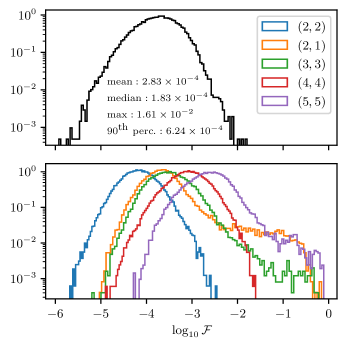
Figure 2: We report the results of the mismatch between the $50000$ test waveforms produced by mlgw-SEOBNRv4HM and by the training model SEOBNRv4HM. In the top panel, we report the histogram of the “symphony” mismatch $F_{\text{sym}}$ for the overall waveforms, where we compare the $h_{+}$ and $h_{\times}$ polarizations (see Eq. (8)). For the computation, we set random sky location. We also report the median, the mean and the maximumum mismatch, together with the value of the $90^{\text{th}}$ percentile. In the bottom panel, we report the histograms for the mismatches computed mode by mode. The composition of the test set is described in the text.

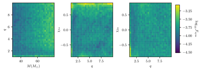
Figure 3: Depency of the “symphony” mismatch $F_{\text{sym}}$ between mlgw-SEOBNRv4HM and the training model SEOBNRv4HM, as a function of some chosen orbital paramers. The mismatch is computed on the $50000$ waveforms on the test set described in the text. On the left plot, we display the quantities $M-q$ on the two axis, while on the center and left plot we show on the axis the variables $q-\chi_{\text{1z}}$ and $q-\chi_{\text{2z}}$ respectively. Each bin is colored according to the average mismatch and the three plots shares the same color scale. We note that mlgw-SEOBNRv4HM’s faithfulness tends to decreases for low values of $q$ and large positive values of $s_{\text{1z}}$.

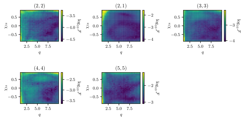
Figure 4: For each mode, we report the mismatch between mlgw-SEOBNRv4HM and the training model SEOBNRv4HM, as a function of $q$ and $s_{\text{1z}}$. The mismatch is computed on the $50000$ waveforms on the test set described in the text. Each bin is colored according to the average mismatch. We note that the performance between different modes can vary significantly and in general they decrease for low values of $q$ and high values of spins.

The performance of the model depends on a number of crucial choices about some non-trainable parameters, usually called hyperparameters. The hyperparameters define the architecture of the ANN as well as some parameters relevant to the training. Setting the right values for the hyperparameters is crucial for the ANN performance, as one needs to balance between accuracy and speed; this procedure is called hyperparameter tuning and can be done automatically to optimize manual work and to make sure to find a good minimum.

We optimize the following hyperparameters:

• n-layers: number of hidden layers in the ANN;

• units: number of nodes per hidden layer;

• features: features to use for data augmentation;

• order: the data will be augmented with all the monomials of the chosen features up the given order.

For each of the 4 ANN useful to produce a single mode (see Eqs. (12-13)), we train a network for different combinations of hyperparameters. The figure of merit of each hyperparameter choice is the logarithm of the loss function (see Eq. (14)) evaluated on the validation set. For our experiments we only use the data set of the $(2,2)$ mode and we employ the package keras-tuner [63].

We report our results in Fig. 1, where each combination of hyperparameters tested is represented in the n-layers-units plane and colored by the validation score. We can see that all the four ANN share the same trend: the most effective way to improve regression accuracy is to increase the number of units as opposed to the number of layers. The number of layers is far more important the extra features added and the polynomial order for data augmentation.

Furthermore, we note that the regressions for the amplitude and for the high phase PCs (i.e. components 2,3,4,5) can be performed with a smaller model, compared to the models for the first two PCs of the phase. This can be explained by the fact that most of the physical information is stored in the first two components of the phase, making this a harder regression problem.

In table Tab. 1 we report the final hyperparameter choice we made for each of the networks. The architectures are the same across the different modes considered.

As discussed above, we note that models $\mathcal{N}_{A_{\ell m}}$ and $\mathcal{N}_{\phi_{\ell m}\text{- 2345}}$ are very simple, having only one layer and a small polynomial order, while the other ANNs have a more complicated architecture. We note here that an accurate ANN for the residuals of the phase is crucial to obtain a good accuracy: indeed $\mathcal{N}_{\phi_{\ell m}\text{- residual}}$ is the most complex model we employ, meaning that the residual phase data set is the “hardest” to learn.

III.2 Accuracy study

To test the accuracy of our model, we generate a test set with $50000$ randomly chosen waveforms generated with the training model SEOBNRv4HM. The waveforms masses are characterized by a total mass in the range $[30,80]M_{\odot}$, by a mass ratio $q\in[1,10]$. The spins are chosen in the range $[-0.9,0.9]$ and the inclination angle $\iota$ and reference phase $\varphi_{0}$ are drawn uniformly from a sphere. We sample the starting frequency uniformly in the range $[10,20]$ Hz.

In Fig. 2, we report the histogram of the distribution of the mismatches between mlgw-SEOBNRv4HM and the test waveforms. The upper part refers to the mismatches Eq. (18) computed on the overall waveforms (with sky location sampled uniformly over the sky); the lower box refers to mismatches computed mode by mode with Eq. (16).

First of all, we note that the model shows very high faithfulness. With a median value of $2\times 10^{-4}$ and with virtually no signals with a “symphony” mismatch higher than $10^{-2}$, the accuracy of mlgw-SEOBNRv4HM matches the accuracy of other state-of-the-art surrogate models [45, 48, 46] and the accuracy of the training model SEOBNRv4HM in reproducing numerical relativity waveforms [26]. The faithfulness for the $(2,2)$ mode is even higher, with no signals whose mismatch exceeds $2\times 10^{-3}$. On the other hand, the higher order modes are less accurately reproduced than the dominant mode. In particular, for the modes $(2,1),(3,3),(5,5)$ a limited number of waveforms show very high mismatches $\mathcal{O}(1)$. See below for more discussion.

In Fig. 3 we report the dependence of the “symphony” mismatch as a function of the different orbital parameters. From the figure, it is manifest that the model has very stable performance across the parameter space. The faithfulness decreases for high positive values of the spin of the first object $s_{\text{1z}}$ and for mass ratio $q\sim 1$. Despite this, in such “extreme” regions, the average mismatch is still of the order of $10^{-4}$. The performance of the regression doesn’t depend on $\chi_{\text{2z}}$, since the quantity plays a very little role in defining the waveform features.

In Fig.4, for each mode we report the mismatch as a function of the mass ratio and of $s_{\text{1z}}$. One more time, we can see that the model faithfulness decreases for low mass ratios and for high spins. Moreover, the subdominant modes shows a poorer performance as compared to the dominant one: this was already observed in Fig. 2.

The observed decrease in faithfulness for sub-dominant modes needs some attention. As seen in Fig. 4, this decreased performance is consistently observed for low values of the mass ratio $q$. In systems with $q\sim 1$, it is well-known that the amplitude of the subdominant modes vanishes and hence they correspond to “outliers” in the data set. This clearly poses a challenge for both the PCA and the regression model for the amplitude, since modelling such a sharp feature of the data requires an enhanced model flexibility and many more training examples.

A mitigation strategy could involve introducing a $q$-dependent amplitude scaling for the waveforms before adding them to the data set. This approach would result in a data set with amplitude time series of approximately the same magnitude, reducing the outlier nature of waveforms with $q\sim 1$. Another straightforward strategy could deploy a larger network for such modes. Indeed, we tuned the hyperparameters on the $(2,2)$ mode (an “easy” regression target). Performing a network tuning on the data set of HMs might reveal that our chosen architecture is not optimal.

Finally, we note that since for $q\sim 1$, the sub-dominant modes have a vanishing amplitude, a large mismatch in the sub-dominant mode for $q\sim 1$ has very little impact on the overall waveform Eq. (II), as shown in Fig. 2. This explains why the overall mismatch is low, despite high mismatch for the HMs in some edge cases.

III.3 Timing study

A speed-up in the waveform generation is the main motivation to build a ML waveform generator; for this reason it is crucial to assess the gain in waveform generation time. For this reason, we use our test set to measure the ratio between the time to generate a waveform with SEOBNRv4HM and mlgw-SEOBNRv4HM. Our model offers further speed by generating waveform in batches: in this case, some operations are efficiently parallelized and happen more efficiently. We report our findings in Fig. 5.

We achieve a speed-up between a factor of $100$ and $200$, depending on the waveform. The speed up can be twice as much, ranging between $200$ and $400$, when waveforms are generated in batches of $100$.

The speed up achieved by mlgw-SEOBNRv4HM is comparable to the one obtained by the SEOBNRv4HM_ROM surrogate model [45], which is the state-of-the-art frequency domain surrogate model trained on SEOBNRv4HM. SEOBNRv4HM_ROM is obtained with standard techniques and it achieves a speed up ranging between 100 and 200. The two results might not be directly comparable, since the comparison for SEOBNRv4HM_ROM is performed in frequency domain and this involves computing the Fourier tranform of the SEOBNRv4HM waveform. As we perform the comparison in time domain, we omit the latter step, possibly obtaining lower values for the speed up as the ones obtained in [45].

On the other hand, the speed up achieved by mlgw-SEOBNRv4HM is slightly larger than the one obtained by the time domain surrogate model SEOBNRv4PHMSur [46]. Indeed, the authors report a speed up always lower than $100$. However, also in this case, the comparison might be biased because the latter study also considers the effects of precession.

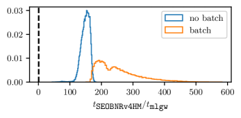
Figure 5: Speed up provided by mlgw-SEOBNRv4HM over the training model SEOBNRv4HM. In the histogram, we report the ration between the time $t_{\texttt{SEOBNRv4HM}}$ and the time $t_{\texttt{mlgw}}$ taken by the two models to generate each of the waveform in the test set. We note that mlgw-SEOBNRv4HM offers a speed up between a $100$ and $200$ with respect to the training model. mlgw-SEOBNRv4HM offers the option to generate waveforms in batches, effectively parallelizing some linear algebra operations. As shown in the plot, the batch generation provides a speed up of roughly a factor of two as compared with the non-parallelized version.

IV Final remarks and future prospects

Building on our previous work [1], we generate a ML surrogate model mlgw-SEOBNRv4HM able to reproduce with very high fidelity the output of the widely used approximant SEOBNRv4HM. mlgw-SEOBNRv4HM can generate waveforms in a cuboid $q\times\chi_{\text{1z}}\times\chi_{\text{2z}}=[1,10]\times[-0.9,0.9]\times[-0.9,0.9]$ on a (reduced) time grid of maximum length of $2\text{\,}\mathrm{s}\mathrm{/}\mathrm{M}_{\odot}$. Our model offers a two orders of magnitude speed up over the training model, without trading for accuracy, hence it is an attractive alternative for any data analysis application. Our method is fully general and is applicable to any chirp-like gravitational wave signal. To encourage new applications, we release our code (and our trained model) publicly as a python package through the PyPI repository.

Future work should also include precession. This can be achieved by means of the spin twist procedure [64, 65, 33, 66]. It consist on a time dependent rotation of the plane of emission, resulting in a phase and amplitude modulation which approximates the effect of precession. Training an ANN to predict the time dependent rotation is a promising step towards a complete ML surrogate model.

While the model is already applicable for most of the parameter estimation problems with current detectors, it is desirable to increase its range of validity, both in parameter space and in time span.

In principle, such an extension should be straightforward with the current network setup. On the other hand, due to an increased complexity of the regression task, probably more flexible architetures should be explored, using layers of different size. This would require a more careful (and computationally expensive) hyperparameters tuning.

An enhanced architecture should also benefit from sharing some parameters between models for different HMs - or even from treating the regression of the different modes as a large single regression problem. Indeed, the shapes of the different modes are correlated: for instance, the phases of two HMs are approximately proportional to each other. With the current architecture, the regression for each mode is carried on separately, hence each ANN needs to learn the WF behaviour independently. This could results in many redudant parameters in the network ensemble we introduced here. Inserting parameter sharing inside the regression setup could result in a lighter ANN, which would lead to a reduced inference time.

Similar improvements will become mandatory for the next generation detectors [15], when fast and reliable waveform models will be needed to mitigate the huge computational cost posed by very long observed waveforms. Our framework is ideal to achieve such an ambitious goal.

- [1] S. Schmidt, M. Breschi, R. Gamba, G. Pagano, P. Rettegno, G. Riemenschneider, S. Bernuzzi, A. Nagar, and W. Del Pozzo, “Machine Learning Gravitational Waves from Binary Black Hole Mergers,” Phys. Rev. D, vol. 103, no. 4, p. 043020, 2021.
- [2] B. P. Abbott et al., “GWTC-1: A Gravitational-Wave Transient Catalog of Compact Binary Mergers Observed by LIGO and Virgo during the First and Second Observing Runs,” Phys. Rev. X, vol. 9, no. 3, p. 031040, 2019.
- [3] R. Abbott et al., “GWTC-2: Compact Binary Coalescences Observed by LIGO and Virgo During the First Half of the Third Observing Run,” Phys. Rev. X, vol. 11, p. 021053, 2021.
- [4] R. Abbott et al., “GWTC-2.1: Deep extended catalog of compact binary coalescences observed by LIGO and Virgo during the first half of the third observing run,” Phys. Rev. D, vol. 109, no. 2, p. 022001, 2024.
- [5] R. Abbott et al., “GWTC-3: Compact Binary Coalescences Observed by LIGO and Virgo during the Second Part of the Third Observing Run,” Phys. Rev. X, vol. 13, no. 4, p. 041039, 2023.
- [6] B. P. Abbott et al., “Prospects for observing and localizing gravitational-wave transients with Advanced LIGO, Advanced Virgo and KAGRA,” Living Rev. Rel., vol. 21, no. 1, p. 3, 2018.
- [7] J. Aasi et al., “Advanced LIGO,” Class. Quant. Grav., vol. 32, p. 074001, 2015.
- [8] F. Acernese et al., “Advanced Virgo: a second-generation interferometric gravitational wave detector,” Class. Quant. Grav., vol. 32, no. 2, p. 024001, 2015.
- [9] T. Akutsu et al., “Overview of KAGRA: Detector design and construction history,” PTEP, vol. 2021, no. 5, p. 05A101, 2021.
- [10] J. Veitch et al., “Parameter estimation for compact binaries with ground-based gravitational-wave observations using the LALInference software library,” Phys. Rev., vol. D91, no. 4, p. 042003, 2015.
- [11] M. Punturo et al., “The Einstein Telescope: A third-generation gravitational wave observatory,” Class. Quant. Grav., vol. 27, p. 194002, 2010.
- [12] M. Maggiore et al., “Science Case for the Einstein Telescope,” JCAP, vol. 03, p. 050, 2020.
- [13] D. Reitze et al., “Cosmic Explorer: The U.S. Contribution to Gravitational-Wave Astronomy beyond LIGO,” Bull. Am. Astron. Soc., vol. 51, no. 7, p. 035, 2019.
- [14] M. Evans et al., “A Horizon Study for Cosmic Explorer: Science, Observatories, and Community,” 9 2021.
- [15] M. Pürrer and C.-J. Haster, “Gravitational waveform accuracy requirements for future ground-based detectors,” Phys. Rev. Res., vol. 2, no. 2, p. 023151, 2020.
- [16] A. Samajdar, J. Janquart, C. Van Den Broeck, and T. Dietrich, “Biases in parameter estimation from overlapping gravitational-wave signals in the third-generation detector era,” Phys. Rev. D, vol. 104, no. 4, p. 044003, 2021.
- [17] M. Maggiore, Gravitational Waves. Vol. 1: Theory and Experiments. Oxford Master Series in Physics, Oxford University Press, 2007.
- [18] V. Varma, P. Ajith, S. Husa, J. C. Bustillo, M. Hannam, and M. Pürrer, “Gravitational-wave observations of binary black holes: Effect of nonquadrupole modes,” Phys. Rev. D, vol. 90, no. 12, p. 124004, 2014.
- [19] V. Varma and P. Ajith, “Effects of nonquadrupole modes in the detection and parameter estimation of black hole binaries with nonprecessing spins,” Phys. Rev. D, vol. 96, no. 12, p. 124024, 2017.
- [20] S. Roy, A. S. Sengupta, and K. G. Arun, “Unveiling the spectrum of inspiralling binary black holes,” Phys. Rev. D, vol. 103, no. 6, p. 064012, 2021.
- [21] C. Mills and S. Fairhurst, “Measuring gravitational-wave higher-order multipoles,” Phys. Rev. D, vol. 103, no. 2, p. 024042, 2021.
- [22] R. Abbott et al., “GW190412: Observation of a Binary-Black-Hole Coalescence with Asymmetric Masses,” Phys. Rev. D, vol. 102, no. 4, p. 043015, 2020.
- [23] R. Abbott et al., “GW190814: Gravitational Waves from the Coalescence of a 23 Solar Mass Black Hole with a 2.6 Solar Mass Compact Object,” Astrophys. J. Lett., vol. 896, no. 2, p. L44, 2020.
- [24] A. Buonanno and T. Damour, “Transition from inspiral to plunge in binary black hole coalescences,” Phys. Rev., vol. D62, p. 064015, 2000.
- [25] T. Damour and A. Nagar, “An improved analytical description of inspiralling and coalescing black-hole binaries,” Phys. Rev., vol. D79, p. 081503, 2009.
- [26] R. Cotesta, A. Buonanno, A. Bohé, A. Taracchini, I. Hinder, and S. Ossokine, “Enriching the Symphony of Gravitational Waves from Binary Black Holes by Tuning Higher Harmonics,” Phys. Rev. D, vol. 98, no. 8, p. 084028, 2018.
- [27] A. Nagar, G. Riemenschneider, G. Pratten, P. Rettegno, and F. Messina, “A multipolar effective one body waveform model for spin-aligned black hole binaries,” 2020.
- [28] D. Chiaramello and A. Nagar, “Faithful analytical effective-one-body waveform model for spin-aligned, moderately eccentric, coalescing black hole binaries,” Phys. Rev. D, vol. 101, no. 10, p. 101501, 2020.
- [29] S. Ossokine et al., “Multipolar Effective-One-Body Waveforms for Precessing Binary Black Holes: Construction and Validation,” Phys. Rev. D, vol. 102, no. 4, p. 044055, 2020.
- [30] A. Ramos-Buades, A. Buonanno, H. Estellés, M. Khalil, D. P. Mihaylov, S. Ossokine, L. Pompili, and M. Shiferaw, “SEOBNRv5PHM: Next generation of accurate and efficient multipolar precessing-spin effective-one-body waveforms for binary black holes,” 3 2023.
- [31] A. Nagar, A. Bonino, and P. Rettegno, “Effective one-body multipolar waveform model for spin-aligned, quasicircular, eccentric, hyperbolic black hole binaries,” Phys. Rev. D, vol. 103, no. 10, p. 104021, 2021.
- [32] S. Khan, S. Husa, M. Hannam, F. Ohme, M. Pürrer, X. Jiménez Forteza, and A. Bohé, “Frequency-domain gravitational waves from nonprecessing black-hole binaries. II. A phenomenological model for the advanced detector era,” Phys. Rev., vol. D93, no. 4, p. 044007, 2016.
- [33] G. Pratten et al., “Computationally efficient models for the dominant and subdominant harmonic modes of precessing binary black holes,” Phys. Rev. D, vol. 103, no. 10, p. 104056, 2021.
- [34] H. Estellés, A. Ramos-Buades, S. Husa, C. García-Quirós, M. Colleoni, L. Haegel, and R. Jaume, “IMRPhenomTP: A phenomenological time domain model for dominant quadrupole gravitational wave signal of coalescing binary black holes,” 4 2020.
- [35] J. Blackman, S. E. Field, C. R. Galley, B. Szilágyi, M. A. Scheel, M. Tiglio, and D. A. Hemberger, “Fast and Accurate Prediction of Numerical Relativity Waveforms from Binary Black Hole Coalescences Using Surrogate Models,” Phys. Rev. Lett., vol. 115, no. 12, p. 121102, 2015.
- [36] V. Varma, S. E. Field, M. A. Scheel, J. Blackman, L. E. Kidder, and H. P. Pfeiffer, “Surrogate model of hybridized numerical relativity binary black hole waveforms,” Phys. Rev., vol. D99, no. 6, p. 064045, 2019.
- [37] J. Blackman, S. E. Field, M. A. Scheel, C. R. Galley, D. A. Hemberger, P. Schmidt, and R. Smith, “A Surrogate Model of Gravitational Waveforms from Numerical Relativity Simulations of Precessing Binary Black Hole Mergers,” Phys. Rev. D, vol. 95, no. 10, p. 104023, 2017.
- [38] J. Blackman, S. E. Field, M. A. Scheel, C. R. Galley, C. D. Ott, M. Boyle, L. E. Kidder, H. P. Pfeiffer, and B. Szilágyi, “Numerical relativity waveform surrogate model for generically precessing binary black hole mergers,” Phys. Rev. D, vol. 96, no. 2, p. 024058, 2017.
- [39] V. Varma, S. E. Field, M. A. Scheel, J. Blackman, D. Gerosa, L. C. Stein, L. E. Kidder, and H. P. Pfeiffer, “Surrogate models for precessing binary black hole simulations with unequal masses,” Phys. Rev. Research., vol. 1, p. 033015, 2019.
- [40] D. Williams, I. S. Heng, J. Gair, J. A. Clark, and B. Khamesra, “A Precessing Numerical Relativity Waveform Surrogate Model for Binary Black Holes: A Gaussian Process Regression Approach,” 2019.
- [41] N. E. Rifat, S. E. Field, G. Khanna, and V. Varma, “Surrogate model for gravitational wave signals from comparable and large-mass-ratio black hole binaries,” Phys. Rev. D, vol. 101, no. 8, p. 081502, 2020.
- [42] S. E. Field, C. R. Galley, J. S. Hesthaven, J. Kaye, and M. Tiglio, “Fast prediction and evaluation of gravitational waveforms using surrogate models,” Phys. Rev. X, vol. 4, no. 3, p. 031006, 2014.
- [43] M. Pürrer, “Frequency domain reduced order models for gravitational waves from aligned-spin compact binaries,” Class. Quant. Grav., vol. 31, no. 19, p. 195010, 2014.
- [44] M. Pürrer, “Frequency domain reduced order model of aligned-spin effective-one-body waveforms with generic mass-ratios and spins,” Phys. Rev., vol. D93, no. 6, p. 064041, 2016.
- [45] R. Cotesta, S. Marsat, and M. Pürrer, “Frequency domain reduced order model of aligned-spin effective-one-body waveforms with higher-order modes,” Phys. Rev. D, vol. 101, no. 12, p. 124040, 2020.
- [46] B. Gadre, M. Pürrer, S. E. Field, S. Ossokine, and V. Varma, “A fully precessing higher-mode surrogate model of effective-one-body waveforms,” 3 2022.
- [47] A. J. K. Chua, C. R. Galley, and M. Vallisneri, “Reduced-order modeling with artificial neurons for gravitational-wave inference,” Phys. Rev. Lett., vol. 122, no. 21, p. 211101, 2019.
- [48] S. Khan and R. Green, “Gravitational-wave surrogate models powered by artificial neural networks: The ANN-Sur for waveform generation,” 8 2020.
- [49] L. M. Thomas, G. Pratten, and P. Schmidt, “Accelerating multimodal gravitational waveforms from precessing compact binaries with artificial neural networks,” Phys. Rev. D, vol. 106, no. 10, p. 104029, 2022.
- [50] J. Tissino, G. Carullo, M. Breschi, R. Gamba, S. Schmidt, and S. Bernuzzi, “Combining effective-one-body accuracy and reduced-order-quadrature speed for binary neutron star merger parameter estimation with machine learning,” Phys. Rev. D, vol. 107, no. 8, p. 084037, 2023.
- [51] H. Estellés, M. Colleoni, C. García-Quirós, S. Husa, D. Keitel, M. Mateu-Lucena, M. d. L. Planas, and A. Ramos-Buades, “New twists in compact binary waveform modeling: A fast time-domain model for precession,” Phys. Rev. D, vol. 105, no. 8, p. 084040, 2022.
- [52] R. A. Jacobs, M. I. Jordan, S. J. Nowlan, and G. E. Hinton, “Adaptive mixtures of local experts,” Neural Computation, vol. 3, pp. 79–87, 1991.
- [53] K. Murphy, Machine Learning: A Probabilistic Perspective. Adaptive Computation and Machine Learning series, MIT Press, 2012.
- [54] C. M. Bishop, Pattern Recognition and Machine Learning (Information Science and Statistics). Berlin, Heidelberg: Springer-Verlag, 2006.
- [55] I. Goodfellow, Y. Bengio, and A. Courville, Deep Learning. MIT Press, 2016. http://www.deeplearningbook.org.
- [56] T. Dozat, “Incorporating Nesterov Momentum into Adam,” in Proceedings of the 4th International Conference on Learning Representations, pp. 1–4.
- [57] D. P. Kingma and J. Ba, “Adam: A method for stochastic optimization,” CoRR, vol. abs/1412.6980, 2014.
- [58] Hecht-Nielsen, “Theory of the backpropagation neural network,” in International 1989 Joint Conference on Neural Networks, pp. 593–605 vol.1, 1989.
- [59] F. Chollet et al., “Keras.” https://keras.io, 2015.
- [60] M. Abadi, A. Agarwal, P. Barham, E. Brevdo, Z. Chen, C. Citro, G. S. Corrado, A. Davis, J. Dean, M. Devin, S. Ghemawat, I. Goodfellow, A. Harp, G. Irving, M. Isard, Y. Jia, R. Jozefowicz, L. Kaiser, M. Kudlur, J. Levenberg, D. Mané, R. Monga, S. Moore, D. Murray, C. Olah, M. Schuster, J. Shlens, B. Steiner, I. Sutskever, K. Talwar, P. Tucker, V. Vanhoucke, V. Vasudevan, F. Viégas, O. Vinyals, P. Warden, M. Wattenberg, M. Wicke, Y. Yu, and X. Zheng, “TensorFlow: Large-scale machine learning on heterogeneous systems,” 2015. Software available from tensorflow.org.
- [61] I. Harry, S. Privitera, A. Bohé, and A. Buonanno, “Searching for Gravitational Waves from Compact Binaries with Precessing Spins,” Phys. Rev. D, vol. 94, no. 2, p. 024012, 2016.
- [62] I. Harry, J. Calderón Bustillo, and A. Nitz, “Searching for the full symphony of black hole binary mergers,” Phys. Rev. D, vol. 97, no. 2, p. 023004, 2018.
- [63] T. O’Malley, E. Bursztein, J. Long, F. Chollet, H. Jin, L. Invernizzi, et al., “Kerastuner.” https://github.com/keras-team/keras-tuner, 2019.
- [64] P. Schmidt, M. Hannam, and S. Husa, “Towards models of gravitational waveforms from generic binaries: A simple approximate mapping between precessing and non-precessing inspiral signals,” Phys. Rev. D, vol. 86, p. 104063, 2012.
- [65] P. Schmidt, F. Ohme, and M. Hannam, “Towards models of gravitational waveforms from generic binaries II: Modelling precession effects with a single effective precession parameter,” Phys. Rev. D, vol. 91, no. 2, p. 024043, 2015.
- [66] R. Gamba, S. Akçay, S. Bernuzzi, and J. Williams, “Effective-one-body waveforms for precessing coalescing compact binaries with post-Newtonian twist,” Phys. Rev. D, vol. 106, no. 2, p. 024020, 2022.