SAE: Single Architecture Ensemble Neural Networks

Abstract

Ensembles of separate neural networks (NNs) have shown superior accuracy and confidence calibration over single NN across tasks. Recent methods compress ensembles within a single network via early exits or multi-input multi-output frameworks. However, the landscape of these methods is fragmented thus far, making it difficult to choose the right approach for a given task. Furthermore, the algorithmic performance of these methods is behind the ensemble of separate NNs and requires extensive architecture tuning. We propose a novel methodology unifying these approaches into a Single Architecture Ensemble (SAE). Our method learns the optimal number and depth of exits per ensemble input in a single NN. This enables the SAE framework to flexibly tailor its configuration for a given architecture or application. We evaluate SAEs on image classification and regression across various network architecture types and sizes. We demonstrate competitive accuracy or confidence calibration to baselines while reducing the compute operations or parameter count by up to $1.5{\sim}3.7\times$.

1 INTRODUCTION

Neural networks (NNs) have demonstrated superior accuracy across a variety of tasks, such as computer vision [Chai et al., 2021] and language processing [Vaswani et al., 2017]. Yet, for these networks to be successfully applied in real-world scenarios, they need to be accurate, and their predictions’ confidence must be aligned with their accuracy, making them confidence-calibrated [Guo et al., 2017]. Confidence calibration is a desirable property for NNs, as it enables users to interpret the confidence of the model’s predictions as the probability of the prediction being correct and, based on that, make informed decisions. Calibrated confidence estimates become vital in safety-critical domains, such as medical diagnosis [Laves et al., 2020] and autonomous driving [Arnez et al., 2020], where erroneous decisions can have severe implications. Ensembles of independently trained NNs have been shown to empirically improve the accuracy and the reliability of the confidence estimates [Ovadia et al., 2019, Lakshminarayanan et al., 2017]. However, the computational expense associated with their training and inference scales linearly with the number of ensemble members, posing substantial practical constraints for real-life deployment.

Recent advances have introduced more hardware-efficient solutions, encapsulating the ensemble within a singular network architecture. They do so by either adding early-exits (EEs) to intermediate layers of the NN [Qendro et al., 2021, Antorán et al., 2020], feeding the NN multiple inputs and simultaneously expecting multiple outputs (MIMO) [Havasi et al., 2020], or a blend of both: multi-input massive multi-output (MIMMO) [Ferianc and Rodrigues, 2023]. These techniques mimic the naive ensemble of NNs by simultaneously training multiple predictors in one training round within a single architecture and collecting their predictions in a single forward pass for the final predictions. The methodology landscape is fragmented between the three approaches and a standard single exit NN, lacking clear guidance for optimal selection to enhance algorithmic performance. Moreover, current methods exhibit limited generalisability to different tasks, declines in accuracy and quality of confidence calibration compared to the naive ensemble, and require extensive architecture tuning, e.g., the number and placement of exits and hyperparameters (HPs) for optimal performance. To address these limitations, we propose:

• A Single Architecture Ensemble (SAE) framework, generalising the single exit NN, EE, MIMO, MIMMO and in-between approaches, for fitting an ensemble of NNs within a single network architecture agnostic to the underlying architecture, dataset and task, detailed in Section 3.

• Adaptive regularisation of SAE to enable efficient training and generalisation, detailed in Section 3.2.

• Evaluation on image classification and regression with respect to four architecture backbones: two convolutional: VGG and ResNet [He et al., 2016, Simonyan and Zisserman, 2014], ViT [Dosovitskiy et al., 2020] and fully-connected residual net on vision datasets [Le and Yang, 2015, Yang et al., 2023] in Section 4.

Experiments demonstrate that by considering SAE and making minor changes to the architecture—like introducing early exits and adjusting the input and output layers—along with the suggested regularisation, we achieve higher or comparable accuracy and better confidence calibration than baselines. The algorithmic gains are paired with significantly reducing computational effort or model size by about $1.5{\sim}3.7\times$ across various architectures, datasets, and tasks compared to the baselines. Furthermore, our findings highlight that no one method—be it a single exit NN, EE, MIMO, or MIMMO—outperforms the others in all scenarios, underscoring the value of SAE’s unified approach.

Notation

In this work, we assume a standard single exit NN, a singular member of the naive ensemble, to be a function $\mathcal{F}(\cdot)$ which maps an input $x$ to an output $\hat{y}$ for target $y$, with learnable weights $\mathbf{w}$. The function $\mathcal{F}(\cdot)$ can be decomposed into $D$ layers $\mathcal{F}(\cdot)=h^{D}(\cdot)\circ f^{D}(\cdot)\circ f^{D-1}(\cdot)\circ\dots\circ f^{1}(\cdot)$, where $f^{i}(\cdot)$ is the $i$-th layer and $h^{D}(\cdot)$ is the prediction head at the end of the network giving the output $\hat{y}=p(y|x,\mathbf{w})=h^{D}(f^{D}(f^{D-1}(\dots f^{1}(x))))$. For generality, we assume a layer $f^{i}(\cdot)$ to be an arbitrary weighted operation, such as a combination of convolution, batch normalisation, pooling or activation layers [Simonyan and Zisserman, 2014], residual block [He et al., 2016] or a transformer encoder layer [Vaswani et al., 2017] and a prediction head $h(\cdot)$ to be a fully-connected layer preceded by a global average pooling layer and any necessary parametric or non-parametric reshaping operation to convert the hidden representation into the the desired output shape. The standard NN is visualised in Figure 1(a).

2 RELATED WORK

NNs are powerful function approximators, but their predictions are often over/underconfident [Guo et al., 2017], leading to erroneous decisions in safety-critical applications. Despite different sophisticated attempts [Ovadia et al., 2019, Gal and Ghahramani, 2016, Blundell et al., 2015, Mukhoti et al., 2021, Gawlikowski et al., 2021], naive NN ensembles maintain the state-of-the-art in confidence calibration and generalisation on both in-distribution (ID) data or out-of-distribution (OOD) data seen outside of the training distribution which algorithmically makes them a desirable choice for real-world applications [Lakshminarayanan et al., 2017]. The naive ensemble of NNs consists of $N$ NNs, each trained independently on the same dataset. The final prediction is obtained by averaging the predictions of the individual NNs. However, the computational cost of training and deploying the naive ensemble scales linearly with $N$, making it highly impractical for real-world applications. Hardware-efficient NN ensembles have been proposed to address the computational overhead of the naive ensemble through early-exit (EE) networks [Antorán et al., 2020, Qendro et al., 2021, Matsubara et al., 2022], multi-input multi-output (MIMO) networks [Havasi et al., 2020], and multi-input massive multi-output (MIMMO) networks [Ferianc and Rodrigues, 2023]. These approaches rely on the overparameterisation of modern NNs [Allen-Zhu et al., 2019], which enables the network to learn multiple functions simultaneously. They all minimise the computational overhead by training a single NN, which simulates the naive ensemble by providing the practitioner with diverse predictions in a single pass.

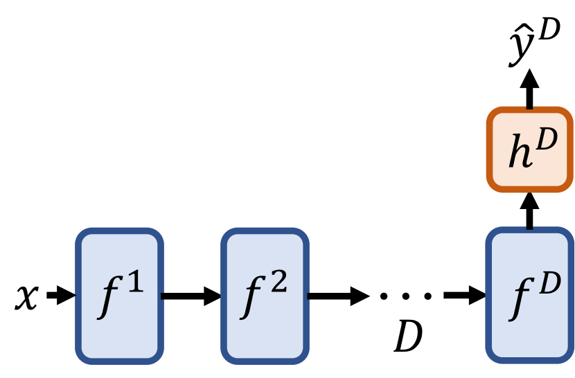
(a) Standard Single-Exit Network.

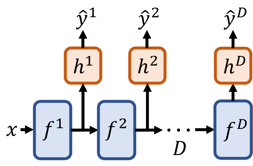
(b) Early-Exit (EE) Network.

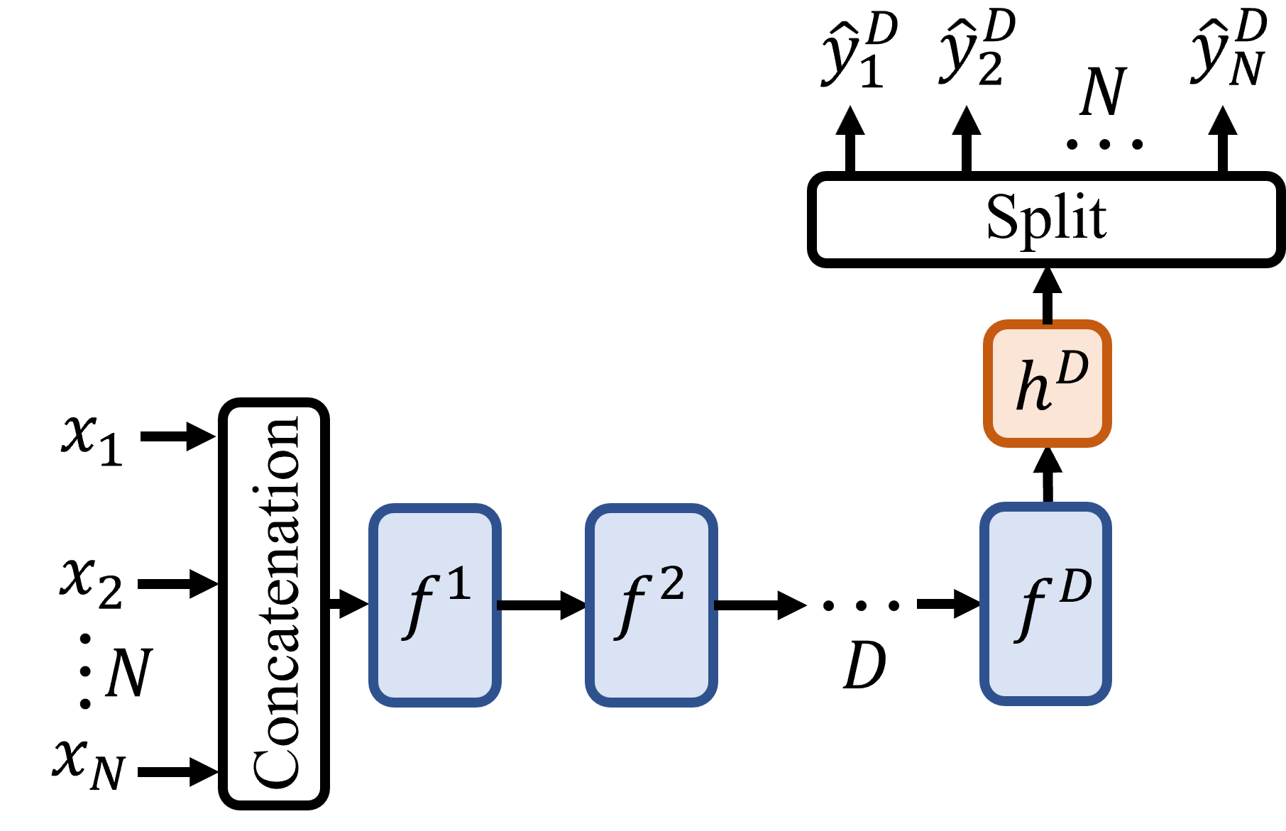
(c) Multi-Input Multi-Output (MIMO) Network.

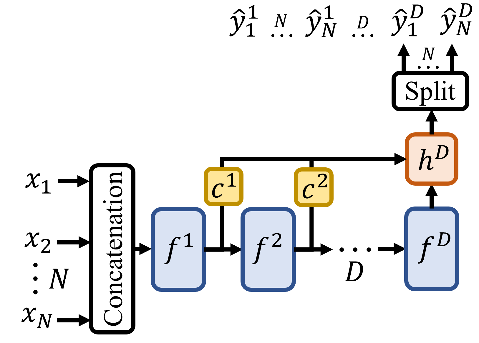
(d) Multi-Input Massive Multi-Output (MIMMO) Network.

Figure 1: Different NN architecture approaches. The filled rectangles are learnable layers $\{f^{i}(\cdot)\}^{D}_{i=1}$, prediction heads $\{h^{i}(\cdot)\}^{D}_{i=1}$ and reshaping connectors $\{c^{i}(\cdot)\}^{D-1}_{i=1}$ while the empty rectangle is a non-parametric operation. The $D$ is the network depth, and $N$ is the number of simultaneously processed inputs. The $\{x_{i}\}_{i=1}^{N}$ is the input for $N$ inputs and $\{\hat{y}_{i}^{j}\}^{N,D}_{i,j=1}$ represent the predictions from the $D$ exits for $N$ inputs. The arrows represent the flow of information.

Early-Exit (EE)

EE networks [Antorán et al., 2020, Qendro et al., 2021, Matsubara et al., 2022, Laskaridis et al., 2021] introduce minimally-parametrised auxiliary exits $\{h^{i}(\cdot)\}^{D-1}_{i=1}$ at intermediate layers of the network, which predict the output before the final exit $h^{D}(\cdot)$ at depth $D$. The EE net trains exits $\{h^{i}(\cdot)\}^{D}_{i=1}$ to jointly predict the target $y$ for a single input $x$. The EE network leverages models of varying capacity by ensembling the exits’ predictions at different network depths. At test time, the exits’ predictions $\mathbf{\hat{y}}=\{\hat{y}^{i}\}^{D}_{i=1}$ for a single input are averaged to obtain the final prediction $\hat{y}_{F}=\frac{1}{D}\sum_{i=1}^{D}\hat{y}^{i}$. The EE net is in Figure 1(b).

Multi-Input Multi-Output (MIMO)

MIMO networks [Li and Liang, 2018, Havasi et al., 2020] process multiple inputs in a single architecture while being competitive with rank-1 Bayesian NNs and BatchEnsemble approaches [Wen et al., 2020, Dusenberry et al., 2020, Wenzel et al., 2020], without having to implement custom operations. Recent work on MIMO includes feature regularisation [Soflaei et al., 2020], data multiplexing [Murahari et al., 2022] and augmentation [Ramé et al., 2021, Sun et al., 2022b, a]. A MIMO network processes inputs $\mathbf{x}=\{x_{i}\}^{N}_{i=1}$ and outputs $\mathbf{\hat{y}}=\{\hat{y}_{i}\}^{N}_{i=1}$ predictions using a single $\mathcal{F}(\cdot)$. The inputs are concatenated before the first layer, resulting in a tensor of shape $[B,N\times C,H,W]$, where $B$ is the batch size, $C$ is the number of channels, $H$ is height, and $W$ is width for e.g. image data. Except for the first layer $f^{1}(\cdot)$ with increased input size $N\times C$, the hidden layers $\{f^{i}(\cdot)\}^{D}_{i=2}$ are the same as a standard NN. The outputs are split at the end into a tensor of shape $[B,N,O]$, where $O$ are the output nodes. The MIMO net matches the individual predictions $\mathbf{\hat{y}}=\{\hat{y}_{i}\}^{N}_{i=1}$ to the distinct targets $\mathbf{y}=\{y_{i}\}^{N}_{i=1}$ during training. At test time, the predictions for repeated identical inputs $\mathbf{x}^{*}=\{x_{i}\}^{N}_{i=1}$ are averaged as $\hat{y}_{F}=\frac{1}{N}\sum_{i=1}^{N}\hat{y}_{i}$. The MIMO is visualised in Figure 1(c).

Multi-Input Massive Multi-Output (MIMMO)

A MIMMO network [Ferianc and Rodrigues, 2023] combines MIMO and EE by adding $\{h^{i}(\cdot)\}^{D-1}_{i=1}$ auxiliary prediction heads and processing $N$ inputs and outputs for each exit, resulting in $\mathbf{\hat{y}}=\{\hat{y}_{i}^{j}\}^{N,D}_{i,j=1}$ outputs. The MIMMO net trains to match the predictions between all exits $\mathbf{\hat{y}}$ and targets $\mathbf{y}=\{y_{i}^{j}\}^{N,D}_{i,j=1}$. Targets are replicated for each input $\mathbf{x}=\{x_{i}\}^{N}_{i=1}$ across $D$ to get $\mathbf{y}$. At test time, predictions are averaged as $\hat{y}_{F}=\frac{1}{N}\sum_{i,j=1}^{N,D}\hat{y}_{i}^{j}\theta_{i}^{j}$ for repeated inputs $\mathbf{x}^{*}=\{x_{i}\}^{N}_{i=1}$ where $\theta_{i}^{j}$ is the weight of exit $j$ for input $i$. MIMMO uses separate reshaping connectors $\{c^{i}(\cdot)\}^{D-1}_{i=1}$ to connect the layers $\{f^{i}(\cdot)\}^{D-1}_{i=1}$ to a single prediction head $h^{D}(\cdot)$. MIMMO is visualised in Figure 1(d).

3 SINGLE ARCHITECTURE ENSEMBLE

Figure 1 reveals previously unexplored similarities between single exit NN, EE, MIMO, and MIMMO. For instance, MIMO processes $N$ inputs and gives $N$ matching predictions. In contrast, EE and MIMMO process $1$ and $N$ inputs, producing $D$ and $N\times D$ diverse predictions within a single NN with depth $D$, respectively. Considering the complete search space between these methods based on $N$ and $D$, there are ${(2^{D}-1)}^{N}$ possible configurations – ${(2^{D}-1)}$ exits turned on or off, with at least one exit on, for each input in $N$, making selecting the optimal configuration challenging. We propose to unify the approaches and their in-between combinations from Figure 1 into the SAE framework, which enables the practitioner to explore a search space $N\times D\ll{(2^{D}-1)}^{N}$ efficiently by setting $N\geq 1$ and the maximum number of exits for each input within $N$ as $1\leq K\leq D$. The base network model is depicted in Figure 2. The network processes $N$ inputs via a widened input layer, after which the refined features of the $D$ layers are processed by exits at different depths. The framework learns the exit weighting for all $N$ inputs and their $K$ exits, enabling the NN to learn which part of the network to use as a feature extractor and which exits to use per input in $N$, giving $N\times K$ predictions. In summary, SAE maximally exploits the network’s capacity by jointly exploring the search space of the generalised methods and their in-between configurations via $N$ and $K$. It requires marginal computational overhead by introducing the widened input and the active exits during evaluation and a single training round. Next, we define the objective function, enabling us to learn the optimal depth of the exits and the network weights.

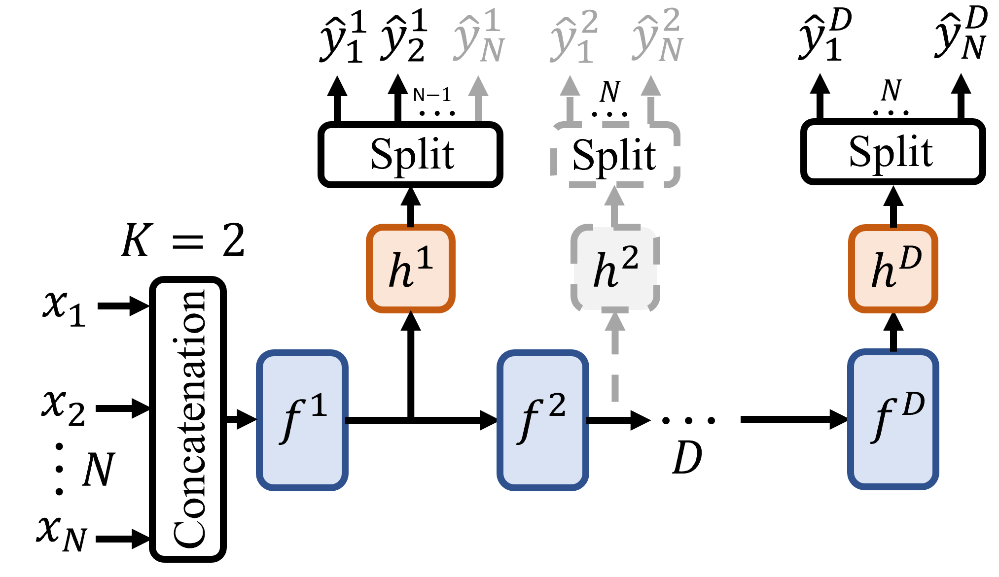
Figure 2: The Single Architecture Ensemble (SAE) Network. The filled rectangles stand for learnable layers $\{f^{i}(\cdot)\}^{D}_{i=1}$ and prediction heads $\{h^{i}(\cdot)\}^{D}_{i=1}$, while the empty rectangle represents a non-parametric operation. The $D$ is the network depth, $N$ is the number of separate inputs in the ensemble, and $K$ is the maximum number of active exits during evaluation for each input. The $\{x_{i}\}_{i=1}^{N}$ are the $N$ inputs and $\{\hat{y}_{i}^{j}\}^{N,D}_{i,j=1}$ represent the predictions from the $D$ exits for $N$ inputs. The arrows represent the flow of information. The dashed and greyed boxes and arrows represent exits that were active during training but inactive during evaluation because of top $K$ exits identified during training.

3.1 Training of SAE

We define the SAE’s training objective, initially considering $N$ independent ensemble inputs. Denote the dataset $\mathcal{D}=\{x_{i},y_{i}\}_{i=1}^{|\mathcal{D}|}$, where $x_{i}$ is the input and $y_{i}$ is the ground truth for input $i$ and $|\mathcal{D}|$ is the size of the dataset $\mathcal{D}$. We assume initially that our model processes $N$ inputs $\{x_{i}\}^{N}_{i=1}$ and produces $N$ matching outputs $\{\hat{y}_{i}\}^{N}_{i=1}$. During training, we assume that the $N$ inputs $\{x_{i}\}^{N}_{i=1}$ and targets $\{y_{i}\}^{N}_{i=1}$ are sampled independently from the dataset $\mathcal{D}$ in $N$, hence assuming independence between $p(\{y_{i}\}^{N}_{i=1}|\{x_{i}\}^{N}_{i=1},\mathbf{w})=\prod_{i=1}^{N}p(y_{i}|\{x_{z}\}^{N}_{z=1},\mathbf{w})$ [Havasi et al., 2020], where $\mathbf{w}$ are the learnable weights of the network $\mathcal{F}(\cdot)$. We denote $\mathbf{x}_{i}=\{x_{z}\}^{N}_{z=1}$ as the input for $i$, containing $x_{i}$ and $N-1$ random sampled inputs from the dataset $\mathcal{D}$, matching the $\{y_{i}\}^{N-1}_{i=1}$.

With the independence assumption, we introduce the exits, which enable the NN to make a prediction for each input $i$ at $D$ different depths as $\hat{y}_{i}^{j}=p(y_{i}|\mathbf{x}_{i},d_{i}=j,\mathbf{w})=h^{j}(f^{j}(f^{j-1}(\dots f^{1}(\mathbf{x}_{i}))))$ where $1\leq j\leq D$ and $d_{i}$ is the latent variable for $D$ exits for input $i$. The marginal likelihood or evidence of the data is $p(y_{i}|\mathbf{x}_{i},\mathbf{w})=\sum_{j=1}^{D}p(y_{i}|\mathbf{x}_{i},d_{i}=j,\mathbf{w})p(d_{i}=j)$ for a categorical prior $p(d_{i})$ where $p(d)=\prod_{i=1}^{N}p(d_{i})$. We introduce a categorical variational distribution $q(d|\mathbf{\theta})=\prod_{i=1}^{N}q(d_{i}|\mathbf{\theta}_{i})$ with parameters $\mathbf{\theta}=\{\theta_{i}^{j}\}^{N,D}_{i,j=1}$, where $\theta_{i}$ are the parameters of the weightings of all the exits for input $i$.  Antorán et al. [2020] demonstrated for $N=1$ that by choosing the prior and the variational distribution to be categorical, it is possible to jointly optimise $\mathbf{w}$ and $\mathbf{\theta}$ and maximise the evidence lower bound of the data via stochastic gradient ascent. To derive the evidence lower bound for all $N$ independent predictors, we minimise the Kulback-Leibler (KL) divergence [Csiszár, 1975] between the variational distribution $q(d|\mathbf{\theta})$ and the posterior distribution $p(d|\mathcal{D},\mathbf{w})=\prod_{i=1}^{N}p(d_{i}|\mathcal{D},\mathbf{w})$ as:

$$KL(q(d|\mathbf{\theta})\,||\,p(d|\mathcal{D},\mathbf{w}))=\sum_{i=1}^{N}KL(q(d_{i}|\mathbf{\theta}_{i})\,||\,p(d_{i}|\mathcal{D},\mathbf{w}))$$

$$= \sum_{i=1}^{N}\mathbb{E}_{q(d_{i}|\mathbf{\theta}_{i})}\left[\log q(d_{i}|\mathbf{\theta}_{i})-\log\frac{p(Y_{i}|\mathbf{X}_{i},d_{i},\mathbf{w})p(d_{i})}{p(Y_{i}|\mathbf{X}_{i},\mathbf{w})}\right]$$

$$=\underbrace{\sum_{i=1}^{N}\mathbb{E}_{q(d_{i}|\mathbf{\theta}_{i})}\left[-\log p(Y_{i}|\mathbf{X}_{i},d_{i},\mathbf{w})\right]}_{\text{Data-fit in }-\mathcal{L}(\mathbf{w},\mathbf{\theta})}$$

$$+\underbrace{KL(q(d_{i}|\mathbf{\theta}_{i})\,||\,p(d_{i}))}_{\text{Regulariser in }-\mathcal{L}(\mathbf{w},\mathbf{\theta})}+\underbrace{\sum_{i=1}^{N}\log p(Y_{i}|\mathbf{X}_{i},\mathbf{w})}_{\text{Evidence}}$$ (1)

The KL divergence in Equation 1 is decomposed into the expectation of the log-likelihood, or the data-fit term, of the data $Y_{i}=\{y_{i}^{(j)}\}^{|D|}_{j=1}$, given input tuples $\mathbf{X}_{i}=\{\mathbf{x}_{i}^{(j)}\}^{|D|}_{j=1}$ for dataset size $|\mathcal{D}|$, the exits $d_{i}$ and the weights $\mathbf{w}$, the KL divergence between the variational distribution $q(d_{i}|\mathbf{\theta}_{i})$ and the prior distribution $p(d_{i})$, or the regulariser term, and the evidence of the data. The KL divergence is non-negative, and the evidence of the data is maximised when the $\mathcal{L}(\mathbf{w},\mathbf{\theta})$ is maximised as $\mathcal{L}(\mathbf{w},\mathbf{\theta})\leq\sum_{i=1}^{N}\log p(Y_{i}|\mathbf{X}_{i},\mathbf{w})$.

The objective $\mathcal{L}(\mathbf{w},\mathbf{\theta})$ can be further decomposed with respect to all the inputs $N$ and the whole dataset $\mathcal{D}$ as in Equation 2. The $b$ is the index of the input tuple $\mathbf{x}_{i}^{(b)}$ and the target $y_{i}^{(b)}$ sampled from the dataset $\mathcal{D}$. We assume a uniform categorical prior, meaning that the KL divergence between the variational distribution $q(d|\mathbf{\theta})$ and the prior distribution $p(d)$ can be computed in closed form.

$$\mathcal{L}(\mathbf{w},\mathbf{\theta}) =\sum_{i=1}^{N}\mathbb{E}_{q(d_{i}|\mathbf{\theta}_{i})}\left[\log p(Y_{i}|\mathbf{X}_{i},d_{i},\mathbf{w})\right]$$

$$-\sum_{i,j=1}^{N,D}\theta_{i}^{j}\log\frac{\theta_{i}^{j}}{D^{-1}}$$

$$=\sum_{i,b=1}^{N,|\mathcal{D}|}\mathbb{E}_{q(d_{i}|\mathbf{\theta}_{i})}\left[\log p(y_{i}^{(b)}|\mathbf{x}_{i}^{(b)},d_{i},\mathbf{w})\right]$$

$$-\sum_{i,j=1}^{N,D}\theta_{i}^{j}\log\frac{\theta_{i}^{j}}{D^{-1}}$$ (2)

Equation 3 approximates the evidence lower bound, where $B$ is the batch size.

$$\mathcal{L}(\mathbf{w},\mathbf{\theta}) \approx\frac{|\mathcal{D}|}{B}\sum_{i,b=1}^{N,B}\mathbb{E}_{q(d_{i}|\mathbf{\theta}_{i})}\left[\log p(y_{i}^{(b)}|\mathbf{x}_{i}^{(b)},d_{i},\mathbf{w})\right]$$

$$-\sum_{i,j=1}^{N,D}\theta_{i}^{j}\log\frac{\theta_{i}^{j}}{D^{-1}}$$ (3)

We propose to sample the depth variable $d_{i}$ from the variational distribution $q(d_{i}|\mathbf{\theta}_{i})$ using a top $K$ sampling strategy [Kool et al., 2019] which enables us to optimise the $\mathbf{\theta}$ towards the top $K$ exits per input. We use one Monte Carlo sample per batch to approximate the expectation, the sum of the $D$ log-likelihoods multiplied by the sampled probabilities of $d_{i}$. The $\mathbf{\theta}$ are practically implemented as zero-initialised logits divided by a temperature $T$ to which softmax was applied to normalise the logits to sum to 1 as $\theta_{i}^{j}=\frac{\exp(l_{i}^{j}/T)}{\sum_{k=1}^{D}\exp(l_{i}^{k}/T)}$ and $l_{i}^{j}$ is the $j$-th exit logit for input $i$. In summary, the training objective $\mathcal{L}(\mathbf{w},\mathbf{\theta})$ allows us to learn the exit preferences $\mathbf{\theta}$ for each input $i\in N$ and each exit $j\in D$ along the network’s weights $\mathbf{w}$ via gradient ascent, given the architecture and the dataset.

3.2 Training Scheduling Regularisation

During experimentation, we observed that the training of the SAE might be compromised by overregularisation, which can be caused by the regulariser term in Equation 3 or by the size of the dataset $|\mathcal{D}|$. We introduce a $\alpha(t)$ factor to enable the trade-off between fitting the data and regularisation to give the final loss function in Equation 4.

$$\mathcal{L}(\mathbf{w},\mathbf{\theta}) =\frac{1}{B}\sum_{i,b=1}^{N,B}\mathbb{E}_{q(d_{i}|\mathbf{\theta}_{i})}\left[\log p(y_{i}^{(b)}|\mathbf{x}_{i}^{(b)},d_{i},\mathbf{w})\right]$$

$$-\alpha(t)\sum_{i,j=1}^{N,D}\theta_{i}^{j}\log\frac{\theta_{i}^{j}}{D^{-1}}$$ (4)

The weight $0\leq\alpha(t)\leq 1$ is a linear interpolation depending on the training step $t$. The starting and ending values of $\alpha(t)$ can be optimised. Similarly, we propose to linearly interpolate between starting and ending values of the temperature $0<T(t)\leq 1$, where the starting and ending values can again be optimised. Therefore, during sampling, the probabilities over the auxiliary exits can be made sharper over time, which enables the framework to gradually focus on the $K$ most important auxiliary exits for each input in the architecture. To enable feature reuse in the architecture, we propose linearly interpolating the input repetition factor $0\leq r(t)\leq 1$, where the starting and ending values can be optimised. The $r(t)$ determines a portion of the batch $B$ where the same input is repeated across all the $N$ inputs, relaxing the independence assumption [Havasi et al., 2020]. In summary, the interpolation of hyperparameters aims to enable the framework to iterate over multiple hyperparameter settings during training, which targets the challenge of finding the optimal hyperparameters for the generalised methods and the SAE framework.

3.3 Evaluation of SAE

During the evaluation, the SAE framework produces $N\times K$ predictions $\{\hat{y}_{i}^{j}\}^{N,K}_{i,j=1}$, where $K$ is the number of exits used for each input in $N$. It does so through only keeping the top $K$ logits and setting the rest to negative infinity to give $\mathbf{\theta}^{*}=\{\theta_{i}^{*j}\}^{N,K}_{i,j=1}$. Similarly, the top $K$ exits are initialised to give network $\mathcal{F}^{*}(\cdot)$. If no inputs select an exit at some level $j$, it does not need to be implemented as shown in Figure 2 in grey. The input sample is repeated $N$ times as $\mathbf{x}^{*}=\{x_{i}\}^{N}_{i=1}$ and the predictions from the active exits are collected. The final prediction is obtained by averaging the predictions from the exits and their $\theta_{i}^{*j}$ as $\hat{y}_{F}=\frac{1}{N}\sum_{i,j=1}^{N,K}\hat{y}_{i}^{j}\theta_{i}^{*j}$ which approximates the marginal likelihood. The training and evaluation of the SAE framework are summarised in Algorithm 1. The SAE training operates over a fixed number of steps $t_{end}$. For each step, it iterates over a batch size $B$, $\mathbf{x}^{(b)}=\{\mathbf{x}_{i}^{(b)}\}^{N}_{i=1}$ and $\mathbf{y}^{(b)}=\{y_{i}^{(b)}\}^{N}_{i=1}$, sampled from the dataset $\mathcal{D}$ according to the input repetition factor $r(t)$ and $N$. It then computes predictions $\{\hat{y}_{i}^{j,(b)}\}^{N,D}_{i,j=1}$ using the current model and samples the depth variables from a distribution $q(d|\mathbf{\theta})$ for all $N$. Using these predictions and the sampled depth variables, the loss $\mathcal{L}(\mathbf{w},\mathbf{\theta})$ is calculated, and $\mathbf{w},\mathbf{\theta}$ are updated through backpropagation. The evaluation involves retaining the top $K$ parameters of $\mathbf{\theta}$ while setting the rest of the logits to negative infinity. It repeats input $\mathbf{x}^{*}=\{x_{i}\}^{N}_{i=1}$ $N$ times and computes the prediction $\hat{y}_{F}$.

Algorithm 1 Single Architecture Ensemble (SAE)

1:procedure Train($\mathcal{D}$,$\mathbf{w}$,$\mathbf{\theta}$,$B$,$N$,$D$,$K$,$\alpha(t)$,$T(t)$,$r(t)$, $t_{end}$)

2:     for $t=1$ to $t_{end}$ do

3:         for $b=1$ to $B$ do

4:              Sample $\mathbf{x}^{(b)}$, $\mathbf{y}^{(b)}$ from $\mathcal{D}$ at batch index $b$ with respect to input repetition factor $r(t)$ and $N$

5:              Predict $\{\hat{y}_{i}^{j,(b)}\}^{N,D}_{i,j=1}=\mathcal{F}(\mathbf{x}^{(b)},\mathbf{w})$

6:         end for

7:         Sample $\{d_{i}\}_{i=1}^{N}$

8:         Compute $\mathcal{L}(\mathbf{w},\mathbf{\theta})$ using Equation 4

9:         Backpropagate and update $\mathbf{w}$, $\mathbf{\theta}$

10:     end for

11:end procedure

12:procedure Evaluate($\mathcal{D}$,$\mathbf{w}$,$\mathbf{\theta}$,$N$,$D$,$K$,$T(t_{end})$)

13:     Keep top $K$ $\mathbf{\theta}^{*}$ and set the rest to -inf for all $i\in N$; initialise top $K$ active exits for $\mathcal{F}^{*}(\cdot)$

14:     Repeat input $\mathbf{x}^{*}=\{x_{i}\}^{N}_{i=1}$ $N$ times

15:     Predict $\{\hat{y}_{i}^{j}\}^{N,K}_{i,j=1}=\mathcal{F}^{*}(\mathbf{x}^{*},\mathbf{w})$

16:     Predict $\hat{y}_{F}=\frac{1}{N}\sum_{i,j=1}^{N,K}\hat{y}_{i}^{j}\theta_{i}^{*j}$

17:end procedure

3.4 RELATIONSHIP TO GENERALISED METHODS

SAE unifies single exit (SE) NN, EE, MIMO, and MIMMO approaches into a single framework through the combination of $N$ and $K$ parameters for a network of depth $D$ as follows:

• if $N=1$ and $K=1$ this is a SE NN;

• if $N=1$ and $K\geq 2$, this is an EE network;

• if $N\geq 2$ and $K=1$, this is a MIMO network;

• if $N\geq 2$ and $K=D$, this is a MIMMO network.

A distinctive feature of SAE is its ability to determine the most effective exit depth for each input, a capability previously investigated in SE NN, EE and MIMMO [Antorán et al., 2020, Ferianc and Rodrigues, 2023], but not in MIMO. MIMMO, where $N\geq 2$ and $K=D$, is the closest approach to SAE. It also learns the exit depth for each input but uses all the exits during evaluation. As empirically observed, small capacity NNs might not have enough capacity to make meaningful predictions at all depths, hence the need for the $K$ parameter. Additionally, SAE diverges from the MIMMO by not adopting a common prediction head across all exits, which we empirically found to degrade performance. Moreover, SAE introduced HP scheduling, which was not considered in MIMMO. In essence, SAE’s objective is not to rival the generalised methods but to amalgamate them into a cohesive framework facilitated by setting $N$ and $K$. Next, we show that various problems, including hybrid solutions, require different methods.

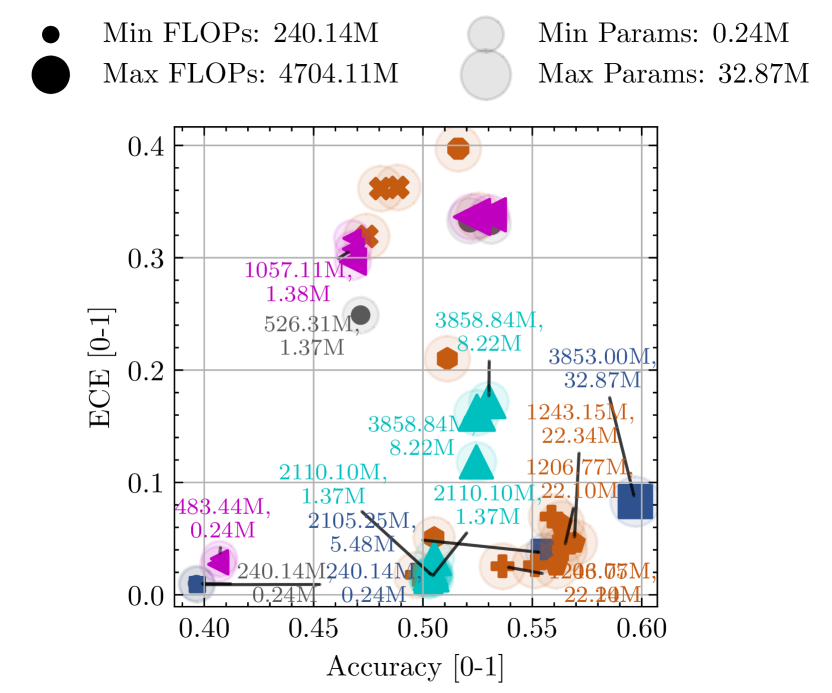
(a) TinyImageNet ID.

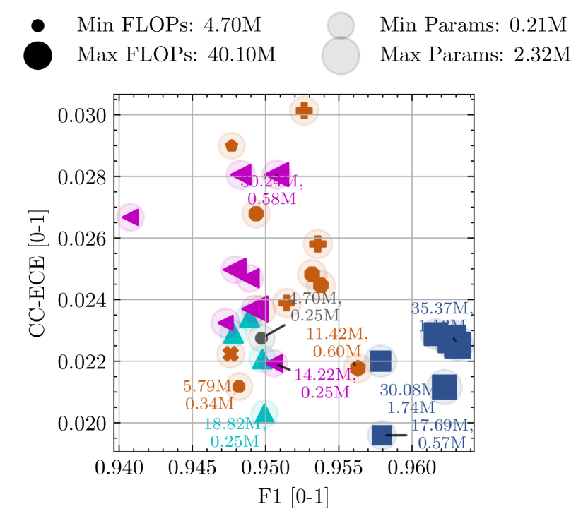
(b) BloodMNIST ID.

(c) PneumoniaMNIST ID.

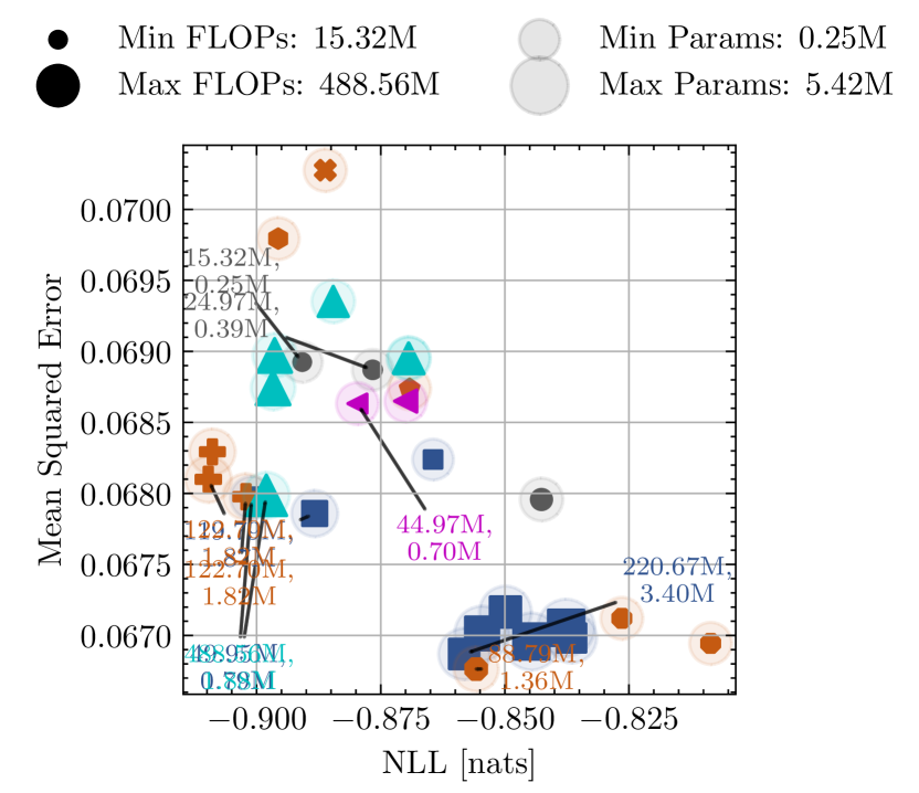
(d) RetinaMNIST ID.

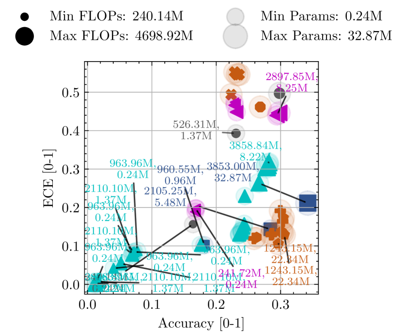
(e) TinyImageNet OOD.

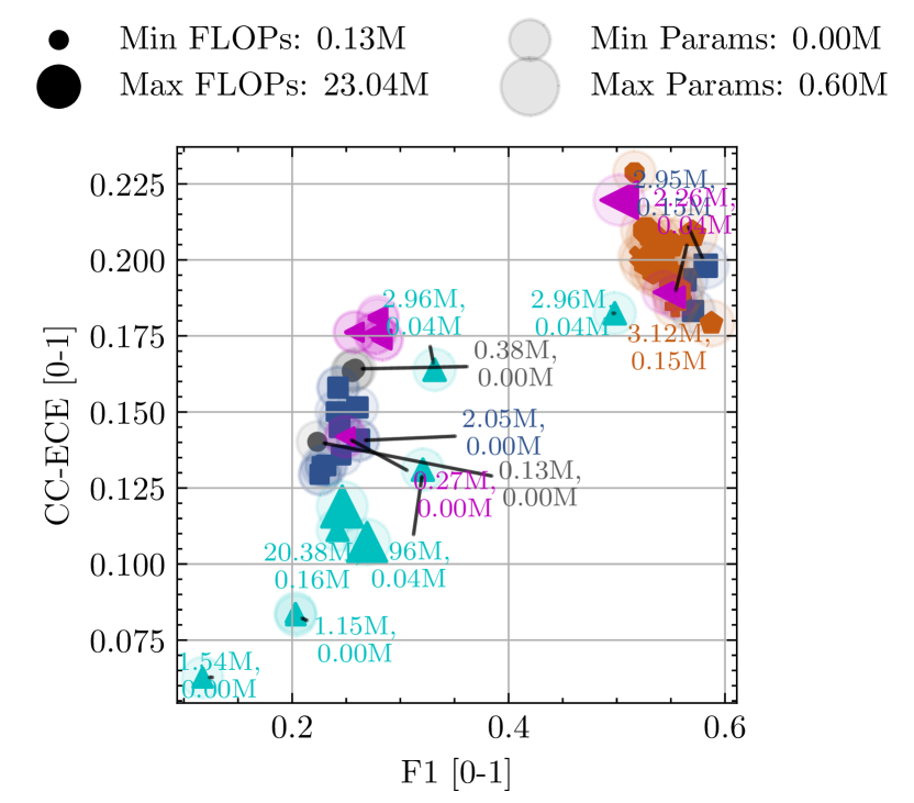
(f) BloodMNIST OOD.

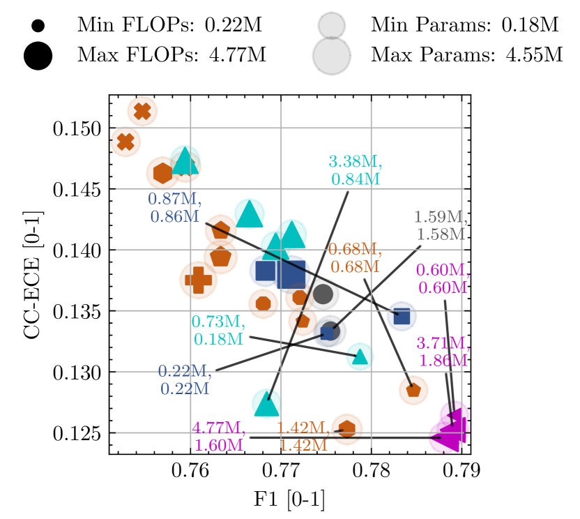
(g) PneumoniaMNIST OOD.

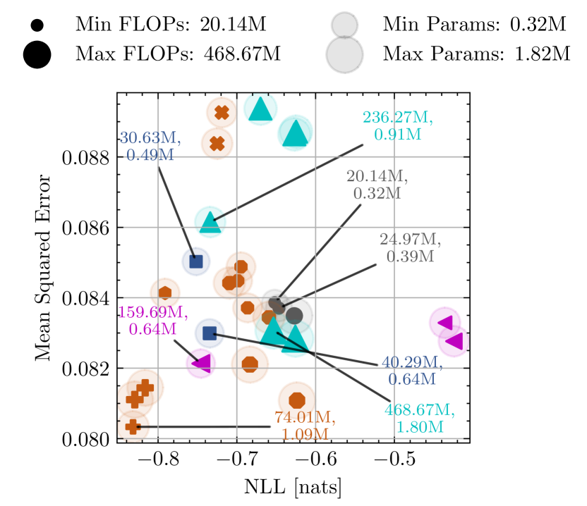
(h) RetinaMNIST OOD.

Figure 3: Comparison on TinyImageNet, BloodMNIST, PneumoniaMNIST, and RetinaMNIST across ID (upper row) and OOD (lower row) datasets, with respect to Standard NN $\newmoon$, NN Ensemble $\blacksquare$, SAE: I/B: $N\geq 2,2\leq K<D$ , EE: $N=1,K\geq 2$ , MIMMO: $N\geq 2,K=D$ , MIMO: $N\geq 2,K=1$ , SE NN: $N=1,K=1$ , MCD $\blacktriangle$, BE $\blacktriangleleft$. The size of the marker denotes the number of FLOPs, and the shaded region denotes the number of parameters. The first row of the caption denotes the number of FLOPs, and the second row denotes the number of parameters.

4 EXPERIMENTS

We perform experiments on four datasets: TinyImageNet [Le and Yang, 2015], BloodMNIST, PneumoniaMNIST and RetinaMNIST, [Yang et al., 2023] for both classification and regression tasks. Our architecture backbones are ResNet for TinyImageNet, ViT for RetinaMNIST, VGG for BloodMNIST, and a residual fully connected net with batch normalisation and ReLU activations (FC) for PneumoniaMNIST. We compare approaches under SAE with Monte Carlo Dropout (MCD) [Gal and Ghahramani, 2016], where we insert dropout layers before each linear or convolutional layer. We also compare to Batch Ensemble (BE) [Wen et al., 2020], where the BE layers replace all linear and convolutional layers in the network. The algorithmic lower bound is a standard NN. The algorithmic upper bound is a naive ensemble of NNs. We employ multi-objective Bayesian optimisation (MOBO) to perform hyperparameter optimisation (HPO) for SAE and: $1\leq N\leq 4,1\leq K\leq D$ the input repetition, alpha and temperature start and end values and the width of the network for all the evaluated metrics simultaneously on the validation dataset. For all the other methods, we enumerate networks of all widths, depths, or $N$ for BE and NN ensembles. An exception is MCD, for which we set $N=4$ to make it competitive. We use MOBO to search for the MCD or SAE’s parameters. We minimise unweighted negative log-likelihood (NLL) loss for all tasks except for SAE. For classification, we measure F1 score $[\uparrow 0,1]$, Accuracy $[\uparrow 0,1]$, Expected Calibration Error (ECE) $[\downarrow 0,1]$, Class Conditional ECE (CC-ECE) $[\downarrow 0,1]$ and the NLL $[\downarrow 0,\infty)$ as evaluation metrics. We use the F1 score and CC-ECE to measure the performance under unbalanced settings instead of accuracy or ECE insensitive to class imbalance. For regression, we use Gaussian NLL $[\downarrow-\infty,\infty)$ and mean squared error (MSE) $[\downarrow 0,\infty)$ as evaluation metrics. From the hardware perspective, we measure the number of floating point operations (FLOPs) $[\downarrow 0,\infty)$ and the number of parameters $[\downarrow 0,\infty)$. We test on ID and OOD data created by applying augmentations to the test set, such as Gaussian noise, motion blur, and contrast changes [Hendrycks and Dietterich, 2019]. The OOD experiments are crucial since the naive ensemble’s algorithmic confidence calibration is solid under the OOD setting [Ovadia et al., 2019], motivating their use in practice despite their high computational cost. We chose feed-forward, residual, convolutional, fully connected, or transformer architectures of various capacities, a combination of classification and regression tasks, and balanced and unbalanced datasets in RGB or grayscale, with many or few data samples across ID and OOD data to demonstrate the versatility of our framework in different applications. The Appendix details architectures, datasets, metrics, HPO runs, additional results, the minimal network modification required by SAE, a hardware cost breakdown, and a comparison to the baselines. Next, we compare the performance of SAE to the baselines, investigate if there is a default $K$ and $N$ configuration across datasets and tasks, how depth preference changes across different architectures and whether interpolation of hyperparameters is beneficial.

4.1 Baseline Comparison

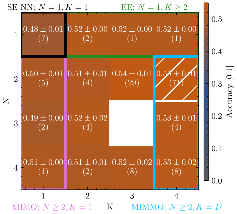
(a) Accuracy on TinyImageNet.

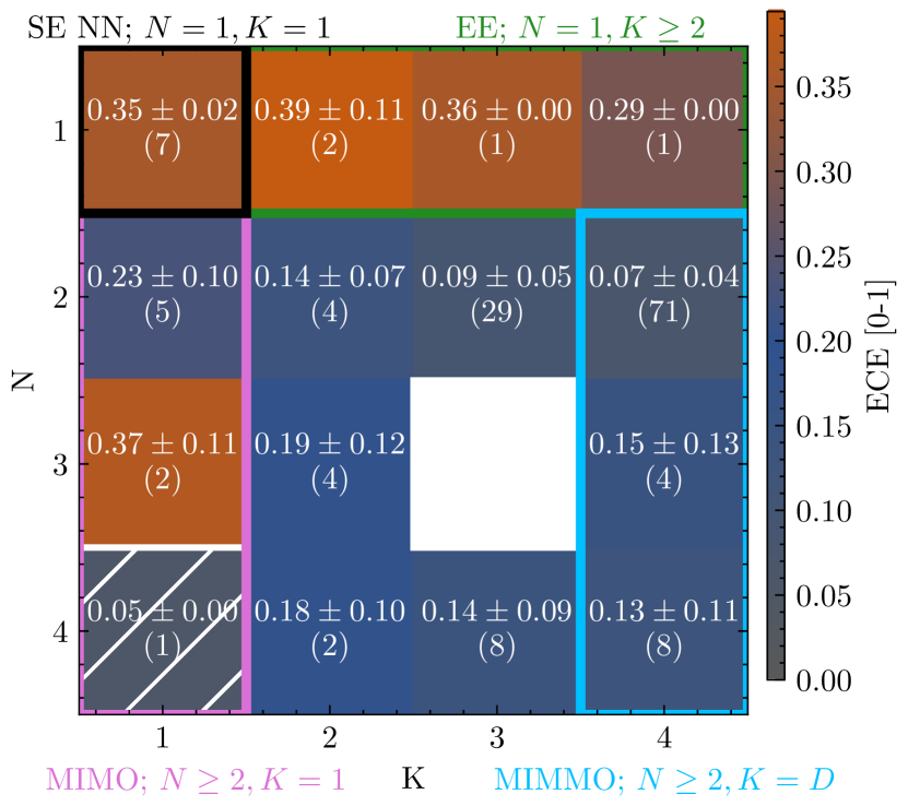
(b) ECE on TinyImageNet.

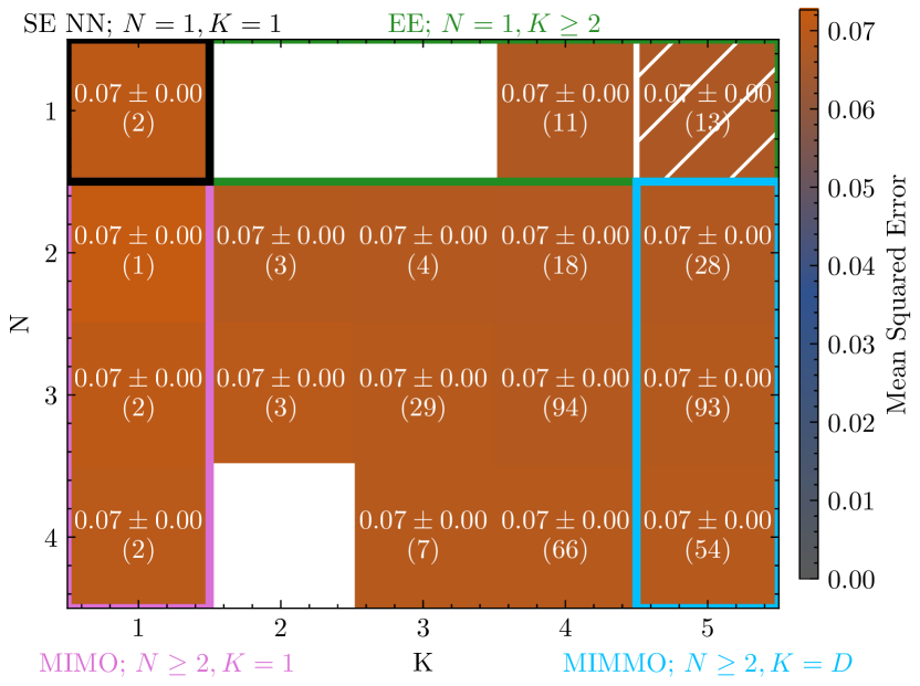
(c) MSE on RetinaMNIST.

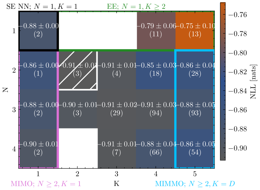
(d) NLL on RetinaMNIST.

Figure 4: Varying $N,K$ on TinyImageNet and RetinaMNIST ID test sets. The upper number is the average performance over $N$, $K$ combinations. The number in brackets is the number of sampled configurations by HPO. White box means no configurations sampled for that $N$, $K$. Pattern signals best average performance. The coloured outlines signal the special cases for the generalised methods.

In Figure 3, we compare Pareto optimal configurations identified via HPO across all metrics and datasets. In the upper row, we show the results on the ID test set, and in the lower row, we demonstrate the results on the OOD test set created through augmentations. The size of the marker denotes the number of FLOPs, and the shaded region denotes the number of parameters; some of the points are commented with concrete values. Note the min/max ranges for FLOPs and a number of parameters, signifying models of various capacities. We split the methods in SAE into 5 categories based on the $N$ and $K$ values: I/B: $N\geq 2,2\leq K<D$ , EE: $N=1,K\geq 2$ , MIMMO: $N\geq 2,K=D$ , MIMO: $N\geq 2,K=1$ , SE NN: $N=1,K=1$ . We denote I/B as the in-between configuration across the generalised methods. The results are averaged across 4 runs with different random seeds. The Appendix contains numerical results for each metric, the dataset’s best configurations, and NLL comparison. For TinyImageNet, in Figures 3(a) and 3(e), it can be seen that the ensemble $\blacksquare$ achieves the best accuracy on ID and OOD data. However, SAE can find I/B configuration within 3% of accuracy, but 4% better ECE and significantly lower NLL than the best ensemble $\blacksquare$ with $3.2\times$ fewer FLOPs and $1.5\times$ fewer parameters. On OOD data, the same I/B configuration is within the standard deviation of accuracy and with better mean ECE and NLL than the best ensemble $\blacksquare$ while conserving the same FLOPs and parameters. For BloodMNIST, in Figures 3(b) and 3(f), it can be seen that the ensemble $\blacksquare$ achieves the best algorithmic performance on ID data. At the same time, the SAE can find an MIMO configuration which is within 1% of the F1 score or CC-ECE with a comparable number of parameters but approximately $1.5\times$ fewer FLOPs. On OOD data, the SAE configurations all achieve high F1 score in comparison to the baselines, and a I/B configuration is within 2% of CC-ECE or F1 of the best ensemble $\blacksquare$ with $2.7\times$ fewer FLOPs and $3.7\times$ fewer parameters. For PneumoniaMNIST, in Figures 3(c) and 3(g), it can be seen that in terms of F1 score and CC-ECE on ID data, an EE configuration is the best-performing method with approximately half FLOPs than closest BE $\blacktriangleleft$. On OOD data, SAE can find a MIMMO configuration which is within 1% of the best BE $\blacktriangleleft$ with similar FLOPs and parameters. For RetinaMNIST, in Figure 3(d) and 3(h), it can be seen that in terms of NLL the MIMO configuration is comparable to the ensemble $\blacksquare$ with marginally fewer FLOPs and parameters. On OOD data, the I/B configuration is the best-performing method with approximately $2\times$ fewer FLOPs than the second best BE $\blacktriangleleft$. In summary, SAE can find a set of competitive or better configurations than the baselines across all datasets, tasks, architectures with various capacities, and evaluation metrics using fewer or comparable FLOPs and parameters. In particular, SAE often achieves the best confidence calibration across ID or OOD data, measured via ECE, CC-ECE, or NLL. This motivates replacing the naive ensemble with SAE in practice. SAE does not need custom operations as in BE, random number generators as in MCD, or more training rounds than a standard NN, MCD, or BE. SAE only needs to add compute-efficient early exits and an enlarged input layer capable of processing multiple inputs simultaneously, as detailed in the Appendix.

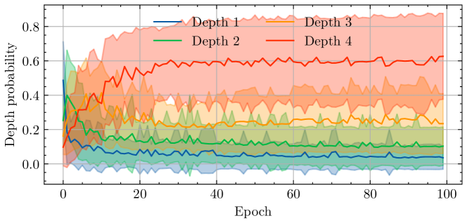
(a) TinyImageNet.

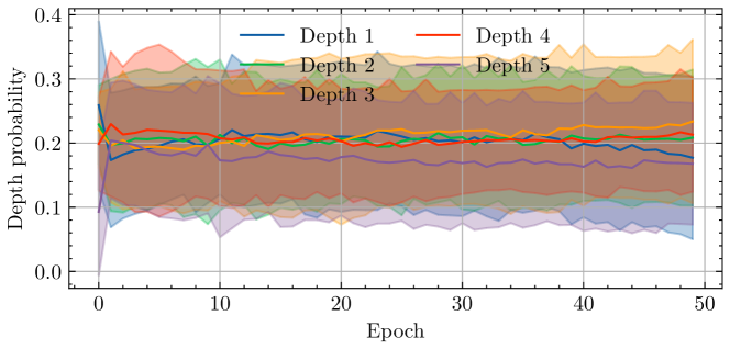
(b) RetinaMNIST.

Figure 5: Depth preference during training for TinyImageNet and RetinaMNIST. The lines denote the mean trend, and the shaded regions denote the standard deviation across all $N$ and $K$ combinations.

4.2 Changing K and N

This experiment investigates the average performance across $K$ and $N$ across the HPO runs for TinyImageNet – ResNet and RetinaMNIST – ViT. Other datasets are shown in the Appendix. The results are visualised in Figure 4. The box outlines denote the generalised methods. For example, TinyImageNet’s accuracy and ECE are improved when considering $N\geq 2$ and $K\geq 2$, while RetinaMNIST’s MSE and NLL are improved when considering $N=3$ and $K\geq 2$. However, for accuracy for TinyImageNet, the best average performance is achieved when $N=2$ and $K=4$, while for ECE, the best average performance is achieved when $N=4$ and $K=1$. This differs to [Ferianc and Rodrigues, 2023, Havasi et al., 2020] where $N>1$ consistently leads to worse algorithmic performance. As the Figure shows, different combinations of $N$ and $K$ achieve the best performance for different metrics, datasets, and architectures. This motivates our SAE framework to consider all the submethods jointly.

4.3 Depth Preference

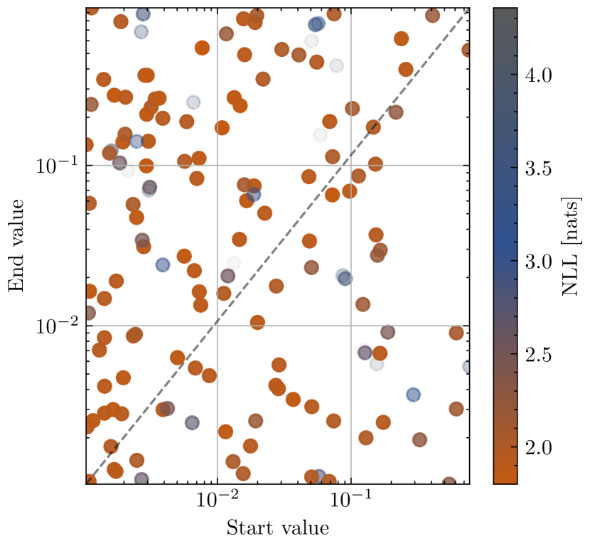
(a) Temperature for TinyImageNet.

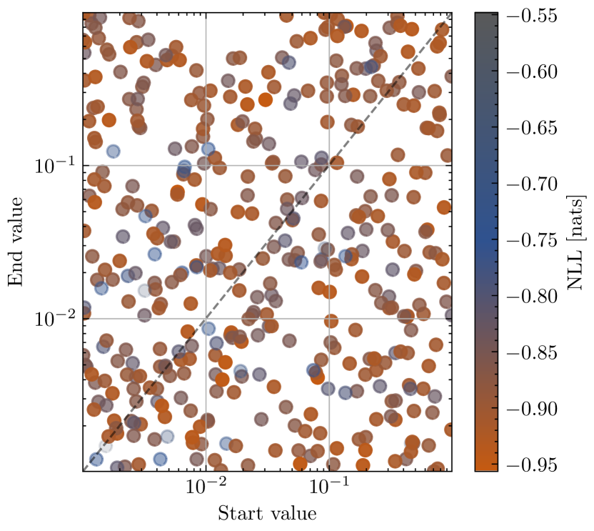
(b) Temperature for RetinaMNIST.

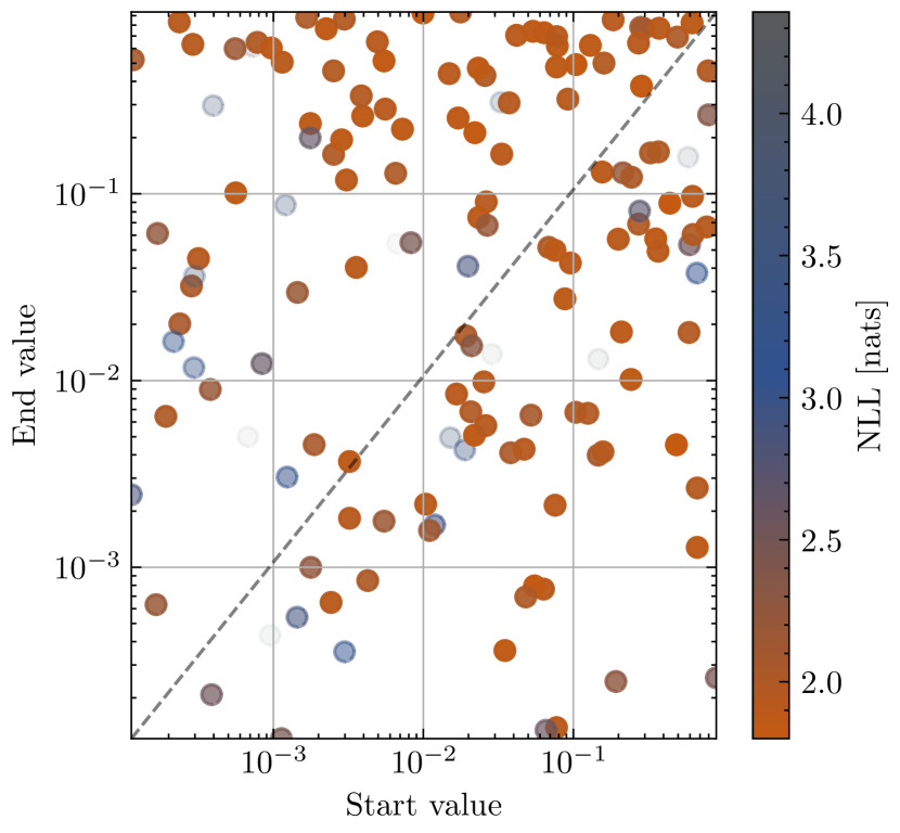
(c) Alpha for TinyImageNet.

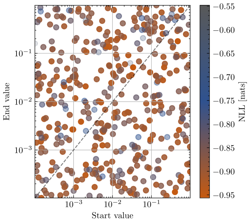
(d) Alpha for RetinaMNIST.

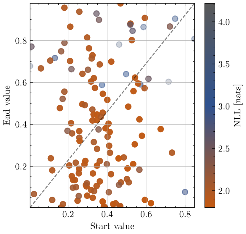
(e) Input repetition probability for TinyImageNet.

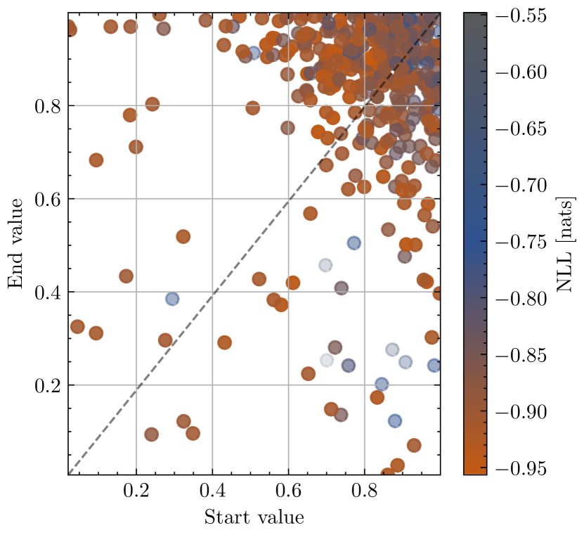
(f) Input repetition probability for RetinaMNIST.

Figure 6: HP tuning for TinyImageNet and RetinaMNIST NLL on the ID test set.

In this experiment, we investigate how the depth preference changes during training for TinyImageNet and RetinaMNIST. Other datasets are shown in the Appendix. The results are visualised in Figure 5. The Figure shows the average depth probability across all HPO trials for different $N$ and $K$ combinations. For a convolutional architecture for TinyImageNet, the depth preference is strongly biased towards the deeper exits. In contrast, for a ViT architecture for RetinaMNIST, the depth preference is uniform across all the exits. A convolutional VGG backbone for BloodMNIST supports this result, while the FC backbone for PneumoniaMNIST is similar to the ViT backbone for RetinaMNIST. The Appendix shows that these trends are consistent for different $N$. Early exits could be arbitrarily placed in a vision transformer and a fully connected network but should be placed in the deeper layers of a convolutional architecture. In summary, these results indicate that the depth preference changes across different architectures and datasets, which motivates learning the depth preference during training.

4.4 Hyperparameter Schedules

In this experiment, we investigate the influence of temperature, alpha or input repetition probability scheduling on the performance of TinyImageNet and RetinaMNIST across all HPO runs. Other datasets are shown in the Appendix. The results are visualised in Figure 6 for NLL. The scatter plots show the start and end values, and the colour denotes the performance of the configuration; the diagonal line represents the same start and end value. As can be seen, the HPO was not focused on choosing the HPs to be equal at the start and end of the training, which would lie on a diagonal line. Also, there is no clear correlation between the start and end values and the performance of the configuration. Therefore, we claim the usefulness of the regularising schedules for alpha, temperature and the input repetition probability.

5 CONCLUSION

In this paper, we presented the Single Architecture Ensemble (SAE). This unified framework melds the strengths of diverse hardware-efficient ensemble methods, outperforming traditional baselines in confidence calibration, accuracy and versatility across varied datasets, tasks, and architectures. Our findings underscore the necessity of SAE due to the lack of a universally superior method across all datasets, tasks, and architectures. Furthermore, we showed the different requirements for different architectures and the usefulness of adaptive hyperparameter scheduling. We plan to optimise the hardware and software metrics jointly in future work.

SAE: Single Architecture Ensemble Neural Networks
(Supplementary Material)

6 EXPERIMENTAL SETUP

Our code is implemented in PyTorch. No specific hardware optimisations were used to accelerate the training or evaluation for any methods. We fixed the number of epochs to 50 for all datasets except TinyImageNet, for which we set it to 100. We use Adam optimiser, starting with a learning rate of 3e-4 and a weight decay of 1e-5, except TinyImageNet, for which we set the weight decay to 0, and cosine annealing learning rate scheduler [Loshchilov and Hutter, 2016] across all datasets. We used batch size 64 for PneumoniaMNIST and RetinaMNIST and 128 for TinyImageNet and BloodMNIST. For Batch Ensemble, we had to find a batch size close to the other experiments’ batch size and a multiple of $1\leq N\leq 4$. Therefore, for experiments where batch size 64 was used, we used 72 for Batch Ensemble, and for experiments where batch size 128 was used, we used 144 for Batch Ensemble. The batch repetition factor [Havasi et al., 2020] for SAE was set to 2, except for TinyImageNet, where we set it to 1. We used gradient clipping with a maximum norm of 5.0 to avoid exploding gradients across all experiments. We used the default PyTorch initialisation for all layers. We fixed the base HP, such as the learning rate, weight decay, batch size, and number of epochs for all methods, to the same values for fair comparison and to demonstrate the ease of implementing SAE based on existing solutions.

We used the validation data to guide the multi-objective Bayesian optimisation (MOBO) from syne-tune [Salinas et al., 2022, Paria et al., 2020] to perform HPO. We used 10% of the training data as validation data across all datasets. We enable 50 random initialisations for exploration. We used 2 GTX 1080 and 2 RTX 2080 GPUs in one machine, giving us 4 workers for the HPO. We run for 8 hours on 4 GPUs for BloodMNIST, PneumoniaMNIST, and RetinaMNIST and 8 days on 4 GPUs for TinyImageNet. For SAE we set the search space for $r_{start}(t)$ to $[0.0,1.0]$ and $r_{end}(t)$ to $[0.0,1.0]$. For $\alpha_{start}(t)$ and $\alpha_{end}(t)$ we set the search space to $[0.00001,1.0]$ on a log scale. For $T_{start}(t)$ and $T_{end}(t)$ we set the search space to $[0.001,1.0]$ on a log scale. We set the search space for the dropout rate to $[0.0,1.0]$ on a linear scale. Dropout was not added before the first layer and after the last layer in any architecture. $N=4$ Monte Carlo samples are used during evaluation for Dropout. For ViT, it was added only where dropout would usually be added in the original architecture.

For TinyImageNet, we performed experiments on a ResNet with [3,4,6,3] residual blocks per stage, strides [2,2,2,2] and channels [64,128,256,512] within which we only enabled the search for the number of inputs $N$ and a depth $D\in\{1,4\}$, in addition to the regularisation parameters. Here, depth refers to the stage depth, not the overall depth of the network. With $D=4$, this is the standard ResNet-50 architecture. For ViT and RetinaMNIST, we enable to vary the encoder depth $D\in\{1,5\}$, width multiplier for base hidden dimension 192 as $W\in\{1,4\}$, the patch size 4, 4 heads and embedding dimension 192 and no dropout enabled by default. The depth refers to the number of encoder layers in ViT. The width multiplier multiplies the base hidden dimension of the ViT encoder. For ViT, we add a token for each additional input, but we design the final layer as a pooling of all the tokens to arrive at the prediction. We empirically observed that this leads to better performance than just the added tokens for prediction. For VGG and BloodMNIST, we enable to vary $D\in\{1,5\}$ and $W\in\{1,4\}$ with base width $[4,8,16,32,32]$ per stage and $[1,1,1,1,1],[1,1,2,2,2]$ blocks per stage, we omit the repeated memory-expensive linear layers at the end of the network and replace them with a single predictive linear layer. Each block consisted of a convolutional layer, batch normalisation, and ReLU; the first three stages included a max pooling layer in the last block of each stage. The depth refers to the number of stages in VGG. The width multiplier multiplies the base width of the VGG network per stage. For FC and PneumoniaMNIST, we design a residual fully connected network where the input is processed through an initial linear layer, upscaled to the hidden dimension, and then processed through a series of residual blocks, of a linear layer, batch normalisation, ReLU, we enable to vary $D\in\{1,5\}$ and $W\in\{1,4\}$ with base width 128. The depth refers to the number of residual blocks in FC. The width multiplier multiplies the base width of the FC network. We varied the search space size from the smallest, for example, on TinyImageNet, to the largest, for instance, on BloodMNIST, to demonstrate the adaptability of SAE to different search spaces. Note that for SAE, the depth is permanently fixed to the maximum.

The classification on TinyImageNet, BloodMNIST and RetinaMNIST was performed by processing the outputs of the last layer through a softmax function. The mean over all predictions was used as the final prediction for all the methods. For regression on RetinaMNIST, one output node was used as the mean, and the second output was processed through an exponential function to obtain the variance for minimising the Gaussian negative log-likelihood per example. The mean over all predictions was computed as the mean across all the mean outputs. The variance was computed as the mean of the variances plus the variance of the means by the law of total variance.

6.1 DATASETS

We used the following datasets for our experiments:

MedMNIST

MedMNIST [Yang et al., 2023] offers diverse medical imaging tasks: binary/multi-class classification and regression in a standardised, MNIST-like format that enables benchmarking with a reasonable computational cost. Given its multi-fidelity nature covering grayscale or RGB images, class imbalance and varying number of samples in the datasets, it presents a more realistic and challenging benchmark than other clean datasets such as MNIST, FashionMNIST or CIFAR-10/100.

• PneumoniaMNIST is derived from a dataset of pediatric chest X-ray images aimed at binary classification between pneumonia and normal cases. It includes 5,856 images originally pre-processed to $28\times 28$ grayscale images.

• BloodMNIST consists of 17,092 blood cell microscope images from individuals without infection or disease, categorised into 8 classes representing different cell types. The images are RGB and originally pre-processed to $28\times 28$.

• RetinaMNIST originates from the DeepDRiD challenge, offering 1,600 retina fundus images for regression to grade diabetic retinopathy severity on a five-level scale. The images are RGB and originally pre-processed to $28\times 28$.

In pre-processing, we pad the images to 32 pixels, random cropping and normalisation are applied to the training data, and normalisation is only used for the validation and test data. For RetinaMNIST, we normalised the ordered levels of the regression target to $[0,1]$, and we modelled the prediction as parameters of a Gaussian distribution with a mean and variance output to enable us to model the uncertainty in the predictions and benchmark the negative log-likelihood.

TinyImageNet

TinyImageNet [Le and Yang, 2015] is a subset of the ImageNet dataset [Deng et al., 2009] with 200 classes and 500 images per class, resulting in 100,000 training images and 10,000 test images. Compared to MedMNIST, TinyImageNet is a more challenging dataset with higher-resolution images and more classes. However, the dataset is balanced, and the images are relatively clean. The images are RGB and pre-processed initially to $64\times 64$. In pre-processing, random cropping and normalisation are applied to the training data, and normalisation is only used for the validation and test data. For TinyImageNet, we used 10% of the training data as validation data.

We considered datasets of varying image sizes ($64\times 64$ against $28\times 28$) and varying numbers of classes (200 against 2 and 8), fidelity (RGB against grayscale) and class imbalance (balanced against imbalanced), sizes (100,000, 17,092, 5,856 and 1,600) to demonstrate the adaptability of SAE to different datasets and environments. Naturally, given the dataset size, architecture, and parameterisation, the training time for the experiments varied, which also varied the number of HPO runs we performed within our budget. This aimed to demonstrate the robustness of SAE to different search budgets.

OOD Datasets

To create the OOD test data, we used the augmentations from [Hendrycks and Dietterich, 2019] and applied them to the test data before normalisation. These corruptions include, for example, adding snow or fog to the image, changing the brightness or saturation of the image or blurring the image across 5 intensities. We averaged the performance across all the augmentations and severities except FSGM to obtain scalar metrics for the OOD test data. For PneumoniaMNIST, we had to convert the grayscale image to RGB, apply the augmentations, and then convert it back to grayscale. The OOD test aimed to demonstrate the robustness of SAE to OOD data where naive ensembles are known to outperform many state-of-the-art methods [Ovadia et al., 2019].

6.2 ALGORITHMIC METRICS

We used the following metrics to evaluate the performance of the methods:

Accuracy

Accuracy is the percentage of correctly classified samples defined in Equation 5. We want to maximise accuracy for classification tasks.

$$\text{Accuracy}=\frac{1}{|\mathcal{D}|}\sum_{i=1}^{|\mathcal{D}|}\mathbbm{1}_{\hat{y}_{i}=y_{i}}$$ (5)

where $\mathcal{D}$ is the dataset, $\hat{y}_{i}$ is the predicted label for the $i$-th sample and $y_{i}$ is the ground truth label for the $i$-th sample.

F1 Score

F1 score is the harmonic mean of precision and recall defined in Equation 6. It is more suitable for imbalanced datasets than accuracy. We want to maximise the F1 score for classification tasks.

$$\text{F1 Score}=\frac{2}{\frac{1}{\text{Precision}}+\frac{1}{\text{Recall}}}=\frac{2\times\text{Precision}\times\text{Recall}}{\text{Precision}+\text{Recall}}$$ (6)

where $\text{Precision}=\frac{\text{TP}}{\text{TP}+\text{FP}}$ and $\text{Recall}=\frac{\text{TP}}{\text{TP}+\text{FN}}$. TP, FP and FN are the number of true positives, false positives and false negatives, respectively. We measured the macro F1 score, the average of the F1 scores for each class, in a one-vs-all fashion.

Expected Calibration Error

Expected calibration error (ECE) [Guo et al., 2017] measures a model’s confidence calibration. A model is well-calibrated if the confidence of the model’s predictions matches the accuracy of the predictions. We want to minimise ECE for classification tasks. ECE is defined in Equation 7.

$$\text{ECE}=\sum_{m=1}^{M}\frac{|B_{m}|}{|\mathcal{D}|}\left|\text{acc}(B_{m})-\text{conf}(B_{m})\right|$$ (7)

where $\mathcal{D}$ is the dataset, $M$ is the number of bins, $B_{m}$ is the $M$-th bin, $|B_{m}|$ is the number of samples in the $M$-th bin, $\text{acc}(B_{m})$ is the accuracy of the $M$-th bin and $\text{conf}(B_{m})$ is the confidence of the $M$-th bin. We used 15 bins for all datasets.

Class-Conditional Expected Calibration Error

The class-conditional expected calibration error (CC-ECE) [Guo et al., 2017] measures the calibration of a model for each class. It is better suited for imbalanced datasets than ECE. We want to minimise CC-ECE for classification tasks. CC-ECE is defined in Equation 8.

$$\text{CC-ECE}=\sum_{c=1}^{C}\frac{|\mathcal{D}_{c}|}{|\mathcal{D}|}\text{ECE}(\mathcal{D}_{c})$$ (8)

where $\mathcal{D}_{c}$ is the set of samples with the highest probability of class $c$ and $C$ is the number of classes.

Negative Log-Likelihood

Negative log-likelihood (NLL) is a proper scoring rule for probabilistic models. It measures the average negative log probability of the ground truth labels for classification and the average negative log-likelihood of the ground truth values for regression. We want to minimise NLL for classification and regression tasks. NLL for classification is defined in Equation 9, and NLL for regression is described in Equation 10.

$$\text{NLL}=-\frac{1}{|\mathcal{D}|}\sum_{i=1}^{|\mathcal{D}|}\mathbbm{1}_{\hat{y}_{i}=y_{i}}\log\hat{y}_{i}$$ (9)

where $\hat{y}_{i}$ is the predicted probability of the ground truth label for the $i$-th sample.

$$\text{NLL}=-\frac{1}{|\mathcal{D}|}\sum_{i=1}^{|\mathcal{D}|}\log\mathcal{N}(y_{i}|\hat{y}_{i},\hat{\sigma}_{i}^{2})$$ (10)

where $\mathcal{N}$ is the normal distribution, $y_{i}$ is the ground truth value for the $i$-th sample, $\hat{y}_{i}$ is the predicted mean for the $i$-th sample and $\hat{\sigma}_{i}$ is the predicted standard deviation for the $i$-th sample.

Mean Squared Error

Mean squared error (MSE) is a regression metric measuring the average squared difference between the predicted and ground truth values. We want to minimise MSE for regression tasks. MSE is defined in Equation 11.

$$\text{MSE}=\frac{1}{|\mathcal{D}|}\sum_{i=1}^{|\mathcal{D}|}(\hat{y}_{i}-y_{i})^{2}$$ (11)

where $\hat{y}_{i}$ is the predicted value for the $i$-th sample and $y_{i}$ is the ground truth value for the $i$-th sample.

7 PRACTICAL IMPLEMENTATION AND HARDWARE COST

In this Section, we analyse the hardware cost of the SAE approach in detail, covering everything from modifying the input layer to adding the early exits.

7.1 Input Layer

The input layer is modified to accept a set of $N$ inputs, one for each input in $N$. In practice, considering image data of size $C\times H\times W$, the input layer is modified to accept a set of $N$ inputs of size $N\times C\times H\times W$. That is done simply by concatenating the $N$ inputs along the channel dimension.

FC

The input layer is, by default, a fully connected layer for the residual FC network. The difference from standard NN is simply increasing the input dimension from $C$ to $N\times C$ while leaving the output dimension $F$ unchanged.

The number of parameters for the input layer is:

• Fully Connected: $F\times N\times C+F$.

This is in comparison to the standard NN where the number of parameters for the input layer is: $F\times C+F$ or when $N=1$.

The number of FLOPs for the input layer is:

• Fully Connected: $F\times N\times C+F$.

This is in comparison to the standard NN where the number of FLOPs for the input layer is: $F\times C+F$ or when $N=1$.

ResNet & VGG

For ResNet and VGG, the input layer is, by default, a convolutional layer. The difference to standard NN is simply increasing the input channels in the convolution from $C$ to $N\times C$ while leaving the output channel count $F$ unchanged.

The number of parameters for the input layer is:

• Convolution: $F\times N\times C\times K\times K+F$, $K$ is the kernel size.

This is compared to the standard NN where the input layer parameters are $F\times C\times K\times K+F$ or when $N=1$.

The number of FLOPs for the input layer is:

• Convolution: $F\times N\times C\times K\times K\times H\times W+F\times H\times W$ and assuming stride 1.

This is in comparison to the standard NN where the number of FLOPs for the input layer is: $F\times C\times K\times K\times H\times W+F\times H\times W$, again assuming stride 1 or when $N=1$.

ViT

For ViT, the input layer creating the $T$ embeddings from input patches is, by default, a fully connected layer. The difference to standard NN is simply increasing the input dimension from $P\times P\times C$ to $P\times P\times N\times C$ where $P$ is the patch size.

The number of parameters for the input layer is:

• Fully Connected: $F\times P\times P\times N\times C+F$.

This is in comparison to the standard NN where the number of parameters for the input layer is: $F\times P\times P\times C+F$ or when $N=1$.

The number of FLOPs for the input layer is:

• Fully Connected: $F\times P\times P\times N\times C\times T+F\times T$.

This is in comparison to the standard NN where the number of FLOPs for the input layer is: $F\times P\times P\times C\times T+F\times T$ or when $N=1$.

7.2 early exits

The hardware cost of adding the early exits to the FC, ResNet, VGG and ViT are as follows. We denote $\{n^{i}\}_{i=1}^{D}$ as the number of inputs using the exit at depth $i$ for all depths $D$ and $F^{last}$ and $\{F^{i}\}_{i=1}^{D}$ as the feature size at the last layer and the depth $i$ respectively. We define the $F^{last}$ as the last hidden dimension of the backbone, e.g. at the position of global average pooling for ResNet for the VGG or as the embedding dimension for ViT.

FC

We add an early exit after a residual block for the residual FC network.

The early exit is composed of a fully connected layer with $F^{last}$ output nodes, batch normalisation layer, ReLU activation function and a prediction head with $F^{last}$ input nodes and $n^{i}\times O$ output nodes for the $i$-th exit. Therefore, the number of parameters for the early exit, conditioned on the number of inputs $n^{i}$ using the exit at depth $i$, is:

• Fully Connected: $F^{i}\times F^{last}+F^{last}$.

• Batch Normalisation: $2\times F^{last}$.

• Prediction head: $F^{last}\times n^{i}\times O+n^{i}\times O$.

The number of FLOPs for the early exit, conditioned on the number of inputs $n^{i}$ using the exit at depth $i$, is:

• Fully Connected: $F^{i}\times F^{last}+F^{last}$.

• Batch Normalisation: $2\times F^{last}$.

• ReLU: $F^{last}$.

• Prediction head: $F^{last}\times n^{i}\times O+n^{i}\times O$.

ResNet & VGG

For ResNet and VGG, we add an early exit after a set of residual or feed-forward blocks. The early exits are composed of a reshaping $1\times 1$ convolutional layer with stride 1 with $F^{last}$ output channels, a batch normalisation layer, ReLU activation function, global average pooling followed by the prediction head with $F^{last}$ input nodes and $n^{i}\times O$ output nodes for the $i$-th exit. Therefore, the number of parameters for the early exit, conditioned on the number of inputs $n^{i}$ using the exit at depth $i$, is:

• Convolution: $F^{i}\times F^{last}\times 1\times 1+F^{last}$.

• Batch Normalisation: $2\times F^{last}$.

• Prediction head: $F^{last}\times n^{i}\times O+n^{i}\times O$, where $O$ is the number of output nodes.

The number of FLOPs for the early exit, conditioned on the number of inputs $n^{i}$ using the exit at depth $i$, is:

• Convolution: $F^{i}\times F^{last}\times 1\times 1\times H^{i}\times W^{i}+F^{last}\times H^{i}\times W^{i}$, $H^{i}$ and $W^{i}$ are the height and width of the feature map at the given depth $i$.

• Batch Normalisation: $2\times F^{last}\times H^{i}\times W^{i}$.

• ReLU: $F^{last}\times H^{i}\times W^{i}$.

• Global Average Pooling: $F^{last}\times H^{i}\times W^{i}$.

• Prediction head: $F^{last}\times n^{i}\times O+n^{i}\times O$.

ViT

For ViT, the early exits are composed of a fully connected layer with $F$ input and output channels, where $F$ is the embedding dimension, followed by a GeLU activation, layer normalisation, reduction via average pooling across the sequence dimension, and a prediction head which is a linear layer with $F$ input nodes and $n^{i}\times O$ output nodes. Therefore, the number of parameters for the early exit, conditioned on the number of inputs $n^{i}$ using the exit at depth $i$, is:

• Fully connected layer: $F\times F+F$.

• Layer normalisation: $2\times F$.

• Prediction head: $F\times n^{i}\times O+n^{i}\times O$.

The FLOPs for the early exit, conditioned on the number of inputs $n^{i}$ using the exit at depth $i$, are:

• Fully connected layer: $F\times F\times(T+N)+F\times(T+N)$, where $T$ is the sequence length.

• GeLU: $F\times(T+N)$.

• Layer normalisation: $2\times F\times(T+N)$.

• Reduction: $F\times(T+N)$.

• Prediction head: $F\times n^{i}\times O+n^{i}\times O$.

The early exits are added during inference only for the top $K$ chosen early exits decided by the learnt variational parameters $\mathbf{\theta}$ for each input in $N$.

7.3 COMPARISON TO BASELINE METHODS

Naive NN Ensemble

The naive ensemble comprises $N$ independent models, each with the same architecture as the base model. Each model is trained independently on the same training data, scaling the training time linearly with the number of inputs $N$. During the evaluation, input is processed through each model, and the predictions are averaged across all models, scaling the inference time or consumed memory linearly with the number of inputs $N$.

Batch Ensemble

The batch ensemble is contained in a single architecture, making it more efficient than the naive ensemble and requiring only a single training and inference run. However, to apply elementwise rank-1 weight matrices to the input and output of each layer, scaling with the number of inputs $N$, all the linear and convolutional layers must be re-implemented. This re-implementation might require custom kernels for the forward and backward passes for efficient computation. This increases the number of FLOPs and marginally increases the number of parameters for each layer. Practically, Batch Ensemble defines the parameters for each input in $N$ manually through the rank-1 weight decomposition.

Monte Carlo Dropout

Monte Carlo Dropout is contained in a single architecture, making it more efficient than the naive ensemble and requiring only a single training run. A dropout layer is added before each linear and convolutional layer, randomly dropping out a fraction of the input nodes. Therefore, dropout requires an efficient random number generator and dropout mask application before each linear or convolutional layer. The repeated forward passes are used to obtain the Monte Carlo samples for the predictions, scaling the inference time linearly with the number of inputs $N$. At the same time, the memory consumed by parameters stays constant.

Compared to the baseline methods, SAE is trained and evaluated in a single run, making it more efficient than the compared methods. At the same time, it does not require any re-implementation of the layers or random number generators, making it more efficient than Batch Ensemble and Monte Carlo Dropout. It automatically learns the weights which react to the features of the input data, not requiring manual parameterisation, making it more efficient than Batch Ensemble. The only disadvantage might be a more complex control flow during the forward pass, which needs to be optimised for efficient computation.

8 SUPPLEMENTARY FOR BASELINE PERFORMANCE

In Figure 7, we provide the hyperparameter optimisation (HPO) results for the baselines across all datasets. The plots contain all the configurations tried by HPO, with high-opacity configurations indicating the configurations used for the final evaluation over repeated seeds. The configurations were decided by looking at their empirical Pareto optimality across all the methods and then for each method individually across all the datasets. These results demonstrate the HPO trends and algorithmic performance range that the baselines and SAE can achieve. As the Figure shows, SAE tends to cluster around the Pareto front, demonstrating the adaptability of SAE to different search spaces and the robustness of the HPO process. At the same time, this enables the practitioner to choose multiple configurations for SAE, which can be used to trade-off between the number of FLOPs, the number of parameters, and the algorithmic performance.

Figure 8 compares NLL and F1 scores for the baselines across all datasets. The upper row contains the ID datasets, and the lower row contains the OOD datasets. The size of the marker denotes the number of FLOPs, and the shaded region represents the number of parameters. The first row of the caption denotes the number of FLOPs, and the second row represents the number of parameters. As can be seen, the SAE approach achieves a good trade-off between the number of FLOPs, the number of parameters, and the algorithmic performance across all the datasets. On the one hand, the only experiment in which SAE seems to lack algorithmic performance in NLL is the BloodMNIST ID dataset in Figure 8(b), where the NLL is 6% relatively higher than the best-performing baseline, however, with fewer FLOPs and parameters. On the other hand, the SAE is efficient in other experiments, especially on TinyImageNet in Figures 8(a) and 8(d), where it achieves the best trade-off between the number of FLOPs, the number of parameters, and NLL.

In Tables 1, 2, 3, 4, 5, 6, 7, and 8, we provide the numerical results for the baselines across all datasets. As in the main paper, we divide the SAE approach into the following categories: I/B, EE, MIMMO, MIMO, and SE NN. We specify how many configurations were selected for the repeated seed evaluation. We specify the configurations for each category where the first row of each method denotes the best performance on the first metric, the second row indicates the best performance on the second metric, and the third row represents the best performance on the third metric. The bold font denotes the best performance across all the methods, and the italic and underlined font denote the configurations compared in the main paper.

9 SUPPLEMENTARY FOR PERFORMANCE FOR CHANGING K AND N

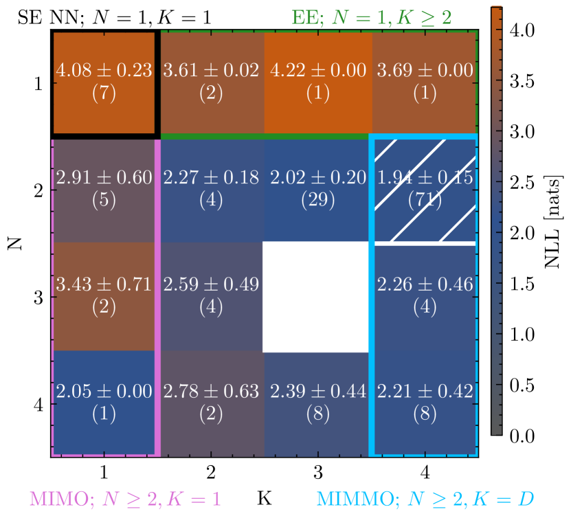
(a) NLL on TinyImageNet ID.

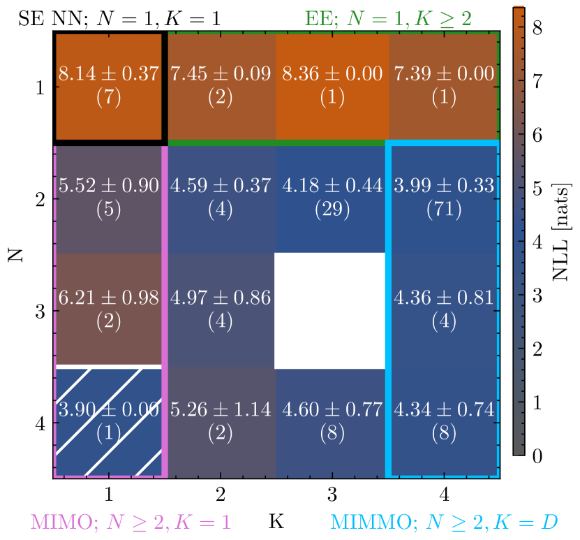
(b) NLL on TinyImageNet OOD.

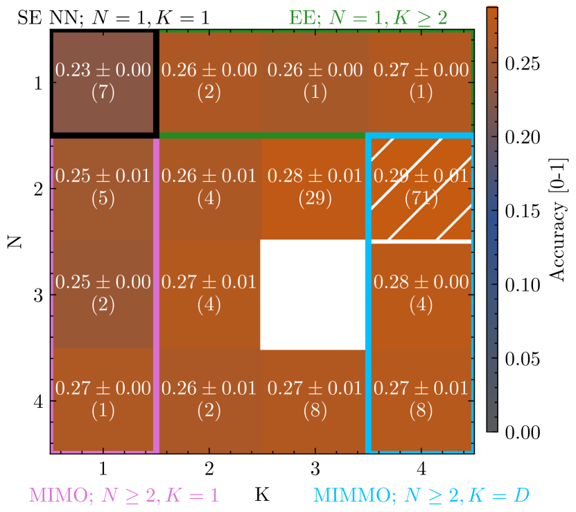
(c) Accuracy on TinyImageNet OOD.

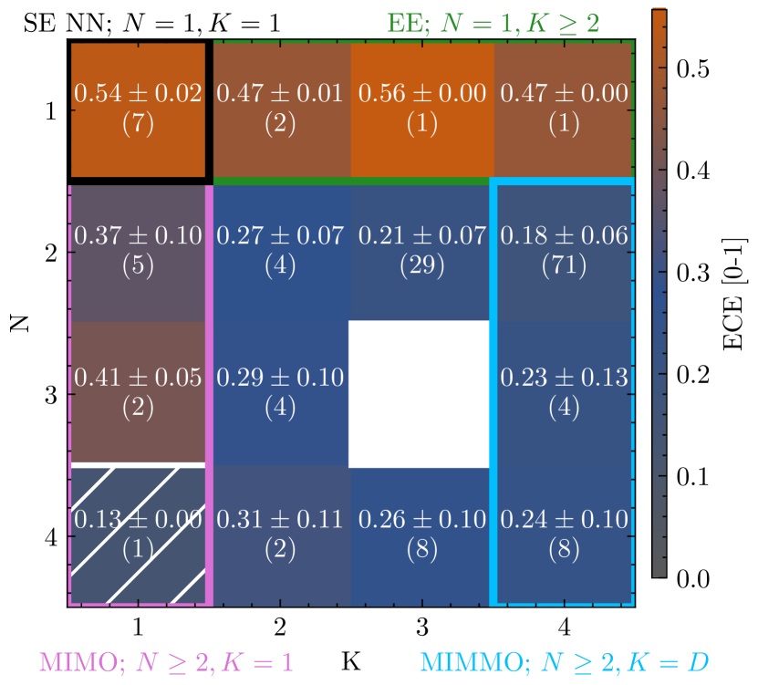
(d) ECE on TinyImageNet OOD.

Figure 9: Varying $N,K$ on TinyImageNet ID and OOD test sets. The upper number is the average performance over $N$, $K$ combinations. The number in brackets is the number of sampled configurations by HPO. White box means no configurations sampled for that $N$, $K$. Pattern signals best average performance. The coloured outlines signal the special cases for the generalised methods.

In Figures 9, 10, 11 and 12 we show the Varying $N,K$ on TinyImageNet, RetinaMNIST, PneumoniaMNIST and BloodMNIST datasets concerning different metrics. As discussed in the main part of the paper, there might be different suitable configurations for various metrics. We would point the reader’s attention to the OOD results across all datasets and the ID results where we have shown that the $N$ and $K$ are different.

10 SUPPLEMENTARY FOR DEPTH PREFERENCE

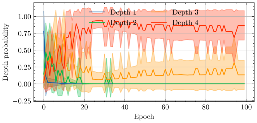
(a) $N=1$.

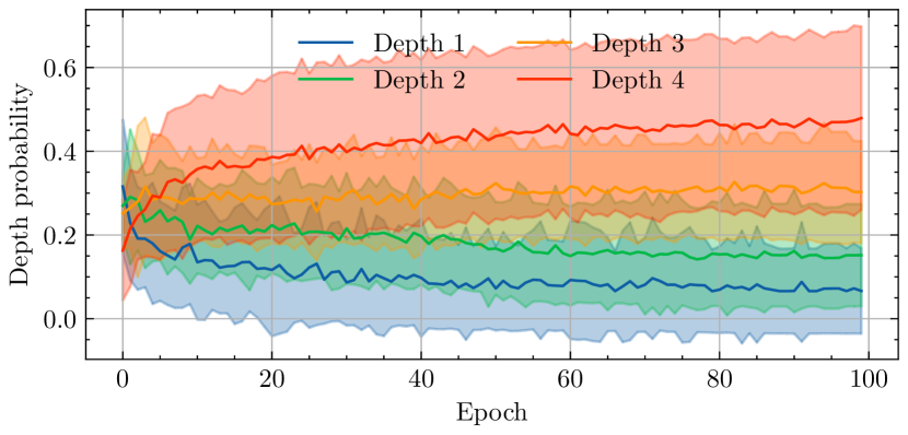
(b) $N=2$.

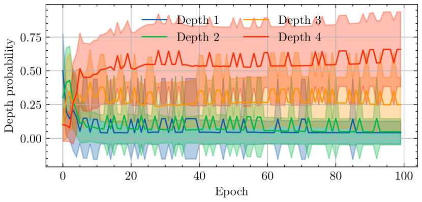
(c) $N=3$.

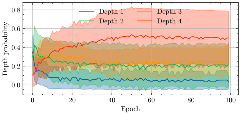
(d) $N=4$.

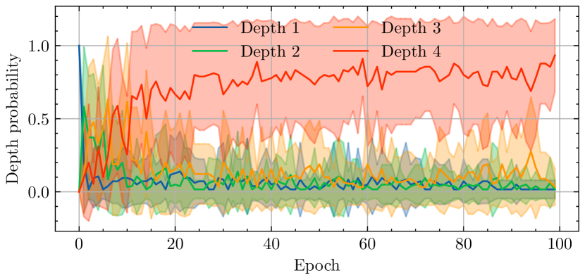
(e) $K=1$.

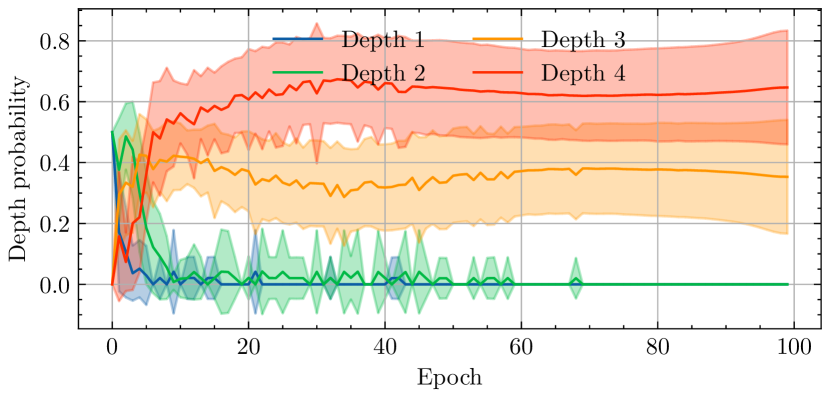
(f) $K=2$.

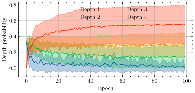
(g) $K=3$.

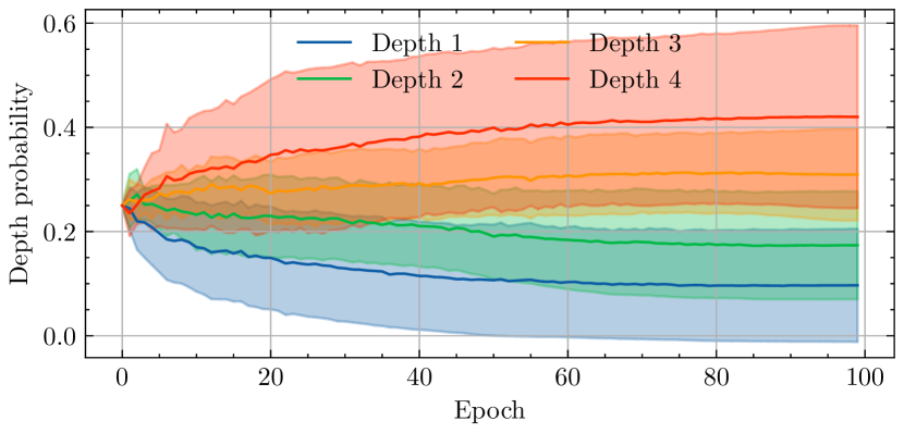
(h) $K=D$.

Figure 13: Depth preference during training when averaging over different $N$ and $K$ for TinyImageNet. The lines denote the mean trend, and the shaded regions denote the standard deviation across configurations.

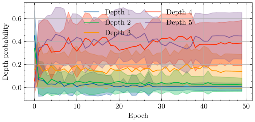
(a) $N=1$.

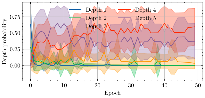
(b) $N=2$.

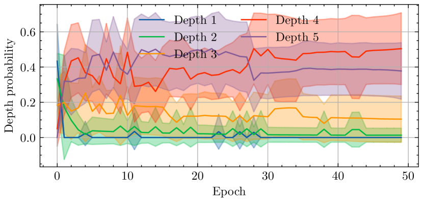
(c) $N=3$.

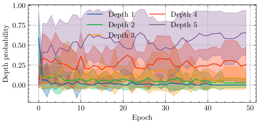
(d) $N=4$.

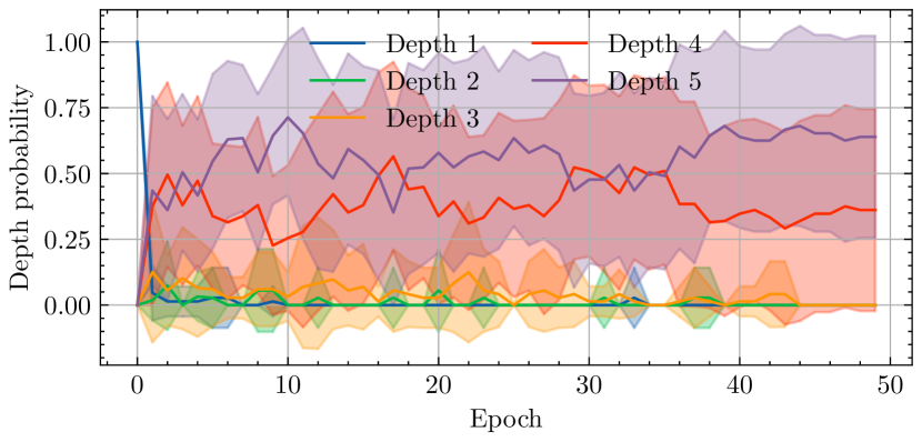
(e) $K=1$.

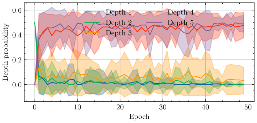
(f) $K=2$.

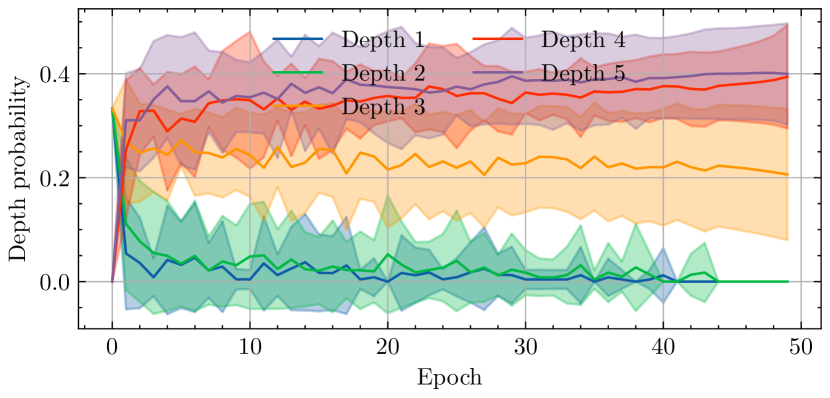
(g) $K=3$.

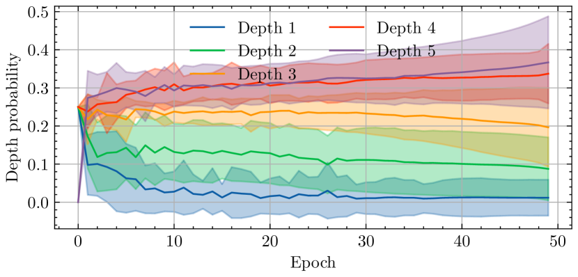
(h) $K=D$.

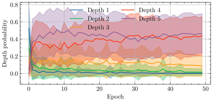
(i) Average over all $N$ and $K$.

Figure 15: Depth preference during training when averaging over different $N$ and $K$ for BloodMNIST. The lines denote the mean trend, and the shaded regions denote the standard deviation across configurations.

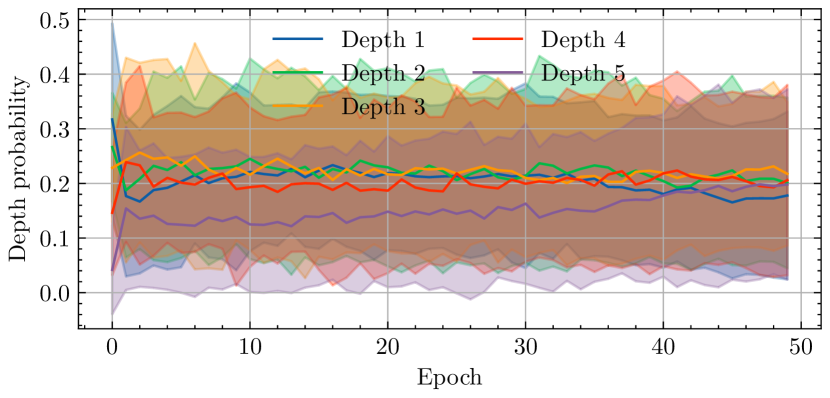
(a) $N=1$.

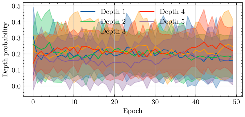
(b) $N=2$.

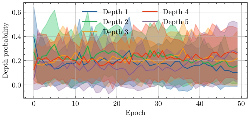
(c) $N=3$.

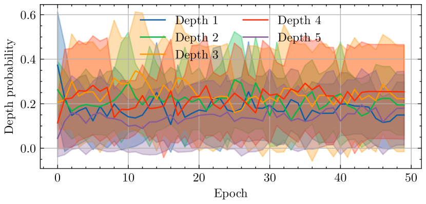
(d) $N=4$.

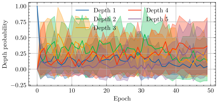
(e) $K=1$.

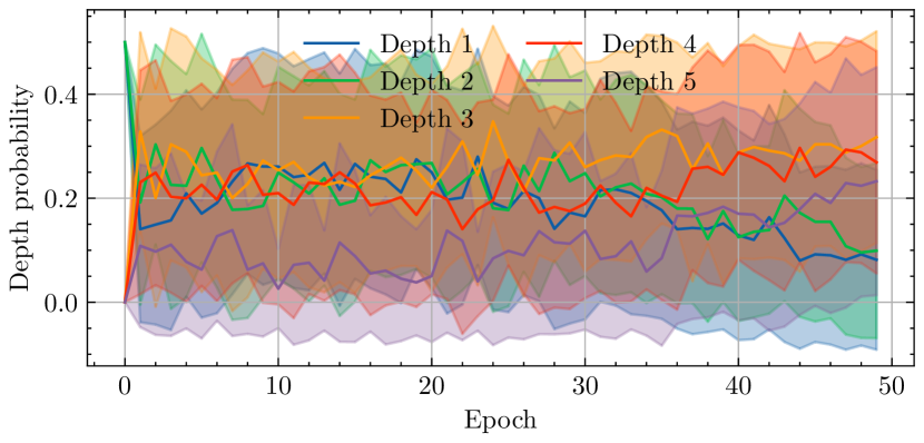
(f) $K=2$.

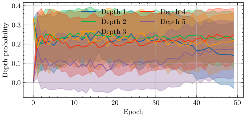
(g) $K=3$.

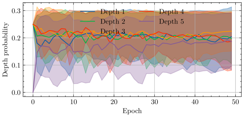
(h) $K=4$.

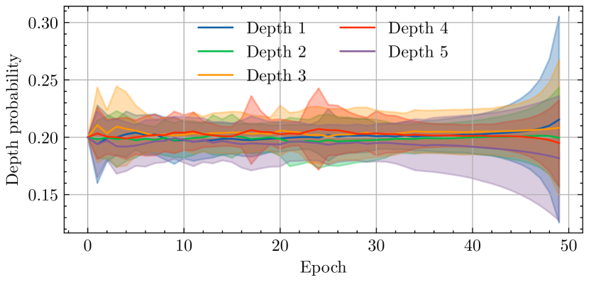
(i) $K=D$.

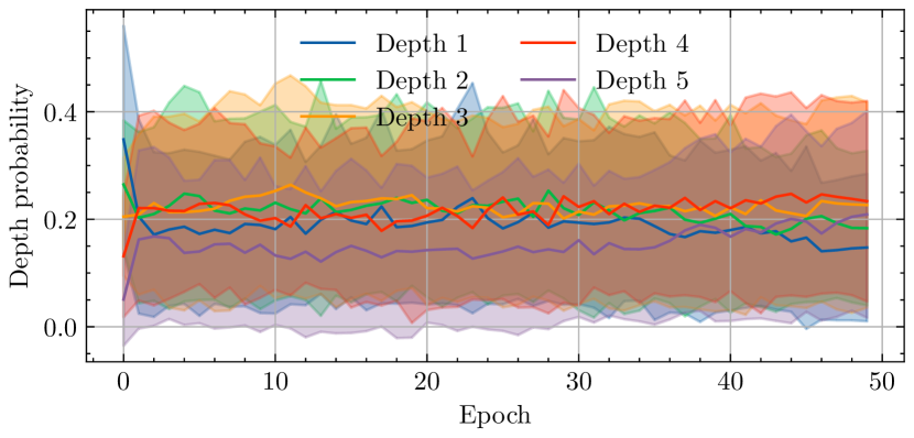
(j) Average over all $N$ and $K$.

Figure 16: Depth preference during training when averaging over different $N$ and $K$ for PneumoniaMNIST. The lines denote the mean trend, and the shaded regions denote the standard deviation across configurations.

In Figures 13, 14, 15 and 16, we show the depth preference for different $N$ and $K$ on TinyImageNet, RetinaMNIST, BloodMNIST and PneumoniaMNIST, respectively. We categorise the results according to $N$ and $K$ and show the average depth preference across all $K$ or $N$, respectively. The results show that the depth preference is consistent across different $N$ and $K$. However, there is a difference between backbone architectures. For example, RetinaMNIST and PneumoniaMNIST used ViT and FC backbones, respectively, and there was no clear preference for the depth, as seen in Figures 16 and 14. However, for BloodMNIST and TinyImageNet, which have convolutional backbones, the depth preference was evident towards the deeper layers, as seen in Figures 15 and 13.

11 SUPPLEMENTARY FOR HYPERPARAMETER SCHEDULES

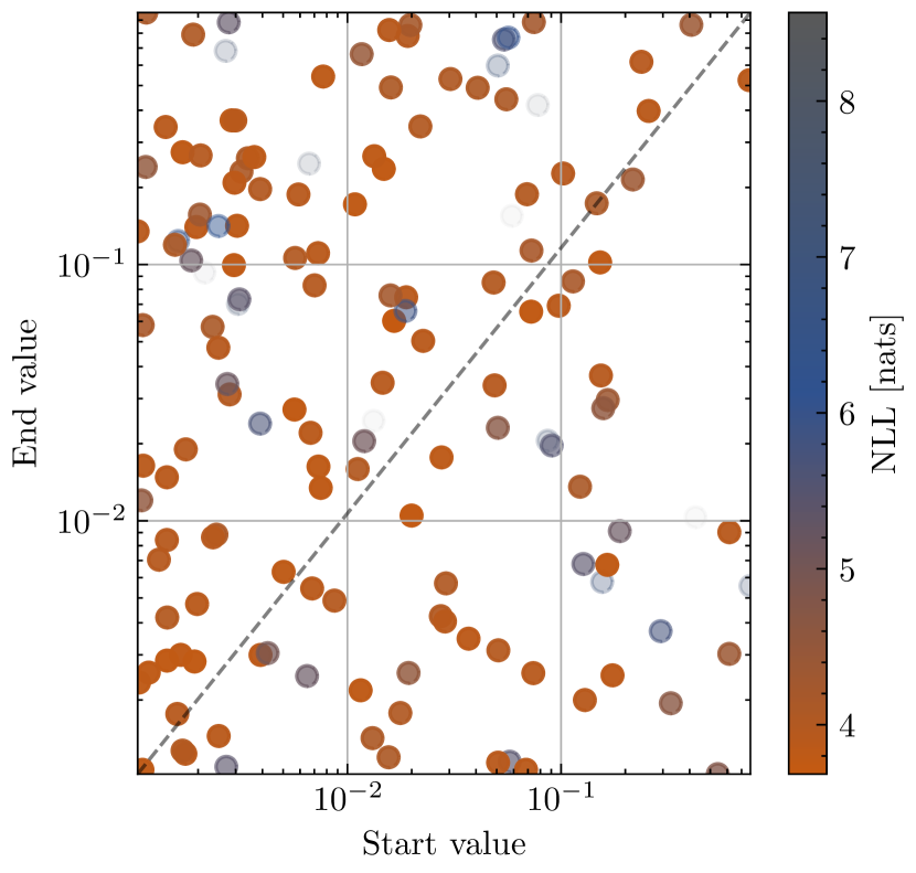
(a) Temperature for TinyImageNet OOD.

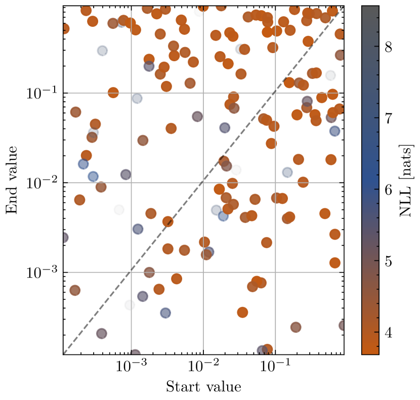
(b) Alpha for TinyImageNet OOD.

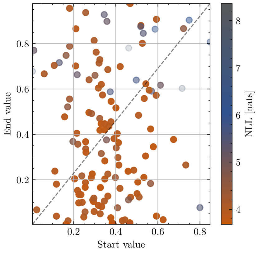
(c) Input repetition probability for TinyImageNet OOD.

Figure 17: HP tuning for TinyImageNet NLL on ID and OOD test sets.

Lastly, in Figures 17, 18, 19, 20 we show the HPs schedules for TinyImageNet, RetinaMNIST, BloodMNIST and PneumoniaMNIST datasets. As the Figures show, it is impossible to identify a clear trend for the HP start and end values, which are essentially dataset- and architecture-dependent. However, what is clear is that the HP schedules are essential since the HPO did not prefer points on a diagonal, which would indicate that the start and end values should stay the same.

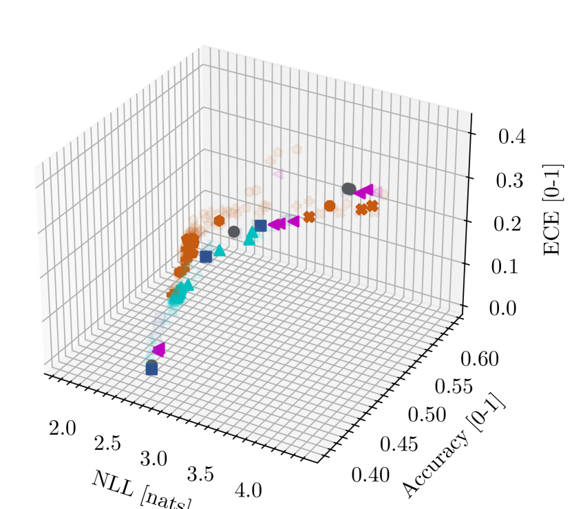
(a) TinyImageNet ID.

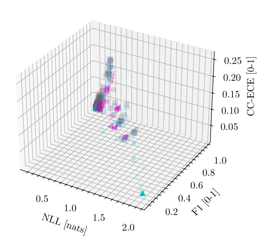
(b) BloodMNIST ID.

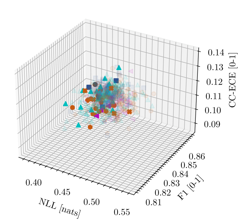
(c) PneumoniaMNIST ID.

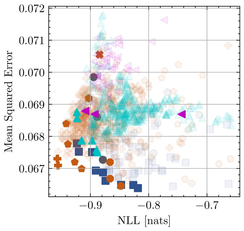
(d) RetinaMNIST ID.

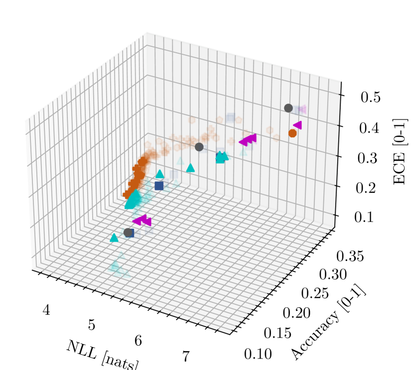
(e) TinyImageNet OOD.

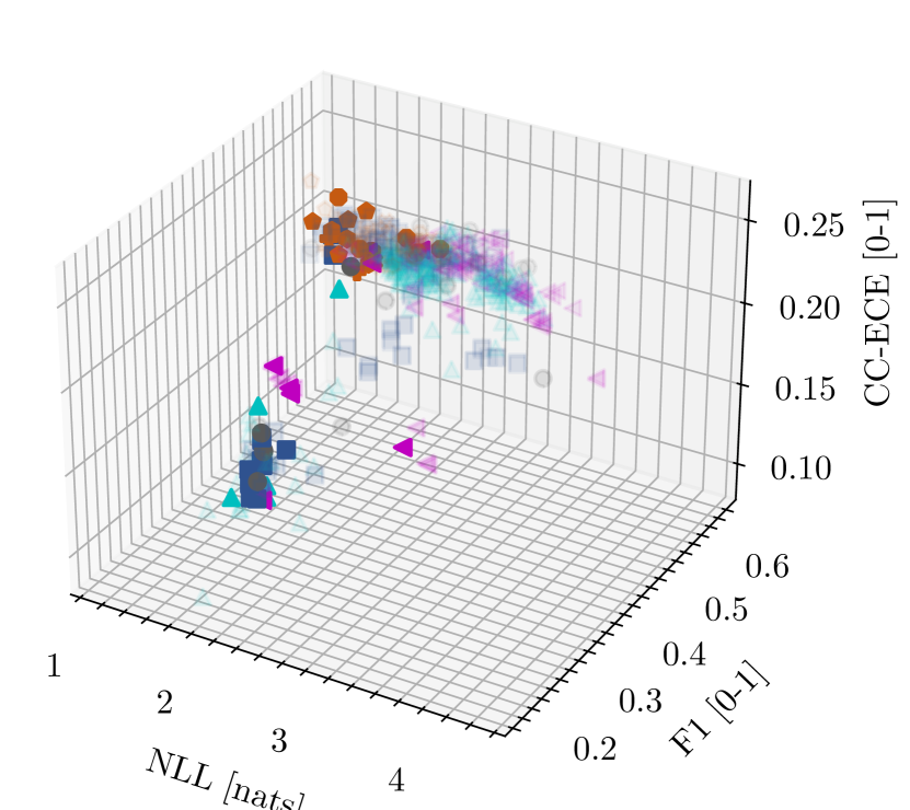
(f) BloodMNIST OOD.

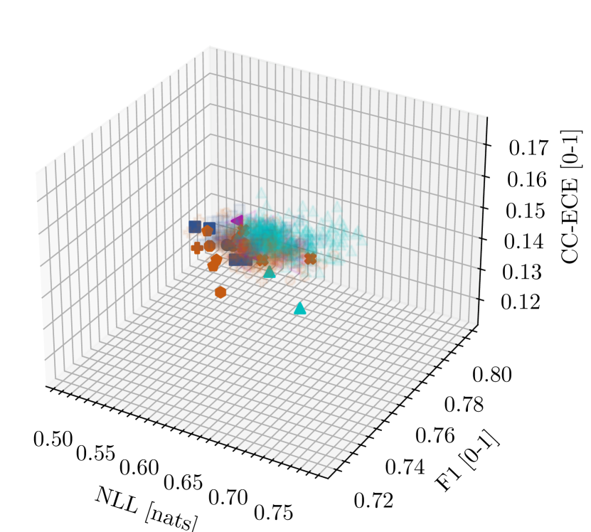
(g) PneumoniaMNIST OOD.

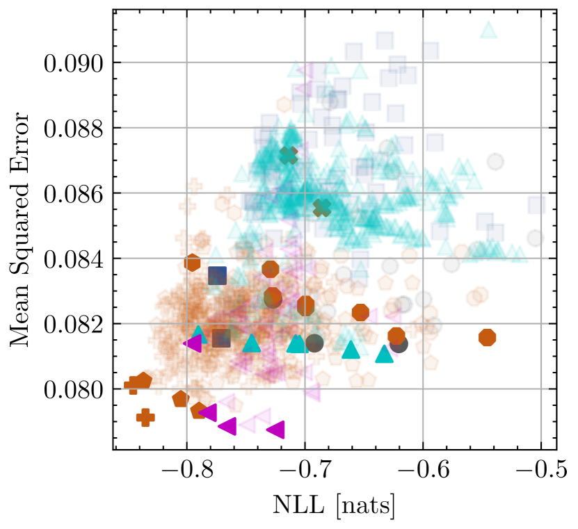
(h) RetinaMNIST OOD.

Figure 7: Comparison on TinyImageNet, BloodMNIST, PneumoniaMNIST, and RetinaMNIST across ID (upper row) and OOD (lower row) datasets, with respect to Standard NN $\newmoon$, NN Ensemble $\blacksquare$, SAE: I/B: $N\geq 2,2\leq K<D$ , EE: $N=1,K\geq 2$ , MIMMO: $N\geq 2,K=D$ , MIMO: $N\geq 2,K=1$ , SE NN: $N=1,K=1$ , MCD $\blacktriangle$, BE $\blacktriangleleft$. The plots contain all the configurations tried by hyperparameter optimisation. The high opacity configurations indicate the configurations used for the final evaluation over repeated seeds.

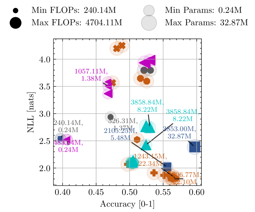
(a) TinyImageNet ID.

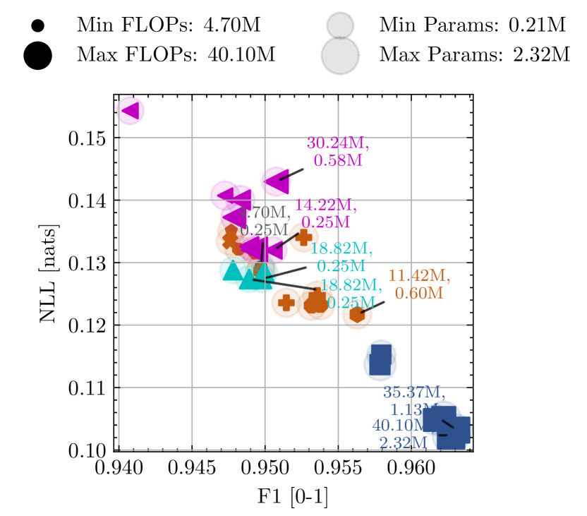
(b) BloodMNIST ID.

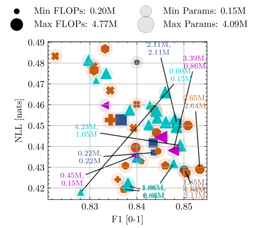
(c) PneumoniaMNIST ID.

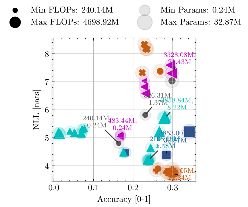
(d) TinyImageNet OOD.

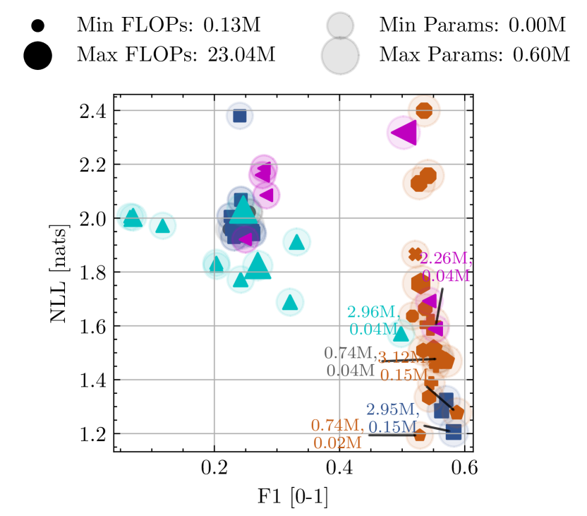
(e) BloodMNIST OOD.

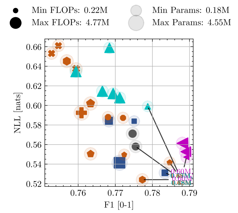
(f) PneumoniaMNIST OOD.

Figure 8: Comparison on TinyImageNet, BloodMNIST and PneumoniaMNIST across ID (upper row) and OOD (lower row) datasets, with respect to Standard NN $\newmoon$, NN Ensemble $\blacksquare$, SAE: I/B: $N\geq 2,2\leq K<D$ , EE: $N=1,K\geq 2$ , MIMMO: $N\geq 2,K=D$ , MIMO: $N\geq 2,K=1$ , SE NN: $N=1,K=1$ , MCD $\blacktriangle$, BE $\blacktriangleleft$. The size of the marker denotes the number of FLOPs, and the shaded region denotes the number of parameters. The first row of the caption denotes the number of FLOPs, and the second row denotes the number of parameters.

Table 1: Best results for empirically Pareto optimal configurations on TinyImageNet ID dataset. Each row represents the best configuration for each method for the first metric, the second metric, etc. The count represents how many configurations were in the Pareto front. The italic and underlined values represent the compared configurations in the main text, respectively. The bold values represent the best value across all methods for each metric.

Method Count NLL [nats] Accuracy [0-1] ECE [0-1] FLOPs [M] Params [M] Standard NN $\newmoon$ 4 2.540 $\pm$ 0.006 0.396 $\pm$ 0.001 0.010 $\pm$ 0.002 240.137 $\pm$ 0.000 0.241 $\pm$ 0.000 3.796 $\pm$ 0.025 0.531 $\pm$ 0.001 0.330 $\pm$ 0.002 963.251 $\pm$ 0.000 8.218 $\pm$ 0.000 2.540 $\pm$ 0.006 0.396 $\pm$ 0.001 0.010 $\pm$ 0.002 240.137 $\pm$ 0.000 0.241 $\pm$ 0.000 NN Ensemble $\blacksquare$ 3 2.022 $\pm$ 0.008 0.556 $\pm$ 0.001 0.037 $\pm$ 0.002 2105.251 $\pm$ 0.000 5.481 $\pm$ 0.000 2.388 $\pm$ 0.006 0.597 $\pm$ 0.002 0.083 $\pm$ 0.003 3853.002 $\pm$ 0.000 32.873 $\pm$ 0.000 2.538 $\pm$ 0.015 0.397 $\pm$ 0.003 0.009 $\pm$ 0.002 240.137 $\pm$ 0.000 0.241 $\pm$ 0.000 MCD $\blacktriangle$ 19 2.086 $\pm$ 0.009 0.505 $\pm$ 0.003 0.015 $\pm$ 0.003 2110.102 $\pm$ 0.000 1.370 $\pm$ 0.000 2.744 $\pm$ 0.020 0.530 $\pm$ 0.002 0.172 $\pm$ 0.004 3858.836 $\pm$ 0.000 8.218 $\pm$ 0.000 5.139 $\pm$ 0.002 0.012 $\pm$ 0.001 0.003 $\pm$ 0.001 3858.836 $\pm$ 0.000 8.218 $\pm$ 0.000 BE $\blacktriangleleft$ 7 2.520 $\pm$ 0.005 0.407 $\pm$ 0.003 0.032 $\pm$ 0.005 483.445 $\pm$ 0.000 0.244 $\pm$ 0.000 3.980 $\pm$ 0.020 0.530 $\pm$ 0.004 0.338 $\pm$ 0.002 3863.801 $\pm$ 0.000 8.259 $\pm$ 0.000 2.523 $\pm$ 0.011 0.406 $\pm$ 0.002 0.027 $\pm$ 0.003 966.889 $\pm$ 0.000 0.247 $\pm$ 0.000 MIMO; $N\geq 2,K=1$ 2 2.071 $\pm$ 0.048 0.505 $\pm$ 0.009 0.051 $\pm$ 0.014 1081.378 $\pm$ 81.796 12.078 $\pm$ 5.669 2.522 $\pm$ 0.048 0.511 $\pm$ 0.004 0.210 $\pm$ 0.003 1180.377 $\pm$ 0.000 21.488 $\pm$ 0.000 2.071 $\pm$ 0.048 0.505 $\pm$ 0.009 0.051 $\pm$ 0.014 1081.378 $\pm$ 81.796 12.078 $\pm$ 5.669 MIMMO; $N\geq 2,K=D$ 4 1.807 $\pm$ 0.013 0.563 $\pm$ 0.005 0.063 $\pm$ 0.003 1243.154 $\pm$ 0.000 22.338 $\pm$ 0.000 1.808 $\pm$ 0.003 0.569 $\pm$ 0.001 0.046 $\pm$ 0.002 1243.154 $\pm$ 0.000 22.338 $\pm$ 0.000 1.815 $\pm$ 0.016 0.561 $\pm$ 0.004 0.026 $\pm$ 0.003 1243.051 $\pm$ 0.000 22.235 $\pm$ 0.000 SE NN; $N=1,K=1$ 3 3.566 $\pm$ 0.056 0.474 $\pm$ 0.004 0.319 $\pm$ 0.006 1173.197 $\pm$ 0.000 21.384 $\pm$ 0.000 4.252 $\pm$ 0.011 0.488 $\pm$ 0.002 0.363 $\pm$ 0.002 1173.197 $\pm$ 0.000 21.384 $\pm$ 0.000 3.566 $\pm$ 0.056 0.474 $\pm$ 0.004 0.319 $\pm$ 0.006 1173.197 $\pm$ 0.000 21.384 $\pm$ 0.000 EE; $N=1,K\geq 2$ 2 3.596 $\pm$ 0.020 0.526 $\pm$ 0.005 0.337 $\pm$ 0.092 1181.852 $\pm$ 0.000 21.619 $\pm$ 0.000 3.596 $\pm$ 0.020 0.526 $\pm$ 0.005 0.337 $\pm$ 0.092 1181.852 $\pm$ 0.000 21.619 $\pm$ 0.000 3.596 $\pm$ 0.020 0.526 $\pm$ 0.005 0.337 $\pm$ 0.092 1181.852 $\pm$ 0.000 21.619 $\pm$ 0.000 I/B; $N\geq 2,2\leq K\leq D$ 5 1.801 $\pm$ 0.026 0.564 $\pm$ 0.009 0.040 $\pm$ 0.006 1206.773 $\pm$ 0.000 22.098 $\pm$ 0.000 1.801 $\pm$ 0.026 0.564 $\pm$ 0.009 0.040 $\pm$ 0.006 1206.773 $\pm$ 0.000 22.098 $\pm$ 0.000 2.068 $\pm$ 0.010 0.497 $\pm$ 0.003 0.018 $\pm$ 0.001 1196.418 $\pm$ 0.000 22.033 $\pm$ 0.000

Table 2: Best results for empirically Pareto optimal configurations on TinyImageNet OOD dataset. Each row represents the best configuration for each method for the first metric, the second metric, etc. The count represents how many configurations were in the Pareto front. The italic and underlined values represent the compared configurations in the main text, respectively. The bold values represent the best value across all methods for each metric.

Method Count NLL [nats] Accuracy [0-1] ECE [0-1] FLOPs [M] Params [M] Standard NN $\newmoon$ 3 4.803 $\pm$ 1.586 0.164 $\pm$ 0.104 0.157 $\pm$ 0.094 240.137 $\pm$ 0.000 0.241 $\pm$ 0.000 7.033 $\pm$ 2.485 0.298 $\pm$ 0.135 0.497 $\pm$ 0.105 1173.197 $\pm$ 0.000 21.384 $\pm$ 0.000 4.803 $\pm$ 1.586 0.164 $\pm$ 0.104 0.157 $\pm$ 0.094 240.137 $\pm$ 0.000 0.241 $\pm$ 0.000 NN Ensemble $\blacksquare$ 3 4.387 $\pm$ 1.809 0.284 $\pm$ 0.151 0.143 $\pm$ 0.090 2105.251 $\pm$ 0.000 5.481 $\pm$ 0.000 5.219 $\pm$ 2.330 0.342 $\pm$ 0.158 0.211 $\pm$ 0.100 3853.002 $\pm$ 0.000 32.873 $\pm$ 0.000 4.477 $\pm$ 1.460 0.182 $\pm$ 0.115 0.102 $\pm$ 0.070 960.548 $\pm$ 0.000 0.964 $\pm$ 0.000 MCD $\blacktriangle$ 26 4.180 $\pm$ 1.517 0.240 $\pm$ 0.136 0.134 $\pm$ 0.097 2110.102 $\pm$ 0.000 1.370 $\pm$ 0.000 5.731 $\pm$ 2.304 0.282 $\pm$ 0.143 0.317 $\pm$ 0.099 3858.836 $\pm$ 0.000 8.218 $\pm$ 0.000 5.158 $\pm$ 0.019 0.012 $\pm$ 0.001 0.002 $\pm$ 0.001 3858.836 $\pm$ 0.000 8.218 $\pm$ 0.000 BE $\blacktriangleleft$ 8 5.050 $\pm$ 1.891 0.168 $\pm$ 0.107 0.189 $\pm$ 0.112 966.889 $\pm$ 0.000 0.247 $\pm$ 0.000 7.302 $\pm$ 2.542 0.298 $\pm$ 0.136 0.446 $\pm$ 0.069 3528.084 $\pm$ 0.000 21.435 $\pm$ 0.000 5.050 $\pm$ 1.891 0.168 $\pm$ 0.107 0.189 $\pm$ 0.112 966.889 $\pm$ 0.000 0.247 $\pm$ 0.000 MIMO; $N\geq 2,K=1$ 1 3.902 $\pm$ 1.371 0.263 $\pm$ 0.136 0.122 $\pm$ 0.078 1081.378 $\pm$ 81.796 12.078 $\pm$ 5.669 3.902 $\pm$ 1.371 0.263 $\pm$ 0.136 0.122 $\pm$ 0.078 1081.378 $\pm$ 81.796 12.078 $\pm$ 5.669 3.902 $\pm$ 1.371 0.263 $\pm$ 0.136 0.122 $\pm$ 0.078 1081.378 $\pm$ 81.796 12.078 $\pm$ 5.669 MIMMO; $N\geq 2,K=D$ 5 3.686 $\pm$ 1.425 0.301 $\pm$ 0.151 0.138 $\pm$ 0.087 1243.051 $\pm$ 0.000 22.235 $\pm$ 0.000 3.704 $\pm$ 1.445 0.306 $\pm$ 0.153 0.129 $\pm$ 0.086 1243.154 $\pm$ 0.000 22.338 $\pm$ 0.000 3.697 $\pm$ 1.420 0.296 $\pm$ 0.152 0.106 $\pm$ 0.078 1243.154 $\pm$ 0.000 22.338 $\pm$ 0.000 SE NN; $N=1,K=1$ 4 7.324 $\pm$ 2.499 0.223 $\pm$ 0.127 0.494 $\pm$ 0.091 1173.197 $\pm$ 0.000 21.384 $\pm$ 0.000 8.162 $\pm$ 2.635 0.235 $\pm$ 0.129 0.546 $\pm$ 0.098 1173.197 $\pm$ 0.000 21.384 $\pm$ 0.000 7.324 $\pm$ 2.499 0.223 $\pm$ 0.127 0.494 $\pm$ 0.091 1173.197 $\pm$ 0.000 21.384 $\pm$ 0.000 EE; $N=1,K\geq 2$ 1 7.375 $\pm$ 2.668 0.268 $\pm$ 0.143 0.462 $\pm$ 0.089 1181.852 $\pm$ 0.000 21.619 $\pm$ 0.000 7.375 $\pm$ 2.668 0.268 $\pm$ 0.143 0.462 $\pm$ 0.089 1181.852 $\pm$ 0.000 21.619 $\pm$ 0.000 7.375 $\pm$ 2.668 0.268 $\pm$ 0.143 0.462 $\pm$ 0.089 1181.852 $\pm$ 0.000 21.619 $\pm$ 0.000 I/B; $N\geq 2,2\leq K\leq D$ 5 3.723 $\pm$ 1.443 0.303 $\pm$ 0.151 0.164 $\pm$ 0.088 1206.773 $\pm$ 0.000 22.098 $\pm$ 0.000 3.723 $\pm$ 1.443 0.303 $\pm$ 0.151 0.164 $\pm$ 0.088 1206.773 $\pm$ 0.000 22.098 $\pm$ 0.000 3.849 $\pm$ 1.334 0.259 $\pm$ 0.133 0.120 $\pm$ 0.092 1221.467 $\pm$ 0.044 22.640 $\pm$ 0.044

Table 3: Best results for empirically Pareto optimal configurations on BloodMNIST ID dataset. Each row represents the best configuration for each method for the first metric, the second metric, etc. The count represents how many configurations were in the Pareto front. The italic and underlined values represent the compared configurations in the main text, respectively. The bold values represent the best value across all methods for each metric.

Method Count NLL [nats] F1 [0-1] CC-ECE [0-1] FLOPs [M] Params [M] Standard NN $\newmoon$ 1 0.129 $\pm$ 0.004 0.950 $\pm$ 0.003 0.023 $\pm$ 0.003 4.697 $\pm$ 0.000 0.246 $\pm$ 0.000 0.129 $\pm$ 0.004 0.950 $\pm$ 0.003 0.023 $\pm$ 0.003 4.697 $\pm$ 0.000 0.246 $\pm$ 0.000 0.129 $\pm$ 0.004 0.950 $\pm$ 0.003 0.023 $\pm$ 0.003 4.697 $\pm$ 0.000 0.246 $\pm$ 0.000 NN Ensemble $\blacksquare$ 6 0.102 $\pm$ 0.002 0.963 $\pm$ 0.001 0.023 $\pm$ 0.002 40.102 $\pm$ 0.000 2.315 $\pm$ 0.000 0.103 $\pm$ 0.003 0.963 $\pm$ 0.001 0.023 $\pm$ 0.002 35.371 $\pm$ 0.000 1.134 $\pm$ 0.000 0.115 $\pm$ 0.003 0.958 $\pm$ 0.001 0.020 $\pm$ 0.001 17.686 $\pm$ 0.000 0.567 $\pm$ 0.000 MCD $\blacktriangle$ 5 0.127 $\pm$ 0.002 0.949 $\pm$ 0.001 0.023 $\pm$ 0.001 18.820 $\pm$ 0.000 0.246 $\pm$ 0.000 0.129 $\pm$ 0.002 0.950 $\pm$ 0.003 0.020 $\pm$ 0.001 18.820 $\pm$ 0.000 0.246 $\pm$ 0.000 0.129 $\pm$ 0.002 0.950 $\pm$ 0.003 0.020 $\pm$ 0.001 18.820 $\pm$ 0.000 0.246 $\pm$ 0.000 BE $\blacktriangleleft$ 8 0.132 $\pm$ 0.002 0.951 $\pm$ 0.004 0.022 $\pm$ 0.002 14.218 $\pm$ 0.000 0.249 $\pm$ 0.000 0.143 $\pm$ 0.004 0.951 $\pm$ 0.004 0.028 $\pm$ 0.001 30.243 $\pm$ 0.000 0.583 $\pm$ 0.000 0.132 $\pm$ 0.002 0.951 $\pm$ 0.004 0.022 $\pm$ 0.002 14.218 $\pm$ 0.000 0.249 $\pm$ 0.000 MIMO; $N\geq 2,K=1$ 2 0.122 $\pm$ 0.005 0.956 $\pm$ 0.004 0.022 $\pm$ 0.001 11.424 $\pm$ 0.000 0.600 $\pm$ 0.000 0.122 $\pm$ 0.005 0.956 $\pm$ 0.004 0.022 $\pm$ 0.001 11.424 $\pm$ 0.000 0.600 $\pm$ 0.000 0.122 $\pm$ 0.005 0.956 $\pm$ 0.004 0.022 $\pm$ 0.001 11.424 $\pm$ 0.000 0.600 $\pm$ 0.000 MIMMO; $N\geq 2,K=D$ 1 0.135 $\pm$ 0.006 0.948 $\pm$ 0.003 0.029 $\pm$ 0.001 5.621 $\pm$ 0.289 0.212 $\pm$ 0.072 0.135 $\pm$ 0.006 0.948 $\pm$ 0.003 0.029 $\pm$ 0.001 5.621 $\pm$ 0.289 0.212 $\pm$ 0.072 0.135 $\pm$ 0.006 0.948 $\pm$ 0.003 0.029 $\pm$ 0.001 5.621 $\pm$ 0.289 0.212 $\pm$ 0.072 SE NN; $N=1,K=1$ 1 0.133 $\pm$ 0.006 0.948 $\pm$ 0.004 0.022 $\pm$ 0.001 9.468 $\pm$ 0.558 0.440 $\pm$ 0.139 0.133 $\pm$ 0.006 0.948 $\pm$ 0.004 0.022 $\pm$ 0.001 9.468 $\pm$ 0.558 0.440 $\pm$ 0.139 0.133 $\pm$ 0.006 0.948 $\pm$ 0.004 0.022 $\pm$ 0.001 9.468 $\pm$ 0.558 0.440 $\pm$ 0.139 EE; $N=1,K\geq 2$ 4 0.123 $\pm$ 0.006 0.953 $\pm$ 0.004 0.025 $\pm$ 0.004 10.465 $\pm$ 0.132 0.610 $\pm$ 0.002 0.123 $\pm$ 0.005 0.954 $\pm$ 0.004 0.024 $\pm$ 0.002 10.237 $\pm$ 0.000 0.606 $\pm$ 0.000 0.132 $\pm$ 0.002 0.948 $\pm$ 0.001 0.021 $\pm$ 0.001 5.789 $\pm$ 0.000 0.336 $\pm$ 0.000 I/B; $N\geq 2,2\leq K\leq D$ 3 0.124 $\pm$ 0.003 0.951 $\pm$ 0.002 0.024 $\pm$ 0.002 10.539 $\pm$ 0.000 0.599 $\pm$ 0.000 0.125 $\pm$ 0.006 0.954 $\pm$ 0.003 0.026 $\pm$ 0.003 11.499 $\pm$ 0.071 0.608 $\pm$ 0.004 0.124 $\pm$ 0.003 0.951 $\pm$ 0.002 0.024 $\pm$ 0.002 10.539 $\pm$ 0.000 0.599 $\pm$ 0.000

Table 4: Best results for empirically Pareto optimal configurations on BloodMNIST OOD dataset. Each row represents the best configuration for each method for the first metric, the second metric, etc. The count represents how many configurations were in the Pareto front. The italic and underlined values represent the compared configurations in the main text, respectively. The bold values represent the best value across all methods for each metric.

Method Count NLL [nats] F1 [0-1] CC-ECE [0-1] FLOPs [M] Params [M] Standard NN $\newmoon$ 5 1.478 $\pm$ 1.255 0.560 $\pm$ 0.258 0.187 $\pm$ 0.092 0.737 $\pm$ 0.000 0.037 $\pm$ 0.000 1.478 $\pm$ 1.255 0.560 $\pm$ 0.258 0.187 $\pm$ 0.092 0.737 $\pm$ 0.000 0.037 $\pm$ 0.000 1.959 $\pm$ 0.990 0.223 $\pm$ 0.080 0.140 $\pm$ 0.025 0.128 $\pm$ 0.000 0.000 $\pm$ 0.000 NN Ensemble $\blacksquare$ 17 1.206 $\pm$ 1.040 0.582 $\pm$ 0.269 0.198 $\pm$ 0.078 2.948 $\pm$ 0.000 0.147 $\pm$ 0.000 1.206 $\pm$ 1.040 0.582 $\pm$ 0.269 0.198 $\pm$ 0.078 2.948 $\pm$ 0.000 0.147 $\pm$ 0.000 2.006 $\pm$ 1.530 0.225 $\pm$ 0.109 0.129 $\pm$ 0.030 0.256 $\pm$ 0.000 0.000 $\pm$ 0.000 MCD $\blacktriangle$ 11 1.571 $\pm$ 1.203 0.498 $\pm$ 0.221 0.182 $\pm$ 0.065 2.962 $\pm$ 0.000 0.037 $\pm$ 0.000 1.571 $\pm$ 1.203 0.498 $\pm$ 0.221 0.182 $\pm$ 0.065 2.962 $\pm$ 0.000 0.037 $\pm$ 0.000 2.005 $\pm$ 0.001 0.065 $\pm$ 0.004 0.011 $\pm$ 0.005 0.842 $\pm$ 0.000 0.000 $\pm$ 0.000 BE $\blacktriangleleft$ 13 1.589 $\pm$ 1.425 0.553 $\pm$ 0.262 0.188 $\pm$ 0.095 2.259 $\pm$ 0.000 0.038 $\pm$ 0.000 1.589 $\pm$ 1.425 0.553 $\pm$ 0.262 0.188 $\pm$ 0.095 2.259 $\pm$ 0.000 0.038 $\pm$ 0.000 1.921 $\pm$ 1.127 0.249 $\pm$ 0.077 0.142 $\pm$ 0.026 0.270 $\pm$ 0.000 0.000 $\pm$ 0.000 MIMO; $N\geq 2,K=1$ 4 1.335 $\pm$ 1.217 0.543 $\pm$ 0.265 0.201 $\pm$ 0.074 3.327 $\pm$ 0.009 0.150 $\pm$ 0.002 1.485 $\pm$ 1.445 0.556 $\pm$ 0.289 0.190 $\pm$ 0.091 6.767 $\pm$ 0.019 0.334 $\pm$ 0.005 1.485 $\pm$ 1.445 0.556 $\pm$ 0.289 0.190 $\pm$ 0.091 6.767 $\pm$ 0.019 0.334 $\pm$ 0.005 MIMMO; $N\geq 2,K=D$ 4 1.194 $\pm$ 0.849 0.528 $\pm$ 0.233 0.208 $\pm$ 0.044 0.741 $\pm$ 0.005 0.019 $\pm$ 0.000 1.277 $\pm$ 1.422 0.587 $\pm$ 0.281 0.179 $\pm$ 0.094 3.116 $\pm$ 0.000 0.153 $\pm$ 0.000 1.277 $\pm$ 1.422 0.587 $\pm$ 0.281 0.179 $\pm$ 0.094 3.116 $\pm$ 0.000 0.153 $\pm$ 0.000 SE NN; $N=1,K=1$ 1 1.866 $\pm$ 1.869 0.521 $\pm$ 0.267 0.201 $\pm$ 0.099 0.719 $\pm$ 0.030 0.032 $\pm$ 0.008 1.866 $\pm$ 1.869 0.521 $\pm$ 0.267 0.201 $\pm$ 0.099 0.719 $\pm$ 0.030 0.032 $\pm$ 0.008 1.866 $\pm$ 1.869 0.521 $\pm$ 0.267 0.201 $\pm$ 0.099 0.719 $\pm$ 0.030 0.032 $\pm$ 0.008 EE; $N=1,K\geq 2$ 5 1.636 $\pm$ 1.412 0.516 $\pm$ 0.272 0.229 $\pm$ 0.055 0.792 $\pm$ 0.020 0.040 $\pm$ 0.000 2.158 $\pm$ 2.128 0.541 $\pm$ 0.290 0.201 $\pm$ 0.095 5.213 $\pm$ 0.000 0.279 $\pm$ 0.000 1.664 $\pm$ 1.409 0.537 $\pm$ 0.283 0.197 $\pm$ 0.094 2.672 $\pm$ 0.000 0.150 $\pm$ 0.000 I/B; $N\geq 2,2\leq K\leq D$ 3 1.387 $\pm$ 1.373 0.547 $\pm$ 0.266 0.198 $\pm$ 0.069 1.083 $\pm$ 0.005 0.040 $\pm$ 0.000 1.451 $\pm$ 1.529 0.554 $\pm$ 0.265 0.185 $\pm$ 0.083 1.075 $\pm$ 0.000 0.040 $\pm$ 0.000 1.451 $\pm$ 1.529 0.554 $\pm$ 0.265 0.185 $\pm$ 0.083 1.075 $\pm$ 0.000 0.040 $\pm$ 0.000

Table 5: Best results for empirically Pareto optimal configurations on PneumoniaMNIST ID dataset. Each row represents the best configuration for each method for the first metric, the second metric, etc. The count represents how many configurations were in the Pareto front. The italic and underlined values represent the compared configurations in the main text, respectively. The bold values represent the best value across all methods for each metric.

Method Count NLL [nats] F1 [0-1] CC-ECE [0-1] FLOPs [M] Params [M] Standard NN $\newmoon$ 2 0.429 $\pm$ 0.015 0.850 $\pm$ 0.007 0.107 $\pm$ 0.006 1.850 $\pm$ 0.000 1.844 $\pm$ 0.000 0.429 $\pm$ 0.015 0.850 $\pm$ 0.007 0.107 $\pm$ 0.006 1.850 $\pm$ 0.000 1.844 $\pm$ 0.000 0.429 $\pm$ 0.015 0.850 $\pm$ 0.007 0.107 $\pm$ 0.006 1.850 $\pm$ 0.000 1.844 $\pm$ 0.000 NN Ensemble $\blacksquare$ 4 0.437 $\pm$ 0.018 0.844 $\pm$ 0.006 0.106 $\pm$ 0.002 0.217 $\pm$ 0.000 0.215 $\pm$ 0.000 0.451 $\pm$ 0.024 0.848 $\pm$ 0.011 0.112 $\pm$ 0.003 2.111 $\pm$ 0.000 2.106 $\pm$ 0.000 0.437 $\pm$ 0.018 0.844 $\pm$ 0.006 0.106 $\pm$ 0.002 0.217 $\pm$ 0.000 0.215 $\pm$ 0.000 MCD $\blacktriangle$ 20 0.418 $\pm$ 0.017 0.828 $\pm$ 0.003 0.112 $\pm$ 0.008 0.595 $\pm$ 0.000 0.148 $\pm$ 0.000 0.440 $\pm$ 0.030 0.849 $\pm$ 0.008 0.108 $\pm$ 0.004 4.229 $\pm$ 0.000 1.053 $\pm$ 0.000 0.678 $\pm$ 0.002 0.385 $\pm$ 0.000 0.042 $\pm$ 0.002 0.595 $\pm$ 0.000 0.148 $\pm$ 0.000 BE $\blacktriangleleft$ 4 0.436 $\pm$ 0.011 0.840 $\pm$ 0.010 0.109 $\pm$ 0.009 0.450 $\pm$ 0.000 0.153 $\pm$ 0.000 0.438 $\pm$ 0.018 0.848 $\pm$ 0.007 0.106 $\pm$ 0.010 3.388 $\pm$ 0.000 0.861 $\pm$ 0.000 0.444 $\pm$ 0.026 0.845 $\pm$ 0.014 0.103 $\pm$ 0.010 4.774 $\pm$ 0.000 1.604 $\pm$ 0.000 MIMO; $N\geq 2,K=1$ 3 0.431 $\pm$ 0.010 0.838 $\pm$ 0.005 0.105 $\pm$ 0.010 1.418 $\pm$ 0.033 1.416 $\pm$ 0.033 0.431 $\pm$ 0.010 0.838 $\pm$ 0.005 0.105 $\pm$ 0.010 1.418 $\pm$ 0.033 1.416 $\pm$ 0.033 0.431 $\pm$ 0.010 0.838 $\pm$ 0.005 0.105 $\pm$ 0.010 1.418 $\pm$ 0.033 1.416 $\pm$ 0.033 MIMMO; $N\geq 2,K=D$ 4 0.419 $\pm$ 0.025 0.837 $\pm$ 0.008 0.106 $\pm$ 0.009 1.660 $\pm$ 0.000 1.656 $\pm$ 0.000 0.431 $\pm$ 0.017 0.846 $\pm$ 0.005 0.104 $\pm$ 0.009 2.062 $\pm$ 0.075 2.057 $\pm$ 0.075 0.431 $\pm$ 0.017 0.846 $\pm$ 0.005 0.104 $\pm$ 0.009 2.062 $\pm$ 0.075 2.057 $\pm$ 0.075 SE NN; $N=1,K=1$ 5 0.449 $\pm$ 0.029 0.839 $\pm$ 0.016 0.109 $\pm$ 0.009 1.519 $\pm$ 0.220 1.515 $\pm$ 0.219 0.460 $\pm$ 0.049 0.840 $\pm$ 0.010 0.114 $\pm$ 0.011 1.029 $\pm$ 0.194 1.026 $\pm$ 0.193 0.449 $\pm$ 0.029 0.839 $\pm$ 0.016 0.109 $\pm$ 0.009 1.519 $\pm$ 0.220 1.515 $\pm$ 0.219 EE; $N=1,K\geq 2$ 7 0.427 $\pm$ 0.029 0.850 $\pm$ 0.013 0.097 $\pm$ 0.009 2.115 $\pm$ 0.000 2.109 $\pm$ 0.000 0.429 $\pm$ 0.028 0.853 $\pm$ 0.008 0.105 $\pm$ 0.008 2.645 $\pm$ 0.000 2.638 $\pm$ 0.000 0.427 $\pm$ 0.029 0.850 $\pm$ 0.013 0.097 $\pm$ 0.009 2.115 $\pm$ 0.000 2.109 $\pm$ 0.000 I/B; $N\geq 2,2\leq K\leq D$ 2 0.424 $\pm$ 0.036 0.836 $\pm$ 0.013 0.106 $\pm$ 0.019 0.549 $\pm$ 0.000 0.547 $\pm$ 0.000 0.424 $\pm$ 0.036 0.836 $\pm$ 0.013 0.106 $\pm$ 0.019 0.549 $\pm$ 0.000 0.547 $\pm$ 0.000 0.453 $\pm$ 0.058 0.834 $\pm$ 0.018 0.104 $\pm$ 0.017 4.094 $\pm$ 0.132 4.088 $\pm$ 0.132

Table 6: Best results for empirically Pareto optimal configurations on PneumoniaMNIST OOD dataset. Each row represents the best configuration for each method for the first metric, the second metric, etc. The count represents how many configurations were in the Pareto front. The italic and underlined values represent the compared configurations in the main text, respectively. The bold values represent the best value across all methods for each metric.

Method Count NLL [nats] F1 [0-1] CC-ECE [0-1] FLOPs [M] Params [M] Standard NN $\newmoon$ 2 0.558 $\pm$ 0.184 0.775 $\pm$ 0.100 0.133 $\pm$ 0.041 1.585 $\pm$ 0.000 1.581 $\pm$ 0.000 0.558 $\pm$ 0.184 0.775 $\pm$ 0.100 0.133 $\pm$ 0.041 1.585 $\pm$ 0.000 1.581 $\pm$ 0.000 0.558 $\pm$ 0.184 0.775 $\pm$ 0.100 0.133 $\pm$ 0.041 1.585 $\pm$ 0.000 1.581 $\pm$ 0.000 NN Ensemble $\blacksquare$ 4 0.531 $\pm$ 0.195 0.783 $\pm$ 0.096 0.135 $\pm$ 0.042 0.867 $\pm$ 0.000 0.861 $\pm$ 0.000 0.531 $\pm$ 0.195 0.783 $\pm$ 0.096 0.135 $\pm$ 0.042 0.867 $\pm$ 0.000 0.861 $\pm$ 0.000 0.584 $\pm$ 0.247 0.775 $\pm$ 0.100 0.133 $\pm$ 0.044 0.217 $\pm$ 0.000 0.215 $\pm$ 0.000 MCD $\blacktriangle$ 8 0.599 $\pm$ 0.415 0.779 $\pm$ 0.104 0.131 $\pm$ 0.062 0.733 $\pm$ 0.000 0.182 $\pm$ 0.000 0.599 $\pm$ 0.415 0.779 $\pm$ 0.104 0.131 $\pm$ 0.062 0.733 $\pm$ 0.000 0.182 $\pm$ 0.000 0.678 $\pm$ 0.005 0.385 $\pm$ 0.000 0.049 $\pm$ 0.021 0.595 $\pm$ 0.000 0.148 $\pm$ 0.000 BE $\blacktriangleleft$ 3 0.547 $\pm$ 0.171 0.789 $\pm$ 0.082 0.126 $\pm$ 0.042 0.601 $\pm$ 0.000 0.599 $\pm$ 0.000 0.547 $\pm$ 0.171 0.789 $\pm$ 0.082 0.126 $\pm$ 0.042 0.601 $\pm$ 0.000 0.599 $\pm$ 0.000 0.561 $\pm$ 0.210 0.788 $\pm$ 0.089 0.125 $\pm$ 0.045 4.774 $\pm$ 0.000 1.604 $\pm$ 0.000 MIMO; $N\geq 2,K=1$ 2 0.524 $\pm$ 0.223 0.777 $\pm$ 0.098 0.125 $\pm$ 0.050 1.418 $\pm$ 0.033 1.416 $\pm$ 0.033 0.524 $\pm$ 0.223 0.777 $\pm$ 0.098 0.125 $\pm$ 0.050 1.418 $\pm$ 0.033 1.416 $\pm$ 0.033 0.524 $\pm$ 0.223 0.777 $\pm$ 0.098 0.125 $\pm$ 0.050 1.418 $\pm$ 0.033 1.416 $\pm$ 0.033 MIMMO; $N\geq 2,K=D$ 4 0.542 $\pm$ 0.299 0.785 $\pm$ 0.108 0.128 $\pm$ 0.063 0.682 $\pm$ 0.000 0.680 $\pm$ 0.000 0.542 $\pm$ 0.299 0.785 $\pm$ 0.108 0.128 $\pm$ 0.063 0.682 $\pm$ 0.000 0.680 $\pm$ 0.000 0.542 $\pm$ 0.299 0.785 $\pm$ 0.108 0.128 $\pm$ 0.063 0.682 $\pm$ 0.000 0.680 $\pm$ 0.000 SE NN; $N=1,K=1$ 3 0.637 $\pm$ 0.280 0.759 $\pm$ 0.107 0.147 $\pm$ 0.051 1.519 $\pm$ 0.220 1.515 $\pm$ 0.219 0.637 $\pm$ 0.280 0.759 $\pm$ 0.107 0.147 $\pm$ 0.051 1.519 $\pm$ 0.220 1.515 $\pm$ 0.219 0.637 $\pm$ 0.280 0.759 $\pm$ 0.107 0.147 $\pm$ 0.051 1.519 $\pm$ 0.220 1.515 $\pm$ 0.219 EE; $N=1,K\geq 2$ 2 0.587 $\pm$ 0.238 0.772 $\pm$ 0.110 0.136 $\pm$ 0.053 0.715 $\pm$ 0.029 0.711 $\pm$ 0.029 0.587 $\pm$ 0.238 0.772 $\pm$ 0.110 0.136 $\pm$ 0.053 0.715 $\pm$ 0.029 0.711 $\pm$ 0.029 0.588 $\pm$ 0.257 0.768 $\pm$ 0.108 0.136 $\pm$ 0.045 0.798 $\pm$ 0.000 0.795 $\pm$ 0.000 I/B; $N\geq 2,2\leq K\leq D$ 1 0.592 $\pm$ 0.248 0.761 $\pm$ 0.110 0.138 $\pm$ 0.051 4.094 $\pm$ 0.132 4.088 $\pm$ 0.132 0.592 $\pm$ 0.248 0.761 $\pm$ 0.110 0.138 $\pm$ 0.051 4.094 $\pm$ 0.132 4.088 $\pm$ 0.132 0.592 $\pm$ 0.248 0.761 $\pm$ 0.110 0.138 $\pm$ 0.051 4.094 $\pm$ 0.132 4.088 $\pm$ 0.132

Table 7: Best results for empirically Pareto optimal configurations on RetinaMNIST ID dataset. Each row represents the best configuration for each method for the first metric, the second metric, etc. The count represents how many configurations were in the Pareto front. The italic and underlined values represent the compared configurations in the main text, respectively. The bold values represent the best value across all methods for each metric.

Method Count NLL [nats] MSE FLOPs [M] Params [M] Standard NN $\newmoon$ 3 -0.891 $\pm$ 0.008 0.069 $\pm$ 0.001 15.315 $\pm$ 0.000 0.246 $\pm$ 0.000 -0.843 $\pm$ 0.032 0.068 $\pm$ 0.001 58.925 $\pm$ 0.000 0.912 $\pm$ 0.000 NN Ensemble $\blacksquare$ 9 -0.901 $\pm$ 0.015 0.068 $\pm$ 0.000 49.949 $\pm$ 0.000 0.787 $\pm$ 0.000 -0.858 $\pm$ 0.017 0.067 $\pm$ 0.000 220.672 $\pm$ 0.000 3.403 $\pm$ 0.000 MCD $\blacktriangle$ 6 -0.898 $\pm$ 0.015 0.068 $\pm$ 0.000 488.560 $\pm$ 0.000 1.875 $\pm$ 0.000 -0.898 $\pm$ 0.015 0.068 $\pm$ 0.000 488.560 $\pm$ 0.000 1.875 $\pm$ 0.000 BE $\blacktriangleleft$ 3 -0.880 $\pm$ 0.027 0.069 $\pm$ 0.001 44.969 $\pm$ 0.000 0.697 $\pm$ 0.000 -0.880 $\pm$ 0.027 0.069 $\pm$ 0.001 44.969 $\pm$ 0.000 0.697 $\pm$ 0.000 MIMO; $N\geq 2,K=1$ 1 -0.896 $\pm$ 0.007 0.070 $\pm$ 0.001 47.839 $\pm$ 11.736 0.699 $\pm$ 0.171 -0.896 $\pm$ 0.007 0.070 $\pm$ 0.001 47.839 $\pm$ 11.736 0.699 $\pm$ 0.171 MIMMO; $N\geq 2,K=D$ 1 -0.869 $\pm$ 0.028 0.069 $\pm$ 0.001 48.028 $\pm$ 0.000 0.716 $\pm$ 0.000 -0.869 $\pm$ 0.028 0.069 $\pm$ 0.001 48.028 $\pm$ 0.000 0.716 $\pm$ 0.000 SE NN; $N=1,K=1$ 1 -0.886 $\pm$ 0.004 0.070 $\pm$ 0.000 53.502 $\pm$ 12.028 0.817 $\pm$ 0.184 -0.886 $\pm$ 0.004 0.070 $\pm$ 0.000 53.502 $\pm$ 12.028 0.817 $\pm$ 0.184 EE; $N=1,K\geq 2$ 3 -0.856 $\pm$ 0.011 0.067 $\pm$ 0.000 88.794 $\pm$ 6.317 1.357 $\pm$ 0.096 -0.856 $\pm$ 0.011 0.067 $\pm$ 0.000 88.794 $\pm$ 6.317 1.357 $\pm$ 0.096 I/B; $N\geq 2,2\leq K\leq D$ 3 -0.910 $\pm$ 0.044 0.068 $\pm$ 0.001 122.702 $\pm$ 0.000 1.823 $\pm$ 0.000 -0.902 $\pm$ 0.049 0.068 $\pm$ 0.001 122.702 $\pm$ 0.000 1.823 $\pm$ 0.000

Table 8: Best results for empirically Pareto optimal configurations on RetinaMNIST OOD dataset. Each row represents the best configuration for each method for the first metric, the second metric, etc. The count represents how many configurations were in the Pareto front. The italic and underlined values represent the compared configurations in the main text, respectively. The bold values represent the best value across all methods for each metric.

Method Count NLL [nats] MSE FLOPs [M] Params [M] Standard NN $\newmoon$ 3 -0.652 $\pm$ 0.742 0.084 $\pm$ 0.027 20.145 $\pm$ 0.000 0.320 $\pm$ 0.000 -0.627 $\pm$ 0.602 0.083 $\pm$ 0.030 117.167 $\pm$ 0.000 1.800 $\pm$ 0.000 NN Ensemble $\blacksquare$ 2 -0.752 $\pm$ 0.404 0.085 $\pm$ 0.028 30.630 $\pm$ 0.000 0.492 $\pm$ 0.000 -0.735 $\pm$ 0.468 0.083 $\pm$ 0.024 40.290 $\pm$ 0.000 0.640 $\pm$ 0.000 MCD $\blacktriangle$ 6 -0.734 $\pm$ 0.345 0.086 $\pm$ 0.032 236.272 $\pm$ 0.000 0.913 $\pm$ 0.000 -0.626 $\pm$ 0.542 0.083 $\pm$ 0.030 468.671 $\pm$ 0.000 1.800 $\pm$ 0.000 BE $\blacktriangleleft$ 4 -0.746 $\pm$ 0.423 0.082 $\pm$ 0.023 159.686 $\pm$ 0.000 0.642 $\pm$ 0.000 -0.746 $\pm$ 0.423 0.082 $\pm$ 0.023 159.686 $\pm$ 0.000 0.642 $\pm$ 0.000 MIMO; $N\geq 2,K=1$ 1 -0.791 $\pm$ 0.202 0.084 $\pm$ 0.028 47.839 $\pm$ 11.736 0.699 $\pm$ 0.171 -0.791 $\pm$ 0.202 0.084 $\pm$ 0.028 47.839 $\pm$ 11.736 0.699 $\pm$ 0.171 SE NN; $N=1,K=1$ 2 -0.725 $\pm$ 0.371 0.088 $\pm$ 0.033 62.532 $\pm$ 28.371 0.955 $\pm$ 0.433 -0.725 $\pm$ 0.371 0.088 $\pm$ 0.033 62.532 $\pm$ 28.371 0.955 $\pm$ 0.433 EE; $N=1,K\geq 2$ 7 -0.710 $\pm$ 0.305 0.084 $\pm$ 0.035 68.293 $\pm$ 0.000 1.044 $\pm$ 0.000 -0.624 $\pm$ 0.362 0.081 $\pm$ 0.028 119.037 $\pm$ 0.000 1.821 $\pm$ 0.000 I/B; $N\geq 2,2\leq K\leq D$ 3 -0.832 $\pm$ 0.175 0.080 $\pm$ 0.025 74.009 $\pm$ 0.000 1.086 $\pm$ 0.000 -0.832 $\pm$ 0.175 0.080 $\pm$ 0.025 74.009 $\pm$ 0.000 1.086 $\pm$ 0.000

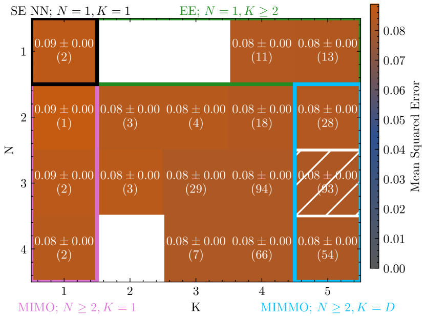
(a) MSE on RetinaMNIST OOD.

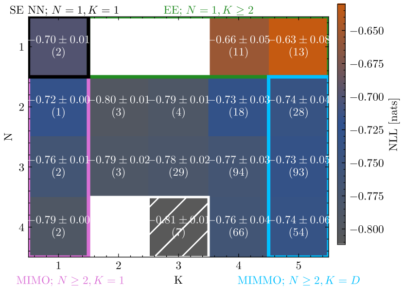
(b) NLL on RetinaMNIST OOD.

Figure 10: Varying $N,K$ on RetinaMNIST OOD test sets. The upper number is the average performance over $N$, $K$ combinations. The number in brackets is the number of sampled configurations by HPO. White box means no configurations sampled for that $N$, $K$. Pattern signals best average performance. The coloured outlines signal the special cases for the generalised methods.

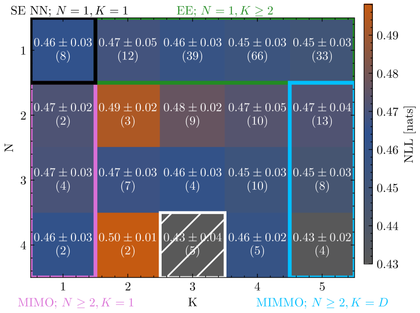
(a) NLL on PneumoniaMNIST ID.

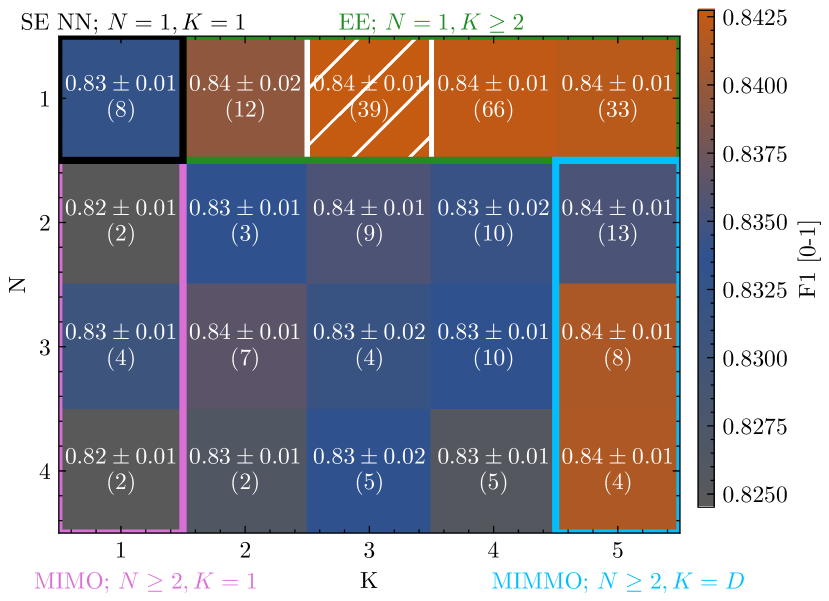
(b) F1 on PneumoniaMNIST ID.

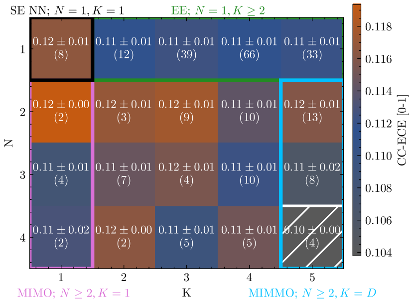
(c) ECE on PneumoniaMNIST ID.

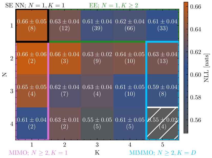
(d) NLL on PneumoniaMNIST OOD.

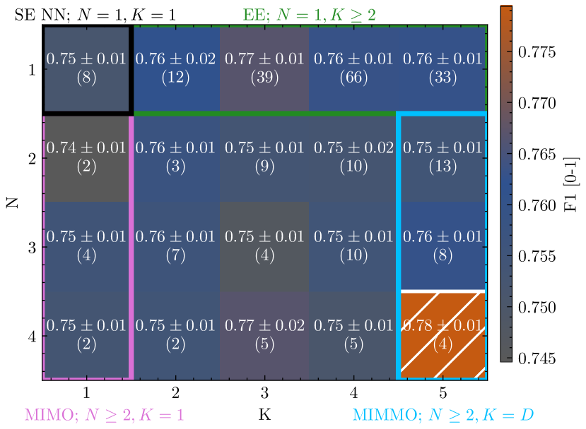
(e) F1 on PneumoniaMNIST OOD.

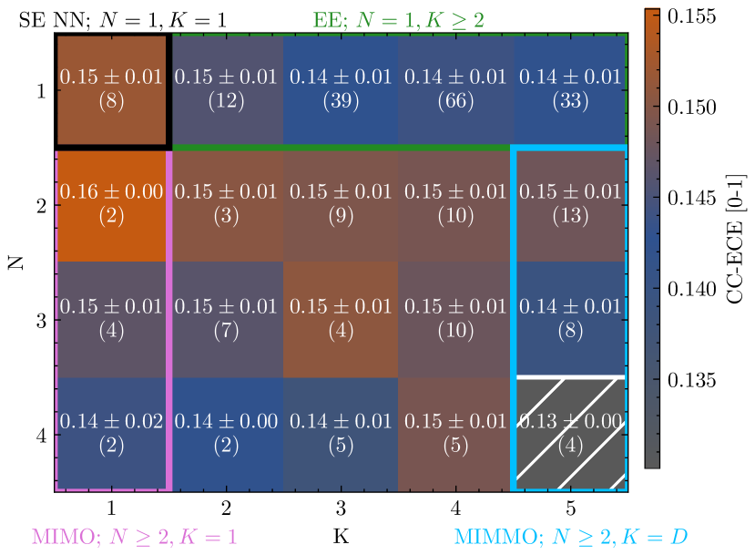
(f) ECE on PneumoniaMNIST OOD.

Figure 11: Varying $N,K$ on PneumoniaMNIST ID and OOD test sets. The upper number is the average performance over $N$, $K$ combinations. The number in brackets is the number of sampled configurations by HPO. White box means no configurations sampled for that $N$, $K$. Pattern signals best average performance. The coloured outlines signal the special cases for the generalised methods.

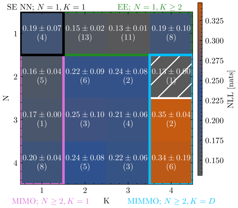
(a) NLL on BloodMNIST ID.

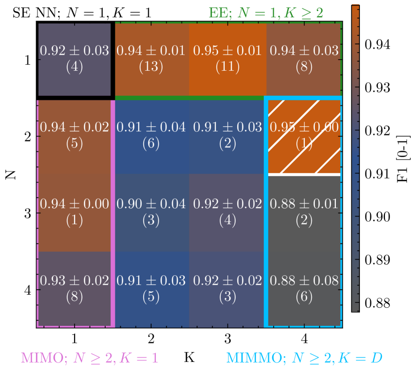
(b) F1 on BloodMNIST ID.

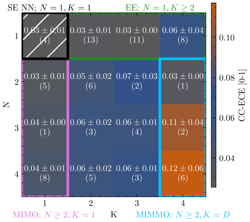
(c) ECE on BloodMNIST ID.

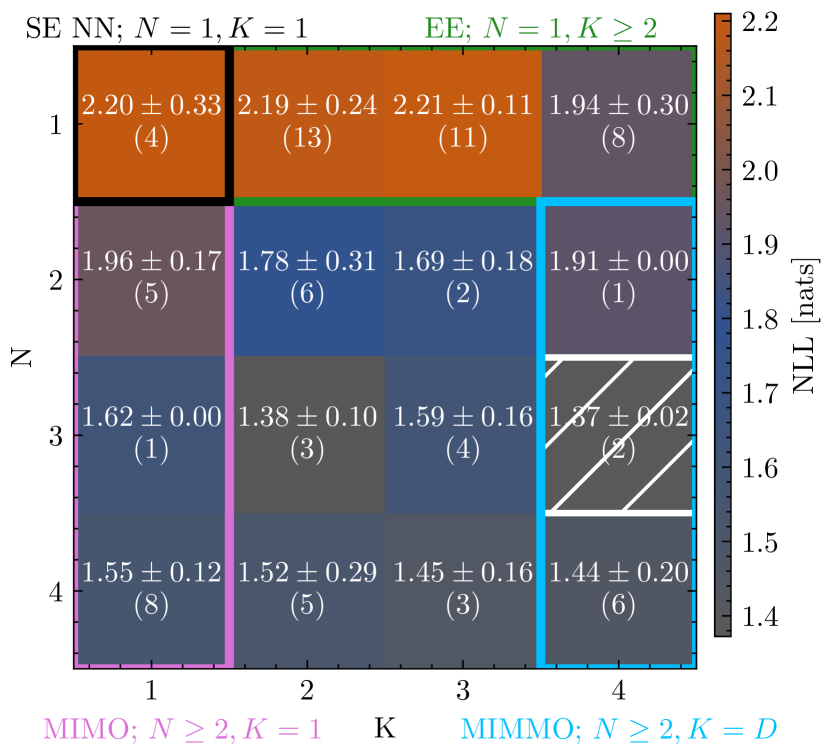
(d) NLL on BloodMNIST OOD.

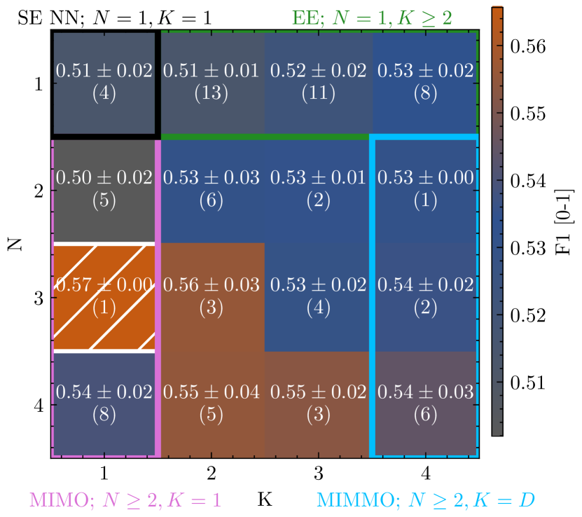
(e) F1 on BloodMNIST OOD.

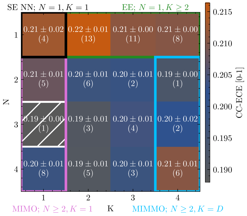
(f) ECE on BloodMNIST OOD.

Figure 12: Varying $N,K$ on BloodMNIST ID and OOD test sets. The upper number is the average performance over $N$, $K$ combinations. The number in brackets is the number of sampled configurations by HPO. White box means no configurations sampled for that $N$, $K$. Pattern signals best average performance. The coloured outlines signal the special cases for the generalised methods.

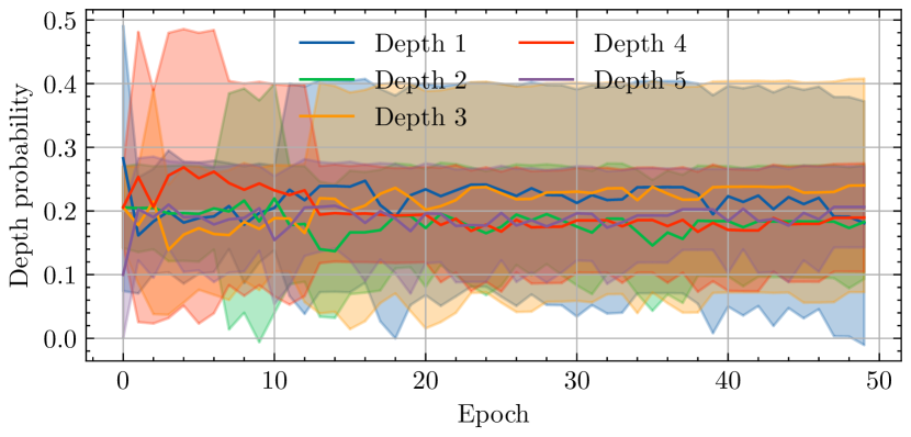
(a) $N=1$.

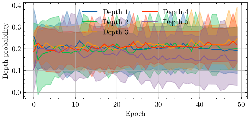
(b) $N=2$.

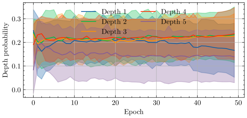
(c) $N=3$.

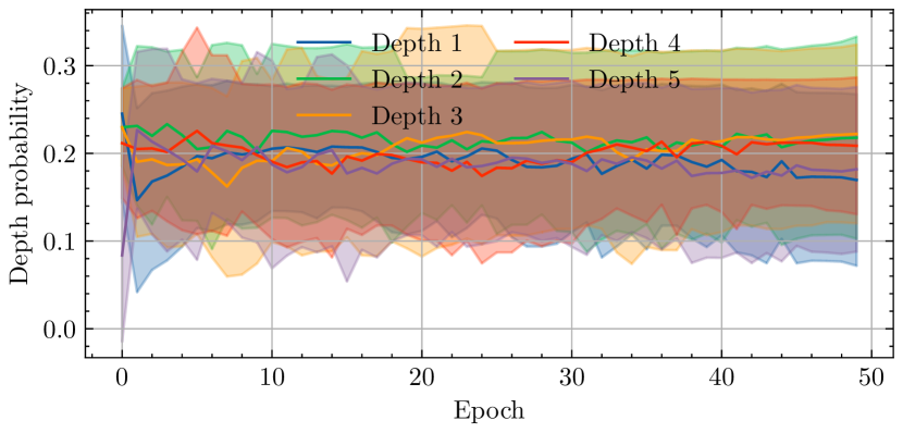
(d) $N=4$.

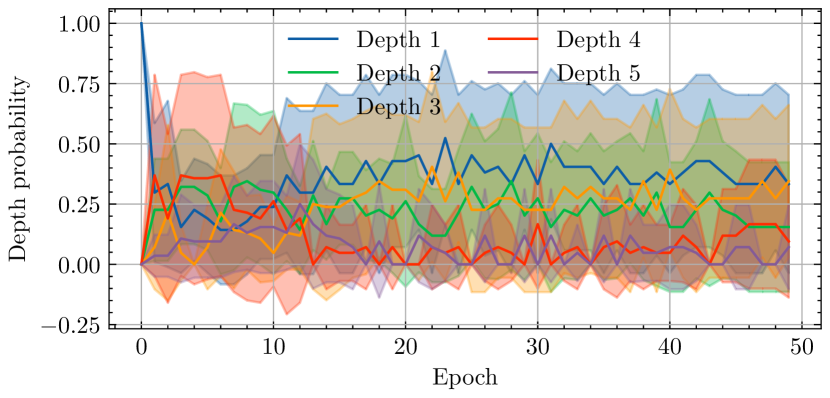
(e) $K=1$.

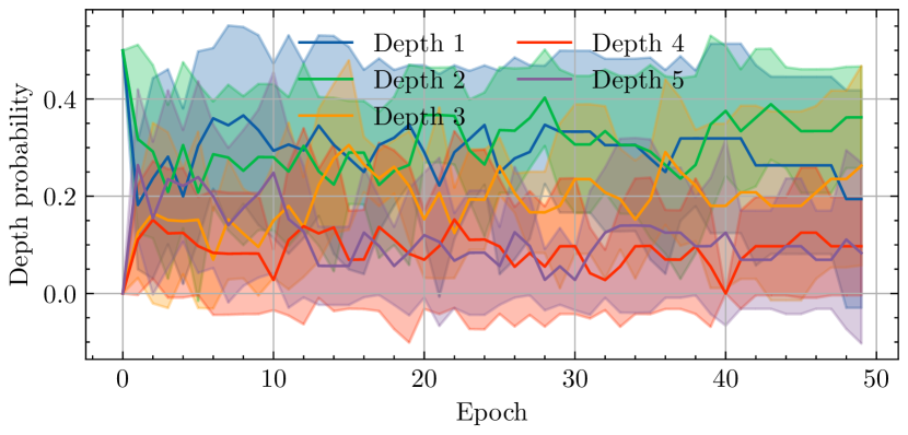
(f) $K=2$.

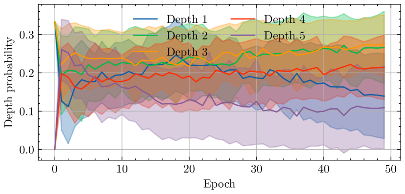
(g) $K=3$.

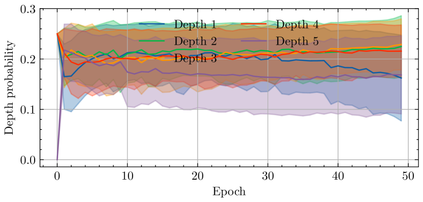
(h) $K=4$.

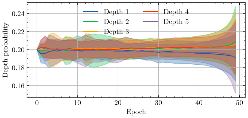
(i) $K=D$.

Figure 14: Depth preference during training when averaging over different $N$ and $K$ for RetinaMNIST. The lines denote the mean trend, and the shaded regions denote the standard deviation across configurations.

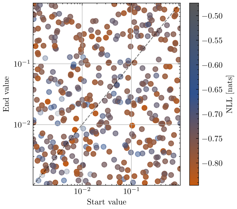
(a) Temperature for RetinaMNIST OOD.

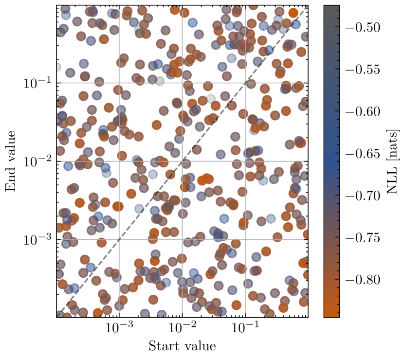
(b) Alpha for RetinaMNIST OOD.

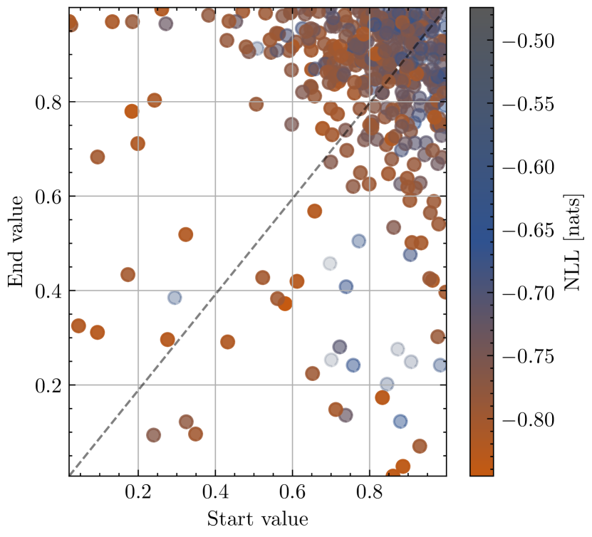
(c) Input repetition probability for RetinaMNIST OOD.

Figure 18: HP tuning for RetinaMNIST NLL on OOD test sets.

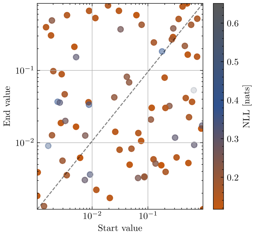
(a) Temperature for BloodMNIST ID.

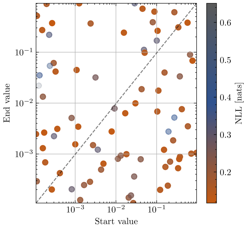
(b) Alpha for BloodMNIST ID.

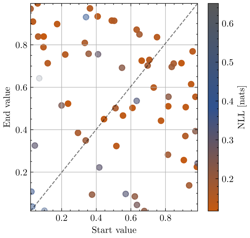
(c) Input repetition probability for BloodMNIST ID.

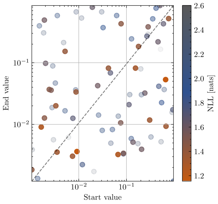
(d) Temperature for BloodMNIST OOD.

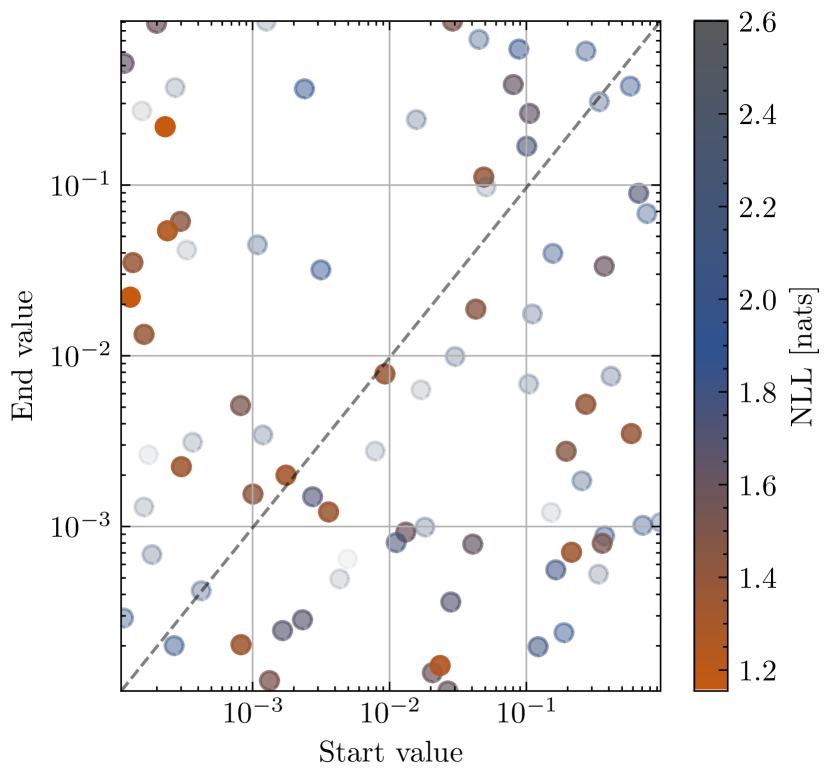
(e) Alpha for BloodMNIST OOD.

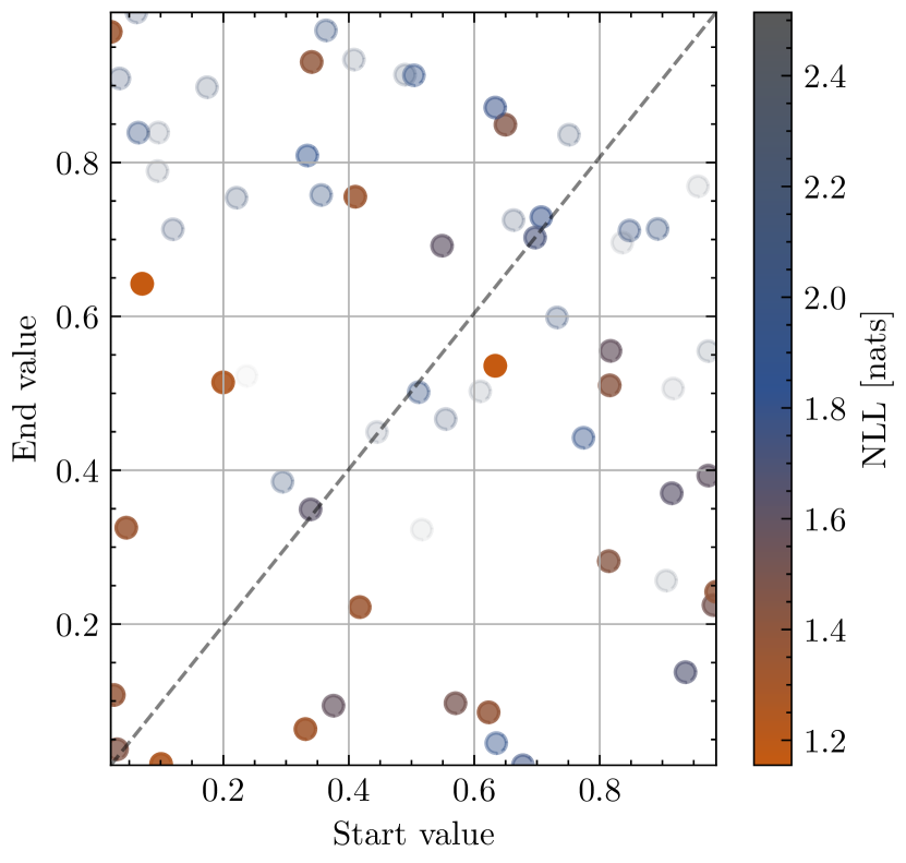
(f) Input repetition probability for BloodMNIST OOD.

Figure 19: HP tuning for BloodMNIST NLL on ID and OOD test sets.

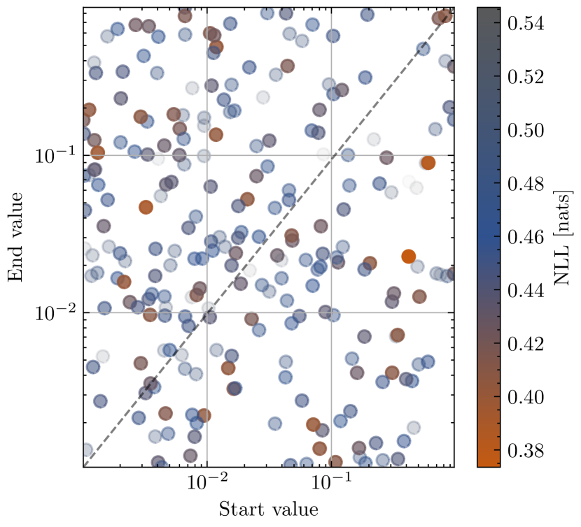
(a) Temperature for PneumoniaMNIST ID.

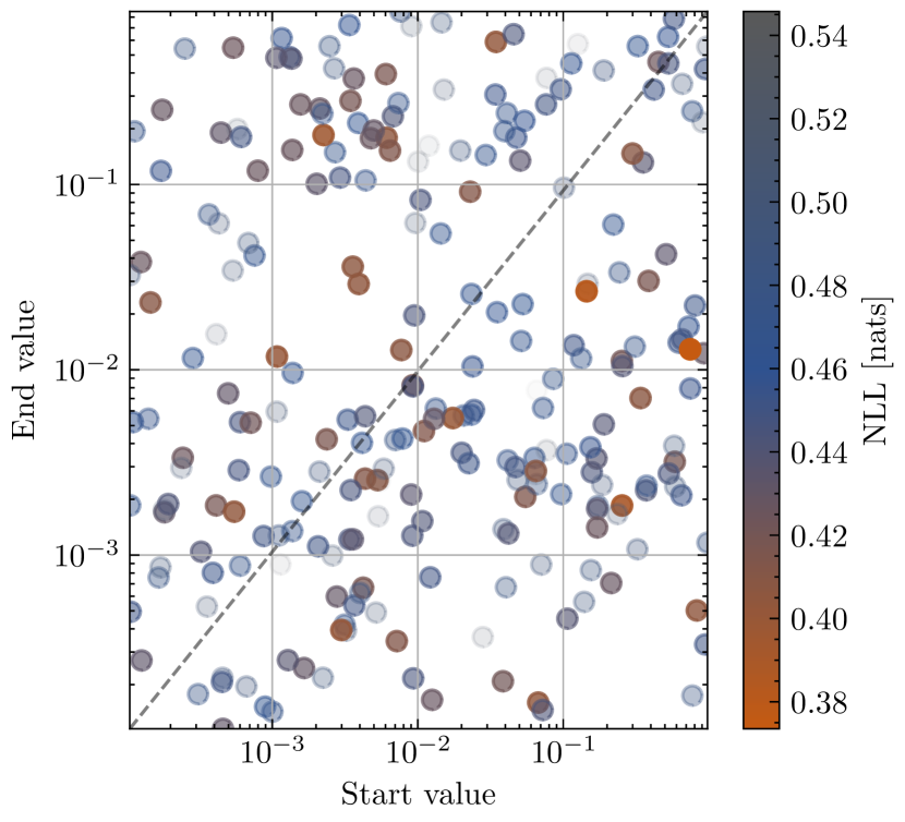
(b) Alpha for PneumoniaMNIST ID.

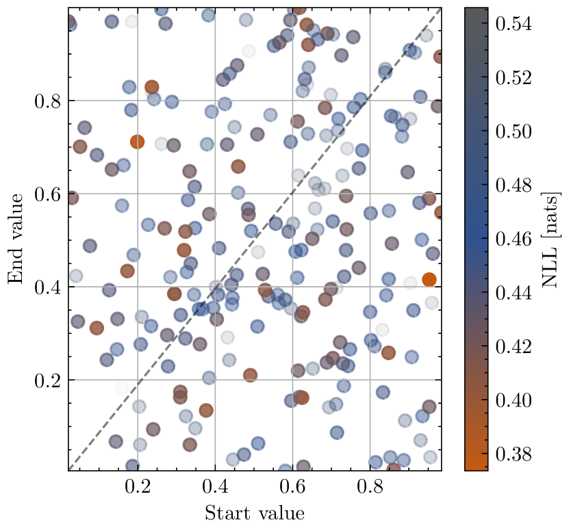
(c) Input repetition probability for PneumoniaMNIST ID.

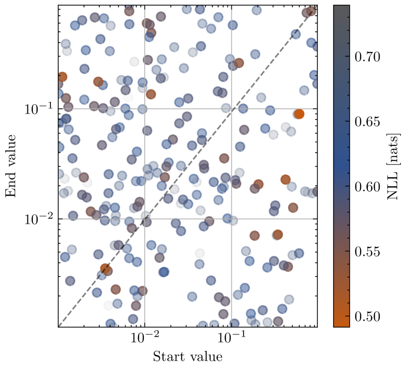
(d) Temperature for PneumoniaMNIST OOD.

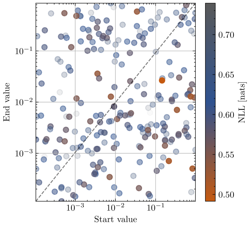
(e) Alpha for PneumoniaMNIST OOD.

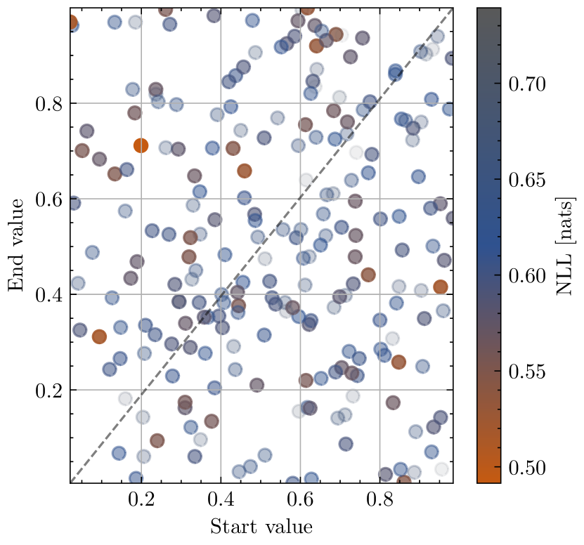
(f) Input repetition probability for PneumoniaMNIST OOD.

Figure 20: HP tuning for PneumoniaMNIST NLL on ID and OOD test sets.