On the Universality of Coupling-based Normalizing Flows

Abstract

We present a novel theoretical framework for understanding the expressive power of coupling-based normalizing flows such as RealNVP (Dinh et al., 2017). Despite their prevalence in scientific applications, a comprehensive understanding of coupling flows remains elusive due to their restricted architectures. Existing theorems fall short as they require the use of arbitrarily ill-conditioned neural networks, limiting practical applicability. Additionally, we demonstrate that these constructions inherently lead to volume-preserving flows, a property which we show to be a fundamental constraint for expressivity. We propose a new distributional universality theorem for coupling-based normalizing flows, which overcomes several limitations of prior work. Our results support the general wisdom that the coupling architecture is expressive and provide a nuanced view for choosing the expressivity of coupling functions, bridging a gap between empirical results and theoretical understanding.

1 Introduction

Density estimation and generative modeling of complex distributions is a fundamental problem in statistics and machine learning, with applications ranging from computer vision (Rombach et al., 2022) to molecule generation (Hoogeboom et al., 2022) and uncertainty quantification (Ardizzone et al., 2018b).

Normalizing flows are a common class of generative models that model a probability density which can be trained from samples via the maximum likelihood criterion. They are implemented by transporting a simple multivariate base density such as the standard normal via a learned invertible function to the distribution of interest. One particularly efficient variant of such invertible neural networks are based on so-called couplings blocks, which make the resulting distribution both fast to evaluate $p_{\theta}(x)\approx p(x)$ and sample from $x\sim p_{\theta}(x)\approx x\sim p(x)$.

Coupling blocks impose a strong architectural constraint on invertible neural networks. Most strikingly, half of the dimensions are left unchanged in each block, and the transformation of the remaining dimensions is restricted in order to ensure invertibility. At the same time, even the simple affine coupling-based normalizing flows can learn high-dimensional distributions such as images (Kingma & Dhariwal, 2018).

Theoretical explanations for this architecture’s ability to fit complex distributions are limited. Existing proofs make assumptions that are not valid in practice, as the involved constructions rely on ill-conditioned neural networks (Koehler et al., 2021).

We extend the theory in two ways: First, we prove that volume-preserving normalizing flows (Dinh et al., 2015; Sorrenson et al., 2019) are not universal approximators in terms of KL divergence, the practical loss measure. In fact, the existing universal approximation theorems for coupling-based normalizing flows construct volume-preserving flows (Teshima et al., 2020a; Koehler et al., 2021), fundamentally limiting their practical implications for learning distributions. Second, we introduce a new proof for the distributional universality of coupling-based normalizing flows. This proof is constructive, showing that training layers sequentially converges to the correct target distribution, which we illustrate in Figure 1.

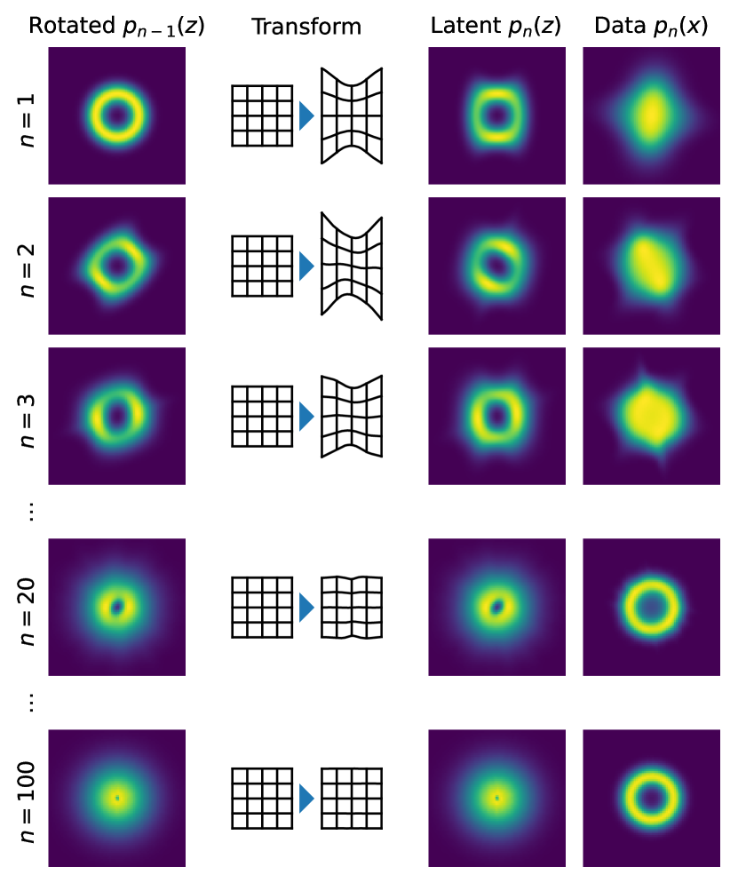
Figure 1: Our universality proof constructs a normalizing flow by iteratively adding affine coupling blocks. We illustrate this by constructing such a flow from real data. Each block first rotates the distribution $p_{n-1}(z)$ from the previous step (first column), then applies an affine coupling layer that transforms the active dimensions to zero mean and unit variance for each passive coordinate $b$ (second column). The resulting latent distribution converges step by step (third column) to a standard normal distribution, where the learned additional layers essentially learn the identity (last row). The data distribution $p_{\theta}(x)$ converges in parallel (right).

In summary, we contribute:

• We show the limits of volume-preserving flows as distributional universal approximator in Section 4.2.

• We then show that existing distributional universality proofs for affine coupling-based normalizing flows construct such volume-preserving flows in Section 4.3.

• We give a new universality proof for coupling-based normalizing flows that overcomes previous shortcomings in Section 4.5.

Our results validate a crucial insight previously observed only empirically: Affine coupling blocks are an effective foundation for normalizing flows. Our proof elucidates how more expressive coupling functions can achieve good performance with fewer layers. Additionally, our findings advise caution in using volume-preserving flows due to their inherent limitations in expressivity.

2 Related Work

Normalizing flows form a class of generative models that are based on invertible neural networks (Rezende & Mohamed, 2015). We focus on the widely-used coupling-based flows, which involve a sequence of simple invertible blocks (Dinh et al. (2015, 2017), see Section 3).

That coupling-based normalizing flows work well in practice despite their restricted architecture has sparked the interest of several papers analyzing their distributional universality, i.e. the question whether they can approximate any target distribution to arbitrary precision (see Definition 4.1). Teshima et al. (2020a) showed that that coupling flows are universal approximators for invertible functions, which results in distributional universality. Koehler et al. (2021) demonstrated that affine coupling-based normalizing flows can approximate any distribution with arbitrary precision using just three coupling blocks. However, these works assume neural networks with exploding derivatives for couplings, an unrealistic condition in practical scenarios. Our work addresses this limitation by showing that training a normalizing flow layer by layer yields universality. We additionally demonstrate that these works construct volume-preserving transformations in Section 4.3, an additional important limitation.

Some works show distributional universality of augmented affine coupling-based normalizing flows, which add at least one additional dimension usually filled with exact zeros (Huang et al., 2020; Koehler et al., 2021; Lyu et al., 2022). The problem with adding additional zeros is that the flow is not exactly invertible anymore in the data domain and usually loses tractability of the change of variables formula (Equation 1). Lee et al. (2021) add i.i.d. Gaussians as additional dimensions, which again allows density estimation, but they only show how to approximate the limited class of log-concave distributions. Our universality proof does not rely on such a construction.

Other theoretical work on the expressivity of normalizing flows considers more expressive invertible neural networks, including SoS polynomial flows, Neural ODEs and Residual Neural Networks (Jaini et al., 2019; Zhang et al., 2020; Teshima et al., 2020b; Ishikawa et al., 2022). Another line of work found that the number of required coupling blocks is independent of dimension $D$ for Gaussian distributions compared to $O(D)$ Gaussianization blocks that lack couplings between dimensions (Koehler et al., 2021; Draxler et al., 2022, 2023).

3 Coupling-based Normalizing Flows

Normalizing Flows are a class of generative models that represent a distribution $p_{\theta}(x)$ with parameters $\theta$ by learning an invertible function $z=f_{\theta}(x)$ so that distribution of the latent codes $z\in\mathbb{R}^{D}$ obtained from the data $x\in\mathbb{R}^{D}$ are distributed like a standard normal distribution $p(z)=\mathcal{N}(z;0,I)$. Via the change of variables formula, see (Köthe, 2023) for a review, this invertible function yields an explicit form for the density $p_{\theta}(x)$:

$$p_{\theta}(x)=p(z=f_{\theta}(x))|f_{\theta}^{\prime}(x)|,$$ (1)

where $f_{\theta}^{\prime}(x)=\frac{\partial}{\partial x}f_{\theta}(x)$ is the Jacobian matrix of $f_{\theta}$ at $x$ and $|f_{\theta}^{\prime}(x)|$ is its absolute determinant.

Equation 1 allows easily evaluating the model density at points of interest. Obtaining samples from $p_{\theta}(x)$ can be achieved by sampling from the latent standard normal and applying the inverse $f_{\theta}^{-1}(z)$ of the learned transformation:

$$x=f_{\theta}^{-1}(z)\sim p_{\theta}(x)\text{ for }z\sim p(z).$$ (2)

The change of variables formula (Equation 1) can be used directly to train a normalizing flow. The corresponding loss minimizes the Kullback-Leibler divergence between the true data distribution $p(x)$ and the learned distribution, which can be optimized via a Monte-Carlo estimate of the involved expectation:

$$\mathcal{L} =\mathcal{D}_{\text{KL}}(p(x)\|p_{\theta}(x))$$ (3)

$$=\mathbb{E}_{x\sim p(x)}[\log p(x)-\log p_{\theta}(x)]$$ (4)

$$=\mathbb{E}_{x\sim p(x)}[-\log p_{\theta}(x)]+\text{const.}$$ (5)

This last variant makes clear that minimizing this loss is exactly the same as maximizing the log-likelihood of the training data. For training, the expectation value is approximated using (batches of) training samples $x_{1,\dots,N}$.

In order for Equations 1 and 2 to be useful in practice, $f_{\theta}(x)$ must have (i) a tractable inverse $f_{\theta}^{-1}(z)$ for fast sampling, and (ii) a tractable Jacobian determinant $|f_{\theta}^{\prime}(x)|$ for fast training while (iii) being expressive enough to model complicated distributions. These constraints are nontrivial to fulfill at the same time and significant work has been put into constructing such invertible neural networks.

In this work, we focus on the class of coupling-based neural networks (Dinh et al., 2015, 2017). This design lies in a sweet spot of being expressive yet easy to invert (Draxler et al., 2023) and exhibits a tractable Jacobian determinant. Its basic building block is the coupling layer, which consists of one invertible function $\tilde{x}_{i}=c(x_{i};\theta_{i})$ for each dimension, but with a twist: Only the second half of the dimensions $a=x_{D/2+1,\dots,D}$ (active) is changed in a coupling layer, and the parameters $\theta=\theta(b)$ are predicted by a neural network that depends on the first half of dimensions $b=x_{1,\dots,D/2}$ (passive):

$$\tilde{x}=f_{\text{cpl}}(x)=\begin{pmatrix}b_{1}\\ \vdots\\ b_{D/2}\\ c(a_{1};\theta_{1}(b))\\ \vdots\\ c(a_{D/2};\theta_{D}(b))\end{pmatrix}.$$ (6)

The neural network $\theta(b)$ allows for modeling dependencies between dimensions in the coupling layer. Calculating the inverse of the coupling layer is easy, as $b=\tilde{b}$ for the passive dimensions. This allows computing the parameters $\theta(b)$ necessary to invert the active half of dimensions:

$$x=f_{\text{cpl}}^{-1}(\tilde{x})=\begin{pmatrix}\tilde{b}_{1}\\ \vdots\\ \tilde{b}_{D/2}\\ c^{-1}(a_{1}^{\prime};\theta_{1}(\tilde{b}))\\ \vdots\\ c^{-1}(a_{D/2}^{\prime};\theta_{D/2}(\tilde{b}))\end{pmatrix}.$$ (7)

Choosing the right one-dimensional invertible function $c(x;\theta)$ is the subject of active research, see our list in Appendix A and the review by Kobyzev et al. (2021). Many applications use affine-linear functions $c(x;s,t)=sx+t$ where $s>0$ and $t$ are the parameters to be predicted by the $\theta(b)$ subnetwork as a function of the passive dimensions. Especially for smaller-dimensional problems it has proven useful to use more flexible $c$ such as rational-quadratic splines (Durkan et al., 2019b). Our universality results are compatible with all coupling architectures we are aware of except for NICE. At the same time, our construction gives a direct reason for using more expressive couplings, as they can learn the same distributions with fewer layers (see Section 4.6).

In order to be expressive, a normalizing flow consists of a stack of coupling layers, each with a different active and passive subspace. This is realized by an additional layer before each coupling which rotates an incoming vector $x$ via a rotation matrix $Q\in SO(D)$:

$$f_{\text{rot}}(x) =Qx,$$ (8)

$$f_{\text{rot}}^{-1}(\tilde{x}) =Q^{T}\tilde{x}.$$ (9)

Often, $Q$ is simply chosen as a permutation matrix that is fixed during training, but some variants allow any rotation $Q$ or learning the rotation during training (Kingma & Dhariwal, 2018). Our universality theorem will consider free-form rotation matrices $Q$. This does not restrict its applicability to some architectures, since any invertible linear function can be represented by a fixed number of coupling blocks with fixed permutations (Koehler et al., 2021).

A rotation layer together with a coupling layer forms a coupling block:

$$f_{\text{blk}}(x)=(f_{\text{cpl}}\circ f_{\text{rot}})(x)=f_{\text{cpl}}(Qx).$$ (10)

In the remainder of this paper, we are concerned with what distributions $p(x)$ a potentially deep concatenation of coupling blocks can represent.

4 Distributional Universality of Coupling Flows

In this section, we give our new distributional universality results for coupling-based normalizing flows. We start off by explaining what we mean by distributional universality. We then show a negative result concerning volume-preserving flows, in that they are not distributional universal approximator in terms of KL divergence. This shows a fundamental limitation of previous universality proofs of coupling flows. We then give our proof that overcomes several of those shortcomings.

4.1 Distributional Universality

By distributional universality we mean that a certain class of generative models can represent any distribution $p(x)$. Due to the nature of neural networks, we cannot hope for our generative model to exactly (i.e. exact equality in the mathematical sense) represent $p(x)$. This becomes clear via an analogue in the context of regression: A neural network with ReLU activations always models piecewise linear functions, and as such it can never exactly regress a parabola $y=x^{2}$. However, for every finite value of $\epsilon>0$ and given more and more linear pieces, it can follow the parabola ever so closer, so that the average distance between $x^{2}$ and $f_{\theta}(x)$ vanishes: $\mathbb{E}_{x\sim p(x)}[|x^{2}-f_{\theta}(x)|^{2}]<\epsilon$. To characterize the expressivity of a class of neural networks, it is thus instructive to call a class of networks universal if the error between the model and any target can be reduced arbitrarily.

In terms of representing distributions $p(x)$, the following definition captures universality of a class of model distributions, similar to (Teshima et al., 2020a, Definition 3):

Definition 4.1.

A set of probability distributions $\mathcal{P}$ is called a distributional universal approximator if for every possible target distribution $p(x)$ there is a sequence of distributions $p_{n}(x)\in\mathcal{P}$ such that $p_{n}(x)\xrightarrow{n\to\infty}p(x)$.

The formulation of universality as a convergent series is useful as it (i) captures that the distribution in question $p(x)$ may not lie in $\mathcal{P}$, and (ii) the series index $n$ usually reflects a hyperparameter of the underlying model corresponding to computational requirements (for example, the depth of the network).

We have left the exact definition of the limit “$p_{n}(x)\xrightarrow{n\to\infty}$ p(x)” open as we may want to consider different variations of convergence. The existing literature on affine coupling-based normalizing flows considers weak convergence (Teshima et al., 2020a) respectively convergence in Wasserstein distance (Koehler et al., 2021). We will note in Section 4.3 that the constructions used in the existing proofs are fundamentally tied to these relatively weak convergence metrics. Many metrics of convergence have been proposed, see (Gibbs & Su, 2002) for a systematic overview.

In this paper, we consider continuous target distributions $p(x)$ that have infinite support and finite moments, which covers distributions of practical interest.

4.2 Limitations of Volume-preserving Flows

In this section, we provide a negative universality result of normalizing flows which have a constant Jacobian determinant $|f_{\theta}^{\prime}(x)|=\operatorname{const}$, such as nonlinear independent components estimation (NICE) (Dinh et al., 2015) or general incompressible-flow networks (GIN) (Sorrenson et al., 2019). Such flows are usually called volume-preserving flows or sometimes incompressible flows.

For one-dimensional functions, this implies that $f_{\theta}(x)$ is linear. For multivariate functions, $f_{\theta}(x)$ can be nonlinear, only that any volume change in one dimension must be compensated by an inverse volume change in the remaining dimensions. For example, GIN realizes volume-preserving coupling blocks by requiring that $\sum_{i=1}^{D/2}\log s_{i}(b)=\operatorname{const}$. This is more expressive than NICE, which set all $s_{i}(b)=1$ except in a linear rescaling layer.

While volume-preserving flows can be useful in certain applications such as disentanglement (Sorrenson et al., 2019) or temperature-scaling in Boltzmann generators (Dibak et al., 2022), they are at disadvantage in terms of what distributions they can learn.

To derive this, let us adapt the change of variables formula Equation 1 to volume-preserving flows:

$$p_{\theta}(x)=p(z=f_{\theta}(x))C,$$ (11)

where $C=|f_{\theta}^{\prime}(x)|$. This equation says that for every $x$ the density modeled by the flow is exactly the density of the corresponding latent code $z=f_{\theta}(x)$ up to a constant factor – and likewise every latent code must lend its relative likelihood to exactly one point in the data space.

It turns out that this restriction is fatal for the expressivity of volume-preserving flows:

Theorem 4.2.

The family of normalizing flows with constant Jacobian determinant $|f_{\theta}^{\prime}(x)|=\operatorname{const}$ is not a universal distribution approximator under KL divergence.

In the detailed proof in Section B.1, we construct a counter-example of a distribution that cannot be approximated in terms of KL divergence. Intuitively speaking, volume-preserving flows can only morph the latent distribution $p(z)$ by shifting regions of it around, but they cannot compress or inflate space to vary the local density by Equation 11. This implies that the structure of $p_{\theta}(x)$ is essentially shared with the latent distribution $p(z)$. For example, the local maxima of the learned density, usually referred to as its modes, are inherited from the latent distribution. This means that the learned distribution cannot create multi-modal distributions from a standard normal latent space:

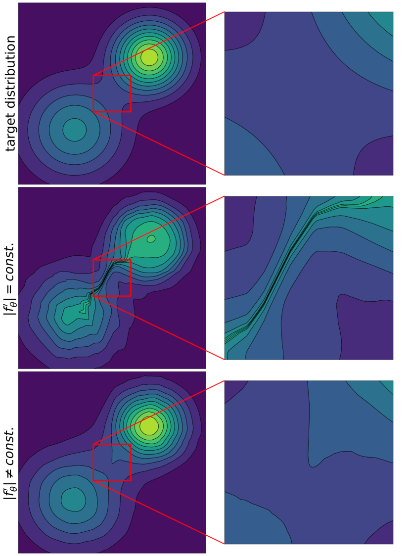
Figure 2: A normalizing flow with constant Jacobian determinant is not able to model a simple bimodal mixture (first vs second row): The modeled density in both modes is almost identical despite their different weight in the ground truth. Also, the volume-preserving flow really has only one maximum and the second pseudo mode is connected to the first by a bridge of high density. A normalizing flow with variable Jacobin determinant does not have these issues (third row).

Corollary 4.3.

A normalizing flow $p_{\theta}(x)$ with constant Jacobian determinant $|f_{\theta}^{\prime}(x)|=\operatorname{const}$ has the same number of modes as the latent distribution $p(z)$.

Figure 2 illustrates this shortcoming by learning a two-dimensional target distribution with an volume-preserving flow. The problem is that by Equation 11 there is a one-to-one correspondence between maxima of $p_{\theta}(x)$ and $p(z)$ and the neighborhoods in data and latent space. In the example, this connects the learned “modes” by a thin bridge and they really form one connected region of high probability without a barrier. In addition, the density is off at both modes. A normalizing flow with flexible volume change does not have these issues and correctly approximates the bimodal distribution. We give the detailed proof in Section B.2 and experimental details in Section E.2.

This can partially be recovered by having a (learnable) multi-modal distribution in the latent space, but this is necessarily limited if the structure of the distribution to learn is unknown.

Our Theorems 4.2 and 4.3 identify a fundamental limitation for applications based on volume-preserving flows. It explains why RealNVP significantly outperforms NICE in practice (Dinh et al., 2017). Work using volume-preserving flows must take this limited expressivity and the resulting biases in the learned distributions into account. In the next section, we will find that this problem also applies in existing universality proofs for coupling-based normalizing flows.

4.3 Problems with Existing Constructions

There are already existing proofs showing that affine and more expressive coupling flows are distributional universal approximators. They make use of specially parameterized coupling blocks that results in convergence to arbitrary distributions (Teshima et al., 2020a; Koehler et al., 2021). While technically correct, the metrics of convergence employed by (Teshima et al., 2020a; Koehler et al., 2021) are indifferent to two shortcomings of these constructions: they require ill-conditioned networks and construct volume-preserving flows, which are not universal in KL divergence by our Theorem 4.2. We will demonstrate the shortcomings via the approach presented in Koehler et al. (2021), but the same arguments also apply to the construction in (Teshima et al., 2020a).

The key result in Koehler et al. (2021, Theorem 1) is that for any approximation error $\epsilon>0$ it is possible to construct a coupling flow $f_{\theta}$ consisting of three affine couplings blocks for which the Wasserstein distance $W_{2}$ is smaller than $\epsilon$:

$$W_{2}(p_{\theta}(x),p(x))<\epsilon.$$ (12)

In the proof of this statement explicit formulas for the rotations, offset and scaling functions in the three affine coupling layers are given. To make our point, let us take a closer look at the scaling terms $s(b)$ of the affine couplings $\tilde{a}=s(b)\odot a+t(b)$. For the three affine coupling layers the scaling factors are given by $s_{1}=\epsilon^{\prime}$ and $s_{2}=s_{3}=\epsilon^{\prime\prime}$ for each active dimension where $\epsilon^{\prime}$ and $\epsilon^{\prime\prime}$ are two constants smaller than $\epsilon$. Computing the network’s Jacobian determinant we find $\mathopen{}\mathclose{{}\left|f^{-1\prime}_{\theta}}\right|=\mathopen{}\mathclose{{}\left(\epsilon^{\prime}\cdot\epsilon^{\prime\prime}\cdot\epsilon^{\prime\prime}}\right)^{\frac{D}{2}}$ and $\mathopen{}\mathclose{{}\left|f^{\prime}_{\theta}}\right|=\mathopen{}\mathclose{{}\left(\epsilon^{\prime}\cdot\epsilon^{\prime\prime}\cdot\epsilon^{\prime\prime}}\right)^{-\frac{D}{2}}$.

The derived expressions for Jacobian determinants show two important shortcomings for the universality theorems. The first one is that as the approximation error $\epsilon$ becomes very small, $\epsilon^{\prime}$ and $\epsilon^{\prime\prime}$ also becomes very small. For the forward pass this leads to a vanishing and for the inverse pass to an exploding Jacobian determinant. This illustrates the point made in Koehler et al. (2021, Remark 2) that for small approximation errors, the network is ill-conditioned, making the construction unrealistic.

The second point is a more fundamental issue. The derived expressions for the Jacobian determinants of the normalizing flow with the constructed parameters for the three affine couplings as given in (Koehler et al., 2021) show that these determinants are constant as $\epsilon^{\prime}$ and $\epsilon^{\prime\prime}$ are constant factors. The resulting construction is therefore a volume-preserving flow, which we considered in the previous section. This means that by our Theorems 4.2 and 4.3, the resulting normalizing flows are not distributional universal approximators under KL divergence and always represent unimodal distributions regardless of the data distribution.

The insights from this section, that existing constructions rely on ill-conditioned normalizing flows and do not converge under KL divergence, motivate the introduction of our new universality theorem.

4.4 Convergence Metric

Ideally, we would make a universality statement in terms of the KL divergence in Equation 3 as our measure of convergence. It is not only the metric used in practice, it also a strong metric of convergence that implies weak convergence, that ensures convergence of expectation values, and it implies convergence of the densities (Gibbs & Su, 2002). Also, as we showed previously in Section 4.2, the KL divergence is able to distinguish the expressivity between volume-preserving and non-volume-preserving flows, but weak convergence and Wasserstein distance are not (Section 4.3).

The metric of convergence we consider in our proof is indeed related to the Kullback-Leibler divergence. To construct it, rewrite the loss $\mathcal{L}$ in Equation 3 in comparing the current latent distribution $p_{\theta}(z)$ as the push forward of $p(x)$ through our flow $f_{\theta}(x)$:

$$\mathcal{L} =\mathcal{D}_{\text{KL}}(p(x)\|p_{\theta}(x))$$ (13)

$$=\int p(x)\log\frac{p(x)}{p(z=f(x))|f^{\prime}(x)|}dx$$ (14)

$$=\int p(z)|f_{\theta}^{-1}{}^{\prime}(z)|\log\frac{p(f^{-1}(z))|f_{\theta}^{-1}{}^{\prime}(z)|}{p(z)}dz$$ (15)

$$=\mathcal{D}_{\text{KL}}(p_{\theta}(z)\|p(z)).$$ (16)

This identity shows that the divergence between the true $p(x)$ and the model $p_{\theta}(x)$ can equally be measured in the latent space, via the KL divergence between the current latent distribution that the model generates from the data $p_{\theta}(z)$ and the target latent distribution $p(z)$.

Let us now consider what happens if we append one more affine coupling block to an existing normalizing flow $f_{\theta}(x)$, resulting in a flow which we call $p_{\theta\cup\varphi}(x)$. Let us choose the parameters of the additional coupling block $\varphi$ such that it maximally reduces the loss without changing the previous parameters:

$$\min_{\varphi}\mathcal{D}_{\text{KL}}(p_{\theta\cup\varphi}(z)\|p(z)).$$ (17)

This allows us to measure the additional loss improvement that was achieved by adding one more affine coupling block:

$$\Delta_{\textnormal{affine}}:=\min_{\varphi}\mathcal{D}_{\text{KL}}(p_{\theta\cup\varphi}(z)\|p(z))-\mathcal{D}_{\text{KL}}(p_{\theta}(z)\|p(z)).$$ (18)

Note that for our argument it is sufficient to consider affine coupling blocks, but the results extend to more expressive coupling functions as well.

The following theorem allows us to use the above loss improvement $\Delta_{\textnormal{affine}}$ as a convergence metric for distributions. It states that adding another coupling layer can always improve on the loss $\mathcal{L}$ unless it has already converged to a standard normal in the latent space:

Theorem 4.4.

Let $p(z)$ be a continuous probability distribution with finite first and second moment and $p(x)>0$ for all $x\in RR^{D}$. Then, the distribution is the standard normal distribution if and only if an affine coupling block with a ReLU subnetwork $\theta(x_{1,\dots,D/2})$ containing at list two hidden layers cannot improve the KL divergence as given by Equation 18:

$$p(z)=\mathcal{N}(z;0,I)\Leftrightarrow\Delta_{\textnormal{affine}}=0.$$ (19)

This shows that the maximally achievable loss improvement $\Delta_{\textnormal{affine}}$ is a useful convergence metric for normalizing flows: If adding more layers has no effect then the latent distribution has converged to the right distribution.

In the remainder of this section, we give a sketch of the proof of Theorem 4.4, with technical details moved to Section C.1. We will continue with our universality theorem in the next section.

We proceed as follows: First, we use an explicit form of the maximal loss improvement $\Delta_{\textnormal{affine}}^{*}$ for infinitely expressive affine coupling blocks (Draxler et al., 2020). Then, we show in Lemma 4.5 that convergence of these unrealistic networks is equivalent to convergence of finite ReLU networks. Finally, we show that $\Delta_{\textnormal{affine}}=0$ implies $p(z)=\mathcal{N}(z;0,I)$. While this derivation is constructed for affine coupling blocks, it also holds for coupling functions which are more expressive (see Appendix A for all applicable couplings we are aware of): If an affine coupling block cannot make an improvement, neither can a more expressive coupling. The other direction is trivial, since by $p(z)=\mathcal{N}(0,I)$, no loss improvement is possible.

If we assume for a moment that neural networks can exactly represent arbitrary continuous functions, then this hypothetical maximal loss improvement was computed by Draxler et al. (2020, Theorem 1). A single affine coupling block with a fixed rotation layer $Q$, in order to maximally reduce the loss, will standardize the data by normalizing the first two moments of the active half of dimensions $a=(Qx)_{D/2+1,\dots,D}$ conditioned on the passive half of dimensions $b=(Qx)_{1,\dots,D}$. The moments before the coupling

$$\mathbb{E}_{a_{i}|b}[a_{i}] =m_{i}(b), \operatorname{Var}_{a_{i}|b}[a_{i}] =\sigma_{i}(b)$$ (20)

are mapped to:

$$\mathbb{E}_{\tilde{a}_{i}|b}[\tilde{a}_{i}] =0, \operatorname{Var}_{\tilde{a}_{i}|b}[\tilde{a}_{i}] =1.$$ (21)

This is achieved via the following affine transformation, shifting the mean to zero and scaling the standard deviation to one:

$$\tilde{a}_{i}(a_{i};b)=\frac{1}{\sigma_{i}(b)}(a_{i}-m_{i}(b)).$$ (22)

In terms of loss, this transformation can at most achieve the following loss improvement, with a contribution from each passive coordinate $b$:

$$\Delta_{\textnormal{affine}}^{*}=\max_{Q}\tfrac{1}{2}\sum_{i}^{D/2}\mathbb{E}_{b}\mathopen{}\mathclose{{}\left[m_{i}^{2}(b)+\sigma_{i}^{2}(b)-1-\log\sigma_{i}^{2}(b)}\right].$$ (23)

With the asterisk, we denote that this improvement can not necessarily be reached in practice with finite neural networks. More expressive coupling functions can reduce the loss stronger. We pick up on this point in Section 4.6.

What loss improvement can be achieved if we go back to finite neural networks? In the following statement, we show that $\Delta_{\textnormal{affine}}^{*}>0$ is equivalent to the existence of a two layer ReLU subnetwork with finite width which determines the parameters in an affine coupling block $f_{\text{cpl}}$ that achieves $\Delta_{\textnormal{affine}}>0$:

Lemma 4.5.

Given a continuous probability density $p(z)$ on $z\in\mathbb{R}^{k}$. Then,

$$\Delta_{\textnormal{affine}}^{*} >0$$ (24)

if and only if there is a ReLU neural network with two hidden layers with a finite number of neurons such that:

$$\Delta_{\textnormal{affine}} >0.$$ (25)

This says that the events $\Delta_{\textnormal{affine}}=0$ and $\Delta_{\textnormal{affine}}^{*}=0$ can be used interchangeably. The equivalence comes from the fact that if $\Delta_{\textnormal{affine}}>0$, then we can always construct a two-layer ReLU neural network that scales the conditional standard deviations closer to one and the conditional means closer to zero. In the detailed proof in Section C.1.2 we also make use of a classical regression universal approximation theorem (Hornik, 1991).

Finally, if the first two conditional moments of any latent distribution $p(z)$ are normalized for all rotations $Q$:

$$\mathbb{E}_{a_{i}|b}[a_{i}]=0,\quad\operatorname{Var}_{a_{i}|b}[a_{i}]=1,$$ (26)

then the distribution must be the standard normal distribution: $p(z)=\mathcal{N}(z;0,I)$. This can be obtained directly by combining Gaussian identification results (Eaton, 1986; Bryc, 1995).

This concludes the proof sketch of Theorem 4.4 and we are now ready to present our universality result, employing $\Delta_{\textnormal{affine}}$ as a convergence metric.

4.5 Affine Coupling Flows Universality

To construct our universal coupling flow, we follow a simple iterative scheme. We start with the data distribution as our original guess for the latent distribution: $p_{0}(z)=p(x=z)$. Then, we append a single affine coupling block $f_{\text{blk}}(x)$ consisting of a rotation $Q$ and a coupling $f_{\text{cpl}}$. We optimize the new parameters to maximally reduce the loss as in Equation 17 and get a new latent estimate $p_{1}(z)=p_{\varphi}(z)$.

The following theorem assures us that iterating this procedure makes the latent distribution $p_{n}(z)$ converge to the standard normal distribution in the latent space $p(z)$:

Theorem 4.6.

Coupling-based normalizing flows with affine couplings are distributional universal approximator under the convergence metric $\Delta_{\textnormal{affine}}$ as given in Section 4.4.

The proof idea is simple: The convergence metric $\Delta_{\textnormal{affine}}$ measures how much adding another affine coupling block can reduce the loss $\mathcal{L}$, but the total loss that can be reduced by the concatenation of many blocks is bounded. Thus, later layers cannot arbitrarily improve on the loss and their loss improvements $\Delta_{\textnormal{affine}}$ must converge to zero. By Theorem 4.4, the fixed point of this procedure has a standard normal distribution in the latent space. We give the full proof in Section C.2.

Figure 1 shows an example for how Theorem 4.6 constructs the coupling flow in order to learn a toy distribution. The affine coupling flow is able to learn the distribution well, despite the difficult topology of the problem.

While our proof removes spurious constructions present in previous work, there are still some properties we hope can be improved in the future: First, the construction does not exploit that a deep stack of blocks can undertake coordinated action, which can be found using end-to-end training. Secondly, it is unclear how the convergence metric Section 4.4 is related to convergence in the loss used in practice, the KL divergence given in Equation 3. We conjecture that our way of setting up the coupling flow also converges in KL divergence. The reverse holds: We show in Corollary C.3 in Section C.3 that convergence in KL implies convergence under our new metric. Finally, our proof gives no guarantee on the number of required coupling blocks. We hope that our contribution paves the way towards a full understanding of affine coupling-based normalizing flows.

4.6 Expressive Coupling Flow Universality

The above Theorem 4.6 shows that affine couplings $c(a_{i};\theta)=sa_{i}+t$ are sufficient for universal distribution approximation. As mentioned in Section 3, a plethora of more expressive coupling functions have been suggested, for example neural spline flows (Durkan et al., 2019b) that use monotone rational-quadratic splines as the coupling function. It turns out that by choosing the parameters in the right way, all coupling functions we are aware of can exactly represent an affine coupling, except for volume-preserving variants, see Appendix A. For example, a rational quadratic spline can be parameterized as an affine function by using equidistant knots $(a_{k},\tilde{a}_{k})$ where $\tilde{a}_{k}=sa_{k}+t$ and fixing the derivative at each knot to $s$.

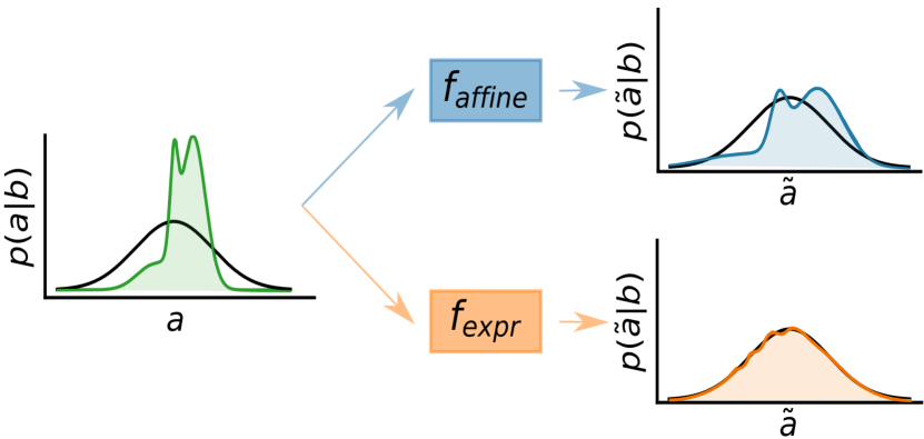
Figure 3: Only coupling functions strictly more expressive than affine can fit non-Gaussian conditionals $p(a_{i}|b)$ in a single block, resulting in a faster loss decrease (Equation 27). Note that coupling flows of both kinds are universal.

Thus, the universality of more expressive coupling functions follows immediately from Theorem 4.6, just like Ishikawa et al. (2022) extended their results from affine to more expressive couplings:

Corollary 4.7.

Coupling-based normalizing flows with coupling functions at least as expressive as affine couplings are distributional universal approximator under the convergence metric $\Delta_{\textnormal{affine}}$ as given in Section 4.4.

Our proof of Theorem 4.6, constructed through layer-wise training, shows how more expressive coupling functions can outperform affine functions using the same number of blocks. Similar to the loss improvement for an affine coupling in Equation 18, let us compute the maximally possible loss improvement for an arbitrarily flexible coupling function:

$$\Delta_{\textnormal{universal}}^{*}=\max_{Q}\mathbb{E}_{b}[J(b)+\Delta_{\textnormal{affine}}^{*}(Q)]\geq\Delta_{\textnormal{affine}}^{*},$$ (27)

where the expectation again goes over the passive coordinate $b=(Qx)_{1,\dots,D/2}$.

Here, the additional loss improvement is the conditional negentropy $J(b)=\sum_{i=1}^{D/2}\mathcal{D}_{\text{KL}}(p_{\theta}(a_{i}|b)\|\mathcal{N}(m_{i}(b),\sigma_{i}(b))$, which measures the deviation of each active dimension from a Gaussian distribution with matching mean and variance. An affine coupling function $c(a_{i};\theta)=sa_{i}+t$ doesn’t influence this term, due to its symmetrical effect on both sides of the KL in $J(p)$ (Draxler et al., 2022, Lemma 1). More expressive coupling blocks, however, are able to tap on this loss component if the conditional distributions $p(a_{i}|b)$ are significantly non-Gaussian, see Figure 3 for an example.

The impact of this gain likely varies with the dataset. For instance, in images, the distribution of one color channel of one pixel conditioned on the other color channels in the entire image, often shows a simple unimodal pattern with low negentropy. This a successful scenario in separating passive and active dimensions in images (Kingma & Dhariwal, 2018). We give additional technical details on Equation 27 and the subsequent arguments in Appendix D.

5 Conclusion

Our new universality proofs show an intriguing hierarchy of the universality of different coupling blocks:

1. Volume-preserving normalizing flows, i.e. flows with a constant volume change such as the coupling-based NICE and GIN (Dinh et al., 2015; Sorrenson et al., 2019) are not universal in KL divergence, meaning that there is a fundamental limit in what distributions they can represent.

2. Affine coupling flows such as RealNVP (Dinh et al., 2017) are distributional universal approximators despite their seemingly restrictive architecture.

3. Coupling flows with more expressive coupling functions are also universal approximators, but they converge faster by tapping on an additional loss component in layer-wise training.

Our work theoretically grounds why coupling blocks are the standard choice for practical applications with normalizing flows, combined with their easy implementation and speed in training and inference. We remove spurious constructions present in previous proofs and use a simple principle instead: Construct a flow layer by layer until no more loss improvement can be achieved.

Using volume-preserving flows may have negatively affected existing work. This shortcoming can be (partially) addressed by choosing or learning a more flexible latent distribution.

Impact Statement

This paper presents work whose goal is to advance the field of Machine Learning. There are many potential societal consequences of our work, none which we feel must be specifically highlighted here.

[appendices] [appendices]1

Appendix A Compatible Coupling Functions

The following lists all coupling functions $c(a;\theta)$ (see Equation 6 for its usage) we are aware of. Our universality guarantees Theorems 4.6 and 4.7 hold for all of them:

• Affine coupling flows as RealNVP (Dinh et al., 2017) and GLOW (Kingma & Dhariwal, 2018):

  $$c(x;\theta)=sx+t.$$ (28)

  Here, $\theta=[s;t]\in\mathbb{R}_{+}\times\mathbb{R}$. Note that NICE (Dinh et al., 2015) is explicitly excluded from this list as it is a volume-preserving flow (see Section 4.2).

• Nonlinear squared flow (Ziegler & Rush, 2019):

  $$c(x;\theta)=ax+b+\frac{c}{1+(dx+h)^{2}},$$ (29)

  for $\theta=[a,b,c,d,h]\in\mathbb{R}_{+}\times\mathbb{R}^{4}$. Choose $c=0$ to obtain an affine coupling.

• Flow++ (Ho et al., 2019):

  $$c(x;\theta)=s\sigma^{-1}\mathopen{}\mathclose{{}\left(\sum_{j=1}^{K}\pi_{j}\sigma\mathopen{}\mathclose{{}\left(\frac{x-\mu_{j}}{\sigma_{j}}}\right)}\right)+t.$$ (30)

  Here, $\theta=[s;t;(\pi_{j},\mu_{j},\sigma_{j})_{j=1}^{K}]\in\mathbb{R}_{+}\times\mathbb{R}\times(\mathbb{R}\times\mathbb{R}\times\mathbb{R}_{+})^{K}$ and $\sigma$ is the logistic function. Choose all $\pi_{j}=0$ except for $\pi_{1}=1$, all $\mu_{j}=0$ and all $\sigma_{j}=1$ to obtain an affine coupling.

• SOS polynomial flows (Jaini et al., 2019):

  $$c(x;\theta)=\int_{0}^{x}\sum_{\kappa=1}^{k}\mathopen{}\mathclose{{}\left(\sum_{l=0}^{r}a_{l,\kappa}u^{l}}\right)^{2}du+t.$$ (31)

  Here, $\theta=[t;(a_{l,\kappa})_{l,\kappa}]\in\mathbb{R}\times\mathbb{R}^{rk}$. Choose all $a_{l,\kappa}=0$ except for $a_{1,0}=s$ to obtain an affine coupling.

• Spline flows in all variants: Cubic (Durkan et al., 2019a), piecewise-linear, monotone quadratic (Müller et al., 2019), and rational quadratic (Durkan et al., 2019b) splines. A spline is parameterized by knots $\theta$ with optional derivative information depending on the spline type, and $c$ computes the corresponding spline function. Choose the spline knots as $y_{i}=sx_{i}+t$ for an affine coupling, choose the derivatives as $x_{i}^{\prime}=s$ for an affine coupling.

• Neural autoregressive flow (Huang et al., 2018) use a feed-forward neural network to parameterize $c(x;\theta)$ by a feed-forward neural network. They show that a neural network is guaranteed to be bijective if all activation functions are strictly monotone and all weights positive. One can construct a ReLU network with a single linear region to obtain an affine coupling.

• Unconstrained monotonic neural networks (Wehenkel & Louppe, 2019) also use a feed-forward neural, but restrict it to have positive output. To obtain $c(x;\theta)$, this function is then numerically integrated with a learnable offset for $x=0$. Choose a constant neural network to obtain an affine coupling.

Appendix B Proofs on Volume-preserving Flows

B.1 Proof of Theorem 4.2

In this section we want to present a two-dimensional example, for which no normalizing flow with constant Jacobian determinant can be constructed such that the KL-divergence between the data distribution and the distribution defined by the normalizing flow is zero.

$$p(x,y)=\begin{cases}0.9&\text{if}\;\;\;(x,y)\in\mathopen{}\mathclose{{}\left[-0.5,0.5}\right]\times\mathopen{}\mathclose{{}\left[-0.5,0.5}\right]\\ 0.9-k\cdot\mathopen{}\mathclose{{}\left(\mathopen{}\mathclose{{}\left|x}\right|-0.5}\right)&\text{if}\;\;\;\mathopen{}\mathclose{{}\left|x}\right|\in\mathopen{}\mathclose{{}\left[0.5,\frac{0.9}{k}+0.5}\right]\land\mathopen{}\mathclose{{}\left|y}\right|\in\mathopen{}\mathclose{{}\left[0,\mathopen{}\mathclose{{}\left|x}\right|}\right]\\ 0.9-k\cdot\mathopen{}\mathclose{{}\left(\mathopen{}\mathclose{{}\left|y}\right|-0.5}\right)&\text{if}\;\;\;\mathopen{}\mathclose{{}\left|y}\right|\in\mathopen{}\mathclose{{}\left[0.5,\frac{0.9}{k}+0.5}\right]\land\mathopen{}\mathclose{{}\left|x}\right|\in\mathopen{}\mathclose{{}\left[0,\mathopen{}\mathclose{{}\left|y}\right|}\right]\\ 0&\text{else}\end{cases}$$ (32)

The data distribution $p(x,y)$ which has to be approximated by the model is defined in (32). This data distribution has a constant value of $0.9$ in a box centered around the origin with a side length of one. This region of constant density is skirted by a margin where the density decreases linearly to zero. Outside the decreasing region, the density is zero. The linear decline is governed by the constant $k$ in (32) which has to be chosen such that the density integrates to one. Since our example only requires the region of constant density but not the decaying tails of it, the exact functional form of the decaying regions are not relevant as long as they lead to a properly normalized distribution. Equation 32 only provides a possible definition of such a density.

To approximate this data distribution a normalizing flow as defined in Section 3 is considered. In this example, we focus on normalizing flows with constant Jacobian determinant. To simplify notation we define $J=\mathopen{}\mathclose{{}\left|f_{\theta}^{\prime}(x)}\right|=const.$

$$A =\mathopen{}\mathclose{{}\left\{(x,y)\in\mathbb{R}^{2}:0.9-\epsilon<p_{\theta}(x,y)}\right\}$$ (33)

$$B =\mathopen{}\mathclose{{}\left[-0.5,0.5}\right]\times\mathopen{}\mathclose{{}\left[-0.5,0.5}\right]$$ (34)

$$\bar{A} =B\char 92\relax A$$ (35)

We choose $\epsilon=0.1$ and use this constant to define the set $A$ (see (33)). In addition we define $B$ which is the region of the data space, where the data distribution has a constant value of $0.9$ (see (34)). $\bar{A}$ is the complement of $A$ on B (see (35)).

$$\Delta_{\textnormal{affine}}(p,p_{\theta})=\sup_{A\;\text{measurable}}\mathopen{}\mathclose{{}\left|P(A)-P_{\theta}(A)}\right|$$ (36)

$$\Delta_{\textnormal{affine}}(p,p_{\theta})\leq\sqrt{\frac{1}{2}D_{KL}(p||p_{\theta})}$$ (37)

The aim of this example, is to find lower bounds for the KL-divergence between the data distribution and the distribution defined by the normalizing flow. To find these bounds we use Pinsker’s inequality (37) (Gibbs & Su, 2002) which links the total variation distance (36) to the Kullback-leibler divergence. It is worth mentioning, that constructing one measurable event for which $\mathopen{}\mathclose{{}\left|P(A)-P_{\theta}(A)}\right|>0$ provides a lower bound for the total variation distance and therefore for the KL divergence.

To construct such an event, we consider two distinct cases, which consider different choice for the normalizing flow, charaterised by the value of the absolute Jacobian determinant.

Case 1: $A=\emptyset$

This case arises if the absolute Jacobin determinant is so small, that the distribution defined by the normalizing flow never exceeds the limit defining $A$ or if it is chosen so large, that the volume of $A$ vanishes.

In this case, we find $\bar{A}=B$ and $|\bar{A}|=1$ where $|\bar{A}|$ denotes the volume of the data space occupied by $\bar{A}$. Using the fact that the data distribution has a constant value of $0.9$ in $B$ and that $p_{\theta}<0.9-\epsilon$ in $\bar{A}=B$,

$$\mathopen{}\mathclose{{}\left|P(\bar{A})-P_{\theta}(\bar{A})}\right| =\mathopen{}\mathclose{{}\left|0.9-P_{\theta}(\bar{A})}\right|$$ (38)

$$\geq\mathopen{}\mathclose{{}\left|0.9\cdot 1-(0.9-\epsilon)\cdot 1}\right|$$ (39)

$$=\mathopen{}\mathclose{{}\left|\epsilon}\right|=\epsilon$$ (40)

Using (40) as a lower bound for the total variation distance (40) we can apply (37) to find (43) as a lower bound for the KL divergence.

$$D_{KL}(p||p_{\theta}) \geq 2\cdot\Delta_{\textnormal{affine}}(p,p_{\theta})^{2}$$ (41)

$$\geq 2\cdot\epsilon^{2}$$ (42)

$$=0.02$$ (43)

Case 2: $A\neq\emptyset$

Inserting the definition of $p_{\theta}(x,y)$ as given in (1) into the definition of $A$ (see 33) and rewriting the condition defining the set yields (44).

$$A=\mathopen{}\mathclose{{}\left\{(x,y)\in\mathbb{R}^{2}:\frac{0.9-\epsilon}{J}<p(z=f_{\theta}(x,y))}\right\}\\$$ (44)

This defines a set $C$ in the latent space which is defined in (45).

$$C=\mathopen{}\mathclose{{}\left\{z\in\mathbb{R}^{2}:\frac{0.9-\epsilon}{J}<p(z)}\right\}$$ (45)

Since the normalizing flows considered in this example have a constant Jacobian, the volume of $A$ in the data space is directly linked to the volume of $C$ in the latent space via (46).

$$|A|=\frac{1}{J}\cdot|C|$$ (46)

The definition of $C$ (45) shows, that $C$ is a circle around the origin of the latent space. To determine the volume of $C$ we compute the radius of this circle. This is done by inserting the definition of the latent distribution, which is a two dimensional standard normal distribution into the condition defining $C$ (see (45)). This yields (47). Since the latent distribution is rotational invariant one can simply look at it as a function of the distance $r$ from the origin. Solving the for $r$ leads to (48).

$$\frac{0.9-\epsilon}{J}<\frac{1}{2\pi}\cdot\exp\mathopen{}\mathclose{{}\left(-\frac{r^{2}}{2}}\right)$$ (47)

$$\Rightarrow r=\sqrt{-2\cdot\log\mathopen{}\mathclose{{}\left(\frac{2\pi\cdot(0.9-\epsilon)}{J}}\right)}$$ (48)

Inserting (48) into the formula for the area of a circle and using (46), yields (50) as an expression for the volume of $A$. The lower bound for the volume of $A$ arises from finding the local maximum (which is also the global maximum) of (50) with respect to the absolute Jacobian determinant $J$.

$$|A| =\frac{1}{J}\cdot\pi\cdot r^{2}$$ (49)

$$=\frac{1}{J}\cdot 2\pi\cdot\log\mathopen{}\mathclose{{}\left(\frac{J}{2\pi\cdot(0.9-\epsilon)}}\right)$$ (50)

$$\leq\frac{1}{e\cdot(0.9-\epsilon)}$$ (51)

As in the previous case, we now compute $\mathopen{}\mathclose{{}\left|P(\bar{A})-P_{\theta}(\bar{A})}\right|$.

$$\mathopen{}\mathclose{{}\left|P(\bar{A})-P_{\theta}(\bar{A})}\right| =\mathopen{}\mathclose{{}\left||\bar{A}|\cdot 0.9-P_{\theta}(\bar{A})}\right|$$ (53)

$$\geq\mathopen{}\mathclose{{}\left||\bar{A}|\cdot 0.9-|\bar{A}|\cdot(0.9-\epsilon)}\right|$$ (54)

$$=|\bar{A}|\cdot\epsilon$$ (55)

$$\geq\mathopen{}\mathclose{{}\left(1-|A|}\right)\cdot\epsilon$$ (56)

$$\geq\mathopen{}\mathclose{{}\left(1-\frac{1}{e\cdot(0.9-\epsilon)}}\right)\cdot\epsilon$$ (57)

Using (41) and (57) as a lower bound for the total variation distance and inserting our choice for $\epsilon$ yields (58) as a lower bound for the KL divergence between the data distribution and the distribution defined by the normalizing flow.

$$D_{KL}(p||p_{\theta}) \geq 2\cdot\mathopen{}\mathclose{{}\left(\epsilon\cdot\mathopen{}\mathclose{{}\left(1-\frac{1}{e\cdot(0.9-\epsilon)}}\right)}\right)^{2}$$ (58)

$$\approx 0.0058$$ (59)

We can conclude, that we have derived lower bounds for the KL divergence between the data distribution and the distribution defined by the normalizing flow, which can not be undercut by any normalizing flow with a constant absolute Jacobian determinant. Therefore, we have proven that the class of normalizing flows with constant (absolute) Jacobian determinant can not approximate arbitrary continuous distributions if one uses the KL divergence as a convergence measure.

B.2 Proof of Corollary 4.3

Definition B.1.

Given a probability density $p(x)$ and a connected set $M\subset\mathbb{R}^{D}$. Then, $M$ is called a mode of $p(x)$ if

$$p(x)=p(y)\quad\forall x,y\in M,$$ (60)

and there is a neighborhood $U$ of $M$ such that:

$$p(x)>p(y)\quad\forall x\in M,y\in U\setminus M.$$ (61)

With this definition of a mode, let us characterize the correspondence between modes of $p_{\theta}(x)$ and $p(z)$ for an volume-preserving flow:

Lemma B.2.

Given a latent probability density $p(z)$, a diffeomorphism $f_{\theta}:\mathbb{R}^{D}\to\mathbb{R}^{D}$ with constant Jacobian determinant $|f_{\theta}^{\prime}(x)|=\operatorname{const}$ and a mode $M\subset\mathbb{R}^{D}$. Then, $f(M)$ is a mode of $p_{\theta}(x)$.

Proof.

We show that $f(M)$ fulfils Definition B.1. First, for every $x,y\in f(M)$: The pre-images of $x,y$ are unique in $M$ as $f$ is bijective, that is: $f^{-1}(x),f^{-1}(y)\in M$. As $M$ is a mode:

$$p(f^{-1}(x))=p(f^{-1}(y)).$$ (62)

We follow:

$$(f_{\sharp}p)(x)=p(f^{-1}(x))|J|=p(f^{-1}(y))|J|=(f_{\sharp}p)(y),$$ (63)

where we have used the change-of-variables formula for bijections and that $|J|=\operatorname{const}$.

Let $U$ be a neighborhood of $M$ such that Equation 61 is fulfilled. As $f$ is continuous, there is a neighborhood $V$ of $f(M)$ such that $V\subseteq f(U)$. Consider $x\in f(M),y\in V\setminus f(M)$. As $M$ is a mode:

$$p(f^{-1}(x))>p(f^{-1}(y)).$$ (64)

Multiplying both sides by $|J|$, we find:

$$(f_{\sharp}p)(x)=p(f^{-1}(x))|J|>p(f^{-1}(y))|J|=(f_{\sharp}p)(y).$$ (65)

Thus, $f(M)$ is a mode of $(f_{\sharp}p)(x)$ by Definition B.1. ∎

This makes us ready for the proof of a generalization of Corollary 4.3:

Theorem B.3.

$p(z)$ and $p_{\theta}(x)$ have the same number of modes.

Proof.

By Lemma B.2, every mode of $p(x)$ implies a mode of $(f_{\sharp}p)(x)$. Also, every mode of $(f_{\sharp}p)(x)$ implies a mode of $(f_{\sharp}^{-1}f_{\sharp}p)(x)=p(x)$. Therefore, there is a one-to-one correspondence of modes between $p(x)$ and $(f_{\sharp}p)(x)$. ∎

Appendix C Proofs on Affine Coupling Flows

C.1 Proof of Theorem 4.4

C.1.1 Underlying theorems

Here, we restate the results from the literature that our main proof is based on:

First, (Eaton, 1986) show that if for some vector-valued random variable $X$ and every pair of orthogonal projections the mean of one projection conditioned on the other is zero, then $X$ follows a spherical distribution:

Theorem C.1 (Eaton (1986)).

Suppose the random vector $X\in\mathbb{R}^{D}$ has a finite mean vector. Assume that for each vector $v\neq 0$ and for each vector $u$ perpendicular to $v$ (i.e. $u\cdot v=0$):

$$\mathbb{E}[u\cdot X|v\cdot X]=0.$$ (66)

Then $X$ is spherical and conversely.

Secondly, Cambanis et al. (1981, Corollary 8a) identifies the Gaussian from all elliptically contoured (which includes spherical) distributions. We write it in the form of Bryc (1995, Theorem 4.1.4):

Theorem C.2 (Bryc (1995)).

Let $p(x)$ be radially symmetric with $\mathbb{E}[\mathopen{}\mathclose{{}\left\|x}\right\|^{\alpha}]<\infty$ for some $\alpha>0$. If

$$\mathbb{E}[\mathopen{}\mathclose{{}\left\|x_{1,\dots,m}}\right\|^{\alpha}|x_{m+1,\dots,n}]=\operatorname{const},$$ (67)

for some $1\leq m<n$, then $p(x)$ is Gaussian.

Finally, Draxler et al. (2020, Theorem 1) show that the explicit form of the maximally achievable loss improvement by an affine coupling block $\Delta_{\textnormal{affine}}^{*}$ if the data is rotated by a fixed rotation layer $Q$ is given by:

$$\Delta_{\textnormal{affine}}^{*}(Q) =\min_{s,t}\mathcal{D}_{\text{KL}}(p_{s,t|Q}(z)\|p(z))$$ (68)

$$=\tfrac{1}{2}\mathbb{E}_{b}\mathopen{}\mathclose{{}\left[m_{i}(b)^{2}+\sigma_{i}(b)^{2}-1-\log\sigma_{i}(b)^{2}}\right].$$ (69)

Here, $s,t$ are the scaling and translation in an affine coupling block (see Equation 28), and we optimize over continuous functions for now. By $p_{s,t|Q}(z)$ we denote the latent distribution achieved if $\tilde{a}(a;b)=s(b)\odot a+t(b)$ is applied to $p(a,b)$, the rotated version of the incoming $p(z)$. The symbols $m_{i}(b),\sigma_{i}(b)^{2}$ are conditional moments of the active dimensions $a_{i}$ conditioned on the passive dimensions $b$:

$$m_{i}(b)=\mathbb{E}_{a_{i}|b}[a_{i}],\qquad\sigma_{i}(b)=\mathbb{E}_{a_{i}|b}[a_{i}^{2}]-m_{i}(b)^{2}.$$ (70)

These conditional moments are continuous functions of $b$ if $p(x)$ is a continuous distribution and $p(b)>0$ for all passive $b\in\mathbb{R}^{D/2}$. The improvement in Equation 69 is achieved by the affine coupling block with the following subnetwork:

$$s_{i}^{*}(b)=\frac{1}{\sigma_{i}(b)},\qquad t_{i}^{*}(b)=-\frac{m_{i}(b)}{\sigma_{i}(b)}.$$ (71)

Note that $s^{*}(b)$ and $t^{*}(b)$ are continuous functions and not actual neural networks. In the next section, we show that a similar statement on practically realizable neural networks that is sufficient for our universality.

C.1.2 Relation to practical neural networks

To relate Equations 71 and 69 to actually realizable networks, which cannot exactly follow the arbitrary continuous functions $s_{i}^{*}(b),t_{i}^{*}(b)$, we show Lemma 4.5 asserting that the fix point of adding coupling layers with continuous functions is the same as that of single-layer neural networks, derived using a universal approximation theorem for neural networks (Hornik, 1991):

Proof.

First, note that $\Delta_{\textnormal{affine}}*(Q)\geq\Delta_{\textnormal{affine}}(Q)\geq 0$ since no practically realizable coupling block can achieve better than Equation 69. Thus, if $\Delta_{\textnormal{affine}}^{*}(Q)=0$, so is $\Delta_{\textnormal{affine}}(Q)=0$.

For the reverse direction, we fix $Q=I$, and otherwise consider a rotated version of $p$. Also, without loss of generalization, we consider one single active dimension $a_{i}$ in the following, but the construction can then be repeated for each other active dimension.

If we apply any affine coupling layer $f_{\text{cpl},\varphi}(a;b)=s_{\varphi}(b)a+t_{\varphi}(b)$, the loss change by this layer can be computed from the theoretical maximal improvement $\Delta_{\textnormal{affine}}^{*}(Q)$ before and after adding this layer $\tilde{\Delta}_{\textnormal{affine}}^{*}(I)$:

$$\Delta_{\textnormal{affine}}(I)=\Delta_{\textnormal{affine}}^{*}(I)-\tilde{\Delta}_{\textnormal{affine}}^{*}(I)=\tfrac{1}{2}\mathbb{E}_{b}\mathopen{}\mathclose{{}\left[m_{i}(b)^{2}+\sigma_{i}(b)^{2}-1-\log\sigma_{i}(b)^{2}}\right]-\tfrac{1}{2}\mathbb{E}_{b}\mathopen{}\mathclose{{}\left[\tilde{m}_{i}(b)^{2}+\tilde{\sigma}_{i}(b)^{2}-1-\log\tilde{\sigma}_{i}(b)^{2}}\right].$$ (72)

The moments after the affine coupling layers read:

$$\tilde{m}_{i}(b)=s_{\varphi}(b)m_{i}(b)+t_{\varphi}(b),\qquad\tilde{\sigma}_{i}(b)=s_{\varphi}(b)\sigma_{i}(b).$$ (73)

Case 1: $\mathbb{E}_{b}[\sigma_{i}(b)^{2}-1-\log\sigma_{i}(b)^{2}]>0$:

Then, without loss of generality, by continuity and positivity of $p$ and consequential continuity of $\sigma_{i}(b)$ in $b$, there is a convex open set $A\subset\mathbb{R}^{D/2}$ with non-zero measure $p(A)>0$ where $\sigma_{i}(b)>1$. If $\sigma_{i}(b)<1$ everywhere, apply the following argument flipped around $\sigma_{i}(b)=1$.

Denote by $\sigma_{\max}=\max_{b\in A}\sigma_{i}(b)$. Then, by continuity of $\sigma_{i}(b)$ there exists $B\subset A$ so that $\sigma_{i}(b)>(\sigma_{\max}-1)/2+1=:\sigma_{\max/2}$ for all $b\in B$. Let $C\subset B$ be a multi-dimensional interval $[l_{1},r_{1}]\times\dots\times[l_{D/2},r_{D/2}]$ with $p(C)>0$ inside of $B$.

Now, we construct a ReLU neural network with two hidden layers with the following property, where $F\subset E\subset C$ are specified later with $p(F)>p(E)>0$:

$$\begin{cases}f_{\varphi}(x)=\frac{1}{\sigma_{\max/2}}&x\in E\subset D\\ \frac{1}{\sigma_{\max/2}}\leq f_{\varphi}(x)<1&x\in D\\ f_{\varphi}(x)=0&\text{else.}\end{cases}$$ (74)

To do so, we make four neurons for each dimension $i=1,\dots,D/2$:

$$\operatorname{ReLU}(x_{i}-l_{i}),\operatorname{ReLU}(x_{i}-l_{i}-\Delta_{\textnormal{affine}}),\operatorname{ReLU}(x_{i}-r_{i}),\operatorname{ReLU}(x_{i}-r_{i}+\delta),$$ (75)

where $0<\Delta_{\textnormal{affine}}<\min_{i}(r_{i}-l_{i})/4$. If we add these four neurons with weights $1,-1,-1,1$, we find the following piecewise function:

$$\begin{cases}0&x\leq l_{i}\\ x-l_{i}&l_{i}<x<l_{i}+\delta\\ \delta&l_{i}+\delta\leq x\leq r_{i}-\delta\\ r_{i}-x&r_{i}-\delta<x<r_{i}\\ 0&r_{i}\leq x.\end{cases}$$ (76)

If we repeat this for each dimension and add together all neurons with the corresponding weights into a single neuron in the second layer, then only inside $D=(l_{1}+\Delta_{\textnormal{affine}},r_{1}-\Delta_{\textnormal{affine}})\times\dots\times(l_{D/2}+\Delta_{\textnormal{affine}},r_{D/2}-\Delta_{\textnormal{affine}})\subset C$ the weighted sum would equal $\delta D/2$. By choosing $\Delta_{\textnormal{affine}}$ as above, this region has nonzero volume. We thus equip the single neuron in second layer with a bias of $-\delta D/2+\epsilon$ for some $\epsilon<\delta$, so that it is constant with value $\epsilon$ inside $E=(l_{1}+\delta-\epsilon,r_{1}-\delta+\epsilon)\times\dots\times(l_{D/2}+\delta+\epsilon,r_{D/2}-\delta-\epsilon)\subset D$ and smoothly interpolates to zero in the rest of $D$.

For the output neuron of our network, we choose weight $(\sigma_{\max/2}-1)/\epsilon$ and bias $1$. By inserting the above construction, we find the network specified in Equation 74.

Now, for all $b\in D$,

$$1<\tilde{\sigma}_{i}(b)<\sigma_{i}(b),$$ (77)

so that

$$\tilde{m}_{i}(b)^{2}+\tilde{\sigma}_{i}(b)^{2}-1-\log\tilde{\sigma}_{i}(b)^{2}<m_{i}(b)^{2}+\sigma_{i}(b)^{2}-1-\log\sigma_{i}(b)^{2}.$$ (78)

Thus, parameters $\varphi$ exist that improve on the loss. (Note that this construction can be made more effective in practice by identifying the sets where $\sigma>1$ resp. $\sigma<1$ and then building neural networks that output one or scale towards $\tilde{\sigma}(b)=1$ everywhere. Because we are only interested in identifying improvement, the above construction is sufficient.)

Now, regrading $t_{\varphi}$, we focus on $\mathbb{E}_{b}[m_{i}(b)^{2}]>0$ (otherwise choose $t_{\varphi}=0$ as a constant, which corresponds to a ReLU network with all weights and biases set to zero):

$$\mathbb{E}_{b}[m_{i}(b)^{2}]>\mathbb{E}_{b}[(s_{\varphi}(b)m_{i}(b)+t_{\varphi}(b))^{2}].$$ (79)

By (Hornik, 1991, Theorem 1) there always is a $t_{\varphi}$ that fulfills this relation.

Case 2: $\mathbb{E}_{b}[\sigma_{i}(b)^{2}-1-\log\sigma_{i}(b)^{2}]=0$. Then, choose the neural network $s_{\varphi}(b)=1$ as a constant. As $\Delta_{\textnormal{affine}}>0$, $\mathbb{E}_{b\sim p(a,b)}[m_{i}(b)^{2}]>0$ and we can use the same argument for the existence of $t_{\varphi}$ as before. ∎

C.1.3 Main proof

We now turn to the proof of Theorem 4.4:

Proof.

The forward direction is trivial: $p(z)=\mathcal{N}(0,I)$ and therefore $\mathcal{D}_{\text{KL}}(p(z)\|\mathcal{N}(0,I))=0$. As adding a identity layer is a viable solution to Equation 17, there is a $\varphi$ with $\mathcal{D}_{\text{KL}}(p_{\varphi}(z)\|\mathcal{N}(0,I))=0$, and thus $\Delta_{\textnormal{affine}}=0$.

For the reverse direction, start with $\Delta_{\textnormal{affine}}=0$. Then, by Lemma 4.5, also $\Delta_{\textnormal{affine}}^{*}=0$.

The maximally achievable loss improvement for any rotation $Q$ is then given by:

$$\Delta_{\textnormal{affine}}^{*}=\max_{Q}\tfrac{1}{2}\mathbb{E}_{b}\mathopen{}\mathclose{{}\left[m_{i}(b)^{2}+\sigma_{i}(b)^{2}-1-\log\sigma_{i}(b)^{2}}\right]=0.$$ (80)

It holds that both $x^{2}\geq 0$ and $x^{2}-1-\log x^{2}\geq 0$. Thus, the following two summands are zero:

$$0 =\tfrac{1}{2}\mathbb{E}_{b}\mathopen{}\mathclose{{}\left[m_{i}(b)^{2}}\right],$$ (81)

$$0 =\tfrac{1}{2}\mathbb{E}_{b}\mathopen{}\mathclose{{}\left[\sigma_{i}(b)^{2}-1-\log\sigma_{i}(b)^{2}}\right].$$ (82)

This holds for all $Q$ since the maximum over $Q$ is zero.

By continuity of $p(b)$ and $m_{1}(b)$ in $p$, this implies for all $b$:

$$\mathbb{E}_{a_{1}|b}[a_{1}]=0.$$ (83)

Fix $b_{1}$ and marginalize out the remaining dimensions $b_{2,\dots D/2}$ to compute the mean of $a_{1}$ conditioned on $b_{1}$:

$$m_{a_{1}|b}=\mathbb{E}_{a_{1}|b_{1}}[a_{1}]=\mathbb{E}_{b_{1,\dots,D/2}}[\mathbb{E}_{a_{1}|b}[a_{1}]]=\mathbb{E}_{b_{1,\dots,D/2}}[0]=0.$$ (84)

As $a_{1}$ and $b_{1}$ are arbitrary orthogonal directions since the above is valid for any $Q$, we can employ Theorem C.1 to follow that $p(x)$ is spherically symmetric.

We are left with showing that for a spherical $p(x)$, if for all $Q$ there is no improvement $\Delta_{\textnormal{affine}}(Q)$, then $p(x)=\mathcal{N}(0,I)$.

Without loss of generality, we can fix $Q=I$, as $(Q_{\sharp}p)(x)=p(x)$ for all $Q$. We write $x=(p;a)$.

As $\Delta_{\textnormal{affine}}=0$, we can follow $\sigma_{i}(b)=1$ like above. This implies that:

$$\mathbb{E}_{a|b}[\mathopen{}\mathclose{{}\left\|a}\right\|^{2}]=\sum_{i=1}^{D/2}(m_{i}(b)^{2}+\sigma_{i}(b)^{2})=D/2.$$ (85)

In particular, this is independent of $b$ and we can thus apply Theorem C.2 with $\alpha=2$.

Finally, $m(b)=0$ and $\sigma_{i}(b)=1$ for all $Q$ imply that $p(x)=\mathcal{N}(0,I)$. ∎

C.2 Proof of Theorem 4.6

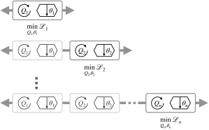
Figure 4: The normalizing flow we construct in our proof is remarkably simple: We iteratively add coupling blocks, optimizing the parameters of the new block while keeping previous parameters fixed. Theorem 4.4 shows that if adding another blocks shows no improvement in the loss, the flow has converged to a standard normal distribution in the latent space. Since the total loss that can be removed is finite, the flow converges.

The proof idea of iteratively adding new layers which are trained without changing previous layers is visualized in Figure 4.

Proof.

Let us consider a coupling-based normalizing flow of depth $n$ and call the corresponding latent distributions $p_{n}(z)$, where $n=0$ corresponds to the initial data distribution $p(x)$. Denote by $\mathcal{L}_{n}=\mathcal{D}_{\text{KL}}(p_{n}(z)\|p(z))$ the corresponding loss. Then, if we add another layer to the flow, we achieve a difference in loss of $\Delta_{{\textnormal{affine}},n}=\mathcal{L}_{n+1}-\mathcal{L}_{n}$.

Without loss of generality, we assume that the rotation layer $Q$ of this additional block can be chosen freely. Otherwise add 48 coupling blocks with fixed rotations that together exactly represent the $Q$ we want, as shown by Koehler et al. (2021, Theorem 2).

We then choose the rotation $Q$ and subnetwork parameters $\varphi$ of the additional block such that it maximally reduces the loss in the sense of Equation 17, keeping the parameters of the previous layers fixed. Then, $\Delta_{{\textnormal{affine}},n}$ attains the value given in Equation 18.

Each layer contributes a non-negative improvement in the loss, which in total can only sum up to the initial loss. For a non-negative series whose total sum is finite, the series must go to zero, which shows convergence in terms of Section 4.4:

$$\sum_{n=0}^{\infty}\Delta_{{\textnormal{affine}},n}\leq\mathcal{L}_{0}<\infty\Rightarrow\Delta_{{\textnormal{affine}},n}\to 0.$$ (86)

∎

C.3 Relation to Convergence in KL

Corollary C.3.

Given a series of probability distributions $p_{n}(z)$. Then, convergence in KL divergence

$$\mathcal{D}_{\text{KL}}(p_{n}(z)\|\mathcal{N}(0,1))\xrightarrow{n\to\infty}0$$ (87)

implies convergence in the convergence metric in Section 4.4:

$$\Delta_{{\textnormal{affine}},n}\xrightarrow{n\to\infty}0.$$ (88)

Proof.

By assumption, for every $\epsilon>0$ there exists $N\in\mathbb{N}$ such that:

$$\mathcal{D}_{\text{KL}}(p_{n}(z)\|\mathcal{N}(0,1))<\epsilon\quad\forall n>N.$$ (89)

This implies convergence of $\Delta_{{\textnormal{affine}},n}$, by the following upper bound via the sum of all possible future improvements which is bounded from above by the total loss:

$$\Delta_{{\textnormal{affine}},n}\leq\sum_{m=n}^{\infty}\Delta_{{\textnormal{affine}},m}\leq\mathcal{D}_{\text{KL}}(p_{n}(z)\|\mathcal{N}(0,1))<\epsilon\quad\forall n>N.$$ (90)

∎

Appendix D Benefits of More Expressive Coupling Blocks

To see what the best improvement for an infinite capacity coupling function can ever be, we make use of the following Pythagorean identity combined from variants in Draxler et al. (2022); Cardoso (2003); Chen & Gopinath (2000):

$$\mathcal{L}=\mathcal{D}_{\text{KL}}(p_{\theta}(z)\|\mathcal{N}(0,I))=P+\mathbb{E}_{b\sim p(a,b)}\mathopen{}\mathclose{{}\left[D(b)+J(b)+S(b)}\right].$$ (91)

The symbols $P,D(b),J(b),S(b)$ all denote KL divergences:

The first two terms remain unchanged under a coupling layer: The KL divergence to the standard normal in the passive dimensions $P=\mathcal{D}_{\text{KL}}(p_{\theta}(b)\|\mathcal{N}(0,I_{D/2}))$, which are left unchanged. The dependence between active dimensions $D(b)=\mathcal{D}_{\text{KL}}(p_{\theta}(a|b)\|p_{\theta}(a_{1}|b)\cdots p_{\theta}(a_{D/2}|b))$ measures the multivariate mutual information between active dimensions. It is unchanged because each dimension $a_{i}$ is treated conditionally independent of the others (Chen & Gopinath, 2000).

The remaining terms measure how far each dimension $p_{\theta}(a_{i}|b)$ differs from the standard normal: The negentropy measures the divergence to the Gaussian with the same first moments as $p_{\theta}(a_{i}|b)$ in each dimension, summing to $J(b)=\sum_{i=1}^{D/2}\mathcal{D}_{\text{KL}}(p_{\theta}(a_{i}|b)\|\mathcal{N}(m_{i}(b),\sigma_{i}(b)))$. Finally, the non-Standardness $S(b)=\sum_{i=1}^{D/2}\mathcal{D}_{\text{KL}}(\mathcal{N}(m_{i}(b),\sigma_{i}(b))\|\mathcal{N}(0,1))$ measures how far these 1d Gaussian are away from the standard normal distribution.

Note that the total loss $\mathcal{L}$ is invariant under a rotation of the data. The rotation does, however, affect how that loss is distributed into the different components in Equation 91.

If we restrict the coupling function to be affine-linear $c(a_{i};\theta)=sa_{i}+t$ (i.e. a RealNVP coupling), then this means that also $J(b)$ is left unchanged, essentially because $p_{\theta}(a_{i}|b)$ and $\mathcal{N}(m_{i}(b),\sigma_{i}(b))$ undergo the same transformation (Draxler et al., 2022, Lemma 1). Only a nonlinear coupling function $c(a_{i};\theta)$ can thus affect $J(b)$ and reduce it to $\tilde{J}(b)<J(b)$ (if $J(b)>0$).

Taking the loss difference between two layers, we find Equation 27.

Appendix E Experimental details

We base our code on PyTorch (Paszke et al., 2019), Numpy (Harris et al., 2020), Matplotlib (Hunter, 2007) for plotting and Pandas (Wes McKinney, 2010; The pandas development team, 2020) for data evaluation.

We provide our code at https://github.com/vislearn/Coupling-Universality. Sequentially running all experiments takes less than two hours on a desktop computer with a GTX 2080 GPU.

E.1 Layer-wise flow

In experiment on a toy dataset for Figure 1, we demonstrate that a coupling flow constructed layer by layer as in Equation 22 learns a target distribution. We proceed as follows:

We construct a data distribution on a circle as a Gaussian mixture of $M$ Gaussians with means $m_{i}=(r\cos\varphi_{i},r\sin\varphi_{i})$, where $\varphi_{i}=0,\frac{1}{M}2\pi,\dots,\frac{M-1}{M}2\pi$ are equally spaced, and $\sigma_{i}=0.3$. The advantage of approximating the ring with this construction is that this yields a simple to evaluate data density, which we need for accurately plotting $p_{\theta}(z)$:

$$p(x)=\frac{1}{M}\sum_{i=1}^{M}\mathcal{N}(x;m_{i},\sigma^{2}I).$$ (92)

We then fit a total 100 layers in the following way: First, treat $p(x)$ as the initial guess for the latent distribution. Then, we build the affine coupling block that maximally reduces the loss using Equation 22. We therefore need to know the conditional mean $m(b)$ and standard deviation $\sigma(b)$ for each $b$. We approximate this from a finite number of samples $N$ which are grouped by the passive coordinate $b$ into $B$ bins so that $N/B$ samples are in each bin. We then compute the empirical mean $m_{i}$ and standard deviation $\sigma_{i}$ over the active dimension in each bin $i=1,\dots,B$. According to Equation 22, we define $s_{i}=\frac{1}{\sigma_{i}}$ and $t_{i}=-\frac{1}{\sigma_{i}}m_{i}$ at the bin centers and interpolate between bins using a cubic spline. Outside of the domain of the splines, we extrapolate constant $s,t$ with the value of the closest bin. We do not directly optimize over $Q$, but choose the $Q$ that reduces the loss most out of $N_{Q}$ random 2d rotation matrices.

We limit the step size of each layer to avoid artifacts from finite training data, by mapping:

$$\tilde{x}=\alpha x+(1-\alpha)f_{\text{blk}}(x).$$ (93)

In addition, we resample the training data from the ground truth distribution after every step to avoid overfitting.

We choose $N=2^{26}$, $B=64$, $M=20$, $\alpha=0.5$, $N_{Q}=10$. The resulting flow has $64\cdot 2\cdot 100=12,800$ learnable parameters.

E.2 Volume-preserving flows

The target distribution is a two-dimensional Gaussian Mixture Model with two modes. The two modes have the same relative weight but different covariance matrices.

The normalizing flow with a constant Jacobian determinant consists of 15 GIN coupling blocks as introduced in Sorrenson et al. (2019). This type of coupling blocks has a Jacobin determinant of one. To allow volume scaling a layer with a learnable global scaling is added after the final coupling block. This learnable weight is initialized as one. For the normalizing flow with variable Jacobin determinant, the GIN coupling is modified by removing the normalization of the scaling factors in the affine couplings. This allows the normalizing flow to have variable Jacobian determinants. In this case, the global scaling block is omitted. To implement the normalizing flows we use the FrEIA package (Ardizzone et al., 2018a) implementation of the GIN coupling blocks.

In both normalizing flows, the two sub-networks used to compute the parameters of the affine couplings are fully connected neural networks with two hidden layers and a hidden dimensionality of 128. ReLU activations are used. The weights of the linear layers of the subnetworks are initialized by applying the PyTorch implementation of the Xavier initialization (Glorot & Bengio, 2010). In addition, the weights and biases of the final layer of each sub-networks are set to zero.

The networks are trained using the Adam (Kingma & Ba, 2017) with PyTorch’s default settings and a initial learning rate of $1\cdot 10^{-3}$ which is reduced by a factor of ten after $5000,10000$ and $15000$ training iterations. In total, the training ran for $25000$ iterations. In each iteration, a batch of size $128$ was drawn from the target distribution to compute the negative log likelihood objective. We use a standard normal distribution as latent distribution.

[appendices]

References

- Ardizzone et al. (2018a) Ardizzone, L., Bungert, T., Draxler, F., Köthe, U., Kruse, J., Schmier, R., and Sorrenson, P. Framework for Easily Invertible Architectures (FrEIA), 2018a.
- Ardizzone et al. (2018b) Ardizzone, L., Kruse, J., Rother, C., and Köthe, U. Analyzing Inverse Problems with Invertible Neural Networks. In International Conference on Learning Representations, 2018b.
- Bryc (1995) Bryc, W. The Normal Distribution, volume 100 of Lecture Notes in Statistics. Springer New York, New York, NY, 1995. ISBN 978-0-387-97990-8 978-1-4612-2560-7. doi: 10.1007/978-1-4612-2560-7.
- Cambanis et al. (1981) Cambanis, S., Huang, S., and Simons, G. On the theory of elliptically contoured distributions. Journal of Multivariate Analysis, 11(3):368–385, September 1981. ISSN 0047259X. doi: 10.1016/0047-259X(81)90082-8.
- Cardoso (2003) Cardoso, J.-F. Dependence, Correlation and Gaussianity in Independent Component Analysis. Journal of Machine Learning Research, 4:1177–1203, 2003. ISSN 1532-4435.
- Chen & Gopinath (2000) Chen, S. and Gopinath, R. Gaussianization. In Leen, T., Dietterich, T., and Tresp, V. (eds.), Advances in Neural Information Processing Systems, volume 13. MIT Press, 2000.
- Dibak et al. (2022) Dibak, M., Klein, L., Krämer, A., and Noé, F. Temperature steerable flows and Boltzmann generators. Phys. Rev. Res., 4(4):L042005, October 2022. doi: 10.1103/PhysRevResearch.4.L042005.
- Dinh et al. (2015) Dinh, L., Krueger, D., and Bengio, Y. NICE: Non-linear Independent Components Estimation. In International Conference on Learning Representations, Workshop Track, 2015.
- Dinh et al. (2017) Dinh, L., Sohl-Dickstein, J., and Bengio, S. Density estimation using Real NVP. In International Conference on Learning Representations, 2017.
- Draxler et al. (2020) Draxler, F., Schwarz, J., Schnörr, C., and Köthe, U. Characterizing the Role of a Single Coupling Layer in Affine Normalizing Flows. In German Conference on Pattern Recognition, 2020.
- Draxler et al. (2022) Draxler, F., Schnörr, C., and Köthe, U. Whitening Convergence Rate of Coupling-based Normalizing Flows. In NeurIPS, 2022.
- Draxler et al. (2023) Draxler, F., Kühmichel, L., Rousselot, A., Müller, J., Schnoerr, C., and Koethe, U. On the convergence rate of gaussianization with random rotations. In International Conference on Machine Learning, 2023.
- Durkan et al. (2019a) Durkan, C., Bekasov, A., Murray, I., and Papamakarios, G. Cubic-Spline Flows. In International Conference on Machine Learning, Workshop Track, 2019a. doi: 10.48550/ARXIV.1906.02145.
- Durkan et al. (2019b) Durkan, C., Bekasov, A., Murray, I., and Papamakarios, G. Neural spline flows. Advances in neural information processing systems, 32, 2019b.
- Eaton (1986) Eaton, M. L. A characterization of spherical distributions. Journal of Multivariate Analysis, 20(2):272–276, December 1986. ISSN 0047259X. doi: 10.1016/0047-259X(86)90083-7.
- Gibbs & Su (2002) Gibbs, A. L. and Su, F. E. On Choosing and Bounding Probability Metrics. International Statistical Review / Revue Internationale de Statistique, 70(3):419–435, 2002. ISSN 03067734, 17515823.
- Glorot & Bengio (2010) Glorot, X. and Bengio, Y. Understanding the difficulty of training deep feedforward neural networks. In Teh, Y. W. and Titterington, M. (eds.), Proceedings of the Thirteenth International Conference on Artificial Intelligence and Statistics, volume 9 of Proceedings of Machine Learning Research, pp. 249–256, Chia Laguna Resort, Sardinia, Italy, 13–15 May 2010. PMLR. URL https://proceedings.mlr.press/v9/glorot10a.html.
- Harris et al. (2020) Harris, C. R., Millman, K. J., van der Walt, S. J., Gommers, R., Virtanen, P., Cournapeau, D., Wieser, E., Taylor, J., Berg, S., Smith, N. J., Kern, R., Picus, M., Hoyer, S., van Kerkwijk, M. H., Brett, M., Haldane, A., del Río, J. F., Wiebe, M., Peterson, P., Gérard-Marchant, P., Sheppard, K., Reddy, T., Weckesser, W., Abbasi, H., Gohlke, C., and Oliphant, T. E. Array programming with NumPy. Nature, 585(7825):357–362, 2020.
- Ho et al. (2019) Ho, J., Chen, X., Srinivas, A., Duan, Y., and Abbeel, P. Flow++: Improving Flow-Based Generative Models with Variational Dequantization and Architecture Design. In International Conference on Machine Learning, 2019.
- Hoogeboom et al. (2022) Hoogeboom, E., Satorras, V. G., Vignac, C., and Welling, M. Equivariant diffusion for molecule generation in 3d. In International Conference on Machine Learning, pp. 8867–8887. PMLR, 2022.
- Hornik (1991) Hornik, K. Approximation capabilities of multilayer feedforward networks. Neural Networks, 4(2):251–257, 1991. ISSN 08936080. doi: 10.1016/0893-6080(91)90009-T.
- Huang et al. (2018) Huang, C.-W., Krueger, D., Lacoste, A., and Courville, A. Neural Autoregressive Flows. In International Conference on Machine Learning, 2018.
- Huang et al. (2020) Huang, C.-W., Dinh, L., and Courville, A. Augmented Normalizing Flows: Bridging the Gap Between Generative Flows and Latent Variable Models. In International Conference on Learning Representations, Workshop Track, 2020.
- Hunter (2007) Hunter, J. D. Matplotlib: A 2D graphics environment. Computing in Science & Engineering, 9(3):90–95, 2007.
- Ishikawa et al. (2022) Ishikawa, I., Teshima, T., Tojo, K., Oono, K., Ikeda, M., and Sugiyama, M. Universal approximation property of invertible neural networks. arXiv preprint arXiv:2204.07415, 2022.
- Jaini et al. (2019) Jaini, P., Selby, K. A., and Yu, Y. Sum-of-Squares Polynomial Flow. In International Conference on Machine Learning, 2019.
- Kingma & Ba (2017) Kingma, D. P. and Ba, J. Adam: A method for stochastic optimization, 2017.
- Kingma & Dhariwal (2018) Kingma, D. P. and Dhariwal, P. Glow: Generative flow with invertible 1x1 convolutions. In Advances in Neural Information Processing Systems, 2018.
- Kobyzev et al. (2021) Kobyzev, I., Prince, S. J., and Brubaker, M. A. Normalizing Flows: An Introduction and Review of Current Methods. IEEE Transactions on Pattern Analysis and Machine Intelligence, 43(11):3964–3979, 2021. ISSN 0162-8828, 2160-9292, 1939-3539. doi: 10.1109/TPAMI.2020.2992934.
- Koehler et al. (2021) Koehler, F., Mehta, V., and Risteski, A. Representational aspects of depth and conditioning in normalizing flows. In International Conference on Machine Learning, 2021.
- Köthe (2023) Köthe, U. A review of change of variable formulas for generative modeling. arXiv preprint arXiv:2308.02652, 2023.
- Lee et al. (2021) Lee, H., Pabbaraju, C., Sevekari, A. P., and Risteski, A. Universal approximation using well-conditioned normalizing flows. In Ranzato, M., Beygelzimer, A., Dauphin, Y., Liang, P., and Vaughan, J. W. (eds.), Advances in Neural Information Processing Systems, volume 34, pp. 12700–12711. Curran Associates, Inc., 2021.
- Lyu et al. (2022) Lyu, J., Chen, Z., Feng, C., Cun, W., Zhu, S., Geng, Y., Xu, Z., and Chen, Y. Universality of parametric Coupling Flows over parametric diffeomorphisms. arXiv preprint arXiv:2202.02906, 2022.
- Müller et al. (2019) Müller, T., Mcwilliams, B., Rousselle, F., Gross, M., and Novák, J. Neural Importance Sampling. ACM Transactions on Graphics, 38(5):1–19, 2019. ISSN 0730-0301. doi: 10.1145/3341156.
- Paszke et al. (2019) Paszke, A., Gross, S., Massa, F., Lerer, A., Bradbury, J., Chanan, G., Killeen, T., Lin, Z., Gimelshein, N., Antiga, L., et al. Pytorch: An imperative style, high-performance deep learning library. Advances in neural information processing systems, 32, 2019.
- Rezende & Mohamed (2015) Rezende, D. and Mohamed, S. Variational inference with normalizing flows. In Bach, F. and Blei, D. (eds.), ICML, July 2015.
- Rombach et al. (2022) Rombach, R., Blattmann, A., Lorenz, D., Esser, P., and Ommer, B. High-resolution image synthesis with latent diffusion models. In Proceedings of the IEEE/CVF Conference on Computer Vision and Pattern Recognition, pp. 10684–10695, 2022.
- Sorrenson et al. (2019) Sorrenson, P., Rother, C., and Köthe, U. Disentanglement by nonlinear ICA with general incompressible-flow networks (GIN). In International Conference on Learning Representations, 2019.
- Teshima et al. (2020a) Teshima, T., Ishikawa, I., Tojo, K., Oono, K., Ikeda, M., and Sugiyama, M. Coupling-based Invertible Neural Networks Are Universal Diffeomorphism Approximators. In Advances in Neural Information Processing Systems, 2020a.
- Teshima et al. (2020b) Teshima, T., Tojo, K., Ikeda, M., Ishikawa, I., and Oono, K. Universal Approximation Property of Neural Ordinary Differential Equations. In Advances in Neural Information Processing Systems, Workshop Track, 2020b.
- The pandas development team (2020) The pandas development team. Pandas-dev/pandas: Pandas, February 2020.
- Wehenkel & Louppe (2019) Wehenkel, A. and Louppe, G. Unconstrained Monotonic Neural Networks. In Advances in Neural Information Processing Systems, 2019.
- Wes McKinney (2010) Wes McKinney. Data Structures for Statistical Computing in Python. In van der Walt, S. and Jarrod Millman (eds.), 9th Python in Science Conference, 2010.
- Zhang et al. (2020) Zhang, H., Gao, X., Unterman, J., and Arodz, T. Approximation Capabilities of Neural ODEs and Invertible Residual Networks. In International Conference on Machine Learning, 2020.
- Ziegler & Rush (2019) Ziegler, Z. and Rush, A. Latent Normalizing Flows for Discrete Sequences. In International Conference on Machine Learning, 2019.
[appendices] \printcontents[appendices]1