[#1][Restated]

Bandit Convex Optimisation

Chapter 1  Introduction and problem statement

Bandit problems are most commonly thought of in terms of sequential decision making or as an elementary version of reinforcement learning. This is certainly true, but they are also intimately connected with optimisation. These notes focus on the convex bandit problem, where the set of actions is a convex subset of euclidean space and the function mapping actions to losses is convex. The learner chooses actions and observes the corresponding loss, possibly with additive noise. The duty of the learner is to minimise the loss. When phrased like this the problem seems more like zeroth-order optimisation and these notes largely take that viewpoint. We do borrow two key notions from the bandit community that give the algorithms and analysis a unique flavour:

• We focus on the cumulative regret as a performance criterion; and

• We (mostly) consider the adversarial setting, where the loss function is changing from one query to the next.

These differences mean the algorithms and theorems presented here are often not directly comparable to standard settings in the optimisation literature. Generally speaking, the theorems presented here hold with fewer assumptions and consequentially are sometimes weaker.

1.1  Prerequisites

Most readers will benefit from a reasonable knowledge of online learning (Cesa-Bianchi and Lugosi, 2006; Hazan, 2016; Orabona, 2019) and bandits (Bubeck and Cesa-Bianchi, 2012; Slivkins, 2019; Lattimore and Szepesvári, 2020). We use some theory from interior point methods, which you could refresh by reading the lecture notes by Nemirovski (1996). None of this is essential, however, if you are prepared to take a few results on faith. Similarly, we use a few simple results from concentration of measure. Our reference was the book by Vershynin (2018) but Boucheron et al. (2013) also covers the material needed. We do use martingale versions of these results, which sadly do not appear in these books but are more-or-less trivial extensions. The symbol () on a proof, section or chapter means that you could (should?) skip this part on your first pass.

1.2  Bandit convex optimisation

Let $K\subset\mathbb{R}^{d}$ be convex and $f_{1},\ldots,f_{n}:\mathbb{R}^{d}\to\mathbb{R}\cup\{\infty\}$ be an unknown sequence of convex functions with $K\subset\operatorname{dom}(f_{t})=\{x:f_{t}(x)<\infty\}$. A learner interacts with the environment over $n$ rounds. In round $t$ the learner is told $\operatorname{dom}(f_{t})$ and chooses an action $X_{t}\in\operatorname{dom}(f_{t})$. They then observe a noisy loss $Y_{t}=f_{t}(X_{t})+\varepsilon_{t}$, where $(\varepsilon_{t})_{t=1}^{n}$ is a sequence of noise random variables. The precise conditions on the noise are given in Eq. 1.1 below but for now you could think of the noise as a sequence of independent standard Gaussian random variables. The learner’s decision $X_{t}$ is allowed to depend on an exogenous source of randomness and the data observed already, which is $\operatorname{dom}(f_{1}),X_{1},Y_{1},\ldots,X_{t-1},Y_{t-1},\operatorname{dom}(f_{t})$. In most applications $\operatorname{dom}(f_{t})=K$. Our main performance metric is the regret, which is

$$\textrm{Reg}_{n}=\max_{x\in K}\sum_{t=1}^{n}(f_{t}(X_{t})-f_{t}(x))\,.$$

The regret is a random variable with the randomness coming from both the noise and the learner’s decisions. We will normally bound the regret in expectation or high probability, depending on what is most convenient. Of course the regret also depends on the loss functions. In general we will try to argue that our algorithms have small regret for any convex losses within some class. Stronger assumptions (smaller classes) lead to stronger results and/or simpler and/or more efficient algorithms. The following definition and notation is sufficient for our purposes.

Definition 1.1.

Let $\mathscr{F}$ be the space of convex functions from $\mathbb{R}^{d}$ to $\mathbb{R}\cup\{\infty\}$ with $K\subset\operatorname{dom}(f)$ and define the following properties of a function $f\in\mathscr{F}$:

1. $f$ is bounded: $f(x)\in[0,1]$ for all $x\in\operatorname{dom}(f)$.

2. $f$ is Lipschitz: $f(x)-f(y)\leq\left\|x-y\right\|$ for all $x\in\operatorname{dom}(f)$.

3. $f$ is $\beta$-smooth: $f(x)-\frac{\beta}{2}\left\|x\right\|^{2}$ is concave on $\operatorname{dom}(f)$.

4. $f$ is $\alpha$-strongly convex: $f(x)-\frac{\alpha}{2}\left\|x\right\|^{2}$ is convex on $\operatorname{dom}(f)$.

5. $f$ is linear on $\operatorname{dom}(f)$.

6. $f$ is quadratic on $\operatorname{dom}(f)$.

7. $\operatorname{dom}(f)\supset\bigcup_{x\in K}\left(x+\mathbb{B}^{d}_{\varrho}\right)$ where $x+\mathbb{B}^{d}_{\varrho}=\{y:\left\|x-y\right\|\leq\varrho\}$.

8. There exists a convex function $g:\mathbb{R}^{d}\to\mathbb{R}$ such that $f(x)=g(x)$ on $\operatorname{dom}(f)$ and $g$ is $\beta$-smooth and $\alpha$-strongly convex on $\mathbb{R}^{d}$.

Property (u) means that $f$ is defined on some expansion of $K$ and the learner may query the function outside of $K$ but is nevertheless compared to the best point in $K$. Property (e) is only relevant when $f$ is assumed to be smooth and strongly convex on $\operatorname{dom}(f)$ and asserts the existence of a smooth and strongly convex extension of $f$ to all of $\mathbb{R}^{d}$ but the learner is still only allowed to query $f$ on $\operatorname{dom}(f)$. The existence of such an extension is often technically convenient but surprisingly not always possible (Drori, 2018). Fortunately there are ways to circumvent this problem, which we explain in Chapter 3. We use the property symbols to define subsets of $\mathscr{F}$. For example:

• $\mathscr{F}_{\tiny{\texttt{b}}}=\{f\in\mathscr{F}:f(x)\in[0,1]\text{ for all }x\in K\}$.

• $\mathscr{F}_{\tiny{\texttt{b}},\tiny{\texttt{sm}},\tiny{\texttt{sc}}}$ is the set of bounded convex functions that are smooth and strongly convex.

When smoothness and strong convexity are involved, our bounds will depend on the parameters $\alpha>0$ and $0<\beta<\infty$, which we assume are known constants. Similarly, for the unconstrained setting the bounds will depend on $\varrho$. The name “unconstrained” is a misnomer, since the learner is still restricted to play in $\operatorname{dom}(f)$. The setting may seem very unusual but arises naturally when $\varrho=\infty$ and $K$ is some subset in which the minimiser of the losses is known to lie.

Noise

Our assumption on the noise is that the sequences $(\varepsilon_{t})_{t=1}^{n}$ is conditionally subgaussian. By this we mean that

$$\mathbb{E}\left[\varepsilon_{t}\mid X_{1},Y_{1},\ldots,X_{t-1},Y_{t-1},X_{t}\right] =0\,;\text{ and}$$

$$\mathbb{E}\left[\exp\left(\varepsilon_{t}^{2}\right)\mid X_{1},Y_{1},\ldots,X_{t-1},Y_{t-1},X_{t}\right] \leq 2\,.$$ (1.1)

This definition of subgaussianity is based on the Orlicz norm definitions. We give a brief summary in Appendix B or you can read the wonderful book by Vershynin (2018). Sometimes we work in the noise free setting where $\varepsilon_{t}=0$ almost surely.

1.3  Settings

There are many variants of bandit convex optimisation. We already outlined some of the assumptions on the function class to which the losses belong. The other major classification is whether or not the problem is adversarial or stochastic.

Adversarial bandit convex optimisation

In the adversarial setting the most common assumption is that the noise $\varepsilon_{t}=0$ while the functions $f_{1},\ldots,f_{n}$ are chosen in an arbitrary way by the adversary. Sometimes the adversary is allowed to choose $f_{t}$ at the same time as the learner chooses $X_{t}$, in which case we say the adversary is non-oblivious. Perhaps more commonly, however, the adversary is obliged to choose all loss functions $f_{1},\ldots,f_{n}$ before the interaction starts. Adversaries of this kind are called oblivious. For our purposes it is convenient to allow non-zero noise even in the adversarial case for reasons that will become apparent in Chapter 3. In any case, the presence of noise does not hurt any of the results in these notes except to change a few constants.

Stochastic bandit convex optimisation

The stochastic setting is more classical. The loss function is now constant over time: $f_{t}=f$ for all rounds $t$ and unknown $f$. The standard performance metric in bandit problems is the regret, but in the stochastic setting it also makes sense to consider the simple regret. At the end of the interaction the learner is expected to output one last point $\widehat{X}\in K$ and the simple regret is

$$\textrm{sReg}_{n}=f(\widehat{X})-\min_{x\in K}f(x)\,.$$

Thanks to convexity there is a straightforward reduction from cumulative regret to simple regret. Simply let $\widehat{X}=\frac{1}{n}\sum_{t=1}^{n}X_{t}$. Then by convexity,

$$\textrm{sReg}_{n}\leq\frac{1}{n}\textrm{Reg}_{n}\,.$$ (1.2)

Another standard measure of performance in the stochastic setting is the sample complexity, which is the number of interactions needed before the simple regret is at most $\varepsilon>0$ with high probability. Our focus for the remainder is on the cumulative regret, but we occasionally highlight the sample complexity of algorithms in order to compare to the literature. The arguments above show that bounds on the cumulative regret imply bounds on the simple regret and sample complexity. The converse is not true.

Regret is random

You should note that $\textrm{Reg}_{n}$ and $\textrm{sReg}_{n}$ are random variables with the randomness arising from both the algorithm and the noise. Most of our results either control $\mathbb{E}[\textrm{Reg}_{n}]$ or prove that $\textrm{Reg}_{n}$ is bounded by such-and-such with high probability. Bounds that hold with high probability are generally preferred since they can be integrated to obtain bounds in expectations. But we will not be too dogmatic about this. Indeed, we mostly prove bounds in expectation to avoid tedious concentration of measure calculations. As far as we know, these always work out if you try hard enough.

1.4  Notation

Norms

The norm $\left\|\cdot\right\|$ is the euclidean norm for vectors and the spectral norm for matrices. For positive definite $A$, $\left\langle x,y\right\rangle_{A}=x^{\top}Ay$ and $\left\|x\right\|^{2}_{A}=\left\langle x,x\right\rangle_{A}$. Given a random variable $X$, $\left\|X\right\|_{\psi_{k}}=\inf\{t:\mathbb{E}[\exp(|X|^{k}/t)]\leq 2\}$ for $k\in\{1,2\}$ are the Orlicz norms. Remember, $X$ is subgaussian if $\left\|X\right\|_{\psi_{2}}<\infty$ and subexponential if $\left\|X\right\|_{\psi_{1}}<\infty$. You can read more about the Orlicz norms in Appendix B.

Sets

The ball is $\mathbb{B}^{d}_{r}=\{x\in\mathbb{R}^{d}:\left\|x\right\|\leq r\}$ and sphere embedded in $d$ dimensions is $\mathbb{S}^{d-1}_{r}=\{x\in\mathbb{R}^{d}:\left\|x\right\|=r\}$. Hopefully the latter is not confused with the space of positive definite matrices on $\mathbb{R}^{d}$, which we denote by $\mathbb{S}^{d}_{+}$. Given $x\in\mathbb{R}^{d}$ and positive definite matrix $A$ with eigenvalues $(\lambda_{k})_{k=1}^{d}$, we let $E(x,A)=\{y\in\mathbb{R}^{d}:\left\|x-y\right\|_{A^{-1}}\leq 1\}$, which is an ellipsoid centered at $x$ with principle axes of lengths $(\lambda_{k}^{1/2})_{k=1}^{d}$. The space of probability measures on $K\subset\mathbb{R}^{d}$ is $\Delta_{K}$ where we always take the Borel $\sigma$-algebra. The space of measures on $K$ is $\mathscr{M}(K)$, also with the Borel $\sigma$-algebra, denoted by $\mathscr{B}(K)$. For $x,y\in\mathbb{R}^{d}$ we let $[x,y]=\{(1-\lambda)x+\lambda y:\lambda\in[0,1]\}$.

Basic

Given a set $A\subset\mathbb{R}^{d}$ and $x\in\mathbb{R}^{d}$ we let $x+A=\{x+a:a\in A\}$ be the Minkowski sum of $A$ and $\{x\}$. The boundary of $A$ is $\partial A=\{x\in A:\mathbb{B}^{d}_{\varepsilon}\not\subset A\text{ for all }\varepsilon>0\}$ and the interior is $\operatorname{int}(A)=A\setminus\partial A$. The polar of $A$ is $A^{\circ}=\{u:\sup_{x\in A}\left\langle x,u\right\rangle\leq 1\}$. We use $\mathds{1}$ for the identity matrix and $\bm{0}$ for the zero matrix or zero vector. Dimensions and types will always be self-evident from the context. The euclidean projection onto $K$ is $\Pi_{K}(x)=\operatornamewithlimits{arg\,min}_{y\in K}\left\|x-y\right\|$. The interior of a convex body $K$ is $\operatorname{int}(K)=\{x:x+\mathbb{B}^{d}_{\varepsilon}\subset K\text{ for some }\varepsilon>0\}$. The sign function is

$$\operatorname{sign}(x)=\begin{cases}-1&\text{if }x<0\\ 0&\text{if }x=0\\ 1&\text{if }x>0\,.\end{cases}$$

Suppose that $f:\mathbb{R}^{d}\supset A\to\mathbb{R}$ is differentiable at $x\in A$, then we write $f^{\prime}(x)$ for its gradient and $f^{\prime\prime}(x)$ for its Hessian. When $f$ is convex we write $\partial f(x)$ for the set of subderivatives of $f$ at $x$. More generally, $Df(x)[h]$ is the directional derivative of $f$ at $x$ in the direction $h$. Higher-order directional derivatives are denoted by $D^{k}f(x)[h_{1},\ldots,h_{k}]$. Densities are always with respect to the Lebesgue measure. The diameter and condition number of a set $K$ are

$$\operatorname{diam}(K) =\max_{x,y\in K}\left\|x-y\right\| \operatorname{cond}(K) =\frac{\min\{R:K\subset x+\mathbb{B}^{d}_{R},x\in\mathbb{R}^{d}\}}{\max\{r:x+\mathbb{B}^{d}_{r}\subset K,x\in\mathbb{R}^{d}\}}\,.$$

Given a convex set $K$ and continuous function $f:K\to\mathbb{R}$ for which directional derivatives exist on $\operatorname{int}(K)$, we let

$$\operatorname{lip}_{K}(f)=\sup_{x\in\operatorname{int}(K)}\sup_{\nu\in\mathbb{S}^{d-1}_{1}}Df(x)[\nu]\,.$$

Note that convex functions always have directional derivatives on the interior of their domain.

Probability spaces

We will not formally define the probability space on which the essential random variables $X_{1},Y_{1},\ldots,X_{n},Y_{n}$ live. You can see how this should be done in the book by Lattimore and Szepesvári (2020). In general $\mathbb{P}$ is the probability measure on some space carrying these random variables and we let $\mathscr{F}_{t}=\sigma(X_{1},Y_{1},\ldots,X_{t},Y_{t})$ be the $\sigma$-algebra generated by the first $t$ rounds of interaction. We abbreviate $\mathbb{P}_{t}(\cdot)=\mathbb{P}(\cdot|\mathscr{F}_{t})$ and $\mathbb{E}_{t}[\cdot]=\mathbb{E}[\cdot|\mathscr{F}_{t}]$.

Regret

Recall the regret is

$$\textrm{Reg}_{n}=\sup_{x\in K}\sum_{t=1}^{n}(f_{t}(X_{t})-f_{t}(x))\,.$$

We occasionally need the regret relative to a specific $x\in K$, which is

$$\textrm{Reg}_{n}(x)=\sum_{t=1}^{n}(f_{t}(X_{t})-f_{t}(x))\,.$$

Chapter 2  Overview of methods and history

2.1  Methods for bandit convex optimisation

Methods for bandit convex optimisation can be characterised into five classes:

• Cutting plane methods are important theoretical tools for linear programming and non-smooth convex optimisation. The high-level idea is to iteratively cut away pieces of $K$ that have large volume while ensuring that the minimiser stays inside the active set. At least two works have adapted these ideas to stochastic convex bandits, both based on the ellipsoid method (Agarwal et al., 2011; Lattimore and György, 2021a). Cutting plane methods are the geometric version of elimination algorithms for bandits and consequentially are typically analysed in the stochastic setting. We discuss a simple bisection algorithm in Chapter 4 for one-dimensional convex bandits and the ellipsoid method in Chapter 10 for the general case.

• Gradient descent is the fundamental algorithm for (convex) optimisation and a large proportion of algorithms for convex bandits use it as a building block (Kleinberg, 2005; Flaxman et al., 2005; Saha and Tewari, 2011; Hazan and Levy, 2014, and more). At a high level the idea is to estimate gradients of a smoothed version of the loss and use these in gradient descent in place of the real unknown gradients. We explore this idea in depth in Chapters 5 and 6.

• Newton’s method is a second-order method that uses curvature information as well as the gradient. One of the challenges in bandit convex optimisation is that algorithms achieving optimal regret need to behave in a way that depends on the curvature. Second-order methods that estimate the Hessian of the actual loss or a surrogate have been used for bandit convex optimisation by (Suggala et al., 2021; Lattimore and György, 2023) and are the topic of Chapter 9.

• Continuous exponential weights is a powerful algorithm for full information online learning and has been used for convex bandits by Bubeck et al. (2017), who combined it with the surrogate loss function described in Chapter 11 along with many tricks to construct the first polynomial time algorithm for bandit convex optimisation in the adversarial setting with $O(\sqrt{n})$ regret without smoothness/strong convexity. Their algorithm is more complex than you would hope for and is not discussed here except for the special case when $d=1$ where many details simplify and the approach yields a reasonably practical algorithm. More details are in Chapter 8.

• Information-directed sampling is a principled Bayesian algorithm for sequential decision making (Russo and Van Roy, 2014). (Bubeck et al., 2015) showed how to use information-directed sampling to bound the Bayesian regret for one-dimensional convex bandits and then applied minimax duality to argue that the minimax Bayesian regret is the same as the adversarial regret. This idea was later extended by Bubeck and Eldan (2018) and Lattimore (2020). Although these methods still yield the best known bounds for the adversarial setting, they are entirely non-constructive thanks to the application of minimax duality. We explain how these ideas relate to continuous exponential weights and mirror descent in Chapter 8, but do not go into the gory details.

2.2  History

Bandit convex optimisation is a relative newcomer, with the earliest work apparently by Kleinberg (2005) and Flaxman et al. (2005), both of whom use gradient-based methods in combination with gradient estimates of the smoothed losses (explained in Chapter 5). At least for losses in $\mathscr{F}_{\tiny{\texttt{b}},\tiny{\texttt{l}}}$ they showed that the regret is at most $O(n^{3/4})$. Agarwal et al. (2010) showed that by assuming strong convexity and smoothness the regret of these algorithms could be improved to $O(\sqrt{n})$ in the unconstrained case where the learner is allowed to query outside $K$.

The big question was whether or not $O(\sqrt{n})$ regret is possible without assuming smoothness and strong convexity. A resolution in the stochastic setting was provided by Agarwal et al. (2013), who used the ellipsoid method in combination with the pyramid construction of (Nemirovsky and Yudin, 1983, Chapter 9), which is classically used for noise free zeroth-order optimisation. They established $O(\sqrt{n})$ regret without smoothness or strong convexity but with a high-degree polynomial dependence on $d$. Because their algorithm was essentially an elimination method, the idea did not generalise to the adversarial setting where the minimiser may appear to be in one location for a long time before moving elsewhere.

Meanwhile, back in the adversarial setting Hazan and Levy (2014) assumed strong convexity and smoothness to prove that a version of follow the regularised leader achieves $O(\sqrt{n})$ regret without the assumption that the learner can play outside the constraint set, thus improving the results of Agarwal et al. (2010). The observation is that the increased variance of certain estimators when the learner is playing close to the boundary can be mitigated by additional regularisation at the boundary using a self-concordant barrier (Chapter 6).

One fundamental question remained, which is whether or not $O(\sqrt{n})$ regret was possible in the adversarial setting without strong convexity or smoothness. The first breakthrough in this regard came when Bubeck et al. (2015) proved that $O(\sqrt{n})$ regret is possible in the adversarial setting with no assumptions beyond convexity and boundedness, but only when $d=1$. Strikingly, their analysis was entirely non-constructive with the argument relying on a minimax duality argument to relate the Bayesian regret to the adversarial regret and information-theoretic means to bound the Bayesian regret (Russo and Van Roy, 2014).

Bubeck and Eldan (2018) subsequently extended the information-theoretic tools to $d>1$ showing for the first time that $\operatorname{poly}(d)\sqrt{n}$ regret is possible in the adversarial setting. Later, Lattimore (2020) refined these arguments to prove that the minimax regret for adversarial bandit convex optimisation with no assumptions beyond boundedness and convexity is at most $d^{2.5}\sqrt{n}$. This remains the best known result in the adversarial setting with losses in $\mathscr{F}_{\tiny{\texttt{b}}}$. One last chapter in the information-theoretic story is a duality between the information-theoretic means and classical approaches based on mirror descent. Lattimore and György (2021b) have shown that any bound obtainable with the information-theoretic machinery of Russo and Van Roy (2014) can also be obtained using mirror descent. Their argument is still non-constructive since the mirror descent algorithm needs to solve an infinite-dimensional convex optimisation problem. Nevertheless, we believe this is a promising area for further exploration as we discuss in Chapter 8.

Meanwhile, the search for an efficient algorithm with $O(\sqrt{n})$ regret for the adversarial setting and losses in $\mathscr{F}_{\tiny{\texttt{b}}}$ continued An interesting step in this direction was given by Hazan and Li (2016) who proposed an algorithm with $O(\sqrt{n})$ regret but super-exponential dependence on the dimension. Their algorithm had a running time of $O(\log(n)^{\operatorname{poly}(d)})$.

Finally, Bubeck et al. (2017) constructed an algorithm based on continuous exponential weights for which the regret in the adversarial setting with losses in $\mathscr{F}_{\tiny{\texttt{b}}}$ is bounded by $O(d^{10.5}\sqrt{n})$. Furthermore, the algorithm can be implemented in polynomial time. Although a theoretical breakthrough, there are several serious limitations of this algorithm. For one, the dimension-dependence is so large that in practically all normal situations one of the earliest algorithms would have better regret. Furthermore, although the algorithm can be implemented in polynomial time, it relies on approximate log-concave sampling and approximate convex optimisation in every round. Practically speaking the algorithm is near-impossible to implement. The exception is when $d=1$ where many aspects of the algorithm simplify. We explain how this works in Chapter 8.

The remaining challenge at this point was to improve the practicality of the algorithms and reduce the dimension-dependence in the regret. Lattimore and György (2021a) used the ellipsoid method in the stochastic setting in combination with the surrogate loss introduced by Bubeck et al. (2017) to show that $O(d^{4.5}\sqrt{n})$ regret is possible in that setting with a semi-practical algorithm. Recently Lattimore and György (2023) showed that $O(d^{1.5}\sqrt{n})$ regret is possible in the unconstrained stochastic setting. This last algorithm is detailed in Chapter 9.

Lower bounds

You should be wondering about lower bounds. What are the fundamental limitations in bandit convex optimisation? The situation is a bit miserable (the optimist says “hopeful”). The best known lower bound when the losses are in $\mathscr{F}_{\tiny{\texttt{b}}}$ is that the minimax regret is at least $\Omega(d\sqrt{n})$ (Dani et al., 2008). What is upsetting about this is that the lower bound was established using linear losses where the upper bound is also $O(d\sqrt{n})$. Can it really be that the hardest examples in the enormous non-parametric class of bounded convex functions $\mathscr{F}_{\tiny{\texttt{b}}}$ lie in the tiny subset of linear functions? Our intuition from the full information setting says it could be like this. Curvature always helps in the full information setting. We discuss in Chapter 9 why in bandit convex optimisation curvature both helps and hinders in a complicated way.

Lower bounds for specific classes have also been investigated. In particular, Shamir (2013) showed that even when the losses are assumed to be in $\mathscr{F}_{\tiny{\texttt{b}},\tiny{\texttt{sm}},\tiny{\texttt{sc}}}^{\tiny{\texttt{s}}}$, the minimax regret is at least $\Omega(d\sqrt{n})$. In the unconstrained setting this matches the upper bound of Agarwal et al. (2010) up to logarithmic factors. Another fascinating result by Shamir (2013) is that the simple regret bound obtained via the argument in Eq. 1.2 can be far from optimal. Specifically, he demonstrated that for losses in $\mathscr{F}_{\tiny{\texttt{b}},\tiny{\texttt{sm}},\tiny{\texttt{sc}},\tiny{\texttt{quad}}}^{\tiny{\texttt{s}}}$:

• The minimax regret is $\Theta(d\sqrt{n})$; and

• The minimax simple regret is $\Theta(\frac{d^{2}}{n})$.

When considering losses in $\mathscr{F}^{\tiny{\texttt{s}}}_{\tiny{\texttt{b}},\tiny{\texttt{sm}},\tiny{\texttt{sc}}}$, then

• The minimax regret is $\Theta(d\sqrt{n})$; and

• The minimax simple regret is $\Theta(\frac{d}{\sqrt{n}})$.

So the cumulative regret is the same for $\mathscr{F}_{\tiny{\texttt{b}},\tiny{\texttt{sm}},\tiny{\texttt{sc}},\tiny{\texttt{quad}}}^{\tiny{\texttt{s}}}$ and the much larger class $\mathscr{F}_{\tiny{\texttt{b}},\tiny{\texttt{sm}},\tiny{\texttt{sc}}}^{\tiny{\texttt{s}}}$ while the minimax simple regret for these classes is different.

Many of the algorithms in these notes are based on combining gradient descent with noisy gradient estimates of some surrogate loss function. Hu et al. (2016) explore the limitations of this argument. Their idea is to modify the information available to the learner. Rather than observing the loss directly, the learner observes a noisy gradient estimate from an oracle that satisfies certain conditions on its bias and variance. This allows the authors to prove a lower bound in terms of the bias and variance of the oracle that holds for any algorithm. The main application is to argue that any analysis using the spherical smoothing estimates explained in Chapter 5 either cannot achieve $O(\sqrt{n})$ regret or the analysis must use some more fine-grained properties of the specific estimator than its bias and variance alone.

Stochastic optimisation and non-convex methods

These notes are about a specific kind of zeroth-order optimisation. We spend a moment now comparing to the other standard setup. In most works on zeroth-order stochastic optimisation there is some unknown convex function $f:K\to\mathbb{R}$ to be minimised. The learner has oracle access to some function $F:K\times\Omega\to\mathbb{R}$ and a probability measure $\rho$ on measurable space $(\Omega,\mathscr{G})$ such that

$$\int_{\Omega}F(x,\xi)\operatorname{d}\!\rho(x)=f(x)\qquad\forall x\in K\,.$$

A query corresponds to evaluating $F$ at some point $x\in K$ and $\xi$ sampled from $\rho$. The big difference is that the learner can query $x\mapsto F(x,\xi)$ at multiple points with the same exogenous randomness $\xi$. Structural assumptions are then made on $F$, $f$ or both. For example, Nesterov and Spokoiny (2017) assume that $f$ is convex and $x\mapsto F(x,\xi)$ is Lipschitz almost surely. Our stochastic setting can more-or-less be modelled in this setting but where the only assumption on $F$ is that for all $x\in K$ the random variable $F(x,\xi)$ has well-behaved moments.

Whether or not you want to make continuity/Lipschitz/smoothness assumptions on $F$ depends on how your problem is modelled. Here are two real-world examples.

• You are crafting a new fizzy beverage and need to decide how much sugar to add. A focus group has been arranged and with each person you can give a few samples and obtain their scores. You want to find the amount of sugar that maximises the expected score over the entire population. This problem fits the stochastic optimisation viewpoint because you can have multiple interactions with each person in your focus group.

• You operate a postal service using donkeys to transport mail between Sheffield and Hathersage. Donkeys are stoic creatures and do not give away how tired they are. Every day you decide how much to load your donkey. Overload and they might have a nap along the way but obviously you want to transport as much post as possible. The success of a journey is a function of how much mail was delivered and how long it took. You’ll get a telegraph with this information at the end of the day. This problem is best modelled using the bandit framework because the tiredness of the donkey varies from day to day unpredictably and you only get one try per day.

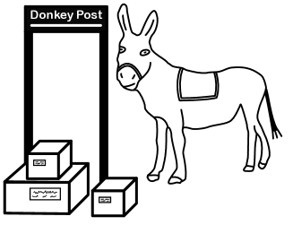
Figure 2.1: How tired is this donkey?

Two-point evaluation model

Consider for a moment the noise free adversarial setting. A number of authors have investigated what changes if the learner is allowed to choose two points $X_{t,1},X_{t,2}\in K$ and observes $f_{t}(X_{t,1})$ and $f_{t}(X_{t,2})$. One might believe that such a modification would have only a mild effect but this is not at all the case. Having access to two evaluations makes the bandit setup behave more like the stochastic optimisation setup just described (Agarwal et al., 2010; Nesterov and Spokoiny, 2017; Duchi et al., 2015).

2.3  Summary table

The table below summarises the past and current situation. The superscript in the function classes indicate whether or not the work only considers the stochastic setting (s).

author	regret	class	notes
Flaxman et al. (2005)	$d^{\frac{1}{2}}\operatorname{diam}(K)^{\frac{1}{2}}n^{\frac{3}{4}}$	$\mathscr{F}_{\tiny{\texttt{b}},\tiny{\texttt{l}}}$	practical
"	$dn^{\frac{5}{6}}$	$\mathscr{F}_{\tiny{\texttt{b}}}$	practical
These notes	$d^{\frac{1}{2}}\vartheta^{\frac{1}{4}}n^{\frac{3}{4}}$	$\mathscr{F}_{\tiny{\texttt{b}}}$	practical
Agarwal et al. (2010)	$d\sqrt{\beta n/\alpha}$	$\mathscr{F}_{\tiny{\texttt{b}},\tiny{\texttt{sm}},\tiny{\texttt{sc}},\tiny{\texttt{u}}}$	practical
Saha and Tewari (2011)	$\vartheta^{\frac{1}{3}}\beta^{\frac{1}{3}}\operatorname{diam}(K)^{\frac{2}{3}}d^{\frac{2}{3}}n^{\frac{2}{3}}$	$\mathscr{F}_{\tiny{\texttt{b}},\tiny{\texttt{sm}}}$	practical
Agarwal et al. (2013)	$\sqrt{n}$	$\mathscr{F}_{\tiny{\texttt{l}}}^{\tiny{\texttt{s}}}$	practical, $d=1$
Agarwal et al. (2013)	$d^{16}\sqrt{n}$	$\mathscr{F}_{\tiny{\texttt{b}},\tiny{\texttt{l}}}^{\tiny{\texttt{s}}}$	poly time
Hazan and Levy (2014)	$d\sqrt{(\vartheta+\beta/\alpha)n}$	$\mathscr{F}_{\tiny{\texttt{b}},\tiny{\texttt{sm}},\tiny{\texttt{sc}}}$	practical
Bubeck et al. (2015)	$\sqrt{n}$	$\mathscr{F}_{\tiny{\texttt{b}}}$	exp time, $d=1$ only
Hazan and Li (2016)	$2^{(d^{4})}\sqrt{n}$	$\mathscr{F}_{\tiny{\texttt{b}}}$	$\log(n)^{\operatorname{poly}(d)}$ running time
Bubeck et al. (2017)	$d^{10.5}\sqrt{n}$	$\mathscr{F}_{\tiny{\texttt{b}}}$	poly time
"	$\sqrt{n}$	$\mathscr{F}_{\tiny{\texttt{b}}}$	practical, $d=1$
Bubeck et al. (2018)	$d^{18}\sqrt{n}$	$\mathscr{F}_{\tiny{\texttt{b}}}$	exp time
Lattimore (2020)	$d^{2.5}\sqrt{n}$	$\mathscr{F}_{\tiny{\texttt{b}}}$	exp time
Ito (2020)	$d\sqrt{\beta n/\alpha}$	$\mathscr{F}_{\tiny{\texttt{b}},\tiny{\texttt{sm}},\tiny{\texttt{sc}}}$	min. away from boundary
"	$d^{1.5}\sqrt{\beta n/\alpha}$	$\mathscr{F}_{\tiny{\texttt{b}},\tiny{\texttt{sm}},\tiny{\texttt{sc}}}$	poly time
Suggala et al. (2021)	$d^{16}\sqrt{n}$	$\mathscr{F}_{\tiny{\texttt{b}},\tiny{\texttt{quad}}}$	poly time
Lattimore and György (2021a)	$d^{4.5}\sqrt{n}$	$\mathscr{F}_{\tiny{\texttt{b}}}^{\tiny{\texttt{s}}}$	ellipsoid method
These notes	$d^{4}\sqrt{n}$	$\mathscr{F}_{\tiny{\texttt{b}}}^{\tiny{\texttt{s}}}$	ellipsoid method
Lattimore and György (2023)	$d^{1.5}\sqrt{n}+\frac{\operatorname{diam}(K)}{\min(1,\varrho)}d\sqrt{n}$	$\mathscr{F}_{\tiny{\texttt{l}},\tiny{\texttt{u}}}^{\tiny{\texttt{s}}}$	practical

2.4  Notes

1. There are some books on zeroth-order optimisation (Larson et al., 2019; Conn et al., 2009, for example). These works focus most of their attention on noise free settings and without a special focus on convexity. Nemirovsky and Yudin (1983) is a more theoretically focussed book with one chapter on zeroth-order methods. there is also a nice short and quite recent survey by Liu et al. (2020).

2. Speaking of non-convexity, zeroth-order methods are also analysed in non-convex settings. Sometimes the objective is still to find the global minimum, but for many non-convex problems this cannot be done efficiently. In such cases one often tries to find a point $x\in K$ such that $\left\|f^{\prime}(x)\right\|$ is small. We only study convex problems here. A recent reference for the non-convex case is the work by Balasubramanian and Ghadimi (2022).

3. There are esoteric settings that are quite interesting and may suit some applications. For example, Bach and Perchet (2016) study a problem where the learner chooses two actions in each round. The learner receives information for only the first action but is evaluated based on the quality of the second. They also study higher levels of smoothness than we consider here.

4. Online learning has for a long time made considerable effort to prove adaptive bounds that yield stronger results when the loss functions are somehow nice or show that the learner adapts to changing environments. Such results have also been commonplace in the standard bandit literature and are starting to appear in the convex bandit literature as well (Zhao et al., 2021; Luo et al., 2022; Wang, 2023)

5. We did not talk much about the efforts focussed on sample complexity or simple regret for the stochastic setting. Jamieson et al. (2012) consider functions in $\mathscr{F}_{\tiny{\texttt{sm}},\tiny{\texttt{sc}}}$ and $K=\mathbb{R}^{d}$ and prove a sample complexity bound of $O(\frac{d^{3}}{\varepsilon^{2}})$ for an algorithm based on coordinate descent with polynomial dependence on the smoothness and strong convexity parameters hidden. Belloni et al. (2015) use an algorithm based on simulated annealing to prove a sample complexity bound of $O(\frac{d^{7.5}}{\varepsilon^{2}})$ for losses in $\mathscr{F}_{\tiny{\texttt{b}}}$. In its current form their algorithm is not suitable for regret minimisation though this minor deficiency may be correctable. Another thing to mention about that work is that the algorithm is robust in the sense that it can (approximately) find minima of functions that are only approximately convex. Slightly earlier Liang et al. (2014) also use a method based on random walks but obtained a worse rate of $O(\frac{d^{14}}{\varepsilon^{2}})$.

Chapter 3  Regularity ()

Bandit convex optimisation is studied on a wide range of structural assumptions on both the loss functions $(f_{t})$ and the constraint set $K$. The purpose of this chapter is to explore the relationships and interactions between the properties like smoothness, strong convexity and Lipschitzness. Besides this we explain two meta algorithms that can be used to bootstrap subsequent algorithms to yield guarantees with fewer assumptions. For example, if you design an algorithm losses in $\mathscr{F}_{\tiny{\texttt{b}},\tiny{\texttt{l}},\tiny{\texttt{sm}},\tiny{\texttt{sc}}}$ and prove a bound on its regret that depends only logarithmically on the diameter, smoothness and strong convexity parameters, then you can use Algorithm 1 to produce an algorithm with the same regret guarantee up to logarithmic factors for losses in $\mathscr{F}_{\tiny{\texttt{b}}}$.

3.1  Convex bodies and the Minkowski functional

A convex set $K\subset\mathbb{R}^{d}$ is a convex body if it is compact and contains a non-empty interior. The latter corresponds to the existence of an $x\in\mathbb{R}^{d}$ and $\varepsilon>0$ such that $x+\mathbb{B}^{d}_{\varepsilon}\subset K$. Given an $x\in\mathbb{R}^{d}$ the Minkowski functional is

$$\pi^{K}_{x}(y)=\inf\left\{t>0:x+\frac{y-x}{t}\in K\right\}\,.$$

Given $x\in K$ and $\varepsilon\in(0,1)$, let

$$K_{x,\varepsilon}=\{\varepsilon x+(1-\varepsilon)y:y\in K\}=\{y\in K:\pi^{K}_{x}(y)\leq 1-\varepsilon\}\,.$$

Lemma 3.1.

Suppose that $x+\mathbb{B}^{d}_{r}\subset K$ and $y\in K_{x,\varepsilon}$. Then $y+\mathbb{B}^{d}_{r\varepsilon}\subset K$.

Proof.

Let $y\in K_{x,\varepsilon}$. By the definition of the Minkowski functional there exists a $z\in K$ such that $y=\varepsilon x+(1-\varepsilon)z$. Since $K$ is convex and $x+\mathbb{B}^{d}_{r}\subset K$, it follows that

$$K \supset\varepsilon(x+\mathbb{B}^{d}_{r})+(1-\varepsilon)z=y+\mathbb{B}^{d}_{\varepsilon r}\,.\qed$$

Figure 3.1: The Minkowski functional and an illustration of $K_{x,\varepsilon}$ for $\varepsilon=\frac{1}{10}$. In this example, $\pi_{x}(y)=\frac{9}{10}$.

3.2  Smoothness and strong convexity

You should check that if $f\in\mathscr{F}_{\tiny{\texttt{sm}},\tiny{\texttt{sc}}}$ and $f$ is twice differentiable, then

$$\alpha\mathds{1}\preceq f^{\prime\prime}(x)\preceq\beta\mathds{1}\text{ for all }x\in\operatorname{int}(K)\,.$$

Besides this, the only properties of smoothness and strong convexity that we need are as follows:

Lemma 3.2.

If $f\in\mathscr{F}$ is $\alpha$-strongly convex, then

$$f(x)\geq f(y)+Df(y)[x-y]+\frac{\alpha}{2}\left\|x-y\right\|^{2}\,.$$

Lemma 3.3.

If $f\in\mathscr{F}$ is $\beta$-smooth and $X$ is a random variable supported in $K$ and $x=\mathbb{E}[X]$. Then,

$$\mathbb{E}[f(X)-f(x)]\leq\frac{\beta}{2}\mathbb{E}\left[\left\|X-x\right\|^{2}\right]\,.$$

Proof.

Let $g(x)=f(x)-\frac{\beta}{2}\left\|X\right\|^{2}$, which by assumption is concave. Then,

$$\mathbb{E}[f(X)-f(x)] =\mathbb{E}[g(X)-g(x)]+\frac{\beta}{2}\mathbb{E}\left[\left\|X\right\|^{2}-\left\|x\right\|^{2}\right]$$

$$\leq\frac{\beta}{2}\mathbb{E}\left[\left\|X\right\|^{2}-\left\|x\right\|^{2}\right] g$$ since is concave

$$=\frac{\beta}{2}\mathbb{E}\left[\left\|X-x\right\|^{2}\right]\,. \mathbb{E}[X]=x$$ since

∎

3.3  Scaling properties

A class of problems is defined by the constraint set $K$ and the function class in which the losses lie (see Definition 1.1) as well as constraints on the adversary (stochastic/non-stochastic) or the noise.. Regardless, we hope you agree that simply changing the scale of the coordinates should not affect the achievable regret. The following proposition describes how the various constants change when the coordinates are scaled.

Proposition 3.4.

Let $f:K\to[0,1]$ be convex and twice differentiable. Define $g(y)=f(x/\gamma)$ and $J=\{\gamma x:x\in K\}$. The following hold:

1. $g:J\to[0,1]$ is convex and twice differentiable.

2. $g^{\prime}(y)=\frac{f^{\prime}(x/\gamma)}{\gamma}$.

3. $g^{\prime\prime}(y)=\frac{f^{\prime\prime}(x/\gamma)}{\gamma^{2}}$.

4. $\operatorname{diam}(J)=\gamma\operatorname{diam}(K)$.

From this we see that the product of the Lipschitz constant and diameter is invariant under scaling. As is the ratio of strong convexity and smoothness parameters. You should always check that various results are compatible with these scaling results in the sense that the regret bound should be invariant to scale if the assumptions permit scaling.

3.4  Convex functions are nearly Lipschitz

Let $f:K\to[0,1]$ be a convex function. Obviously $f$ does not have to be Lipschitz with any constant. For example, $K=[0,1]$ and $f(x)=1-\sqrt{x}$ has gradients that explode as $x\to 0$. But $f$ must be Lipschitz on the interior of $K$ in some sense. You should start by checking that if $A$ is convex and $f$ has directional derivatives and $Df(x)[\eta]\leq L$ for all $x\in A$ and $\eta\in\mathbb{S}^{d-1}_{1}$, then for all $x,y\in A$, $f(x)-f(y)\leq L\left\|x-y\right\|$.

Proposition 3.5.

Suppose that $f\in\mathscr{F}_{\tiny{\texttt{b}}}$ and $x+\mathbb{B}^{d}_{r}\subset K$, then

$$\max_{\eta\in\mathbb{S}^{d-1}_{1}}Df(x)[\eta]\leq\frac{1}{r}\,.$$

Proof.

The assumption that $f$ is convex and bounded in $[0,1]$ on $K$ shows that for any $\eta\in\mathbb{S}^{d-1}_{1}$,

$$1 \geq f(x+r\eta)\geq f(x)+Df(x)[r\eta]\geq Df(y)[r\eta]=rDf(y)[\eta]\,.$$

Therefore $Df(y)[\eta]\leq\frac{1}{r}$. ∎

3.5  Near-optimality on the interior

The observation that convex functions are Lipschitz on a suitable subset of the interior of $K$ suggests that if we want to restrict our attention to Lipschitz functions, then we might pretend that the domain of $f$ is not $K$ but rather a subset. This idea is only fruitful because bounded convex functions are always nearly minimised somewhere on the interior in the following sense. Recall the definition of $K_{x,\varepsilon}$ from Section 3.1.

Proposition 3.6.

Let $K$ be a convex body and $x\in\operatorname{int}(K)$ and $\varepsilon\in(0,1)$. Then

$$\min_{y\in K_{x,\varepsilon}}f(y)\leq\inf_{y\in K}f(y)+\varepsilon\,.$$

Proof.

To begin, the minimum on the left-hand side exists because $K_{x,\varepsilon}$ is a closed subset of the interior of the compact $K$ and hence $K_{x,\varepsilon}$ is a compact subset of $\operatorname{int}(K)$. Furthermore, convex functions are continuous on the interior of their domain, which means that $\sum_{t=1}^{n}f_{t}$ is continuous on $K_{x,\varepsilon}$ and hence has a minimiser. Let $y\in K$. Then $z=(1-\varepsilon)y+\varepsilon\in K_{x,\varepsilon}$ and by convexity, $f(z)\leq(1-\varepsilon)f(y)+\varepsilon f(x)\leq f(y)+\varepsilon$. Taking the infimum over all $y\in K$ completes the proof. ∎

3.6  Extension

Occasionally we need to extend a convex function $f:\mathbb{R}^{d}\to\mathbb{R}\cup\{\infty\}$ with $\operatorname{dom}(f)\subsetneq\mathbb{R}^{d}$ to a convex function $\bar{f}$ such that $\operatorname{dom}(\bar{f})=\mathbb{R}^{d}$ and $f=\bar{f}$ on $\operatorname{dom}(f)$. Sometimes this is not possible. For example, the function defined by

$$f(x)=\begin{cases}1-\sqrt{x}&\text{if }x\geq 0\\ \infty&\text{if }x<0\end{cases}$$

cannot be extended to a convex function with domain $\mathbb{R}$. Fortunately when $f$ is Lipschitz on its domain then an extension to $\mathbb{R}^{d}$ is always possible.

Proposition 3.7.

Suppose that $f:\mathbb{R}^{d}\to\mathbb{R}\cup\{\infty\}$ is Lipschitz on $\operatorname{dom}(f)$. Then there exists a Lipschitz convex function $\bar{f}:\mathbb{R}^{d}\to\mathbb{R}$ with $\bar{f}(x)=f(x)$ for all $x\in\operatorname{dom}(f)$.

Proof.

Simply let $\bar{f}(y)=\sup_{x\in\operatorname{int}(\operatorname{dom}(f))}f(x)+Df(x)[y-x]$. Convexity follows because $\bar{f}$ is the supremum of convex functions. Lipschitzness is left as a simple exercise. ∎

Occasionally it would be convenient to be able to extend $\beta$-smooth functions while preserving $\beta$-smoothness to all of $\mathbb{R}^{d}$. Remarkably this is not possible (Drori, 2018).

3.7  Smoothing

Let $\phi:\mathbb{R}^{d}\to\mathbb{R}$ be the twice differentiable function given by

$$\phi(x) =\frac{\bm{1}_{\mathbb{B}^{d}_{1}}(x)}{C}\left(1-\left\|x\right\|^{2}\right)^{3} C =\int_{\mathbb{B}^{d}_{1}}\left(1-\left\|x\right\|^{2}\right)^{3}\operatorname{d}\!x\,.$$

Note that $\phi$ is the density of a probability measure on $\mathbb{R}^{d}$. Given $\varepsilon>0$, let

$$\phi_{\varepsilon}(x)=\varepsilon^{-d}\phi(x/\varepsilon)\,,$$ (3.1)

which by a change of measure is also a probability density.

Proposition 3.8.

Suppose that $f:\mathbb{R}^{d}\to\mathbb{R}\cup\{\infty\}$ is convex and in $\mathscr{F}_{\tiny{\texttt{l}}}$ and let $g=f*\phi_{\varepsilon}$, which is defined on $\operatorname{dom}(g)=\{x\in\mathbb{R}^{d}:x+\mathbb{B}^{d}_{\varepsilon}\subset\operatorname{cl}(\operatorname{dom}(f))\}$. Then the following hold:

1. $g$ is twice differentiable on $\operatorname{int}(\operatorname{dom}(g))$.

2. $g\in\mathscr{F}_{\tiny{\texttt{l}}}$.

3. $g$ is smooth: $\left\|g^{\prime\prime}(x)\right\|\leq\frac{(d+1)(d+6)}{\varepsilon}$ for all $x\in J$.

4. $\max_{x\in\operatorname{dom}(g)}|f(x)-g(x)|\leq\varepsilon$.

Proof.

Part (a) follows from Young’s convolutional inequality and the fact that $\phi_{\varepsilon}$ is twice differentiable and compactly supported (this is a good exercise). Part (b) is left as an exercise (convolution preserves the Lipschitz property). For part (c), the constant $C$ can be calculated by integrating in polar coordinates:

$$C =\int_{\mathbb{B}^{d}_{1}}\left(1-\left\|x\right\|^{2}\right)^{3}\operatorname{d}\!x$$

$$=d\operatorname{vol}(\mathbb{B}^{d}_{1})\int_{0}^{1}r^{d-1}\left(1-r^{2}\right)^{3}\operatorname{d}\!r$$

$$=\frac{48\operatorname{vol}(\mathbb{B}^{d}_{1})}{(d+2)(d+4)(d+6)}\,.$$

By convexity of the spectral norm and naive calculation:

$$\left\|g^{\prime\prime}(x)\right\| =\left\|\int_{\mathbb{B}^{d}_{\varepsilon}}f(x+u)\phi_{\varepsilon}^{\prime\prime}(x)\operatorname{d}\!x\right\|$$

$$=\left\|\int_{\mathbb{B}^{d}_{\varepsilon}}(f(x+u)-f(x))\phi_{\varepsilon}^{\prime\prime}(x)\operatorname{d}\!x\right\| \int_{\mathbb{B}^{d}_{\varepsilon}}\phi_{\varepsilon}^{\prime\prime}(x)\operatorname{d}\!x=\bm{0}$$

$$\leq\varepsilon\int_{\mathbb{B}^{d}_{\varepsilon}}\left\|\phi_{\varepsilon}^{\prime\prime}(x)\right\|\operatorname{d}\!x f$$ is Lipschitz

$$=\frac{1}{\varepsilon}\int_{\mathbb{B}^{d}_{1}}\left\|\phi^{\prime\prime}(x)\right\|\operatorname{d}\!x$$

$$=\frac{1}{C\varepsilon}\int_{\mathbb{B}^{d}_{1}}\left\|24xx^{\top}(1-\left\|x\right\|^{2})-6\mathds{1}(1-\left\|x\right\|^{2})^{2}\right\|\operatorname{d}\!x$$

$$\leq\frac{1}{C\varepsilon}\int_{\mathbb{B}^{d}_{1}}\left\|24xx^{\top}(1-\left\|x\right\|^{2})+6\mathds{1}(1-\left\|x\right\|^{2})^{2}\right\|\operatorname{d}\!x$$

$$=\frac{(d+1)(d+6)}{\varepsilon}\,,$$

where the final equality follows by substituting the expression for $C$ and integrating in polar coordinates. For part (d), since $f$ is Lipschitz,

$$\left|g(x)-f(x)\right| =\left|\int_{\mathbb{B}^{d}_{\varepsilon}}\left(f(x+u)-f(x)\right)\phi_{\varepsilon}(\operatorname{d}\!u)\right|$$

$$\leq\int_{\mathbb{B}^{d}_{\varepsilon}}\left\|u\right\|\phi_{\varepsilon}(\operatorname{d}\!u)\leq\varepsilon^{,}.\qed$$

3.8  Meta algorithms

We now describe a process which by algorithm designed for losses in $\mathscr{F}_{\tiny{\texttt{b}},\tiny{\texttt{l}},\tiny{\texttt{sm}},\tiny{\texttt{sc}}}$ can be used when the losses $(f_{t})_{t=1}^{n}$ are in fact in $\mathscr{F}_{\tiny{\texttt{b}}}$. The idea is to initialise the learner on a different constraint set $L$ and place an interface between the learner and the environment so that size=,color=red!20!white,]Tor: explain both algorithms and what/why

• From the learner’s perspective they are interacting with a sequence of losses $(g_{t})_{t=1}^{n}:L\to\mathbb{R}$ in $\mathscr{F}_{\tiny{\texttt{b}},\tiny{\texttt{l}},\tiny{\texttt{sm}},\tiny{\texttt{sc}}}$.

• Minimising the losses $(g_{t})_{t=1}^{n}$ on $L$ corresponds to approximately minimising the losses $(f_{t})_{t=1}^{n}$ on $K$.

The next proposition collects all the necessary machinery.

Proposition 3.9.

Let $K$ be a convex body and $f\in\mathscr{F}_{\tiny{\texttt{b}}}$. Suppose that $x+\mathbb{B}^{d}_{r}\subset K$ for some $r>0$ and let $Ty=\frac{1+\varepsilon}{r\varepsilon}(y-x)$ and $J=T(K)$ and

$$g(u)=(1-\varepsilon)\int_{\mathbb{B}^{d}_{\varepsilon}}\bar{f}\left(T^{-1}(u+v)\right)\phi_{\varepsilon}(v)\operatorname{d}\!v+\varepsilon q(u)\,,$$

where $\bar{f}$ is the extension of $f$ defined in the proof of Proposition 3.7 and $q(u)=\frac{1}{2}\left\|u\right\|^{2}/\operatorname{diam}(J)^{2}$.

1. $g$ is Lipschitz on $J$.

2. $g$ is $\beta$-smooth on $\mathbb{R}^{d}$ with $\beta=\frac{(d+1)(d+6)}{\varepsilon}$.

3. $g$ is $\alpha$-strongly on $\mathbb{R}^{d}$ convex with $\alpha=\varepsilon/\operatorname{diam}(J)^{2}$.

4. $g(u)-f(T^{-1}u)\leq\frac{3\varepsilon}{2}$ for all $u\in J$.

5. With $L=\{x\in J:\pi^{J}_{\bm{0}}(x)\leq 1-\varepsilon\}$, $\min_{u\in L}g(u)\leq\min_{y\in K}f(y)+\frac{5\varepsilon}{2}$.

Proof.

Part (a) follows from Proposition 3.5. Part (b) follows from Proposition 3.8. Part (c) is immediate. Part (d) follows from Proposition 3.8 and the definition of $g$. Part (e) follows from Proposition 3.6, which shows that

$$\min_{y\in K}f(y)\leq\min_{y\in K_{x,\varepsilon}}f(y)+\varepsilon\,,$$

and the fact that $L=T(K_{x,\varepsilon})$ and part (d). ∎

Proposition 3.10.

Suppose that $L$ is defined as in Proposition 3.9 and $(f_{t})_{t=1}^{n}$ is a sequence of losses in $\mathscr{F}_{\tiny{\texttt{b}}}$ and

$$g_{t}(u)=(1-\varepsilon)\int_{\mathbb{B}^{d}_{\varepsilon}}f\left(T^{-1}(u+v)\right)\phi_{\varepsilon}(v)\operatorname{d}\!v+\varepsilon q(u)\,.$$

Then, for any sequence $(u_{t})_{t=1}^{n}\in L$ and $(v_{t})_{t=1}^{n}\in\mathbb{B}^{d}_{\varepsilon}$,

$$\max_{x\in K}\sum_{t=1}^{n}\left(f_{t}(T^{-1}(u_{t}+v_{t}))-f_{t}(x)\right)\leq\max_{u\in L}\sum_{t=1}^{n}\left(g_{t}(u_{t})-g_{t}(u)\right)+5\varepsilon n\,.$$

Proof.

Let $x_{t}=T^{-1}(u_{t}+v_{t})$ and $y_{t}=T^{-1}u_{t}$. Since $u_{t}+\mathbb{B}^{d}_{1+\varepsilon}\subset T(K)$, $x_{t}+\mathbb{B}^{d}_{(1+\varepsilon)/\gamma}\subset K$ and by Proposition 3.5,

$$|f_{t}(x_{t})-f_{t}(y_{t})|\leq\frac{\gamma}{1+\varepsilon}\left\|x_{t}-y_{t}\right\|\leq\frac{\varepsilon}{1+\varepsilon}\,.$$

Therefore, by Proposition 3.9(d),

$$f_{t}(T^{-1}(u_{t}+v_{t}))=f_{t}(x_{t})\leq f_{t}(y_{t})+\varepsilon\leq g_{t}(u_{t})+\frac{5\varepsilon}{2}\,.$$

The claim follows from Proposition 3.9(e). ∎

We can now give the meta algorithm that accepts as input a convex bandit optimisation algorithm designed for losses in $\mathscr{F}_{\tiny{\texttt{b}},\tiny{\texttt{l}},\tiny{\texttt{sm}},\tiny{\texttt{sc}}}$ and uses it to solve bandit problems with losses in $\mathscr{F}_{\tiny{\texttt{b}}}$.

⬇

1args: base algorithm $\mathscr{B}$, constraint set $K$

2find $x\in K$ and $0<r\leq R$ such that $x+\mathbb{B}^{d}_{r}\subset K\subset x+\mathbb{B}^{d}_{R}$

3let $\varepsilon=\frac{1}{n}$ and $\gamma=\frac{1+\varepsilon}{r\varepsilon}$ and $T(y)=\gamma(y-x)$

4let $L=(1-\varepsilon)T(K)$ and initialise $\mathscr{B}$ on $L$

5let $q(x)=\frac{\left\|x\right\|^{2}}{2R^{2}}$

6for $t=1$ to $n$

7 request $X_{t}^{L}\in L$ from $\mathscr{B}$

8 sample $V_{t}$ from $\phi_{\varepsilon}$ defined in Eq. 3.1

9 let $X_{t}^{K}=T^{-1}(X_{t}^{L}+V_{t})\in K$

10 observe $Y_{t}^{K}=f_{t}(X_{t}^{K})+\varepsilon_{t}$

11 feed $Y_{t}^{L}=\left(1-\varepsilon\right)Y_{t}^{K}+\varepsilon q(X_{t}^{L})$ to $\mathscr{B}$

Algorithm 1 Meta algorithm

From the learner’s perspective they are observing losses in $\mathscr{F}_{\tiny{\texttt{b}},\tiny{\texttt{l}},\tiny{\texttt{sm}},\tiny{\texttt{sc}}}$ with smoothness, strong convexity and diameter parameters given by

$$\alpha =\frac{r\varepsilon^{2}}{(1+\varepsilon)R^{2}} \beta =\frac{(d+1)(d+6)}{\varepsilon} \operatorname{diam}(L) =\frac{(1+\varepsilon)\operatorname{diam}(K)}{\varepsilon r}$$

The classical application of this transformation is for learners $\mathscr{B}$ with regret for losses in $\mathscr{F}_{\tiny{\texttt{b}},\tiny{\texttt{l}},\tiny{\texttt{sm}},\tiny{\texttt{sc}}}$ of

$$\mathbb{E}[\textrm{Reg}_{n}]=\operatorname{poly}(d,n)\operatorname{polylog}(n,d,\operatorname{diam}(K),\alpha,\beta)\,.$$

By using the meta algorithm $\mathscr{A}$ in Algorithm 1 with base algorithm $\mathscr{B}$ one obtains using Proposition 3.10 a regret for losses in $\mathscr{F}_{\tiny{\texttt{b}}}$ of

$$\mathbb{E}[\textrm{Reg}_{n}]\leq\operatorname{poly}(d,n)\operatorname{polylog}(n,d,\operatorname{diam}(K)/r,R)\,,$$

where the polynomial dependence on $d$ and $n$ is the same. The same statement holds for high probability bounds. An example where this is used is the algorithm introduced in Chapter 10. The scaling of the domain to introduce Lipschitzness is only effective when the regret of the base algorithm depends just logarithmically on the diameter. In Chapter 9 we will see an algorithm with regret analysis for losses in $\mathscr{F}_{\tiny{\texttt{b}},\tiny{\texttt{l}},\tiny{\texttt{sm}},\tiny{\texttt{sc}}}$ with a high probability bound on the regret of

$$\mathbb{P}\left(\textrm{Reg}_{n}\geq\operatorname{poly}(d,n,\operatorname{diam}(K))\operatorname{polylog}(n,d,\alpha,\beta,1/\delta)\right)\leq\delta\,.$$

Such results can be bootstrapped to losses in $\mathscr{F}_{\tiny{\texttt{b}},\tiny{\texttt{l}}}$ by smoothing and adding a small quadratic but skipping the scaling.

⬇

1args: base algorithm $\mathscr{B}$, constraint set $K$

2find $x\in K$ and $r>0$ such that $x+\mathbb{B}^{d}_{r}\subset K\subset x+\mathbb{B}^{d}_{R}$

3let $\varepsilon=\frac{1}{n}$ and $\delta=\frac{1}{n}\min(1,r)$ and let $L=\varepsilon x+(1-\varepsilon)K$

4initialise $\mathscr{B}$ on $L$

5let $q(y)=\frac{\left\|y-x\right\|^{2}}{2R^{2}}$

6for $t=1$ to $n$

7 request $X_{t}^{L}\in L$ from $\mathscr{B}$

8 sample $V_{t}$ from $\phi_{\delta}$ defined in Eq. 3.1

9 let $X_{t}^{K}=X_{t}^{L}+V_{t}\in K$

10 observe $Y_{t}^{K}=f_{t}(X_{t}^{K})+\varepsilon_{t}$

11 feed $Y_{t}^{L}=\left(1-\varepsilon\right)Y_{t}^{K}+\varepsilon q(X_{t}^{L})$ to $\mathscr{B}$

Algorithm 2 Meta algorithm

3.9  Notes

1. Versions of some or all the properties used here have been exploited in a similar fashion by Flaxman et al. (2005); Bubeck et al. (2017); Lattimore (2020) and others.

2. Algorithms 1 and 2 need to find an $x\in K$ and $0<r\leq R$ such that $x+\mathbb{B}^{d}_{r}\subset K\subset x+\mathbb{B}^{d}_{R}$. Such values exist by definition for any convex body but for the algorithms to be computationally efficient we need a procedure for finding them. This depends on how $K$ is represented. Briefly, if $K$ is a polytope or given by separation oracle, then finding $r$ and $R$ that are within $\operatorname{poly}(d)$ factors of the optimal is practical and relatively straightforward. We explain in detail in Appendix C.

3. You should also note that if $K$ is given by a separation oracle, then the $L$ defined in Algorithms 1 and 2 is nothing more than an affine image of $K$ and hence the separation oracle for $K$ can be used to defined a separation oracle for $L$.

Chapter 4  Bisection in one dimension

We start with a simple but instructive algorithm for the one-dimensional stochastic setting. Throughout this chapter we assume that:

1. $d=1$ and $K$ is a non-empty interval; and

2. The losses are stochastic: $f_{t}=f$ for all $t$; and

3. The losses are Lipschitz: $f\in\mathscr{F}_{\tiny{\texttt{l}}}$.

4.1  Bisection method without noise

The bisection method for deterministic zeroth-order convex optimisation is very simple.

⬇

1let $K_{1}=K$

2for $k=1$ to $\infty$:

3 let $x=\min K_{k}$ and $y=\max K_{k}$

4 let $x_{0}=\frac{1}{3}x+\frac{2}{3}y$, $x_{1}=\frac{2}{3}x+\frac{1}{3}y$

5 if $f(x_{1})\geq f(x_{0})$: then $K_{k+1}=[x,x_{1}]$

6 else: $K_{k+1}=[x_{0},y]$

Algorithm 3 Bisection method without noise

Theorem 4.1.

Let $x_{\star}=\operatornamewithlimits{arg\,min}_{x\in K}f(x)$. Then the following holds for the sequence of intervals $(K_{k})_{k=1}^{\infty}$ produced by Algorithm 3:

1. $x_{\star}\in K_{k}$; and

2. $\operatorname{vol}(K_{k})\leq\left(\frac{2}{3}\right)^{k-1}\operatorname{vol}(K)$.

Part (a) follows from convexity of $f$ while part (b) follows from the definition of the algorithm. By the assumption that $f$ is Lipschitz, for all $x\in K_{k}$, $f(x)\leq f(x_{\star})+(\frac{2}{3})^{k-1}\operatorname{vol}(K)$. Therefore all points in $K_{k}$ are near-optimal when $k$ is only moderately large.

4.2  Bisection method with noise

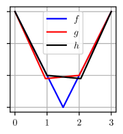
Figure 4.1:

The generalisation of the bisection method to noisy optimisation is surprisingly subtle. While Algorithm 3 divides the current interval into three blocks, in the noisy setting it turns out that four blocks are necessary. The situation is best illustrated by an example. Suppose you have noisy (and therefore only approximate) estimates of the loss at all of $x\in\{0,1,2,3\}$. Notice how all three convex functions $f,g$ and $h$ have very similar values at these points but the minimiser could be in any of $(0,1)$, $(1,2)$ or $(2,3)$. Hence it will take many samples to identify which function is the truth. Even worse, if the real function is $f$, then you are paying considerable regret while trying to identify the region where the minimiser lies. The example illustrates the problem of exploring efficiently. A good exploration strategy will ensure that if the regret is large, then the information gain about the identity/location of a near-minimiser is also large. The exploration strategy in Figure 4.1 is not good. The example also illustrates the challenges of generalising methods designed for deterministic zeroth-order optimisation to stochastic zeroth-order optimisation. Fundamentally the problem is one of stability. Algorithm 3 is not a stable algorithm in the sense that small perturbation of its observations can dramatically change its behaviour.

We decompose the bisection method for stochastic convex optimisation into two algorithms. The first accepts as input an interval and interacts with the loss for a number of rounds. Eventually it outputs a new interval such that with high probability all of the following hold:

• The minimiser of the loss is contained in the output interval.

• The new interval is three quarters as large as the input interval.

• The regret suffered during the interaction is controlled.

⬇

1args: $K=[x,y]$, $\delta\in(0,1)$

2$x_{0}=\frac{1}{4}x+\frac{3}{4}y$, $x_{1}=\frac{1}{2}x+\frac{1}{2}y$, $x_{2}=\frac{3}{4}x+\frac{1}{4}y$

3for $t=1$ to $n$:

4 $c_{t}=\sqrt{\frac{6}{t}\log\left(\frac{n}{\delta}\right)}$

5 let $X_{t}=x_{t\bmod 3}$ and observe $Y_{t}=f(X_{t})+\varepsilon_{t}$

6 if $t\equiv 0\mod 3$:

7 let $\hat{f}_{t}(x_{k})=\frac{3}{t}\sum_{u=1}^{t}\bm{1}(u\equiv k\mod 3)Y_{u}$

8 if $\hat{f}_{t}(x_{2})-\hat{f}_{t}(x_{1})\geq c_{t}$: return $[x,x_{2}]$

9 if $\hat{f}_{t}(x_{0})-\hat{f}_{t}(x_{1})\geq c_{t}$: return $[x_{0},y]$

Algorithm 4 Bisection episode

Proposition 4.2.

Let $[z,w]$ be the interval returned by the algorithm and

$$\Delta=\frac{1}{3}\left[f(x_{0})+f(x_{1})+f(x_{2})\right]-f(x_{\star})\,.$$

With probability at least $1-\delta$ the following both hold:

1. The algorithm either does not return an interval or $x_{\star}\in[z,w]$; and

2. The number of queries to the zeroth-order oracle is at most

   $$3+\frac{100}{\Delta^{2}}\log\left(\frac{n}{\delta}\right)\,.$$

Proof.

By convexity, $\max(f(x_{0}),f(x_{2}))\geq f(x_{1})$. Assume without loss of generality for the remainder of the proof that $f(x_{2})\geq f(x_{1})$ and let $\theta=f(x_{2})-f(x_{1})$. By concentration of measure (Theorem B.6) and a union bound, $\mathbb{P}(G)\geq 1-\delta$, where $G=G_{12}\cup G_{32}$ with

$$G_{12} =\bigcup_{t=1}^{n}\left\{\left|\hat{f}_{t}(x_{1})-\hat{f}_{t}(x_{2})-f(x_{1})+f(x_{2})\right|\leq c_{t}\right\}$$

$$G_{32} =\bigcup_{t=1}^{n}\left\{\left|\hat{f}_{t}(x_{3})-\hat{f}_{t}(x_{2})-f(x_{3})+f(x_{2})\right|\leq c_{t}\right\}\,.$$

Suppose now that $G$ holds. We claim that $\theta\geq\frac{1}{2}\Delta$. Viewing $x_{0},x_{1},x_{2}$ and $f(x_{0})$, $f(x_{1})$, $f(x_{2})$ as fixed, the question is how small can $f(x_{\star})$ be? There are two cases.

1. $[f(x_{0})\leq f(x_{1})]$. Here the smallest possible $f(x_{\star})$ is when $x_{\star}=x$ and by convexity:
   ➳ $f(x_{2})-f(x_{\star})\leq 3\theta$; and ➳ $f(x_{1})-f(x_{\star})\leq 2\theta$; and ➳ $f(x_{0})-f(x_{\star})\leq\theta$.

2. $[f(x_{0})>f(x_{1})]$: Here the smallest value of $f(x_{\star})$ does not exist but the limiting case is when $x_{\star}\to x_{0}$ from the right and
   ➳ $f(x_{2})-f(x_{\star})\leq 2\theta$; and ➳ $f(x_{1})-f(x_{\star})\leq\theta$; and ➳ $f(x_{0})-f(x_{\star})\leq 2\theta$.

In both cases the result follows from the definition of $\Delta$. We are now in a position to establish the claims of the theorem. For part (a). By assumption $f(x_{2})\geq f(x_{1})$ and hence $x_{\star}$ cannot be in $[x_{2},y]$. The algorithm cannot do any wrong if $x_{\star}\in[x_{0},x_{2}]$. Suppose that $x_{\star}\in[x,x_{0}]$. By convexity $f(x_{0})\leq f(x_{1})$ and hence on $G$,

$$\hat{f}_{t}(x_{0})-\hat{f}_{t}(x_{1})<f(x_{0})-f(x_{1})+c_{t}\leq c_{t}\,,$$

which means the algorithm does not return $[x,x_{2}]$. For part (b), suppose that $c_{t}\leq\frac{1}{2}\theta$. Then, on event $G$,

$$\hat{f}_{t}(x_{2})-\hat{f}_{t}(x_{1})\geq f(x_{2})-f(x_{1})-c_{t}=\theta-c_{t}\geq c_{t}\,,$$

which means the algorithm halts. Since $\theta\geq\frac{1}{2}\Delta$, it follows that on $G$ the algorithm halts once $c_{t}\leq\frac{1}{4}\Delta$. The claim follows from the definition of $c_{t}$. ∎

⬇

1args: $K=[x,y]$

2let $K_{1}=[x,y]$

3for $k=1$ to $\infty$

4 run Algorithm 4 with input $K_{k}$

5 receive $K_{k+1}$ as the output

Algorithm 5 Bisection method

Theorem 4.3.

With probability at least $1-n\delta$, the regret of Algorithm 5 is bounded by

$$\textrm{Reg}_{n} \leq 13\operatorname{vol}(K)+10\sqrt{n\log\left(\frac{n}{\delta}\right)\left(1+\frac{\log(n)}{\log(4/3)}\right)}\,.$$

Proof.

Let $K_{k}=[x_{k},y_{k}]$ and

$$\Delta_{k}=\frac{1}{3}\left[f\left(\frac{1}{4}x_{k}+\frac{3}{4}y_{k}\right)+f\left(\frac{1}{2}x_{k}+\frac{1}{2}y_{k}\right)+f\left(\frac{3}{4}x_{k}+\frac{1}{4}y_{k}\right)\right]-f(x_{\star})\,.$$

Since $f$ is Lipschitz, provided that $x_{\star}\in K_{k}$ it holds that $\Delta_{k}\leq y_{k}-x_{k}\leq(\frac{3}{4})^{k-1}\operatorname{vol}(K)$. Since every call to Algorithm 4 makes at least three queries to $f$, there very naively cannot be more than $n$ calls to Algorithm 4. Hence, by a union bound and Proposition 4.2, with probability at least $1-n\delta$, every call made to Algorithm 4 either ends with the budget of queries being exhausted or returns a new interval containing the optimum after at most $n_{k}$ queries with

$$n_{k}\leq 3+\frac{100}{\Delta_{k}^{2}}\log\left(\frac{n}{\delta}\right)\,.$$

Assume this good event occurs and note that $\Delta_{k}\leq\frac{\operatorname{vol}(K)}{n}$ for $k\geq k_{\star}=1+\frac{\log(n)}{\log(4/3)}$. Therefore, with probability at least $1-n\delta$,

$$\textrm{Reg}_{n} =\sum_{t=1}^{n}\left(f(X_{t})-f(x_{\star})\right)$$

$$\leq\operatorname{vol}(K)+\sum_{k=1}^{\infty}\bm{1}(k<k_{\star})n_{k}\Delta_{k}$$

$$\leq\operatorname{vol}(K)+3\sum_{k=1}^{\infty}\left(\frac{3}{4}\right)^{k-1}\operatorname{vol}(K)+10\sum_{k=1}^{\infty}\bm{1}(k<k_{\star})\sqrt{n_{k}\log\left(\frac{n}{\delta}\right)}$$

$$\leq 13\operatorname{vol}(K)+10\sqrt{n\log\left(\frac{n}{\delta}\right)\left(1+\frac{\log(n)}{\log(4/3)}\right)}\,.\qed$$

4.3  Notes

1. Algorithm 4 is due to Agarwal et al. (2011). The basic principle behind the bisection method is that the volume of $K_{k}$ is guaranteed to decrease rapidly with the number of iterations. Generalising this method to higher dimensions is rather non-trivial. Agarwal et al. (2011) and Lattimore and György (2021a) both used algorithms based on the ellipsoid method, which we cover in Chapter 10.

2. Algorithm 4 works with no assumptions on $f$ beyond convexity and Lipschitzness and ensures $O(\sqrt{n}\log(n))$ regret in the stochastic setting. The algorithm is distinct from all others in these notes because its regret depends only very weakly on the range of the loss function. This is what one should expect from algorithms in the stochastic setting where the magnitude of the noise rather than the losses should determine the regret, as it does for finite-armed bandits.

3. There are various ways to refine Algorithm 3 for the deterministic case that better exploit convexity (Orseau and Hutter, 2023). These ideas have not yet been exploited in the noisy (bandit) setting. Bisection-based methods seem fast and require just $O(\log(1/\varepsilon))$ queries to the zeroth-order oracle to find an $\varepsilon$-optimal point. Remarkably, for suitably well-behaved functions Newton’s method is exponentially faster with sample complexity $O(\log\log(1/\varepsilon))$.

4. Cheshire et al. (2020) construct a more sophisticated algorithm for which the expected simple regret is

   $$\mathbb{E}[\textrm{sReg}_{n}]=O\left(\sqrt{\frac{\log\log(n)}{n}}\right)\,,$$

   which they show is optimal. By applying Eq. 1.2 with Algorithm 5 and $\delta=1/n^{2}$ one obtains a worse bound of

   $$\mathbb{E}[\textrm{sReg}_{n}]=O\left(\frac{\log(n)}{\sqrt{n}}\right)\,.$$

   Exactly what the logarithmic dependence should be for the expected regret (cumulative rather than simple) seems to be unknown.

Chapter 5  Gradient descent

Throughout this chapter we assume that

1. $\mathbb{B}^{d}_{1}\subset K$; and

2. The loss functions $(f_{t})_{t=1}^{n}$ are in $\mathscr{F}_{\tiny{\texttt{b}},\tiny{\texttt{l}}}$; and

3. There is no noise: $\varepsilon_{t}=0$ almost surely.

That is, the constraint set contains the euclidean ball, the losses are bounded and Lipschitz and there is no noise. In contrast to the previous chapter, the setting is now adversarial.

5.1  Gradient descent

Gradient descent incrementally computes a sequence of iterates $(x_{t})_{t=1}^{n}$ with $x_{t+1}$ computed by taking a gradient step from $x_{t}$. The euclidean projection onto $K$ is $\Pi_{K}(x)=\operatornamewithlimits{arg\,min}_{y\in K}\left\|x-y\right\|$. The abstract algorithm is given below.

⬇

1args: learning rate $\eta>0$

2initialise $x_{1}\in K$

3for $t=1$ to $n$

4 sample $X_{t}$ from some distribution based on $x_{t}$

5 observe $Y_{t}$

6 compute gradient estimate $g_{t}$ using $x_{t}$, $X_{t}$ and $Y_{t}$

7 update $x_{t+1}=\Pi_{K}(x_{t}-\eta g_{t})$

Algorithm 6 Abstract gradient descent

Importantly, the algorithm does not evaluate the loss function at $x_{t}$ but rather at some random point $X_{t}$ and the distribution of this point has not been specified yet. We have rather informally written that $X_{t}$ should be based on $x_{t}$, by which we mean that

$$\mathbb{P}(X_{t}\in A|\mathscr{F}_{t-1})=\nu(A,x_{t})$$

for some probability kernel $\nu:\mathscr{B}(K)\times K\to[0,1]$. The kernel $\nu$ determines how the algorithm explores. The gradient estimate $g_{t}$ is usually not an estimate of $f^{\prime}_{t}(x)$, which may well not even exist. Instead it is an estimate of the gradient of some surrogate loss function $s_{t}$ that is close to $f_{t}$ in a certain sense. We return to the problem of defining the exploration kernel, surrogate and gradient estimates momentarily. Before that we give some details about gradient descent. The analysis of gradient descent at our disposal from the online learning literature yields a bound on the regret relative to the linear losses defined by the gradient estimates $g_{t}$. Specifically, we have the following theorem:

Theorem 5.1.

For any $x\in K$,

$$\widehat{\textrm{Reg}}_{n}(x)\triangleq\sum_{t=1}^{n}\left\langle g_{t},x_{t}-x\right\rangle\leq\frac{\operatorname{diam}(K)^{2}}{2\eta}+\frac{\eta}{2}\sum_{t=1}^{n}\left\|g_{t}\right\|^{2}\,.$$

Proof.

Let $x\in K$. Then,

$$\frac{1}{2}\left\|x_{t+1}-x\right\|^{2} =\frac{1}{2}\left\|\Pi_{K}(x_{t}-\eta g_{t})-x\right\|^{2}$$

$$\leq\frac{1}{2}\left\|x_{t}-x-\eta g_{t}\right\|^{2}$$

$$=\frac{1}{2}\left\|x_{t}-x\right\|^{2}+\frac{\eta^{2}}{2}\left\|g_{t}\right\|^{2}-\eta\left\langle g_{t},x_{t}-x\right\rangle\,.$$

Rearranging shows that

$$\widehat{\textrm{Reg}}_{n}(x) =\sum_{t=1}^{n}\left\langle g_{t},x_{t}-x\right\rangle$$

$$\leq\sum_{t=1}^{n}\left[\frac{\eta}{2}\left\|g_{t}\right\|^{2}+\frac{1}{2\eta}\left\|x_{t}-x\right\|^{2}-\frac{1}{2\eta}\left\|x_{t+1}-x\right\|^{2}\right]$$

$$\leq\frac{1}{2\eta}\left\|x_{1}-x\right\|^{2}+\frac{\eta}{2}\sum_{t=1}^{n}\left\|g_{t}\right\|^{2}$$

$$\leq\frac{\operatorname{diam}(K)^{2}}{2\eta}+\frac{\eta}{2}\sum_{t=1}^{n}\left\|g_{t}\right\|^{2}\,.\qed$$

What conditions are needed on the gradients $(g_{t})_{t=1}^{n}$ if we want to bound the actual regret in terms of $\widehat{\textrm{Reg}}_{n}$? We have

$$\mathbb{E}[\textrm{Reg}_{n}] =\max_{x\in K}\mathbb{E}\left[\sum_{t=1}^{n}f_{t}(X_{t})-f_{t}(x)\right]$$

$$=\max_{x\in K}\mathbb{E}\left[\sum_{t=1}^{n}\mathbb{E}_{t-1}[f_{t}(X_{t})]-f_{t}(x)\right]$$

$$\stackrel{{\scriptstyle(\dagger)}}{{\lesssim}}\max_{x\in K}\mathbb{E}\left[\sum_{t=1}^{n}\left\langle\mathbb{E}_{t-1}[g_{t}],x_{t}-x\right\rangle\right]$$

$$=\max_{x\in K}\mathbb{E}\left[\sum_{t=1}^{n}\left\langle g_{t},x_{t}-x\right\rangle\right]=\max_{x\in K}\mathbb{E}\left[\widehat{\textrm{Reg}}_{n}(x)\right]$$

The question is how can we ensure that $(\dagger)$ holds? Since $x_{\star}$ is not known, the most obvious way is to choose $g_{t}$ in such a way that for all $x\in K$,

$$\mathbb{E}_{t-1}[f_{t}(X_{t})]-f_{t}(x)\lesssim\left\langle\mathbb{E}_{t-1}[g_{t}],x_{t}-x\right\rangle\,.$$

Furthermore, to bound $\mathbb{E}[\widehat{\textrm{Reg}}_{n}]$ we need to bound $\mathbb{E}_{t-1}[\|g_{t}\|^{2}]$. Summarising, a surrogate gradient estimate $g_{t}$ will yield a good regret bound if:

1. $\mathbb{E}_{t-1}[f_{t}(X_{t})]-f_{t}(x)\lesssim\left\langle\mathbb{E}_{t-1}[g_{t}],x_{t}-x\right\rangle$ for all $x\in K$; and

2. $\mathbb{E}_{t-1}[\|g_{t}\|^{2}]$ is small.

Does such an estimator exist? Read on!

5.2  Spherical smoothing

Let $x\in K$ and $f\in\mathscr{F}_{\tiny{\texttt{b}},\tiny{\texttt{l}}}$. Our algorithm will play some action $X$ that is a random variable and observe $Y=f(X)$. We want a gradient estimator $g$ that is a function of $X$ and $Y$ such that

1. $\mathbb{E}[f(X)]-f(y)\lesssim\left\langle\mathbb{E}[g],x-y\right\rangle$ for all $y\in K$; and

2. $\mathbb{E}[\|g\|^{2}]$ is small.

A simple and beautiful estimator is based on Stoke’s theorem. Let $r\in(0,1)$ be a precision parameter and define $s$ as the convolution between $f$ and a uniform distribution on $\mathbb{B}^{d}_{r}$. That is,

$$s(x)=\frac{1}{\operatorname{vol}(\mathbb{B}^{d}_{r})}\int_{\mathbb{B}^{d}_{r}}f(x+u)\operatorname{d}\!u\,.$$

Some examples are plotted in Figure 5.1. The function $s$ is convex because it is the convolution of convex functions. We have to be careful about the domain of $s$. Because $f$ is only defined on $K$, the surrogate $s$ is only defined on

$$J=\{x\in K:x+\mathbb{B}^{d}_{r}\subset K\}\,.$$

You should check that $J$ is convex and since $r\in(0,1)$, $J$ is non-empty by the assumption that $\mathbb{B}^{d}_{1}\subset K$. By Stoke’s theorem, the gradient of $s$ at $x$ is

$$s^{\prime}(x)=\frac{1}{\operatorname{vol}(\mathbb{B}^{d}_{r})}\int_{\mathbb{B}^{d}_{r}}f^{\prime}(x+u)\operatorname{d}\!u=\frac{d}{r}\left[\frac{1}{\operatorname{vol}(\mathbb{S}^{d-1}_{r})}\int_{\mathbb{S}^{d-1}_{r}}f(x+u)\frac{u}{r}\right]\operatorname{d}\!u\,,$$

where we also used the fact from Proposition A.1 that $\operatorname{vol}(\mathbb{S}^{d-1}_{r})/\operatorname{vol}(\mathbb{B}^{d}_{r})=\frac{d}{r}$. We estimate $s^{\prime}(x)$ by sampling $U$ uniformly from $\mathbb{S}^{d-1}_{r}$, letting $X=x+U$ and defining the surrogate gradient estimate by

$$g=\frac{dYU}{r^{2}}\,,$$

which has expectation $\mathbb{E}[g]=s^{\prime}(x)$. How well does this estimator satisfy our criteria? Well, $s$ is convex so

$$\left\langle\mathbb{E}[g],x-y\right\rangle=\left\langle s^{\prime}(x),x-y\right\rangle\geq s(x)-s(y)\geq\mathbb{E}[f(X)]-f(y)-2r\,,$$ (5.1)

where the final inequality follows from the definition of $s$ and the fact that $f$ is Lipschitz. This seems fairly promising. When $r$ is small, then (a) above is indeed satisfied. Slightly less promising is that

$$\mathbb{E}[\left\|g\right\|^{2}]=\frac{d^{2}}{r^{2}}\mathbb{E}[Y^{2}]=\frac{d^{2}}{r^{2}}\mathbb{E}[f(X)^{2}]\leq\frac{d^{2}}{r^{2}}\,,$$ (5.2)

where we used the fact that $\left\|U\right\|=r$ and the assumption that $f\in\mathscr{F}_{\tiny{\texttt{b}}}$ is bounded on $K$. The situation is at a standoff. To satisfy (a) we need $r$ to be fairly small, but then $\mathbb{E}[\left\|g\right\|^{2}]$ will not be that small. Nevertheless, enough has been done to make progress.

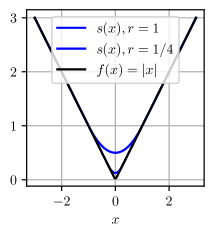
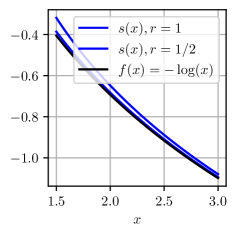
Figure 5.1: The smoothed surrogates for different functions and precisions. Because of convexity the surrogate function is always an upper bound on the original function. Notice how much better the approximation is for $-\log(x)$, which on the interval considered is much smoother than $|x|$.

5.3  Algorithm and regret analysis

The surrogate and its gradient estimator can be cleanly inserted into stochastic gradient descent to obtain the following simple algorithm for bandit convex optimisation.

⬇

1args: learning rate $\eta>0$ and precision $r\in(0,1)$

2initialise $x_{1}\in J=\{x\in K:x+\mathbb{B}^{d}_{r}\subset K\}$

3for $t=1$ to $n$

4 sample $U_{t}$ uniformly from $\mathbb{S}^{d-1}_{r}$ and play $X_{t}=x_{t}+U_{t}$

5 compute gradient estimate $g_{t}=\frac{dY_{t}U_{t}}{r^{2}}$

6 update $x_{t+1}=\Pi_{J}(x_{t}-\eta g_{t})$.

Algorithm 7 Bandit gradient descent

Theorem 5.2.

Suppose that

$$\eta =2^{-\frac{1}{2}}d^{-\frac{1}{2}}\operatorname{diam}(K)^{\frac{3}{2}}n^{-\frac{3}{4}} r =2^{-\frac{1}{2}}d^{\frac{1}{2}}\operatorname{diam}(K)^{\frac{1}{2}}n^{-\frac{1}{4}}\,.$$

Then the expected regret of Algorithm 7 is bounded by

$$\mathbb{E}[\textrm{Reg}_{n}]\leq\sqrt{8}\operatorname{diam}(K)^{\frac{1}{2}}d^{\frac{1}{2}}n^{\frac{3}{4}}$$

Proof.

The surrogate in round $t$ is

$$s_{t}(x)=\frac{1}{\operatorname{vol}(\mathbb{B}^{d}_{r})}\int_{\mathbb{B}^{d}_{r}}f_{t}(x+u)\operatorname{d}\!u\,.$$

Since the losses are in $\mathscr{F}_{\tiny{\texttt{b}},\tiny{\texttt{l}}}$ and hence Lipschitz,

$$\min_{x\in J}\sum_{t=1}^{n}f_{t}(x)\leq rn+\min_{x\in K}\sum_{t=1}^{n}f_{t}(x)$$

Therefore, letting $x_{\star}=\operatornamewithlimits{arg\,min}_{x\in J}\sum_{t=1}^{n}f_{t}(x)$,

$$\mathbb{E}[\textrm{Reg}_{n}] =\max_{x\in K}\mathbb{E}\left[\sum_{t=1}^{n}(f_{t}(X_{t})-f_{t}(x))\right]$$

$$\leq rn+\mathbb{E}\left[\sum_{t=1}^{n}(f_{t}(X_{t})-f_{t}(x_{\star}))\right]$$

$$=3rn+\mathbb{E}\left[\sum_{t=1}^{n}\left\langle g_{t},x_{t}-x_{\star}\right\rangle\right]\,.$$ By Eq. 5.1

By Theorem 5.2,

$$\mathbb{E}\left[\sum_{t=1}^{n}\left\langle g_{t},x_{t}-x_{\star}\right\rangle\right] \leq\frac{\operatorname{diam}(K)^{2}}{2\eta}+\frac{\eta}{2}\mathbb{E}\left[\sum_{t=1}^{n}\left\|g_{t}\right\|^{2}\right]$$

$$\leq\frac{\operatorname{diam}(K)^{2}}{2\eta}+\frac{\eta nd^{2}}{2r^{2}}\,.$$ By Eq. 5.2

Combining shows that

$$\mathbb{E}[\textrm{Reg}_{n}]\leq\frac{\operatorname{diam}(K)^{2}}{2\eta}+\frac{\eta nd^{2}}{2r^{2}}+3nr\,.$$

The claim follows by substituting the constants (see Lemma A.3). ∎

5.4  Notes

1. Theorem 5.1 is due to Zinkevich (2003).

2. Algorithm 7 essentially appears in the independent works by Flaxman et al. (2005) and Kleinberg (2005). The algorithm continues to work without Lipschitzness but the regret increases to $O(\operatorname{cond}(K)^{1/2}d^{1/2}n^{5/6})$ or $O(dn^{5/6})$ as explained by Flaxman et al. (2005).

3. As far as we know the spherical smoothing estimator was introduced by Nemirovsky and Yudin (1983) who used it as a first-order oracle to prove sample complexity bounds. Omitting dependence on everything except accuracy, they proved a sample complexity bound of $O(1/\varepsilon^{4})$. Nemirovsky and Yudin (1983) also noticed that smoothness increases the performance of the spherical estimator, which we explain in Chapter 6. size=,color=red!20!white,]Tor: Check this. How do they handle constraints?

4. We did not say much about computation. The only complicated part is computing the projections, the hardness of which depends on how $K$ is represented. Note the algorithm does not project onto $K$ but rather $J=\{x\in K:x+\mathbb{B}^{d}_{r}\subset K\}$. Practically speaking it is probably preferable to project onto $K_{r}=\{(1-r)x:x\in K\}$. By assumption $K$ contains the unit radius euclidean ball and therefore $K_{r}\subset J$. But by Proposition 3.6, $K_{r}$ is large enough that $\min_{x\in K_{r}}\sum_{t=1}^{n}f_{t}(x)\leq nr+\min_{x\in K}\sum_{t=1}^{n}f_{t}(x)$. As we discuss briefly in Appendix C, $K_{r}$ inherits many nice computation properties from $K$ and polynomial time euclidean projection is often possible.

5. Garber and Kretzu (2022) show there are alternative ways to keep the iterates inside the constraint set. They assume that $\mathbb{B}^{d}_{\delta}\subset K$ for some $\delta>0$ and design gradient-descent-based algorithms for which the regret more-or-less matches Theorem 5.2 and that need either $O(n)$ queries to a linear optimisation oracle or $O(n)$ queries to a separation oracle.

Chapter 6  Self-concordant regularisation

The algorithm based on gradient descent in the previous chapter is simple and computationally efficient. There are two limitations, however.

• We needed to assume the losses were Lipschitz and the regret depended polynomially on the diameter.

• Exploiting smoothness and/or strong convexity is not straightforward due to boundary effects.

Both limitations will be removed using follow the regularised leader and the beautiful machinery of self-concordant barriers. Globally in this chapter we make the following assumptions:

1. There is no noise: $\varepsilon_{t}=0$ for all $t$.

2. The losses are bounded: $f_{t}\in\mathscr{F}_{\tiny{\texttt{b}}}$ for all $t$.

6.1  Self-concordant barriers

A three times differentiable convex function $R:K\to\mathbb{R}\cup\{\infty\}$ is self-concordant if

1. $D^{3}R(x)[h,h,h]\leq 2(D^{2}R(x)[h,h])^{3/2}$ for all $h\in\mathbb{R}^{d}$; and

2. $R$ is a barrier: $R(x_{t})\to\infty$ whenever $x_{t}\to\partial K$.

It is called a $\vartheta$-self-concordant barrier if additionally:

1. $DR(x)[h]\leq\sqrt{\vartheta D^{2}R(x)[h,h]}$ where $\vartheta$ is a (hopefully small) positive real value.

The local norm at $x\in K$ associated with $R$ is $\left\|h\right\|_{x}=\left\|h\right\|_{R^{\prime\prime}(x)}$ and its dual is $\left\|h\right\|_{x\star}=\left\|h\right\|_{R^{\prime\prime}(x)^{-1}}$. The Dikin ellipsoid of radius $r$ at $x$ is

$$E^{x}_{r}=\{y:\left\|y-x\right\|_{x}\leq r\}\,.$$

We collect the following facts about $\vartheta$-self-concordant barriers:

Lemma 6.1.

Suppose that $R$ is self-concordant on $K$, then

1. The Dikin ellipsoid is contained in $K$: $E^{x}_{1}\subset K$ for all $x\in\operatorname{int}(K)$.

2. For all $x\in\operatorname{int}(K)$ and $y\in K$,

   $$R(y)\geq R(x)+\left\langle R^{\prime}(x),y-x\right\rangle+\rho(-\left\|x-y\right\|_{x})$$

   with $\rho(s)=-\log(1-s)-s$.

3. $\operatorname{tr}(R^{\prime\prime}(x)^{-1})\leq d\operatorname{diam}(K)^{2}$ for all $x\in\operatorname{int}(K)$.

Suppose additionally that $R$ is $\vartheta$-self-concordant, then

1. $R(y)\leq R(x)-\vartheta\log\left(1-\pi^{K}_{x}(y)\right)$ for all $x,y\in\operatorname{int}(K)$.

Proof.

() Part (a) appears as Equation (2.2) in the notes by Nemirovski (1996). Part (b) is Equation (2.4) in the same notes. Part (c) follows from Part (a). To see why, let $\eta\in\mathbb{S}^{d-1}_{1}$ and notice that $y=x+R^{\prime\prime}(x)^{-1/2}\eta\in E^{x}_{1}\subset K$. Therefore $\left\|\eta\right\|_{R^{\prime\prime}(x)^{-1}}=\left\|x-y\right\|\leq\operatorname{diam}(K)$. The result follows because

$$\operatorname{tr}(R^{\prime\prime}(x)^{-1})=\sum_{k=1}^{d}\left\|e_{k}\right\|^{2}_{R^{\prime\prime}(x)^{-1}}$$

with $(e_{k})_{k=1}^{d}$ the standard basis vectors. Part (d) appears as Equation (3.7) in the notes by Nemirovski (1996). ∎

Figure 6.1: Dikin ellpsoids for a polytope and the ball using the barriers in Note ➳ ‣ (c).

Lemma 6.2.

Suppose that $\Phi:K\to\mathbb{R}$ is self-concordant and $x=\operatornamewithlimits{arg\,min}_{z\in K}\Phi(x)$ and $\left\|\Phi^{\prime}(y)\right\|_{y\star}\leq\frac{1}{2}$, then $\Phi(y)-\Phi(x)\leq\left\|\Phi^{\prime}(y)\right\|^{2}_{y\star}$.

Proof.

() Abbreviate $g=\Phi^{\prime}(y)$. Then,

$$\Phi(x) \geq\Phi(y)+\left\langle g,x-y\right\rangle+\rho(-\left\|x-y\right\|_{y})$$ Lemma 6.1(b)

$$\geq\Phi(y)-\left\|g\right\|_{y\star}\left\|x-y\right\|_{y}+\rho(-\left\|x-y\right\|_{y})$$ Cauchy-Schwarz

Therefore,

$$\Phi(y) \leq\Phi(x)+\left\|g\right\|_{y\star}\left\|x-y\right\|_{y}-\rho(-\left\|x-y\right\|_{y})$$

$$\leq\Phi(x)+\max_{r\geq 0}\left[r\left\|g\right\|_{y\star}-\rho(-r)\right]$$

$$=\Phi(x)-\log\left[1-\left\|g\right\|_{y\star}\right]-\left\|g\right\|_{y\star}$$

$$\leq\Phi(x)+\left\|g\right\|_{y\star}^{2}\,.$$

where in the final inequality we used the elementary and naive inequality: $-\log(1-t)-t\leq t^{2}$ for $t\leq\frac{1}{2}$. ∎

6.2  Follow the regularised leader

Follow the regularised leader can be viewed as a generalisation of gradient descent, which for bandits has the following abstract form. Like gradient descent, follow the regularised leader maintains a sequence of iterates $(x_{t})_{t=1}^{n}$ in $K$ with $x_{1}=\operatornamewithlimits{arg\,min}_{x\in K}R(x)$.

⬇

1initialise $x_{1}=\operatornamewithlimits{arg\,min}_{x\in K}R(x)$

2for $t=1$ to $n$

3 compute $x_{t}=\operatornamewithlimits{arg\,min}_{x\in K}\left[R(x)+\sum_{u=1}^{t-1}\eta\left\langle g_{u},x\right\rangle\right]$

4 sample $X_{t}$ based on $x_{t}$ and observe $Y_{t}$

5 compute gradient estimate $g_{t}$ using $x_{t}$, $X_{t}$ and $Y_{t}$

Algorithm 8 Follow the regularised leader

As for gradient descent, to make this an algorithm we need to decide on the conditional law of $X_{t}$ and what to use for the gradient $g_{t}$. To get a handle on what is needed, we explain what is guaranteed on the regret relative to the linear losses defined by $g_{t}$.

Theorem 6.3.

Let $x\in\operatorname{int}(K)$ and suppose that $\eta\left\|g_{t}\right\|_{x_{t}\star}\leq 1/2$ for all $t$. Then

$$\widehat{\textrm{Reg}}_{n}(x) =\sum_{t=1}^{n}\left\langle g_{t},x_{t}-x\right\rangle\leq\frac{\vartheta}{\eta}\log\left(\frac{1}{1-\pi_{x_{1}}(x)}\right)+\eta\sum_{t=1}^{n}\left\|g_{t}\right\|^{2}_{x_{t}\star}\,.$$

The proof of Theoremo 6.3 is omitted because we give a proof of a more general result later (Theorem 6.8).

6.3  Optimistic ellipsoidal smoothing

Let us momentarily drop the $t$ indices and let $x\in\operatorname{int}(K)$ and $f\in\mathscr{F}_{\tiny{\texttt{b}}}$. We will introduce a new kind of smoothing. Let $\Sigma$ be positive definite and $E=\{y\in\mathbb{R}^{d}:\left\|x-y\right\|_{\Sigma^{-1}}\leq 1\}$, which is an ellipsoid centered at $x$. Let

$$s(y)=\frac{1}{\operatorname{vol}(E)}\int_{E}\left(2f\left(\textstyle{\frac{1}{2}}z+\textstyle{\frac{1}{2}}y\right)-f\left(z\right)\right)\operatorname{d}\!z\,.$$

The surrogate loss $s$ behaves quite differently to the spherical smoothing used in Chapter 5. Perhaps the most notable property is that $s$ is optimistic in the sense that $s(y)\leq f(y)$ for all $y\in K$ as we prove below. The second is that the surrogate is not a good uniform approximation of the real loss, even when the precision $r$ is very small. Some examples are shown in Figure 6.2.

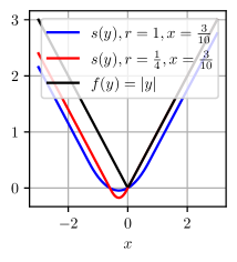
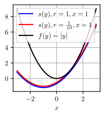
Figure 6.2: The optimistic ellipsoid smoothing. Notice the poor global approximation but good local approximation near $x$.

We want $g$ to be an estimate of $s^{\prime}(x)$, which is

$$s^{\prime}(x) =\frac{1}{\operatorname{vol}(E)}\int_{E}f^{\prime}(\textstyle{\frac{1}{2}}z+\textstyle{\frac{1}{2}}x)\operatorname{d}\!z$$

$$=\frac{1}{\operatorname{vol}(\mathbb{B}^{d}_{1})}\int_{\mathbb{B}^{d}_{1}}f^{\prime}(x+\textstyle{\frac{1}{2}}\Sigma^{1/2}z)\operatorname{d}\!z$$ Change of variables

$$=\frac{2\Sigma^{-1/2}}{\operatorname{vol}(\mathbb{B}^{d}_{1})}\int_{\mathbb{S}^{d-1}_{1}}f(x+\textstyle{\frac{1}{2}}\Sigma^{1/2}\xi)\xi\operatorname{d}\!\xi$$ Stokes’ theorem

$$=\frac{2d\Sigma^{-1/2}}{\operatorname{vol}(\mathbb{S}^{d-1}_{1})}\int_{\mathbb{S}^{d-1}_{1}}f(x+\textstyle{\frac{1}{2}}\Sigma^{1/2}\xi)\xi\operatorname{d}\!\xi$$ Proposition A.1

$$=4d\Sigma^{-1}\mathbb{E}[f(X)(X-x)]\,. X=x+\frac{1}{2}\Sigma^{1/2}\xi$$

Please note we have cheated a little here by assuming that $f$ is differentiable and applying Stokes’ theorem. Fortunately the equality still holds even without differentiability, which is a good exercise. Therefore an unbiased estimator of $s^{\prime}(x)$ is

$$g=4d\Sigma^{-1}Y(X-x)\,.$$

The above considerations yield the following lemma:

Lemma 6.4.

$\mathbb{E}[g]=s^{\prime}(x)$.

The next lemma explores the properties of $s$.

Lemma 6.5.

The following hold:

1. $s$ is convex; and

2. $s(y)\leq f(y)$ for all $y\in K$.

3. If $r\in(0,1)$ and $\Sigma=r^{2}R^{\prime\prime}(x)^{-1}$, then $\mathbb{E}\left[f(X)-s(x)\right]\leq\frac{r}{1-r}$.

4. If $f$ is $\beta$-smooth, then $\mathbb{E}\left[f(X)-s(x)\right]\leq\frac{\beta\operatorname{tr}(\Sigma)}{d}$.

5. If $f$ is $\alpha$-strongly convex, then $s$ is $\frac{\alpha}{2}$-strongly convex.

Proof.

Part (a) follows immediately from convexity of $f$, noting that the second (negated) term in the definition of $s$ is constant as a function of $y$. Part (b) follows from convexity of $f$ as well:

$$s(y) =\frac{1}{\operatorname{vol}(E)}\int_{E}\left(2f\left(\textstyle{\frac{1}{2}}z+\textstyle{\frac{1}{2}}y\right)-f\left(z\right)\right)\operatorname{d}\!z\geq\frac{1}{\operatorname{vol}(E)}\int_{E}f(z)=f(z)\,.$$

For part (b), let $\mathbb{R}\ni u\mapsto h_{\xi}(u)=f(x+u\Sigma^{1/2}\xi)$. By definition $\Sigma=r^{2}R^{\prime\prime}(x)^{-1}$ so that for $u\in[-1/r,1/r]$, $x+u\Sigma^{1/2}\xi\in E^{x}_{1}\subset K$. Therefore $h$ is defined on $[-1/r,1/r]$. Hence, by Proposition 3.5 and the assumption that $f\in\mathscr{F}_{\tiny{\texttt{b}}}$ it follows that $h_{\xi}(u)-h_{\xi}(v)\leq\frac{r|u-v|}{1-r}$ for all $u,v\in[-1,1]$. Therefore, letting $v$ be uniformly distribution on $\mathbb{B}^{d}_{1}$,

$$\mathbb{E}\left[f(X)-s(x)\right] =\mathbb{E}\left[h_{\xi}(1/2)+h_{\xi}(\left\|v\right\|)-2h_{\xi}(\left\|v\right\|/2)\right]$$

$$\leq\frac{r}{1-r}\mathbb{E}\left[\left|\frac{1}{2}-\frac{\left\|v\right\|}{2}\right|+\left|\left\|v\right\|-\frac{\left\|v\right\|}{2}\right|\right]$$

$$\leq\frac{r}{1-r}\,.$$

For part (d),

$$\mathbb{E}\left[f(X)-s(x)\right] =\mathbb{E}\left[h_{\xi}(1/2)+h_{\xi}(\left\|v\right\|)-2h_{\xi}(\left\|v\right\|/2)\right]$$

$$\leq 2\mathbb{E}\left[h_{\xi}(1)-h_{\xi}(0)\right]$$

$$=2\mathbb{E}\left[f(x+\Sigma^{1/2}\xi)-f(x)\right]$$

$$\leq\beta\mathbb{E}\left[\left\|\Sigma^{1/2}\xi\right\|^{2}\right]$$

$$=\frac{\beta\operatorname{tr}(\Sigma)}{d}\,.$$

where in the first inequality we used convexity of $h_{\xi}$ and the second we used Lemma 3.3. Part (e) is left as a straightforward exercise. ∎

6.4  Algorithms and regret analysis

We start by studying an algorithm that relies on neither smoothness nor strong convexity.

⬇

1args: learning rate $\eta>0$, $r\in(0,1)$

2for $t=1$ to $n$

3 compute $x_{t}=\operatornamewithlimits{arg\,min}_{x\in K}\sum_{u=1}^{t-1}\eta\left\langle g_{u},x\right\rangle+R(x)$

4 sample $\xi_{t}$ uniformly from $\mathbb{S}^{d-1}_{1}$

5 play $X_{t}=x_{t}+\frac{r}{2}R^{\prime\prime}(x_{t})^{-1/2}\xi_{t}$ and observe $Y_{t}$

6 compute gradient $g_{t}=\frac{4dY_{t}R^{\prime\prime}(x_{t})(X_{t}-x_{t})}{r^{2}}$

Algorithm 9 Follow the regularised leader with ellipsoidal smoothing

The machinery developed in Section 6.3 combined with Theorem 6.3 leads to a straightforward analysis of Algorithm 9.

Theorem 6.6.

Suppose the losses are in $\mathscr{F}_{\tiny{\texttt{b}}}$ and there is no noise and

$$\eta =2^{-\frac{1}{2}}(\vartheta\log(n))^{\frac{3}{4}}d^{-\frac{1}{2}}n^{-\frac{3}{4}} r =\min\left(1,\,2^{\frac{1}{2}}d^{\frac{1}{2}}n^{-\frac{1}{4}}(\vartheta\log(n))^{\frac{1}{4}}\right)\,.$$

The expected regret of Algorithm 9 is upper bounded by

$$\mathbb{E}[\textrm{Reg}_{n}]\leq 1+4\sqrt{2}(\vartheta\log(n))^{\frac{1}{4}}d^{\frac{1}{2}}n^{\frac{3}{4}}$$

Proof.

By definition, $\left\|X_{t}-x_{t}\right\|_{x_{t}}=\frac{r}{2}\leq\frac{1}{2}$ and therefore $X_{t}\in E^{x_{t}}_{1}\subset K$ where the inclusion follows from Lemma 6.1(a). Hence, the algorithm always plays inside $K$. Using the fact that the losses are in $\mathscr{F}_{\tiny{\texttt{b}}}$ it holds automatically that $\textrm{Reg}_{n}\leq n$ and when $r>\frac{1}{2}$ this already implies the bound in the theorem. Suppose for the remainder that $r\leq\frac{1}{2}$. Similarly, for the same reason we may suppose for the remainder that $n\geq 4\vartheta\log(n)$. Let

$$K_{1/n}=\{x\in K:\pi^{K}_{x_{1}}(x)\leq 1-1/n\}$$

and $x_{\star}=\operatornamewithlimits{arg\,min}_{x\in K_{1/n}}\sum_{t=1}^{n}f_{t}(x)$ with ties broken arbitrarily. Such a point is guaranteed to exist by Proposition 3.6, which also shows that

$$\mathbb{E}[\textrm{Reg}_{n}] \leq 1+\mathbb{E}[\textrm{Reg}_{n}(x_{\star})]\,.$$

Before using Theorem 6.3 we need to confirm that $\eta\left\|g_{t}\right\|_{x_{t}\star}\leq\frac{1}{2}$.

$$\eta\left\|g_{t}\right\|_{x_{t}\star} =\frac{4\eta d|Y_{t}|}{r^{2}}\left\|R^{\prime\prime}(x_{t})(X_{t}-x_{t})\right\|_{x_{t}\star}=\frac{2\eta d|Y_{t}|}{r}\leq\frac{2\eta d}{r}\leq\frac{1}{2}\,,$$

where in the final inequality we used the assumption that $n\geq 4\vartheta\log(n)$. Let $\Sigma_{t}=r^{2}R^{\prime\prime}(x_{t})^{-1}$ and $E_{t}=\{y:\left\|x_{t}-y\right\|_{\Sigma_{t}^{-1}}\leq 1\}=E^{x_{t}}_{r}$. The surrogate in round $t$ is

$$s_{t}(x)=\frac{1}{\operatorname{vol}(E_{t})}\int_{E_{t}}\left(2f_{t}(\textstyle{\frac{1}{2}}y+\textstyle{\frac{1}{2}}x)-f_{t}(y)\right)\operatorname{d}\!y\,.$$

Hence, by Theorem 6.3 and the results in Section 6.3,

$$\mathbb{E}[\textrm{Reg}_{n}] \leq 1+\mathbb{E}\left[\sum_{t=1}^{n}f_{t}(X_{t})-f_{t}(x_{\star})\right]$$

$$\leq 1+\frac{nr}{1-r}+\mathbb{E}\left[\sum_{t=1}^{n}s_{t}(x_{t})-s_{t}(x_{\star})\right]$$ Lemma 6.5(b)(c)

$$\leq 1+\frac{nr}{1-r}+\mathbb{E}\left[\sum_{t=1}^{n}\left\langle s^{\prime}_{t}(x_{t}),x_{t}-x_{\star}\right\rangle\right]$$ Lemma 6.5(a)

$$\leq 1+\frac{nr}{1-r}+\mathbb{E}\left[\sum_{t=1}^{n}\left\langle g_{t},x_{t}-x_{\star}\right\rangle\right]$$ Lemma 6.4

$$\leq 1+\frac{nr}{1-r}+\frac{\vartheta\log(n)}{\eta}+\mathbb{E}\left[\sum_{t=1}^{n}\eta\left\|g_{t}\right\|^{2}_{t\star}\right]$$ Theorem 6.3

$$\leq 1+2nr+\frac{\vartheta\log(n)}{\eta}+\frac{4\eta nd^{2}}{r^{2}}\,,$$

where the final inequality follows since $r\leq 1/2$ and $Y_{t}\in[0,1]$ and

$$\eta\left\|g_{t}\right\|^{2}_{t\star} =\eta\left\|\frac{4dY_{t}R^{\prime\prime}(x_{t})(X_{t}-x_{t})}{r^{2}}\right\|^{2}_{x_{t}\star}\leq\frac{16\eta d^{2}}{r^{4}}\left\|X_{t}-x_{t}\right\|_{R^{\prime\prime}(x_{t})}=\frac{4\eta d^{2}}{r^{2}}\,.$$

The result follows by substituting the values of the constants. ∎

Notice how the dependence on the diameter that appeared in Theorem 5.2 has been replaced with a dependence on the self-concordance parameter $\vartheta$ and logarithmic dependence on the horizon. This can be a significant improvement. For example, when $K$ is a ball, then the bound in Theorem 5.2 depends linearly on $\sqrt{\operatorname{diam}(K)}$ while with a suitable self-concordant barrier the regret in Theorem 6.6 replaces this with $\sqrt{\log(n)}$. Essentially what is happening is that Algorithm 9 moves faster deep in the interior where the losses are necessarily more Lipschitz while Algorithm 7 does not adapt the amount of regularisation to the location of $x_{t}$. For smooth functions the rate can be improved by using Lemma 6.5(d) instead of Lemma 6.5(c).

Theorem 6.7.

Suppose the losses are in $\mathscr{F}_{\tiny{\texttt{b}},\tiny{\texttt{sm}}}$ and there is no noise and

$$r^{2} =\min\left(4,\,2^{\frac{2}{3}}d^{\frac{2}{3}}(\nu\log(n))^{\frac{1}{3}}\beta^{-\frac{1}{3}}\operatorname{diam}(K)^{-\frac{4}{3}}n^{-\frac{1}{3}}\right) \eta =\frac{r}{d}\sqrt{\frac{\vartheta\log(n)}{2n}}\,.$$

Then the expected regret of Algorithm 9 is upper bounded by

$$\mathbb{E}[\textrm{Reg}_{n}]\leq 1+\frac{5d}{4}\sqrt{2\vartheta n\log(n)}+3\cdot 2^{\frac{2}{3}}(\vartheta\beta\operatorname{diam}(K)^{2}\log(n))^{\frac{1}{3}}d^{\frac{2}{3}}n^{\frac{2}{3}}\,.$$

Proof.

Note the condition that $r^{2}\leq 4$ is needed to ensure that $X_{t}\in K$. Repeat the argument in the proof of Theorem 6.6 but replace Lemma 6.5(c) with Lemma 6.5(d), which yields

$$\mathbb{E}[\textrm{Reg}_{n}] \leq 1+\frac{\vartheta\log(n)}{\eta}+\frac{2\eta nd^{2}}{r^{2}}+\frac{\beta}{2d}\sum_{t=1}^{n}\operatorname{tr}(\Sigma_{t})$$

$$\leq 1+\frac{\vartheta\log(n)}{\eta}+\frac{2\eta nd^{2}}{r^{2}}+\frac{\beta nr^{2}\operatorname{diam}(K)^{2}}{2}$$

where in the second inequality we used Lemma 6.1(c) and the definition $\Sigma_{t}=r^{2}R^{\prime\prime}(x_{t})^{-1}$. The result follows by substituting the constants. ∎

The diameter now appears in the bound, as it must. Otherwise you could scale the coordinates and make the regret vanish (Section 3.3). There is no hope to remove the $\sqrt{n}$ term from Theorem 6.7, since even with $\beta=0$ the lower bound for linear bandits says the regret should be at least $\Omega(d\sqrt{n})$.

6.5  Smoothness and strong convexity

We conclude the main body of this chapter by showing that a version of follow the regularised leader can achieve $O(\sqrt{n})$ regret for smooth and strongly convex loss functions. The main modification of the algorithm is that the linear surrogate loss functions are replaced by quadratics. Before that though we need to generalise Theorem 6.3.

Theorem 6.8.

Suppose that $(\hat{f}_{t})_{t=1}^{n}$ is a sequence of self-concordant functions from $K$ to $\mathbb{R}$ and let

$$x_{t}=\operatornamewithlimits{arg\,min}_{x\in K}\underbracket{R(x)+\eta\sum_{u=1}^{t-1}\hat{f}_{u}(x)}_{\Phi_{t-1}(x)}\quad\text{ and }\quad\left\|\cdot\right\|_{t\star}=\left\|\cdot\right\|_{\Phi_{t}^{\prime\prime}(x_{t})^{-1}}\,.$$

Then, provided that $\eta\|\hat{f}^{\prime}_{t}(x_{t})\|_{t\star}\leq\frac{1}{2}$ for all $t$, for any $x\in\operatorname{int}(K)$,

$$\widehat{\textrm{Reg}}_{n}(x)=\sum_{t=1}^{n}\left(\hat{f}_{t}(x_{t})-\hat{f}_{t}(x)\right)\leq-\frac{\vartheta}{\eta}\log\left(1-\pi^{K}_{x_{1}}(x)\right)+\eta\sum_{t=1}^{n}\|\hat{f}_{t}^{\prime}(x_{t})\|^{2}_{t\star}\,,$$

Theorem 6.3 is recovered by choosing $\hat{f}_{t}(x)=\left\langle g_{t},x\right\rangle$.

Proof.

By the definition of $\Phi_{t}$,

$$\widehat{\textrm{Reg}}_{n}(x)=\sum_{t=1}^{n}\left(\hat{f}_{t}(x_{t})-\hat{f}_{t}(x)\right)$$

$$=\frac{1}{\eta}\sum_{t=1}^{n}\left(\Phi_{t}(x_{t})-\Phi_{t-1}(x_{t})\right)-\frac{\Phi_{n}(x)}{\eta}+\frac{R(x)}{\eta}$$

$$=\frac{1}{\eta}\sum_{t=1}^{n}\left(\Phi_{t}(x_{t})-\Phi_{t}(x_{t+1})\right)+\frac{\Phi_{n}(x_{n+1})}{\eta}-\frac{\Phi_{n}(x)}{\eta}+\frac{R(x)-R(x_{1})}{\eta}$$

$$\leq\frac{1}{\eta}\sum_{t=1}^{n}\left(\Phi_{t}(x_{t})-\Phi_{t}(x_{t+1})\right)+\frac{R(x)-R(x_{1})}{\eta} \Phi_{n}(x_{n+1})\leq\Phi_{n}(x)$$

$$\leq\eta\sum_{t=1}^{n}\|\hat{f}^{\prime}_{t}(x_{t})\|^{2}_{t\star}+\frac{R(x)-R(x_{1})}{\eta}$$ Lemma 6.2

$$\leq-\frac{\vartheta}{\eta}\log\left(1-\pi_{x_{1}}^{K}(x)\right)+\eta\sum_{t=1}^{n}\|\hat{f}_{t}(x_{t})\|^{2}_{t\star}\,.$$ Lemma 6.1(d)

Note that in the application of Lemma 6.2 we used the fact that $\hat{f}_{t}^{\prime}(x_{t})=\Phi^{\prime}_{t}(x_{t})$ and the assumption that $\eta\|\hat{f}_{t}^{\prime}(x_{t})\|_{t\star}\leq\frac{1}{2}$. ∎

⬇

1args: learning rate $\eta>0$

2for $t=1$ to $n$

3 let $x_{t}=\operatornamewithlimits{arg\,min}_{x\in K}\left[R(x)+\eta\sum_{u=1}^{t-1}\left(\left\langle g_{u},x\right\rangle+\frac{\alpha}{4}\left\|x-x_{u}\right\|^{2}\right)\right]$

4 let $\Sigma_{t}^{-1}=R^{\prime\prime}(x_{t})+\frac{\eta\alpha t}{4}\mathds{1}$

5 sample $\xi_{t}$ uniformly from $\mathbb{S}^{d-1}_{1}$

6 play $X_{t}=x_{t}+\frac{1}{2}\Sigma_{t}^{1/2}\xi_{t}$ and observe $Y_{t}$

7 compute gradient $g_{t}=4dY_{t}\Sigma_{t}^{-1}(X_{t}-x_{t})$

Algorithm 10 Follow the regularised leader with ellipsoidal smoothing

Theorem 6.9.

Suppose the losses are in $\mathscr{F}_{\tiny{\texttt{b}},\tiny{\texttt{sm}},\tiny{\texttt{sc}}}$ and there is no noise and

$$\eta=\frac{2}{d}\sqrt{\frac{\left(\vartheta+\frac{\beta}{\alpha}\right)[1+\log(n)]}{n}}\,.$$

Then the expected regret of Algorithm 10 is upper bounded by

$$\mathbb{E}[\textrm{Reg}_{n}]\leq 1+4d\sqrt{n\left(\vartheta+\frac{4\beta}{\alpha}\right)[1+\log(n)]}\,.$$

Proof.

The same argument in the proof of Theorem 6.6 shows that $X_{t}$ is in the Dikin ellipsoid associated with $R$ at $x_{t}$ and therefore is in $K$. Let

$$K_{1/n}=\{x\in K:\pi^{K}_{x_{1}}(x)\leq 1-1/n\}$$

and $x_{\star}=\operatornamewithlimits{arg\,min}_{x\in K_{1/n}}\sum_{t=1}^{n}f_{t}(x)$, which by Proposition 3.6 and Lemma 6.5(b)(d) means that

$$\mathbb{E}[\textrm{Reg}_{n}] \leq 1+\mathbb{E}[\textrm{Reg}_{n}(x_{\star})]$$

$$=1+\mathbb{E}\left[\sum_{t=1}^{n}(f_{t}(X_{t})-f_{t}(x_{\star}))\right]$$

$$\leq 1+\mathbb{E}\left[\sum_{t=1}^{n}\left(s_{t}(x_{t})-s_{t}(x_{\star})+\frac{\beta}{d}\operatorname{tr}(\Sigma_{t})\right)\right]\,.$$

Next, let $\hat{f}_{t}(x)=\left\langle g_{t},x-x_{t}\right\rangle+\frac{\alpha}{4}\left\|x-x_{t}\right\|^{2}$. By Lemma6.5(e), $s_{t}$ is $\frac{\alpha}{2}$-strongly convex and therefore

$$\mathbb{E}\left[\sum_{t=1}^{n}(s_{t}(x_{t})-s_{t}(x_{\star}))\right] \leq\mathbb{E}\left[\sum_{t=1}^{n}\left(\left\langle\mathbb{E}_{t-1}[g_{t}],x_{t}-x_{\star}\right\rangle-\frac{\alpha}{4}\left\|x_{t}-x_{\star}\right\|^{2}\right)\right]$$

$$=\mathbb{E}\left[\sum_{t=1}^{n}(\hat{f}_{t}(x_{t})-\hat{f}_{t}(x_{\star}))\right]$$

$$\leq\frac{\vartheta\log(n)}{\eta}+\eta\mathbb{E}\left[\sum_{t=1}^{n}\left\|g_{t}\right\|^{2}_{\Sigma_{t}}\right]$$ Theorem 6.8

$$\leq\frac{\vartheta\log(n)}{\eta}+4\eta nd^{2}\,.$$

Using the definition of $\Sigma_{t}$,

$$\frac{\beta}{d}\sum_{t=1}^{n}\operatorname{tr}(\Sigma_{t}) \leq\frac{4\beta}{\alpha\eta}\sum_{t=1}^{n}\frac{1}{t}\leq\frac{4\beta}{\alpha\eta}(1+\log(n))\,.$$

Combining everything shows that

$$\mathbb{E}[\textrm{Reg}_{n}] \leq 1+4\eta nd^{2}+\frac{1}{\eta}\left(\vartheta\log(n)+\frac{4\beta}{\alpha}(1+\log(n))\right)\,.$$

The result follows by substituting the definition of $\eta$. ∎

6.6  Notes

1. At no point in this chapter did we need Lipschitz losses. The analysis essentially exploits the fact that convex functions cannot have large gradients except very close to the boundary where the regularisation provided by the self-concordant barrier prevents the blowup in variance from severely impacting the regret.

2. We have made several improvements to the statistical efficiency relative to the algorithm presented in Chapter 5. In exchange the algorithms are more complicated and computationally less efficient. Algorithms based on gradient descent run in $O(d)$ time per round except those rounds where a projection is needed. Furthermore, even when the projection is needed it is with respect to the euclidean norm and likely to be extremely fast. Meanwhile the algorithms in this chapter need a singular value decomposition to compute $X_{t}$, solve an optimisation problem to find $x_{t}$ and need oracle access to a $\vartheta$-self-concordant barrier.

3. The reader interested in knowing more about ($\vartheta$-)self-concordant barriers is referred to the wonderful notes by Nemirovski (1996). The most obvious question is whether or not these things even exist. We give some examples:

   • When $K=\{x:\left\langle a_{i},x\right\rangle\leq b_{i},1\leq i\leq k\}$ is a polytope defined by $k$ half-spaces, then $R(x)=-\sum_{i=1}^{k}\log(b_{i}-\left\langle a_{i},x\right\rangle)$ is called the logarithmic barrier and is $k$-self-concordant.

   • When $K=\{x:\left\|x\right\|\leq\rho\}$ is a ball, then $R(x)=-\log(\rho^{2}-\left\|x\right\|^{2})$ is a $1$-self-concordant barrier on $K$.

   • For any convex body $K$ there exists a $\vartheta$-self-concordant barrier with $\vartheta\leq d$. Specifically, the entropic barrier satisfies this (Chewi, 2023; Bubeck and Eldan, 2014).

4. As far as we know Algorithm 9 has not been analysed previously. Algorithm 10 and Theorem 6.9 is due to Hazan and Levy (2014) while Theorem 6.7 is by Saha and Tewari (2011).

5. The surrogate loss only appears in the analysis. Interestingly, Hazan and Levy (2014) and Saha and Tewari (2011) analysed their algorithms using the surrogate

   $$s_{t}(y)=\frac{1}{\operatorname{vol}(E^{x_{t}}_{r})}\int_{E^{x_{t}}_{r}-x_{t}}f(y+u)\operatorname{d}\!u\,,$$

   which is the ellipsoidal analogue of the surrogate used in Chapter 5. Except for a constant factor this surrogate has the same gradient at $x_{t}$ as the surrogate we used, which means the resulting algorithms are the same. The difficulty is that the surrogate defined above is not defined on all of $K$, which forces various contortions or assumptions in the analysis.

6. Note that Theorem 6.6 and 6.7 bound the regret for the same algorithm with different learning rates and smoothing parameters. You should wonder if it is possible to obtain the best of both bounds with a single algorithm by adaptively tuning the learning rates. At present this is not known as far as we know.

Chapter 7  Linear and quadratic bandits

Function classes like $\mathscr{F}_{\tiny{\texttt{b}}}$ are non-parametric. In this chapter we shift gears a little by studying two important parametric classes: $\mathscr{F}_{\tiny{\texttt{b}},\tiny{\texttt{lin}}}$ and $\mathscr{F}_{\tiny{\texttt{b}},\tiny{\texttt{quad}}}$. The main purpose of this chapter is to explain the differences between convex bandits and linear bandits and to prove a minimax bound on the regret for quadratic bandits. The latter is not established for a polynomial time algorithm but serves as a target in future chapters. Before the algorithms and regret analysis we need two tools.

7.1  Covering numbers

Given $A,B\subset\mathbb{R}^{d}$, the covering number

$$N(A,B)=\min\left\{|\mathcal{C}|:\mathcal{C}\subset\mathbb{R}^{d},A\subset\bigcup_{x\in\mathcal{C}}(x+B)\right\}$$

is the smallest number of translates of $B$ needed to cover $A$.

Proposition 7.1 (Artstein-Avidan et al. 2015, Corollary 4.1.15).

Suppose that $A$ is centrally symmetric, compact and convex. Then, for any $\varepsilon\in(0,1)$,

$$N(A,\varepsilon A)\leq\left(1+\frac{2}{\varepsilon}\right)^{d}\,.$$

Proposition 7.2.

Suppose that $A$ is compact and centrally symmetric. Then, for any $\varepsilon\in(0,1)$,

$$N(A,\varepsilon\operatorname{conv}(A))\leq\left(1+\frac{4}{\varepsilon}\right)^{d}\,.$$

Proof.

Let $B=\operatorname{conv}(A)$ and take a cover $\mathcal{C}$ so that $B\subset\bigcup_{x\in\mathcal{C}}(x+\frac{\varepsilon}{2}B)$ and then project points in $\mathcal{C}$ onto $A$ using $\left\|\cdot\right\|_{B}$, which is the norm such that $B=\{x\in\mathbb{R}^{d}:\left\|x\right\|_{B}\leq 1\}$. ∎

7.2  Optimal design

An optimal design for a compact set $A\subset\mathbb{R}^{d}$ is a probability measure on $\mathbb{R}^{d}$ that minimises the worst case variance of a least-squares estimator over $A$. The following theorem gives the definition and establishes existence.

Theorem 7.3 (Kiefer and Wolfowitz 1960).

For any compact $A$ subset $\mathbb{R}^{d}$ with $\operatorname{span}(A)=\mathbb{R}^{d}$ there exists a probability measure $\pi$ supported on $A$ such that

$$\left\|x\right\|^{2}_{G_{\pi}^{-1}}=d\text{ for all }x\in A\,,$$

where $G_{\pi}=\int_{A}xx^{\top}\operatorname{d}\!\pi(x)$

Remarkably the constant $d$ is the best achievable for any compact $A$ with $\operatorname{span}(A)=\mathbb{R}^{d}$ in the sense that:

$$\min_{\pi\in\Delta_{A}}\max_{x\in A}\left\|x\right\|^{2}_{G_{\pi}^{-1}}=d\,.$$

7.3  Exponential weights

Let $\mathcal{C}$ be a finite set and $\ell_{1},\ldots,\ell_{n}$ a sequence of functions from $\mathcal{C}\to\mathbb{R}$. Given a learning rate $\eta$ define a distribution $q_{t}$ on $\mathcal{C}$ by

$$q_{t}(a)=\frac{\exp\left(-\eta\sum_{u=1}^{t-1}\ell_{u}(a)\right)}{\sum_{b\in\mathcal{C}}\exp\left(-\eta\sum_{u=1}^{t-1}\ell_{u}(b)\right)}\,.$$

Theorem 7.4.

Suppose that $\eta|\ell_{t}(a)|\leq 1$ for all $1\leq t\leq n$, then

$$\max_{b\in\mathcal{C}}\sum_{t=1}^{n}\left(\sum_{a\in\mathcal{C}}q_{t}(a)\ell_{t}(a)-\ell_{t}(b)\right)\leq\frac{\log|\mathcal{C}|}{\eta}+\frac{\eta}{2}\sum_{t=1}^{n}\sum_{a\in\mathcal{C}}q_{t}(a)\ell_{t}(a)^{2}\,.$$

Proof.

We use the following two inequalities:

1. $\exp(x)\leq 1+x+x^{2}$ for all $|x|\leq 1$; and

2. $\log(1+x)\leq x$ for all $x>0$.

Let $b=\operatornamewithlimits{arg\,min}_{a\in\mathcal{C}}\sum_{t=1}^{n}\ell_{t}(a)$ and $D_{t}=\log(1/q_{t}(b))$. Then,

$$D_{t+1} =\log\left(\frac{1}{q_{t+1}(b)}\right)$$

$$=\log\left(\frac{\sum_{a\in\mathcal{C}}q_{t}(a)\exp\left(-\eta\ell_{t}(a)\right)}{q_{t}(b)\exp\left(-\eta\ell_{t}(b)\right)}\right)$$

$$=D_{t}+\log\left(\sum_{a\in\mathcal{C}}q_{t}(a)\exp\left(-\eta\ell_{t}(a)\right)\right)-\eta\ell_{t}(b)$$

$$\leq D_{t}+\log\left(\sum_{a\in\mathcal{C}}q_{t}(a)\left[1-\eta\ell_{t}(a)+\eta^{2}\ell_{t}(a)^{2}\right]\right)-\eta\ell_{t}(b)$$ by (a)

$$=D_{t}+\log\left(1+\sum_{a\in\mathcal{C}}q_{t}(a)\left[-\eta\ell_{t}(a)+\eta^{2}\ell_{t}(a)^{2}\right]\right)-\eta\ell_{t}(b)$$

$$\leq D_{t}-\eta\sum_{a\in\mathcal{C}}\left[q_{t}(a)\ell_{t}(a)-\ell_{t}(b)\right]+\eta^{2}\sum_{a\in\mathcal{C}}q_{t}(a)\ell_{t}(a)^{2}\,.$$ by (b)

Rearranging and summing over $t$ and telescoping yields

$$\sum_{t=1}^{n}\left(\sum_{a\in\mathcal{C}}q_{t}(a)\ell_{t}(a)-\ell_{t}(b)\right) \leq\frac{1}{\eta}\log\left(\frac{q_{n+1}(b)}{q_{1}(b)}\right)+\eta\sum_{t=1}^{n}\sum_{a\in\mathcal{C}}q_{t}(a)\ell_{t}(a)^{2}$$

$$\leq\frac{1}{\eta}\log\left(|\mathcal{C}|\right)+\eta\sum_{t=1}^{n}\sum_{a\in\mathcal{C}}q_{t}(a)\ell_{t}(a)^{2}\,.\qed$$

7.4  Linear bandits

For this section we make the following assumption:

1. $(f_{t})_{t=1}^{n}$ are in $\mathscr{F}_{\tiny{\texttt{b}},\tiny{\texttt{lin}}}$.

2. $K\subset\mathbb{R}^{d}$ is compact but not necessarily convex.

3. $\operatorname{span}(K)=\mathbb{R}^{d}$.

We let $(\theta_{t})_{t=1}^{n}$ be a sequence in $\mathbb{R}^{d}$ such that $f_{t}(x)=\left\langle x,\theta_{t}\right\rangle$. The plan is to use exponential weights on a finite $\mathcal{C}\subset K$ that is sufficiently large that the optimal action in $K$ can be approximated by something in $\mathcal{C}$. Let $A=\operatorname{conv}(K-K)$, which is a symmetric convex set. By the assumption that the losses are bounded,

$$\theta_{t}\in\Theta=\left\{\theta\in\mathbb{R}^{d}:\left\|\theta\right\|_{A^{\circ}}\leq 1\right\}\,.$$

What we need from $\mathcal{C}$ is that for all $\theta\in\Theta$,

$$\min_{x\in\mathcal{C}}\max_{y\in K}\left\langle x-y,\theta\right\rangle\leq\varepsilon\,.$$

Suppose that $\left\|x-y\right\|_{A}\leq\varepsilon$, then $\left\langle x-y,\theta\right\rangle\leq\left\|x-y\right\|_{A}\left\|\theta\right\|_{A^{\circ}}\leq\varepsilon$. Hence, it suffices to choose $\mathcal{C}\subset K$ such that $K\subset\bigcup_{x\in\mathcal{C}}(x+\varepsilon A)$. By Proposition 7.2, such a cover exists with

$$|\mathcal{C}|\leq\left(1+\frac{4}{\varepsilon}\right)^{d}\,.$$

The algorithm for linear bandits plays actions in $\mathcal{C}$ and uses importance-weighted least squares to estimate $\left\langle x,\theta_{t}\right\rangle$ for all $x\in\mathcal{C}$ simultaneously. The distribution proposed by exponential weights is mixed with a small amount of an optimal design on $\mathcal{C}$, which is needed so that the estimates are suitably bounded as required by Theorem 8.1.

⬇

1args: $\eta>0$, $\gamma>0$, $K$

2find $\mathcal{C}\subset K$ such that $\min_{x\in\mathcal{C}}\max_{y\in K}\left\|x-y\right\|_{A}\leq\frac{1}{n}$

3find optimal design $\pi$ on $\mathcal{C}$

4for $t=1$ to $n$

5 let $q_{t}(x)=\frac{\exp\left(-\eta\sum_{u=1}^{t-1}\langle x,\hat{\theta}_{u}\rangle\right)}{\sum_{y\in\mathcal{C}}\exp\left(-\eta\sum_{u=1}^{t-1}\langle y,\hat{\theta}_{u}\rangle\right)}$

6 let $p_{t}=(1-\gamma)q_{t}+\gamma\pi$

7 sample $X_{t}$ from $p_{t}$ and observe $Y_{t}=f_{t}(X_{t})$

8 let $G_{t}=\sum_{a\in\mathcal{C}}p_{t}(a)aa^{\top}$ and $\hat{\theta}_{t}=G_{t}^{-1}X_{t}Y_{t}$

Algorithm 11 Exponential weights for linear bandits

Theorem 7.5.

Suppose that

$$\eta =\frac{1}{2}\sqrt{\frac{\log|\mathcal{C}|}{nd}} \gamma =\eta d\,.$$

Then the regret of Algorithm 11 is bounded by

$$\mathbb{E}[\textrm{Reg}_{n}]\leq 1+4\sqrt{nd\log|\mathcal{C}|}\,.$$

Proof.

Recall the definition of $G_{\pi}$ from Section 7.2 and let

$$G_{q_{t}}=\sum_{x\in\mathcal{C}}q_{t}(x)xx^{\top}\,.$$

With this notation, $G_{t}=(1-\gamma)G_{q_{t}}+\gamma G_{\pi}$. Since the exponential weights distribution is supported on all $x\in K$ and $\operatorname{span}(K)=\mathbb{R}^{d}$, $G_{t}$ is invertible. Next,

$$\mathbb{E}_{t-1}[\hat{\theta}_{t}] =\sum_{x\in\mathcal{C}}p_{t}(x)G_{t}^{-1}x\left\langle x,\theta_{t}\right\rangle=\theta_{t}\,.$$

Furthermore,

$$\mathbb{E}_{t-1}\big{[}\langle x,\hat{\theta}_{t}\rangle^{2}\big{]} =\mathbb{E}_{t-1}\big{[}Y_{t}^{2}x^{\top}G_{t}^{-1}X_{t}X_{t}^{\top}G_{t}^{-1}x\big{]}\leq\left\|x\right\|^{2}_{G_{t}^{-1}}\,,$$

where we used the fact that $Y_{t}^{2}\leq 1$. Therefore,

$$\mathbb{E}_{t-1}\left[\sum_{x\in\mathcal{C}}q_{t}(x)\langle x,\hat{\theta}_{t}\rangle^{2}\right] \leq\sum_{x\in\mathcal{C}}q_{t}(x)\left\|x\right\|^{2}_{G_{t}^{-1}}$$

$$\leq\frac{1}{1-\gamma}\sum_{x\in\mathcal{C}}q_{t}(x)\left\|x\right\|^{2}_{G_{q_{t}}^{-1}}$$

$$=\frac{d}{1-\gamma}\,.$$

We also need to show the loss estimates are suitably bounded:

$$\eta|\langle x,\hat{\theta}_{t}\rangle| =\eta\left|x^{\top}G_{t}^{-1}X_{t}Y_{t}\right|\leq\eta\left\|x\right\|_{G_{t}^{-1}}\left\|X_{t}\right\|_{G_{t}^{-1}}\leq\frac{\eta d}{\gamma}=1\,.$$

Define $x_{\star}=\operatornamewithlimits{arg\,min}_{x\in\mathcal{C}}\sum_{t=1}^{n}\left\langle x_{\star},\theta_{t}\right\rangle$. Then, the regret is bounded by

$$\mathbb{E}[\textrm{Reg}_{n}] =1+\mathbb{E}\left[\sum_{t=1}^{n}\langle X_{t}-x_{\star},\theta_{t}\rangle\right]$$

$$=1+\mathbb{E}\left[\sum_{t=1}^{n}\sum_{x\in\mathcal{C}}p_{t}(x)\langle x-x_{\star},\theta_{t}\rangle\right]$$

$$\leq 1+n\gamma+\mathbb{E}\left[\sum_{t=1}^{n}\sum_{x\in\mathcal{C}}q_{t}(x)\langle x-x_{\star},\theta_{t}\rangle\right]$$

$$=1+n\gamma+\mathbb{E}\left[\sum_{t=1}^{n}\sum_{x\in\mathcal{C}}q_{t}(x)s\left\langle x-x_{\star},\hat{\theta}_{t}\right\rangle\right]$$

$$\leq 1+n\gamma+\frac{\log|\mathcal{C}|}{\eta}+\mathbb{E}\left[\sum_{t=1}^{n}\sum_{x\in\mathcal{C}}q_{t}(x)\langle x,\hat{\theta}_{t}\rangle^{2}\right]$$

$$\leq 1+n\gamma+\frac{\log|\mathcal{C}|}{\eta}+\frac{\eta nd}{1-\gamma}\,.$$

The result follows by substituting the constants. ∎

7.5  Quadratic bandits

Quadratic bandits seem much harder than linear bandits but if you ignore the computation complexity then it turns out that quadratic bandits are linear bandits. Define a function $\phi(x):\mathbb{R}^{d}\to\mathbb{R}^{d(d+3)/2}$ by

$$\phi(x)=(x_{1},\ldots,x_{d},x_{1}^{2},x_{1}x_{2},\ldots,x_{1}x_{d},x_{2}^{2},x_{2}x_{3},\ldots,x_{d-1}^{2},x_{d-1}x_{d},x_{d}^{2})\,.$$

So $\phi$ is the feature map associated with the polynomial kernel of degree 2. You should check that any $f\in\mathscr{F}_{\tiny{\texttt{b}},\tiny{\texttt{quad}}}$ can be written as $f(x)=\left\langle\phi(x),\theta\right\rangle$ for some $\theta\in\mathbb{R}^{d(d+3)/2}$.

Lemma 7.6.

Given $K\subset\mathbb{R}^{d}$, there exists a $\mathcal{C}\subset K$ such that:

1. $\log|\mathcal{C}|\leq d\log\left(\frac{3d(d+3)}{\varepsilon}\right)$.

2. $\max_{x\in K}\min_{y\in\mathcal{C}}\left\|\phi(x)-\phi(y)\right\|_{\operatorname{conv}(\phi(K)-\phi(K))}\leq\varepsilon$.

The proof is left as an exercise. We can now simply write the kernelised version of Algorithm 11.

⬇

1args: $\eta>0$, $\gamma>0$ and $K$

2find $\mathcal{C}\subset K$ satisfying (a),(b) in Lemma 7.6, $\varepsilon=\frac{1}{n}$

3find optimal design $\pi$ on $\{\phi(a):a\in\mathcal{C}\}$

4for $t=1$ to $n$

5 let $q_{t}(x)=\frac{\exp\left(-\eta\sum_{u=1}^{t-1}\left\langle\phi(x),\hat{\theta}_{u}\right\rangle\right)}{\sum_{x\in\mathcal{C}}\exp\left(-\eta\sum_{u=1}^{t-1}\left\langle\phi(x),\hat{\theta}_{u}\right\rangle\right)}$

6 let $p_{t}=(1-\gamma)q_{t}+\gamma\pi$

7 sample $X_{t}$ from $p_{t}$ and observe $Y_{t}=f_{t}(X_{t})$

8 let $G_{t}=\sum_{a\in\mathcal{C}}p_{t}(a)\phi(a)\phi(a)^{\top}$ and $\hat{\theta}_{t}=G_{t}^{-1}X_{t}Y_{t}$

Algorithm 12 Exponential weights for quadratic bandits

An immediate corollary of Theorem 7.5 is the following bound on the regret of Algorithm 12

Theorem 7.7.

With parameters

$$\eta =\frac{1}{2}\sqrt{\frac{\log|\mathcal{C}|}{nd(d+1/3)}} \gamma =nd(d+1)/3$$

The expected regret of Algorithm 12 is bounded by

$$\mathbb{E}[\textrm{Reg}_{n}]\leq 1+4\sqrt{\frac{n(d+1)d^{2}\log(3nd(d+1))}{3}}\,.$$

Ignoring logs and constants, Theorem 7.7 shows that one can obtain $d^{1.5}\sqrt{n}$ regret for quadratic bandits. Note that we did not use anywhere that $\mathscr{F}_{\tiny{\texttt{b}},\tiny{\texttt{quad}}}$ only included convex quadratics. Everything works for more general quadratic losses. Even if we restrict our attention to convex quadratics, none of the algorithms we have presented so far can match this bound. Actually no efficient algorithm is known matching this bound except for special $K$.

7.6  Linear bandits via self-concordance

Before we return to convex bandits, we want to illustrate why gradient-based methods can be near-optimal for linear bandits but are hard to make work for convex bandits. We start by adapting the algorithm in Chapter 6 to the linear setting. For this section we assume that:

1. The losses are in $\mathscr{F}_{\tiny{\texttt{b}},\tiny{\texttt{lin}}}$; and

2. $K$ is a convex body in $\mathbb{R}^{d}$; and

3. $R$ is $\vartheta$-self-concordant barrier on $K$.

The algorithm we study is actually identical to Algorithm 9 except that we set $r=1$, which means the algorithm samples from the boundary of the Dikin ellipsoid rather than a scaled-down Dikin ellipsoid. Note that we could not have chosen $r$ larger because then the algorithm might play outside of the constraint set $K$.

⬇

1initialise $x_{1}=\operatornamewithlimits{arg\,min}_{x\in K}R(x)$

2for $t=1$ to $n$

3 compute $x_{t}=\operatornamewithlimits{arg\,min}_{x\in K}\sum_{u=1}^{t}\eta\left\langle g_{u},x\right\rangle+R(x)$

4 sample $X_{t}$ uniformly from $\{y:\left\|y-x_{t}\right\|_{R^{\prime\prime}(x_{t})}=1\}$

5 compute gradient $g_{t}=dR^{\prime\prime}(x_{t})Y_{t}(X_{t}-x_{t})$

Algorithm 13 SCRiBLe

Theorem 7.8.

Suppose that

$$\eta=\frac{1}{d}\sqrt{\frac{\vartheta\log(n)}{2n}}\,.$$

Then the expected regret of Algorithm 13 is upper bounded by

$$\mathbb{E}[\textrm{Reg}_{n}] \leq 1+d\sqrt{2\vartheta n\log(n)}\,.$$

Proof.

Let $K_{1/n}=\{x\in K:\pi_{x_{1}}(x)\leq 1-1/n\}$ where $x_{1}=\operatornamewithlimits{arg\,min}_{x\in K}R(x)$. Next, let $x_{\star}=\operatornamewithlimits{arg\,min}_{x\in K}\sum_{t=1}^{n}f_{t}(x)$, which by Proposition 3.6,

$$\mathbb{E}[\textrm{Reg}_{n}] =\max_{x\in K}\mathbb{E}\left[\sum_{t=1}^{n}f_{t}(X_{t})-f_{t}(x)\right]$$

$$\leq 1+\mathbb{E}\left[\sum_{t=1}^{n}f_{t}(X_{t})-f_{t}(x_{\star})\right]$$

$$=1+\mathbb{E}\left[\sum_{t=1}^{n}\left\langle x_{t}-x_{\star},\hat{\theta}_{t}\right\rangle\right]$$

$$\leq 1+\frac{\vartheta\log(n)}{\eta}+2\eta\mathbb{E}\left[\sum_{t=1}^{n}\|\hat{\theta}_{t}\|^{2}_{x_{t}\star}\right]\,.$$ Theorem 6.3

The dual norm term is bounded as follows:

$$\mathbb{E}_{t-1}\left[\|\hat{\theta}_{t}\|^{2}_{x_{t}\star}\right] =d^{2}\mathbb{E}_{t-1}\left[Y_{t}^{2}\|X_{t}-x_{t}\|_{R^{\prime\prime}(x_{t})}^{2}\right]$$

$$\leq d^{2}\mathbb{E}_{t-1}\left[\|X_{t}-x_{t}\|_{R^{\prime\prime}(x_{t})}^{2}\right]$$

$$=d^{2}\,.$$

Therefore,

$$\mathbb{E}[\textrm{Reg}_{n}] \leq 1+\frac{\vartheta\log(n)}{\eta}+2n\eta d^{2}\,.$$

The result follows by substituting the definition of $\eta$. ∎

We should compare Theorem 7.5 and Theorem 7.8. size=,color=red!20!white,]Tor: do this

7.7  Notes

1. Our analysis of linear bandits was entirely geared towards applying the naive covering argument to quadratic bandits showing that for this class the regret is at most $d^{1.5}\sqrt{n}$.

2. Even when $K$ is convex, (non-convex) quadratic programming is computationally hard. For example, when $K$ is a simplex and $A$ is the adjacency matrix of an undirected graph $G$, then a theorem by Motzkin and Straus (1965) says that

   $$\frac{1}{2}\min_{x\in\Delta_{d}}(-x^{\top}Ax)=\frac{1}{2}\left(\frac{1}{\omega(G)}-1\right)\,,$$

   where $\omega(G)$ is the size of the largest clique in $G$. Since the clique decision problem is NP-complete (Karp, 1972), there (probably) does not exist an efficient algorithm for minimising quadratic functions over the simplex.

3. By the previous note, Algorithm 12 cannot be implemented efficiently, since its analysis did not make use of convexity of the losses. Sadly, even if we restrict our attention to convex quadratic loss functions and convex $K$, the kernel method does not seem amenable to efficient calculations. Why not? The problem is that even if $K$ is convex, the set $J=\{\phi(a):a\in K\}$ need not be convex.

4. The assumption that $K$ spans $\mathbb{R}^{d}$ in Section 7.4 was for simplicity only. In case this does not hold you can either reparameterise everything via an isometry between $K$ and $\mathbb{R}^{\dim(K)}$ or replace inverses with pseudoinverses in the algorithm and analysis.

5. You can find much more about linear bandits in the book by Lattimore and Szepesvári (2020). Provided that $K$ is given in terms of a separation oracle, there is a polynomial time algorithm for which the expected regret is upper bounded by $d\sqrt{n}$.

6. Algorithm 13 is due to Abernethy et al. (2008) while Algorithm 11 is by Bubeck et al. (2012).

Chapter 8  Continuous exponential weights

Throughout this chapter we will assume that:

1. The losses are in $\mathscr{F}_{\tiny{\texttt{b}}}$.

2. There is no noise so that $Y_{t}=f_{t}(X_{t})$.

The assumption on the noise is for simplicity only. You could have a pleasant afternoon checking that everything goes through with no serious changes in the presence of subgaussian noise.

8.1  Continuous exponential weights

Unlike gradient and second-order methods, continuous exponential weights uses the entire loss function and acts in the space of probability measures on $K$. This introduces an interesting complexity. Rather than estimating a gradient and (maybe) Hessian, the learner now has to estimate the entire loss function from a single query.

⬇

1args: learning rate $\eta>0$

2for $t=1$ to $n$

3 compute density $q_{t}(x)=\frac{\bm{1}_{K}(x)\exp\left(-\eta\sum_{u=1}^{t-1}\hat{f}_{u}(x)\right)}{\int_{K}\exp\left(-\eta\sum_{u=1}^{t-1}\hat{f}_{u}(x)\right)}$

4 find distribution $p_{t}$ supported on $K$

5 sample $X_{t}$ from $p_{t}$ and observe $Y_{t}$

6 compute estimator $\hat{f}_{t}:K\to\mathbb{R}$ using $X_{t},Y_{t},p_{t},q_{t}$

Algorithm 14 Abstract continuous exponential weights

As we have seen in other abstract algorithms, we will insist that the distribution $p_{t}$ is constructed as a function of $q_{t}$ only. You should think of $q_{t}$ as encoding the state of the algorithm. Bayesian’s may like to think of $q_{t}$ as some kind of posterior. Very often in applications of continuous exponential weights $p_{t}$ is chosen to be equal to $q_{t}$. Or sometimes something very close. For example, in linear bandits one commonly takes $p_{t}=(1-\gamma)q_{t}+\gamma p$ where $p$ is an optimal design on $K$ (Lattimore and Szepesvári, 2020, Chapters 21 and 27).

8.2  Convex analysis for continuous exponential weights

Before progressing further we need to introduce some simplifying notation and a few tools from convex analysis. Given $p\in\Delta_{K}$ and $f:K\to\mathbb{R}$ let $\left\langle p,f\right\rangle=\int_{K}p(x)f(x)\operatorname{d}\!x$. The negative entropy function is $R:\mathscr{M}(K)\to\mathbb{R}$ defined by

$$R(p)=\int_{K}\log(p(x))\operatorname{d}\!x-\int_{K}p(x)\operatorname{d}\!x\,,$$

which is a convex function on $\mathscr{M}(K)$. We let $\operatorname{D}$ be the Bregman divergence with respect to $R$, which is given by

$$\operatorname{D}(p,q)=R(p)-R(q)-DR(p)[p-q]\,.$$

You should check that for $p,q\in\mathscr{M}(K)$, $\operatorname{D}(p,q)=\int_{K}p(x)\log(p(x)/q(x))\operatorname{d}\!x$ is the relative entropy. Remember that the Fenchel dual of $R$ is

$$R^{\star}(f)=\sup_{p\in\mathscr{M}(K)}\left\langle p,f\right\rangle-R(p)\,.$$

Lastly, the Bregman divergence with respect to $R^{\star}$ is denoted by

$$\operatorname{D}^{\star}(f,g)=R^{\star}(f)-R^{\star}(g)-DR^{\star}(g)[f-g]\,.$$

Recalling the notation from Algorithm 14 and for $p\in\Delta_{K}$ let

$$\widehat{\textrm{Reg}}_{n}(p)=\sum_{t=1}^{n}\left\langle q_{t}-p,\hat{f}_{t}\right\rangle$$

be the regret of the sequence of distributions $p_{t}$ compared to $p$ on estimated loss functions $(\hat{f}_{t})_{t=1}^{n}$. The next theorem bounds $\widehat{\textrm{Reg}}_{n}(p)$.

Theorem 8.1.

Given a distribution $q\in\Delta_{K}$ and $f:K\to\mathbb{R}$ define

$$\mathcal{S}_{q}(f)=\operatorname{D}_{\star}(\nabla R(q)-f,\nabla R(q))\,.$$

The following holds for any $p\in\Delta_{K}$,

1. $\displaystyle\widehat{\textrm{Reg}}_{n}(p)\leq\frac{\operatorname{D}(p,q_{1})}{\eta}+\sum_{t=1}^{n}\mathcal{S}_{q_{t}}(\eta\hat{f}_{t})$.

2. Suppose that $\eta|\hat{f}_{t}(x)|\leq 1$ for all $t$ and $x\in K$, then

   $$\widehat{\textrm{Reg}}_{n}(p) \leq\frac{\operatorname{D}(p,q_{1})}{\eta}+\eta\sum_{t=1}^{n}\int_{K}\hat{f}_{t}(x)^{2}q_{t}(x)\operatorname{d}\!x\,.$$

We omit the proof, which is the continuous analogue of Theorem 7.4.

8.3  A one-dimensional surrogate

For this section assume that $d=1$ and $K=[-1,1]$ is the interval. Given $\varepsilon>0$ let $K_{\varepsilon}=[\varepsilon-1,1-\varepsilon]$ and note that by Proposition 3.5, any loss $f\in\mathscr{F}_{\tiny{\texttt{b}}}$ is $\frac{1}{\varepsilon}$-Lipschitz on $K_{\varepsilon}$.

We now want to use continuous exponential weights with an estimated surrogate. If we are to use Theorem 8.1, then we need to somehow write the expected regret in terms of the regret associated with the exponential weights distribution of the surrogate loss. So if $q\in\Delta_{K}$ is an exponential weights distribution and $s:K\to\mathbb{R}$ is a surrogate and $p\in\Delta_{K}$ is the distribution we actually sample from, we want to show that

$$\int_{K}p(x)f(x)-f(x_{\star})\lesssim\int_{K}s(x)q(x)\operatorname{d}\!x-s(x_{\star})\,.$$

Because $x_{\star}$ is not known, in actuality we need to show something of this sort for all points in $K$. Let us simultaneously make the meaning of $\lesssim$ concrete. We want to find some $\lambda>0$ and $\varepsilon>0$ such that

$$\int_{K}p(x)f(x)-f(y)\leq\frac{1}{\lambda}\left[\int_{K}s(x)q(x)\operatorname{d}\!x-s(y)\right]+\varepsilon\quad\forall y\in K\,.$$ (8.1)

Naturally, we want $\lambda$ to be large and $\varepsilon$ to be small. A particularly elegant way to try and construct a surrogate satisfying these properties is by using a kernel. Let $T:K\times K\to\mathbb{R}$ be a function with $y\mapsto T(x,y)$ a probability density for all $x$. Given $q\in\Delta_{K}$ and $f:K\to\mathbb{R}$, let

$$(Tq)(y) =\int_{K}T(x,y)q(x)\operatorname{d}\!x (T^{*}f)(x) =\int_{K}T(x,y)f(y)\operatorname{d}\!y\,.$$

Then, if we let $s=T^{*}f$ and $p=Tq$, notice that

$$\int_{K}s(x)q(x)\operatorname{d}\!x =\int_{K}\left(\int_{K}T(x,y)f(y)\operatorname{d}\!y\right)q(x)\operatorname{d}\!x$$

$$=\int_{K}f(y)\left(\int_{K}T(x,y)q(x)\operatorname{d}\!x\right)\operatorname{d}\!y$$

$$=\int_{K}f(y)p(y)\operatorname{d}\!y\,.$$

With this choice of surrogate establishing Eq. 8.1 corresponds to showing that

$$(T^{*}f)(y)\leq\lambda f(y)+(1-\lambda)\int_{K}p(x)f(x)\operatorname{d}\!x+\varepsilon\lambda\,.$$

Given a kernel $T$ we now have a surrogate $s=T^{*}f$. Next we need a way to estimate this surrogate when the learner samples $X$ from $p$ and observes $Y=f(X)$. Suppose that $p(y)=0$ implies that $T(x,y)=0$ for all $x$. That is, $q$ is absolutely continuous with respect to $y\mapsto T(x,y)$ for all $x$. Then,

$$s(x)=\int_{K}T(x,y)f(y)\operatorname{d}\!y=\int_{K}\frac{T(x,y)}{p(y)}f(y)p(y)\operatorname{d}\!y\,,$$

which shows that the surrogate can be be estimated by

$$\hat{s}(x)=\frac{T(x,X)Y}{p(X)}\,.$$ (8.2)

Looking at Theorem 8.1, we will need to show that $\mathbb{E}[\int_{K}p(x)\hat{s}(x)^{2}]$ is not too large. You can only do so much without specifying $T$, but at least we have

$$\mathbb{E}\left[\int_{K}p(x)\hat{s}(x)^{2}\right] =\int_{K}\left(\int_{K}\frac{p(x)T(x,y)^{2}f(y)^{2}}{p(y)^{2}}\operatorname{d}\!x\right)p(y)\operatorname{d}\!y$$

$$\leq\int_{K}\int_{K}\frac{p(x)}{p(y)}T(x,y)^{2}\operatorname{d}\!x\operatorname{d}\!y\,.$$

Summarising what we have discovered. We need to find a $T$, $\lambda>0$ and $\xi>0$ such that the following hold:

1. $(T^{*}f)(y)\leq\lambda f(y)+(1-\lambda)\int_{K}p(x)f(x)\operatorname{d}\!x+\xi\lambda$ for all $f\in\mathscr{F}_{\tiny{\texttt{b}}}$ and $y\in K$; and

2. $\int_{K}\int_{K}\frac{p(x)}{p(y)}T(x,y)^{2}\operatorname{d}\!x\operatorname{d}\!y$ is small.

A very important point is that we are allowed to choose $T$ to depend on the exponential weights distribution $q$.

Defining the kernel

Let $q\in\Delta_{k}$ with mean $\mu=\int_{K}xq(x)\operatorname{d}\!x$ and define a kernel

$$T(x,y) =\begin{cases}\nu_{\mu,x}(y)&\text{ if }|x-\mu|\geq 1/n^{2}\\ \nu_{\mu,\mu+\operatorname{sign}(x-\mu)/n^{2}}(y)&\text{ otherwise}\end{cases}$$

Note that when $|x-\mu|<1/n^{2}$, then $W_{1}(\nu_{\mu,x},\nu_{\mu+\operatorname{sign}(x-\mu)/n^{2}})\leq 1/n^{2}$ and hence

$$T^{*}f(x) =\int_{K}T(x,y)f(y)\operatorname{d}\!y$$

$$\leq\int_{K}f(y)\nu_{x,\mu}(y)\operatorname{d}\!y+\frac{2}{n} f 2n K_{1/n-1/n^{2}}$$ is -Lipschitz on

$$\leq\frac{1}{2}f(x)+\frac{1}{2}f(\mu)+\frac{2}{n} f$$ (Convexity of )

$$\leq\frac{1}{2}f(x)+\frac{1}{2}f(\nu)+\frac{4}{n} f n K_{1/n}$$ is -Lipschitz on

$$\leq\frac{1}{2}f(x)+\frac{1}{2}\int_{K}p(x)f(x)\operatorname{d}\!x+\frac{4}{n}\,. f$$ Convexity of

Second, $T(x,y)\leq 1/\max(1/n^{2},|\mu-y|)$ so that

$$\int_{K}\int_{K}\frac{T(x,y)^{2}q(x)}{p(y)}\operatorname{d}\!y\operatorname{d}\!x \leq\int_{K}\frac{1}{\max(1/n^{2},|y-\mu|)}\int_{K}\frac{T(x,y)p(q)}{p(y)}\operatorname{d}\!x\operatorname{d}\!y$$

$$=\int_{K}\frac{1}{\max(1/n^{2},|y-\mu|)}\operatorname{d}\!y$$

$$\leq 4\log(n)\,.$$

Summarising, we have shown that:

1. $T^{*}f(x)\leq\frac{1}{2}f(x)+\frac{1}{2}\int_{K}f(y)p(y)\operatorname{d}\!y+\frac{4}{n}$ for all $x\in K_{1/n}$.

2. $\int_{K}\int_{K}\frac{T(x,y)^{2}q(x)}{p(y)}\operatorname{d}\!y\operatorname{d}\!x\leq 4\log(n)$

⬇

1args: learning rate $\eta>0$

2let $J=[\frac{1}{n}-1,1-\frac{1}{n}]$

3for $t=1$ to $n$

4 compute $q_{t}(x)=\bm{1}_{J}(x)\frac{\exp\left(-\eta\sum_{u=1}^{t-1}\hat{f}_{u}(x)\right)}{\int_{J}\exp\left(-\eta\sum_{u=1}^{t-1}\hat{f}_{u}(y)\right)\operatorname{d}\!y}$

5 let $\mu_{t}=\int_{K}xq_{t}(x)\operatorname{d}\!x$ and

6 $T_{t}(x,y)=\begin{cases}\nu_{\mu_{t},x}(y)&\text{if }|x-\mu_{t}|\geq\frac{1}{n^{2}}\\ \nu_{\mu_{t},\mu_{t}+\operatorname{sign}(x-\mu_{t})/n^{2}}(y)&\text{otherwise}\end{cases}$

7 sample $X_{t}\sim p_{t}=T_{t}q_{t}$ and observe $Y_{t}=f_{t}(X_{t})$

8 compute $\hat{f}_{t}(x)=\frac{T_{t}(x,X_{t})Y_{t}}{p_{t}(X_{t})}$

Algorithm 15 Continuous exponential weights for bandits: $d=1$

Before the analysis, some remarks on computation. There are essentially two non-trivial operations in Algorithm 15.

• How to sample from $p_{t}$?

• How to compute the $p_{t}(X_{t})$?

The key observation is that $\hat{f}_{t}$ is a scaled indicator function of a uniform distribution. Hence $q_{t}$ is piecewise constant with at most $O(t)$ pieces. Using this means that both quantities can be computed in $O(t)$ time. In practice we suspect one can do much better with various tricks and good data representation. A good challenge?

Theorem 8.2.

The expected regret of Algorithm 15 is bounded by

$$\mathbb{E}[\textrm{Reg}_{n}]\leq 5+\sqrt{n}\log(n)\,.$$

8.4  Exploration by optimisation

Let us start by giving the regret bound for Algorithm 14.

Theorem 8.3.

The expected regret of Algorithm 14 is bounded by

$$\mathbb{E}[\textrm{Reg}_{n}(p)] \leq\frac{\log(n)}{\eta}+\sum_{t=1}^{n}\mathbb{E}\left[\left\langle p_{t}-q_{t},f_{t}\right\rangle+\langle p_{\star}-q_{t},\hat{f}_{t}\rangle+\frac{1}{\eta}\mathcal{S}_{q_{t}}(\eta\hat{f}_{t})\right]\,.$$

Proof.

The proof follows immediately from Theorem 8.1

$$\mathbb{E}[\textrm{Reg}_{n}] =\sum_{t=1}^{n}\mathbb{E}\left[\left\langle p_{t}-p_{\star},f_{t}\right\rangle\right]$$

$$=\sum_{t=1}^{n}\mathbb{E}\left[\left\langle p_{t}-p_{\star},f_{t}\right\rangle+\langle p-q_{t},\hat{f}_{t}\rangle+\langle q_{t}-p_{\star},\hat{f}_{t}\rangle\right]$$

$$\leq\frac{\operatorname{D}(p_{\star},p_{1})}{\eta}+\sum_{t=1}^{n}\mathbb{E}\left[\left\langle p_{t}-p_{\star},f_{t}\right\rangle-\langle q_{t}-p_{\star},\hat{f}_{t}\rangle+\mathcal{S}_{q_{t}}(\eta\hat{f}_{t})\right]\,,$$

where the second equality holds by adding and subtracting $\langle q_{t}-p_{\star},\hat{f}_{t}\rangle$ and the inequality by Theorem 8.1. ∎

Standard methods for analysing concrete instantiations of Algorithm 14 essentially always bound the term inside the expectation uniformly for all $t$, independently of $f_{t}$ and $q_{t}$ and $p$. Note that $f_{t}$ and $p_{\star}$ are unknown, while $q_{t}$ is the exponential weights distribution which is known. In light of this, a natural idea is to choose the distribution $p_{t}$ and loss estimation function $\hat{f}_{t}$ that minimise the upper bound.

To simplify the notation, let $q\in\Delta_{K}$ and $\mathscr{G}$ be the set of all functions from $\mathbb{R}^{d}\to\mathbb{R}$. The estimation function $\hat{f}$ is a function from $K$ to $\mathbb{R}$ but the learner chooses it based on the observations $X$ and $Y$. So let $E:K\times\mathbb{R}\to\mathscr{G}$ be the function that selects the estimation function based on the data. The decision for the learner is to choose a method of constructing the estimation function $E$ and a distribution $p\in\Delta_{K}$. Minimising the bound corresponds to the following saddle-point problem

$$\Lambda_{\eta}(q)=\inf_{\begin{subarray}{c}p\in\Delta_{K}\\ E\in\mathcal{E}\end{subarray}}\underbracket{\sup_{\begin{subarray}{c}p_{\star}\in\Delta_{K}\\ f\in\mathscr{F}(K)\end{subarray}}\mathbb{E}\left[\left\langle p-p_{\star},f\right\rangle+\langle p-q,E(X,Y)\rangle+\mathcal{S}_{q}(\eta E(X,Y))\right]}_{\Lambda(q,p,E)}\,,$$

where the expectation is over $X\sim p$ and $Y=f(X)$. This is a well-behaved convex/concave saddle-point problem but with continuous domains.

⬇

1args: learning rate $\eta>0$, precision $\varepsilon>0$

2for $t=1$ to $n$

3 compute distribution $q_{t}(x)=\frac{\bm{1}_{K}(x)}{z_{t}}\exp\left(-\eta\sum_{u=1}^{t-1}\hat{f}_{u}(x)\right)$

4 where $z_{t}=\int_{K}\exp\left(-\eta\sum_{u=1}^{t-1}\hat{f}_{u}(x)\right)\operatorname{d}\!x$

5 find distribution $p_{t}\in\Delta_{K}$ and $E_{t}\in\mathcal{E}$ such that

6 $\Lambda_{\eta}(q_{t},p_{t},E_{t})\leq\inf_{p,E}\Lambda_{\eta}(q_{t},p,E)+\varepsilon$

7 sample $X_{t}$ from $p_{t}$ and observe $Y_{t}$

8 compute $\hat{f}_{t}=E(X_{t},Y_{t})$

Algorithm 16 Exploration by optimisation

Anyway, having defined $\Lambda(q)$ we almost immediately have the following theorem.

Theorem 8.4.

The expected regret of Algorithm 16 is bounded by

$$\mathbb{E}[\textrm{Reg}_{n}]\leq\frac{d\log(n)}{\eta}+n\sup_{q\in\Delta_{K}}\Lambda_{\eta}(q)+n\varepsilon\,.$$

This is not very useful without control on $\sup_{q\in\Delta_{K}}\Lambda_{\eta}(q)$ and upper bounding this quantity looks daunting. In the next section we explain a connection between $\Lambda_{\eta}(q)$ and a concept used for analysing Bayesian bandit problems called the information ratio. This method eventually shows that

$$\sup_{q\in\Delta_{K}}\Lambda_{\eta}(q)\leq\eta d^{4}\operatorname{logpoly}(n,\operatorname{diam}(K))\,,$$

which after optimising $\eta$ leads to a bound on the expected regret of Algorithm 16 of

$$\mathbb{E}[\textrm{Reg}_{n}]\leq d^{2.5}\sqrt{n}\operatorname{logpoly}(n,\operatorname{diam}(K))\,.$$

8.5  Bayesian convex bandits

In the Bayesian version of the convex bandit problem the learner is given a distribution $\xi$ on $\mathscr{F}_{\tiny{\texttt{b}}}^{n}$. The loss functions $(f_{t})_{t=1}^{n}$ are sampled from $\xi$ and the Bayesian regret of a learning algorithm $\mathscr{A}$ is

$$\textrm{bReg}_{n}(\mathscr{A},\xi)=\mathbb{E}\left[\sum_{t=1}^{n}f_{t}(X_{t})-f_{t}(X_{\star})\right]\,,$$

where $X_{\star}=\operatornamewithlimits{arg\,min}_{x\in K}\sum_{t=1}^{n}f_{t}(x)$. Note that here the expectation integrates over the randomness in the loss functions, optimal action as well as the actions of the learner. This is nothing more than the expectation of the standard regret, integrating over the loss functions with respect to the prior $\xi$. The minimax Bayesian regret is

$$\textrm{bReg}_{n}^{\star}=\sup_{\xi}\inf_{\mathscr{A}}\textrm{bReg}_{n}(\mathscr{A},\xi)\,.$$

Compare this to the minimax adversarial regret, which is

$$\textrm{Reg}_{n}^{\star}=\inf_{\mathscr{A}}\sup_{(f_{t})_{t=1}^{n}}\textrm{Reg}_{n}(\mathscr{A},(f_{t})_{t=1}^{n})\,.$$

Whenever you see expression like this, a minimax theorem should come to mind. Indeed, the minimax adversarial regret can be rewritten as

$$\textrm{Reg}_{n}^{\star}=\inf_{\mathscr{A}}\sup_{\xi}\textrm{bReg}_{n}(\mathscr{A},\xi)\,.$$

By interpreting an algorithm as a probability measure over deterministic algorithms both $\mathscr{A}\mapsto\textrm{bReg}_{n}(\mathscr{A},\xi)$ and $\xi\mapsto\textrm{bReg}_{n}(\mathscr{A},\xi)$ are linear functions and from this one should guess the following theorem as a consequence of some kind of minimax theorem.

Theorem 8.5.

$\textrm{Reg}_{n}^{\star}=\textrm{bReg}_{n}^{\star}$.

Theorem 8.5 means that one way to bound the adversarial regret is via the Bayesian regret. One positive aspect of this idea is that the existence of a prior makes the Bayesian setting more approachable. On the other hand, constructing a prior-dependent algorithm showing that the Bayesian regret is small for any prior does not give you an algorithm for the adversarial setting. The approach is non-constructive.

8.6  Duality and the information ratio

We now briefly explain the main tool for bounding the Bayesian regret. Let $\nu$ be a probability measure on $K\times\mathscr{F}(K)$ and $p\in\Delta_{K}$. Suppose that $(X,X_{\star},f)$ has law $p\otimes\nu$ and define

$$\Delta(p,\nu) =\mathbb{E}[f(X)-f(X_{\star})]$$

$$I(p,\nu) =\mathbb{E}\left[\operatorname{KL}\left(\mathbb{P}_{X_{\star}}(\cdot),\mathbb{P}_{X_{\star}|X,f(X)}(\cdot)\right)\right]\,.$$

Intuitively, $\Delta(p,\nu)$ is the regret suffered when sampling $X$ from $p$ relative to $X_{\star}$ on loss $f$ sampled from $\nu$ while $I(p,\nu)$ is the information gained about the optimal action when observing $X$ and $f(X)$. The information ratio captures the exploration/exploitation trade-off made by a learner and is defined by

$$\Psi(p,\nu)=\frac{\Delta(p,\nu)^{2}}{I(p,\nu)}\,,$$

The information ratio will be small when the regret under $p$ is small relative to the information gained about the optimal action. The minimax information ratio is

$$\sup_{\nu\in\Delta_{K\times\mathscr{F}(K)}}\min_{p\in\Delta_{K}}\Psi(p,\nu)\,.$$

Theorem 8.6.

The Bayesian minimax regret is bounded by

$$\textrm{bReg}_{n}^{\star}\leq 1+C\sqrt{dn\Psi^{\star}\log(n)}\,,$$

where $C>0$ is a universal constant.

The minimax theorem shows that the Bayesian regret and adversarial regret are the same in the worst case.

Theorem 8.7.

$\Lambda_{\eta}^{\star}\leq\frac{\eta\Psi^{\star}}{4}$.

8.7  Notes

1. Continuous exponential weights is a powerful algorithm. The lifting to the space of probability measures can be viewed as a means of linearisation. The algorithm plays distributions $p\in\Delta_{K}$ and the expected loss is $\int_{K}p(x)f(x)\operatorname{d}\!x$, which is linear in $p$. Consequentially, continuous exponential weights in the full information setting does not depend on convexity of $K$ or the losses. Though computation usually becomes impossible in the non-convex settings. Note that our results for bandits all exploited convexity of both the losses and the constraint set in some places.

2. Information-directed sampling and the core analysis was introduced by Russo and Van Roy (2014). The application to convex bandits and to prove bounds non-constructively for adversarial bandit problems is by Bubeck et al. (2015), who were the first to show that $\sqrt{n}$ regret is possible for adversarial convex bandits for losses in $\mathscr{F}_{\tiny{\texttt{b}}}$. The extension to higher dimensions is by Bubeck and Eldan (2018) and (Lattimore, 2020). The latter shows that the minimax regret for adversarial bandits is at most $d^{2.5}\sqrt{n}$, which is the best known bound.

3. The duality between mirror descent and the information ratio was established by (Zimmert and Lattimore, 2019; Lattimore and György, 2021c) with the latter proving the difficult direction. These connections have apparently inspired a beautiful theory on the complexity of sequential decision making in great generality (Foster et al., 2021, 2022). In brief, algorithms like exploration-by-optimisation are provably near-optimal in a minimax sense. There are many subtleties and you should just read the aforementioned works.

4. Besides inconsequential simplifications, the kernel-based method in one dimension was designed by Bubeck et al. (2017). They extended the general idea to the higher dimensions to design a polynomial time algorithm with regret $d^{10.5}\sqrt{n}$, which was the first polynomial time algorithm with $\operatorname{poly}(d)\sqrt{n}$ regret in the adversarial setting. Sadly there are many challenges to generalising Algorithm 15 and ultimately the higher-dimensional version is not realistically implementable.

Chapter 9  Online Newton step

We can now present a simple method for obtaining $O(\sqrt{n})$ regret for losses in $\mathscr{F}_{\tiny{\texttt{b}},\tiny{\texttt{l}},\tiny{\texttt{u}}}$ with the limitation that the analysis only works in the stochastic setting where $f_{t}=f$ for all rounds. Actually the majority of our arguments are for losses in $\mathscr{F}_{\tiny{\texttt{b}},\tiny{\texttt{l}},\tiny{\texttt{sm}},\tiny{\texttt{sc}},\tiny{\texttt{u}},\tiny{\texttt{e}}}$ but the regret guarantee depends only logarithmically on the smoothness and strong convexity parameters and hence the reduction in Chapter 3 yields an algorithm for the larger class $\mathscr{F}_{\tiny{\texttt{b}},\tiny{\texttt{l}},\tiny{\texttt{u}}}$. The boundedness assumption can be further relaxed using a slightly more complicated algorithm and analysis as explained in Note (d). To ease the presentation and analysis we let $L$ be a sufficiently large logarithmic factor. Formally,

$$L=C\left[1+\log\max(n,d,\operatorname{diam}(K),\beta/\alpha,1/\delta)\right]\,,$$

where $C>0$ is a universal constant. Because we are working with loss functions in $\mathscr{F}_{\tiny{\texttt{e}}}$ we will abuse notation by assuming that $f$ is defined on all of $\mathbb{R}^{d}$ while simultaneously ensuring the algorithm only ever queries the loss at points in $\cup_{x\in K}(x+\mathbb{B}^{d}_{\varrho})$.

9.1  The blessing and curse of curvature

The presence of curvature in bandit convex optimisation is both a blessing and a curse. The key to obtaining optimal regret is to make sure you exploit the positive aspects while taking care to control the negative ones. The main effects of curvature are the following:

• Smoothing should be done on a smaller radius to maintain a suitably small approximation error. This increases the variance of the gradient estimator.

• When there is significant curvature the regret decreases quadratically with distance to the minimiser, which means the algorithm can move more slowly. This can be achieved by increased regularisation. Mathematically this helps because the variance of the gradient estimator is modulated by the Hessian of the regularisation. More regularisation leads to slower averaging of the gradient estimates and helps mitigate any increase in noise.

You can see that Algorithm 10 exactly exhibits this behaviour. The problem is that to tune its learning rate we needed to assume existence and knowledge of upper/lower bounds on the smoothness/curvature. There is another issue, however. Piecewise linear functions have enormous curvature in some places and none elsewhere, which means they suffer from (a) above but do not benefit from (b). The insight for overcoming this is to make sure the surrogate loss function does so much smoothing that it is nearly a quadratic on a region containing both the current iterate $x_{t}$ and the optimal point. Lastly, you must be careful that curvature can be large in some directions and small in others. Any algorithm must adapt to the curvature in a non-uniform way, which was not true of Algorithm 10.

9.2  Online Newton step

Let $\hat{q}_{1},\ldots,\hat{q}_{n}:K\to\mathbb{R}$ be a sequence of quadratic functions and consider the full information setting where in round $t$ the learner proposes $x_{t}\in K$ observes the entire function $\hat{q}_{t}$ and the regret relative to $x\in K$ is

$$\widehat{\textrm{Reg}}_{n}(x)=\sum_{t=1}^{n}\left(\hat{q}_{t}(x_{t})-\hat{q}_{t}(x)\right)\,.$$

Online Newton step is a second-order method summarised in Algorithm 17. We note now that online Newton step comes in many forms and give some pointers in the notes. You may also wonder about what principles would lead to this algorithm. More on that in the notes as well.

⬇

1args: $\eta>0$, $\Sigma_{1}^{-1}\in\mathbb{S}^{d}_{+}$ and $\mu_{1}\in K$

2for $t=1$ to $n$

3 let $g_{t}=\hat{q}_{t}^{\prime}(\mu_{t})$ and $H_{t}=\hat{q}_{t}^{\prime\prime}(\mu_{t})$

4 update $\Sigma_{t+1}^{-1}=\Sigma_{t}^{-1}+\eta H_{t}$

5 update $\mu_{t+1}=\operatornamewithlimits{arg\,min}_{x\in K}\left\|x-\left[\mu_{t}-\eta\Sigma_{t+1}g_{t}\right]\right\|_{\Sigma_{t+1}^{-1}}^{2}$

Algorithm 17 Online Newton step for quadratic losses

Theorem 9.1.

Suppose that $\Sigma_{t}^{-1}\succ\bm{0}$ for all $1\leq t\leq n$, then for any $x\in K$,

$$\frac{1}{2}\left\|\mu_{n+1}-x\right\|^{2}_{\Sigma_{n+1}^{-1}}\leq\frac{1}{2}\left\|\mu_{1}-x\right\|^{2}_{\Sigma_{1}^{-1}}+\frac{\eta^{2}}{2}\sum_{t=1}^{n}\left\|g_{t}\right\|^{2}_{\Sigma_{t+1}}-\eta\widehat{\textrm{Reg}}_{n}(x)\,.$$

Proof.

By definition,

$$\frac{1}{2}\left\|\mu_{t+1}-x\right\|^{2}_{\Sigma_{t+1}^{-1}} \leq\frac{1}{2}\left\|\mu_{t}-x-\eta\Sigma_{t+1}\hat{q}^{\prime}_{t}(\mu_{t})\right\|^{2}_{\Sigma_{t+1}^{-1}}$$

$$=\frac{1}{2}\left\|\mu_{t}-x\right\|^{2}_{\Sigma_{t+1}^{-1}}-\eta\left\langle\hat{q}^{\prime}_{t}(\mu_{t}),\mu_{t}-x\right\rangle+\frac{\eta^{2}}{2}\left\|\hat{q}^{\prime}_{t}(\mu_{t})\right\|^{2}_{\Sigma_{t+1}}$$

$$=\frac{1}{2}\left\|\mu_{t}-x\right\|^{2}_{\Sigma_{t}^{-1}}-\eta(\hat{q}_{t}(\mu_{t})-\hat{q}_{t}(x))+\frac{\eta^{2}}{2}\left\|g_{t}\right\|^{2}_{\Sigma_{t+1}}\,.$$

Summing over $t$ from $1$ to $n$ and telescoping completes the proof. ∎

9.3  Quadratic surrogate

Like in Chapter 6 we use a quadratic surrogate. Unlike that chapter, however, the curvature of the surrogate now depends on the loss function and needs to be estimated. Let $X$ have law $\mathcal{N}(\mu,\Sigma)$ and $f\in\mathscr{F}_{\tiny{\texttt{l}},\tiny{\texttt{u}},\tiny{\texttt{sm}},\tiny{\texttt{sc}}}$ and for $\lambda\in(0,\frac{1}{d+1})$, define

$$q(x)=\left\langle s^{\prime}(\mu),x-\mu\right\rangle+\frac{\lambda}{6}\left\|x-\mu\right\|^{2}_{s^{\prime\prime}(\mu)}\,,$$ (9.1)

where $s:\mathbb{R}^{d}\to\mathbb{R}$ is the convex surrogate defined by

$$s(y)=\mathbb{E}\left[\left(1-\frac{1}{\lambda}\right)f(X)+\frac{1}{\lambda}f((1-\lambda)X+\lambda y)\right]\,.$$

We spend all of Chapter 11 on the intuitions and analysis of this surrogate loss. You can skip ahead to that chapter now or accept the following properties as gospel.

Proposition 9.2.

Let $q$ be the function $q$ defined in Eq. 9.1 and suppose that $x\in\mathbb{R}^{d}$ satisfies $\lambda\left\|x-\mu\right\|_{\Sigma^{-1}}\leq\frac{1}{L}$. Then,

$$\mathbb{E}[f(X)]-f(x)\leq q(\mu)-q(x)+\frac{24}{\lambda}\operatorname{tr}\left(q^{\prime\prime}(\mu)\Sigma\right)\,.$$

Of course $q$ also cannot be observed directly using $X$ and $Y$. But it can be estimated by

$$\hat{q}(x)=\left\langle g,x-\mu\right\rangle+\frac{\lambda}{6}\left\|x-\mu\right\|^{2}_{H}\,,$$

where $g$ and $H$ are defined by

$$g =\frac{RY\Sigma^{-1}(X-\mu)}{1-\lambda} H =\frac{\lambda RY}{(1-\lambda)^{2}}\left[\frac{\Sigma^{-1}(X-\mu)(X-\mu)^{\top}\Sigma^{-1}}{(1-\lambda)^{2}}-\Sigma^{-1}\right]\,,$$

with $p$ the density of $\mathcal{N}(\mu,\Sigma)$ and

$$R=\left(\frac{1}{1-\lambda}\right)^{d}\frac{p\left(\frac{X-\lambda\mu}{1-\lambda}\right)}{p(X)}$$

You should check that $\mathbb{E}[g]=s^{\prime}(\mu)$ and $\mathbb{E}[H]=s^{\prime\prime}(\mu)$ or read Chapter 11 for a proof.

9.4  Algorithm and analysis

⬇

1args: $\eta$, $\lambda$, $\sigma^{2}$

2$\mu_{1}=\bm{0}$, $\Sigma_{1}=\sigma^{2}\mathds{1}$

3for $t=1$ to $n$

4 sample $X_{t}$ from $\mathcal{N}(\mu_{t},\Sigma_{t})$ with density $p_{t}$

5 let $R_{t}=\left(\frac{1}{1-\lambda}\right)^{d}\frac{p_{t}\left(\frac{X_{t}-\lambda\mu_{t}}{1-\lambda}\right)}{p_{t}(X_{t})}$

6 compute $g_{t}=\frac{R_{t}Y_{t}\Sigma_{t}^{-1}(X_{t}-\mu_{t})}{1-\lambda}$

7 compute $H_{t}=\frac{\lambda R_{t}Y_{t}}{(1-\lambda)^{2}}\left[\frac{\Sigma_{t}^{-1}(X_{t}-\mu_{t})(X_{t}-\mu_{t})^{\top}\Sigma_{t}^{-1}}{(1-\lambda)^{2}}-\Sigma_{t}^{-1}\right]$

8 update $\Sigma_{t+1}^{-1}=\Sigma_{t}^{-1}+\eta H_{t}$ and $\mu_{t+1}=\mu_{t}-\eta\Sigma_{t+1}g_{t}$

Algorithm 18 Online Newton Step for Convex Bandits

Theorem 9.3.

Suppose that

$$\sigma^{2} =\frac{\min(1,\varrho^{2})}{dL} \lambda =\min\left(\frac{1}{dL},\frac{\sigma}{\operatorname{diam}(K)L\sqrt{2}}\right) \eta =\frac{1}{\lambda}\sqrt{\frac{1}{ndL^{5}}}\,.$$

Then with probability at least $1-5\delta$ the regret of Algorithm 18 is bounded by

$$\textrm{Reg}_{n}\leq d^{1.5}\sqrt{nL^{3}}+\frac{d\operatorname{diam}(K)L\sqrt{n}}{\min(1,\varrho)}\,.$$

Proof.

The main complication is that the conclusion of Proposition 9.2 only holds for some $x$. Let

$$F_{t}=\left\|\mu_{t}-x_{\star}\right\|^{2}_{\Sigma_{t}^{-1}}\,.$$

In order to make our analysis go through we need to argue that $\lambda F_{t}^{\frac{1}{2}}\leq\frac{1}{L}$ for all $t$ with high probability. There are a few other complications. Most notably, the algorithm is not properly defined if $\Sigma_{t}$ fails to be positive definite. Hence we need to prove also that this occurs with low probability. Note that $\mathbb{E}[H_{t}]$ is the Hessian of a convex function and hence positive definite. Thus we will use concentration of measure to show that $\Sigma_{t}$ indeed stays positive definite with high probability. Define the following quantities:

$$S_{t} =\sum_{u=1}^{t}H_{u} \bar{S}_{t} =\sum_{u=1}^{t}\mathbb{E}_{u-1}[H_{u}] \bar{\Sigma}_{t}^{-1} =\Sigma_{1}^{-1}+\eta\bar{S}_{t-1}\,.$$

Definition 9.4.

Let $\tau$ be the first round when one of the following does not hold:

1. $\lambda F_{\tau+1}^{\frac{1}{2}}\leq\frac{1}{L}$.

2. $\Sigma_{\tau+1}$ is positive definite.

3. $\frac{1}{2}\bar{\Sigma}_{\tau+1}^{-1}\preceq\Sigma_{\tau+1}^{-1}\preceq\frac{3}{2}\bar{\Sigma}_{\tau+1}^{-1}$.

In case (a)-(c) hold for all rounds $t\leq n$, then $\tau$ is defined to be $n$.

Note that $F_{t+1}$ and $\Sigma_{t+1}$ are measurable with respect to $\mathscr{F}_{t}$, which means that $\tau$ is a stopping time with respect to the filtration $(\mathscr{F}_{t})_{t=1}^{n}$.

Step 1: Concentration

We need to show that the behaviour of the various estimators used by Algorithm 18 is suitably regular with high probability. Further, we need to show the algorithm plays in $\operatorname{dom}(f)\supset\bigcup_{x\in K}(x+\mathbb{B}^{d}_{\varrho})$ with high probability. We start with a simple lemma.

Lemma 9.5.

With probability at least $1-2\delta$ the following hold:

1. $\max_{1\leq t\leq\tau}\left\|X_{t}-\mu_{t}\right\|\leq\varrho$.

2. $\max_{1\leq t\leq\tau}|Y_{t}|\leq\sqrt{L}$.

Proof.

By definition of $\tau$, if $t\leq\tau$, then $\Sigma_{t}\preceq 2\bar{\Sigma}_{t}\preceq 2\Sigma_{1}=2\sigma^{2}\mathds{1}$. Hence, by Lemmas B.3 and B.1 and a union bound,

$$\mathbb{P}\left(\max_{1\leq t\leq\tau}\left\|X_{t}-\mu_{t}\right\|\geq 4\sqrt{\frac{d\sigma^{2}}{3}\log\left(\frac{2n}{\delta}\right)}\right)\leq\delta\,.$$

By the definition of $\sigma^{2}=\frac{1}{dL}\min(1,\varrho^{2})$, it follows that

$$\mathbb{P}\left(\max_{1\leq t\leq\tau}\left\|X_{t}-\mu_{t}\right\|\geq\min(1,\varrho)\right)\leq\delta\,.$$

Since $\mu_{t}\in K$, whenever $\left\|X_{t}-\mu_{t}\right\|\leq\varrho$ it holds that $X_{t}\in\operatorname{dom}(f)$ and because $f$ is Lipschitz and bounded in $[0,1]$ on $\operatorname{dom}(f)$,

$$|f(X_{t})| \leq|f(X_{t})-f(\mu_{t})|+1\leq\left\|X_{t}-\mu_{t}\right\|+1\,.$$

Furthermore, by a union bound, the assumptions on the noise (Eq. 1.1) and Lemma B.1,

$$\mathbb{P}\left(\max_{1\leq t\leq\tau}|\varepsilon_{t}|\geq\sqrt{\log(2n/\delta)}\right)\leq\delta\,.$$

The result follows since $|Y_{t}|\leq|f_{t}(X_{t})|+|\varepsilon_{t}|$. ∎

Since $\left\|X_{t}-\mu_{t}\right\|\leq\varrho$ implies that $X_{t}\in\operatorname{dom}(f)$, combining Lemmas 11.15 and 9.5 with a union bound shows that with probability at least $1-(n+2)\delta$,

$$\sum_{t=1}^{\tau}\left\|g_{t}\right\|^{2}_{\Sigma_{t}} \leq ndL^{2}\,.$$ (9.2)

By Proposition 11.18(a) with $D=\frac{1}{\lambda L}$, with probability at least $1-\delta$,

$$\sum_{t=1}^{\tau}\left(\hat{q}_{t}(\mu_{t})-\hat{q}_{t}(x_{\star})\right)\leq\sum_{t=1}^{\tau}\left(q_{t}(\mu_{t})-q_{t}(x_{\star})\right)+\frac{2\sqrt{n}}{\lambda}\,.$$ (9.3)

By the definition of $\tau$, for any $t\leq\tau$, $\Sigma_{t}^{-1}\preceq\frac{3}{2}\bar{\Sigma}_{t}^{-1}$. Finally, by Proposition 11.19 with $\Sigma^{-1}=\frac{3}{2}\bar{\Sigma}_{\tau}^{-1}$, with probability at least $1-\delta$,

$$\bar{S}_{\tau}-\frac{1}{2\eta}\bar{\Sigma}_{\tau}^{-1} \preceq\bar{S}_{\tau}-\frac{3\lambda L}{2}\sqrt{nd}\bar{\Sigma}_{\tau}^{-1}$$

$$\preceq S_{\tau}$$

$$\preceq\bar{S}_{\tau}+\frac{3\lambda L}{2}\sqrt{nd}\bar{\Sigma}_{\tau}^{-1}$$

$$\preceq\bar{S}_{\tau}+\frac{1}{2\eta}\bar{\Sigma}_{\tau}^{-1}\,,$$ (9.4)

where the first and last inequalities follows because

$$\eta\leq\frac{3}{4\lambda L\sqrt{nd}}\,.$$

By a union bound all three events in Eq. 9.2, Eq. 9.3 and Eq. 9.4 and the two outlined in Lemma 9.5 occur with probability at least $1-(n+4)\delta$ and we assume for the remainder that indeed this happens. Note that when Eq. 9.4 holds, then

$$\Sigma_{\tau+1}^{-1} =\Sigma_{1}^{-1}+\eta S_{\tau}\preceq\Sigma_{1}^{-1}+\eta\bar{S}_{\tau}+\frac{1}{2}\bar{\Sigma}_{\tau}^{-1}\preceq\frac{3}{2}\bar{\Sigma}_{\tau+1}^{-1}\,,$$

where in the final inequality we used the fact that $\bar{\Sigma}_{\tau}^{-1}\preceq\bar{\Sigma}_{\tau+1}^{-1}$. Similarly,

$$\Sigma_{\tau+1}^{-1} \succeq\Sigma_{1}^{-1}+\eta\bar{S}_{\tau}-\frac{1}{2}\bar{\Sigma}_{\tau}^{-1}\succeq\frac{1}{2}\bar{\Sigma}_{\tau+1}^{-1}\,.$$

Step 2: Trace/Logdet inequalities

By the defintions of $H_{t}$ and $\eta$ and the assumption that $|Y_{t}|\leq\sqrt{L}$,

$$\eta\left\|\Sigma_{t}^{1/2}H_{t}\Sigma_{t}^{1/2}\right\|\leq 1\,.$$

Hence, by Lemma A.6,

$$\frac{24}{\lambda}\sum_{t=1}^{\tau}\operatorname{tr}(q^{\prime\prime}_{t}(\mu_{t})\Sigma_{t}) \leq\frac{100}{\lambda\eta}\sum_{t=1}^{\tau}\log\det\left(\mathds{1}+\frac{\eta q^{\prime\prime}_{t}(\mu_{t})\Sigma_{t}}{2}\right)$$

$$\leq\frac{100}{\lambda\eta}\sum_{t=1}^{\tau}\log\det\left(\mathds{1}+\eta q^{\prime\prime}_{t}(\mu_{t})\bar{\Sigma}_{t}\right)$$

$$=\frac{100}{\lambda\eta}\sum_{t=1}^{\tau}\log\det\left(\bar{\Sigma}_{t}^{\vphantom{-1}}\bar{\Sigma}_{t+1}^{-1}\right)$$

$$=\frac{100d}{\lambda}\log\det\left(\mathds{1}+\frac{\eta\bar{S}_{\tau}}{\sigma^{2}}\right)$$

$$\leq\frac{100d}{\lambda}\log\det\left(\mathds{1}+\frac{\eta\lambda\beta\mathds{1}}{\sigma^{2}}\right)$$

$$\leq\frac{dL}{\lambda}\,,$$

where in the first inequality we used Lemma A.6. The second we used the fact that for $t\leq\tau$, $\Sigma_{t}\leq 2\bar{\Sigma}_{t}$. The third inequality holds because $q^{\prime\prime}_{t}(\mu_{t})\leq\lambda\beta$ and the last by the definition of $L$.

Step 3: Regret

By the assumption that Eq. 9.4 holds, for any $t\leq\tau$,

$$\left\|g_{t}\right\|^{2}_{\Sigma_{t+1}} \leq 2\left\|g_{t}\right\|^{2}_{\bar{\Sigma}_{t+1}}\leq 2\left\|g_{t}\right\|^{2}_{\bar{\Sigma}_{t}}\leq 3\left\|g_{t}\right\|^{2}_{\Sigma_{t}}\,.$$ (9.5)

By Theorem 9.1 and the assumption that Eqs. 9.2, 9.3 and 9.4 hold,

$$F_{\tau+1} =\frac{1}{2}\left\|x_{\star}-\mu_{\tau+1}\right\|^{2}_{\Sigma_{\tau+1}^{-1}}$$

$$\stackrel{{\scriptstyle\text{\tiny(a)}}}{{\leq}}\frac{\operatorname{diam}(K)^{2}}{2\sigma^{2}}+\frac{\eta^{2}}{2}\sum_{t=1}^{\tau}\left\|g_{t}\right\|^{2}_{\Sigma_{t+1}}-\eta\widehat{\textrm{Reg}}_{\tau}(x_{\star})$$

$$\stackrel{{\scriptstyle\text{\tiny(b)}}}{{\leq}}\frac{\operatorname{diam}(K)^{2}}{2\sigma^{2}}+\frac{3\eta^{2}ndL^{2}}{2}-\eta\widehat{\textrm{Reg}}_{\tau}(x_{\star})$$

$$\stackrel{{\scriptstyle\text{\tiny(c)}}}{{\leq}}\frac{\operatorname{diam}(K)^{2}}{2\sigma^{2}}+\frac{3\eta^{2}ndL^{2}}{2}-\eta\sum_{t=1}^{\tau}\left(q_{t}(\mu_{t})-q_{t}(x_{\star})\right)+\frac{2\eta\sqrt{n}}{\lambda}$$

$$\stackrel{{\scriptstyle\text{\tiny(d)}}}{{\leq}}\frac{\operatorname{diam}(K)^{2}}{2\sigma^{2}}+\frac{3\eta^{2}ndL^{2}}{2}+\frac{24\eta}{\lambda}\sum_{t=1}^{\tau}\operatorname{tr}(q_{t}^{\prime\prime}(\mu_{t})\Sigma_{t})-\eta\textrm{Reg}_{\tau}+\frac{2\eta\sqrt{n}}{\lambda}$$

$$\stackrel{{\scriptstyle\text{\tiny(e)}}}{{\leq}}\frac{\operatorname{diam}(K)^{2}}{2\sigma^{2}}+\frac{3\eta^{2}ndL^{2}}{2}+\frac{dL}{\lambda}-\eta\textrm{Reg}_{\tau}+\frac{2\eta\sqrt{n}}{\lambda}$$

$$\stackrel{{\scriptstyle\text{\tiny(f)}}}{{\leq}}\frac{1}{2\lambda^{2}L^{2}}-\eta\textrm{Reg}_{\tau}\,,$$

where (a) follows from Theorem 9.1, (b) from Eq. 9.2 and Eq. 9.5, (c) from Eq. 9.3, (d) from Proposition 9.2, the conditions of which are met with $x=x_{\star}$ by the definition of the stopping time. (e) follows from the previous step and (f) by the definition of the constants and naive simplification. Therefore with probability $1-3\delta$ all of the following hold:

1. $F_{\tau+1}\leq\frac{1}{\lambda^{2}L^{2}}$.

2. $\textrm{Reg}_{\tau}\leq\frac{1}{\eta\lambda^{2}L^{2}}$.

3. $\Sigma_{\tau+1}$ is positive definite and $\frac{1}{2}\bar{\Sigma}_{\tau+1}^{-1}\preceq\Sigma_{\tau+1}^{-1}\preceq\frac{3}{2}\bar{\Sigma}_{\tau+1}^{-1}$.

By Definition 9.4, on this event we have $\tau=n$ and hence $\textrm{Reg}_{n}\leq\frac{1}{\eta\lambda^{2}L^{2}}$. The result follows from the definitions of $\eta$ and $\lambda$. ∎

9.5  Notes

1. Online Newton step is due to Hazan et al. (2007) and the application to bandits is by Lattimore and György (2023).

2. When $K=\mathbb{R}^{d}$, then online Newton step for quadratic loss functions is equivalent to continuous exponential weights with a Gaussian prior. That is, if $q$ is the density with respect to the Lebesgue measure of $\mathcal{N}(\bm{0},\Sigma_{1})$ and

   $$q_{t}(x)=\frac{q(x)\exp\left(-\eta\sum_{u=1}^{t-1}\hat{f}_{u}(x)\right)}{\int_{\mathbb{R}^{d}}\exp\left(-\eta\sum_{u=1}^{t-1}\hat{f}_{u}(y)\right)q(y)\operatorname{d}\!y}\,,$$

   then $q_{t}$ is the density of $\mathcal{N}(\mu_{t},\Sigma_{t})$. More details by van der Hoeven et al. (2018).

3. You should be a little unhappy about the non-specific constants in Theorem 9.3. How can you run the algorithm if the constants depend on universal constants and unspecified logarithmic factors? The problem is that the theory is overly conservative. In practice both $\eta$ and $\lambda$ should be much larger than the theory would suggest, even if you tracked the constants through the analysis quite carefully. This is quite a standard phenomenon, and usually not a problem. Here there is a little twist, however. If you choose $\eta$ or $\lambda$ too large, then the algorithm can explode with non-negligible probability. For example, the covariance matrix might stop being positive definite at some point or $F_{t}$ could grow too large and the algorithm may move slowly relative to the regret suffered. We have no particular recommendations here except that you should be cautious.

4. We assumed that losses were bounded: $f(x)\in[0,1]$ for all $x\in\operatorname{dom}(f)$. This was only used in Lemma 9.5. A simple modification of the algorithm eliminates the need for this. The idea is to set replace $Y_{t}$ in the algorithm with $Z_{t}=Y_{t}-Y_{t-1}$. This does not change the expectation and has the property that $Z_{t}^{2}$ can be controlled without using boundedness of the loss. The only annoyance is that you need to show that $\mu_{t}$ and $\mu_{t-1}$ are sufficiently close. Since $Y_{0}$ does not exist you need to initialise the algorithm by playing $X_{1}=\mu_{1}$ anywhere in $K$ and then starting the algorithm with $\mu_{2}=\mu_{1}$ (Lattimore and György, 2023).

Chapter 10  Ellipsoid method

The ellipsoid method is a classical method for optimising non-smooth convex functions and was famously the key ingredient in the first polynomial time algorithm for linear programming. Though the algorithm is not terribly practical, it remains an important theoretical tool. We explain how to use the optimistic surrogate in combination with the ellipsoid method to control the regret for the stochastic setting with losses in $\mathscr{F}_{\tiny{\texttt{b}}}$. We start by recalling how to use the shallow cut ellipsoid method for convex optimisation where gradients of the loss are available and then explain how to construct a suitable separation oracle using the optimistic surrogate loss.

Like in Chapter 9 we will actually work with losses in $\mathscr{F}_{\tiny{\texttt{b}},\tiny{\texttt{l}},\tiny{\texttt{sm}},\tiny{\texttt{sc}}}$. Then, since our bound is logarithmic in $\operatorname{diam}(K)$, $\alpha$ and $\beta$, the meta algorithm in Chapter 3 yields an algorithm for losses in $\mathscr{F}_{\tiny{\texttt{b}}}$. To be concrete, unless otherwise stated, for the remainder of the chapter we make the following assumptions:

1. The setting is stochastic, meaning that $f_{t}=f$ for all $t$; and

2. The loss $f$ is in $\mathscr{F}_{\tiny{\texttt{b}},\tiny{\texttt{l}},\tiny{\texttt{sm}},\tiny{\texttt{sc}}}$.

To ease the presentation and analysis we let $L$ be a sufficiently large logarithmic factor. Formally,

$$L=C\left[1+\log\max(n,d,\operatorname{diam}(K),\beta/\alpha)\right]\,,$$

where $C>0$ is a universal constant.

10.1  Ellipsoid method

For $x\in\mathbb{R}^{d}$ and positive definite matrix $A$, define the ellipsoid

$$E(x,A)=\{y:\left\|y-x\right\|_{A^{-1}}\leq 1\}\,.$$

Furthermore, given a convex body $K\subset\mathbb{R}^{d}$, let $\operatorname{\textsc{mvee}}(K)$ be the ellipsoid of the smallest volume containing $K$, which is unique.

Lemma 10.1 (Artstein-Avidan et al. 2015, Proposition 2.1.7).

For convex body $K\subset\mathbb{R}^{d}$ there exists a unique ellipsoid of minimum volume $E=\operatorname{\textsc{mvee}}(K)$ such that $K\subset E$.

The ellipsoid method for convex optimisation inductively defines a sequence of ellipsoids $(E_{k})_{k=1}^{\infty}$ starting with $K\subset E_{1}$. Subsequent ellipsoids are constructed using a subgradient of the loss to cut away parts of the constraint set in which the optimal cannot lie. There are many versions of the ellipsoid method, all based on the same fundamental idea but with subtle differences depending on computational and statistical requirements. We give an abstract version in Algorithm 19 which is non-standard because it is not computationally efficient. More classical versions are described in the notes.

⬇

1args: $r\in[0,1/d)$

2let $K_{1}=K$

3for $k=1$ to $\infty$

4 let $E_{k}=\operatorname{\textsc{mvee}}(K_{k})=E(x_{k},A_{k})$

5 let $z_{k}\in E(x_{k},r^{2}A_{k})$ and $g_{k}\in\partial f(z_{k})$

6 let $K_{k+1}=K_{k}\cap\{x:\left\langle g_{k},x-z_{k}\right\rangle\leq 0\}$

Algorithm 19 An ellipsoid method for convex optimisation

Theorem 10.2.

Suppose that $f\in\mathscr{F}_{\tiny{\texttt{l}}}$ and $\varepsilon>0$ and $(z_{k})_{k=1}^{\infty}$ are the iterates produced by Algorithm 19. Let

$$k_{\star} =\left\lceil\frac{1+\log\left(\frac{\operatorname{vol}(E_{1})}{\operatorname{vol}(K)}\right)+d\log\left(\frac{\operatorname{diam}(K)}{\varepsilon}\right)}{-\log(\gamma)}\right\rceil \gamma =\exp\left(-\frac{(1-rd)^{2}}{5d}\right)\,.$$

Then, $\min_{k\leq k_{\star}}f(z_{k})\leq\min_{x\in K}f(x)+\varepsilon$.

By John’s theorem, $E(x_{1},\frac{1}{d^{2}}A_{1})\subset K$ and therefore $\operatorname{vol}(E_{1})/\operatorname{vol}(K)\leq d^{d}$ and hence when $r\leq\frac{1}{2d}$ Algorithm 19 has sample complexity at most

$$k_{\star}=O\left(d^{2}\log\left(\frac{d\operatorname{diam}(K)}{\varepsilon}\right)\right)\,.$$

Except for constants, when $d=1$ this matches the rate of the noiseless bisection method from Chapter 4. Before the proof of Theorem 10.2 we state the fundamental lemma about the ellipsoid method, which says that:

• Given an ellipsoid $E$ and a half-space $H$, there exists a closed-form expression for $\operatorname{\textsc{mvee}}(E\cap H)$; and

• Provided that $H$ cuts $E$ deeply enough, then

  $$\operatorname{vol}(\operatorname{\textsc{mvee}}(E\cap H))=O((1-1/d))\operatorname{vol}(E)\,.$$

The proof is a difficult algebraic exercise and is omitted but you should check out Figure 10.1.

Lemma 10.3.

Let $E=E(x,A)$ be an ellipsoid and $H=\{y:\left\langle y,c\right\rangle\leq b\}$. Let $r=\frac{c^{\top}x-b}{\left\|c\right\|_{A}}$ and suppose that $r\in[-\frac{1}{d},1]$. Then,

1. Grötschel et al. 2012, Eq. 3.1.15–3.1.17: $\operatorname{\textsc{mvee}}(E\cap H)=E(y,B)$ with

   $$y =x-\frac{(1+dr)Ac}{(d+1)\left\|c\right\|_{A}} B =\left(\frac{d^{2}(1-r^{2})}{d^{2}-1}\right)\left(A-\frac{2(1+dr)Acc^{\top}A}{(d+1)(1+r)\left\|c\right\|^{2}_{A}}\right)\,.$$

2. Grötschel et al. 2012, Lemma 3.2.21:

   $$\operatorname{vol}(\operatorname{\textsc{mvee}}(E\cap H))\leq\exp\left(-\frac{(1-dr)^{2}}{5d}\right)\operatorname{vol}(E)\,.$$

The quantity $r$ in Lemma 10.3 is a measure of the depth at which the half-space $H$ cuts the ellipsoid with $r=0$ equivalent to the half-space cutting the ellipsoid in two. Anything positive corresponds to cutting away more than half. Suppose that $H=\{y:\left\langle y-z,c\right\rangle=0\}$, then by Cauchy-Schwarz,

$$r=\frac{\left\langle c,x-z\right\rangle}{\left\|c\right\|_{A}}\geq-\left\|x-z\right\|_{A^{-1}}\,.$$

This means that if $H$ is a half-space passing through $z\in E(x,(2d)^{-2}A)$, then

$$\operatorname{vol}\left(\operatorname{\textsc{mvee}}(E\cap H)\right)\leq\exp\left(-\frac{1}{20d}\right)\operatorname{vol}(E)\leq\left(1-\frac{1}{20d}\right)\operatorname{vol}(E)\,.$$

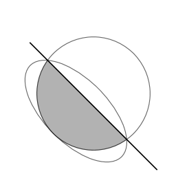
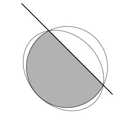
Figure 10.1: The ellipsoid method in action. The shaded region is the intersection of the half-space and the large circle and the ellipse is the minimum volume ellipsoid containing this intersection created using the formula in Lemma 10.3.

Proof of Theorem 10.2.

Let $x_{\star}=\operatornamewithlimits{arg\,min}_{x\in K}f(x)$ and $\delta=\frac{\varepsilon}{\operatorname{diam}(K)}$ and

$$A_{\star}=(1-\delta)x_{\star}+\delta K\subset K\,.$$

Suppose that $x\in A_{\star}$. Then, $\left\|x-x_{\star}\right\|\leq\varepsilon$ and hence $f(x)\leq f(x_{\star})+\varepsilon$ since $f\in\mathscr{F}_{\tiny{\texttt{l}}}$. Furthermore,

$$\operatorname{vol}(A_{\star})=\delta^{d}\operatorname{vol}(K)\,.$$

Let $H_{k}=\{x:\left\langle g_{k},x-z_{k}\right\rangle\leq 0\}$ where $g_{k}\in\partial f(z_{k})$. By convexity of $f$, if $x\in H_{k}^{c}$, then $f(x)\geq f(z_{k})$. By Lemma 10.3,

$$\operatorname{vol}(K_{k_{\star}})\leq\operatorname{vol}(E_{k_{\star}})\leq\gamma^{k_{\star}-1}\operatorname{vol}(E_{1})\leq\gamma^{k_{\star}-1}\leq\delta^{d}\operatorname{vol}(K)\,.$$

Hence there exists a $k\leq k_{\star}$ and $x\in A_{\star}$ such that $\left\langle g_{k},x-z_{k}\right\rangle\geq 0$, which means that $f(x_{\star})+\varepsilon\geq f(x)\geq f(z_{k})$. ∎

10.2  Separation with a surrogate

In this section we explain how to use the optimistic surrogate in place of the subgradient oracle used by Algorithm 19. Let $K$ be a convex body and $f\in\mathscr{F}_{\tiny{\texttt{b}},\tiny{\texttt{l}},\tiny{\texttt{sc}},\tiny{\texttt{sm}}}$ and $x_{\star}=\operatornamewithlimits{arg\,min}_{x\in K}f(x)$. Throughout this section we let

$$\rho =\frac{\lambda r^{2}}{30d} r =\frac{1}{2d} \lambda =\frac{1}{dL^{2}}\,.$$ (10.1)

We will assume we have been given an ellipsoid $E=E(x,A)$ such that

$$E(x,\textstyle{\frac{1}{120d^{3}L}}A)=E(x,\rho dLA)\subset K\subset E(x,A)\,.$$

Note that $E$ does not need to be the minimum volume enclosing ellipsoid of $K$. In order to drive the ellipsoid method you need to find a half-space $H$ such that

• $H\cap E(x,r^{2}A)\neq\emptyset$; and

• $x_{\star}\in H$.

This can be done with a subgradient oracle for $f$ but it can also be found using the optimistic surrogate used in the Chapter 9 and studied extensively Chapter 11. Let $X$ have law $\mathcal{N}(x,\Sigma)$ with $\Sigma=\rho A$ and

$$s(z) =\mathbb{E}\left[\left(1-\frac{1}{\lambda}\right)f(X)+\frac{1}{\lambda}f((1-\lambda)X+\lambda z)\right]\,.$$

$$q(z) =\left\langle s^{\prime}(x),z-x\right\rangle+\frac{1}{6}\left\|z-x\right\|^{2}_{s^{\prime\prime}(x)}\,.$$

Sadly there is no particular reason why $H=\{y:\left\langle s^{\prime}(x),y-x\right\rangle\leq 0\}$ should include $x_{\star}$, which by convexity would be true if we used $f^{\prime}(x)$ instead of $s^{\prime}(x)$. Suppose, however, that we can find a $z$ such that $s(z)\geq f(x_{\star})$ and let $H=\{y:\left\langle s^{\prime}(z),y-z\right\rangle\leq 0\}$. Then, by Lemma 11.1(b)(a),

$$f(x_{\star})\geq s(x_{\star})\geq s(z)+\left\langle s^{\prime}(z),x_{\star}-z\right\rangle\geq f(x_{\star})+\left\langle s^{\prime}(z),x_{\star}-z\right\rangle\,.$$

Therefore $\left\langle s^{\prime}(z),x_{\star}-z\right\rangle\leq 0$ and consequentially $x_{\star}\in H$. We also want $H\cap E(x,r^{2}A)\neq\emptyset$, which can be ensured by choosing $z\in E(x,r^{2}A)$. The following lemma shows that such a point exists.

Lemma 10.4.

Let $\Delta=\mathbb{E}[f(X)]-f(x_{\star})$. Then,

$$\max_{z\in E(x,r^{2}A)}(q(z)+s(x))\geq f(x)+\frac{r\Delta}{2}\,.$$

Proof.

We have

$$\Delta =\mathbb{E}[f(X)]-f(x_{\star})$$

$$\leq s(x)-s(x_{\star})+\frac{1}{\lambda}\operatorname{tr}(s^{\prime\prime}(x)\Sigma)$$ (Proposition 11.5, Lemma 11.1)

$$\leq\left\langle s^{\prime}(x),x-x_{\star}\right\rangle+\frac{1}{\lambda}\operatorname{tr}(s^{\prime\prime}(x)\Sigma) s$$ (Convexity of )

$$\leq\left\|s^{\prime}(x)\right\|_{A}\left\|x-x_{\star}\right\|_{A^{-1}}+\frac{d}{\lambda}\left\|s^{\prime\prime}(x)\right\|_{\Sigma}$$

$$\leq\left\|s^{\prime}(x)\right\|_{A}+\frac{d}{\lambda}\left\|s^{\prime\prime}(x)\right\|_{\Sigma}\,. x_{\star}\in E(x,A)$$ ()

Furthermore,

$$\max_{z\in E(x,r^{2}A)}q(z)=\max_{z\in E(x,r^{2}A)}\left[\left\langle s^{\prime}(x),z-x\right\rangle+\frac{1}{6}\left\|z-x\right\|^{2}_{s^{\prime\prime}(x)}\right]$$

$$\qquad\stackrel{{\scriptstyle\text{\tiny(a)}}}{{\geq}}\max\left(r\left\|s^{\prime}(x)\right\|_{A},\frac{r^{2}}{6}\left\|s^{\prime\prime}(x)\right\|_{A}\right)$$

$$\qquad\stackrel{{\scriptstyle\text{\tiny(b)}}}{{\geq}}f(x)-s(x)-\frac{4}{\lambda}\operatorname{tr}(s^{\prime\prime}(x)\Sigma)+\max\left(r\left\|s^{\prime}(x)\right\|_{A},\frac{r^{2}}{6}\left\|s^{\prime\prime}(x)\right\|_{A}\right)$$

$$\qquad\stackrel{{\scriptstyle\text{\tiny(c)}}}{{\geq}}f(x)-s(x)-\frac{4d}{\lambda}\left\|s^{\prime\prime}(x)\right\|_{\Sigma}+\max\left(r\left\|s^{\prime}(x)\right\|_{A},\frac{r^{2}}{6\rho}\left\|s^{\prime\prime}(x)\right\|_{\Sigma}\right)$$

$$\qquad\stackrel{{\scriptstyle\text{\tiny(d)}}}{{\geq}}f(x)-s(x)+\frac{d}{\lambda}\left\|s^{\prime\prime}(x)\right\|_{\Sigma}+\frac{r}{2}\left\|s^{\prime}(x)\right\|_{A}\,.$$

where in (a) we used the fact that $s^{\prime\prime}(x)\succ\bm{0}$ and various choices of $z$ to maximise either the first or the second term. (b) follows from Proposition 11.5. (c) since $\operatorname{tr}(\cdot)\leq d\left\|\cdot\right\|$ and since $\Sigma=\rho A$. (d) follows since $\max(a,b)\geq(a+b)/2$ and by our choice of the constants $\lambda$, $\rho$ and $r$. Combining the two displays completes the proof. ∎

The lemma shows there exists a $z$ in $E(x,r^{2}A)$ such that a gradient oracle of the surrogate at $z$ will provide a suitable cutting plane. This suggests a clear plan of attack to use the ellipsoid method for bandit convex optimisation:

• Collect data to estimate the quadratic surrogate and maximise over $E(x,r^{2}A)$ to find a critical point.

• Estimate the gradient of the surrogate the critical point and use it to define a cutting plane.

• Combine the above with the ellipsoid method in Algorithm 19.

10.3  Finding a critical point

Lemma 10.4 established the existence of a $z\in E(x,r^{2}A)$ for which $q(z)+s(x)\geq f(x)+\frac{1}{2}r\Delta$. We now show how find a comparable point with zeroth-order access to the loss function $f$. The idea is very simple. We estimate the quadratic $q$ and maximise the estimate. The errors are controlled using the concentration of measure properties established in Chapter 11. There are really only two details:

• The algorithm also needs to output a constant-factor approximation of the gap $q(z)+s(x)-f(x)$ to be used later, which means we need a careful choice of stopping time.

• While the quadratic surrogate $q$ is convex, its estimate is only nearly so. Hence we do not maximise the estimate but a biased version of it that is convex with high probability. Note that maximising a convex function over a convex domain is not normally computationally feasible. Luckily the case where the objective is quadratic and the constraint set is an ellipsoid works out nicely. Read all about it in Note (c).

Theorem 10.5.

Suppose that Algorithm 22 is run with the parameters given in Eq. 10.1 and an ellipsoid $E(x,A)$ such that $E(x,\rho dLA)\subset K$. Then with probability at least $1-n\delta$ the algorithm halts after at most

$$O\left(\frac{d^{5}L^{4}}{\Delta^{2}}\right)\,.$$

queries to the loss function and outputs a point $z\in E(x,r^{2}A)$ and estimate $\theta$ such that

1. $s(z)\geq f(x)+\frac{r\Delta}{4}$.

2. $s(z)-f(x)\in[\frac{1}{2}\theta,2\theta]$.

⬇

1args: $r\in(0,1)$, $\rho\in(0,1)$, $\lambda\in(0,1)$, $E(x,A)$

2let $\Sigma=\rho A$ and $D=\frac{r}{\sqrt{\rho}}$

3for $t=1$ to $\infty$

4 if $t$ is odd:

5 sample $X_{t}$ from $\mathcal{N}(x,\Sigma)$ and observe $Y_{t}=f(X_{t})+\varepsilon_{t}$

6 let $g_{t}=\frac{r(X_{t},x)Y_{t}\Sigma^{-1}(X_{t}-x)}{1-\lambda}$

7 let $H_{t}=\frac{\lambda r(X_{t},x)Y_{t}}{(1-\lambda)^{2}}\left[\frac{\Sigma^{-1}(X_{t}-x)(X_{t}-x)^{\top}\Sigma^{-1}}{(1-\lambda)^{2}}-\Sigma^{-1}\right]$

8 else:

9 play $X_{t}=x$ and observe $Y_{t}=f(x)+\varepsilon_{t}$

10 let $\bar{q}_{t}(y)=\frac{2}{t}\sum_{u=1}^{t}\bm{1}(u\text{ odd})\left[\left\langle g_{u},y-x\right\rangle+\frac{1}{6}\left\|y-x\right\|^{2}_{H_{u}}\right]$

11 let $\bar{f}_{t}=\frac{2}{t}\sum_{u=1}^{t}\bm{1}(u\text{ even})Y_{u}$

12 let $z_{t}=\operatornamewithlimits{arg\,max}_{z\in E(x,r^{2}A)}\bar{q}_{t}(z)+\frac{\lambda L}{6}\sqrt{\frac{d}{t}}\left\|z-x\right\|^{2}_{\Sigma^{-1}}$

13 let $c_{t}=[1+D+(1+1/6)\lambda D^{2}]L\sqrt{\frac{d}{t}}$

14 if $\bar{q}_{t}(z_{t})-\bar{f}_{t}\geq 2c_{t}$: return $z_{t}$ and $\bar{q}_{t}(z_{t})-\bar{f}_{t}$

Algorithm 20 Algorithm for finding critical point

Proof.

Note that for $z\in E(x,r^{2}A)$ we have

$$\left\|z-x\right\|_{\Sigma^{-1}}\leq\frac{r}{\sqrt{\rho}}\,.$$

By a union bound and Proposition 11.18, with probability at least $1-n\delta/2$ the following holds for all even $1\leq t\leq n$,

$$\max_{y\in E(x,r^{2}A)}\left|q(y)-\bar{q}_{t}(y)\right|\leq\left[D+\lambda D^{2}\right]L\sqrt{\frac{2d}{t}}\,.$$ (10.2)

Since the noise is subgaussian we also have with probability at least $1-n\delta/2$ that for all even $1\leq t\leq n$,

$$\left|\bar{f}_{t}-f(x)\right|\leq\sqrt{\frac{2L}{t}}\,.$$ (10.3)

Another union bound shows that both Eq. 10.2 and Eq. 10.3 hold with probability $1-n\delta$. We assume this event occurs for the remainder of the proof. Suppose the algorithm stops after round $t$. Then,

$$\theta_{t} =\bar{q}_{t}(z_{t})-\bar{f}_{t}\geq q(z_{t})-f(x)-c_{t}\geq q(z_{t})-f(x)-\frac{\theta_{t}}{2}\,,$$

which implies that $q(z_{t})-f(x)\leq\frac{3}{2}\theta$. Reversing the argument yields $q(z_{t})-f(x)\geq\frac{\theta}{2}$. Furthermore,

$$\theta_{t} =\bar{q}_{t}(z_{t})-\bar{f}_{t}$$

$$=\max_{z\in E(x,r^{2}A)}\bar{q}_{t}(z)-\bar{f}_{t}$$

$$\geq\max_{z\in E(x,r^{2}A)}q(z)-f(x)-c_{t}$$

$$\geq\frac{r\Delta}{2}-c_{t}$$ (By Lemma 10.4)

$$\geq\frac{r\Delta}{2}-\frac{\theta_{t}}{2}\,.$$ (Algorithm has halted)

Finally, we need to show that the algorithm halts once $t$ is large enough. Concretely, once $c_{t}\leq\frac{r\Delta}{6}$, then repeating the argument above to the second last line shows that $\theta_{t}\geq\frac{r\Delta}{3}=2c_{t}$ and hence the algorithm halts. The claim follows from the definition of $c_{t}$. ∎

10.4  Estimating the cutting plane

Theorem 10.6.

Suppose that Algorithm 21 is run with the parameters given in Eq. 10.1 and an ellipsoid $E(x,A)$ such that $E(x,\rho dLA)\subset K$. Then with probability at least $1-(n+1)\delta$ the algorithm halts after at most

$$O\left(\frac{d^{6}L^{4}}{\Delta^{2}}\right)\,.$$

queries to the loss function and outputs a half-space $H$ such that $H\cap E(x,r^{2}A)$ is nonempty and $x_{\star}\in H$.

Proof.

With probability at least $1-n\delta$,

1. $s(z)\geq f(x)+\frac{r\Delta}{4}$.

2. $s(z)-f(x)\in[\frac{\theta}{2},2\theta]$.

Therefore, by convexity of $s$ (Lemma 11.1(a)),

$$\left\langle s^{\prime}(z),x_{\star}-z\right\rangle\leq s(x_{\star})-s(z)\leq f(x)-s(z)\,.$$

On the other hand, by Proposition 11.21, with probability at least $1-\delta$, size=,color=red!20!white,]Tor: check logarithmic factor

$$\left\langle\bar{g},x_{\star}-z\right\rangle \leq\left\langle s^{\prime}(z),x_{\star}-z\right\rangle+\left\|x_{\star}-z\right\|_{\Sigma^{-1}}L\sqrt{\frac{1}{m}}$$

$$=\left\langle s^{\prime}(z),x_{\star}-z\right\rangle+\left\|x_{\star}-z\right\|_{A^{-1}}L\sqrt{\frac{1}{m\rho}}$$

$$\leq\left\langle s^{\prime}(z),x_{\star}-z\right\rangle+L\sqrt{\frac{1}{m\rho}}$$

$$\leq f(x)-s(z)+\frac{\theta}{2}$$

$$\leq 0\,.$$

∎

⬇

1args: $r\in(0,1)$, $\rho\in(0,1)$, $\lambda\in(0,1)$, $E(x,A)$

2run Algorithm 20 and obtain $z\in E(x,r^{2}A)$ and $\theta>0$

3let $m=\left\lceil\frac{4L^{2}}{\rho\theta^{2}}\right\rceil$ and $\Sigma=\rho A$

4for $t=1$ to $m$:

5 sample $X_{t}\sim\mathcal{N}(x,\Sigma)$ and observe $Y_{t}=f(X_{t})+\varepsilon_{t}$

6 let $g_{t}=r(X_{t},z)Y_{t}\Sigma^{-1}\left(\frac{X_{t}-\lambda z}{1-\lambda}-\mu\right)$

7let $\bar{g}=\frac{1}{m}\sum_{t=1}^{m}g_{t}$

8return $H=\{y:\left\langle\bar{g},y-z\right\rangle\leq 0\}$

Algorithm 21 Algorithm for finding critical point

10.5  Algorithm and analysis outline

⬇

1args: $r\in(0,1)$, $\rho\in(0,1)$, $\lambda\in(0,1)$

2let $K_{1}=K$

3for $k=1$ to $\infty$:

4 let $E_{k}=\operatorname{\textsc{mvee}}(K_{k})$

5 get $H_{k}$ from Algorithm 21 with input $r,\rho,\lambda,E_{k}$

6 let $K_{k+1}=K_{k}\cap H_{k}$

Algorithm 22 Ellipsoid method for bandit convex optimisation

Theorem 10.7.

With probability at least $1-n^{2}\delta$ the regret of Algorithm 22 is at most

$$\textrm{Reg}_{n}=O\left(d^{4}L^{2.5}\sqrt{n}\right)\,.$$

Proof sketch.

With high probability, the number of episodes is at most $O(d^{2}L)$. Let $n_{k}$ be the number of rounds in episode $k$. By Theorem 10.5, with high probability

$$n_{k}=O\left(\frac{d^{6}L^{4}}{\Delta_{k}^{2}}\right)\,,$$

where $\Delta_{k}$ is the expected instantaneous regret incurred by each query in episode $k$. Therefore the regret in episode $k$ is bounded by

$$n_{k}\Delta_{k}=O\left(d^{3}L^{2}\sqrt{n_{k}}\right)\,.$$

With probability at least $1-\delta$,

$$\textrm{Reg}_{n} =\sum_{t=1}^{n}(f(X_{t})-f(x_{\star}))\leq\sum_{t=1}^{n}(\mathbb{E}_{t-1}[f(X_{t})]-f(x_{\star}))+\sqrt{nL}\,.$$

Therefore,

$$\textrm{Reg}_{n} \leq\sum_{k=1}^{k_{\max}}n_{k}\Delta_{k}+\sqrt{nL}$$

$$\leq\sum_{k=1}^{k_{\max}}O\left(d^{3}L^{2}\sqrt{n_{k}}\right)+\sqrt{nL}$$

$$\leq O\left(d^{3}L^{2}\sqrt{k_{\max}\sum_{k=1}^{k_{\max}}n_{k}}\right)+\sqrt{nL}$$

$$=O\left(d^{4}L^{2.5}\sqrt{n}\right)\,.$$

∎

Figure 10.2: The ellipsoid method in action. The outer ellipsoid is $E(x,A)$ and the inner one is $E(x,r^{2}A)$. The lightly shaded polytope is the current constraint set and the more deeply shaded polytope is the new one after a cut has been made. Note that $K\subset E(x,A)$ is necessary but we do not demand that $E(x,r^{2}A)\subset K$. The algorithm is playing with overwhelming probability in the region near the origin.

10.6  Notes

1. The ellipsoid method was introduced and refined by Shor (1977); Yudin and Nemirovskii (1977, 1976) and then made famous by Khachiyan (1979) who modified the method to show that linear programming is polynomial time. The book by Grötschel et al. (2012) covers everything you need to know about the ellipsoid method.

2. Algorithm 22 is inspired by Lattimore and György (2021a), who use the same surrogate loss in combination with the ellipsoid method to prove a bound on the regret of $d^{4.5}\sqrt{n}$. The main difference is that Algorithm 22 finds the point $z$ by directly optimising the estimated quadratic surrogate, while Lattimore and György (2021a) use a random search procedure that is slightly less efficient.

3. Algorithm 22 needs to maximise a convex quadratic over an ellipsoid. Generally speaking convex maximisation is computationally hard, but for this special case you will find the method of Lagrange multipliers yields a solution for which the computational complexity involves a line search over a single Lagrange multiplier.

4. For simplicity the algorithm finds the minimum volume ellipsoid $\operatorname{\textsc{mvee}}(K_{k}\cap H_{k})$. This is generally computationally hard, even when $K_{k}$ is a polytope. Fortunately all that is required is to find an ellipsoid $E=E(x,A)$ such that $E(x,\rho dLA)\subset K\subset E(x,A)$ and this is computationally efficient when $K$ is given by a separation oracle as explained by Grötschel et al. (2012, Chapter 4) or Lattimore and György (2021a) for this specific application.

5. Like Algorithm 18, the parameters in Algorithm 22 depend on large unspecified logarithmic factors. Like that algorithm, you should probably just drop all logarithmic factors. Furthermore, exact confidence intervals should be replaced by standard statistical tests.

6. The ellipsoid method has a bad reputation from a practical perspective. The main problems are numerical instability (the ellipsoid becomes poorly conditioned) and the fact that the convergence rate in practice usually more-or-less matches the theory.

7. Another standard cutting plane method for convex optimisation is the center of gravity method, which starts with $K_{1}=K$ and updates $K_{k+1}$ from $K_{k}$ by finding $x_{k}=\frac{1}{\operatorname{vol}(K_{k})}\int_{K_{k}}x\operatorname{d}\!x$ and then using a gradient oracle: $K_{k+1}=\{x\in K_{k}:\left\langle g_{k},x-x_{k}\right\rangle\leq 0\}$ with $g_{k}\in\partial f(x_{k})$. By Grünbaum’s inequality (Artstein-Avidan et al., 2015), $\operatorname{vol}(K_{k+1})\leq(1-1/e)\operatorname{vol}(K_{k})$. This means the center of gravity method requires a factor of $d$ fewer iterations than the ellipsoid method. A natural question is whether or not the techniques in this chapter can be modified to use the center of gravity method rather than the ellipsoid method.

Chapter 11  Gaussian optimistic smoothing

The purpose of this chapter is to introduce and analyse the surrogate loss functions used in Chapters 9 and 10. We try to make the results here as general as possible so that you may use them in your own algorithms and analysis. Throughout we make the following assumptions:

1. The loss functions are twice differentiable; and

2. Loss functions are in $\mathscr{F}_{\tiny{\texttt{b}},\tiny{\texttt{sm}},\tiny{\texttt{sc}},\tiny{\texttt{e}}}$ with domain $K$.

Since the losses are in $\mathscr{F}_{\tiny{\texttt{e}}}$ we can and will assume that the losses are defined on all of $\mathbb{R}^{d}$. Note, however, that the extension only preserves strong convexity and smoothness to $\mathbb{R}^{d}$. Boundedness only holds on the domain $K$.

Because the analysis is quite intricate and we are not so concerned by constants and logarithmic factors, we let $L$ be a large logarithmic factor. Precisely,

$$L=C\left[1+\log\max(n,d,\beta/\alpha,\operatorname{diam}(K),1/\delta,\operatorname{lip}_{K}(F))\right]\,,$$

where $C>0$ is a large non-specified universal positive constant. We also let $(C_{k})$ be a collection of $k$-dependent universal positive constants. In case you want a quick summary of the results, read until the end of this section for the basic definitions and then head directly to Section 11.9.

Suppose that $X$ is a random vector in $\mathbb{R}^{d}$. We are interested in the problem of estimating the entire function $f\in\mathscr{F}_{\tiny{\texttt{b}},\tiny{\texttt{sm}},\tiny{\texttt{sc}},\tiny{\texttt{e}}}$ from a single observation $Y=f(X)+\varepsilon$ where $\left\|\varepsilon\right\|_{\psi_{2}}\leq 1$. Given a parameter $\lambda\in(0,\frac{1}{d+1})$, define the surrogate by

$$s(x)=\mathbb{E}\left[\left(1-\frac{1}{\lambda}\right)f(X)+\frac{1}{\lambda}f((1-\lambda)X+\lambda x)\right]\,.$$ (11.1)

For the remainder we assume that the law of $X$ is Gaussian with mean $\mu$ and covariance $\Sigma\succ\bm{0}$. The density of $X$ with respect to the Lebesgue measure is

$$p(x)=\left(\frac{1}{2\pi}\right)^{\frac{d}{2}}\sqrt{\det\Sigma^{-1}}\exp\left(-\frac{1}{2}\left\|x-\mu\right\|^{2}_{\Sigma^{-1}}\right)\,.$$

The quadratic surrogate is

$$q(x)=\left\langle s^{\prime}(\mu),x-\mu\right\rangle+\frac{1}{6}\left\|x-\mu\right\|^{2}_{s^{\prime\prime}(\mu)}\,,$$ (11.2)

which is related to the second-order expansion of $s$ at $\mu$ but the zeroth-order term is dropped and the leading constant of the quadratic term is $\frac{1}{6}$ rather than $\frac{1}{2}$.

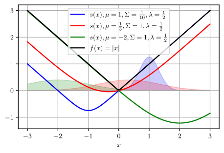
Figure 11.1: The figure plots the surrogate for different choices of $\mu$ and $\Sigma$ with $\lambda=\frac{1}{2}$ in all figures. Notice that the surrogate is always optimistic in the sense that $s(x)\leq f(x)$ for all $x$. The surrogate is a reasonable approximation of $f$ on the confidence region $\mu\pm\sqrt{\Sigma}$. For the blue and green curves the approximation is extremely good indeed, which you should expect because $f$ is approximately linear on the corresponding confidence regions.

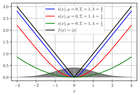
Figure 11.2: The figure plots the surrogate for $\mu$ and $\Sigma$ constant and different choices of $\lambda$. You can see that smaller $\lambda$ yields a smoother surrogate, but also one that has more approximation error.

11.1  Elementary properties

An immediate consequence of the definitions is that $s$ is convex and a lower bound on $f$.

Lemma 11.1.

The function $s$ is infinitely differentiable and

1. $s$ is convex; and

2. $s(x)\leq f(x)$ for all $x\in\mathbb{R}^{d}$; and

3. $\lambda\alpha\leq\left\|s^{\prime\prime}(x)\right\|\leq\lambda\beta$ for all $x$.

Proof.

Part (a) is immediate from the convexity of $f$. Part (b) also uses convexity of $f$ and Jensen’s inequality. Part (c) follows immediately from the definition of $s$ and the convexity of norms. ∎

Perhaps the most important property of $s$ is that it is not too far below $f$ on an ellipsoidal region about $\mu$. Establishing this is quite involved, however, and relies on a better understanding of the Hessian of $s$.

11.2  Properties of the gradient

We have assumed that $f\in\mathscr{F}_{\tiny{\texttt{b}},\tiny{\texttt{sm}},\tiny{\texttt{sc}},\tiny{\texttt{e}}}$ and $\operatorname{dom}(f)=K$. This means that $f$ is $\beta$-smooth on all of $\mathbb{R}^{d}$. With this information we can control the gradients of $s$ in terms of those of $f$.

Proposition 11.2.

$\operatorname{lip}_{K}(s)\leq\operatorname{lip}_{K}(f)+\beta\sqrt{d\mathbb{P}(X\notin K)\left\|\Sigma\right\|}$.

Proof.

Let $d(x,K)=\inf_{y\in K}\left\|x-y\right\|$. Since $f$ is $\beta$-smooth, for any $x\in K$,

$$\left\|s^{\prime}(x)\right\| =\left\|\mathbb{E}[f^{\prime}((1-\lambda)X+\lambda x)]\right\|$$

$$\leq\operatorname{lip}_{K}(f)+\beta\mathbb{E}\left[d_{K}((1-\lambda)X+\lambda x)\right]$$

$$\leq\operatorname{lip}_{K}(f)+\beta\mathbb{E}\left[d_{K}(X)\right]$$

$$\leq\operatorname{lip}_{K}(f)+\beta\mathbb{E}\left[\bm{1}_{K^{c}}(X)\|X-\mu\|\right]$$

$$\leq\operatorname{lip}_{K}(f)+\beta\sqrt{\mathbb{P}(X\notin K)\mathbb{E}[\|X-\mu\|^{2}]}$$

$$\leq\operatorname{lip}_{K}(f)+\beta\sqrt{d\mathbb{P}(X\notin K)\|\Sigma\|}\,.\qed$$

Generally speaking we will be designing algorithms where $\mathbb{P}(X\notin K)$ is miniscule and in these cases the surrogate is nearly as Lipschitz as $f$.

11.3  Properties of the Hessian

The next important property is a kind of continuity of the Hessian.

Proposition 11.3.

If $\lambda\left\|x-y\right\|_{\Sigma^{-1}}\leq L^{-1/2}$, then $s^{\prime\prime}(x)\preceq 3s^{\prime\prime}(z)$.

Proof.

Let $\varepsilon=\frac{\lambda(x-y)}{1-\lambda}$ and assume, by changing coordinates, that $\mu=\bm{0}$. By definition,

$$s^{\prime\prime}(x) =\lambda\mathbb{E}\left[f^{\prime\prime}((1-\lambda)X+\lambda x)\right]$$

$$=\lambda\int_{\mathbb{R}^{d}}f^{\prime\prime}((1-\lambda)z+\lambda x)p(z)\operatorname{d}\!z$$

$$=\lambda\int_{\mathbb{R}^{d}}f^{\prime\prime}((1-\lambda)w+\lambda y)p\left(w+\frac{\lambda(y-x)}{1-\lambda}\right)\operatorname{d}\!w$$

$$=\lambda\int_{\mathbb{R}^{d}}f^{\prime\prime}((1-\lambda)w+\lambda y)\frac{p\left(w+\frac{\lambda(y-x)}{1-\lambda}\right)}{p(w)}p(w)\operatorname{d}\!w$$

$$=\lambda\int_{\mathbb{R}^{d}}f^{\prime\prime}((1-\lambda)w+\lambda y)\frac{p\left(w+\varepsilon\right)}{p(w)}p(w)\operatorname{d}\!w\,,$$ (11.3)

The density ratio is

$$\frac{p(w+\varepsilon)}{p(w)} =\exp\left(-\frac{1}{2}\left\|w+\varepsilon\right\|^{2}_{\Sigma^{-1}}+\frac{1}{2}\left\|w\right\|^{2}_{\Sigma^{-1}}\right)$$

$$=\exp\left(-\frac{1}{2}\left\|\varepsilon\right\|^{2}_{\Sigma^{-1}}-\left\langle w,\varepsilon\right\rangle_{\Sigma^{-1}}\right)\,.$$

Next, let $A=\left\{w:-\frac{1}{2}\left\|\varepsilon\right\|^{2}_{\Sigma^{-1}}-\left\langle w,\varepsilon\right\rangle_{\Sigma^{-1}}\leq\log(2)\right\}$. Decomposing the integral in Eq. 11.3 into the integral over $A$ and $A^{c}$,

$$\lambda\int_{A}f^{\prime\prime}((1-\lambda)w+\lambda y)p(w+\varepsilon)\operatorname{d}\!w \leq 2\lambda\int_{A}f^{\prime\prime}((1-\lambda)w+\lambda y)p(w)\operatorname{d}\!w$$

$$\leq 2\lambda\int_{\mathbb{R}^{d}}f^{\prime\prime}((1-\lambda)w+\lambda y)p(w)\operatorname{d}\!w$$

$$=2s^{\prime\prime}(y)\,.$$

Moving now to bound the integral over $A^{c}$:

$$\left\|\lambda\int_{A^{c}}f^{\prime\prime}((1-\lambda)w+\lambda y)p(w+\varepsilon)\operatorname{d}\!w\right\|\leq\lambda\beta\int_{A^{c}}p(w+\varepsilon)\operatorname{d}\!w$$

$$\qquad=\lambda\beta\mathbb{P}(X-\varepsilon\in A^{c})$$

$$\qquad=\lambda\beta\mathbb{P}\left(-\frac{1}{2}\left\|\varepsilon\right\|^{2}_{\Sigma^{-1}}-\left\langle X-\varepsilon,\Sigma^{-1}\varepsilon\right\rangle>\log(2)\right)$$

$$\qquad\leq\lambda\beta\exp\left(-\frac{\left(\log(2)-\frac{1}{2}\left\|\varepsilon\right\|^{2}_{\Sigma^{-1}}\right)^{2}}{2\left\|\varepsilon\right\|^{2}_{\Sigma^{-1}}}\right)\,.$$

Therefore,

$$s^{\prime\prime}(x) \preceq 2s^{\prime\prime}(y)+\lambda\beta\exp\left(-\frac{\left(\tau-\frac{1}{2}\left\|\varepsilon\right\|^{2}_{\Sigma^{-1}}\right)^{2}}{2\left\|\varepsilon\right\|^{2}_{\Sigma^{-1}}}\right)\mathds{1}\preceq 3s^{\prime\prime}(y)\,,$$

where the last inequality follows for large enough $L$ since

$$\left\|\varepsilon\right\|^{2}_{\Sigma^{-1}}=\left(\frac{\lambda}{1-\lambda}\right)^{2}\left\|x-y\right\|^{2}_{\Sigma^{-1}}\leq\frac{1}{L(1-\lambda)^{2}}$$

and using from Lemma 11.1(c) that $s^{\prime\prime}(y)\succeq\lambda\alpha\mathds{1}$. ∎

11.4  Properties of the quadratic surrogate

Obviously $q$ inherits convexity from $s$. Optimism is not inherited everywhere, but $q$ is optimistic on a ellipsoidal region about $\mu$, which follows from the continuity properties of the Hessian of $s$ and the definition of $q$.

Proposition 11.4.

Suppose that $\lambda\left\|x-\mu\right\|_{\Sigma^{-1}}\leq\frac{1}{L}$, then $s(\mu)-s(x)\leq q(\mu)-q(x)$.

Proof.

That $s\leq f$ we established already in Lemma 11.1(b). For the first inequality, by Proposition 11.3, $3s^{\prime\prime}(y)\succeq s^{\prime\prime}(\mu)$ for all $y\in[\mu,x]$. Therefore, by Taylor’s theorem,

$$s(x) =s(\mu)+\left\langle s^{\prime}(\mu),x-\mu\right\rangle+\frac{1}{2}\left\|x-\mu\right\|^{2}_{s^{\prime\prime}(y)}$$

$$\geq s(\mu)+\left\langle s^{\prime}(\mu),x-\mu\right\rangle+\frac{1}{6}\left\|x-\mu\right\|^{2}_{s^{\prime\prime}(\mu)}$$

$$=s(\mu)+q(x)\,.$$

The result follows by rearranging and because $q(\mu)=0$. ∎

11.5  Lower bound

We have shown that $s\leq f$ holds everywhere. We now show that $s$ is reasonably close to $f$ at $\mu$.

Proposition 11.5.

Provided that $\lambda\leq\frac{1}{dL^{2}}$,

$$f(\mu)\leq\mathbb{E}[f(X)]\leq s(\mu)+\frac{4}{\lambda}\operatorname{tr}(s^{\prime\prime}(\mu)\Sigma)\,.$$

Proof.

The first inequality is immediate from Jensen’s inequality. Let $Z$ be a random variable that is independent of $X$ and has law $\mathcal{N}(\mu,\rho^{2}\Sigma)$ where $\rho^{2}=\frac{2-\lambda}{\lambda}$ is chosen so that $(1-\lambda)^{2}+\lambda^{2}\rho^{2}=1$. Then

$$\mathbb{E}[s(Z)] =\mathbb{E}\left[\left(1-\frac{1}{\lambda}\right)f(X)+\frac{1}{\lambda}f((1-\lambda)X+\lambda Z)\right]$$

$$=\mathbb{E}\left[\left(1-\frac{1}{\lambda}\right)f(X)+\frac{1}{\lambda}f(X)\right]$$

$$=\mathbb{E}\left[f(X)\right]\,,$$

where we used the fact that $(1-\lambda)X+\lambda Z$ has the same law as $X$. Let us now compare $\mathbb{E}[s(Z)]$ to $s(\mu)$. By Taylor’s theorem there exists a $\xi_{z}\in[\mu,z]$ such that

$$\mathbb{E}[s(Z)] =\mathbb{E}\left[s(\mu)+s^{\prime}(\mu)^{\top}(z-\mu)+\frac{1}{2}\left\|Z-\mu\right\|^{2}_{s^{\prime\prime}(\xi_{Z})}\right]\,.$$

By Proposition 11.3, if $z$ is close enough to $\mu$, then $s^{\prime\prime}(z)$ is close to $s^{\prime\prime}(\mu)$. Define

$$A =\left\{z\in\mathbb{R}^{d}:\lambda\left\|z-\mu\right\|_{\Sigma^{-1}}\leq L^{-1/2}\right\}\,.$$

Note that $\mu\in A$ and that $A$ is convex. Hence, if $z\in A$, then $\xi_{z}\in A$ and $s^{\prime\prime}(\xi_{z})\leq 3s^{\prime\prime}(\mu)$. Therefore

$$\mathbb{E}[s(Z)] =\mathbb{E}\left[s(\mu)+s^{\prime}(\mu)^{\top}(Z-\mu)+\frac{1}{2}\left\|Z-\mu\right\|^{2}_{s^{\prime\prime}(\xi_{Z})}\right]$$

$$=s(\mu)+\mathbb{E}\left[\frac{1}{2}\left\|Z-\mu\right\|^{2}_{s^{\prime\prime}(\xi_{Z})}\right] \mathbb{E}[Z]=\mu$$ Since

$$\leq s(\mu)+\frac{3}{2}\mathbb{E}\left[\left\|Z-\mu\right\|^{2}_{s^{\prime\prime}(\mu)}\right]+\frac{1}{2}\mathbb{E}\left[\left\|Z-\mu\right\|^{2}_{s^{\prime\prime}(z)}\bm{1}_{A^{c}}(Z)\right]$$

$$=s(\mu)+\frac{3\rho^{2}}{2}\operatorname{tr}(s^{\prime\prime}(\mu)\Sigma)+\frac{1}{2}\mathbb{E}\left[\left\|Z-\mu\right\|^{2}_{s^{\prime\prime}(\xi_{Z})}\bm{1}_{A^{c}}(Z)\right]\,.$$

The error term is bounded by showing that $\mathbb{P}(A^{c})$ is miniscule. Let $W=\Sigma^{-1/2}(X-\mu)$ and bound

$$\mathbb{E}\left[\frac{1}{2}\left\|Z-\mu\right\|^{2}_{s^{\prime\prime}(\xi_{z})}\bm{1}_{A^{c}}(Z)\right] \leq\frac{\beta}{2}\sqrt{\mathbb{E}\left[\left\|Z-\mu\right\|^{4}\right]\mathbb{P}(Z\notin A)}$$

$$=\frac{\beta}{2}\sqrt{\mathbb{E}\left[\left\|Z-\mu\right\|^{4}\right]\mathbb{P}\left(\left\|W\right\|^{2}\geq\frac{1}{\lambda^{2}\rho^{2}L}\right)}$$

$$\leq\frac{\rho^{2}\beta\operatorname{tr}(\Sigma)}{2}\sqrt{3\mathbb{P}\left(\left\|W\right\|^{2}\geq\frac{1}{\lambda^{2}\rho^{2}L}\right)}$$

$$\leq\frac{\beta\operatorname{tr}(\Sigma)}{\lambda}\sqrt{3\mathbb{P}\left(\left\|W\right\|^{2}\geq\frac{1}{\lambda^{2}\rho^{2}L}\right)}\,,$$

where in the second inequality we used Proposition A.2 and the final inequality follows from the definition of $\rho^{2}=\frac{2-\lambda}{\lambda}$. Finally, by Lemma B.3, $\left\|\left\|W\right\|^{2}\right\|_{\psi_{1}}\leq 3d$ and by Lemma B.1,

$$\mathbb{P}\left(\left\|W\right\|^{2}\geq\frac{1}{\lambda^{2}\rho^{2}L}\right) \leq\exp\left(-\frac{1}{3d\lambda^{2}\rho^{2}L}\right)\leq\exp\left(-\frac{1}{6d\lambda L}\right)\,.$$

Combining everything and naively simplifying shows that

$$\mathbb{E}[f(X)] \leq s(\mu)+\frac{3}{\lambda}\operatorname{tr}(s^{\prime\prime}(\mu)\Sigma)+\frac{3\beta\operatorname{tr}(\Sigma)}{\lambda}\sqrt{\exp\left(-\frac{L}{6}\right)}$$

$$\leq s(\mu)+\frac{3}{\lambda}\operatorname{tr}(s^{\prime\prime}(\mu)\Sigma)+\alpha\operatorname{tr}(\Sigma)$$

$$\leq s(\mu)+\frac{4}{\lambda}\operatorname{tr}(s^{\prime\prime}(\mu)\Sigma)\,.\qed$$

11.6  Estimation

The surrogate function can be estimated from $X$ and $Y$ using a change of measure. Precisely,

$$s(z) =\int_{\mathbb{R}^{d}}\left(\left(1-\frac{1}{\lambda}\right)f(x)+\frac{1}{\lambda}f((1-\lambda)x+\lambda z)\right)p(x)\operatorname{d}\!x$$

$$=\int_{\mathbb{R}^{d}}\left(1-\frac{1}{\lambda}+\frac{p\left(\frac{x-\lambda z}{1-\lambda}\right)}{\lambda(1-\lambda)^{d}p(x)}\right)f(x)p(x)\operatorname{d}\!x$$

$$=\int_{\mathbb{R}^{d}}\left(1-\frac{1}{\lambda}+\frac{r(x,z)}{\lambda}\right)f(x)p(x)\operatorname{d}\!x\,,$$ (11.4)

where $r(z)$ is the change of measure defined by

$$r(x,z)=\left(\frac{1}{1-\lambda}\right)^{d}\frac{p\left(\frac{x-\lambda z}{1-\lambda}\right)}{p(x)}\,.$$ (11.5)

From Eq. 11.4 it follows that an unbiased estimator of $s(z)$ using the data $(X,Y)$ is

$$\hat{s}(z)=\left(1-\frac{1}{\lambda}+\frac{r(X,z)}{\lambda}\right)Y\,.$$

Proposition 11.6.

$\mathbb{E}[\hat{s}(z)]=s(z)$.

Note that while $s$ is convex, $x\mapsto\hat{s}(x)$ need not be (see Figure 11.3). One may also want to estimate the gradient and Hessian of the surrogate. Natural unbiased estimates are

$$\hat{s}^{\prime}(z) =r(X,z)Y\Sigma^{-1}\left(\frac{X-\lambda z}{1-\lambda}-\mu\right)\,.$$

$$\hat{s}^{\prime\prime}(z) =\frac{\lambda r(X,z)Y}{(1-\lambda)^{2}}\left[\Sigma^{-1}\left(\frac{X-\lambda z}{1-\lambda}-\mu\right)\left(\frac{X-\lambda z}{1-\lambda}-\mu\right)^{\top}\Sigma^{-1}-\Sigma^{-1}\right]\,.$$

Generally speaking we are most interested in estimating gradients and Hessians of the surrogate at $\mu$, which satisfy

$$\hat{s}^{\prime}(\mu) =\frac{r(X,\mu)Y\Sigma^{-1}(X-\mu)}{1-\lambda}\,.$$

$$\hat{s}^{\prime\prime}(\mu) =\frac{\lambda r(X,\mu)Y}{(1-\lambda)^{2}}\left[\frac{\Sigma^{-1}(X-\mu)(X-\mu)^{\top}\Sigma^{-1}}{(1-\lambda)^{2}}-\Sigma^{-1}\right]\,.$$

Proposition 11.7.

The following hold:

1. $\mathbb{E}[\hat{s}^{\prime}(z)]=s^{\prime}(z)$; and

2. $\mathbb{E}[\hat{s}^{\prime\prime}(z)]=s^{\prime\prime}(z)$.

The identity for the unbiased estimator of the Hessian of the surrogate also gives us an opportunity to bound the magnitude of the Hessian. In general the basic identity in Lemma 11.1(c) is not improvable. But a bound in terms of the covariance is possible:

Proposition 11.8.

$\left\|\Sigma^{1/2}s^{\prime\prime}(\mu)\Sigma^{1/2}\right\|\leq 4\lambda d\sqrt{\mathbb{E}[f((1-\lambda)X+\lambda\mu)^{2}]}$.

Proof.

Assume without loss of generality that $\mu=\bm{0}$. Then,

$$\left\|\Sigma^{1/2}s^{\prime\prime}(\mu)\Sigma^{1/2}\right\| =\left\|\int_{\mathbb{R}^{d}}\frac{\lambda r(x,\mu)f(x)}{(1-\lambda)^{2}}\left[\frac{\Sigma^{-1/2}xx^{\top}\Sigma^{-1/2}}{(1-\lambda)^{2}}-\mathds{1}\right]p(x)\operatorname{d}\!x\right\|$$

$$=\left\|\int_{\mathbb{R}^{d}}\frac{\lambda f((1-\lambda)x)}{(1-\lambda)^{2}}\left[\Sigma^{-1/2}xx^{\top}\Sigma^{-1/2}-\mathds{1}\right]p(x)\operatorname{d}\!x\right\|$$

$$\leq\int_{\mathbb{R}^{d}}\left|\frac{\lambda f((1-\lambda)x)}{(1-\lambda)^{2}}\right|\left\|\Sigma^{-1/2}xx^{\top}\Sigma^{-1/2}-\mathds{1}\right\|p(x)\operatorname{d}\!x$$

$$\leq\frac{\lambda}{(1-\lambda)^{2}}\sqrt{\mathbb{E}[f((1-\lambda)X)^{2}]\mathbb{E}\left[\left\|WW^{\top}-\mathds{1}\right\|^{2}\right]}$$

$$=\frac{\lambda}{(1-\lambda)^{2}}\sqrt{(d^{2}+1)\mathbb{E}[f((1-\lambda)X)^{2}]}\,,$$

where in the first inequality we used convexity of the spectral norm (all norms), in the second we used Cauchy-Schwarz and the last follows from Proposition A.2 and because $\left\|WW^{\top}-\mathds{1}\right\|^{2}=(\left\|W\right\|^{2}-1)^{2}$. ∎

11.7  Concentration ()

In this section we explore the tail behaviour of the estimators in the previous section. Almost all of the results here are only used as technical lemmas in the next section and the proofs are endless applications of Cauchy-Schwarz and the tail bounds in Appendix B. The only fundamental result is Lemma 11.15, so if you only want to read one proof, read that one. We begin with a simple lemma:

Lemma 11.9.

For all $x,z\in\mathbb{R}^{d}$, $r(x,z)\leq 3\exp\big{(}\frac{\lambda}{(1-\lambda)^{2}}\left\langle x-\mu,z-\mu\right\rangle_{\Sigma^{-1}}\big{)}$.

Proof.

Let us assume without loss of generality that $\mu=\bm{0}$. By definition,

$$r(x,z) =\frac{p\left(\frac{x-\lambda z}{1-\lambda}\right)}{(1-\lambda)^{d}p(x)}$$

$$=\frac{1}{(1-\lambda)^{d}}\exp\left(-\frac{1}{2}\left\|\frac{x-\lambda z}{1-\lambda}\right\|^{2}_{\Sigma^{-1}}+\frac{1}{2}\left\|x\right\|^{2}_{\Sigma^{-1}}\right)$$

$$\leq 3\exp\left(-\frac{1}{2}\left\|\frac{x-\lambda z}{1-\lambda}\right\|^{2}_{\Sigma^{-1}}+\frac{1}{2}\left\|x\right\|^{2}_{\Sigma^{-1}}\right)$$

$$\leq 3\exp\left(\frac{\lambda\left\langle x,z\right\rangle_{\Sigma^{-1}}}{(1-\lambda)^{2}}\right)\,.\qed$$

The next lemma shows that $z\mapsto r(x,z)$ has a bounded gradient close to $\mu$.

Lemma 11.10.

Let $r(z)=r(x,z)$ and suppose that

1. $\lambda\left\|z-\mu\right\|_{\Sigma^{-1}}\leq 1/\sqrt{dL}$.

2. $\left\|x-\mu\right\|_{\Sigma^{-1}}\leq\sqrt{dL}$.

Then $\left\|r^{\prime}(z)\right\|\leq C\lambda\sqrt{\left\|\Sigma^{-1}\right\|dL}$.

Proof.

Assume without loss of generality that $\mu=\bm{0}$. Then,

$$\left\|r^{\prime}(z)\right\| =\frac{\lambda r(z)}{(1-\lambda)^{2}}\left\|\Sigma^{-1}(x-\lambda z)\right\|$$

$$\leq\frac{\lambda r(z)}{(1-\lambda)^{2}}\sqrt{\left\|\Sigma^{-1}\right\|}\left\|x-\lambda z\right\|_{\Sigma^{-1}}$$

$$\leq C\lambda\sqrt{\left\|\Sigma^{-1}\right\|dL}\,.\qed$$

Later we need some conservative upper bounds on the moments of the various estimators. The easiest way to obtain these is to bound the moments of the constituent parts and combine them using Hölder’s inequality.

Lemma 11.11.

For any $k\geq 1$, $\mathbb{E}[r(X,x)^{k}]\leq C_{k}\exp\left(C_{k}\lambda^{2}\left\|x-\mu\right\|^{2}_{\Sigma^{-1}}\right)$.

Proof.

By Lemma 11.9 and Proposition A.2,

$$\mathbb{E}[r(X,x)^{k}] \leq 3^{k}\left(\frac{1}{1-\lambda}\right)^{dk}\mathbb{E}\left[\exp\left(\frac{\lambda k}{(1-\lambda)^{2}}\left\langle X-\mu,x-\mu\right\rangle_{\Sigma^{-1}}\right)\right]$$

$$=3^{k}\left(\frac{1}{1-\lambda}\right)^{dk}\exp\left(\frac{\lambda^{2}k^{2}}{2(1-\lambda)^{4}}\left\|x-\mu\right\|^{2}_{\Sigma^{-1}}\right)$$

$$\leq C_{k}\exp\left(C_{k}\lambda^{2}\left\|x-\mu\right\|^{2}_{\Sigma^{-1}}\right)\,.\qed$$

Lemma 11.12.

Suppose that $\mu\in K$. Then, for any $k\geq 1$,

$$\mathbb{E}[|f(X)|^{k}]\leq C_{k}\left[1+d^{\frac{k}{2}}\operatorname{lip}_{K}(f)\left\|\Sigma\right\|^{\frac{k}{2}}+d^{k}\left\|\Sigma\right\|^{k}\right]\,.$$

Proof.

Since $\mu\in K$ and $f\in\mathscr{F}_{\tiny{\texttt{b}}}$, $|f(\mu)|\leq 1$. Since $f$ is $\beta$-smooth on $\mathbb{R}^{d}$,

$$\mathbb{E}[|f(X)|^{k}] \leq\mathbb{E}\left[\left(1+\operatorname{lip}_{K}(f)\left\|X-\mu\right\|+\frac{\beta}{2}\left\|X-\mu\right\|^{2}\right)^{k}\right]$$

$$\leq k+k\operatorname{lip}_{K}(f)^{k}\mathbb{E}[\left\|X-\mu\right\|^{k}]+\frac{k\beta}{2}\left\|X-\mu\right\|^{2k}$$

$$\leq C_{k}\left[1+d^{\frac{k}{2}}\operatorname{lip}_{K}(f)^{k}\left\|\Sigma\right\|^{\frac{k}{2}}+d^{k}\left\|\Sigma\right\|^{k}\right]\,,$$

where we used Lemmas B.3 and B.2 to bound the moments of $\left\|W\right\|$. ∎

Remark 11.13.

The same bound holds for $\mathbb{E}[|f((1-\lambda)X+\lambda\mu)|^{k}]$.

Lemma 11.14.

Suppose that $\mu\in K$ and $\lambda\left\|x-\mu\right\|_{\Sigma^{-1}}\leq 1$. Then

1. $\mathbb{E}\left[|\hat{s}(x)|^{2}\right]\leq C_{k}\lambda^{-k}\left[1+d^{\frac{k}{2}}\left\|f^{\prime}(\mu)\right\|^{\frac{k}{2}}\left\|\Sigma\right\|^{\frac{k}{2}}+\beta^{k}d^{k}\left\|\Sigma\right\|^{k}\right]$.

2. $\mathbb{E}\left[\left\|\hat{s}^{\prime}(x)\right\|_{\Sigma}^{2}\right]\leq C_{k}\left[d^{\frac{k}{2}}+d^{k}\left\|f^{\prime}(\mu)\right\|^{\frac{k}{2}}\left\|\Sigma\right\|^{\frac{k}{2}}+\beta^{k}d^{\frac{3k}{2}}\left\|\Sigma\right\|^{k}\right]$.

3. $\mathbb{E}\left[\left\|\hat{s}^{\prime\prime}(x)\right\|_{\Sigma}^{2}\right]\leq C_{k}\lambda^{k}\left[d^{k}+d^{\frac{3k}{2}}\left\|f^{\prime}(\mu)\right\|^{\frac{k}{2}}\left\|\Sigma\right\|^{\frac{k}{2}}+\beta^{k}d^{2k}\left\|\Sigma\right\|^{k}\right]$.

4. $\mathbb{E}\left[\hat{q}(x)^{2}\right]\leq C_{k}\lambda^{-k}\left[d^{k}+d^{\frac{3k}{2}}\left\|f^{\prime}(\mu)\right\|^{\frac{k}{2}}\left\|\Sigma\right\|^{\frac{k}{2}}+\beta^{k}d^{2k}\left\|\Sigma\right\|^{k}\right]$.

Proof.

Parts (a)–(c) follow from Lemmas 11.9, 11.11 and 11.12 and that for any random variables $U_{1},\ldots,U_{m}$, $\mathbb{E}[|\prod_{i=1}^{m}U_{m}|^{k}]\leq\prod_{i=1}^{m}\mathbb{E}[|U|^{km}]^{1/m}$. Besides this you will need many tedious applications of Lemma B.2 and B.3 to bounds moments of $\left\|W\right\|$. For part (d) note that

$$\left|\hat{q}(x)\right| =\left|\left\langle\hat{s}^{\prime}(\mu),x-\mu\right\rangle+\frac{1}{6}\left\|x-\mu\right\|^{2}_{\hat{s}^{\prime\prime}(\mu)}\right|$$

$$\leq\left\|\hat{s}^{\prime}(\mu)\right\|_{\Sigma}\left\|x-\mu\right\|_{\Sigma^{-1}}+\frac{1}{6}\left\|\hat{s}^{\prime\prime}(\mu)\right\|_{\Sigma}\left\|x-\mu\right\|^{2}_{\Sigma^{-1}}\,.$$

Then apply parts (b) and (c). ∎

Lemma 11.15.

$\mathbb{P}\left(\left\|\hat{s}^{\prime}(\mu)\right\|^{2}_{\Sigma}\geq dLY^{2}\right)\leq\delta$.

Proof.

By Lemmas B.3 and B.1,

$$\mathbb{P}\left(\left\|X-\mu\right\|^{2}_{\Sigma^{-1}}\geq\frac{8d\log(4/\delta)}{3}\right)\leq\delta\,.$$

The result follows since $r(X,\mu)\leq 3$ by Lemma 11.9 and because

$$\left\|\hat{s}^{\prime}(\mu)\right\|^{2}_{\Sigma} =\frac{r(X,\mu)^{2}Y^{2}}{(1-\lambda)^{2}}\left\|X-\mu\right\|^{2}_{\Sigma^{-1}}\,.\qed$$

11.8  Concentration continued

We now focus on the sequential aspects of concentration. Let $f_{1},\ldots,f_{n}$ be a sequence of convex functions satisfying the same conditions as $f$. Assume that $X_{1},Y_{1},\ldots,X_{n},Y_{n}$ are the sequence of action/losses generated by an algorithm interacting with a convex bandit, which is adapted as usual to the filtration $(\mathscr{F}_{t})_{t=1}^{n}$. Let $\tau$ be a stopping time with respect to the filtration $(\mathscr{F}_{t})$.

Assumption 11.16.

The following hold:

1. The conditional law of $X_{t}$ given $\mathscr{F}_{t-1}$ is $\mathcal{N}(\mu_{t},\Sigma_{t})$.

2. Almost surely for all $t\leq\tau$,

   $$\Sigma_{\min}^{-1}\mathds{1}\preceq\Sigma_{t}^{-1}\preceq\Sigma_{\max}^{-1}\mathds{1}\,,$$

   where $\Sigma_{\min}^{-1}$ and $\Sigma_{\max}^{-1}$ are constant positive reals.

3. There exists a constant $Y_{\max}$ such that $\mathbb{P}_{t-1}(|Y_{t}|\geq Y_{\max})\leq\exp(-L)$ almost surely for all $t\leq\tau$.

The surrogate function and its quadratic approximation now change from round to round and are given by

$$s_{t}(z) =\mathbb{E}_{t-1}\left[\left(1-\frac{1}{\lambda}\right)f_{t}(X_{t})+\frac{1}{\lambda}f_{t}((1-\lambda)X_{t}+\lambda z)\right]\,.$$

$$q_{t}(z) =\left\langle s^{\prime}_{t}(\mu_{t}),z-\mu_{t}\right\rangle+\frac{1}{6}\left\|z-\mu_{t}\right\|^{2}_{s^{\prime\prime}_{t}(\mu_{t})}\,.$$

Note that even when $f_{t}=f$ is unchanging, the surrogate depends on $\mu_{t}$ and $\Sigma_{t}$ and may still change from round to round. Let $p_{t}$ be the density of $\mathcal{N}(\mu_{t},\Sigma_{t})$. The estimator of $s_{t}$ is

$$\hat{s}_{t}(z) =\left(1-\frac{1}{\lambda}+\frac{R_{t}(z)}{\lambda}\right)Y_{t} R_{t}(z) =\left(\frac{1}{1-\lambda}\right)^{d}\frac{p_{t}\left(\frac{X_{t}-\lambda z}{1-\lambda}\right)}{p_{t}(X_{t})}\,.$$

Throughout we let $g_{t}=\hat{s}^{\prime}_{t}(\mu_{t})$ and $H_{t}=\hat{s}^{\prime\prime}_{t}(\mu_{t})$ and $\bar{g}_{t}=s_{t}^{\prime}(\mu_{t})$ and $\bar{H}_{t}=s_{t}^{\prime\prime}(\mu_{t})$, which means an estimator of the quadratic surrogate is

$$\hat{q}_{t}(x)=\left\langle g_{t},x-\mu_{t}\right\rangle+\frac{1}{6}\left\|x-\mu_{t}\right\|^{2}_{H_{t}}\,.$$

Objectives and plan

The questions in this section concern concentration of quantities like $\sum_{t=1}^{\tau}(\hat{s}_{t}-s_{t})$. This is an entire function, so we need to be precise about what is meant by concentration. Typical results show that functions like this are small at a specific $x$ or for all $x$ in some set. The magnitude of the errors typically depends on the cumulative predictable variation and our bounds reflect that. The change of measure $R_{t}(x)$ that appears in the definition of the estimators is well-behaved when $x$ is close enough to $\mu$. Because of this most of the concentration bounds that follow only hold on a subset of $K$. An illustrative experiment is given in Figure 11.3. Given $r>0$, let

$$K_{\tau}(r)=\left\{x\in K:\max_{1\leq t\leq\tau}\lambda\left\|x-\mu_{t}\right\|_{\Sigma_{t}^{-1}}\leq r\right\}\,,$$

which is an intersection of ellipsoids and hence convex. The general flavour of the results is as follows:

• Given a deterministic $x$, $\sum_{t=1}^{\tau}\hat{s}_{t}(x)$ is well-concentrated about its mean provided that $x\in K_{\tau}(1/\sqrt{2L})$ almost surely.

• The entire function $\sum_{t=1}^{\tau}\hat{s}_{t}(x)$ is well-concentrated about its mean on $K_{\tau}(1/\sqrt{2dL})$.

• The function $\sum_{t=1}^{\tau}\hat{q}_{t}$ is well-concentrated about its mean with the deviation at $x$ depending on the radius $r$ such that $x\in K_{\tau}(r)$.

The predictable variation of the estimators is mostly caused by the variance in the losses. Let $V_{\tau}=\sum_{t=1}^{\tau}\mathbb{E}_{t-1}[Y_{t}^{2}]$. Generally speaking the losses $(Y_{t})$ will be bounded in $[0,1]$ with overwhelming probability and in this case $V_{\tau}=O(n)$. Our concentration bounds will be established using Freedman’s martingale version of Bernstein’s inequality, which is a variance aware concentration inequality. A technical challenge is that none of the estimators are bounded, which we circumvent by using a truncation argument.

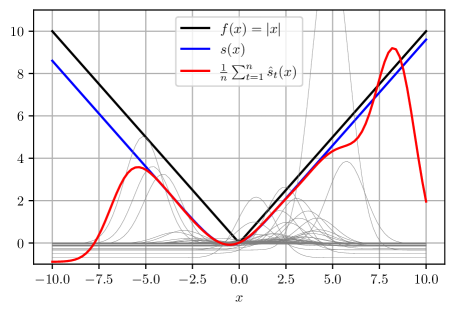
Figure 11.3: The concentration of $\frac{1}{n}\sum_{t=1}^{n}\hat{s}_{t}(x)$ with $f_{t}=f=|\cdot|$ and $n=10^{4}$ and $\mu=\frac{1}{2}$ and $\Sigma=1$ and $\lambda=\frac{1}{2}$. The thin lines correspond to the first one hundred estimated surrogates. The estimate is very close to the real surrogate on an interval around $\mu$ but can be extremely poorly behaved far away, even with $n$ so large. Note also that the estimated surrogate is convex near $\mu$ but not everywhere.

Concentration bounds

We start with a Bernstein-like concentration bound for the sum of the surrogate loss estimators:

Proposition 11.17.

The following hold:

1. Let $x\in\mathbb{R}^{d}$ is a non-random vector such that $x\in K_{\tau}(1/\sqrt{2L})$ almost surely. Then, with probability at least $1-\delta$,

   $$\left|\sum_{t=1}^{\tau}(\hat{s}_{t}(x)-s_{t}(x))\right|\leq 1+\frac{1}{\lambda}\left[\sqrt{LV_{\tau}}+LY_{\max}\right]\,.$$

2. With probability at least $1-\delta$,

   $$\max_{x\in K_{\tau}(1/\sqrt{2dL})}\left|\sum_{t=1}^{\tau}\hat{s}_{t}(x)-s_{t}(x)\right|\leq\frac{1}{\lambda}\sqrt{dLV_{\tau}}+\frac{dLY_{\max}}{\lambda}\,.$$

Note the different radii in (a) and (b) that appear in $K_{\tau}$ and also the extra $\sqrt{d}$ factor that appears in (b). You should view these bounds as a kind of Bernstein inequality with the term involving $Y_{\max}$ the lower-order term and $V_{\tau}=O(\tau)$ with high probability.

Proof.

The single-point bound in (a) follows from a truncation argument followed by a standard application of martingale concentration. The uniform bound in(b) more-or-less follows from a union bound argument in combination with the analysis in part (a).

Proof of part (a)

Let $x\in\mathbb{R}^{d}$ be such that $x\in K_{\tau}(1/\sqrt{2L})$ almost surely and recall that

$$\hat{s}_{t}(x)=\left(1+\frac{R_{t}(x)-1}{\lambda}\right)Y_{t}\,.$$

Let $E_{t}=\{R_{t}(x)\leq 3\exp(4),|Y_{t}|\leq Y_{\max}\}$. By Lemma 11.9,

$$0\leq R_{t}(x)\leq 3\exp\left(4\lambda\left\langle X_{t}-\mu_{t},x-\mu_{t}\right\rangle_{\Sigma_{t}^{-1}}\right)\triangleq 3\exp\left(4Z\right)\,,$$

where the last inequality serves as the definition of $Z$, which under $\mathbb{P}_{t-1}$ has law $\mathcal{N}(0,\lambda^{2}\|x-\mu_{t}\|^{2}_{\Sigma_{t}^{-1}})$. By assumption $\lambda\|x-\mu_{t}\|_{\Sigma_{t}^{-1}}\leq 1/\sqrt{2L}$ and by Theorem B.5,

$$\mathbb{P}(R_{t}(x)\geq 3\exp(4))\leq\mathbb{P}(Z\geq 1)\leq\exp(-L)\,.$$

By assumption, $\mathbb{P}_{t-1}(|Y_{t}|\geq Y_{\max})\leq\exp(-L)$ and hence a union bound shows that $\mathbb{P}(E_{t}^{c})\leq 2\exp(-L)$ and by Cauchy-Schwarz,

$$\left|s_{t}(x)-\mathbb{E}_{t-1}[\bm{1}_{E_{t}}\hat{s}_{t}(x)]\right| \leq\sqrt{\mathbb{E}_{t-1}[\hat{s}_{t}(x)^{2}]\mathbb{P}_{t-1}(E_{t}^{c})}$$

$$\leq\sqrt{2\exp(-L)\mathbb{E}_{t-1}[\hat{s}_{t}(x)^{2}]}$$

$$\leq\frac{1}{n}\,,$$ (11.6)

where in the final inequality we used Lemma 11.14(a) and made sure to choose $L$ large enough. The plan is now to apply Freedman’s inequality to the sequence $(\bm{1}_{E_{t}}\hat{s}_{t}(x))_{t=1}^{\tau}$ for which we need boundedness and a second moment bound. By the definition of $E_{t}$,

$$\left|\bm{1}_{E_{t}}\hat{s}_{t}(x)\right|=\bm{1}_{E_{t}}\left|Y_{t}\left(1+\frac{R_{t}(x)-1}{\lambda}\right)\right|\leq\frac{3\exp(4)Y_{\max}}{\lambda}\,.$$

Furthermore,

$$\mathbb{E}_{t-1}[\bm{1}_{E_{t}}\hat{s}_{t}(x)^{2}] =\mathbb{E}_{t-1}\left[\bm{1}_{E_{t}}Y_{t}^{2}\left(1+\frac{R_{t}(x)-1}{\lambda}\right)^{2}\right]\leq\frac{9\exp(8)}{\lambda^{2}}\mathbb{E}_{t-1}[Y_{t}^{2}]\,.$$

Combining Eq. 11.6 and Eq. 11.7 with Theorem B.7 shows that with probability at least $1-\frac{\delta}{2}$,

$$\left|\sum_{t=1}^{\tau}(\bm{1}_{E_{t}}\hat{s}_{t}(x)-s_{t}(x))\right| \leq 1+\left|\sum_{t=1}^{\tau}\big{(}\bm{1}_{E_{t}}\hat{s}_{t}(x)-\mathbb{E}_{t-1}[\bm{1}_{E_{t}}\hat{s}(x)]\big{)}\right|$$

$$\leq 1+\frac{1}{\lambda}\left[\sqrt{LV_{\tau}}+LY_{\max}\right]\,.$$

Since $\mathbb{P}_{t-1}(E_{t}^{c})\leq 2\exp(-L)\leq\frac{1}{2n\delta}$, a union bound shows that with probability at least $1-\frac{\delta}{2}$,

$$\sum_{t=1}^{\tau}(\hat{s}_{t}(x)-s_{t}(x)) =\sum_{t=1}^{\tau}(\bm{1}_{E_{t}}\hat{s}_{t}(x)-s_{t}(x))$$ (11.7)

Part (a) is now established by combining the above two displays with a union bound.

Proof of part (b)

The argument follows along the same lines as part (a) but now we need an additional covering and Lipschitz argument. Let $\mathcal{C}$ be a finite cover of $K$ such that for all $y\in K$ there exists an $x\in\mathcal{C}$ such that $\left\|x-y\right\|\leq\varepsilon$ with

$$\varepsilon=\left[\max\left(\lambda\sqrt{\Sigma_{\max}^{-1}},\,Cn(1+\sqrt{L})\sqrt{\Sigma_{\max}^{-1}dL}\right)\right]^{-1}\,.$$ (11.8)

By (Vershynin, 2018, Corollary 4.2.13), $\mathcal{C}$ can be chosen so that

$$|\mathcal{C}|\leq\left(\frac{2\operatorname{diam}(K)}{\varepsilon}+1\right)^{d}\,,$$

which means that $\log|\mathcal{C}|\leq dL$. Given a non-empty set $A\subset\mathbb{R}^{d}$ let $d(x,A)=\inf_{y\in A}\left\|x-y\right\|$ and for $x\in\mathcal{C}$ let $\tau_{x}=\min\{t\leq\tau:d(x,K_{t})>\varepsilon\}$. Let $E_{t}$ be the event

$$E_{t}=\left\{\left\|X_{t}-\mu_{t}\right\|_{\Sigma_{t}^{-1}}\leq\sqrt{2dL},|Y_{t}|\leq Y_{\max}\right\}\,.$$

Like in the proof of part (a), $R_{t}(x)\leq 3\exp(4)$ whenever $\left\langle X_{t}-\mu_{t},x-\mu_{t}\right\rangle_{\Sigma_{t}^{-1}}\leq 1$. Furthermore,

$$\max_{x\in K_{t}(1/\sqrt{2dL})}\left\langle X_{t}-\mu_{t},x-\mu_{t}\right\rangle_{\Sigma_{t}^{-1}}\leq\frac{1}{\sqrt{2dL}}\|X_{t}-\mu_{t}\|_{\Sigma_{t}^{-1}}\,.$$

Therefore,

$$\bm{1}_{E_{t}}\max_{x\in K_{t}(1/\sqrt{2dL})}R_{t}(x)\leq 3\exp(4)\,.$$

Repeating the argument in Part (a) along with a union bound over $\mathcal{C}$ shows that

$$\mathbb{P}\left(\max_{x\in\mathcal{C}}\left|\sum_{t=1}^{\tau_{x}}(\hat{s}_{t}(x)-s_{t}(x))\right|\geq 1+\frac{1}{\lambda}\left[\sqrt{dV_{\tau}L}+dLY_{\max}\right]\right)\leq\frac{\delta}{4}\,.$$

Recall the following:

• By assumption: $\mathbb{P}(|Y_{t}|\geq Y_{\max})\leq\exp(-L)$; and

• By Lemma B.3: $\|\|X_{t}-\mu_{t}\|_{\Sigma_{t}^{-1}}\|_{t-1,\psi_{2}}\leq\sqrt{8d/3}$.

Therefore, by a union bound and Lemma B.1, the following all hold with probability at least $1-\delta$:

1. $\max_{x\in\mathcal{C}}\left|\sum_{t=1}^{\tau_{x}}(\hat{s}_{t}(x)-s_{t}(x))\right|\leq 1+\frac{1}{\lambda}\left[\sqrt{dV_{\tau}L}+dLY_{\max}\right]$.

2. $\max_{1\leq t\leq n}|Y_{t}|\leq Y_{\max}$.

3. $\max_{1\leq t\leq n}\left\|X_{t}-\mu_{t}\right\|_{\Sigma_{t}^{-1}}\leq\sqrt{dL}$.

Assume for the remainder that all of (a)-(c) above hold and let $y\in K_{\tau}$. By the construction of $\mathcal{C}$ there exists an $x\in\mathcal{C}$ such that $\left\|x-y\right\|\leq\varepsilon$ and therefore $d(x,K_{\tau})\leq\varepsilon$ and $\tau_{x}=\tau$. Since $y\in K_{\tau}$,

$$\lambda\left\|x-\mu_{t}\right\|_{\Sigma_{t}^{-1}} \leq\lambda\left\|x-y\right\|_{\Sigma_{t}^{-1}}+\lambda\left\|y-\mu_{t}\right\|_{\Sigma_{t}^{-1}}$$

$$\leq\lambda\varepsilon\sqrt{\Sigma_{\max}^{-1}}+\frac{1}{\sqrt{2L}}$$

$$\leq\sqrt{dL}\,,$$

where we used the definition of $K_{\tau}$, the triangle inequality and the definition of $\varepsilon$ in Eq. 11.8 and naive bounding. Next, since $y\in K_{\tau}$,

$$\lambda\left\langle X_{t}-\mu_{t},y-\mu_{t}\right\rangle_{\Sigma_{t}^{-1}} \leq\lambda\left\|X_{t}-\mu_{t}\right\|_{\Sigma_{t}^{-1}}\left\|y-\mu_{t}\right\|_{\Sigma_{t}^{-1}}$$

$$\leq\lambda\sqrt{dL}\left\|y-\mu_{t}\right\|_{\Sigma_{t}^{-1}}$$

$$\leq 1\,,$$

where we used Cauchy-Schwarz, item (c) above and the definition of $K_{\tau}$. Therefore

$$\lambda\left\langle X_{t}-\mu_{t},x-\mu_{t}\right\rangle_{\Sigma_{t}^{-1}} \leq 1+\lambda\left\langle X_{t}-\mu_{t},x-y\right\rangle_{\Sigma_{t}^{-1}}$$

$$\leq 1+\lambda\left\|X_{t}-\mu_{t}\right\|_{\Sigma_{t}^{-1}}\left\|x-y\right\|\sqrt{\left\|\Sigma_{t}^{-1}\right\|}$$

$$\leq 1+\varepsilon\lambda\sqrt{dL\left\|\Sigma_{t}^{-1}\right\|}$$

$$\leq 2\,,$$

where we used the fact that $y\in K_{\tau}\subset K_{t}$ and that $\left\|x-y\right\|\leq\varepsilon$. Combining the above with item (c) provides the conditions for Lemma 11.10, which shows that

$$\left|\hat{s}_{t}(x)-\hat{s}_{t}(y)\right|\leq\operatorname{lip}_{[x,y]}(\hat{s}_{t})\left\|x-y\right\|\leq\varepsilon\operatorname{lip}_{[x,y]}(\hat{s}_{t})\leq\frac{1}{n}\,.$$

where we used item (b) and the definition of $\varepsilon$ in Eq. 11.8. By Proposition 11.2, for any $z\in[x,y]$,

$$\operatorname{lip}_{K}(s_{t})\leq\operatorname{lip}_{K}(f_{t})+\beta\sqrt{d\left\|\Sigma_{t}\right\|}\,.$$

Therefore, using the definition of $\varepsilon$,

$$\left|\sum_{t=1}^{\tau}(\hat{s}_{t}(y)-s_{t}(y))\right| \leq 1+\left|\sum_{t=1}^{\tau}(\hat{s}_{t}(x)-s_{t}(x))\right|$$

$$\leq 2+\frac{1}{\lambda}\left[\sqrt{dV_{\tau}L}+dLY_{\max}\right]\,.$$

∎

More or less the same result holds for the quadratic surrogates estimates.

Proposition 11.18.

Let $r\in[0,1]$. The following hold:

1. Let $x\in\mathbb{R}^{d}$ be a non-random vector such that $x\in K_{\tau}(r)$ almost surely. Then, with probability at least $1-\delta$,

   $$\left|\sum_{t=1}^{\tau}q_{t}(x)-\hat{q}_{t}(x)\right|\leq\frac{rL^{2}}{\lambda}\left[\sqrt{V_{\tau}}+Y_{\max}\right]\,.$$

2. With probability at least $1-\delta$,

   $$\sup_{x\in K_{\tau}(r)}\left|\sum_{t=1}^{\tau}q_{t}(x)-\hat{q}_{t}(x)\right|\leq\frac{rL^{2}}{\lambda}\left[\sqrt{dV_{\tau}}+dY_{\max}\right]\,.$$

Notice that with $r=1$ we see about the same uniform concentration bound for the quadratic surrogate as for the non-quadratic version. The difference is that for smaller $r$ the concentration behaviour is better. Unsurprisingly, in the extreme case that $r=0$, then $q_{t}(\mu_{t})=\hat{q}_{t}(\mu_{t})=0$ almost surely.

Proof.

Let $x\in\mathbb{R}^{d}$ be a non-random vector such that $x\in K_{\tau}(r)$ almost surely. Remember that by definition

$$\hat{q}_{t}(x)=\left\langle g_{t},x-\mu_{t}\right\rangle+\frac{1}{6}\left\|x-\mu_{t}\right\|^{2}_{H_{t}}\,.$$

The first term is

$$\left\langle g_{t},x-\mu_{t}\right\rangle=\frac{R_{t}(\mu_{t})Y_{t}\left\langle x-\mu_{t},X_{t}-\mu_{t}\right\rangle_{\Sigma_{t}^{-1}}}{1-\lambda}$$

The second is

$$\frac{1}{6}\left\|x-\mu_{t}\right\|^{2}_{H_{t}} =\frac{\lambda R_{t}(\mu_{t})Y_{t}}{6(1-\lambda)^{2}}\left[\frac{\left\langle x-\mu_{t},X_{t}-\mu_{t}\right\rangle_{\Sigma_{t}^{-1}}^{2}}{(1-\lambda)^{2}}-\left\|x-\mu_{t}\right\|^{2}_{\Sigma_{t}^{-1}}\right]\,.$$

Note that $\left\langle x-\mu_{t},X_{t}-\mu_{t}\right\rangle_{\Sigma_{t}^{-1}}$ has law under $\mathbb{P}_{t-1}$ of $\mathcal{N}(0,\left\|x-\mu_{t}\right\|_{\Sigma_{t}^{-1}})$. Therefore,

$$\mathbb{P}_{t-1}\left(\left|\left\langle x-\mu_{t},X_{t}-\mu_{t}\right\rangle_{\Sigma_{t}^{-1}}\right|\geq\left\|x-\mu_{t}\right\|_{\Sigma_{t}^{-1}}\sqrt{L}\right)\leq\frac{\delta}{2n}\,.$$

Define an event

$$E_{t}=\left\{|Y_{t}|\leq Y_{\max}\text{ and }\left|\left\langle x-\mu_{t},X_{t}-\mu_{t}\right\rangle_{\Sigma_{t}^{-1}}\right|\leq\left\|x-\mu_{t}\right\|_{\Sigma_{t}^{-1}}\sqrt{L}\right\}\,.$$

By a union bound $\mathbb{P}(\cap_{t=1}^{n}E_{t})\geq 1-2n\exp(-L)$. By Lemma 11.14 and using the fact that $x\in K_{\tau}(r)\subset K_{t}(r)$ for $t\leq\tau$,

$$\mathbb{E}_{t-1}[\hat{q}_{t}(x)\bm{1}_{E_{t}^{c}}]\leq\sqrt{\mathbb{E}_{t-1}[\hat{q}_{t}(x)^{2}]\mathbb{P}_{t-1}(E_{t}^{c})}\leq\frac{1}{n}\,.$$

Furthermore, using the fact that $r\in[0,1]$,

$$\bm{1}_{E_{t}}|\hat{q}_{t}(x)|\leq\frac{rCL|Y_{t}|}{\lambda}\leq\frac{rCLY_{\max}}{\lambda}\,.$$

Therefore, by Theorem B.7, with probability at least $1-\delta$,

$$\left|\sum_{t=1}^{\tau}\left(\hat{q}_{t}(x)-q_{t}(x)\right)\right|\leq\frac{rL^{2}}{\lambda}\left[\sqrt{V_{\tau}}+Y_{\max}\right]\,.$$

Repeating more-or-less the same argument the covering argument in Proposition 11.17 shows that with probability at least $1-\delta$,

$$\sup_{x\in K_{\tau}(r)}\left|\sum_{t=1}^{\tau}\left(\hat{q}_{t}(x)-q_{t}(x)\right)\right|\leq\frac{rL^{2}}{\lambda}\left[\sqrt{dV_{\tau}}+dY_{\max}\right]\,.$$

∎

In the analysis of online Newton step we also make use of concentration of the Hessian estimates of the surrogate, which we now establish.

Proposition 11.19.

Let $\mathscr{S}\subset\mathbb{S}^{d}_{+}$ be the (random) set of positive definite matrices such that $\Sigma_{t}^{-1}\preceq\Sigma^{-1}$ for all $t\leq\tau$ and $S_{t}(x)=\sum_{s=1}^{t}\hat{s}_{t}^{\prime\prime}(x)$ and $\bar{S}_{t}(x)=\sum_{s=1}^{t}s_{t}^{\prime\prime}(x)$. With probability at least $1-\delta$, for all $\Sigma^{-1}\in\mathscr{S}$,

$$\bar{S}_{\tau}(x)-\lambda L^{2}\left[\sqrt{dV_{\tau}}+d^{2}Y_{\max}\right]\Sigma^{-1} \preceq S_{\tau}(x)$$

$$\preceq\bar{S}_{\tau}(x)+\lambda L^{2}\left[\sqrt{dV_{\tau}}+d^{2}Y_{\max}\right]\Sigma^{-1}\,.$$

Proof.

The plan is conceptually the same as the all the previous results. The standard method for proving matrix inequalities is to compare the matrices in all directions, which like in the uniform concentration bounds proven above requires a union bound. Let $\varepsilon>0$ be a constant to be tuned later and $\mathcal{C}_{K}\subset K$ and $\mathcal{C}_{\mathbb{S}}\subset\mathbb{S}^{d-1}_{1}$ be finite sets such that for all $x\in K$ and $u\in\mathbb{S}^{d-1}_{1}$ there exists a $y\in\mathcal{C}_{K}$ and $v\in\mathbb{S}^{d-1}_{1}$ such that $\left\|x-y\right\|\leq\varepsilon$ and $\left\|u-v\right\|\leq\varepsilon$. Let $r=1/\sqrt{2dL}$ and suppose that $y\in K_{\tau}(r)$ and $\left\|x-y\right\|\leq\varepsilon$. Then, for any $t\leq\tau$,

$$\|x-\mu_{t}\|_{\Sigma_{t}^{-1}}\leq\|y-\mu_{t}\|_{\Sigma_{t}^{-1}}+\|x-y\|_{\Sigma_{t}^{-1}}\leq r+\varepsilon\|\Sigma_{t}^{-1}\|^{\frac{1}{2}}\leq 2r\,.$$

Let $x\in\mathbb{R}^{d}$ and $u\in\mathbb{S}^{d-1}_{1}$ and let

$$\tau_{x}=\max\{t\leq\tau:x\in K_{t}(2r)\}\,.$$

Suppose that $y\in K_{\tau}(r)$. Then there exists an $x\in\mathcal{C}_{K}$ such that $\left\|x-y\right\|\leq\varepsilon$ and therefore $x\in K_{\tau}(2r)$ and $\tau_{x}=\tau$. Define the event

$$E_{t}=\left\{|Y_{t}|\leq Y_{\max},\|X_{t}-\mu_{t}\|_{\Sigma_{t}^{-1}}\leq\sqrt{dL}\right\}\,.$$

We will prove in a moment that with probability at least $1-\delta$, $\bigcap_{t=1}^{\tau}E_{t}$ holds and for all $x\in\mathcal{C}_{K}$ and $u\in\mathcal{C}_{\mathbb{S}}$,

$$\sum_{t=1}^{\tau_{x}}\left\|u\right\|^{2}_{\hat{s}^{\prime\prime}(x)}\leq\sum_{t=1}^{\tau_{x}}\left\|u\right\|^{2}_{s^{\prime\prime}(x)}+L^{2}\lambda\left\|u\right\|^{2}_{\Sigma^{-1}}\left[\sqrt{dV_{\tau}}+d^{2}Y_{\max}\right]\,.$$

As we argued above, $\tau_{x}=\tau$ for all $x$ for which there is a $y\in K_{\tau}$ and $\left\|x-y\right\|\leq\varepsilon$. The claim is completed using Lipschitz continuity of all the relevant quantities on $K_{t}$ for all $t\leq\tau$.

Applying Freedman’s

By assumption, $\mathbb{P}_{t-1}(|Y_{t}|\geq Y_{\max})\leq\exp(-L)$ and since $\Sigma_{t}^{-1}(X_{t}-\mu_{t})$ is a standard Gaussian under $\mathbb{P}_{t-1}$ we also have $\mathbb{P}_{t-1}(\|X_{t}-\mu_{t}\|_{\Sigma_{t}^{-1}}\geq\sqrt{dL})\leq\exp(-L)$. Hence, with probability at least $1-\delta/2$, for all $x\in\mathbb{R}^{d}$,

$$\sum_{t=1}^{\tau}\hat{s}^{\prime\prime}(x)=\sum_{t=1}^{n}\bm{1}_{E_{t}}\hat{s}^{\prime\prime}(x)\bm{1}_{E_{t}}\,.$$

At the same time, for any $x\in\mathcal{C}_{K}$,

$$\left|\mathbb{E}\left[\bm{1}_{E_{t}^{c}}\left\|u\right\|^{2}_{\hat{s}^{\prime\prime}(x)}\right]\right| \leq\sqrt{\mathbb{P}(E_{t}^{c})\mathbb{E}_{t-1}\left[\left\|u\right\|^{4}_{\hat{s}^{\prime\prime}(x)}\right]}\leq\frac{1}{n}\,.$$

Therefore, for any $x\in\mathcal{C}_{K}$ and $u\in\mathcal{C}_{\mathbb{S}}$ and $t\leq\tau_{x}$,

$$\left|\mathbb{E}_{t-1}\left[\|u\|^{2}_{H_{t}}\right]-\mathbb{E}_{t-1}\left[\bm{1}_{E_{t}}\|u\|^{2}_{H_{t}}\right]\right|\leq\frac{\Sigma_{\min}^{-1}}{n}\,.$$

We need to bound the various moments of $\left\|u\right\|^{2}_{\hat{s}^{\prime\prime}(x)}$. Let

$$V_{t,x}=\Sigma_{t}^{-1/2}\left(\frac{X_{t}-\lambda x}{1-\lambda}-\mu\right)=\frac{1}{1-\lambda}\Sigma_{t}^{-1/2}\left[X_{t}-\mu+\lambda(\mu-x)\right]\,,$$

which is chosen so that

$$\hat{s}^{\prime\prime}(x)=\frac{\lambda R_{t}(x)Y_{t}}{(1-\lambda)^{2}}\left[\Sigma_{t}^{-1/2}V_{t,x}V_{t,x}^{\top}\Sigma_{t}^{-1/2}-\Sigma_{t}^{-1}\right]\,.$$

Note that

$$\bm{1}_{E_{t}}\left\|V_{t,x}\right\|=\frac{\bm{1}_{E_{t}}}{1-\lambda}\left\|X_{t}-\mu+\lambda(\mu-x)\right\|_{\Sigma_{t}^{-1}}\leq\frac{\sqrt{dL}}{1-\lambda}+2r\leq 4\sqrt{dL}\,.$$

Bounding the absolute magnitude:

$$\bm{1}_{E_{t}}\left\|u\right\|^{2}_{\hat{s}^{\prime\prime}(x)} =\bm{1}_{E_{t}}\frac{\lambda R_{t}(x)Y_{t}}{(1-\lambda)^{2}}u^{\top}\left[\Sigma_{t}^{-1/2}V_{x}V_{x}^{\top}\Sigma_{t}^{-1/2}-\Sigma_{t}^{-1}\right]u$$

$$\leq CLd\lambda Y_{\max}\left\|u\right\|^{2}_{\Sigma_{t}^{-1}}\,,$$

where we used the fact that

$$u^{\top}\Sigma_{t}^{-1/2}V_{x}V_{x}^{\top}\Sigma_{t}^{-1/2}u =\left\langle\Sigma_{t}^{-1/2}u,V_{x}\right\rangle^{2}\leq\left\|u\right\|^{2}_{\Sigma_{t}^{-1}}\left\|V_{x}\right\|^{2}\leq 16dL\left\|u\right\|^{2}_{\Sigma_{t}^{-1}}$$

Bounding the second moment needs a little care to get the dimension-dependence correct. We have

$$\left\langle\Sigma_{t}^{-1/2}u,V_{t,x}\right\rangle\stackrel{{\scriptstyle d}}{{=}}\mathcal{N}\left(\frac{\lambda\left\langle u,\mu-x\right\rangle}{1-\lambda},\frac{1}{(1-\lambda)^{2}}\left\|u\right\|^{2}_{\Sigma_{t}^{-1}}\right)\,.$$

Hence the second moment is bounded by

$$\mathbb{E}\left[\bm{1}_{E_{t}}\left\|u\right\|^{4}_{\hat{s}^{\prime\prime}(x)}\right] \leq\frac{9\exp(8)\lambda^{2}}{(1-\lambda)^{4}}\mathbb{E}_{t-1}\left[\bm{1}_{E_{t}}Y_{t}^{2}\left\langle\Sigma_{t}^{-1/2}u,V_{t,x}\right\rangle^{2}\right]$$

$$\leq L^{2}\lambda^{2}\left\|u\right\|^{4}_{\Sigma_{t}^{-1}}\mathbb{E}_{t-1}[Y_{t}]^{2}\,.$$

Therefore, by Theorem B.7, with probability at least $1-\delta$, for all $u\in\mathcal{C}_{\mathbb{S}}$ and $x\in\mathcal{C}_{K}$ and $\Sigma^{-1}\in\mathscr{S}$,

$$\left|\sum_{t=1}^{\tau_{x}}\left(\left\|u\right\|^{2}_{s^{\prime\prime}(x)}-\left\|u\right\|^{2}_{\hat{s}^{\prime\prime}(x)}\right)\right|\leq\lambda L^{2}\left\|u\right\|^{2}_{\Sigma^{-1}}\left[\sqrt{dV_{\tau}}+d^{2}Y_{\max}\right]\,,$$

which is what we required. ∎

Proposition 11.19 provides a concentration guarantee for the second derivatives of $\hat{s}^{\prime\prime}(x)$ for all $x$ within a certain focus region. The next lemma shows that the accumulation of second derivatives along the sequence $\mu_{1},\ldots,\mu_{\tau}$ is well-concentration, which is used in Chapter 9.

Proposition 11.20.

Let $\mathscr{S}\subset\mathbb{S}^{d}_{+}$ be the (random) set of positive definite matrices such that $\Sigma_{t}^{-1}\preceq\Sigma^{-1}$ for all $t\leq\tau$ and $S_{t}=\sum_{s=1}^{t}\hat{s}_{t}^{\prime\prime}(\mu_{t})$ and $\bar{S}_{t}=\sum_{s=1}^{t}s_{t}^{\prime\prime}(\mu_{t})$. With probability at least $1-\delta$, for all $\Sigma^{-1}\in\mathscr{S}$,

$$\bar{S}_{\tau}-\lambda L^{2}\left[\sqrt{dV_{\tau}}+d^{2}Y_{\max}\right]\Sigma^{-1} \preceq S_{\tau}$$

$$\preceq\bar{S}_{\tau}+\lambda L^{2}\left[\sqrt{dV_{\tau}}+d^{2}Y_{\max}\right]\Sigma^{-1}\,.$$

Proof.

Repeat verbatim the proof of Proposition 11.19 except you no longer need a covering of $K$. Note that controlling the change of measure term is now trivial since $R_{t}(\mu_{t})\leq 3$ holds almost surely. ∎

Proposition 11.21.

The following hold:

1. Suppose that $\max_{1\leq t\leq\tau}\lambda\left\|x-\mu_{t}\right\|_{\Sigma_{t}^{-1}}\leq\frac{1}{\sqrt{2L}}$. Then, for any $u\in\mathbb{R}^{d}$, with probability at least $1-\delta$,

   $$\left|\sum_{t=1}^{\tau}\left\langle\hat{s}^{\prime}(x)-s^{\prime}(x),u\right\rangle\right|\leq\max_{1\leq t\leq\tau}\left\|u\right\|_{\Sigma_{t}^{-1}}L\sqrt{n}\,.$$

2. Let $K_{t}$ be defined as in Proposition 11.17 then with probability at least $1-\delta$ for all $x\in K_{t}$ and $u\in\mathbb{R}^{d}$,

   $$\left|\sum_{t=1}^{\tau}\left\langle\hat{s}^{\prime}(x)-s^{\prime}(x),u\right\rangle\right|\leq\max_{1\leq t\leq\tau}\left\|u\right\|_{\Sigma_{t}^{-1}}L\sqrt{dn}\,.$$

Proof.

For part (a), let $E_{t}=\{|Y_{t}|\leq 1+\sqrt{L},r_{t}(x)\leq 3\exp(4)\}$. As in the proof of Proposition 11.17(a), $\mathbb{P}(E_{t}^{c})\leq 1/P$. Therefore,

$$\left|\mathbb{E}_{t-1}[\bm{1}_{E_{t}^{c}}\left\langle\hat{s}^{\prime}_{t}(x),u\right\rangle]\right|\leq\left\|u\right\|_{\Sigma_{t}^{-1}}\sqrt{\mathbb{P}(E_{t}^{c})\left\|\hat{s}^{\prime}(x)_{t}\right\|^{2}_{\Sigma_{t}}}\leq\frac{1}{n}\left\|u\right\|_{\Sigma_{t}^{-1}}\,.$$

Furthermore,

$$\left\|\bm{1}_{E_{t}}\left\langle\hat{s}_{t}(x),u\right\rangle\right\|_{t-1,\psi_{1}} =\left\|\bm{1}_{E_{t}}r_{t}(x)Y_{t}\left\langle u,\frac{X_{t}-\lambda x}{1-\lambda}-\mu_{t}\right\rangle_{\Sigma_{t}^{-1}}\right\|_{t-1,\psi_{1}}$$

$$\leq 3\exp(4)(1+\sqrt{L})\left\|\left\langle u,\frac{X_{t}-\lambda x}{1-\lambda}-\mu_{t}\right\rangle_{\Sigma_{t}^{-1}}\right\|_{t-1,\psi_{1}}$$

$$\leq\frac{9\exp(4)(1+\sqrt{L})}{1-\lambda}\left\|u\right\|_{\Sigma_{t}^{-1}}\,.$$

Therefore, by Theorem B.8, with probability at least $1-\delta$,

$$\left|\sum_{t=1}^{\tau}\left\langle\hat{s}_{t}^{\prime}(x)-s_{t}^{\prime}(x),u\right\rangle\right|\leq\max_{1\leq t\leq\tau}\left\|u\right\|^{2}_{\Sigma_{t}^{-1}}L\sqrt{n}\,.$$

For part (b), combine the above with the covering argument in Proposition 11.17, covering both $K$ and the set $\{u:\left\|u\right\|\leq 1\}$. ∎

As mentioned several times, $s_{t}$ is convex but $\hat{s}_{t}$ is usually not. The following proposition shows that $\sum_{t=1}^{\tau}\hat{s}_{t}$ is nearly convex on a suitable subset of $K$.

Proposition 11.22.

Let $K_{t}$ be as in Proposition 11.17. Then, with probability at least $1-\delta$, for all $x\in K_{t}$,

$$\sum_{t=1}^{\tau}\hat{s}_{t}^{\prime\prime}(x)\succeq-\lambda\sqrt{dn}L\Sigma^{-1}\,.$$

Proof.

Let $u\in\mathbb{S}^{d-1}_{1}$ and $x\in K$. Then,

$$\left\|\left\|u\right\|^{2}_{\hat{s}^{\prime\prime}(x)}\bm{1}_{E_{t}}\right\|_{t-1,\psi_{1}} \leq\operatorname{C}Y_{\max}\lambda\left\|u\right\|^{2}_{\Sigma_{t}^{-1}}$$

Let $\mathcal{C}_{\mathbb{S}}$ be a cover of $\mathbb{S}^{d-1}_{1}$ so that for all $v\in\mathbb{S}^{d-1}_{1}$ there exists a $u\in\mathcal{C}$ such that $\left\|u-v\right\|\leq\varepsilon$. Similarly, let $\mathcal{C}_{K}$ be a cover of $K$ such that for all $y\in K$ there exists an $x\in\mathcal{C}_{K}$ with $\left\|x-y\right\|\leq\varepsilon$. By a union bound, with probability at least $1-\delta$, for all $x\in\mathcal{C}_{K}$ and $u\in\mathcal{C}_{\mathbb{S}}$,

$$\sum_{t=1}^{\tau}\left\|u\right\|^{2}_{\hat{s}^{\prime\prime}(x)}\geq\alpha\tau-\operatorname{C}Y_{\max}\lambda\left\|u\right\|^{2}_{\Sigma^{-1}}\sqrt{n\log\left(\frac{|\mathcal{C}_{K}||\mathcal{C}_{\mathbb{S}}|}{\delta}\right)}\,.$$

Repeating the naive Lipschitz analysis used in earlier proofs it follows that for all $x\in K_{\tau}$ and $u\in\mathbb{S}^{d-1}_{1}$,

$$\sum_{t=1}^{\tau}\left\|u\right\|^{2}_{\hat{s}^{\prime\prime}(x)} \geq-\operatorname{C}Y_{\max}\lambda\left\|u\right\|^{2}_{\Sigma^{-1}}\sqrt{n\log\left(\frac{|\mathcal{C}_{K}||\mathcal{C}_{\mathbb{S}}|}{\delta}\right)}$$

$$\geq-\lambda\left\|u\right\|^{2}\sqrt{dn}L\Sigma^{-1}\,.$$

Equivalently, $\sum_{t=1}^{\tau}\hat{s}^{\prime\prime}(x)\succeq-\lambda\sqrt{dn}L\Sigma^{-1}$. ∎

11.9  Summary

Let us summarise what has been shown. The surrogate loss function is convex (Lemma 11.1(a)) and optimistic:

$$s(x)\leq f(x)\text{ for all }x\in\mathbb{R}^{d}\,.$$ Lemma 11.1(b)

On the other hand, the surrogate evaluated at $\mu$ is relatively close to $f(\mu)$:

$$\mathbb{E}[f(X)]\leq s(\mu)+\frac{4}{\lambda}\operatorname{tr}(s^{\prime\prime}(\mu)\Sigma)\,.$$ Proposition 11.5

Furthermore, the quadratic surrogate offers the same benefits on the focus region. Specifically, for any $x$ such that $\lambda\left\|x-\mu\right\|_{\Sigma^{-1}}\leq\frac{1}{L}$,

$$\mathbb{E}[f(X)]-f(x)\leq q(\mu)-q(x)+\frac{4}{\lambda}\operatorname{tr}(s^{\prime\prime}(\mu)\Sigma)\,.$$

The effectiveness of the quadratic surrogate arises from the fact that $s$ is nearly quadratic on the focus region. Specifically, provided that $\lambda\left\|x-y\right\|_{\Sigma^{-1}}\leq L^{-1/2}$, then $s^{\prime\prime}(x)\preceq 3s^{\prime\prime}(y)$.

Tail bounds

Regarding the tails of the estimators, the gradient of the surrogate at $\mu$ is well-behaved in the sense that

$$\mathbb{P}\left(\left\|s^{\prime}(\mu)\right\|^{2}_{\Sigma}\geq dLY^{2}\right)\leq\delta\,.$$ Lemma 11.15

Sequential concentration

Recall the notation of the sequential setting explained in Section 11.8. Particularly, that

$$K_{\tau}(r)=\left\{x\in K:\max_{t\leq\tau}\lambda\left\|x-\mu_{t}\right\|_{\Sigma_{t}^{-1}}\leq r\right\}\,.$$

Remember also that $V_{\tau}=\sum_{t=1}^{\tau}\mathbb{E}_{t-1}[Y_{t}^{2}]$ and $Y_{\max}$ is a constant such that $\mathbb{P}(|Y_{t}|\geq Y_{\max})\leq\exp(-L)$. In the sequential setting explained in Section 11.8, the surrogate is well-concentration in the sense that by Theorem 11.17,

1. For $x\in\mathbb{R}^{d}$ such that $x\in K_{\tau}(1/\sqrt{2L})$ almost surely, with probability at least $1-\delta$,

   $$\left|\sum_{t=1}^{\tau}(\hat{s}_{t}(x)-s_{t}(x))\right|\geq 1+\frac{1}{\lambda}\left[\sqrt{LV_{\tau}}+LY_{\max}\right]\,.$$

2. With probability at least $1-\delta$,

   $$\sup_{x\in K_{\tau}(1/\sqrt{2dL})}\left|\sum_{t=1}^{\tau}(\hat{s}_{t}(x)-s_{t}(x))\right|\leq 1+\frac{1}{\lambda}\left[\sqrt{dLV_{\tau}}+dLY_{\max}\right]\,.$$

Similar results hold for the quadratic surrogate. Precisely, by Theorem 11.18,

1. Given any $x\in\mathbb{R}^{d}$ such that $x\in K_{\tau}(r)$ almost surely, with probability at least $1-\delta$,

   $$\left|\sum_{t=1}^{\tau}\hat{q}_{t}(x)-q_{t}(x)\right|\leq\frac{rL^{2}}{\lambda}\left[\sqrt{V_{\tau}}+Y_{\max}\right]\,.$$

2. With probability at least $1-\delta$,

   $$\sup_{x\in K_{\tau}(r)}\left|\sum_{t=1}^{\tau}\hat{q}_{t}(x)-q_{t}(x)\right|\leq\frac{rL^{2}}{\lambda}\left[\sqrt{dV_{\tau}}+dY_{\max}\right]\,.$$

The Hessian estimates are also reasonably well-behaved. Recall that $\mathscr{P}$ is the random set of matrices $\Sigma^{-1}$ such that $\Sigma_{t}^{-1}\preceq\Sigma^{-1}$ for all $t\leq\tau$. Then, with probability at least $1-\delta$ the following holds for all $x\in K_{\tau}(1/\sqrt{2dL})$,

$$\left|\bar{S}_{\tau}(x)-S_{\tau}(x)\right|\preceq\lambda L^{2}\left[\sqrt{dV_{\tau}}+d^{2}Y_{\max}\right]\,,$$

where $S_{\tau}(x)=\sum_{t=1}^{\tau}\hat{s}^{\prime\prime}_{t}(x)$ and $\bar{S}_{\tau}(x)=\sum_{t=1}^{\tau}s^{\prime\prime}_{t}(x)$ and $|A|\preceq B$ means that $A\preceq B$ and $-A\preceq B$ both hold. Under the same conditions, with probability at least $1-\delta$,

$$\left|\bar{S}_{\tau}-S_{\tau}\right|\preceq\lambda L^{2}\left[\sqrt{dV_{\tau}}+d^{2}Y_{\max}\right]\,,$$

where $S_{\tau}=\sum_{t=1}^{\tau}\hat{s}^{\prime\prime}_{t}(\mu_{t})$ and $\bar{S}_{\tau}=\sum_{t=1}^{\tau}s^{\prime\prime}_{t}(\mu_{t})$.

11.10  Notes

1. The optimistic surrogate was introduced in a slightly different form by Bubeck et al. (2017) and in the present form by Lattimore and György (2021a). The quadratic approximation was first used by Lattimore and György (2023), who proved most of the results in this chapter or variants there-of.

2. The parameter $\lambda$ determines the amount of smoothing. The change of measure in Eq. 11.5 blows up as $\lambda\geq 1/d$. Meanwhile, for $\lambda\in(0,1/d)$ there are trade-offs.

   • A large value of $\lambda$ increases the power of the lower bound of Proposition 11.5 showing that $s$ is not too far below $f$.

   • A large value of $\lambda$ decreases the focus region on which the quadratic surrogate is close to the non-quadratic surrogate and where the concentration properties of the estimators are well-behaved.

Chapter 12  Outlook

The tool-chest for convex bandits and zeroth-order optimisation has been steadily growing in recent decades. Nevertheless, there are many interesting open questions both theoretical and practical. The only purpose of this short chapter is to highlight some of the most important (in the author’s view, of course) open problems. We ignore all logarithmic factors here. The time will one day arrive when the only dregs left will be chasing logarithmic factors, but it is not here yet.

1. The most fundamental problem is to understand the minimax regret for $\mathscr{F}_{\tiny{\texttt{b}}}$. The lower bound is $d\sqrt{n}$ and the upper bound is $d^{2.5}\sqrt{n}$ with the latter bound obtained by non-constructive means. In light of the many positive results for slightly more constrained classes a reasonable conjecture is that the minimax regret is $d^{1.5}\sqrt{n}$. That no one could yet prove this is a lower bound, however, suggests that $d\sqrt{n}$ may be the minimax rate. At the moment it seems we need to push hard on both ends.

2. From a practical perspective the situation is still relatively dire for $d>1$. The algorithms that are simple and efficient to implement have slow convergence rates without smoothness and strong convexity. Algorithms with fast convergence rates have awkward assumptions. For example, Online Newton step learns fast for $\mathscr{F}_{\tiny{\texttt{b}},\tiny{\texttt{u}}}^{\tiny{\texttt{s}}}$ and is difficult to tune. Is there a simple algorithm that works well in practice without too much tuning and obtains the fast rate?

3. Algorithms that manage $O(\sqrt{n})$ regret without smoothness and strong convexity all estimate some kind of curvature or use continuous exponential weights. In particular, they use $\Omega(d^{2})$ memory. Can you prove this is necessary?

4. In the stochastic setting the range of the losses should appear as a second-order term in the regret. Sadly, the only algorithm for which this is true is the bisection method from Chapter 4, which only works when $d=1$. This weakness should be rectified somehow.

5. More adaptive algorithms are needed. We have seen a plethora of results for this algorithm or that with such-and-such assumptions. But what if you don’t know what class the losses lie in. Can you adapt? What is the price? Very few works consider this or have serious limitations. A good place to start is the paper by Luo et al. (2022).

6. There is scope to refine the algorithms and analysis in this text to the non-convex case. Of course, proving bounds relative to a stationary point rather than a global minimum. Someone should push this program through.

7. We mentioned that the center of gravity method could potentially replace the ellipsoid method using the tools in Chapter 10.

8. Almost all of the properties we proved for the optimistic surrogate relied on Gaussianity of the exploration distribution. Two properties that do not rely on this, however, are optimism and convexity. This leaves hope that something may be possible using an exponential weights distribution rather than a Gaussian and this may interact better with the geometry of the constraint set. This seems to have been the original plan of Bubeck et al. (2017) before they resorted to approximating exponential weights distributions by Gaussians. Perhaps you can make it work.

9. Suggala et al. (2021) and Bubeck et al. (2017) both handle adversarial problems by some sort of test to see if the adversary is moving the minimum and proving that if this occurs, then the regret must be negative and it is safe to restart the algorithm. One might wonder if there is some black box procedure to implement this program so that any algorithm designed for the stochastic setting can be used in the adversarial setting.

10. It would be fascinating to gain a better understanding of Algorithm 16. What loss estimators does it use? Maybe you can somehow implement this algorithm when $d=1$ or derive analytically what the estimators look like for special cases.

Appendix A Miscellaneous

A.1  Identities

Lemma A.1.

$\operatorname{vol}(\mathbb{S}^{d-1}_{r})=\frac{d}{r}\operatorname{vol}(\mathbb{B}^{d}_{r})$.

Proposition A.2.

Suppose that $W$ has law $\mathcal{N}(\bm{0},\Sigma)$. Then,

1. $\mathbb{E}[\left\|W\right\|^{2}]=\operatorname{tr}(\Sigma)$.

2. $\mathbb{E}[\left\|W\right\|^{4}]=\operatorname{tr}(\Sigma)^{2}+2\operatorname{tr}(\Sigma^{2})$.

3. $\mathbb{E}[\exp(\left\langle W,a\right\rangle)]=\exp\left(\frac{1}{2}\left\|a\right\|^{2}_{\Sigma}\right)$.

A.2  Technical inequalities

Lemma A.3.

Suppose that $A,B,C>0$. Then,

$$\min_{\eta>0,r>0}\left(\frac{A}{\eta}+\frac{\eta B}{r^{2}}+rC\right)=\sqrt{8}(AB)^{\frac{1}{4}}C^{\frac{1}{2}}$$

with the minimising values of $\eta$ and $r$ being

$$\eta =\left(\frac{2}{C}\right)^{\frac{1}{2}}A^{\frac{3}{4}}B^{-\frac{1}{4}} r =\left(\frac{2}{C}\right)^{\frac{1}{2}}(AB)^{\frac{1}{4}}\,.$$

Lemma A.4.

Suppose that $A,B,C>0$. Then,

$$\min_{\eta>0,r>0}\left(\frac{A}{\eta}+\frac{\eta B}{r^{2}}+r^{2}C\right)=3(ABC)^{\frac{1}{3}}\,.$$

with the minimising values of $\eta$ and $r$ being

$$\eta =A^{\frac{2}{3}}B^{-\frac{1}{3}}C^{-\frac{1}{3}} r^{2} =A^{\frac{1}{3}}B^{\frac{1}{3}}C^{-\frac{2}{3}}\,.$$

Lemma A.5.

Suppose that $u,v\in\mathbb{S}^{d-1}_{1}$ and $A\in\mathbb{R}^{d\times d}$ is symmetric. Then,

$$u^{\top}Au\leq v^{\top}Av+2\left\|u-v\right\|\left\|A\right\|\,.$$

Proof.

Using symmetry of $A$ and Cauchy-Schwarz and the definition of the spectral norm,

$$u^{\top}Au-v^{\top}Av =(u-v)^{\top}A(u+v)\leq\left\|u-v\right\|\left\|A(u+v)\right\|\leq 2\left\|u-v\right\|\left\|A\right\|\,.\qed$$

Lemma A.6.

Suppose that $A$ is positive definite and $A\preceq\bm{1}$. Then $\operatorname{tr}(A)\leq 2\log\det(\mathds{1}+A)$.

Proof.

Use the fact that the trace is the sum of the eigenvalues and the determinant is the product and that $x\leq 2\log(1+x)$ for $x\in[0,1]$. ∎

Lemma A.7.

Suppose that $X$ has law $\mathcal{N}(\mu,\Sigma)$ and $\mathbb{P}(X\notin K)\leq\frac{1}{4}$. Then $\left\|\Sigma\right\|^{1/2}\leq\frac{3}{2}\operatorname{diam}(K)$.

Proof.

Suppose on the contrary that $\frac{1}{3}\left\|\Sigma\right\|^{1/2}>\frac{1}{2}\operatorname{diam}(K)$. Then,

$$\frac{1}{2} \geq 2\mathbb{P}(X\notin K)$$

$$\geq\mathbb{P}(X\notin K\text{ or }-X\notin K)$$ Union bound

$$\geq\mathbb{P}\left(\left\|X-\mu\right\|>\frac{\operatorname{diam}(K)}{2}\right)$$ Definition of diameter

$$>\mathbb{P}\left(\left\|X-\mu\right\|>\frac{1}{3}\left\|\Sigma\right\|^{1/2}\right)$$ Assumption

$$\geq\frac{1}{2}\,.$$ Gaussian integral

∎

Appendix B Concentration

B.1  Orlicz norms

Given a random variable $X$ and $k\in\{1,2\}$ let

$$\left\|X\right\|_{\psi_{k}}=\inf\left\{t>0:\mathbb{E}\left[\exp\left(|X/t|^{k}\right)\right]\leq 2\right\}\,.$$

The random variable $X$ is called subgaussian if $\left\|X\right\|_{\psi_{2}}<\infty$ and subexponential if $\left\|X\right\|_{\psi_{1}}<\infty$. As explained in detail by Vershynin [2018], this definition is equivalent except for universal constants to the definitions based on moments or the moment generating function, which appear, for example, in the book by Boucheron et al. [2013].

Lemma B.1.

Given any random variable $X$ and $t>0$,

1. $\mathbb{P}(|X|\geq t)\leq 2\exp\left(-\frac{t}{\left\|X\right\|_{\psi_{1}}}\right)$.

2. $\mathbb{P}(|X|\geq t)\leq 2\exp\left(-\frac{t^{2}}{\left\|X\right\|^{2}_{\psi_{2}}}\right)$.

Proof.

Both results follow from a standard method. For (a),

$$\mathbb{P}(|X|\geq t) =\mathbb{P}\left(\exp\left(\frac{X}{\left\|X\right\|_{\psi_{1}}}\right)\geq\exp\left(\frac{t}{\left\|X\right\|_{\psi_{1}}}\right)\right)$$

$$\leq 2\exp\left(-\frac{t}{\left\|X\right\|_{\psi_{1}}}\right)\,.$$ Markov’s inequality

Part (b) is left as an exercise. ∎

Lemma B.2.

Given any random variable $X$ and $k\geq 1$, $\mathbb{E}[|X|^{k}]\leq\Gamma(1+k)\left\|X\right\|_{\psi_{1}}^{k}$ where $\Gamma(1+k)$ is the Gamma function.

Proof.

Since $|X|$ is non-negative,

$$\mathbb{E}[|X|^{k}] =\int_{0}^{\infty}\mathbb{P}(|X|^{k}\geq t)\operatorname{d}\!t$$

$$=\int_{0}^{\infty}\mathbb{P}(|X|\geq t^{1/k})\operatorname{d}\!t$$

$$\leq\int_{0}^{\infty}2\exp\left(-\frac{t^{1/k}}{\left\|X\right\|_{\psi_{1}}}\right)\operatorname{d}\!t$$

$$=2\Gamma(1+k)\left\|X\right\|_{\psi_{1}}^{k}\,.\qed$$

Lemma B.3 (Lattimore and György 2023).

Suppose that $W$ is a standard Gaussian random variable in $\mathbb{R}^{d}$. Then:

1. $\left\|\left\langle x,W\right\rangle\right\|_{\psi_{2}}=2\sqrt{2/3}\left\|x\right\|$.

2. $\left\|\operatorname{tr}(AWW^{\top})\right\|_{\psi_{1}}\leq 3\operatorname{tr}(A)$.

3. $\left\|\left\|W\right\|^{2}\right\|_{\psi_{1}}\leq 8d/3$.

4. $\left\|\left\|WW^{\top}-\mathds{1}\right\|\right\|_{\psi_{1}}\leq 5d$.

Lemma B.4.

Suppose that $|X|\leq B$. Then $\left\|X\right\|_{\psi_{2}}\leq\frac{B}{\sqrt{\log(2)}}$.

B.2  Concentration

The following are classical:

Theorem B.5.

Suppose that $X$ has law $\mathcal{N}(0,1)$. Then, for any $x\geq 0$,

$$\mathbb{P}(X\geq x)\leq\frac{1}{2}\exp\left(-\frac{x^{2}}{2}\right)\,.$$

Theorem B.6.

Let $X_{1},\ldots,X_{n}$ be a sequence of independent random variables. Then, for any $\delta\in(0,1)$,

$$\mathbb{P}\left(\sum_{t=1}^{n}\left(X_{t}-\mathbb{E}[X_{t}]\right)\geq\sigma\sqrt{n\log(2/\delta)}\right)\leq\delta\,,$$

where $\sigma=\max\{\left\|X_{t}\right\|_{\psi_{2}}:1\leq t\leq n\}$.

Theorem B.7 (Freedman’s inequality).

Let $X_{1},\ldots,X_{n}$ be a sequence of random variables adapted to filtration $(\mathscr{F}_{t})$ and $\tau$ be a stopping time with respect to $(\mathscr{F}_{t})_{t=1}^{n}$ with $\tau\leq n$ almost surely. Let $\mathbb{E}_{t}[\cdot]=\mathbb{E}[\cdot|\mathscr{F}_{t}]$ and $|X_{t}|\leq B$ almost surely for all $t\leq\tau$. Then, with probability at least $1-\delta$,

$$\left|\sum_{t=1}^{\tau}X_{t}\left(X_{t}-\mathbb{E}_{t-1}[X_{t}]\right)\right|\leq C\left[\sqrt{V_{\tau}\log\left(\frac{\log(1+|V_{\tau}|)}{\delta}\right)}+B\log\left(\frac{1}{\delta}\right)\right]\,,$$

where $V_{\tau}=\sum_{t=1}^{\tau}\mathbb{E}_{t-1}[(X_{t}-\mathbb{E}_{t-1}[X_{t}])^{2}$ is the sum of the predictable variations and $C>0$ is a sufficiently large absolute constant.

We need a simple martingale-style concentration inequality. Obviously these things are ten-a-penny but as usual this particular one is apparently not in the literature.

Theorem B.8.

Let $X_{1},\ldots,X_{n}$ be a sequence of random variables adapted to filtration $(\mathscr{F}_{t})_{t=1}^{n}$ and $\tau$ be a stopping time with respect to $(\mathscr{F}_{t})_{t=1}^{n}$ with $\tau\leq n$ almost surely. Let $\mathbb{E}_{t}[\cdot]=\mathbb{E}[\cdot|\mathscr{F}_{t}]$. Then

$$\mathbb{P}\left(\left|\sum_{t=1}^{\tau}\left(X_{t}-\mathbb{E}_{t-1}[X_{t}]\right)\right|\leq C\sigma\sqrt{n\log\left(\frac{1+|\log(\sigma)|}{\delta}\right)}\right)\geq 1-\delta\,.$$

where $C>0$ is a universal constant and $\sigma=\max_{1\leq t\leq\tau}\left\|X_{t}\right\|_{t-1,\psi_{1}}$ with

$$\left\|X_{t}\right\|_{t-1,\psi_{1}}=\inf\{\theta>0:\mathbb{E}[\exp(|X_{t}/\theta|)|\mathscr{F}_{t-1}]\leq 2\}$$

the subexponential Orlicz norm with respect to $\mathbb{P}(\cdot|\mathscr{F}_{t-1})$.

Proof.

Throughout the proof we let $c,C>0$ be suitably small/large universal constants that may change from one expression to the next. Given $\varepsilon>0$ let

$$\tau_{\varepsilon}=\min\{t\leq\tau:\left\|X_{t+1}\right\|_{t,\psi_{1}}>\varepsilon\}\,,$$

where the minimum of the empty set is defined to be $\tau$. Note that $\left\|X_{t+1}\right\|_{t,\psi_{1}}$ is $\mathscr{F}_{t}$-measurable so $\tau_{\varepsilon}$ is a stopping time with respect to the filtration $(\mathscr{F}_{t})_{t=1}^{n}$.

Step 1: Point-wise bounds

Given any $\lambda>0$. Suppose that $|\lambda|\leq\frac{c}{\varepsilon}$ with $c>0$ a suitably small universal constant. Then, following the proof of [Vershynin, 2018, Theorem 2.8.1],

$$\mathbb{E}_{t-1}[\exp(\lambda X_{t})]\leq\exp\left(C\lambda^{2}\varepsilon^{2}\right)\,.$$

Therefore

$$\mathbb{E}\left[\exp\left(\lambda\sum_{t=1}^{\tau_{\varepsilon}}X_{t}-C\tau_{\varepsilon}\lambda^{2}\varepsilon^{2}\right)\right]\leq 1\,.$$

Hence, By Markov’s inequality,

$$\mathbb{P}\left(\exp\left(\lambda\sum_{t=1}^{\tau_{\varepsilon}}X_{t}-C\tau_{\varepsilon}\lambda^{2}\varepsilon^{2}\right)\leq\frac{1}{\delta}\right)\geq 1-\delta\,.$$

And on this event

$$\sum_{t=1}^{\tau_{\varepsilon}}X_{t}\leq C\tau_{\varepsilon}\lambda\varepsilon^{2}+\frac{1}{\lambda}\log\left(1/\delta\right)\,.$$

Choosing $\lambda=\min\left(\frac{1}{\varepsilon}\sqrt{\frac{\log(1/\delta)}{n}},\frac{c}{\varepsilon}\right)$ shows that

$$\sum_{t=1}^{\tau_{\varepsilon}}X_{t}\leq C\varepsilon\left[\sqrt{n\log(1/\delta)}+\log(1/\delta)\right]\,.$$

Step 2: Union bounds

Let $\mathcal{E}=\{2^{-k}:k\in\mathbb{Z}\}$. Note that $\sum_{k=-\infty}^{\infty}\frac{1}{4k(k+1)}=1$. Therefore, by the previous step, with probability at least $1-\delta$, for all $\varepsilon\in\mathcal{E}$,

$$\sum_{t=1}^{\tau_{\varepsilon}}X_{t}\leq C\varepsilon\left[\sqrt{n\log\left(\frac{k+1}{\delta}\right)}+\log\left(\frac{k+1}{\delta}\right)\right]\,.$$

Let

$$\varepsilon=\min\left\{\theta\in\mathcal{E}:\theta\geq\sigma\right\}\,.$$

Then $\tau_{\varepsilon}=\tau$ and with probability at least $1-\delta$,

$$\sum_{t=1}^{\tau}X_{t} \leq C\sigma\left[\sqrt{n\log\left(\frac{1+|\log(\sigma)|}{\delta}\right)}+\log\left(\frac{k+1}{\delta}\right)\right]\,.\qed$$

Appendix C Computation

Our algorithms need to perform a number of operations on convex sets. For example, Algorithm 7 needs to implement projections while Algorithm 8 needs to compute a self-concordant barrier on $K$. The computation complexity of these operations depends on how $K$ is represented. Convex sets can be represented in many ways but some typical choices are:

1. As a polytope: $K=\{x:Ax\leq b\}$.

2. As the convex hull of a point cloud: $K=\operatorname{conv}(P)$ with $P\subset\mathbb{R}^{d}$.

3. Via a separation oracle, which is an oracle that accepts a point $x\in\mathbb{R}^{d}$ and (1) if $x\in K$, then it says so or (2) if $x$ is not in $K$ then it returns a nonzero vector $\eta$ such that $K\subset\{y:\left\langle y-x,\eta\right\rangle\leq 0\}$.

4. Via a linear optimisation oracle, which is an oracle that accepts as input some vector $v\in\mathbb{R}^{d}$ and outputs a point $x\in\operatornamewithlimits{arg\,min}_{y\in K}\left\langle y,v\right\rangle$.

5. Via a membership oracle, which is an oracle that accepts a point $x\in\mathbb{R}^{d}$ and returns $\bm{1}_{K}(x)$.

Membership to separation

A membership oracle is clearly weaker than a separation oracle but there is an oracle polynomial time reduction from a membership oracle to a separation oracle provided that $K$ is centered and well rounded, which means there is a known $x\in\mathbb{R}^{d}$ and $0<r<R<\infty$ such that $x+\mathbb{B}^{d}_{r}\subset K\subset\mathbb{B}^{d}_{R}$ [Grötschel et al., 2012, Theorem 3.2.4].

Convex hull of point-cloud to separation

Given a point cloud $P=\{x_{1},\ldots,x_{m}\}$, the membership oracle component of the separation oracle corresponds to feasibility of the linear program: $x=\sum_{k=1}^{m}p_{k}x_{k}$ with $p\in\Delta_{m}$. Suppose that $x$ is not in $K$, then a separating vector can also be found via linear feasibility. For example, finding an $\eta$ such that $\left\|\eta\right\|_{\infty}\leq 1$ and $\left\langle x_{k}-x,\eta\right\rangle\leq 0$ for all $k=1,\ldots,m$. By contrast, when $K=\operatorname{conv}(P)$, then a linear optimisation oracle can be implemented trivially in $O(m)$ time.

Projection

Euclidean projection onto a polytope is most efficiently implemented using Newton’s method, which typically converges extremely fast. If you only have a separation oracle, then you may have to resort to the ellipsoid method. If you have a linear optimisation oracle you could use Frank–Wolfe [Frank and Wolfe, 1956].

Self-concordant barriers

When $K=\{x:Ax\leq b\}$ is a polytope and $A=(a_{1},\ldots,a_{m})^{\top}$ has $m$ rows, then $R(x)=-\sum_{k=1}^{m}\log(\left\langle a_{k},x\right\rangle-b_{k})$ is an $m$-self-concordant barrier on $K$. The logarithmic barrier is not an intrinsically defined barrier in the sense that it depends on the representation. Furthermore, when $m$ is very large it may be a very inefficient barrier. The volumetric barrier is another simple to implement barrier that improves the self-concordance to $O(d\sqrt{m})$ [Vaidya, 1996]. The Lee–Sidford barrier improves the self-concordance parameter to $O(d\log(m))$ while remaining practical. In general there always exists a $\vartheta$-self-concordant barrier with $\vartheta\leq d$ [Bubeck and Eldan, 2014, Chewi, 2023] but sadly it is not practically computable. You can find many more examples of $\vartheta$-self-concordant barriers in the notes by Nemirovski [1996].

C.1  Approximating minimum volume enclosing ellipsoids

The material here summarises results by [Grötschel et al., 2012, Chapter 4]. The objective is find a computationally efficient algorithm for approximating $\operatorname{\textsc{mvee}}(K)$ for convex bodies $K$ represented as polytopes via inequality constraints or a separation oracle. Finding the exact minimum volume enclosing or enclosed ellipsoid is computationally hard even when $K$ is represented by a polytope but there do exist efficient approximations.

• When $K=\{x:Ax\leq b\}$, then there exists a polynomial time algorithm for finding an ellipsoid $E=E(x,V)$ such that $E(x,\frac{1}{4d^{2}}V)\subset K\subset E(x,V)$.

• When $K$ is given by a separation oracle, then there exists a polynomial time algorithm for finding an ellipsoid $E=E(x,V)$ such that $E(x,\frac{1}{4d^{3}}V)\subset K\subset E(x,V)$.

Remark C.1.

Approximate minimum/maximum volume enclosing/enclosed ellipsoids can be used to find near-maximal $r$ such that $x+\mathbb{B}^{d}_{r}\subset K$ for some $x$. Define

$$r_{\star}=\max\{r:x+\mathbb{B}^{d}_{r}\subset K,x\in K\}\,.$$

Given an ellipsoid $E=E(x,A)$ such that $E(x,\alpha A)\subset K\subset E(x,A)$ and let $\lambda$ be the smallest eigenvalue of $A$ and $r=\alpha\sqrt{\lambda}$. Then $x+\mathbb{B}^{d}_{r}\subset K$ and $r\leq r_{\star}\leq r/\alpha$.

Polytopes

Let $K=\{x:Ax\leq b\}$ be a polytope with $m$ constraints so that $A\in\mathbb{R}^{m\times d}$. The idea is to use the ellipsoid method. We describe a procedure that accepts the parameters of $K$ and an ellipsoid $E=E(x,V)$ with $K\subset E$ as inputs and either

1. declares that $E(x,r^{2}V)\subset K$ where $r=\frac{1}{2d}$ or;

2. returns a new ellipsoid $E(y,W)\supset K$ with

   $$\operatorname{vol}(E(y,W)\leq\exp\left(-\frac{1}{20d}\right)\operatorname{vol}(E(x,V))\,.$$ (C.1)

Start with some ellipsoid $E_{1}\supset K$ and iterate the procedure until it declares some ellipsoid is contained in $K$. Since the volume reduces by a constant factor in every iteration, the number of iterations needed before the process ends is at most

$$O\left(d\log\left(\frac{\operatorname{vol}(E_{1})}{\operatorname{vol}(K)}\right)\right)\,.$$

The procedure is fairly straightforward:

1. Let $a_{k}$ be the $k$th row of $A$ and check that $E(x,r^{2}V)\subset K$ if and only if for all $1\leq k\leq m$,

   $$y_{k}=x+r\frac{Va_{k}}{\left\|a_{k}\right\|_{V}}\in K\,.$$

2. Declare that $E(x,r^{2}V)\subset K$ if $y_{k}\in K$ for all $1\leq k\leq m$.

3. Otherwise, let $k$ be such that $y_{k}\notin K$ so that

   $$K\subset\{y:\left\langle y-y_{k},a_{k}\right\rangle\leq 0\}\triangleq H\,.$$

4. Let $E(y,W)=\operatorname{\textsc{mvee}}(E(x,V)\cap H\})$ and note that

   $$\left|\frac{\left\langle a_{k},x\right\rangle-\left\langle a_{k},y_{k}\right\rangle}{\left\|a_{k}\right\|_{V}}\right|=r=\frac{1}{2d}\,.$$

   Therefore by Lemma 10.3, $\operatorname{vol}(E(y,W))\leq\exp\left(-\frac{1}{20d}\right)\operatorname{vol}(E(x,V))$.

Separation oracle

When $K$ is a separation oracle there is no straightforward procedure for checking whether or not $E(x,r^{2}V)\subset K$. What we have instead is a procedure that accepts $K$ and $E$ as inputs and does one of two things:

1. Declares that $E(x,\frac{r^{2}}{d}V)\subset K$ where $r=\frac{1}{2d}$; or

2. Returns a new ellipsoid $E(y,W)\subset K$ such that Eq. C.1 holds.

As for polytopes the procedure is simple:

1. Let $v_{1},\ldots,v_{d}$ be the eigenvectors of $V$ and $\lambda_{1},\ldots,\lambda_{d}$ the corresponding eigenvalues and $y_{k}=x+r\lambda_{k}^{1/2}v_{k}$.

2. Query the separation oracle on $y_{1},\ldots,y_{d}$. Suppose that $y_{k}\notin K$, then let $H$ be the half-space returned by the separation oracle and return $E(y,W)=\operatorname{\textsc{mvee}}(E(x,V)\cap H)$.

3. Otherwise $y_{1},\ldots,y_{d}\subset K$ and hence

   $$E(x,\textstyle{\frac{r^{2}}{d}}V)\subset\operatorname{conv}(y_{1},\ldots,y_{d})\subset K\,.$$

Like for polytopes, the procedure is guaranteed to end after at most

$$O\left(d\log\left(\frac{\operatorname{vol}(E_{1})}{\operatorname{vol}(K)}\right)\right)$$

iterations.

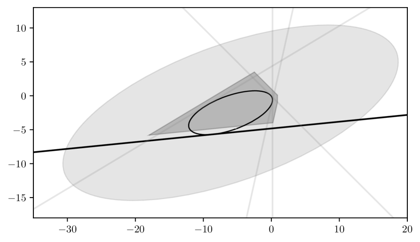
Figure C.1: The construction used for finding a near-optimal minimum volume enclosed ellipsoid for a polytope. The outer ellipsoid is $E(x,V)$ and contains the polytope. The inner ellipsoid is $E(x,\frac{1}{r^{2}}V)$. The procedure tests if the supporting hyperplanes to $E(x,\frac{1}{r^{2}}V)$ are separating hyperplanes for each normal defining the polytope. If none are, then $E(x,\frac{1}{r^{2}}V)$ is contained in $K$ and otherwise you can continue the process with $\operatorname{\textsc{mvee}}(E\cap H)$ for the separating hyperplane found.

References

- Abernethy et al. [2008] J. D. Abernethy, E. Hazan, and A. Rakhlin. Competing in the dark: An efficient algorithm for bandit linear optimization. In Proceedings of the 21st Conference on Learning Theory, pages 263–274. Omnipress, 2008.
- Agarwal et al. [2010] A. Agarwal, O. Dekel, and L. Xiao. Optimal algorithms for online convex optimization with multi-point bandit feedback. In Conference on Learning Theory, pages 28–40. Citeseer, 2010.
- Agarwal et al. [2011] A. Agarwal, D. P. Foster, D. J. Hsu, S. M. Kakade, and A. Rakhlin. Stochastic convex optimization with bandit feedback. In Advances in Neural Information Processing Systems, pages 1035–1043. Curran Associates, Inc., 2011.
- Agarwal et al. [2013] A. Agarwal, D. P. Foster, D. Hsu, S. M. Kakade, and A. Rakhlin. Stochastic convex optimization with bandit feedback. SIAM Journal on Optimization, 23(1):213–240, 2013.
- Artstein-Avidan et al. [2015] S. Artstein-Avidan, A. Giannopoulos, and V. D. Milman. Asymptotic geometric analysis, Part I, volume 202. American Mathematical Soc., 2015.
- Bach and Perchet [2016] F. Bach and V. Perchet. Highly-smooth zero-th order online optimization. In Conference on Learning Theory, pages 257–283. PMLR, 2016.
- Balasubramanian and Ghadimi [2022] K. Balasubramanian and S. Ghadimi. Zeroth-order nonconvex stochastic optimization: Handling constraints, high dimensionality, and saddle points. Foundations of Computational Mathematics, pages 1–42, 2022.
- Belloni et al. [2015] A. Belloni, T. Liang, H. Narayanan, and A. Rakhlin. Escaping the local minima via simulated annealing: Optimization of approximately convex functions. In Conference on Learning Theory, pages 240–265, 2015.
- Boucheron et al. [2013] S. Boucheron, G. Lugosi, and P. Massart. Concentration inequalities: A nonasymptotic theory of independence. OUP Oxford, 2013.
- Bubeck and Cesa-Bianchi [2012] S. Bubeck and N. Cesa-Bianchi. Regret analysis of stochastic and nonstochastic multi-armed bandit problems. Foundations and Trends in Machine Learning, 5(1):1–122, 2012.
- Bubeck and Eldan [2014] S. Bubeck and R. Eldan. The entropic barrier: a simple and optimal universal self-concordant barrier. arXiv preprint arXiv:1412.1587, 2014.
- Bubeck and Eldan [2018] S. Bubeck and R. Eldan. Exploratory distributions for convex functions. Mathematical Statistics and Learning, 1(1):73–100, 2018.
- Bubeck et al. [2012] S. Bubeck, N. Cesa-Bianchi, and S. Kakade. Towards minimax policies for online linear optimization with bandit feedback. In Proceedings of the 25th Conference on Learning Theory, pages 41–1. Microtome, 2012.
- Bubeck et al. [2015] S. Bubeck, O. Dekel, T. Koren, and Y. Peres. Bandit convex optimization: regret in one dimension. In Proceedings of the 28th Conference on Learning Theory, pages 266–278, Paris, France, 2015. JMLR.org.
- Bubeck et al. [2017] S. Bubeck, Y.T. Lee, and R. Eldan. Kernel-based methods for bandit convex optimization. In Proceedings of the 49th Annual ACM SIGACT Symposium on Theory of Computing, STOC 2017, pages 72–85, New York, NY, USA, 2017. ACM. ISBN 978-1-4503-4528-6.
- Bubeck et al. [2018] S. Bubeck, R. Eldan, and J. Lehec. Sampling from a log-concave distribution with projected langevin monte carlo. Discrete & Computational Geometry, Apr 2018.
- Cesa-Bianchi and Lugosi [2006] N. Cesa-Bianchi and G. Lugosi. Prediction, learning, and games. Cambridge University Press, 2006.
- Cheshire et al. [2020] J. Cheshire, P. Ménard, and A. Carpentier. The influence of shape constraints on the thresholding bandit problem. In Conference on Learning Theory, pages 1228–1275. PMLR, 2020.
- Chewi [2023] S. Chewi. The entropic barrier is n-self-concordant. In Geometric Aspects of Functional Analysis: Israel Seminar (GAFA) 2020-2022, pages 209–222. Springer, 2023.
- Conn et al. [2009] A. Conn, K. Scheinberg, and L. Vicente. Introduction to derivative-free optimization. SIAM, 2009.
- Dani et al. [2008] V. Dani, T. P. Hayes, and S. M. Kakade. Stochastic linear optimization under bandit feedback. In Proceedings of the 21st Conference on Learning Theory, pages 355–366, 2008.
- Drori [2018] Y. Drori. On the properties of convex functions over open sets. arXiv preprint arXiv:1812.02419, 2018.
- Duchi et al. [2015] J. Duchi, M. Jordan, M. Wainwright, and A. Wibisono. Optimal rates for zero-order convex optimization: The power of two function evaluations. IEEE Transactions on Information Theory, 61(5):2788–2806, 2015.
- Flaxman et al. [2005] A Flaxman, A Kalai, and HB McMahan. Online convex optimization in the bandit setting: Gradient descent without a gradient. In SODA’05: Proceedings of the sixteenth annual ACM-SIAM symposium on Discrete algorithms, pages 385–394, 2005.
- Foster et al. [2021] D. J. Foster, S. Kakade, J. Qian, and A. Rakhlin. The statistical complexity of interactive decision making. arXiv preprint arXiv:2112.13487, 2021.
- Foster et al. [2022] D. J. Foster, A. Rakhlin, A. Sekhari, and K. Sridharan. On the complexity of adversarial decision making. Advances in Neural Information Processing Systems, 35:35404–35417, 2022.
- Frank and Wolfe [1956] M. Frank and P. Wolfe. An algorithm for quadratic programming. Naval Research Logistics Quarterly, 3(1-2):95–110, 1956.
- Garber and Kretzu [2022] D. Garber and B. Kretzu. New projection-free algorithms for online convex optimization with adaptive regret guarantees. In Conference on Learning Theory, pages 2326–2359. PMLR, 2022.
- Grötschel et al. [2012] M. Grötschel, L. Lovász, and A. Schrijver. Geometric algorithms and combinatorial optimization, volume 2. Springer Science & Business Media, 2012.
- Hazan [2016] E. Hazan. Introduction to online convex optimization. Foundations and Trends® in Optimization, 2(3-4):157–325, 2016.
- Hazan and Levy [2014] E. Hazan and K. Levy. Bandit convex optimization: Towards tight bounds. In Advances in Neural Information Processing Systems, pages 784–792, 2014.
- Hazan and Li [2016] E. Hazan and Y. Li. An optimal algorithm for bandit convex optimization. arXiv preprint arXiv:1603.04350, 2016.
- Hazan et al. [2007] E. Hazan, A. Agarwal, and S. Kale. Logarithmic regret algorithms for online convex optimization. Machine Learning, 69:169–192, 2007.
- Hu et al. [2016] X. Hu, Prashanth L.A., A. György, and Cs. Szepesvári. (Bandit) convex optimization with biased noisy gradient oracles. In AISTATS, pages 819–828, 2016.
- Ito [2020] S. Ito. An optimal algorithm for bandit convex optimization with strongly-convex and smooth loss. In Proceedings of the Twenty Third International Conference on Artificial Intelligence and Statistics, volume 108 of Proceedings of Machine Learning Research, pages 2229–2239. PMLR, 26–28 Aug 2020.
- Jamieson et al. [2012] K. Jamieson, R. Nowak, and B. Recht. Query complexity of derivative-free optimization. Advances in Neural Information Processing Systems, 25, 2012.
- Karp [1972] R. Karp. Reducibility among combinatorial problems. Complexity of Computer Computations, pages 85–103, 1972.
- Khachiyan [1979] L. Khachiyan. A polynomial algorithm in linear programming. In Doklady Akademii Nauk, volume 244, pages 1093–1096. Russian Academy of Sciences, 1979.
- Kiefer and Wolfowitz [1960] J. Kiefer and J. Wolfowitz. The equivalence of two extremum problems. Canadian Journal of Mathematics, 12(5):363–365, 1960.
- Kleinberg [2005] R. Kleinberg. Nearly tight bounds for the continuum-armed bandit problem. In Advances in Neural Information Processing Systems, pages 697–704. MIT Press, 2005.
- Larson et al. [2019] J. Larson, M. Menickelly, and S. Wild. Derivative-free optimization methods. Acta Numerica, 28:287–404, 2019.
- Lattimore [2020] T. Lattimore. Improved regret for zeroth-order adversarial bandit convex optimisation. Mathematical Statistics and Learning, 2(3/4):311–334, 2020.