Generative Adversarial Bayesian Optimization for Surrogate Objectives

Abstract

Offline model-based policy optimization seeks to optimize a learned surrogate objective function without querying the true oracle objective during optimization. However, inaccurate surrogate model predictions are frequently encountered along the optimization trajectory. To address this limitation, we propose generative adversarial Bayesian optimization (GABO) using adaptive source critic regularization, a task-agnostic framework for Bayesian optimization that employs a Lipschitz-bounded source critic model to constrain the optimization trajectory to regions where the surrogate function is reliable. We show that under certain assumptions for the continuous input space prior, our algorithm dynamically adjusts the strength of the source critic regularization. GABO outperforms existing baselines on a number of different offline optimization tasks across a variety of scientific domains. Our code is available at https://github.com/michael-s-yao/gabo.

1 Introduction

In real-world tasks, we often seek to optimize the value of an objective function over some search space of inputs. Such optimization problems span across a wide variety of domains, including molecule and protein design (Guimaraes et al., 2017; Brown et al., 2019; Maus et al., 2022), patient treatment effect estimation (Kim & Bastani, 2021; Berrevoets et al., 2022; Xu & Bastani, 2023), and resource allocation in public policy (Bastani et al., 2021; Ramchandani et al., 2021) among others (Snoek et al., 2012; Trabucco et al., 2021). A number of algorithms have been previously explored for online optimization problems, including first-order methods, quasi-Newton methods, and Bayesian optimization (Sun et al., 2020).

However, in many situations it may prove difficult or costly to estimate the objective function for any arbitrary input configuration. Evaluating newly proposed molecules requires expensive experimental laboratory setups, and testing multiple drug doses for a single patient can potentially be dangerous. In these scenarios, the allowable budget for objective function queries is prohibitive, thereby limiting the utility of out-of-the-box online policy optimization methods.

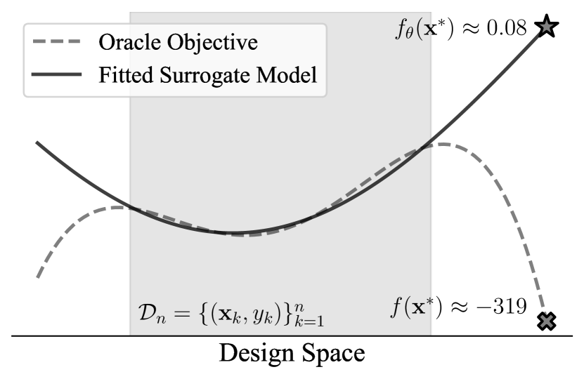
Figure 1: Objective overestimation in offline model-based optimization (MBO).    As described by Trabucco et al. (2021), naïve MBO optimizes against a learned surrogate function $f_{\theta}$ trained on a fixed dataset $\mathcal{D}_{n}=\{(\mathbf{x}_{i},y_{i})\}_{i=1}^{n}$ (shaded region) over a design space $\mathcal{X}$ without access to the true oracle $f$, often yielding candidate designs $\mathbf{x}^{*}$ that score poorly using the true oracle (i.e., cross). As an example, even though a surrogate model for molecule Penalized LogP (Ertl & Schuffenhauer, 2009) score prediction achieves a root mean squared error (RMSE) of approximately 0.24 on $\mathcal{D}_{n}$, its RMSE on design candidates generated through vanilla Bayesian optimization is approximately 114—over 400 times worse. Figure function values are for a single example generated molecule.

To overcome this limitation, recent work has investigated the utility of policy optimization in the offline setting, where we are unable to query the objective function during the optimization process and instead only have access to a set of prior observations of inputs and associated objective values (Trabucco et al., 2021; Mashkaria et al., 2023). While one may naïvely attempt to learn a surrogate black-box model from the prior observations that approximates the true oracle objective function, such models can suffer from overestimation errors, yielding falsely promising objective estimates for inputs not contained in the offline dataset. As a result, optimization against the surrogate objective, often referred to as model-based optimization (MBO), may yield low-scoring candidate designs according to the true oracle objective function—a key limitation of traditional policy optimization techniques in the offline setting (Fig. 1).

In this work, we propose a task-agnostic offline optimization policy that learns to optimize against a surrogate model while simultaneously remaining in-distribution when compared against a reference offline dataset. In this setting, the policy is rewarded for determining optima that are similar to reference datums, thereby minimizing overestimation error and allowing for more robust oracle function optimization in the offline setting. Inspired by the recent success in generative adversarial networks (Goodfellow et al., 2014), we accomplish this task by proposing a novel method that regularizes a surrogate objective model using a source critic actor, which we call source critic regularization (SCR).

Our key contributions are as follows: (1) we offer a novel approach of formulating the SCR problem as a constrained primal optimization problem, and show theoretically how this framework can be used to solve for the regularization strength in the dual space; and (2) we propose a computationally tractable method to dynamically adjust the strength of source critic regularization as a function of the optimization trajectory in the input space. Compared with prior methods, we show that our algorithm achieves the highest rank of 2.9 across a variety of tasks spanning multiple scientific domains, and most consistently proposes optimal design candidates better than prior real-world observations.

2 Related Work

Leveraging source critic model feedback for adversarial training of neural networks was first introduced by Goodfellow et al. (2014), where a generator and adversarial discriminator “play” a zero-sum minimax game to train a generative model. However, such a discriminator often suffers from mode collapse and training instability in practice. To overcome these limitations, Arjovsky et al. (2017) introduced the Wasserstein generative adversarial net (WGAN), which instead utilizes a source critic that learns to approximate the 1-Wasserstein distance between the generated and training distributions. However, WGANs and similar GAN networks in the literature primarily aim to generate samples that look in-distribution from a latent space prior, rather than optimize against an objective function. Nonetheless, we adapt their framework for Wasserstein distance estimation in our work.

In the field of optimization, Brookes et al. (2019) introduced a method for conditioning by adaptive sampling (CbAS) that learns a density model of the input space that is gradually adapted towards the optimal solution. However, such prior methods have focused primarily on low-dimensional optimization tasks in the online setting. More recently, Trabucco et al. (2021) introduced conservative objective models (COM) specifically proposed for offline optimization tasks; however, their method requires directly modifying the parameters of the surrogate function during optimization, which is not always feasible for any general task. Mashkaria et al. (2023) proposed Black-box Optimization Networks (BONET) to instead learn the dynamics of online optimization trajectories using a causally masked transformer model, and Krishnamoorthy et al. (2023) introduced Denoising Diffusion Optimization Models (DDOM) to learn the generative process via a diffusion model conditioned on the objective values. Furthermore, Yu et al. (2021) and Chen et al. (2022) describe Robust Model Adaptation (RoMA) and Bidirectional learning via infinite-width networks (BDI), respectively. RoMA regularizes the gradient of surrogate objective models by enforcing a local smoothness prior at the observed inputs, and BDI utilizes neural tangent kernels to learn bidirectional mappings between low- and high- scoring candidates. While these recent works propose promising algorithms for offline optimization tasks, they require expensive oracle query budgets that are often not achievable in practice—especially for potentially dangerous tasks such as patient care and other high-stakes applications.

3 Background

3.1 Offline Model-Based Optimization

In many real-world domains, we often seek to optimize an oracle objective function $f(\mathbf{x})$ over a space of candidates

$$\mathbf{x}^{*}=\text{argmax}_{\mathbf{x}\in\mathcal{X}}f(\mathbf{x})$$ (1)

Examples of such problems include optimizing certain desirable properties of molecules in molecular design (Guimaraes et al., 2017; Brown et al., 2019; Maus et al., 2022), and estimating the optimal therapeutic intervention for patient care in clinical medicine (Kim & Bastani, 2021; Berrevoets et al., 2022; Xu & Bastani, 2023). In practice, however, the true objective function $f$ may be costly to compute or even entirely unknown, making it difficult to query in optimizing (1). Instead, it is often more feasible to obtain access to a reference dataset of observations from nature $\mathcal{D}_{n}=\{(\mathbf{x}_{1},y_{1}),\ldots,(\mathbf{x}_{n},y_{n})\}$ where $y_{i}=f(\mathbf{x}_{i})$. Using $\mathcal{D}_{n}$, we can learn a regressor model $f_{\theta}$ parametrized by

$$\theta^{*}=\text{argmin}_{\theta}\enspace\mathbb{E}_{(\mathbf{x}_{i},y_{i})\sim\mathcal{D}_{n}}||f_{\theta}(\mathbf{x}_{i})-y_{i}||^{2}$$ (2)

as a surrogate for the true oracle objective $f(\mathbf{x})$. Rather than querying $f$ as in (1), we can instead solve the related optimization problem

$$\mathbf{x}^{*}=\text{argmax}_{\mathbf{x}\in\mathcal{X}}f_{\theta}(\mathbf{x})$$ (3)

with the hopes that optimizing against $f_{\theta}$ will also lead to desirable oracle values of $f$ as well. Solving (3) is often referred to as offline model-based optimization (MBO) for which a number of techniques have been developed, such as iterative first-order methods and Bayesian Optimization (BO) (Sun et al., 2020). More concretely, gradient ascent (Grad.) starts from an initial candidate $\mathbf{x}_{0}$ and iteratively samples new designs according to the recursive policy $\mathbf{x}_{t+1}=\mathbf{x}_{t}+\eta\nabla f_{\theta}(\mathbf{x}_{t})$, where $\eta$ is the rate of optimization.

Of note, it is difficult to guarantee the reliability of the model’s predictions for $\mathbf{x}\notin\mathcal{D}_{n}$ that are almost certainly encountered in the optimization trajectory. Thus, naïvely optimizing the surrogate objective $f_{\theta}$ can result in “optima” that are low-scoring according to the oracle objective $f$.

3.2 Bayesian Optimization Over Latent Spaces

Bayesian optimization (BO) is a sample-efficient framework for solving expensive black-box optimization problems (Mockus, 1982; Osborne et al., 2009; Snoek et al., 2012). At iteration $t$ of BO, one has access to observations $\mathcal{D}_{t}=\{(\mathbf{x}_{i},y_{i})\}_{i=1}^{t}$, where $y_{i}$ denotes the objective value of the input $x_{i}$. Typically, a Gaussian process (Rasmussen, 2003) is employed as the surrogate model to approximate the objective function using these inputs and values. An acquisition function is then used to strategically sample the next batch of candidates for evaluation and update the surrogate model with these new observations. To better adapt BO for high-dimensional problems, Eriksson et al. (2019) introduced Trust Region BO (TuRBO) to avoid over-exploration in complex search spaces.

In certain cases, the search space $\mathcal{X}$ may be discretized over a finite set of structured inputs, such as amino acid sequences or molecular strings. Instead of directly optimizing over $\mathcal{X}$, recent work leverages deep variational autoencoders (VAEs) to first map the input space into a continuous, often lower dimensional latent space $\mathcal{Z}$ and then optimizing over $\mathcal{Z}$ instead (Tripp et al., 2020; Deshwal & Doppa, 2021; Maus et al., 2022). More concretely, a VAE is composed of a two networks: (1) an encoder with parameters $\phi$ that learns an approximated posterior distribution $q_{\phi}(z|\mathbf{x})$ for $\mathbf{x}\in\mathcal{X},z\in\mathcal{Z}$; and (2) a decoder with parameters $\varphi$ that learns the conditional likelihood distribution $p_{\varphi}(\mathbf{x}|z)$ (Kingma & Welling, 2013). The encoder and decoder are co-trained to maximize the evidence lower bound (ELBO)

$$\text{ELBO}=\mathbb{E}_{z\sim q_{\phi}}\left[\log p_{\varphi}(\mathbf{x}|z)\right]-D_{\text{KL}}\left[q_{\phi}(z|\mathbf{x})\text{ }||\text{ }p(z)\right]$$ (4)

where $D_{\text{KL}}$ is the Kullback-Leibler (KL) divergence.

3.3 Wasserstein Metric Between Probability Distributions

The Wasserstein distance is a distance metric between any two probability distributions in $\mathbb{R}^{d}$, and is closely related to problems in optimal transport. We define the $p=1$ Wasserstein distance between a reference distribution $P$ and a generated distribution $Q$ using distance metric $d(\cdot,\cdot)$ as

$$W_{1}(P,Q)=\inf_{\gamma\in\Gamma(P,Q)}\mathbb{E}_{(z^{\prime},z)\sim\gamma}d(z^{\prime},z)$$ (5)

where $\Gamma$ is the set of all couplings of $P$ and $Q$. For empirical distributions where $p_{n}$ ($q_{n}$) is based on $n$ observations $\{z_{j}^{\prime}\}_{j=1}^{n}$ ($\{z_{i}\}_{i=1}^{n}$), (5) can be simplified to

$$W_{1}(p_{n},q_{n})=\inf_{\sigma}\frac{1}{n}\sum_{i=1}^{n}||z^{\prime}_{\sigma(i)}-z||$$ (6)

where the infimum is over all permutations $\sigma$ of $n$ elements. Leveraging the Kantorovich-Rubinstein duality theorem (Kantorovich & Rubinstein, 1958), (6) can be written as

$$W_{1}(p_{n},q_{n})=\frac{1}{K}\sup_{||c||_{L}\leq K}\mathbb{E}_{z^{\prime}\sim P}[c(z^{\prime})]-\mathbb{E}_{z\sim Q}[c(z)]$$ (7)

where $c(z)$ is a source critic and $||c||_{L}$ is the Lipschitz norm of $c(z)$. In the Wasserstein GAN (WGAN) model proposed by Arjovsky et al. (2017), a generative network and source critic are co-trained in a minimax game where the generator (critic) seeks to minimize (maximize) the Wasserstein distance between the training and generated distributions. Such an optimization schema enables the generator policy to learn the distribution of training samples from nature.

4 Framework for Generative Adversarial Bayesian Optimization

In this section, we describe our proposed framework, Generative Adversarial Bayesian Optimization (GABO), which uses a source critic model to dynamically regularize the BO objective for offline model-based optimization.

4.1 Constrained Optimization Formulation

In offline generative optimization, we aim to optimize against a surrogate objective function $f_{\theta}$. In order to ensure that we are achieving reliable estimates of the true, unknown oracle objective, we can add a regularization penalty to keep generated samples “similar” to those from the training dataset of $f_{\theta}$ according to an adversarial source critic trained to discriminate between generated and offline samples. That is, in contrast to the original optimization problem in (3), GABO instead constrains it according to

$$\begin{split}\text{minimize}_{z\in\mathcal{Z}}&\quad-f_{\theta}(z)\\ \text{subject to}&\quad\mathbb{E}_{z^{\prime}\in P}[c^{*}(z^{\prime})]-c^{*}(z)\leq 0\end{split}$$ (8)

over some configuration space $\mathcal{Z}\subseteq\mathbb{R}^{n}$, and where we define $c^{*}$ as a source critic model that maximizes $\mathbb{E}_{z^{\prime}\in P}[c^{*}(z^{\prime})]-\mathbb{E}_{z\in Q}[c^{*}(z)]$ over all $K$-Lipschitz functions. We can think of $\mathbb{E}_{z^{\prime}\in P}[c^{*}(z^{\prime})]-c^{*}(z)$ as the contribution of a particular generated datum $z$ to the overall $p=1$ Wasserstein distance between the generated candidate ($Q$) and reference ($P$) distributions of designs as in (7). In practice, we model $c^{*}$ as a fully connected neural net. Intuitively, the imposed constraint restricts the feasible search space to designs that score at least as in-distribution as the average sample in the offline dataset according to the source critic. Therefore, $c^{*}$ acts as an adversarial model to regularize the optimization policy. Of note, this additional constraint in (8) may be highly non-convex for general $c^{*}$, and so it is often impractical to directly apply (8) to any arbitrary BO policy.

4.2 Dual Formulation

To solve the implementation problem put forth above, we instead look to reformulate (8) in its dual space by first considering the Lagrangian $\mathcal{L}$ of the constrained problem:

$$\mathcal{L}\left(z;\lambda\right)=-f_{\theta}(z)+\lambda\left[\mathbb{E}_{z^{\prime}\in P}[c^{*}(z^{\prime})]-c^{*}(z)\right]$$ (9)

where $\lambda\geq 0$ is the Lagrange multiplier associated with the constraint in (8). We can also think of $\lambda$ as a hyperparameter that controls the relative strength of the source critic-penalty term: $\lambda=0$ equates to naïvely optimizing the surrogate objective, while $\lambda\gg 1$ asymptotically approaches a WGAN-like optimization policy. Minimizing $\mathcal{L}$ thus minimizes a relative sum of $-f_{\theta}$ and the Wasserstein distance contribution from any particular generated datum $z$ with relative weighting dictated by the hyperparameter $\lambda$. From duality, minimizing $\mathcal{L}$ over $z$ and simultaneously maximizing over $\lambda\in\mathbb{R}_{+}$ is equivalent to the original constrained problem in (8).

The challenge now is in determining this optimal value of $\lambda$: if $\lambda$ is too small, then the objective estimates may be unreliable; if $\lambda$ is too large, then the optimization trajectory may be unable to adequately explore the input space. Prior work by Trabucco et al. (2021) has previously explored the idea of formulating offline optimization problems as a similarly regularized Lagrangian (albeit with a separate regularization constraint), although their method treats $\lambda$ as a static hyperparameter that is tuned by hand. In contrast, our method GABO treats $\lambda$ as a dynamic parameter that can adapt to the optimization trajectory in real time.

4.3 Computing the Lagrange Multiplier $\lambda$

Continuing with our dual formulation of the constrained problem, the Lagrange dual function $g(\lambda)$ is defined as $g(\lambda)=\inf_{z\in\mathbb{R}^{n}}\mathcal{L}\left(z;\lambda\right)$. The $z=\hat{z}$ that minimizes the Lagrangian in the definition of $g$ is evidently a function of $\lambda$. To show this, we use the first-order condition that $\nabla_{z}\mathcal{L}=0$ at $z=\hat{z}$. Per (9), we have

$$\nabla_{z}\mathcal{L}(\hat{z};\lambda)=-\nabla_{z}f_{\theta}(\hat{z})-\lambda\nabla_{z}c^{*}(\hat{z})=0$$ (10)

In general, solving (10) for $\hat{z}$ is computationally intractable—especially in high-dimensional problems. Instead, we can approximate $\hat{z}$ by sampling over $\mathbb{R}^{n}$ to find a reasonable estimate according to

$$\begin{split}\hat{z}(\lambda)=\mathop{\mathrm{argmin}}_{z\in\mathbb{R}^{n}}\frac{1}{2}\left|\left|-\nabla_{z}f_{\theta}(z)-\lambda\nabla_{z}c^{*}(z)\right|\right|^{2}\end{split}$$ (11)

Our key insight is that although minimizing the loss term in (11) is not practically feasible when naïvely optimizing over the entirety of $\mathbb{R}^{n}$, we can instead choose to focus our attention on latent space coordinates with high associated probability according to the multivariate standard normal distribution $\mathcal{N}(0,I)$. This is because in optimization problems acting over the latent space of any variational autoencoder, the majority of the encoded information content is embedded according to $\mathcal{N}(0,I)$ due to the Kullback-Leibler (KL) divergence contribution to VAE training. Put simply, the encoder distribution $q_{\phi}(z|\mathbf{x})$ is trained so that $D_{\text{KL}}[q_{\phi}(z|\mathbf{x})||\mathcal{N}(0,I)]$ is optimized as a regularization term, where $p(z)=\mathcal{N}(0,I)$ here is the latent prior. We argue that it is thus sufficient enough to approximate $\hat{z}(\lambda)$ using a Monte Carlo sampling schema with random samples $\mathcal{Z}_{N}=(z_{1},z_{2},\ldots,z_{N})\sim\mathcal{N}(0,1)$:

$$\begin{split}\hat{z}(\lambda)\approx\mathop{\mathrm{argmin}}_{\mathcal{Z}_{N}\sim\mathcal{N}(0,1)}\frac{1}{2}\left|\left|-\nabla_{z}f_{\theta}(z)-\lambda\nabla_{z}c^{*}(z)\right|\right|^{2}\end{split}$$ (12)

Therefore, (8) can be rewritten as the Lagrange dual problem

$$\begin{split}\text{maximize}&\quad g(\lambda)=-f_{\theta}(\hat{z})\\ &\quad\quad+\lambda\left[\mathbb{E}_{z^{\prime}\in P}[c^{*}(z^{\prime})]-c^{*}(\hat{z})\right]\\ \text{subject to}&\quad\lambda\geq 0\end{split}$$ (13)

where $\hat{z}$ is as in (12). Defining the surrogate variable $\alpha$ such that $\lambda=\frac{\alpha}{1-\alpha}$, we can rewrite (13) as

$$\begin{split}\text{maximize}&\quad-(1-\alpha)f_{\theta}(\hat{z})\\ &\quad\quad+\alpha\left[\mathbb{E}_{z^{\prime}\in P}[c^{*}(z^{\prime})]-c^{*}(\hat{z})\right]\\ \text{subject to}&\quad 0\leq\alpha<1\end{split}$$ (14)

In practice, we discretize the search space for $\alpha$ to 200 evenly spaced points between 0 and 1 inclusive. From weak duality, finding the optimal solution to the dual problem in (13) provides a lower bound on the optimal solution to the primal problem in (8). We now have a deterministic method (Algorithm 1) for choosing the optimal $\alpha$ (and hence $\lambda$) adaptively during offline optimization, and refer to this method as Adaptive SCR herein.

Algorithm 1 Adaptive Source Critic Regularization (SCR)

  Input: differentiable surrogate objective $f_{\theta}:\mathbb{R}^{d}\rightarrow\mathbb{R}$, differentiable source critic $c:\mathbb{R}^{d}\rightarrow\mathbb{R}$, reference dataset $\mathcal{D}_{n}=\{z^{\prime}_{j}\}_{j=1}^{n}$, $\alpha$ step size $\Delta\alpha$, search budget $\mathcal{B}$, norm threshold $\tau$

  Sample candidates $\mathcal{Z}_{\mathcal{B}}\leftarrow\{z_{i}\}_{i=1}^{\mathcal{B}}\sim\mathcal{N}(0,I_{d})$

  Initialize $\alpha^{*}\leftarrow\text{None}$ and $g^{*}\leftarrow-\infty$

  for $\alpha$ in $\text{range}(\text{start}=0,\text{end}=1,\text{stepsize}=\Delta\alpha)$ do

     $z^{*}\leftarrow\text{argmin}_{z_{i}\in\mathcal{Z}_{\mathcal{B}}}||(1-\alpha)\nabla f_{\theta}(z_{i})+\alpha\nabla c(z_{i})||_{2}$

     if $||(1-\alpha)\nabla f_{\theta}(z^{*})+\alpha\nabla c(z^{*})||_{2}>\tau$ then

        continue        // Discard $\alpha$ if best norm exceeds $\tau$

     end if

     $g\leftarrow-(1-\alpha)f_{\theta}(z^{*})+\alpha\left[\mathbb{E}_{\mathcal{D}_{n}}[c(z^{\prime}_{j})]-c(z^{*})\right]$

     if $g>g^{*}$ then

        $\alpha^{*}\leftarrow\alpha$ and $g^{*}\leftarrow g$              // Implements (14)

     end if

  end for

  return $\alpha^{*}$

4.4 Overall Algorithm

Using Adaptive SCR, we now have a proposed method for dynamically computing $\alpha$ (and hence the Lagrange multiplier $\lambda$) of the constrained optimization problem in (8). We integrate our algorithm with any standard batched model-based Bayesian Optimization framework by optimizing the Lagrangian objective in (9) over the candidate design space as opposed to the original unconstrained objective $f_{\theta}$. We refer to this algorithm as Generative Adversarial Bayesian Optimization (GABO) (Algorithm 2). We implement GABO using a quasi-expected improvement (qEI) acquisition function, iterative sampling budget of $T=32$, sampling batch size of $b=64$, and an oracle query budget of $k=1$ evaluated on the top (i.e., 100th percentile) design candidate according to the surrogate function.

Unlike traditional BO algorithms, the optimization objective for GABO is time-varying and causally linked to past observations made during the optimization process via intermittent training of the source critic $c$. Prior works from Nyikosa et al. (2018) and Aglietti et al. (2022) have examined BO in the setting of dynamic objective functions, although have either entirely disregarded causal relationships between variables or only examined causality between inputs as opposed to inputs and the objective. While work in optimization against dynamic objectives is limited, we find that GABO nonetheless works well in practice.

Algorithm 2 Generative Adversarial BayesOpt (GABO)

  Input: surrogate objective $f_{\theta}:\mathbb{R}^{d}\rightarrow\mathbb{R}$, offline dataset $\mathcal{D}_{n}=\{z^{\prime}_{j}\}_{j=1}^{n}$, acquisition function $g$, iterative sampling budget $T$, sampling batch size $b$, number of generator steps per source critic training $n_{\text{generator}}$, oracle query budget $k$

  AdaptiveSCR Input: $\alpha$ step size $\Delta\alpha$, search budget $\mathcal{B}$, norm threshold $\tau$

  Define: Differentiable source critic $c:\mathbb{R}^{d}\rightarrow\mathbb{R}$

  Define: Lagrangian $\mathcal{L}(z;\alpha):\mathbb{R}^{d}\times\mathbb{R}\rightarrow\mathbb{R}$      // Eq. (9)

           $\mathcal{L}(z;\alpha)=-f_{\theta}(z)+\frac{\alpha}{1-\alpha}[\mathbb{E}_{z^{\prime}\sim\mathcal{D}_{n}}[c(z^{\prime})]-c(z)]$

  Sample candidates $\mathcal{Z}^{1}\leftarrow\{z^{1}_{i}\}_{i=1}^{b}\sim\text{SobolSequence}$

  // Train the source critic per Eq. (7) to optimality:

  $c\leftarrow\text{argmax}_{||c||_{L}\leq K}W_{1}(\mathcal{D}_{n},\mathcal{Z}^{1})$

     $=\text{argmax}_{||c||_{L}\leq K}\left[\mathbb{E}_{z^{\prime}\sim\mathcal{D}_{n}}[c(z^{\prime})]-\mathbb{E}_{z\sim\mathcal{Z}^{1}}[c(z)]\right]$

  $\alpha\leftarrow\textbf{AdaptiveSCR}(f_{\theta},c,\mathcal{D}_{n},\Delta\alpha,\mathcal{B},\tau)$       // Alg. (1)

  Evaluate candidates $\mathcal{Y}^{1}\leftarrow\{y^{1}_{i}\}_{i=1}^{b}=\{-\mathcal{L}(z^{1}_{i};\alpha)\}_{i=1}^{b}$

  Place Gaussian Process (GP) prior on $f_{\theta}$

  for $t$ in $2,3,\ldots,T$ do

     Update posterior on $f_{\theta}$ with $\mathcal{D}_{t-1}=\{(\mathcal{Z}^{m},\mathcal{Y}^{m})\}_{m=1}^{t-1}$

     Compute acquisition function $g$ using fitted posterior

     Sample candidates $\mathcal{Z}^{t}\leftarrow\{z_{i}^{t}\}_{i=1}^{b}$ according to $g$

     $\alpha\leftarrow\textbf{AdaptiveSCR}(f_{\theta},c,\mathcal{D}_{n},\Delta\alpha,\mathcal{B},\tau)$

     Evaluate samples $\mathcal{Y}^{t}\leftarrow\{y^{t}_{i}\}_{i=1}^{b}=\{-\mathcal{L}(z_{i}^{t};\alpha)\}_{i=1}^{b}$

     if $t\text{ mod }n_{\text{generator}}$ equals $0$ then

        // Train the source critic per Eq. (7) to optimality:

        $c\leftarrow\text{argmax}_{||c||_{L}\leq K}W_{1}(\mathcal{D}_{n},\mathcal{Z}^{t})$

           $=\text{argmax}_{||c||_{L}\leq K}\left[\mathbb{E}_{z^{\prime}\sim\mathcal{D}_{n}}[c(z^{\prime})]-\mathbb{E}_{z\sim\mathcal{Z}^{t}}[c(z)]\right]$

     end if

  end for

  return the top $k$ samples from the $T\times b$ observations

           $\mathcal{D}_{T}=\{\{(z^{m}_{i},y^{m}_{i})\}_{i=1}^{b}\}_{m=1}^{T}$ according to $y^{m}_{i}$

5 Experimental Evaluation

5.1 Datasets and Tasks

To evaluate our proposed GABO algorithm, we focus on a set of seven tasks spanning multiple domains with publicly available datasets in the field of offline model-based optimization. (1) The Branin function is a well-known synthetic benchmark function where the task is to maximize the two-dimensional objective $f_{br}(z_{1},z_{2})=a(z_{2}-bz_{1}^{2}+cz_{1}-r)^{2}+s(1-t)\cos z_{1}+s$ defined over the square domain $z_{1}\in[-5,10]$, $z_{2}\in[0,15]$ with $a=-1$, $b=5.1/4\pi^{2}$, $c=5/\pi$, $r=6$, $s=-10$, and $t=1/8\pi$. To construct the offline dataset, we sample 1000 points from the square domain and remove the top 20%-ile according to $f_{br}$ to make the task more challenging, following prior work from Mashkaria et al. (2023). (2) The LogP task is a well-studied optimization problem (Zhou et al., 2019; Chen et al., 2021; Flam-Shepherd et al., 2022) where we search over candidate molecules to maximize the penalized water-octanol partition coefficient (logP) score, which is an approximate measure of the molecule’s hydrophobicity (Ertl & Schuffenhauer, 2009) that also rewards structures that can be synthesized easily and feature minimal ring structures. We use the publicly available Guacamol benchmarking dataset from Brown et al. (2019) to implement this task.

Tasks (3) - (6) are derived from Design-Bench, a publicly available set of MBO benchmarking tasks (Trabucco et al., 2022): (3) TF-Bind-8 aims to maximize the transcription factor binding efficiency of an 8-base-pair DNA sequence (Barrera et al., 2016); (4) GFP the green fluorescence of a 237-amino-acid protein sequence (Brookes et al., 2019; Rao et al., 2019); (5) UTR the gene expression from a 50-base-pair 5’UTR DNA sequence (Sample et al., 2019; Angermueller et al., 2020); and (6) ChEMBL the mean corpuscular hemoglobin concentration (MCHC) biological response of a molecule using an offline dataset collected from the ChEMBL assay CHEMBL3885882 (Gaulton et al., 2012). While Trabucco et al. (2022) include additional tasks in Design-Bench, we chose to focus our attention on the four discrete tasks (TF-Bind-8, GFP, UTR, and ChEMBL) related to the life sciences for the purposes of this study.

Finally, (7) the Warfarin task uses the dataset of patients on warfarin medication from Consortium (2009) to estimate the optimal dose of warfarin given clinical and pharmacogenetic patient data. Of note, in contrast to tasks (1) - (7) and other traditional MBO tasks in prior literature (Trabucco et al., 2022), the Warfarin task is novel in that only a subset of the input design dimensions may be optimized over (i.e., warfarin dose) while the others remain fixed as conditioning variables (i.e., patient covariates). Such a task can therefore be thought of as conditional model-based optimization.

5.2 Policy Optimization and Evaluation

For all experiments, the surrogate objective model $f_{\theta}$ is a fully connected net with two hidden layers of size 2048 and LeakyReLU activations. $f_{\theta}$ takes as input a VAE-encoded latent space datum and returns the predicted objective function value as output. The VAE encoder and decoder backbone architectures vary by MBO task and are detailed in Table A1. Following Gómez-Bombarelli et al. (2018) and Maus et al. (2022), we co-train the VAE and surrogate objective models together using an Adam optimizer (Kingma & Ba, 2014) with a learning rate of $3\times 10^{-4}$ for all tasks.

The source critic agent $c$ in (8) is implemented as a fully connected net with two hidden layers with sizes equal to four (one) times the number of input dimensions for the first (second) layer. The model outputs a single scalar for any unbatched input. To constrain the Lipschitz norm of $c$ as in (7), we clamp the weights of the model between [-0.01, 0.01] after each optimization step as done by Arjovsky et al. (2017). The model is trained using gradient descent with a learning rate of 0.001 to maximize the empirical Wasserstein distance between the dataset and generated candidates in the VAE latent space.

During the Bayesian optimization process, we alternate between sampling a batch of $b=64$ new latent space datums according to the q-expected improvement (qEI) acquisition function (Bergstra et al., 2011) and training the source critic actor $c(z)$ to optimality, which is defined as no improvement to the Wasserstein distance $W_{1}$ in Algorithm 2 according to $c$ after a patience of $n=100$ consecutive weight updates. MBO methods were evaluated using a fixed surrogate query budget of 2048 (except for the Warfarin task, which used a budget of 1024 due to compute constraints), and the oracle scores of the top $k=1$ candidates according to the surrogate function (i.e., one-shot oracle evaluation) are reported across 5 random seeds. We find that training $c$ every $n_{\text{generator}}=4$ sampling steps is a good choice across all tasks assessed, similar to prior work (Arjovsky et al., 2017).

We evaluate our GABO method with Adaptive SCR against a number of pre-existing baseline algorithms, including vanilla Bayesian Optimization (BO-qEI) and gradient ascent (Grad.). We also evaluate the related Grad Min. and Grad. Mean methods, which train an ensemble of 5 surrogate models and use the minimum (or mean) surrogate score to calculate the gradient for each step of gradient ascent. We also compare our method against the more recently introduced algorithms TuRBO-qEI (Eriksson et al., 2019), COM (Trabucco et al., 2021), RoMA (Yu et al., 2021), BDI (Chen et al., 2022), DDOM (Krishnamoorthy et al., 2023), and BONET (Mashkaria et al., 2023). All methods were trained and evaluated on a single internal cluster with 8 NVIDIA RTX A6000 GPUs.

Table 1: One-Shot ($k=1$) Oracle Evaluation    Oracle scores across 5 random seeds reported as mean $\pm$ standard deviation. $\mathcal{D}$ (best) reports the top oracle value in the task dataset. Each of the MBO methods assessed below are ranked by their mean one-shot oracle score, and the average rank across all seven tasks is reported in the final table column. Bolded (Underlined) entries indicate the best (second best) entry in the column. ^∗Denotes the life sciences-related discrete MBO tasks from Design-Bench (Trabucco et al., 2022).

Method	Branin	LogP	TF-Bind-8∗	GFP∗	UTR∗	ChEMBL∗	Warfarin	Rank
$\mathcal{D}$ (best)	-13.0	11.3	0.439	3.53	7.12	0.605	-0.19 $\pm$ 1.96	—
Grad.	-20.3 $\pm$ 14.0	-4.94 $\pm$ 0.86	0.439 $\pm$ 0.00	3.60 $\pm$ 0.02	6.80 $\pm$ 0.38	-1.95 $\pm$ 0.00	0.91 $\pm$ 0.48	6.7
Grad. Mean	-9.4 $\pm$ 2.8	-4.71 $\pm$ 1.67	0.439 $\pm$ 0.00	3.62 $\pm$ 0.00	6.95 $\pm$ 0.40	-1.95 $\pm$ 0.00	0.95 $\pm$ 0.26	5.7
Grad. Min	-9.9 $\pm$ 3.1	-3.83 $\pm$ 0.87	0.439 $\pm$ 0.00	3.63 $\pm$ 0.02	7.04 $\pm$ 0.33	-1.95 $\pm$ 0.00	0.91 $\pm$ 0.56	5.3
BO-qEI	-2.5 $\pm$ 0.2	-65.2 $\pm$ 108	0.472 $\pm$ 0.11	1.43 $\pm$ 0.00	6.05 $\pm$ 1.33	0.579 $\pm$ 0.08	0.02 $\pm$ 0.10	6.7
TuRBO-qEI	-22.9 $\pm$ 1.1	-80.6 $\pm$ 122	0.534 $\pm$ 0.17	1.43 $\pm$ 0.00	6.33 $\pm$ 1.47	0.652 $\pm$ 0.00	0.02 $\pm$ 0.10	6.4
BONET	-26.1 $\pm$ 0.9	10.9 $\pm$ 0.15	0.447 $\pm$ 0.08	3.74 $\pm$ 0.00	8.92 $\pm$ 0.12	0.520 $\pm$ 0.12	—	4.2
DDOM	-8668 $\pm$ 1500	-3.46 $\pm$ 0.85	0.510 $\pm$ 0.15	1.43 $\pm$ 0.00	6.15 $\pm$ 1.47	0.564 $\pm$ 0.08	0.27 $\pm$ 0.82	6.9
COM	-3859 $\pm$ 80	34.0 $\pm$ 18.2	0.439 $\pm$ 0.00	3.62 $\pm$ 0.00	6.52 $\pm$ 0.68	0.648 $\pm$ 0.00	0.78 $\pm$ 0.33	5.1
RoMA	-275 $\pm$ 0.8	7.02 $\pm$ 1.87	0.415 $\pm$ 0.04	3.41 $\pm$ 0.28	6.44 $\pm$ 0.91	0.542 $\pm$ 0.04	-0.82 $\pm$ 0.24	7.9
BDI	-117 $\pm$ 0.0	10.4 $\pm$ 0.00	0.471 $\pm$ 0.00	3.67 $\pm$ 0.06	5.61 $\pm$ 0.00	0.492 $\pm$ 0.00	-24.8 $\pm$ 233	7.0
GABO (Ours)	-4.0 $\pm$ 1.5	19.6 $\pm$ 43.1	0.636 $\pm$ 0.07	3.74 $\pm$ 0.00	6.72 $\pm$ 0.49	0.612 $\pm$ 0.00	0.16 $\pm$ 0.29	2.9

Conditional MBO Tasks. To our knowledge, prior work in conditional model-based optimization is limited, and so previously reported algorithms are not equipped to solve such tasks out-of-the-box. Therefore, to assess existing methods on the conditional Warfarin task, we implement conditional proxies of all baselines employing a first-order optimization schema via partial gradient ascent to only update the warfarin dose dimension while leaving the patient attribute conditional dimensions unchanged. Conditional BO-qEI, TuRBO-qEI, and GABO are implemented by fitting separate Gaussian processes for each patient. Finally, in conditional DDOM, we exchange the algorithm’s diffusion model-based backbone with a conditional score-based diffusion model described by Batzolis et al. (2021) and Gu et al. (2023).

Of note, the BONET algorithm proposed by Mashkaria et al. (2023) requires multiple observations for any given patient to construct its synthetic optimization trajectories. However, the key challenge in conditional MBO is that each condition (i.e., patient) has no past observations (i.e., warfarin doses), and instead relies on learning from offline datasets constructed from different permutations of condition values for effective optimization. As a result, the BONET algorithm is unable to be evaluated on conditional MBO tasks.

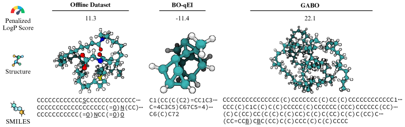
Figure 2: Penalized LogP Score Maximization Sample Candidate Designs    (Left) the molecule with the highest penalized LogP score of 11.3 in the offline dataset. Separately, we show the 100th percentile candidate molecules according to the surrogate objective generated from (Middle) vanilla BO-qEI and (Right) GABO with Adaptive SCR. Teal- (white-) colored atoms are carbon (hydrogen). Non-hydrocarbon atoms are underlined in the SMILES (Weininger, 1988) string representations of the molecules.

Table 2: Adaptive SCR Ablation Study    One-shot oracle evaluations averaged across 5 random seeds reported as mean $\pm$ standard deviation. $\mathcal{D}$ (best) reports the top oracle value in the task dataset. Average method rank across all seven tasks reported in the final column. ^∗Denotes the life sciences-related discrete MBO tasks offered by the Design-Bench benchmarking repository (Trabucco et al., 2022).

GABO $\alpha$ Value	Branin	LogP	TF-Bind-8∗	GFP∗	UTR∗	ChEMBL∗	Warfarin	Rank
$\mathcal{D}$ (best)	-13.0	11.3	0.439	3.53	7.12	0.605	-0.19 $\pm$ 1.96	—
0.0	-2.5 $\pm$ 0.2	-65.2 $\pm$ 108	0.472 $\pm$ 0.11	1.43 $\pm$ 0.00	6.05 $\pm$ 1.33	0.579 $\pm$ 0.08	0.02 $\pm$ 0.10	4.6
0.2	-2.2 $\pm$ 0.3	-28.2 $\pm$ 39.0	0.559 $\pm$ 0.12	1.42 $\pm$ 0.00	6.90 $\pm$ 0.64	0.612 $\pm$ 0.00	0.02 $\pm$ 0.10	3.0
0.5	-2.1 $\pm$ 0.4	-45.6 $\pm$ 41.5	0.601 $\pm$ 0.25	1.43 $\pm$ 0.00	6.66 $\pm$ 0.85	0.602 $\pm$ 0.02	0.02 $\pm$ 0.10	3.3
0.8	-2.3 $\pm$ 0.3	27.6 $\pm$ 37.1	0.696 $\pm$ 0.19	1.88 $\pm$ 0.93	5.33 $\pm$ 1.16	0.608 $\pm$ 0.01	0.02 $\pm$ 0.10	2.7
1.0	-67.2 $\pm$ 29.5	-4.29 $\pm$ 0.03	0.395 $\pm$ 0.09	3.73 $\pm$ 0.01	6.21 $\pm$ 1.64	0.597 $\pm$ 0.03	-0.60 $\pm$ 1.51	4.6
Adaptive SCR	-4.0 $\pm$ 1.5	19.6 $\pm$ 43.1	0.636 $\pm$ 0.07	3.74 $\pm$ 0.00	6.72 $\pm$ 0.49	0.612 $\pm$ 0.00	0.16 $\pm$ 0.29	2.0

5.3 Main Results

Scoring of one-shot optimization candidates is shown in Table 1. Across all seven assessed tasks spanning a wide range of scientific domains, GABO with Adaptive SCR achieved the highest average rank of 2.9 when compared to other existing methods. Furthermore, Adaptive SCR was able to propose top $k=1$ candidate designs that outperform the best design in the pre-existing offline dataset for 6 of the 7 tasks–greater than any of the other methods assessed. Our method performed best in two tasks (TF-Bind-8, GFP), and was one of the top 2 methods assessed for four tasks (Branin, LogP, TF-Bind-8, GFP).

Of note, the baseline method results reported in Table 1 are different than those reported in prior work (Trabucco et al., 2021; Mashkaria et al., 2023; Krishnamoorthy et al., 2023; Chen et al., 2022) due to differences in oracle evaluation budgets. All previously cited methods for offline MBO tasks report 100th percentile oracle scores using an oracle evaluation budget of either $k=128$ or $k=256$, which is often infeasible in many domains where offline MBO can be applied. (We nonetheless offer additional experimental results in this few-shot oracle evaluation setting discussed in Appendix B.) As an example, applying offline MBO methods to tasks such as patient medication dosing—as done in the Warfarin task—is a high-stakes exercise with little room for experimentation, as any individual patient can only be given one medication dose at a given point in time. To this end, our results demonstrate that GABO outperforms preexisting methods in the domain of one-shot oracle evaluation tasks, and is a viable method for proposing optimal design candidates in offline MBO.

5.4 Qualitative Evaluation: Penalized LogP Task

We evaluate GABO against naïve BO-qEI for the LogP task by inspecting the three-dimensional chemical structures of the top-scoring candidate molecules. As a general principle, molecules that are associated with high Penalized LogP scores are hydrophobic with minimal ring structures and therefore often feature long hydrocarbon backbones (Ertl & Schuffenhauer, 2009). In Figure 2, we see that BO-qEI using the unconstrained surrogate objective generates a candidate molecule of hydrogen and carbon atoms. However, the proposed candidate includes two rings in its structure, resulting in a suboptimal oracle Penalized LogP score.

We hypothesize that this may be due to a lack of ring-containing example molecules in the offline dataset, as only 6.7% (2.7%) of observed molecules contain at least one (two) carbon ring(s). As a result, the surrogate objective model estimator returns more inaccurate Penalized LogP estimates for input ring-containing structures (surrogate model root mean squared error (RMSE) = 25.5 for offline dataset molecules with at least 2 rings; RMSE = 16.5 for those with at least 1 ring; and RMSE = 4.6 for those with at least 0 rings), leading to sub-par BO-qEI optimization performance as the unconstrained algorithm finds “optimal” molecules that are out-of-distribution compared to the offline dataset. In contrast, our GABO method generates a candidate molecule with a long hydrocarbon backbone and no rings, resulting in a penalized logP score of 22.1—greater than the best observed value in the offline Guacamol dataset.

5.5 Ablation Experiments

Taking inspiration from (Trabucco et al., 2021), it is possible to utilize our GABO algorithm without dynamically computing the Lagrange multiplier $\lambda$. To better understand the utility of our Adaptive SCR algorithm within the offline GABO framework, we ablate Algorithm 1 by treating $\lambda$ instead as a tunable constant hyperparameter, and test our method using different values of $\lambda=\alpha/(1-\alpha)$ (Table 2). Setting $\alpha=0$ (i.e., $\lambda=0$) corresponds to naïve BO against the unconstrained surrogate model, while setting $\alpha=1$ (i.e., $\lambda\rightarrow\infty$) is equivalent to a WGAN-like sampling policy.

Evaluating constant values of $\alpha$ ranging from 0 to 1, we find that there is no consistently optimal constant value for all seven of the MBO tasks assessed in this study. In constrast, our method achieves an average rank of 2.0 and is one of the top two methods when compared to the ablations for six of the seven tasks. Additional ablation studies are included in Appendix B. Altogether, these results suggest our Adaptive SCR algorithm improves GABO performance in solving the general constrained optimization problem in (8).

Interestingly, the top designs found across different constant values of $\alpha$ can be very similar for certain tasks (i.e., Branin, ChEMBL, and Warfarin tasks in Table 2). This reflects the inherent challenge in developing task-agnostic methods for objective function regularization—if the magnitudes of the unconstrained objective and regularization function vastly differ, then constant values of $\alpha$ may over- or under- constrain the objective. In contrast, GABO combined with Adaptive SCR overcomes this limitation by dynamically adjusting $\alpha$ as an implicit function of prior observations.

6 Conclusion

We propose a novel framework that introduces a source critic adversary as a regularizing agent to solve the problem of off-distribution objective evaluation in offline model-based policy optimization. Our method, GABO with Adaptive SCR, dynamically adjusts the regularization strength according to the optimization trajectory, and consistently outperforms baseline methods to achieve an average rank of 2.9 in one-shot $k=1$ oracle evaluation when compared to the other MBO methods assessed, and most consistently proposes new candidate designs better than the offline dataset.

Limitations. One limitation of our Adaptive SCR algorithm (Algorithm 1) is that our approach requires preexisting knowledge of the prior distribution over the input space in order for the method to be computationally tractable. While we have focused our experimental evaluation on tasks amenable to imposed latent space priors, further work is needed to adapt GABO with Adaptive SCR to any arbitrary configuration space. We are also interested in extending our work to the online setting where a finite number of oracle queries may be allowed during optimization. Future work may also examine how our algorithm can be integrated with more sophisticated BO techniques, such as TuRBO (Eriksson et al., 2019) and BO with time- and trajectory- varying objectives (Nyikosa et al., 2018; Aglietti et al., 2022).

7 Impact Statement

Offline policy optimization methods, such as those discussed in this work, have the potential to benefit society. Such examples may include helping develop more effective drugs and individualizing patient therapies for precision medicine. However, as with any real-world algorithm, these methods can also be leveraged to generate potentially harmful design candidates—whether intentionally or inadvertently. Careful oversight by domain experts and researchers alike is required to ensure that the contributions proposed herein are used positively for social good.

Appendix A Additional Implementation Details

In this section, we offer additional insights into the design of the oracle functions and standard data preprocessing pipeline used in the seven model-based optimization (MBO) tasks assessed in this work.

Oracle Functions. All oracle functions for the seven tasks assessed are either exact functions or approximate oracles developed by domain experts. Specifically, the Branin and TF-Bind-8 tasks utilize exact oracles described in detail by Branin (1972) and Barrera et al. (2016), respectively. The oracle for the Penalized LogP task is an approximate oracle from Wildman & Crippen (1999) that uses an atom-based scheme to estimate the Penalized LogP score as a linear combination of the atomic features of an input molecule, and is the same oracle used by domain experts in the Guacamol benchmarking study (Brown et al., 2019). The GFP, UTR, and ChEMBL tasks feature approximate oracles from Snoek et al. (2012), Angermueller et al. (2020), and Trabucco et al. (2022), respectively, that were trained on a larger, hidden datasets inaccessible to us for the MBO tasks described herein. Finally, the Warfarin task uses a linear model (Consortium, 2009) to estimate a patient’s optimal warfarin dose given their pharmacogenetic attributes.

Data Preprocessing. (1) For the Branin task, we sample 1000 points from the square input domain $[-5,10]\times[0,15]$ and remove the top 20%-ile according to the oracle function to make the task more challenging, in line with prior work (Mashkaria et al., 2023). In this continuous task, we treat the Branin datums as their own latent space mappings, such that the VAE encoder and decoder for this task are both the identity function with zero trainable parameters. (2) Due to computational restrictions, we limit the offline dataset of the Penalized LogP task to the validation partition of the Guacamol dataset from Brown et al. (2019) consisting of 79,564 unique molecules and their corresponding penalized LogP values. The input molecules are represented as SMILES strings (Weininger, 1988), which is a molecule representation format that has been shown to frequently yield invalid molecules in prior work (Krenn et al., 2020). Therefore, we encode the molecules instead as SELFIES strings, an alternative molecule representation introduced by Krenn et al. (2020) with 100% robustness.

(3) - (5) The TF-Bind-8, GFP, and UTR tasks are assessed as-released by Design-Bench from Trabucco et al. (2022)—please refer to their work for task-specific descriptions. (6) In the ChEMBL task, we normalize all objective values $y$ in the offline dataset to $\hat{y}=(y-y_{\text{min}})/(y_{\text{max}}-y_{\text{min}})$ as done in prior work (Mashkaria et al., 2023), where $\hat{y}$ is the corresponding normalized objective value and $y_{\text{min}}$ ($y_{\text{max}}$) is the minimum (maximum) observed objective value in the full, unobserved dataset. Because the top 60%-ile from the unobserved dataset is used to construct the available offline dataset for the ChEMBL task, the maximum $\hat{y}$ value for the task is less than 1.0 (Table A1). Furthermore, we also translate the original SMILES string representations into SELFIES strings (Krenn et al., 2020), similar to the LogP task above.

(7) Finally, the Warfarin task uses the dataset of pharmacogenetic patient covariates published by Consortium (2009). We split the original dataset of 3,936 unique patient observations into training (validation) partitions with 3,736 (200) datums. The patient attributes in the Warfarin dataset consist of a combination of discrete and continuous values. All discrete attributes are one-hot encoded into binarized dimensions, and continuous values are normalized to zero mean and unit variance using the training dataset. Missing patient values were imputed following prior work (Truda & Marais, 2021). We define the cost $c(z|x)$ accrued by a patient with attributes $x\in\mathbb{R}^{32}$ as a function of the input dose $z\in\mathbb{R}$ is $c(z|x)=(z-d_{\text{oracle}}(x))^{2}$, where $d_{\text{oracle}}:\mathbb{R}^{32}\rightarrow\mathbb{R}$ is the domain-expert oracle warfarin dose estimator from Consortium (2009). The observed objective values $y$ associated with each of the training datums is calculated as $y=[c(\bar{z}|x)-c(z|x)]/c(\bar{z}|x)$, where $\bar{z}$ is the mean warfarin dose over the training dataset and $z$ is the true dose given to the patient. Using this constructed offline dataset, our task is then to assign optimal doses to the 200 validation patients to maximize $y$ with no prior warfarin dosing observations.

Table A1: MBO Datasets and Tasks    Implementation details for each of the seven MBO tasks assessed in our work. ^∗Denotes the life sciences-related discrete MBO tasks offered by the Design-Bench benchmarking repository (Trabucco et al., 2022).

Property	Branin	LogP	TF-Bind-8∗	GFP∗	UTR∗	ChEMBL∗	Warfarin
Dataset Size	800	79,564	32,898	5,000	140,000	441	200
Input Shape	2	108	8	237	50	32	1 (33)
Vocab Size	—	97	4	20	4	40	—
VAE Backbone	Identity	Transformer	ResNet	ResNet	ResNet	Transformer	Identity
VAE Latent Shape	2	256	16	32	32	128	33
Oracle	Exact	Linear	Exact	Transformer	ResNet	Random Forest	Linear
$\mathcal{D}$ (best)	-13.0	11.3	0.439	3.53	7.12	0.605	-0.19 $\pm$ 1.96

Appendix B Additional Experimental Results

Few-Shot Oracle Evaluation. In Section 5.3, we assess the GABO with Adaptive SCR and other offline MBO methods reported in prior work according to a one-shot (i.e., $k=1$ oracle query budget) evaluation schema (Table 1). More concretely, each method proposed a set of 2048 design candidates for each task—within each set, the candidates were ranked according to the method-specific surrogate function, and the top-performing (i.e., “one-shot”) candidate’s oracle score was reported. We chose to utilize this evaluation schema in Table 1 because in many high-stakes applications of offline optimization, it is often costly or even impossible to achieve more expensive compute budgets.

Nonetheless, in certain cases it may be possible to allow for multiple oracle queries. To this end, we also report few-shot 100th percentile results, which involves taking the top $k=64$ candidates (i.e., “few-shot”) according to the surrogate objective, evaluating these candidates according to the oracle, and reporting the maximum (i.e., 100th percentile) oracle score from the $k=64$ proposed candidates (Table B1). Across all seven offline optimization tasks, GABO with Adaptive SCR is the only method assessed that proposes a design candidate better than the reference designs from the offline dataset while achieving an average rank of 1.7. Separately, we also report one-shot 90th percentile evaluation metrics in Table B2. Corresponding results for ablating our Adaptive SCR algorithm are also shown in Table B3 and Table B4, respectively. Altogether, these results support the utility of our proposed algorithm for a variety of different offline MBO tasks.

Table B1: Few-Shot ($k=64$) Evaluation    The maximum oracle score across the top $k=64$ design candidates according to the surrogate objective is averaged across 5 random seeds and reported as mean $\pm$ standard deviation. $\mathcal{D}$ (best) reports the top oracle value in the task dataset. The average rank across all seven tasks is reported in the final table column. Bolded (Underlined) entries indicate the best (second best) entry in the column. ^∗Denotes the life sciences-related discrete MBO tasks from Design-Bench (Trabucco et al., 2022).

Method	Branin	LogP	TF-Bind-8∗	GFP∗	UTR∗	ChEMBL∗	Warfarin	Rank
$\mathcal{D}$ (best)	-13.0	11.3	0.439	3.53	7.12	0.605	-0.19 $\pm$ 1.96	—
Grad.	-3.7 $\pm$ 0.8	-4.49 $\pm$ 1.38	0.439 $\pm$ 0.00	3.72 $\pm$ 0.00	7.43 $\pm$ 0.26	-1.953 $\pm$ 0.00	0.91 $\pm$ 0.48	7.4
Grad. Mean	-4.3 $\pm$ 0.6	-3.94 $\pm$ 1.44	0.439 $\pm$ 0.00	3.72 $\pm$ 0.00	7.44 $\pm$ 0.14	-1.953 $\pm$ 0.00	0.95 $\pm$ 0.26	7.4
Grad. Min	-4.1 $\pm$ 0.6	-3.74 $\pm$ 0.85	0.439 $\pm$ 0.00	3.72 $\pm$ 0.00	7.42 $\pm$ 0.20	-1.953 $\pm$ 0.00	0.91 $\pm$ 0.56	7.4
BO-qEI	-0.5 $\pm$ 0.1	130 $\pm$ 19.6	0.941 $\pm$ 0.03	1.43 $\pm$ 0.00	8.20 $\pm$ 0.07	0.662 $\pm$ 0.01	1.00 $\pm$ 0.00	3.4
TuRBO-qEI	-2.2 $\pm$ 3.2	39.2 $\pm$ 55.7	0.873 $\pm$ 0.05	1.43 $\pm$ 0.00	7.97 $\pm$ 0.32	0.672 $\pm$ 0.01	0.94 $\pm$ 0.08	4.6
BONET	-26.0 $\pm$ 0.9	11.6 $\pm$ 0.26	0.496 $\pm$ 0.07	3.74 $\pm$ 0.00	9.18 $\pm$ 0.05	0.650 $\pm$ 0.01	—	4.7
DDOM	-0.5 $\pm$ 0.2	-2.53 $\pm$ 0.70	0.579 $\pm$ 0.15	1.44 $\pm$ 0.00	8.14 $\pm$ 0.12	0.585 $\pm$ 0.04	1.00 $\pm$ 0.00	5.7
COM	-3255 $\pm$ 112	36.8 $\pm$ 19.6	0.439 $\pm$ 0.00	3.62 $\pm$ 0.00	6.82 $\pm$ 0.77	0.648 $\pm$ 0.00	0.79 $\pm$ 0.32	8.3
RoMA	-8.9 $\pm$ 0.2	9.60 $\pm$ 1.01	0.631 $\pm$ 0.14	3.73 $\pm$ 0.01	8.16 $\pm$ 0.15	0.669 $\pm$ 0.04	0.55 $\pm$ 0.05	5.3
BDI	-86.6 $\pm$ 0.0	10.4 $\pm$ 0.00	0.471 $\pm$ 0.00	3.67 $\pm$ 0.06	5.61 $\pm$ 0.00	0.492 $\pm$ 0.00	-24.8 $\pm$ 233	8.4
GABO (Ours)	-0.5 $\pm$ 0.1	96.1 $\pm$ 43.9	0.948 $\pm$ 0.02	3.74 $\pm$ 0.00	8.30 $\pm$ 0.14	0.665 $\pm$ 0.01	1.00 $\pm$ 0.00	1.7

Table B2: One-Shot ($k=1$) 90th Percentile Evaluation    The oracle score of the 90th percentile design candidate according to the surrogate across 5 random seeds is reported as mean $\pm$ standard deviation. $\mathcal{D}$ (best) reports the top oracle value in the task dataset. The average rank across all seven tasks is reported in the final table column. Bolded (Underlined) entries indicate the best (second best) entry in the column. ^∗Denotes the life sciences-related discrete MBO tasks from Design-Bench (Trabucco et al., 2022).

Method	Branin	LogP	TF-Bind-8∗	GFP∗	UTR∗	ChEMBL∗	Warfarin	Rank
$\mathcal{D}$ (best)	-13.0	11.3	0.439	3.53	7.12	0.605	-0.19 $\pm$ 1.96	—
Grad.	-43.5 $\pm$ 2.2	-4.93 $\pm$ 0.86	0.439 $\pm$ 0.00	3.64 $\pm$ 0.05	6.91 $\pm$ 0.42	-1.95 $\pm$ 0.00	0.91 $\pm$ 0.48	5.9
Grad. Mean	-46.4 $\pm$ 2.1	-4.08 $\pm$ 1.28	0.439 $\pm$ 0.00	3.67 $\pm$ 0.03	6.68 $\pm$ 0.64	-1.95 $\pm$ 0.00	0.95 $\pm$ 0.26	5.6
Grad. Min	-11.7 $\pm$ 0.3	-4.31 $\pm$ 1.42	0.439 $\pm$ 0.00	3.67 $\pm$ 0.06	6.62 $\pm$ 0.77	-1.95 $\pm$ 0.00	0.91 $\pm$ 0.56	5.9
BO-qEI	-7.3 $\pm$ 5.0	-78.1 $\pm$ 152	0.449 $\pm$ 0.07	1.42 $\pm$ 0.01	5.78 $\pm$ 1.83	0.604 $\pm$ 0.08	0.05 $\pm$ 0.11	7.0
TuRBO-qEI	-14.3 $\pm$ 9.8	-48.7 $\pm$ 64.7	0.557 $\pm$ 0.09	1.42 $\pm$ 0.00	6.72 $\pm$ 1.44	0.650 $\pm$ 0.00	0.49 $\pm$ 0.10	5.4
BONET	-26.8 $\pm$ 1.1	10.9 $\pm$ 0.47	0.444 $\pm$ 0.10	3.74 $\pm$ 0.00	9.12 $\pm$ 0.05	0.537 $\pm$ 0.07	—	3.5
DDOM	-4507 $\pm$ 7650	-7.49 $\pm$ 1.49	0.437 $\pm$ 0.16	1.43 $\pm$ 0.00	6.07 $\pm$ 0.59	0.597 $\pm$ 0.03	-5.26 $\pm$ 8.82	8.7
COM	-3126 $\pm$ 1023	-27.6 $\pm$ 9.3	0.439 $\pm$ 0.00	3.62 $\pm$ 0.00	6.73 $\pm$ 0.88	0.638 $\pm$ 0.01	0.78 $\pm$ 0.33	6.3
RoMA	-11.7 $\pm$ 0.3	5.56 $\pm$ 0.36	0.405 $\pm$ 0.07	3.61 $\pm$ 0.07	6.76 $\pm$ 1.60	0.556 $\pm$ 0.08	-2.36 $\pm$ 0.96	6.0
BDI	-108.7 $\pm$ 0.0	10.4 $\pm$ 0.00	0.471 $\pm$ 0.00	3.67 $\pm$ 0.06	5.61 $\pm$ 0.00	0.492 $\pm$ 0.00	-24.8 $\pm$ 233	6.4
GABO (Ours)	-5.3 $\pm$ 4.2	-5.54 $\pm$ 66.2	0.554 $\pm$ 0.08	2.58 $\pm$ 1.16	7.01 $\pm$ 0.82	0.629 $\pm$ 0.03	0.36 $\pm$ 0.48	4.1

Table B3: Adaptive SCR Ablation Study—Few-Shot ($k=64$) Evaluation    The maximum oracle score across the top $k=64$ design candidates according to the surrogate objective is averaged across 5 random seeds and reported as mean $\pm$ standard deviation. $\mathcal{D}$ (best) reports the top oracle value in the task dataset. Average method rank across all seven tasks reported in the final column. ^∗Denotes the life sciences-related discrete MBO tasks offered by the Design-Bench benchmarking repository (Trabucco et al., 2022).

GABO $\alpha$ Value	Branin	LogP	TF-Bind-8∗	GFP∗	UTR∗	ChEMBL∗	Warfarin	Rank
$\mathcal{D}$ (best)	-13.0	11.3	0.439	3.53	7.12	0.605	-0.19 $\pm$ 1.96	—
0.0	-0.48 $\pm$ 0.1	130 $\pm$ 19.6	0.941 $\pm$ 0.03	1.43 $\pm$ 0.00	8.20 $\pm$ 0.07	0.662 $\pm$ 0.01	1.00 $\pm$ 0.00	3.3
0.2	-0.49 $\pm$ 0.1	82.2 $\pm$ 43.2	0.893 $\pm$ 0.04	1.89 $\pm$ 0.92	8.19 $\pm$ 0.10	0.661 $\pm$ 0.01	1.00 $\pm$ 0.00	4.4
0.5	-0.46 $\pm$ 0.1	96.8 $\pm$ 25.1	0.909 $\pm$ 0.05	2.82 $\pm$ 1.12	8.17 $\pm$ 0.11	0.657 $\pm$ 0.01	1.00 $\pm$ 0.00	4.3
0.8	-0.43 $\pm$ 0.0	69.7 $\pm$ 10.2	0.923 $\pm$ 0.01	3.74 $\pm$ 0.00	8.25 $\pm$ 0.20	0.658 $\pm$ 0.00	1.00 $\pm$ 0.00	3.0
1.0	-1.2 $\pm$ 0.3	109 $\pm$ 14.8	0.861 $\pm$ 0.05	3.74 $\pm$ 0.00	8.24 $\pm$ 0.15	0.671 $\pm$ 0.02	0.47 $\pm$ 5.20	3.9
Adaptive SCR	-0.52 $\pm$ 0.1	96.1 $\pm$ 43.9	0.948 $\pm$ 0.02	3.74 $\pm$ 0.00	8.30 $\pm$ 0.14	0.665 $\pm$ 0.01	1.00 $\pm$ 0.00	2.1

Table B4: Adaptive SCR Ablation Study—One-Shot ($k=1$) 90th Percentile Evaluation    The oracle score of the 90th percentile design candidate according to the surrogate across 5 random seeds reported as mean $\pm$ standard deviation. $\mathcal{D}$ (best) reports the top oracle value in the task dataset. Average method rank across all seven tasks reported in the final column. ^∗Denotes the life sciences-related discrete MBO tasks from the Design-Bench benchmark (Trabucco et al., 2022).

GABO $\alpha$ Value	Branin	LogP	TF-Bind-8∗	GFP∗	UTR∗	ChEMBL∗	Warfarin	Rank
$\mathcal{D}$ (best)	-13.0	11.3	0.439	3.53	7.12	0.605	-0.19 $\pm$ 1.96	—
0.0	-7.3 $\pm$ 5.0	-78.1 $\pm$ 152	0.449 $\pm$ 0.07	1.42 $\pm$ 0.01	5.78 $\pm$ 1.83	0.604 $\pm$ 0.08	0.05 $\pm$ 0.11	3.7
0.2	-11.6 $\pm$ 5.0	-115 $\pm$ 215	0.505 $\pm$ 0.09	1.42 $\pm$ 0.00	6.08 $\pm$ 1.24	0.596 $\pm$ 0.08	0.04 $\pm$ 0.11	3.7
0.5	-9.6 $\pm$ 4.7	-128 $\pm$ 206	0.484 $\pm$ 0.12	1.42 $\pm$ 0.00	7.33 $\pm$ 0.96	0.536 $\pm$ 0.16	0.14 $\pm$ 0.16	4.0
0.8	-8.2 $\pm$ 5.0	4.83 $\pm$ 37.8	0.495 $\pm$ 0.16	1.42 $\pm$ 0.00	5.54 $\pm$ 1.93	0.559 $\pm$ 0.15	0.00 $\pm$ 0.09	3.6
1.0	-42.4 $\pm$ 46.3	-6.42 $\pm$ 1.90	0.301 $\pm$ 0.11	2.35 $\pm$ 1.14	4.94 $\pm$ 1.41	0.586 $\pm$ 0.06	-8.39 $\pm$ 11.0	4.7
Adaptive SCR	-5.3 $\pm$ 4.2	-5.54 $\pm$ 66.2	0.554 $\pm$ 0.08	2.58 $\pm$ 1.16	7.01 $\pm$ 0.82	0.629 $\pm$ 0.03	0.36 $\pm$ 0.48	1.3

Oracle Query Budget Ablation. To better characterize the performance of GABO as a function of the oracle query budget, we vary the number of allowed $k$-shot oracle calls in the Penalized LogP task (Figure B1). While first-order methods based on evaluating the first derivative of the surrogate objective are able to reach local optima rapidly, the proposed designs from such approaches are suboptimal compared to those from GABO with Adaptive SCR as the oracle query budget size increases. Comparing the curves for GABO and vanilla BO-qEI, we see that GABO with Adaptive SCR is able to propose consistently superior design candidates in the small query budget regime often encountered in real-world settings. This is due to the fact that GABO regularizes the surrogate function estimates such that the proposed candidates are both high-scoring according to the surrogate objective and relatively in-distribution. Our results demonstrate that especially for real-world tasks like molecule design with complex objective function landscapes, methods such as GABO with Adaptive SCR are able to explore diverse, high-performing design candidates effectively even in the setting of small oracle query budgets.

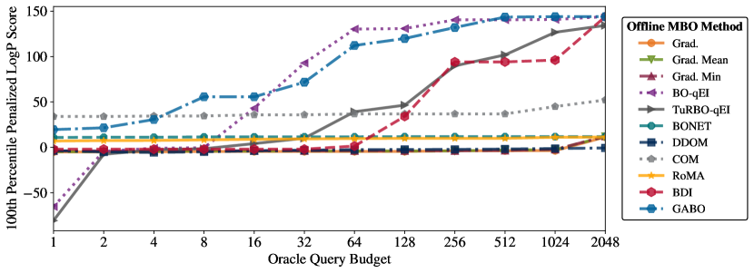
Figure B1: 100th Percentile Oracle Scores versus $k$-Shot Oracle Budget Size    We plot the 100th percentile oracle Penalized LogP score averaged across 5 random seeds as a function of the number of allowed oracle calls $k$. Note the logarithmic $x$-axis scaling.

Distance Covariance Analysis of GABO versus BO-qEI. A key feature of GABO with Adapative SCR is generated designs score similarly according to the hidden oracle function and the regularized Lagrangian objective as in (9) in order to solve the problem of surrogate objective overestimation encountered in traditional offline optimization settings (Fig 1). To assess this quantitatively, we computed the distance covariance $\text{dCov}_{n}[\{\mathcal{L}(\mathbf{x}_{k};\lambda^{*})\}_{k=1}^{n},\{f(\mathbf{x}_{k})\}_{k=1}^{n}]$ between the oracle scores $f(\mathbf{x}_{k})$ and the constrained Lagrangian scores $\mathcal{L}(\mathbf{x}_{k};\lambda^{*})$ with $\lambda=\lambda^{*}(t)$ computed using our Adaptive SCR algorithm. The empirical distance covariance metric is computed over the $n=2048$ design candidates generated using our GABO algorithm. Briefly, the distance covariance is a nonnegative measure of dependence between two vectors which may be related nonlinearly; a greater distance covariance implies a greater degree of association between observations (Székely et al., 2007). We focus our subsequent discussion on the Penalized LogP task.

Across five random seeds, GABO with Adaptive SCR achieves a distance covariance score of 0.535 $\pm$ 0.067 (mean $\pm$ standard deviation). In contrast, naïve BO-qEI (i.e., $\lambda=0$) only achieves a distance covariance score of 0.392 $\pm$ 0.040. Using $p<0.05$ as a cutoff for statistical significance, the distance covariance scores are significantly different between these two methods ($p\approx 0.006$, unpaired two-tailed $t$-test). These results help support our conclusion that GABO with Adaptive SCR is able to provide better estimates of design candidate performance according to the hidden oracle function when compared to the corresponding unconstrained BO policy.

References

- Aglietti et al. (2022) Aglietti, V., Dhir, N., González, J., and Damoulas, T. Dynamic causal Bayesian optimization. In Proc NeurIPS, 2022. doi: 10.48550/arXiv.2110.13891.
- Angermueller et al. (2020) Angermueller, C., Belanger, D., Gane, A., Mariet, Z., Dohan, D., Murphy, K., Colwell, L., and Sculley, D. Population-based black-box optimization for biological sequence design. In Proceedings of the 37th International Conference on Machine Learning, volume 119 of ICML’20, pp. 324–34. PMLR, 2020.
- Arjovsky et al. (2017) Arjovsky, M., Chintala, S., and Bottou, L. Wasserstein generative adversarial networks. In Proceedings of the 34th International Conference on Machine Learning, volume 70 of ICML’17, pp. 214–23. PMLR, 2017.
- Barrera et al. (2016) Barrera, L. A., Vedenko, A., Kurland, J. V., Rogers, J. M., Gisselbrecht, S. S., Rossin, E. J., Woodard, J., Mariani, L., Kock, K. H., Inukai, S., Siggers, T., Shokri, L., Gordân, R., Sahni, N., Cotsapas, C., Hao, T., Yi, S., Kellis, M., Daly, M. J., Vidal, M., Hill, D. E., and Bulyk, M. L. Survey of variation in human transcription factors reveals prevalent DNA binding changes. Science, 351(6280):1450–4, 2016. doi: 10.1126/science.aad2257.
- Bastani et al. (2021) Bastani, H., Drakopoulos, K., Gupta, V., Vlachogiannis, I., Hadjichristodoulou, C., Lagiou, P., Magiorkinis, G., Paraskevis, D., and Tsiodras, S. Efficient and targeted COVID-19 border testing via reinforcement learning. Nature, 599:108–13, 2021. doi: 10.1038/s41586-021-04014-z.
- Batzolis et al. (2021) Batzolis, G., Stanczuk, J., Schönlieb, C., and Etmann, C. Conditional image generation with score-based diffusion models. arXiv Preprint, 2021. doi: 10.48550/arXiv.2111.13606.
- Bergstra et al. (2011) Bergstra, J., Bardenet, R., Bengio, Y., and Kégl, B. Algorithms for hyper-parameter optimization. In Proc NeurIPS, volume 24, pp. 2546–54, 2011. doi: 10.5555/2986459.2986743.
- Berrevoets et al. (2022) Berrevoets, J., Verboven, S., and Verbeke, W. Treatment effect optimisation in dynamic environments. Journal of Causal Inference, 10(1):106–22, 2022. doi: 10.1515/jci-2020-0009.
- Branin (1972) Branin, F. H. Widely convergent method for finding multiple solutions of simultaneous nonlinear equations. IBM Journal of Research and Development, 16(5):504–22, 1972. doi: 10.1147/rd.165.0504.
- Brookes et al. (2019) Brookes, D., Park, H., and Listgarten, J. Conditioning by adaptive sampling for robust design. In Proceedings of the 36th International Conference on Machine Learning, volume 97 of ICML’19, pp. 773–82. PMLR, 2019.
- Brown et al. (2019) Brown, N., Fiscato, M., Segler, M. H. S., and Vaucher, A. C. GuacaMol: Benchmarking models for de novo molecular design. Journal of Chemical Information and Modeling, 59:1096–108, 2019. doi: 10.1021/acs.jcim.8b00839.
- Chen et al. (2022) Chen, C., Zhang, Y., Fu, J., Liu, X., and Coates, M. Bidirectional learning for offline infinite-width model-based optimization. In Proc NeurIPS, 2022. doi: 10.48550/arXiv.2209.07507.
- Chen et al. (2021) Chen, Z., Min, M. R., Parthasarathy, S., and Ning, X. A deep generative model for molecule optimization via one fragment modification. Nat Mach Intell, 3:1040–9, 2021. doi: 10.1038/s42256-021-00410-2.
- Consortium (2009) Consortium, T. I. W. P. Estimation of the warfarin dose with clinical and pharmacogenetic data. New England Journal of Medicine, 360(8):753–64, 2009. doi: 10.1056/NEJMoa0809329.
- Deshwal & Doppa (2021) Deshwal, A. and Doppa, J. Combining latent space and structured kernels for Bayesian optimization over combinatorial spaces. In Proc NeurIPS, volume 34, pp. 8185–200, 2021.
- Eriksson et al. (2019) Eriksson, D., Pearce, M., Gardner, J., Turner, R. D., and Poloczek, M. Scalable global optimization via local Bayesian optimization. In Proc NeurIPS, pp. 5496–507, 2019. doi: 10.48550/arXiv.1910.01739.
- Ertl & Schuffenhauer (2009) Ertl, P. and Schuffenhauer, A. Estimation of synthetic accessibility score of drug-like molecules based on molecular complexity and fragment contributions. J Cheminform, 1(8), 2009. doi: 10.1186/1758-2946-1-8.
- Flam-Shepherd et al. (2022) Flam-Shepherd, D., Zhu, K., and Aspuru-Guzik, A. Language models can learn complex molecule distributions. Nature Communications, 13(3293), 2022. doi: 10.1038/s41467-022-30839-x.
- Gaulton et al. (2012) Gaulton, A., Bellis, L. J., Bento, A. P., Chambers, J., Davies, M., Hersey, A., Light, Y., McGlinchey, S., Michalovich, D., Al-Lazikani, B., and Overington, J. P. ChEMBL: A large-scale bioactivity database for drug discovery. Nucleic Acids Res, 40:D1100–7, 2012. doi: 10.1093/nar/gkr777.
- Gómez-Bombarelli et al. (2018) Gómez-Bombarelli, R., Wei, J. N., Duvenaud, D., Hernández-Lobato, J. M., Sánchez-Lengeling, B., Sheberla, D., Aguilera-Iparraguirre, J., Hirzel, T. D., Adams, R. P., and Aspuru-Guzik, A. Automatic chemical design using a data-driven continuous representation of molecules. ACS Central Science, 4:268–76, 2018. doi: 10.1021/acscentsci.7b00572.
- Goodfellow et al. (2014) Goodfellow, I., Pouget-Abadie, J., Mirza, M., Xu, B., Warde-Farley, D., Ozair, S., Courville, A., and Bengio, Y. Generative adversarial nets. In Proc NeurIPS, pp. 2672–80, 2014. doi: 10.48550/arXiv.1406.2661.
- Gu et al. (2023) Gu, X., Yang, L., Sun, J., and Xu, Z. Optimal transport-guided conditional score-based diffusion models. In Proc NeurIPS, 2023. doi: 10.48550/arXiv.2311.01226.
- Guimaraes et al. (2017) Guimaraes, G. L., Sanchez-Lengeling, B., Outeiral, C., Farias, P. L. C., and Aspuru-Guzik, A. Objective-reinforced generative adversarial networks (ORGAN) for sequence generation models. arXiv Preprint, 2017. doi: 10.48550/arXiv.1705.10843.
- Kantorovich & Rubinstein (1958) Kantorovich, L. and Rubinstein, G. S. On a space of totally additive functions. Vestnik Leningrad. Univ, 13:52–9, 1958.
- Kim & Bastani (2021) Kim, C. and Bastani, O. Learning interpretable models with causal guarantees. arXiv Preprint, 2021. doi: 10.48550/arXiv.1901.08576.
- Kingma & Ba (2014) Kingma, D. P. and Ba, J. Adam: A method for stochastic optimization. In Proceedings of the 3rd International Conference on Learning Representations, 2014. doi: 10.48550/arXiv.1412.6980.
- Kingma & Welling (2013) Kingma, D. P. and Welling, M. Auto-encoding variational bayes. arXiv Preprint, 2013. doi: 10.48550/arXiv.1312.6114.
- Krenn et al. (2020) Krenn, M., Häse, F., Nigam, A., Friederick, P., and Aspuru-Guzik, A. Self-referencing embedded strings (selfies): A 100% robust molecular string representation. Machine Learning: Science and Technology, 1(4):045024, 2020. doi: 10.1088/2632-2153/aba947.
- Krishnamoorthy et al. (2023) Krishnamoorthy, S., Mashkaria, S., and Grover, A. Diffusion models for black-box optimization. In Proceedings of the 40th International Conference on Machine Learning, volume 202 of ICML’23, pp. 17842–57. JMLR, 2023.
- Mashkaria et al. (2023) Mashkaria, S., Krishnamoorthy, S., and Grover, A. Generative pretraining for black-box optimization. In Proceedings of the 40th International Conference on Machine Learning, volume 202 of ICML’23, pp. 24173–97. JMLR, 2023.
- Maus et al. (2022) Maus, N. T., Jones, H. T., Moore, J. S., Kusner, M. J., Bradshaw, J., and Gardner, J. R. Local latent space Bayesian optimization over structured inputs. In Proc NeurIPS, 2022. doi: 10.48550/arXiv.2201.11872.
- Mockus (1982) Mockus, J. The Bayesian approach to global optimization. In System Modeling and Optimization, pp. 473–481. Springer, 1982.
- Nyikosa et al. (2018) Nyikosa, F. M., Osborne, M. A., and Roberts, S. T. Bayesian optimization for dynamic problems. arXiv Preprint, 2018. doi: 10.48550/arXiv.1803.03432.
- Osborne et al. (2009) Osborne, M. A., Garnett, R., and Roberts, S. J. Gaussian processes for global optimization. In 3rd International Conference on Learning and Intelligent Optimization (LION3), pp. 1–15, 2009.
- Ramchandani et al. (2021) Ramchandani, P., Bastani, H., and Wyatt, E. Unmasking human trafficking risk in commercial sex supply chains with machine learning. Social Science Research Network, 2021. doi: 10.2139/ssrn.3866259.
- Rao et al. (2019) Rao, R., Bhattacharya, N., Thomas, N., Duan, Y., Chen, X., Canny, J., Abbeel, P., and Song, Y. S. Evaluating protein transfer learning with TAPE. In Proceedings of the 33rd International Conference on Neural Information Processing Systems, 2019. doi: 10.48550/arXiv.1906.08230.
- Rasmussen (2003) Rasmussen, C. E. Gaussian processes in machine learning. In Summer School on Machine Learning, pp. 63–71. Springer, 2003.
- Sample et al. (2019) Sample, P. J., Wang, B., Reid, D. W., Presnyak, V., McFadyen, I. J., Morris, D. R., and Seelig, G. Human 5’UTR design and variant effect prediction from a massively parallel translation study. Nature Biotechnology, 37:803–9, 2019. doi: 10.1038/s41587-019-0164-5.
- Snoek et al. (2012) Snoek, J., Larochelle, H., and Adams, R. P. Practical Bayesian optimization of machine learning algorithms. In Proc NeurIPS, volume 25, pp. 2951–9, 2012. doi: 10.48550/arXiv.1206.2944.
- Sun et al. (2020) Sun, S., Cao, Z., Zhu, H., and Zhao, J. A survey of optimization methods from a machine learning perspective. IEEE Transactions on Cybernetics, 50(8):3668–81, 2020. doi: 10.1109/TCYB.2019.2950779.
- Székely et al. (2007) Székely, G. J., Rizzo, M. L., and Bakirov, N. K. Measuring and testing dependence by correlation of distances. Annals of Statistics, 35(6):2769–94, 2007. doi: 10.1214/009053607000000505.
- Trabucco et al. (2021) Trabucco, B., Kumar, A., Geng, X., and Levine, S. Conservative objective models for effective offline model-based optimization. In Proceedings of the 38th International Conference on Machine Learning (ICML 2021), volume 139 of ICML’21, pp. 10358–68. PMLR, 2021.
- Trabucco et al. (2022) Trabucco, B., Geng, X., Kumar, A., and Levine, S. Design-bench: Benchmarks for data-driven offline model-based optimization. In Proceedings of the 39th International Conference on Machine Learning, volume 162 of ICML’22, pp. 21658–76. PMLR, 2022.
- Tripp et al. (2020) Tripp, A., Daxberger, E., and Hernández-Lobato, J. M. Sample-Efficient Optimization in the Latent Space of Deep Generative Models via Weighted Retraining. In Advances in Neural Information Processing Systems, volume 33, pp. 11259–72. Curran Associates, Inc., 2020.
- Truda & Marais (2021) Truda, G. and Marais, P. Evaluating warfarin dosing models on multiple datasets with a novel software framework and evoluationary optimisation. J Biomedical Informatics, 113:103634, 2021. doi: 10.1016/j.jbi.2020.103634.
- Weininger (1988) Weininger, D. Smiles, a chemical language and information system. J Chem Inf Comput Sci, 28(1):31–6, 1988. doi: 10.1021/ci00057a005.
- Wildman & Crippen (1999) Wildman, S. A. and Crippen, G. M. Prediction of physicochemical parameters by atomic contributions. J. Chem. Inf. Comput. Sci., 39:868–73, 1999.
- Xu & Bastani (2023) Xu, K. and Bastani, H. Multitask learning and bandits via robust statistics. arXiv Preprint, 2023. doi: 10.48550/arXiv.2112.14233.
- Yu et al. (2021) Yu, S., Ahn, S., Song, L., and Shin, J. RoMA: Robust model adaptation for offline model-based optimization. In Proc NeurIPS, 2021. doi: 10.48550/arXiv.2110.14188.
- Zhou et al. (2019) Zhou, Z., Kearnes, S., Li, L., Zare, R. N., and Riley, P. Optimization of molecules via deep reinforcement learning. Scientific Reports, 9(10752), 2019. doi: 10.1038/s41598-019-47148-x.