Flexible infinite-width graph convolutional networks and the importance of representation learning

Abstract

A common theoretical approach to understanding neural networks is to take an infinite-width limit, at which point the outputs become Gaussian process (GP) distributed. This is known as a neural network Gaussian process (NNGP). However, the NNGP kernel is fixed, and tunable only through a small number of hyperparameters, eliminating any possibility of representation learning. This contrasts with finite-width NNs, which are often believed to perform well precisely because they are able to learn representations. Thus in simplifying NNs to make them theoretically tractable, NNGPs may eliminate precisely what makes them work well (representation learning). This motivated us to understand whether representation learning is necessary in a range of graph classification tasks. We develop a precise tool for this task, the graph convolutional deep kernel machine. This is very similar to an NNGP, in that it is an infinite width limit and uses kernels, but comes with a “knob” to control the amount of representation learning. We found that representation learning is necessary (in the sense that it gives dramatic performance improvements) in graph classification tasks and heterophilous node classification tasks, but not in homophilous node classification tasks.

1 Introduction

A fundamental theoretical method for analyzing neural networks involves taking an infinite-width limit of a randomly initialized network. In this setting, the outputs converge to a Gaussian process (GP), and this GP is known as a neural network Gaussian process or NNGP (Neal, 1996; Lee et al., 2018; Matthews et al., 2018). NNGPs have been used to study various different neural network architectures, ranging from fully-connected (Lee et al., 2018) to convolutional (Novak et al., 2018; Garriga-Alonso et al., 2018) and graph networks (Walker & Glocker, 2019; Niu et al., 2023).

However, it is important to understand whether these NNGP results apply in practical neural network settings. One way of assessing the applicability of NNGP results is to look at performance. Specifically, if infinite-width NNGPs perform comparably with finite-width NNs, we can reasonably claim that infinite-width NNGPs capture the “essence” of what makes finite-width NNs work so well. In contrast, if finite-width NNs perform better, that would indicate that NNGPs are missing something.

Why might NNGPs underperform relative to NNs? One key property of the infinite-wdith NNGP limit is that it eliminates representation learning: the kernel of the GP is fixed, and cannot be tuned except through a very small number of hyperparameters. This fixed kernel makes it very easy to analyse the behaviour of networks in the NNGP limit. However, the fixed kernel also indicates a problem. In particular, the top-layer representation/kernel is highly flexible in finite networks, and this flexibility is critical to the excellent performance of deep networks (Bengio et al., 2013; LeCun et al., 2015). This indicates that in some cases, the infinite-width NNGP limit can “throw out the baby with the bathwater”: in trying to simplify the system to enable theoretical analysis, the NNGP limit can throw out some of the most important properties of deep networks that lead to them performing so well.

In the setting of convolutional networks for CIFAR-10, this is precisely what was found: namely, that infinite-width NNGPs underperform finite-width NNs (Adlam et al., 2023; Garriga-Alonso et al., 2018; Shankar et al., 2020), and it has been hypothesised that this difference arises due to the lack of representation learning in NNGP (Aitchison, 2020; MacKay et al., 1998).

In this paper, we consider the question of NNGP performance in the Graph Convolutional Network (GCN) setting. Surprisingly, prior work has shown that the graph convolutional NNGP performs comparably to the GCN (Niu et al., 2023), perhaps suggesting that representation learning is not important in graph settings.

However, our work indicates that this picture is wildly incomplete. In particular, we show that while the graph convolutional NNGP is competitive on some datasets, it is dramatically worse than GCNs on other datasets. This would suggest a hypothesis, that representation learning in graph tasks is dataset dependent, with some datasets needing representation learning, and others not.

Importantly though, testing this hypothesis rigorously is difficult, as there are many differences between the infinite-width, fixed representation graph convolutional NNGP and the finite-width, flexible representation GCN, not just that the GCN has representation learning. Perhaps the best approach to testing the hypothesis would be to develop a variant of the NNGP with representation learning, and to see how performance changed as we altered the amount of representation learning allowed by this new model. However, this is not possible with the traditional NNGP framework. Instead, we need to turn to recently developed Deep kernel machines (DKMs). DKMs are a recent family of methods that strongly resemble NNGPs (Yang et al., 2023; Milsom et al., 2023). In particular, DKMs, like NNGPs, are obtained via an infinite-width limit, and work entirely in terms of kernels. The key difference is that DKMs allow for representation learning, while NNGPs do not. Specifically, DKMs have a tunable parameter, $\nu$, which controls the degree of representation learning. For small values of $\nu$, DKM representations are highly flexible and learned from data. In contrast, as $\nu\rightarrow\infty$, flexibility is eliminated, and the DKM becomes equivalent to the NNGP. The graph convolutional DKM therefore forms a precise tool for studying the need for representation learning in graph tasks.

Using the graph convolutional DKM, we examined the need for representation learning in a variety of graph/node classification tasks. The graph classification tasks we examined all seemed to require representation learning for good performance. For node classification tasks, we found that the situation was more complex. Specifically, node classification tasks exist on a spectrum from homophilous, where adjacent nodes in a graph tend to be similar, to heterophilous, where adjacent nodes tend to be dissimilar. We found that homophilous tasks tended not to require representation learning, while heterphilous tasks did require representation learning.

Concretely, our contributions are as follows:

• We develop a graph convolutional variant of deep kernel machines (Section 4).

• We develop a novel, scalable, interdomain inducing-point approximation scheme for the graph convolutional DKM (Appendix B).

• By considering the performance of graph convolutional NNGPs relative to GCNs and by tuning $\nu$ in the graph convolutional DKM, our experiments show:

  • representation learning markedly improves performance in heterophilous node classification tasks and graph classification tasks

  • representation learning does not markedly improve performance in homophilous node classification tasks.

2 Related Work

Graph convolutional networks are a type of graph neural network (Scarselli et al., 2008; Kipf & Welling, 2017; Bronstein et al., 2017; Velicković et al., 2017) originally introduced by Kipf & Welling (2017), motivated by a localised first-order approximation of spectral graph convolutions. They use the adjacency matrix to aggregate information from a node’s neighbours (see Eq. 13) at each layer of the neural network. At the time, graph convolutional networks outperformed existing approaches for semi-supervised node classification by a significant margin.

Infinite-width neural networks were first considered in the 1990s (Neal, 1996; Williams, 1996) where they only considered shallow networks at initialisation. Cho & Saul (2009) derived an equivalence between deep ReLU networks and arccos kernels. This was later generalised to arbitrary activation functions by Lee et al. (2018), who used a Bayesian framework to show that any infinitely-wide deep neural network is equivalent to a Gaussian process, which they dubbed the neural network Gaussian process (NNGP) (Lee et al., 2020, 2018; Matthews et al., 2018). The NNGP has since been extended, for example to accommodate convolutions (Garriga-Alonso et al., 2018; Novak et al., 2018), graph structure (Niu et al., 2023; Hu et al., 2020) and more (Yang, 2019).

Using a similar infinite-width limit, but on SGD-trained networks rather than Bayesian networks, Jacot et al. (2018) studied the dynamics of neural network training under gradient descent, deriving the neural tangent kernel (NTK), which describes the evolution of the infinite-width network over time. The NTK suffers from an analogous problem to the NNGP’s lack of representation learning, in which the particular NTK limit chosen implies that the intermediate features do not evolve over time (Yang & Hu, 2021; Bordelon & Pehlevan, 2023; Vyas et al., 2023). Alternative limits, such as the recent mu-P parameterisation (Yang & Hu, 2021) fix this problem by altering the scaling of parameters. However, line of work only tells us that feature/representation learning will happen, not what the learned features/representations will be. That is necessary to study representation learning in-depth, and is provided by the DKM framework.

Applying fixed kernel functions to graphs is a well explored endeavour (Shervashidze & Borgwardt, 2009; Kashima et al., 2003; Shervashidze et al., 2009). Kernels can be defined directly for graphs and applied in a shallow fashion, shallow kernel can be stacked (Achten et al., 2023), or kernels can be used as a component of a larger deep learning algorithm (Cosmo et al., 2021; Yanardag & Vishwanathan, 2015). Our work differs fundamentally in that the kernel function itself is learned rather than learning features and then applying a fixed kernel.

3 Background

We give a background on infinite-width NNGPs, followed by an overview of how to modify this infinite-width limit to obtain a DKM, which is similar to the NNGP but retains representation learning. We also give an overview of the GCN and the graph convolutional NNGP. These ingredients allow us to define a DKM in the graph domain, a so-called “graph convolutional DKM”, in Section 4.

3.1 Neural Networks as Deep Gaussian Processes

Consider a fully-connected NN with features $\mathbf{F}^{\ell}\in\mathbb{R}^{P\times N_{\ell}}$ where $P$ is the number of training datapoints, and $N_{\ell}$ is the width of layer $\ell$. These features are computed from the features at the previous layer using $\mathbf{F}^{\ell}=\phi(\mathbf{F}^{\ell-1})\bm{\mathbf{W}}^{\ell}$, where $\bm{\mathbf{W}}^{\ell}\in\mathbb{R}^{N_{\ell-1}\times N_{\ell}}$ are the weights and $\phi$ is the pointwise nonlinearity (e.g. ReLU). We put an IID Gaussian prior $W_{ij}^{\ell}\sim\mathcal{N}(0,\tfrac{1}{N_{\ell-1}})$ on the weights. Marginalising over the weights, the distribution over the features at one layer conditioned on the features at the previous player becomes Gaussian, with a covariance kernel that depends on the previous layer features,

$$\operatorname{P}(\bm{\mathbf{F}}^{\ell}\mid\bm{\mathbf{F}}^{\ell-1}) =\prod_{\lambda=1}^{N_{\ell}}\mathcal{N}(\bm{\mathbf{f}}_{\lambda}^{\ell};\bm{\mathbf{0}},\bm{\mathbf{K}}_{\text{features}}(\bm{\mathbf{F}}^{\ell-1})),$$ (1)

$$\operatorname{P}(\bm{\mathbf{Y}}\mid\bm{\mathbf{F}}^{L}) =\prod^{\nu_{L+1}}_{\lambda=1}\mathcal{N}(\bm{\mathbf{y}}_{\lambda};\bm{\mathbf{0}},\bm{\mathbf{K}}_{\text{features}}(\bm{\mathbf{F}}^{L})+\sigma^{2}\bm{\mathbf{I}}),$$

where $\bm{\mathbf{f}}_{\lambda}^{\ell}$ is the value of the $\lambda$th feature at layer $\ell$ for all training examples, while $\bm{\mathbf{F}}^{\ell}$ is all features at layer $\ell$,

$$\bm{\mathbf{F}}^{\ell} =\begin{pmatrix}\bm{\mathbf{f}}_{1}^{\ell}&\bm{\mathbf{f}}_{2}^{\ell}&\ldots&\bm{\mathbf{f}}_{N_{\ell}}^{\ell}\end{pmatrix}.$$ (2)

This is usually known as a deep Gaussian process (DGP) (Damianou & Lawrence, 2013; Salimbeni & Deisenroth, 2017). To get a DGP that is exactly equivalent to a NN, we need to use a somewhat unusual kernel,

$$\bm{\mathbf{K}}_{\text{NN}}(\bm{\mathbf{F}}^{\ell}) =\tfrac{1}{N_{\ell}}\phi(\bm{\mathbf{F}}^{\ell})\phi^{T}(\bm{\mathbf{F}}^{\ell}).$$ (3)

Cho & Saul (2009) showed that, in the infinite-width limit with $\phi$ as the ReLU function, we have

$$\lim_{N_{\ell}\to\infty}\tfrac{1}{N_{\ell}}\phi(\bm{\mathbf{F}}^{\ell})\phi^{T}(\bm{\mathbf{F}}^{\ell}) =\bm{\mathbf{K}}_{\text{arccos}}(\bm{\mathbf{F}}^{\ell-1}).$$ (4)

and they give a simple, efficient functional form for the function $\bm{\mathbf{K}}_{\text{arccos}}(\cdot)$.

3.2 DGPs in terms of Gram matrices

It turns out that the across-layer dependencies in a DGP can be summarised with Gram matrices, with training-example by training-example Gram matrices $\mathbf{G}^{\ell}\in\mathbb{R}^{P\times P}$ (which thus resemble a kernel), rather than features $\mathbf{F}^{\ell}$, where

$$\bm{\mathbf{G}}^{\ell} =\bm{\mathbf{G}}(\bm{\mathbf{F}}^{\ell})=\tfrac{1}{N_{\ell}}\bm{\mathbf{F}}^{\ell}(\bm{\mathbf{F}}^{\ell})^{T}\in\mathbb{R}^{P\times P}.$$ (5)

Here, $\bm{\mathbf{\bm{\mathbf{G}}}}(\cdot)$ is a function that takes features and computes the corresponding Gram matrix, while $\bm{\mathbf{G}}^{\ell}$ is the actual value of the Gram matrix at layer $\ell$. This seems an odd thing to do, as computing the kernel usually requires features, $\mathbf{F}^{\ell}$. Whilst it is true that arbitrary kernels require features, it turns out that in most cases of interest (e.g. arccos kernels, which are related to infinite-width ReLU networks, and isotropic kernels like the squared exponential), we can compute the kernel directly from the Gram matrix, without needing the underlying features:

$$\bm{\mathbf{K}}_{\text{features}}(\bm{\mathbf{F}}^{\ell}) =\bm{\mathbf{K}}(\bm{\mathbf{G}}(\bm{\mathbf{F}}^{\ell}))=\bm{\mathbf{K}}(\bm{\mathbf{G}}^{\ell}).$$ (6)

Here, ${\bm{\mathbf{K}}_{\text{features}}(\cdot)\in\mathbb{R}^{P\times N_{\ell}}\to\mathbb{R}^{P\times P}}$ is a function that computes the kernel from the features, while ${\bm{\mathbf{K}}(\cdot)\in\mathbb{R}^{P\times P}\to\mathbb{R}^{P\times P}}$ is a function that computes the same kernel from the corresponding Gram matrix (Eq. 5). We can therefore rewrite the model as,

$$\operatorname{P}(\bm{\mathbf{F}}^{\ell}\mid\bm{\mathbf{F}}^{\ell-1}) =\prod_{\lambda=1}^{N_{\ell}}\mathcal{N}(\bm{\mathbf{f}}_{\lambda}^{\ell};\bm{\mathbf{0}},\bm{\mathbf{K}}(\bm{\mathbf{G}}(\bm{\mathbf{F}}^{\ell-1}))),$$ (7a)

$$\operatorname{P}(\bm{\mathbf{Y}}\mid\bm{\mathbf{F}}^{L}) =\prod^{\nu_{L+1}}_{\lambda=1}\mathcal{N}(\bm{\mathbf{y}}_{\lambda};\bm{\mathbf{0}},\bm{\mathbf{K}}(\bm{\mathbf{G}}(\bm{\mathbf{F}}^{L}))+\sigma^{2}\bm{\mathbf{I}}),$$ (7b)

where all the across-layer dependencies go through the Gram matrices (Eq. 5).

Summarising the across-layer dependencies in terms of Gram matrices allows us to understand flexibility in the DGP prior. In particular, notice that the Gram matrices can be understood as an average of $N_{\ell}$ IID features,

$$\bm{\mathbf{G}}^{\ell} =\tfrac{1}{N_{\ell}}{\textstyle\sum}_{\lambda=1}^{N_{\ell}}\bm{\mathbf{f}}^{\ell}_{\lambda}(\bm{\mathbf{f}}^{\ell}_{\lambda})^{T}.$$ (8)

Looking at Eq. equation 7a, the expectation of $\bm{\mathbf{G}}^{\ell}$ conditioned on the Gram matrix from the previous layer is,

$$\mathbb{E}[\bm{\mathbf{G}}^{\ell}|\bm{\mathbf{G}}^{\ell-1}] =\bm{\mathbf{K}}(\bm{\mathbf{G}}^{\ell-1})$$ (9)

while the variance scales with $$1/N_{\ell}$$,

$$\mathbb{V}[\bm{\mathbf{G}}^{\ell}|\bm{\mathbf{G}}^{\ell-1}] \propto 1/N_{\ell}.$$ (10)

Thus, as we take an infinite-width limit, $N_{\ell}\rightarrow\infty$, the variance goes to zero, and the prior over the Gram matrix at one layer, $\bm{\mathbf{G}}^{\ell}$ becomes deterministic and concentrated at its expectation, $\bm{\mathbf{K}}(\bm{\mathbf{G}}^{\ell-1})$. Thus, the kernel at every layer is a fixed, deterministic function of the inputs that can be computed recursively,

$$\bm{\mathbf{K}}_{\text{features}}(\bm{\mathbf{F}}^{\ell}) =\underbrace{(\mathbf{K}\circ\cdots\circ\mathbf{K})}_{\ell+1\text{ times}}(\tfrac{1}{\nu_{0}}\mathbf{X}\mathbf{X}^{T}),$$ (11)

where $\tfrac{1}{\nu_{0}}\mathbf{X}\mathbf{X}^{T}$ is the kernel for the inputs, and $\mathbf{F}^{0}=\mathbf{X}$. Setting $\ell=L$, we see that this holds true at the output layer, implying that the outputs of a NN or DGP are GP distributed with a fixed kernel in the infinite-width limit. This is known as the neural network Gaussian process (NNGP) (Lee et al., 2018). Of course, a fixed kernel implies no representation learning.

3.3 Deep Kernel Machines

Deep Kernel Machines (DKMs) (Yang et al., 2023; Milsom et al., 2023) fix the lack of representation learning in infinite-width NNGPs by defining an alternative infinite-width limit in which representation learning is retained. They do this by treating the Gram matrices as learned parameters, rather than random variables. In practice, the optimal Gram matrices, $\bm{\mathbf{G}}^{\ell}$, are learned using the “DKM objective”.

$$\mathcal{L}( \bm{\mathbf{G}}^{1},\ldots,\bm{\mathbf{G}}^{L})=\log\operatorname{P}(\bm{\mathbf{Y}}\mid\bm{\mathbf{G}}^{L})$$

$$-\sum_{\ell=1}^{L}\nu_{\ell}\mathrm{D}_{\mathrm{KL}}\left(\mathcal{N}(\bm{\mathbf{0}},\bm{\mathbf{G}}^{\ell})\mid\mid\mathcal{N}(\bm{\mathbf{0}},\bm{\mathbf{K}}(\bm{\mathbf{G}}^{\ell-1}))\right).$$ (12)

Here, $\operatorname{P}(\bm{\mathbf{Y}}\mid\bm{\mathbf{G}}^{L})$ describes how well the learned representation $\bm{\mathbf{G}}^{L}$ performs at the task. Formally, this term is the marginal likelihood for a Gaussian process distribution over the outputs with kernel $\bm{\mathbf{K}}(\bm{\mathbf{G}}^{L})$. This marginal likelihood is traded off against the KL-regularisation terms. Critically, these terms have a natural interpretation as pulling the learned representations, $\bm{\mathbf{G}}^{\ell}$ towards the value we would expect under the fixed-representation infinite-width NNGP, i.e. $\bm{\mathbf{K}}(\bm{\mathbf{G}}^{\ell-1})$. In fact, as we send $\nu_{\ell}\rightarrow\infty$, the DKM becomes exactly equal to the standard infinite width NNGP. And as $\nu_{\ell}$ becomes smaller, we allow more flexibility in the learned representations to fit the data better. Thus, through $\nu_{\ell}$, the DKM gives us a knob which we can use to tune the amount of representation learning allowed in our model, allowing us to cleanly establish the importance of representation in various tasks by changing $\nu_{\ell}$ in the DKM.

3.4 Graph Convolutional Networks

Kipf & Welling (2017) derived Graph Convolutional Networks (GCNs) by applying approximations to spectral methods on graphs. They considered a semi-supervised setting, and applied the GCN to graph datasets of the form $(\mathbf{X},\mathbf{Y},\mathbf{A})$, with nodes/datapoint features $\mathbf{X}\in\mathbb{R}^{P\times\nu_{0}}$, incomplete labels $\mathbf{Y}\in\mathbb{R}^{P_{\text{labelled}}\times\nu_{L+1}}$, and an adjacency matrix $\mathbf{A}\in\mathbb{R}^{P\times P}$. Here, $P$ is the number of nodes/datapoints in the graph, $P_{\text{labelled}}<P$ is the number of labelled nodes, $\nu_{0}$ is the number of input node features, and $\nu_{L+1}$ is the number of classes.

The post-activations in a GCN at the $\ell$th layer, ${\mathbf{H}^{\ell}\in\mathbb{R}^{P\times N_{\ell}}}$, are given by,

$${\bm{\mathbf{H}}}^{\ell}=\phi(\hat{\bm{\mathbf{A}}}{\bm{\mathbf{H}}}^{\ell-1}\bm{\mathbf{W}}^{\ell}),$$ (13)

where $\bm{\mathbf{W}}^{\ell}\in\mathbb{R}^{N_{\ell-1}\times N_{\ell}}$ is a matrix of learnable parameters, $\phi$ is a non-linearity (e.g. ReLU), and $\hat{\bm{\mathbf{A}}}$ is a renormalized adjacency matrix. The renomalized adjacency matrix is given by $\hat{\bm{\mathbf{A}}}=\mathbf{\tilde{D}}^{-\tfrac{1}{2}}\mathbf{\tilde{A}}\mathbf{\tilde{D}}^{-\tfrac{1}{2}}$ where $\mathbf{\tilde{A}}=\mathbf{A}+\mathbf{I}$ adds self-loops, and $\mathbf{\tilde{D}}$ is the diagonal degree matrix with ${\tilde{D}_{ii}=\sum_{j}\tilde{A}_{ij}}$.

For node classification the predictions have form ${\hat{\bm{\mathbf{Y}}}=\mathrm{softmax}(\hat{\bm{\mathbf{A}}}{\bm{\mathbf{H}}}^{L}\bm{\mathbf{W}}^{L+1})}$. One can also modify the above setup for graph-level tasks on multi-graph datasets, by processing several graphs in a single mini-batch, and applying a graph pooling layer before performing classification.

3.5 Graph Convolutional Neural Network Gaussian Processes

Similarly to Section 3.2, it is possible to construct an NNGP for the graph domain. By Eq. 13, the pre-activations ${\bm{\mathbf{F}}}^{\ell}$ of a graph convolution layer are,

$$\mathbf{F}^{\ell}=\hat{\mathbf{A}}\mathbf{H}^{\ell-1}\mathbf{W}^{\ell}.$$ (14)

We place an IID Gaussian prior over our weights $W^{\ell}_{\mu\lambda}\sim\mathcal{N}(0,\tfrac{1}{N_{\ell-1}})$. The NNGP construction tells us that as we take the infinite-width limit of hidden layers $N_{\ell}\to\infty$, the pre-activations in Eq. 14 become GP distributed with kernel matrix $\mathbf{K}=\mathbb{E}[\mathbf{F}^{\ell}(\mathbf{F}^{\ell})^{T}]$. We show in Appendix C that this expectation has closed-form,

$$\mathbf{K}=\hat{\mathbf{A}}\bm{\Phi}^{\ell-1}\hat{\mathbf{A}}^{T},$$ (15)

where $\bm{\Phi}^{\ell-1}=\mathbb{E}[\mathbf{H}^{\ell-1}(\mathbf{H}^{\ell-1})^{T}]$ is the NNGP kernel of a fully connected network (e.g. the arccos kernel in the case of a ReLU network). Using this kernel in the NNGP defined in Eq. 11 gives us the graph convolutional NNGP recursion,

$$\bm{\mathbf{G}}^{\ell}=\hat{\mathbf{A}}\mathbf{K}(\bm{\mathbf{G}}^{\ell-1})\hat{\mathbf{A}}^{T}.$$ (16)

4 Methods

We now introduce graph convolutional DKMs, and develop an inducing point scheme for the graph convolutional DKM setting.

4.1 Graph Convolutional DKMs

The graph convolutional NNGP suffers from the “fixed representations” problem that plagues all NNGP models — its kernel is a fixed transformation of the inputs, regardless of the target labels, meaning that there is little flexibility (apart from through kernel hyperparameters) to learn suitable features for the task at hand. This is unlike a GCN (Eq. 13), which has flexible learned weights.

We therefore develop a graph convolutional DKM that has learnable representations at each layer, by modifying the limit of the graph convolutional NNGP. Doing so gives the objective function,

$$\mathcal{L}( \bm{\mathbf{G}}^{1},\ldots,\bm{\mathbf{G}}^{L}\mid\bm{\mathbf{X}},\bm{\mathbf{Y}})=\log\operatorname{P}\left(\bm{\mathbf{Y}}\mid\bm{\mathbf{G}}^{L}\right)$$ (17)

$$-\sum_{\ell=1}^{L}\nu_{\ell}\mathrm{D}_{\mathrm{KL}}\left(\mathcal{N}(\bm{\mathbf{0}},\bm{\mathbf{G}}^{\ell})\mid\mid\mathcal{N}(\bm{\mathbf{0}},\hat{\bm{\mathbf{A}}}\bm{\mathbf{K}}(\bm{\mathbf{G}}^{\ell-1})\hat{\bm{\mathbf{A}}}^{T})\right).$$

This is analogous to the “fully-connected” DKM objective in Eq. 3.3, except that it incorporates a graph kernel, using information from the adjacency matrix as in Eq. 16 (see Appendix C).

Evaluating the DKM objective $\mathcal{L}$ has time complexity $\mathcal{O}(P^{3})$, and involves optimizing over at least $LP^{2}$ parameters, where $P$ is the number of nodes in all graphs. Clearly this is only computationally feasible for small datasets. To resolve this, Yang et al. (2023) and Milsom et al. (2023) use a minibatched-training algorithm that approximates the training set using a set of $P_{\mathrm{i}}$ inducing points. This scheme has time complexity $\mathcal{O}(L(P_{\text{i}}^{3}+P_{\text{i}}^{2}P))$ for $L$ layers where $P_{\mathrm{i}}\ll P$, thereby sidestepping the intractable cost of full-rank computations.

However, their scheme cannot be applied directly because it applies to individual datapoints (Yang et al., 2023) or to individual images (Milsom et al., 2023). Importantly, predictions for each datapoint (Yang et al., 2023) or image (Milsom et al., 2023) are independent, given the model parameters. In contrast, the whole point of graph neural networks is to allow nearby nodes to influence each other’s labels. The inducing point approach in Yang et al. (2023) and Milsom et al. (2023) is not designed for that setting, so we needed to develop an alternative approach. We also needed to address the additional challenge that inducing points (e.g. in the GP setting) are typically defined in terms of features, whereas features are not available in a DKM: we only have the Gram matrices at each layer. For further details of our approach, see Appendix B and C.

Table 1: Node classification dataset statistics.

Dataset	# nodes	# edges	Homophily ratio	# features	# classes
Roman Empire	22,662	32,927	0.05	300	18
Squirrel	5,201	198,493	0.22	2,089	5
Chameleon	2,227	31,421	0.24	2,325	5
Amazon Ratings	24,492	93,050	0.38	46	5
Tolokers	11,758	519,000	0.60	10	2
Minesweeper	10,000	39,402	0.68	7	2
Citeseer	3,327	9,104	0.74	3,703	6
Pubmed	19.717	88,648	0.8	500	3
Cora	2,708	10,556	0.81	1,433	7

Table 2: Graph classification dataset statistics.

Dataset	# graphs	avg. # nodes	avg. # edges	# features	# classes
Proteins	1,113	39.1	72.8	5	2
Enzymes	600	32.6	62.1	22	6
NCI1	4,110	29.9	32.3	38	2
NCI109	4,127	29.7	32.1	39	2
Mutag	188	17.9	19.8	8	2
Mutagenicity	4,337	30.3	30.8	15	2

Table 3: Node classification test accuracies $\pm$ one standard deviation. Where comparable accuracies are available, we reference them: Kipf & Welling (2017)($\star$), Niu et al. (2023)($\dagger$).

Dataset (homophily ratio)	Graph Conv. DKM	Graph Conv. NNGP	GCN
Roman Empire ($0.05$)	$75.6\pm 0.7$	$67.1\pm 0.4$	$83.4\pm 0.4$
Squirrel ($0.22$)	$57.7\pm 1.8$	$27.0\pm 1.7$	$58.5\pm 1.9$
Chameleon ($0.24$)	$70.8\pm 1.9$	$39.1\pm 3.0$	$67.8\pm 2.8$
Amazon Ratings ($0.38$)	$48.8\pm 0.6$	$41.6\pm 0.3$	$49.3\pm 0.6$
Tolokers ($0.6$)	$80.7\pm 0.6$	$78.2\pm 0.1$	$80.7\pm 0.3$
Minesweeper ($0.68$)	$85.7\pm 0.5$	$80.1\pm 0.1$	$86.6\pm 0.6$
Citeseer ($0.74)$	$69.5\pm 0.2$	$70.9^{\dagger}$	$70.3^{\star}$
Pubmed ($0.8$)	$79.4\pm 0.1$	$79.6^{\dagger}$	$79.0^{\star}$
Cora ($0.81$)	$81.5\pm 0.2$	$82.8^{\dagger}$	$81.5^{\star}$

Table 4: Graph classification test accuracies, $\pm$ one standard deviation. GCN accuracies are sourced from Zhang et al. (2019)(^⋆), Balcilar et al. (2020)(^†), and Yang et al. (2020)(^‡).

Dataset	Graph Conv. DKM	Graph Conv. NNGP	GCN
Mutag	$87.3\pm 0.7$	$66.2\pm 2.2$	$85.6\pm 5.8^{\ddagger}$
Mutagenicity	$79.3\pm 0.4$	$66.5\pm 0.3$	$79.8\pm 1.6^{\star}$
Proteins	$71.4\pm 0.5$	$67.0\pm 0.4$	$75.2\pm 3.6^{\star}$
Enzymes	$72.4\pm 0.9$	$31.6\pm 0.9$	$75.2\pm 0.7^{\dagger}$
NCI1	$71.0\pm 0.7$	$58.5\pm 1.4$	$76.3\pm 1.8^{\star}$
NCI109	$70.2\pm 0.4$	$57.0\pm 0.9$	$75.9\pm 1.8^{\star}$

5 Experiments

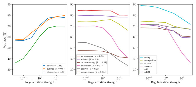
Figure 1: Effect of varying DKM regularization strength ($\nu$) on validation performance for homophilous node classification datasets (left), heterophilous node classification datasets (middle), and graph classification tasks (right). Validation accuracies were obtained by taking optimal settings from the grid search for the graph convolutional NNGP, and varying $\nu$.

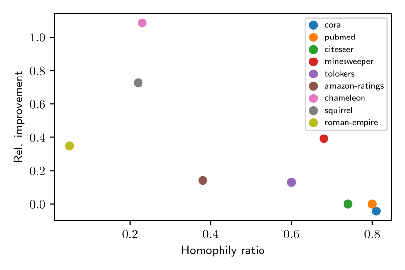
Figure 2: Effect of varying DKM regularization strength ($\nu$) on validation performance for homophilous node classification datasets (left), heterophilous node classification datasets (middle), and graph classification tasks (right). Relative improvement is calculated as the change in test error when changing from an NNGP to a DKM.

5.1 Overview

To empirically test the graph convolutional DKM, we benchmarked it against the graph convolutional NNGP and the GCN, on several node classification and graph classification datasets. We demonstrate that the flexible graph convolutional DKM is competitive with the GCN on all but one dataset, and that the fixed representation graph convolutional NNGP is competitive only when graphs are homophilous.

The experiments were conducted broadly on two types of dataset:

• Node classification datasets with a single graph. For the Planetoid datasets (Sen et al., 2008),  Cora, Citeseer, and Pubmed, the task is to predict scientific paper topics from citations; and the Squirrel and Chameleon tasks (Rozemberczki et al., 2021) are to predict daily traffic for Wikipedia pages related to the corresponding animals from their hyperlinks. The remaining node classification datasets were introduced by Platonov et al. (2023). The Roman Empire task is to syntactically classify words on the Roman Empire Wikipedia article based on syntactic and positional relationships; Minesweeper involves solving a game of minesweeper using a graphical representation of the grid; Amazon Ratings requires predicting user ratings of products; and the Tolokers dataset is about predicting whether users have been banned from the Tolokers platform, by using information about other users that have performed the same tasks.

• Graph classification datasets with multiple graphs (Morris et al., 2020). These are all molecule datasets with the molecules represented as graphs, where the task is to predict properties of the molecules. NCI1 and NCI109 are chemical compound datasets, Proteins and Enzymes are protein datasets, and Mutag and Mutagenicity are both datasets of compounds.

Appendix A.1 contains further qualitative details about the datasets, and Tables 1 and 2 show dataset summary statistics.

We measure homophily of a graph by homophily ratio, which is the ratio of the number of edges between ‘like nodes’ and the total number of nodes, where by ‘like nodes’ we mean nodes with the same label. We can calculate the homophily ratio for the node classification datasets, but not the graph classification datasets (because for these datasets we only have graph-level labels and not node labels). Cora, Citeseer and Pubmed are highly homophilous, with homophily ratios $>0.8$. The remaining node classification datasets all have homophily ratios $<0.7$. We expect graph classification datasets to exhibit both homophily and heterophily, because they are made up of molecules (Ye et al., 2022).

In our experiments, we used grid searches on each dataset to optimize hyperparameters. We trained a GCN in addition to the DKM and NNGP for the node classification datasets, where we used similar architectures for fair comparison. The most important hyperparameter for the DKM is the regularization $\nu$. Rather than having a different regularization at each layer as in Eq. 17, we set $\nu_{\ell}=\nu$, and for each dataset we perform a grid search over $\nu$. We optimized other hyperparameters such as number of layers, number of hidden units/inducing points, and more, details of which can be found in Appendix A.2.

5.2 Results

Tables 3 and 4 summarize accuracies on each dataset. Table 3 show that the graph convolutional DKM is competitive with the GCN on all node classification datasets with the exception of Roman Empire. One possible reason for the poor performance on Roman Empire is that the GCN was trained with dropout which boosts performance significantly, but we did not train the DKM with an analogous regularizer (specifically, we found that a GCN without dropout performed significantly worse during the grid search stage, with a mean validation accuracy of $77.0\%$ without dropout vs. $83.3\%$ with dropout). The performance of the graph convolutional NNGP is close on Cora, Citeseer, Pubmed, Tolokers, but significantly worse on all other datasets. Table 4 shows that the graph convolutional DKM is roughly comparable to the GCN on the graph classification tasks, whereas the graph convolutional NNGP is not comparable on any dataset.

Figure 1 summarizes the effect of DKM regularization ($\nu$) on performance for different datasets. When DKM regularization is higher, the model is regularized more towards the graph convolutional NNGP. We see on datasets with high homophily (Cora, Citeseer, Pubmed) that higher regularization is preferred, indicating that the fixed representations of the NNGP are sufficient to solve the task. The same cannot be said of the remaining datasets, which are not highly homophilous — performance degrades either marginally or significantly as we regularize more towards the NNGP ($\nu=\infty$).

Figure 2 shows the relationship between performance improvement and homophily ratio. The relationship is significant with t-value $-2.54$ (df=$7$) and p-value $0.04$. When the homophily ratio is high, we see that there is little improvement in switching from the fixed NNGP representations to the flexible DKM representations. Conversely, when the homophily ratio is low we see big gains. This suggests that the fixed representations of the NNGP are insufficient to explain data on heterophilous graphs.

6 Conclusion and Discussion

By leveraging the deep kernel machine framework, we have developed a flexible variant of an infinite-width graph convolutional network. The graph convolutional DKM provides a hyperparameter that allows us to interpolate between a flexible kernel machine and the graph convolutional NNGP with fixed kernel. This feature of the DKM enabled us to examine the importance of representation learning on graph tasks. Remarkably, we found that not all graph tasks benefit from representation learning. Moreover, we found that the importance of representation learning for a particular task correlates with the level of heterophily, with more heterophily requiring more flexibility. This finding helps explain the fact that NNGPs have previously been shown to perform well on graph tasks, but not in other domains such as images.

Despite using an inducing point scheme, computational cost of the graph DKMs is high. We expect that improving computational efficiency can help improve performance, as it would allow for easier architecture exploration, and training of bigger models. We also expect that more careful optimization could aid performance. However, we leave these issues for future work.

7 Impact Statement

This paper presents work whose goal is to advance the field of machine learning, and more specifically our understanding of representation learning in graphs. There are many potential societal consequences of our work, none which we feel must be specifically highlighted here.

Appendix A Experimental details

Our experiments involved benchmarking the graph convolutional DKM and a graph convolutional NNGP on several node and graph classification datasets. We also benchmarked a GCN on the same datasets to obtain a suitable baseline.

A.1 Dataset details

The datasets we benchmarked split broadly into two categories: node classification and graph classification. Statistics for each dataset are given in Tables 1 and 2, but here we describe the datasets qualitatively.

For the node classification datasets, the task is to predict the labels of all nodes in a single graph, given labels for only limited number of nodes. Cora, Citeseer, and Pubmed (Planetoid datasets) are all citation networks, where nodes represent scientific publications, and edges are citations between those publications; one-hot keyword encodings are provided as features, and the goal is to place documents into predefined categories. Chameleon and Squirrel are both Wikipedia networks on their respective topics, so that nodes correspond to articles, and edges correspond to links between articles; features are again one-hot as in the citation networks, but represent the presence of relevant nouns, and the task is to categories pages based on their average daily traffic. The remaining node classification datasets have unrelated domains, but were all introduced by Platonov et al. (2023):

• Roman Empire is derived entirely from the Roman Empire article on Wikipedia. Nodes are words in the text, and the words are ‘connected’ if they are either adjacent in a sentence or if they are dependent on each other syntactically. Features are word embeddings, and the task is to label each word’s syntactic role.

• Tolokers is a dataset of workers from the Toloka platform. The nodes are workers, and nodes are connected if workers have worked on the same task. Features are statistics about each worker, and the task is to predict if a worker has been banned.

• Minesweeper is a synthetic dataset. The graph has 10,000 nodes corresponding to the cells in the 100 by 100 grid in the Minesweeper game. Nodes are connected if the associated cells are adjacent. Features are one-hot encoded numbers of neighbouring mines, plus a extra feature for when the number of neighbouring mines is unknown. The task is to predict which nodes are mines.

• Amazon Ratings is a graph where nodes are Amazon products, and nodes are connected if they are commonly purchased together. Features are text embeddings of the product descriptions. The task is to predict the average user rating.

The graph classification datasets all contain molecules. NCI1 and NCI109 both contain graphs of chemical compounds (nodes representing atoms, and with nodes connected if there are chemical bonds between them), where the goal is to predict effect of the compounds vs. lung and ovarian cancer. Enzymes is a dataset of protein tertiary structures, and the task is to classify according to protein class. Proteins is a dataset of proteins, where the task is to classify as enzymes or non-enzymes. Mutag is a dataset of compounds, and the task is to predict mutagenicity on Salmonella typhimurium. Finally, Mutagenicity is a dataset of drug compounds, and the task is to categorize into mutagen or non-mutagen.

A.2 Details of training, hyperpameter selection and final benchmarking

For the node classification datasets, we used publicly available train/validation/test splits from the Pytorch Geometric library (Fey & Lenssen, 2019). For the graph classification datasets, we created train/test (90%/10%) splits using a stratified K-fold similarly to Balcilar et al. (2020); for hyperparameter selection, we further introduced a validation set by randomly selecting graphs from the train set to obtain a 80%/10%/10% split. For data preprocessing, we (a) renormalize all adjacency matrices as Kipf & Welling (2017), (b) add a node degree feature to the graph classification datasets, and (c) Z-scale node features in the Enzymes dataset.

Each node classification model was trained for 200 epochs using the Adam optimizer. We used a learning rate of $10^{-2}$ for the first 100 epochs, $10^{-3}$ for the next 50, $10^{-4}$ for the next 25, and $10^{-5}$ for the final 25 epochs. For the graph classification tasks we trained for 120 epochs, warming-up for 40 epochs from $10^{-3}$ to $10^{-2}$ and then halving every subsequent 20 epochs. For the planetoid datasets, we used the same 2-layer GCN architecture as Kipf & Welling (2017), but with batchnorm For the graph classification datasets, we also used the architecture from Kipf & Welling (2017), but with 6 layers. For the remaining datasets, we use the same GCN architecture as Platonov et al. (2023). When training the graph convolutional DKMs, we mirrored the GCN architectures — in place of linear layers we used Gram layers, in place of ReLU non-linearities we used the ReLU kernel non-linearity (Cho & Saul, 2009) with $\sigma_{b}=0$ and $\sigma_{w}=1$, in place of batchnorm, we used global kernel norm from Milsom et al. (2023).

To find suitable hyperparameters for the GCN, we used a grid search. When using the GCN architecture from Kipf & Welling (2017), we grid searched over number of hidden units $\in\{16,32,64,128\}$, dropout $\in\{0,0.5\}$, batchnorm $\in\{\text{yes},\text{no}\}$, and row normalizing features $\in\{\text{yes},\text{no}\}$. When using the architecture from Platonov et al. (2023), we do the same, except we search over hidden units $\in\{128,384\}$ and additionally number of layers $\in\{2,3,4\}$.

To find hyperparameters for the graph convolutional DKM in the node classification setting, we performed two separate grid searches. We searched for regularization $\nu\,\in\{0,10^{-3},10^{-2},10^{-1},10^{0},10^{1},10^{2},10^{3},\infty\}$. Once these settings had been obtained, we increased the number of inducing points from 128 to 512, and grid searched over different inducing Gram matrix initializations, and whether to learn a feature scaling in the input layer. For some datasets (e.g. Pubmed) we found it was necessary to use a random initialization rather than an NNGP initialization to ensure numerical stability. In the graph classification setting, we performed a single grid search over inducing points $P_{\mathrm{i}}\in\{128,256,384\}$, $\nu\in\{0,10^{-3},\ldots,10^{3},\infty\}$ and number of layers $\in\{2,4,6\}$.

For the final benchmark, we report the mean accuracies on the test sets. For the planetoid dataset, we averaged over 20 random seeds. The remaining datasets each have 10 splits — we perform 50 training runs, and report the mean accuracy over all of these runs.

The code was written in Pytorch, and we trained using Bristol’s Advanced Computing Research Centre (ACRC), on a cluster containing RTX 3090’s, and A100s.

A.3 Extended results

For completeness, we provide all of our GCN and graph convolutional NNGP results on the node classification datasets in Table 5, as in Table 3 we used the results of others where comparable results are available.

Table 5: Node classification test accuracies $\pm$ one standard deviation.

Dataset (homophily ratio)	Graph Conv. DKM	Graph Conv. NNGP	GCN
Roman Empire ($0.05$)	$75.6\pm 0.7$	$67.1\pm 0.4$	$83.4\pm 0.4$
Squirrel ($0.22$)	$57.7\pm 1.8$	$27.0\pm 1.7$	$58.5\pm 1.9$
Chameleon ($0.24$)	$70.8\pm 1.9$	$39.1\pm 3.0$	$67.8\pm 2.8$
Amazon Ratings ($0.38$)	$48.8\pm 0.6$	$41.6\pm 0.3$	$49.3\pm 0.6$
Tolokers ($0.6$)	$80.7\pm 0.6$	$78.2\pm 0.1$	$80.7\pm 0.3$
Minesweeper ($0.68$)	$85.7\pm 0.5$	$80.1\pm 0.1$	$86.6\pm 0.6$
Citeseer ($0.74)$	$69.5\pm 0.2$	$69.5\pm 0.2$	$70.0\pm 0.2$
Pubmed ($0.8$)	$79.4\pm 0.1$	$79.4\pm 0.1$	$78.1\pm 0.3$
Cora ($0.81$)	$81.5\pm 0.2$	$82.3\pm 0.1$	$81.2\pm 0.3$

Appendix B Inducing Point Approximation

B.1 Sparse Deep Kernel Machines

Sparse DKMs are inspired by the sparse DGP literature (Damianou & Lawrence, 2013; Salimbeni & Deisenroth, 2017), where the variational inference (VI) framework is used. One can obtain a sparse DKM by using an approximate posterior that introduces inducing features ${\bm{\mathbf{F}}}_{\mathrm{i}}^{\ell}\in\mathbb{R}^{P_{\mathrm{i}}\times N_{\ell}}$ in addition to the ‘real’ test/training features ${\bm{\mathbf{F}}}_{\mathrm{t}}^{\ell}\in\mathbb{R}^{P_{\mathrm{t}}\times N_{\ell}}$, at each layer in the DGP (Eq. 1). The implied Gram matrices (and kernels) are similarly split into “inducing-inducing” ($\mathrm{ii}$), “test/train-test/train” ($\mathrm{tt}$), and “inducing-test/train” ($\mathrm{it}$/$\mathrm{ti}$) blocks:

$$\mathbf{G}^{\ell}=\mathbf{F}^{\ell}(\mathbf{F}^{\ell})^{T}=\begin{pmatrix}{\bm{\mathbf{F}}}_{\mathrm{i}}^{\ell}\\ {\bm{\mathbf{F}}}_{\mathrm{t}}^{\ell}\end{pmatrix}\begin{pmatrix}{\bm{\mathbf{F}}}_{\mathrm{i}}^{\ell}\\ {\bm{\mathbf{F}}}_{\mathrm{t}}^{\ell}\end{pmatrix}^{T}=\begin{pmatrix}{\bm{\mathbf{F}}}_{\mathrm{i}}^{\ell}({\bm{\mathbf{F}}}_{\mathrm{i}}^{\ell})^{T}&{\bm{\mathbf{F}}}_{\mathrm{i}}^{\ell}({\bm{\mathbf{F}}}_{\mathrm{t}}^{\ell})^{T}\\ {\bm{\mathbf{F}}}_{\mathrm{t}}^{\ell}({\bm{\mathbf{F}}}_{\mathrm{i}}^{\ell})^{T}&{\bm{\mathbf{F}}}_{\mathrm{t}}^{\ell}({\bm{\mathbf{F}}}_{\mathrm{t}}^{\ell})^{T}\end{pmatrix}=\begin{pmatrix}\mathbf{G}_{\text{ii}}^{\ell}&(\mathbf{G}_{\text{ti}}^{\ell})^{T}\\ \mathbf{G}_{\text{ti}}^{\ell}&\mathbf{G}_{\text{tt}}^{\ell}\end{pmatrix}$$ (18)

This approximate posterior results in (see Yang et al. (2023) for details) the following evidence lower bound (ELBO), sometimes called the “sparse DKM objective”:

$$\begin{split}\mathcal{L}_{\text{sparse}}(\mathbf{G}_{\text{ii}}^{1},\dots,\mathbf{G}_{\text{ii}}^{L},\bm{\mu}_{1},\dots,\bm{\mu}_{\nu_{L+1}},\bm{\Sigma})=&\;\text{GP-ELBO}(\mathbf{Y}\mid\mathbf{G}^{L},\bm{\mu}_{1},\dots,\bm{\mu}_{\nu_{L+1}},\bm{\Sigma})\\ &-\sum_{\ell=1}^{L}\nu_{\ell}\mathrm{D}_{\mathrm{KL}}\left(\mathcal{N}(\bm{\mathbf{0}},\bm{\mathbf{G}}_{\text{ii}}^{\ell})\mid\mid\mathcal{N}(\bm{\mathbf{0}},\bm{\mathbf{K}}(\bm{\mathbf{G}}_{\text{ii}}^{\ell-1}))\right).\end{split}$$ (19)

Here, GP-ELBO is the ELBO of a (shallow) sparse GP fitted on labels $\mathbf{Y}$. The GP prior is zero-mean and has kernel $\mathbf{K}(\mathbf{G}^{L})$, and we use an approximate posterior $\mathcal{N}(\bm{\mu}_{\lambda},\bm{\Sigma}_{\lambda}$) over each inducing output feature $\lambda=1,\dots,\nu_{L+1}$. We share a single covariance matrix $\bm{\Sigma}_{\lambda}=\bm{\Sigma}$ across all output features to reduce computational cost. As usual in variational inference, we optimise hyperparameters, such as the inducing input locations $\mathbf{X}_{\text{i}}$ or kernel-specific hyperparameters, using this same objective.

B.2 Sparse graph convolutional DKMs

In the graph convolutional DKM, we take our inducing points to be completely isolated inducing nodes, in the sense that they are neither adjacent to other inducing points, nor test/train nodes. Concretely, the graph convolutional NNGP kernel matrix (Eq. 15), when using the sparse inducing point scheme, becomes a block matrix as in Eq. 18, with blocks

$$\mathbf{K}_{\text{GCN}}(\mathbf{G}^{\ell-1})=\begin{pmatrix}\bm{\mathbf{\Phi}}_{\text{ii}}({\bm{\mathbf{G}}}_{\mathrm{ii}}^{\ell-1})&\bm{\mathbf{\Phi}}_{\text{it}}(\bm{\mathbf{G}}^{\ell-1})\hat{\bm{\mathbf{A}}}^{T}\\ \hat{\bm{\mathbf{A}}}\bm{\mathbf{\Phi}}_{\text{ti}}(\bm{\mathbf{G}}^{\ell-1})&\hat{\bm{\mathbf{A}}}\bm{\mathbf{\Phi}}_{\text{tt}}({\bm{\mathbf{G}}}_{\mathrm{tt}}^{\ell-1})\hat{\bm{\mathbf{A}}}^{T}\end{pmatrix}.$$ (20)

where $\bm{\mathbf{\Phi}}_{\text{ii}},\bm{\mathbf{\Phi}}_{\text{ti}},\bm{\mathbf{\Phi}}_{\text{tt}}$ refer to the blocks of the kernel matrix resulting from applying the “base kernel” (e.g. the arccos kernel) to $\bm{\mathbf{G}}^{\ell-1}$. The full derivation is given in Appendix C. This inducing point scheme can be used for datasets with a single graph or multiple graphs. In the case where the dataset is a single graph, we use a minibatch size of 1, and the ‘minibatch’ becomes all nodes in the graph. In the case where the dataset contains several graphs, the graphs can be batched together. Naively, this would involve creating a single large adjacency matrix that describes adjacency information for graphs in the minibatch, but in practice this can be efficiently represented with a sparse tensor.

B.3 Improving computational complexity with a Nyström approximation

Section B.2 describes how to avoid an $\mathcal{O}(P^{3})$ time complexity by using inducing point scheme, but the test/train Gram matrices ${\bm{\mathbf{G}}}_{\mathrm{tt}}$ are still a computational bottleneck. Specifically, storing covariances between nodes is expensive because it involves calculating and storing a node-by-node matrix, which is prohibitively costly for large graphs. We don’t have this problem with adjacency matrices, because they can often be assumed to be sparse. However, there is no reason to assume that covariance matrices are sparse, so a similar trick cannot be applied for efficiently storing ${\bm{\mathbf{G}}}_{\mathrm{tt}}$.

We can resolve this issue by propagating only the diagonal of ${\bm{\mathbf{G}}}_{\mathrm{tt}}^{\ell}$ through the DKM. This is feasible in the output layer because we only need the diagonal at the output layer (since the DKM model assumes an IID distribution over output features). When performing the graph convolution in a graph convolutional DKM, we still need to propagate the diagonal of $\hat{\bm{\mathbf{A}}}\bm{\mathbf{\Phi}}_{\mathrm{tt}}\hat{\bm{\mathbf{A}}}^{T}$, which usually requires the full coavariance $\bm{\mathbf{\Phi}}_{\mathrm{tt}}$, but this can be avoided by using a Nyström approximation:

$$\bm{\mathbf{\Phi}}_{\mathrm{tt}}\approx\bm{\mathbf{\Phi}}_{\mathrm{ti}}\bm{\mathbf{\Phi}}_{\mathrm{ii}}^{-1}\bm{\mathbf{\Phi}}_{\mathrm{it}}+\bm{\mathbf{D}}.$$ (21)

Here, $\bm{\mathbf{D}}$ is a diagonal correction, since we know the true diagonal. The graph convolution operation then becomes $\bm{\mathbf{K}}_{\mathrm{tt}}\approx\hat{\bm{\mathbf{A}}}(\bm{\mathbf{\Phi}}_{\mathrm{ti}}\bm{\mathbf{\Phi}}_{\mathrm{ii}}^{-1}\bm{\mathbf{\Phi}}_{\mathrm{it}}+\bm{\mathbf{D}})\hat{\bm{\mathbf{A}}}^{T}$, and since we only need the diagonal, this can be computed efficiently when $\hat{\bm{\mathbf{A}}}$ is sparse using the following identity,

$$\mathrm{diag}(\hat{\bm{\mathbf{A}}}(\bm{\mathbf{\Phi}}_{\mathrm{ti}}\bm{\mathbf{\Phi}}_{\mathrm{ii}}^{-1}\bm{\mathbf{\Phi}}_{\mathrm{it}}+\bm{\mathbf{D}})\hat{\bm{\mathbf{A}}}^{T})=\mathrm{colsum}(\bm{\mathbf{K}}_{\mathrm{ti}}\bm{\mathbf{\Phi}}_{\mathrm{ii}}^{-1}\odot\bm{\mathbf{K}}_{\mathrm{ti}})+\mathrm{colsum}(\hat{\bm{\mathbf{A}}}\odot\hat{\bm{\mathbf{A}}}\odot_{\mathrm{b}}\mathrm{diag}(\bm{\mathbf{D}})),$$ (22)

where $\odot$ is the pointwise Hadamard product, and $(\hat{\bm{\mathbf{A}}}\odot_{\mathrm{b}}\mathrm{diag}(\bm{\mathbf{D}}))_{ij}=\hat{\bm{\mathbf{A}}}_{ij}\mathrm{diag}(\bm{\mathbf{D}})_{j}$ is the ‘broadcasted’ pointwise multiplication of the diagonal correction with each column of $\hat{\bm{\mathbf{A}}}$.

With this Nyström approximation, the memory cost for the forward pass is in theory $\mathcal{O}(P_{\mathrm{t}}P_{\mathrm{i}})$, and the time complexity is $\mathcal{O}(LP_{\mathrm{t}}P_{\mathrm{i}}\mathopen{|}\mathcal{E}\mathclose{|})$ where $L$ is the number of layers and $\mathopen{|}\mathcal{E}\mathclose{|}$ is the number of edges in the graph. Unfortunately, due to lack of support in PyTorch for sparse tensors, we don’t implement Eq. 22 for our experiments. Instead, while we do use the Nyström approximation, we resort to computing the full test/train covariance matrices with Eq. 21.

The complete graph convolutional DKM prediction algorithm is given in Algorithm 1. The prediction algorithm as presented is for node regression problems. It can be modified to allow for classification problems by treating the Gaussian outputs as logits. We can also modify the algorithm for graph level problems (e.g. graph classification) by applying global average pooling to the final kernel, $\bm{\mathbf{K}}(\bm{\mathbf{G}}^{L})$.

Algorithm 1 DKM prediction for node regression

  Parameters: $\{\nu_{\ell}\}_{\ell=1}^{L}$

  Inducing Gram matrices: $\{{\bm{\mathbf{G}}}^{\ell}_{\mathrm{ii}}\}_{\ell=1}^{L+1}$

  Inducing and train/test inputs: ${\bm{\mathbf{X}}}_{\mathrm{i}}$, ${\bm{\mathbf{X}}}_{\mathrm{t}}$

  Inducing outputs variational parameters: $\bm{\mu}_{1},\dots,\bm{\mu}_{\nu_{L+1}},\bm{\Sigma}$

  Initialize full Gram matrix

  $\begin{pmatrix}{\bm{\mathbf{G}}}^{0}_{\mathrm{ii}}&{\bm{\mathbf{G}}}^{0}_{\mathrm{it}}\\ {\bm{\mathbf{G}}}^{0}_{\mathrm{ti}}&{\bm{\mathbf{G}}}^{0}_{\mathrm{tt}}\end{pmatrix}\leftarrow\frac{1}{\nu_{0}}\begin{pmatrix}{\bm{\mathbf{X}}}_{\mathrm{i}}{\bm{\mathbf{X}}}_{\mathrm{i}}^{T}&{\bm{\mathbf{X}}}_{\mathrm{i}}{\bm{\mathbf{X}}}_{\mathrm{t}}^{T}\\ {\bm{\mathbf{X}}}_{\mathrm{t}}{\bm{\mathbf{X}}}_{\mathrm{i}}^{T}&{\bm{\mathbf{X}}}_{\mathrm{t}}{\bm{\mathbf{X}}}_{\mathrm{t}}^{T}\end{pmatrix}$

  for $\ell$ in $(1,\dotsc,L)$ do

     Apply kernel non-linearity

     $\begin{pmatrix}{\bm{\mathbf{\Phi}}}^{\ell}_{\mathrm{ii}}&{\bm{\mathbf{\Phi}}}^{\ell}_{\mathrm{it}}\\ {\bm{\mathbf{\Phi}}}^{\ell}_{\mathrm{ti}}&{\bm{\mathbf{\Phi}}}^{\ell}_{\mathrm{tt}}\end{pmatrix}\leftarrow{\bm{\mathbf{\Phi}}}\left({\begin{pmatrix}{\bm{\mathbf{G}}}^{\ell-1}_{\mathrm{ii}}&{\bm{\mathbf{G}}}^{\ell-1}_{\mathrm{it}}\\ {\bm{\mathbf{G}}}^{\ell-1}_{\mathrm{ti}}&{\bm{\mathbf{G}}}^{\ell-1}_{\mathrm{tt}}\end{pmatrix}}\right)$

     Perform graph convolution

     ${\bm{\mathbf{K}}}_{\mathrm{ii}}\leftarrow{\bm{\mathbf{\Phi}}}^{\ell}_{\mathrm{ii}}$

     ${\bm{\mathbf{K}}}_{\mathrm{ti}}\leftarrow{\hat{\bm{\mathbf{A}}}}{\bm{\mathbf{\Phi}}}^{\ell}_{\mathrm{ti}}$

     ${\bm{\mathbf{K}}}_{\mathrm{tt}}\leftarrow{\hat{\bm{\mathbf{A}}}}{\bm{\mathbf{\Phi}}}^{\ell}_{\mathrm{tt}}{\hat{\bm{\mathbf{A}}}}^{T}$ (or use Nyström approximation from Section B.3)

     Propagate the test-test and test-inducing blocks, using conditional Gaussian formulae (Yang et al., 2023)

     ${\bm{\mathbf{K}}}_{\mathrm{tt}\cdot\mathrm{i}}\leftarrow{\bm{\mathbf{K}}}_{\mathrm{tt}}-{\bm{\mathbf{K}}}_{\mathrm{ti}}{\bm{\mathbf{K}}}_{\mathrm{ii}}^{-1}{\bm{\mathbf{K}}}_{\mathrm{it}}.$

     ${\bm{\mathbf{G}}}_{\mathrm{ti}}^{\ell}\leftarrow{\bm{\mathbf{K}}}_{\mathrm{ti}}{\bm{\mathbf{K}}}_{\mathrm{ii}}^{-1}{\bm{\mathbf{G}}}^{\ell}_{\mathrm{ii}}$

     ${\bm{\mathbf{G}}}_{\mathrm{tt}}^{\ell}\leftarrow{\bm{\mathbf{K}}}_{\mathrm{ti}}{\bm{\mathbf{K}}}_{\mathrm{ii}}^{-1}{\bm{\mathbf{G}}}^{\ell}_{\mathrm{ii}}{\bm{\mathbf{K}}}_{\mathrm{ii}}^{-1}{\bm{\mathbf{K}}}_{\mathrm{it}}+{\bm{\mathbf{K}}}_{\mathrm{tt}\cdot\mathrm{i}}$

  end for

  Output layer ($L+1$) prediction using standard sparse Gaussian process expressions

  $\begin{pmatrix}{\bm{\mathbf{K}}}^{L+1}_{\mathrm{ii}}&{\bm{\mathbf{K}}}^{L+1}_{\mathrm{it}}\\ {\bm{\mathbf{K}}}^{L+1}_{\mathrm{ti}}&{\bm{\mathbf{K}}}^{L+1}_{\mathrm{tt}}\end{pmatrix}\leftarrow{\bm{\mathbf{\Phi}}}{\left(\begin{pmatrix}{\bm{\mathbf{G}}}^{L}_{\mathrm{ii}}&{\bm{\mathbf{G}}}^{L}_{\mathrm{it}}\\ {\bm{\mathbf{G}}}^{L}_{\mathrm{ti}}&{\bm{\mathbf{G}}}^{L}_{\mathrm{tt}}\end{pmatrix}\right)}$

  $\bm{\mathbf{m}}_{\lambda}\leftarrow{\bm{\mathbf{K}}}_{\mathrm{ti}}^{L+1}({\bm{\mathbf{K}}}_{\mathrm{ii}}^{L+1})^{-1}{\bm{\mathbf{\mu}}_{\lambda}}$

  ${\bm{\mathbf{G}}}_{\mathrm{tt}}^{L+1}\leftarrow{\bm{\mathbf{K}}}_{\mathrm{tt}}^{L+1}-{\bm{\mathbf{K}}}_{\mathrm{ti}}^{L+1}({\bm{\mathbf{K}}}_{\mathrm{ii}}^{L+1})^{-1}{\bm{\mathbf{K}}}_{\mathrm{it}}^{L+1}+{\bm{\mathbf{K}}}_{\mathrm{ti}}^{L+1}({\bm{\mathbf{K}}}_{\mathrm{ii}}^{L+1})^{-1}\bm{\Sigma}({\bm{\mathbf{K}}}_{\mathrm{ii}}^{L+1})^{-1}{\bm{\mathbf{K}}}_{\mathrm{it}}^{L+1}$

  Generate samples of latent outputs ${\bm{\mathbf{F}}}_{\mathrm{t}}^{L+1}=(\bm{\mathbf{f}}_{1}^{\text{t;L+1}}\cdots\bm{\mathbf{f}}_{\nu_{L+1}}^{\text{t;L+1}})$ using variational distribution

  $\operatorname{Q}(\bm{\mathbf{f}}_{\lambda}^{\text{t;L+1}})\sim_{\text{ind}}\mathcal{N}\left(\bm{\mathbf{m}}_{\lambda},{\bm{\mathbf{G}}}_{\mathrm{tt}}^{L+1}\right)$

  regularizer $\leftarrow-\sum_{\ell=1}^{L}\nu_{\ell}\mathrm{D}_{\mathrm{KL}}\left(\mathcal{N}(\bm{\mathbf{0}},{\bm{\mathbf{G}}}_{\mathrm{ii}}^{\ell})\mid\mid\mathcal{N}(\bm{\mathbf{0}},{\bm{\mathbf{K}}}_{\mathrm{ii}}^{\ell})\right)$

  likelihood_lb $\leftarrow\mathbb{E}_{\operatorname{Q}({\bm{\mathbf{F}}}_{\mathrm{t}}^{L+1})}[\operatorname{P}(\bm{\mathbf{Y}}_{\mathrm{t}}\mid{\bm{\mathbf{F}}}_{\mathrm{t}}^{L+1})]-\sum_{\lambda=1}^{N_{L+1}}\mathrm{D}_{\mathrm{KL}}\left(\mathcal{N}(\bm{\mathbf{f}}^{L+1}_{\lambda},\bm{\mathbf{\Sigma}})\mid\mid\mathcal{N}(\bm{\mathbf{0}},{\bm{\mathbf{K}}}_{\mathrm{ii}}^{L+1})\right)$

  $\mathcal{L}_{\mathrm{LB}}\leftarrow\texttt{likelihood\_lb}+\texttt{regularizer}$

  output $\leftarrow\operatorname{Q}({\bm{\mathbf{F}}}_{\mathrm{t}}^{L+1}),\,\mathcal{L}_{\mathrm{LB}}$

Appendix C Graph convolutional NNGP kernel derivations

In this appendix we show how to derive the kernel/covariance expressions given in Eq. 15 (for the full-rank case) and Eq. 20 (for the sparse inducing point case).

With the “completely isolated” inducing nodes described in the main text, the pre-activation features $\mathbf{F}^{\ell}_{\text{i}},\mathbf{F}^{\ell}_{\text{t}}$ for the inducing and test/train blocks are given by the following, in suffix notation:

$$F^{\text{i};\ell}_{i\lambda} =\sum_{\mu}H^{\text{i};\ell-1}_{i\mu}W_{\mu\lambda}$$ (23)

$$F^{\text{t};\ell}_{s\lambda} =\sum_{s^{\prime}\mu}\hat{A}_{ss^{\prime}}H^{\text{t};\ell-1}_{s^{\prime}\mu}W_{\mu\lambda}$$ (24)

and we wish to compute the covariances between features as our kernel, i.e.

$$\begin{pmatrix}{\bm{\mathbf{K}}}_{\mathrm{ii}}&{\bm{\mathbf{K}}}_{\mathrm{it}}\\ {\bm{\mathbf{K}}}_{\mathrm{ti}}&{\bm{\mathbf{K}}}_{\mathrm{tt}}\end{pmatrix}=\begin{pmatrix}\mathbb{E}[\mathbf{f}^{\text{i};\ell}_{\lambda}(\mathbf{f}^{\text{i};\ell}_{\lambda})^{T}]&\mathbb{E}[\mathbf{f}^{\text{i};\ell}_{\lambda}(\mathbf{f}^{\text{t};\ell}_{\lambda})^{T}]\\ \mathbb{E}[\mathbf{f}^{\text{t};\ell}_{\lambda}(\mathbf{f}^{\text{i};\ell}_{\lambda})^{T}]&\mathbb{E}[\mathbf{f}^{\text{t};\ell}_{\lambda}(\mathbf{f}^{\text{t};\ell}_{\lambda})^{T}]\end{pmatrix}$$ (25)

where we need only consider one feature $\lambda$ since the features are IID over $\lambda\in\{1,\dots,N_{\ell}\}$.

For the inducing block, we have

$$K^{\text{ii};\ell}_{ij} =\mathbb{E}\left[F^{\text{i};\ell}_{i,\lambda}F^{\text{i};\ell}_{j,\lambda}\right]$$ (26)

$$=\mathbb{E}\left[\sum_{\mu}H^{\text{i};\ell-1}_{i\mu}W^{\ell}_{\mu\lambda}\sum_{\nu}H^{\text{i};\ell-1}_{j\nu}W^{\ell}_{\nu\lambda}\right]$$ (27)

$$=\sum_{\mu\nu}H^{\text{i};\ell-1}_{i\mu}H^{\text{i};\ell-1}_{j\nu}\mathbb{E}\left[W^{\ell}_{\mu\lambda}W^{\ell}_{\nu\lambda}\right]$$ (28)

$$=\tfrac{1}{N_{\ell-1}}\sum_{\mu\nu}H^{\text{i};\ell-1}_{i\mu}H^{\text{i};\ell-1}_{j\nu}\delta_{\mu,\nu}$$ (29)

$$=\tfrac{1}{N_{\ell-1}}\sum_{\mu}H^{\text{i};\ell-1}_{i\mu}H^{\text{i};\ell-1}_{j\mu}$$ (30)

$$=\Phi^{\text{ii};\ell-1}_{ij}$$ (31)

$$\text{so }{\bm{\mathbf{K}}}_{\mathrm{ii}}^{\ell}({\bm{\mathbf{G}}}_{\mathrm{ii}}^{\ell-1}) =\bm{\mathbf{\Phi}}({\bm{\mathbf{G}}}_{\mathrm{ii}}^{\ell-1})$$ (32)

where $\bm{\mathbf{\Phi}}(\cdot)$ is the kernel function associated with the neural network non-linearity, e.g. an arccos kernel (Cho & Saul, 2009) in the case of a ReLU non-linearity. Hence the inducing-inducing block of the kernel matrix acts just like in the original “fully-connected” DKM (Yang et al., 2023).

For the inducing-test/train block, we have

$$K^{\text{it};\ell}_{is} =\mathbb{E}\left[F^{\text{i};\ell}_{i,\lambda}F^{\text{t};\ell}_{s,\lambda}\right]$$ (33)

$$=\mathbb{E}\left[\sum_{\mu}H^{\text{i};\ell-1}_{i\mu}W^{\ell}_{\mu\lambda}\sum_{\nu s^{\prime}}\hat{A}_{ss^{\prime}}H^{\ell-1}_{s^{\prime}\nu}W^{\ell}_{\nu\lambda}\right]$$ (34)

$$=\sum_{\mu\nu s^{\prime}}H^{\text{i};\ell-1}_{i\mu}\hat{A}_{ss^{\prime}}H^{\text{t};\ell-1}_{s^{\prime}\nu}\;\mathbb{E}\left[W^{\ell}_{\mu,\lambda}W^{\ell}_{\nu,\lambda}\right]$$ (35)

$$=\tfrac{1}{N_{\ell-1}}\sum_{\mu\nu s^{\prime}}H^{\text{i};\ell-1}_{i\mu}\hat{A}_{ss^{\prime}}H^{\text{t};\ell-1}_{s^{\prime}\nu}\delta_{\mu,\nu}$$ (36)

$$=\tfrac{1}{N_{\ell-1}}\sum_{\mu s^{\prime}}H^{\text{i};\ell-1}_{i\mu}\hat{A}_{ss^{\prime}}H^{\text{t};\ell-1}_{s^{\prime}\mu}$$ (37)

$$=\sum_{s^{\prime}}\Phi_{is^{\prime}}^{\text{it};\ell-1}\hat{A}_{ss^{\prime}}$$ (38)

$$\text{so }{\bm{\mathbf{K}}}_{\mathrm{it}}^{\ell}({\bm{\mathbf{G}}}_{\mathrm{it}}^{\ell-1}) =\bm{\mathbf{\Phi}}({\bm{\mathbf{G}}}_{\mathrm{it}}^{\ell-1})\mathbf{\hat{A}}^{T}.$$ (39)

Since the kernel is symmetric, ${\bm{\mathbf{K}}}_{\mathrm{ti}}={\bm{\mathbf{K}}}_{\mathrm{it}}^{T}$.

Finally, the test/train-test/train block is, in our isolated inducing nodes scheme, exactly the same as the full-rank case, which is given by

$$K^{\text{tt};\ell}_{sr} =\mathbb{E}\left[F^{\text{t};\ell}_{s\lambda}F^{\text{t};\ell}_{r\lambda}\right]$$ (40)

$$=\mathbb{E}\left[\sum_{\mu s^{\prime}}\hat{A}_{ss^{\prime}}H_{s\mu}^{\text{t};\ell-1}W^{\ell}_{\mu\lambda}\sum_{\nu r^{\prime}}\hat{A}_{rr^{\prime}}H_{r\nu}^{\text{t};\ell-1}W^{\ell}_{\nu\lambda}\right]$$ (41)

$$=\sum_{\mu\nu s^{\prime}r^{\prime}}\hat{A}_{ss^{\prime}}H^{\text{t};\ell-1}_{s\mu}\hat{A}_{rr^{\prime}}H^{\text{t};\ell-1}_{r\nu}\mathbb{E}\left[W^{\ell}_{\mu\lambda}W^{\ell}_{\nu\lambda}\right]$$ (42)

$$=\tfrac{1}{N_{\ell-1}}\sum_{\mu\nu s^{\prime}r^{\prime}}\hat{A}_{ss^{\prime}}H^{\text{t};\ell-1}_{s\mu}\hat{A}_{rr^{\prime}}H^{\text{t};\ell-1}_{r\nu}\delta_{\mu,\nu}$$ (43)

$$=\tfrac{1}{N_{\ell-1}}\sum_{\mu s^{\prime}r^{\prime}}\hat{A}_{ss^{\prime}}H^{\text{t};\ell-1}_{s\mu}\hat{A}_{rr^{\prime}}H^{\text{t};\ell-1}_{r\nu}$$ (44)

$$=\sum_{s^{\prime}r^{\prime}}\hat{A}_{ss^{\prime}}\Phi^{\text{tt};\ell-1}_{s^{\prime}r^{\prime}}\hat{A}_{rr^{\prime}}$$ (45)

$$\text{so }{\bm{\mathbf{K}}}_{\mathrm{tt}}^{\ell}({\bm{\mathbf{G}}}_{\mathrm{tt}}^{\ell-1}) =\mathbf{\hat{A}}\bm{\mathbf{\Phi}}({\bm{\mathbf{G}}}_{\mathrm{tt}}^{\ell-1})\mathbf{\hat{A}}^{T}.$$ (46)

References

- Achten et al. (2023) Achten, S., Tonin, F., Patrinos, P., and Suykens, J. A. Semi-supervised classification with graph convolutional kernel machines. arXiv preprint arXiv:2301.13764, 2023.
- Adlam et al. (2023) Adlam, B., Lee, J., Padhy, S., Nado, Z., and Snoek, J. Kernel regression with infinite-width neural networks on millions of examples. arXiv preprint arXiv:2303.05420, 2023.
- Aitchison (2020) Aitchison, L. Why bigger is not always better: on finite and infinite neural networks. In ICML, 2020.
- Balcilar et al. (2020) Balcilar, M., Renton, G., Héroux, P., Gauzere, B., Adam, S., and Honeine, P. Bridging the gap between spectral and spatial domains in graph neural networks. arXiv preprint arXiv:2003.11702, 2020.
- Bengio et al. (2013) Bengio, Y., Courville, A., and Vincent, P. Representation learning: A review and new perspectives. IEEE transactions on pattern analysis and machine intelligence, 35(8):1798–1828, 2013.
- Bordelon & Pehlevan (2023) Bordelon, B. and Pehlevan, C. Self-consistent dynamical field theory of kernel evolution in wide neural networks. Journal of Statistical Mechanics: Theory and Experiment, 2023(11):114009, 2023.
- Bronstein et al. (2017) Bronstein, M. M., Bruna, J., LeCun, Y., Szlam, A., and Vandergheynst, P. Geometric deep learning: going beyond euclidean data. IEEE Signal Processing Magazine, 34(4):18–42, 2017.
- Cho & Saul (2009) Cho, Y. and Saul, L. Kernel methods for deep learning. Advances in neural information processing systems, 2009.
- Cosmo et al. (2021) Cosmo, L., Minello, G., Bronstein, M., Rodolà, E., Rossi, L., and Torsello, A. Graph kernel neural networks. arXiv preprint arXiv:2112.07436, 2021.
- Damianou & Lawrence (2013) Damianou, A. and Lawrence, N. Deep gaussian processes. In Artificial Intelligence and Statistics, 2013.
- Fey & Lenssen (2019) Fey, M. and Lenssen, J. E. Fast graph representation learning with PyTorch Geometric. In ICLR Workshop on Representation Learning on Graphs and Manifolds, 2019.
- Garriga-Alonso et al. (2018) Garriga-Alonso, A., Rasmussen, C. E., and Aitchison, L. Deep convolutional networks as shallow gaussian processes. arXiv preprint arXiv:1808.05587, 2018.
- Hu et al. (2020) Hu, J., Shen, J., Yang, B., and Shao, L. Infinitely wide graph convolutional networks: semi-supervised learning via gaussian processes. arXiv preprint arXiv:2002.12168, 2020.
- Jacot et al. (2018) Jacot, A., Hongler, C., and Gabriel, F. Neural tangent kernel: Convergence and generalization in neural networks. In NeurIPS, pp. 8580–8589, 2018.
- Kashima et al. (2003) Kashima, H., Tsuda, K., and Inokuchi, A. Marginalized kernels between labeled graphs. In Proceedings of the 20th international conference on machine learning (ICML-03), pp. 321–328, 2003.
- Kipf & Welling (2017) Kipf, T. N. and Welling, M. Semi-supervised classification with graph convolutional networks. International Conference on Learning Representations, 2017.
- LeCun et al. (2015) LeCun, Y., Bengio, Y., and Hinton, G. Deep learning. nature, 521(7553):436–444, 2015.
- Lee et al. (2018) Lee, J., Bahri, Y., Novak, R., Schoenholz, S. S., Pennington, J., and Sohl-Dickstein, J. Deep neural networks as gaussian processes. International Conference on Learning Representations, 2018.
- Lee et al. (2020) Lee, J., Schoenholz, S., Pennington, J., Adlam, B., Xiao, L., Novak, R., and Sohl-Dickstein, J. Finite versus infinite neural networks: an empirical study. Advances in Neural Information Processing Systems, 33:15156–15172, 2020.
- MacKay et al. (1998) MacKay, D. J. et al. Introduction to gaussian processes. NATO ASI series F computer and systems sciences, 168:133–166, 1998.
- Matthews et al. (2018) Matthews, A. G. d. G., Rowland, M., Hron, J., Turner, R. E., and Ghahramani, Z. Gaussian process behaviour in wide deep neural networks. arXiv preprint arXiv:1804.11271, 2018.
- Milsom et al. (2023) Milsom, E., Anson, B., and Aitchison, L. Convolutional deep kernel machines, 2023.
- Morris et al. (2020) Morris, C., Kriege, N. M., Bause, F., Kersting, K., Mutzel, P., and Neumann, M. Tudataset: A collection of benchmark datasets for learning with graphs. arXiv preprint arXiv:2007.08663, 2020.
- Neal (1996) Neal, R. M. Bayesian Learning for Neural Networks, Vol. 118 of Lecture Notes in Statistics. Springer-Verlag, 1996.
- Niu et al. (2023) Niu, Z., Anitescu, M., and Chen, J. Graph neural network-inspired kernels for gaussian processes in semi-supervised learning. arXiv preprint arXiv:2302.05828, 2023. In press.
- Novak et al. (2018) Novak, R., Xiao, L., Lee, J., Bahri, Y., Yang, G., Hron, J., Abolafia, D. A., Pennington, J., and Sohl-Dickstein, J. Bayesian deep convolutional networks with many channels are gaussian processes. arXiv preprint arXiv:1810.05148, 2018.
- Platonov et al. (2023) Platonov, O., Kuznedelev, D., Diskin, M., Babenko, A., and Prokhorenkova, L. A critical look at the evaluation of gnns under heterophily: are we really making progress? arXiv preprint arXiv:2302.11640, 2023.
- Rozemberczki et al. (2021) Rozemberczki, B., Allen, C., and Sarkar, R. Multi-scale attributed node embedding. Journal of Complex Networks, 9(2):cnab014, 2021.
- Salimbeni & Deisenroth (2017) Salimbeni, H. and Deisenroth, M. Doubly stochastic variational inference for deep gaussian processes. Advances in neural information processing systems, 2017.
- Scarselli et al. (2008) Scarselli, F., Gori, M., Tsoi, A. C., Hagenbuchner, M., and Monfardini, G. The graph neural network model. IEEE transactions on neural networks, 20(1):61–80, 2008.
- Sen et al. (2008) Sen, P., Namata, G., Bilgic, M., Getoor, L., Galligher, B., and Eliassi-Rad, T. Collective classification in network data. AI magazine, 2008.
- Shankar et al. (2020) Shankar, V., Fang, A., Guo, W., Fridovich-Keil, S., Ragan-Kelley, J., Schmidt, L., and Recht, B. Neural kernels without tangents. In International conference on machine learning, pp. 8614–8623. PMLR, 2020.
- Shervashidze & Borgwardt (2009) Shervashidze, N. and Borgwardt, K. Fast subtree kernels on graphs. Advances in neural information processing systems, 22, 2009.
- Shervashidze et al. (2009) Shervashidze, N., Vishwanathan, S., Petri, T., Mehlhorn, K., and Borgwardt, K. Efficient graphlet kernels for large graph comparison. In Artificial intelligence and statistics, pp. 488–495. PMLR, 2009.
- Velicković et al. (2017) Velicković, P., Cucurull, G., Casanova, A., Romero, A., Lio, P., and Bengio, Y. Graph attention networks. arXiv preprint arXiv:1710.10903, 2017.
- Vyas et al. (2023) Vyas, N., Atanasov, A., Bordelon, B., Morwani, D., Sainathan, S., and Pehlevan, C. Feature-learning networks are consistent across widths at realistic scales. arXiv preprint arXiv:2305.18411, 2023.
- Walker & Glocker (2019) Walker, I. and Glocker, B. Graph convolutional gaussian processes. In International Conference on Machine Learning, pp. 6495–6504. PMLR, 2019.
- Williams (1996) Williams, C. Computing with infinite networks. In Mozer, M., Jordan, M., and Petsche, T. (eds.), Advances in Neural Information Processing Systems, volume 9. MIT Press, 1996. URL https://proceedings.neurips.cc/paper_files/paper/1996/file/ae5e3ce40e0404a45ecacaaf05e5f735-Paper.pdf.
- Yanardag & Vishwanathan (2015) Yanardag, P. and Vishwanathan, S. Deep graph kernels. In Proceedings of the 21th ACM SIGKDD international conference on knowledge discovery and data mining, 2015.
- Yang et al. (2023) Yang, A. X., Robeyns, M., Milsom, E., Schoots, N., Anson, B., and Aitchison, L. A theory of representation learning in deep neural networks gives a deep generalisation of kernel methods. International Conference on Machine Learning, 2023. In press.
- Yang (2019) Yang, G. Scaling limits of wide neural networks with weight sharing: Gaussian process behavior, gradient independence, and neural tangent kernel derivation. arXiv preprint arXiv:1902.04760, 2019.
- Yang & Hu (2021) Yang, G. and Hu, E. J. Tensor programs IV: feature learning in infinite-width neural networks. In ICML, volume 139 of Proceedings of Machine Learning Research, pp. 11727–11737. PMLR, 2021.
- Yang et al. (2020) Yang, Y., Feng, Z., Song, M., and Wang, X. Factorizable graph convolutional networks. Advances in Neural Information Processing Systems, 33:20286–20296, 2020.
- Ye et al. (2022) Ye, W., Yang, J., Medya, S., and Singh, A. Incorporating heterophily into graph neural networks for graph classification. arXiv preprint arXiv:2203.07678, 2022.
- Zhang et al. (2019) Zhang, Z., Bu, J., Ester, M., Zhang, J., Yao, C., Yu, Z., and Wang, C. Hierarchical graph pooling with structure learning. arXiv preprint arXiv:1911.05954, 2019.