Reducing model complexity by means of the Optimal Scaling:
Population Balance Model for latex particles morphology formation

Abstract

Rational computer-aided design of multiphase polymer materials is vital for rapid progress in many important applications, such as: diagnostic tests, drug delivery, coatings, additives for constructing materials, cosmetics, etc. Several property predictive models, including the prospective Population Balance Model for Latex Particles Morphology Formation (LPMF PBM), have already been developed for such materials. However, they lack computational efficiency, and the accurate prediction of materials’ properties still remains a great challenge. To enhance performance of the LPMF PBM, we explore the feasibility of reducing its complexity through disregard of the aggregation terms of the model. The introduced nondimensionalization approach, which we call Optimal Scaling with Constraints, suggests a quantitative criterion for locating regions of slow and fast aggregation and helps to derive a family of dimensionless LPMF PBM of reduced complexity. The mathematical analysis of this new family is also provided. When compared with the original LPMF PBM, the resulting models demonstrate several orders of magnitude better computational efficiency.

1 Introduction

As a result of the performance superiority of multiphase particles over particles with uniform compositions, assembling the composite (multiphase) latex particles with well-defined morphology is of great practical interest in many important applications, such as: diagnostic tests, drug delivery, coatings, synthetic rubber, paints, leather treatments, additives for constructing materials, impact modifiers for plastic matrices, cosmetics, etc. The performance of multiphase latex particles largely depends on particle morphology, i.e. a pattern formed by the phase-separated domains comprising a multiphase particle. The synthesis of new morphologies, however, is time and resources consuming as it mainly relies on heuristic knowledge. Predictive modelling of particle morphology formation can become an important tool for saving time and resources in the synthesis of new multiphase polymer materials provided that the efficiency and performance of computational models meet standards of the technological processes. The early models for prediction of multiphase Latex Particles Morphology Formation (LPMF) [1, 2, 3, 4, 5, 6] described the dynamic development of a single particle morphology and thus offered a partial view of a real system. Moreover, the detailed single particle simulations were computationally very demanding even with the use of High Performance Computers. The aforementioned deficiencies made the incorporation of such modelling approaches in the synthesis of new materials unfeasible.

The introduction of Population Balance models, or PBM, for calculation of the distribution of morphologies for the whole population of multiphase polymer particles in [7, 8], helped to significantly improve the computational efficiency of a simulation process, though the trade off between accuracy and speed remained the issue. A crucial step towards solving this problem was proposed in [9] and was based on the idea to nondimensionalize the system of governing equations. In particular, optimal and computationally tractable orders of magnitude for the terms involved in the resulting dimensionless equations were assured by the Optimal Scaling (OS) procedure, also introduced in [9]. The use of the Optimal Scaling allowed to reduce the computational complexity of the LPMF PBMReducing model complexity by means of the Optimal Scaling: Population Balance Model for latex particles morphology formation and to avoid unphysical numerical oscillations present in the solutions obtained with the traditional scaling.

In this paper, we introduce an advanced variant of the OSReducing model complexity by means of the Optimal Scaling: Population Balance Model for latex particles morphology formation, the Optimal Scaling with Constraints (OSC), which opens a door for further improvement, namely for reducing the complexity of the LPMF PBMReducing model complexity by means of the Optimal Scaling: Population Balance Model for latex particles morphology formation in a rigorous way, yet without compromising neither accuracy nor efficiency. With the help of the OSCReducing model complexity by means of the Optimal Scaling: Population Balance Model for latex particles morphology formation, we derive a dimensionless model of reduced complexity and investigate its applicability as well as accuracy and performance in comparison with the previously proposed dimensionless model. We also present the mathematical analysis of the resulting model.

The paper is structured as follows. In Section 2 we describe the Population Balance Model for Latex Particles Morphology Formation and briefly discuss the previously proposed scaling arrangements. The new scaling regime is introduced, justified and applied along with the OSCReducing model complexity by means of the Optimal Scaling: Population Balance Model for latex particles morphology formation procedure to the LPMF PBMReducing model complexity by means of the Optimal Scaling: Population Balance Model for latex particles morphology formation in Section 3. Then, Section 4 presents and analyses the new dimensionless model of reduced complexity, whereas Section 5 provides numerical evidence of its accuracy and efficiency. We conclude our findings and discuss future directions in Section 6.

2 Population Balance Model for Latex Particles Morphology Formation

We start with a brief description of the reaction mechanisms driving the morphology formation of two-phase latex particles, as proposed in [7]. The morphology development can be summarised with help of the illustrative sketch presented in Figure 1 as follows.

We consider a seeded emulsion or miniemulsion polymerization process and assume that the number of particles placed in a polymerization reactor is constant during a polymerization reaction. At the beginning of the process, the particles are only made by pre-formed Polymer 1, swollen with Monomer 2. The amount of Polymer 1 does not change with time and belongs to the so-called matrix phase during the full evolution of the process. Monomer 2 gradually polymerizes into Polymer 2 chains, as the reaction evolves (1(a)). Polymer 2 chains form agglomerates belonging to the matrix phase, until they reach the critical size $v_{\mathrm{c}}$ when they change their phase and nucleate into clusters (1(b)). As a result, the matrix phase contains the total amount of Polymer 1, a part of Monomer 2 and Polymer 2 agglomerates with volumes smaller than $v_{\mathrm{c}}$. On the other hand, the clusters phase holds the remaining amount of Monomer 2 and the Polymer 2 agglomerates of sizes exceeding $v_{\mathrm{c}}$. The amount of Monomer 2 is uniformly distributed between the matrix and clusters phases, meaning that Monomer 2 swells in the same way for Polymer 1 and Polymer 2, while its total amount decreases with the polymerization process. Such an assumption of uniform monomer concentration has been proposed and supported in [10] and [7] for soft polymers, which represent the majority of the emulsion polymers. The unswollen volume $v$ of a given cluster is defined as the volume of Polymer 2 only, without accounting for the amount of swelling Monomer 2. The clusters can increase their unswollen volume $v$ (1(c)) due to $(i)$ polymerization of Monomer 2, $(ii)$ diffusion of Polymer 2 chains from the matrix to the clusters phase and $(iii)$ coagulation with other clusters. Two clusters can coagulate to build an aggregated cluster with a size equal to the sum of volumes of the aggregating clusters (1(d)). The clusters can be found in two positions: non-equilibrium and equilibrium. Polymer clusters are said in non-equilibrium position if they can move across the particle they belong to. On the other hand, the equilibrium clusters have already reached the equilibrium position, meaning that such clusters cannot move away from their location. The non-equilibrium clusters can migrate to the equilibrium position and become irreversibly equilibrium clusters (1(e)). In summary, the clusters dynamics is driven by $(i)$ the nucleation of non-equilibrium clusters from the matrix phase, $(ii)$ the growth of unswollen volumes, $(iii)$ the aggregation of clusters and $(iv)$ the migration of clusters from non-equilibrium to equilibrium positions. Different sizes and distributions of produced polymer clusters compose a particles morphology.

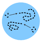
(a) Polymerization

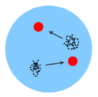
(b) Nucleation

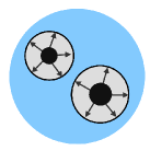
(c) Growth

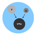
(d) Aggregation

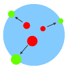
(e) Migration

Figure 1: Reaction mechanisms driving morphology development in a single polymer particle [ $\bullet$]: 1(a) polymerization of Monomer 2 [ ] into Polymer 2 chains [     ], 1(b) nucleation of Polymer 2 agglomerates [     ] into non-equilibrium clusters [ $\bullet$], 1(c) growth of equilibrium and non-equilibrium clusters in volumes, 1(d) aggregation of equilibrium and non-equilibrium clusters with sizes $v$ and $u$ into a cluster of a size $v+u$, 1(e) migration of non-equilibrium clusters [ $\bullet$] to equilibrium positions [ $\bullet$].

For the reaction mechanisms discussed above, we have introduced in [9] the dimensionless Population Balance Model (PBM) for Latex Particles Morphology Formation (LPMF). From now on we shall call it LPMF PBMReducing model complexity by means of the Optimal Scaling: Population Balance Model for latex particles morphology formation. The model predicts the evolution of the size distributions $m(v,t)$ and $w(v,t)$ of non-equilibrium and equilibrium polymer clusters composing the morphology of interest. The distributions $m(v,t)$ and $w(v,t)$ satisfy the system (1)-(13) of Population Balance Equations (PBE), which accounts for the polymerization, nucleation, growth, aggregation and migration processes.

$$\begin{cases}\frac{\partial m(v,t)}{\partial t}&=-\underbrace{\frac{\partial(\,g(v,t)\,m(v,t)\,)}{\partial v}}_{\text{Growth}}\,+\,\underbrace{n(v,t)}_{\text{Nucleation}}\,-\,\underbrace{\mu\,m(v,t)}_{\text{Migration}}-\,\underbrace{m(v,t)\,\int_{0}^{\infty}\!\alpha(v,u,t)\,m(u,t)\,du}_{\text{Aggregation}}\\ &\quad+\underbrace{\frac{1}{2}\,\int_{0}^{v}\!\alpha(v-u,u,t)\,m(v-u,t)\,m(u,t)\,du}_{\text{Aggregation}},\quad\quad\quad\forall v,t\in\mathbb{R}^{+},\\ \\ \frac{\partial w(v,t)}{\partial t}&=-\underbrace{\frac{\partial(\,g(v,t)\,w(v,t)\,)}{\partial v}}_{\text{Growth}}\,+\,\underbrace{\mu\,m(v,t)}_{\text{Migration}}-\,\underbrace{w(v,t)\,\int_{0}^{\infty}\!\alpha(v,u,t)\,w(u,t)\,du}_{\text{Aggregation}}\\ &\quad+\underbrace{\frac{1}{2}\,\int_{0}^{v}\!\alpha(v-u,u,t)\,w(v-u,t)\,w(u,t)\,du}_{\text{Aggregation}},\quad\quad\quad\forall v,t\in\mathbb{R}^{+},\\ \\ m(v,0)&=w(v,0)=0,\quad\forall v\in\mathbb{R}^{+},\quad\quad\quad m(0,t)=w(0,t)=0,\quad\forall t\in\mathbb{R}^{+},\end{cases}$$ (1)

$$\alpha(v,u,t):=\,\tilde{\alpha}_{0}(t)\,\left[v^{a}+u^{a}\right],\quad\tilde{\alpha}_{0}(t):=\,\lambda_{\mathrm{a}}\,(\Psi(t)+1)^{\nicefrac{{14}}{{3}}},$$ (2)

$$g(v,t):=\,\tilde{\varrho}_{\mathrm{d}}(t)\,v^{b}+\,\tilde{\varrho}_{\mathrm{p}}(t)\,v,\quad\tilde{\varrho}_{\mathrm{p}}(t):=\,\lambda_{\mathrm{p}}\,\frac{\Psi(t)}{V_{p}(t)},\quad\tilde{\varrho}_{\mathrm{d}}(t):=\,\lambda_{\mathrm{d}}\,\Phi(t)\,(\Psi(t)+1)^{\nicefrac{{2}}{{3}}},$$ (3)

$$n(v,t):=\,\tilde{\eta}_{0}(t)\,\delta(v-v_{0}),\quad\tilde{\eta}_{0}(t):=\,\lambda_{\mathrm{n}}\,\Phi(t),\quad v_{0}:=\lambda_{\mathrm{c}},\quad\mbox{with }\delta(x)\mbox{ the Dirac delta},$$ (4)

$$\mu:=\lambda_{\mathrm{m}},$$ (5)

$$\begin{cases}\frac{dV^{\mathrm{mat}}_{\mathrm{pol2}}(t)}{dt}&=\,\lambda_{\mathrm{p}}\,\frac{\Psi(t)}{V_{p}(t)}\,\left[\,V^{\mathrm{mat}}_{\mathrm{pol2}}(t)\,+\,\lambda_{\mathrm{pol1}}\,\right]-\,\Phi(t)\,\left[\,\lambda_{\mathrm{c}}\,\lambda_{\mathrm{n}}+\,\lambda_{\mathrm{d}}\,\Sigma_{m}(t)+\,\lambda_{\mathrm{d}}\,\Sigma_{w}(t)\right],\\ V^{\mathrm{mat}}_{\mathrm{pol2}}(0)&=\,0,\end{cases}$$ (6)

$$\begin{cases}\frac{dV^{\mathrm{c_{m}}}_{\mathrm{pol2}}(t)}{dt}&=\,\lambda_{\mathrm{p}}\,\frac{\Psi(t)}{V_{p}(t)}\,V^{\mathrm{c_{m}}}_{\mathrm{pol2}}(t)+\,\Phi(t)\,\left[\,\lambda_{\mathrm{c}}\,\lambda_{\mathrm{n}}+\,\lambda_{\mathrm{d}}\,\Sigma_{m}(t)\,\right]-\,\lambda_{\mathrm{m}}\,V^{\mathrm{c_{m}}}_{\mathrm{pol2}}(t),\\ V^{\mathrm{c_{m}}}_{\mathrm{pol2}}(0)&=\,0,\end{cases}$$ (7)

$$\begin{cases}\frac{dV^{\mathrm{c_{w}}}_{\mathrm{pol2}}(t)}{dt}&=\,\lambda_{\mathrm{p}}\,\frac{\Psi(t)}{V_{p}(t)}\,V^{\mathrm{c_{w}}}_{\mathrm{pol2}}(t)+\,\lambda_{\mathrm{d}}\,\Phi(t)\,\Sigma_{w}(t)+\,\lambda_{\mathrm{m}}\,V^{\mathrm{c_{m}}}_{\mathrm{pol2}}(t),\\ V^{\mathrm{c_{w}}}_{\mathrm{pol2}}(0)&=\,0,\end{cases}$$ (8)

$$\begin{cases}\frac{d\Psi(t)}{dt}&=-\lambda_{\mathrm{p}}\,\frac{\Psi(t)}{\Psi(t)+1}\,\frac{\Psi(t)+\Psi_{r}}{V_{\mathrm{pol2}}(t)+\lambda_{\mathrm{pol1}}},\\ \Psi(0)&=\,\bar{\Psi},\end{cases}$$ (9)

$$\begin{cases}\frac{dV_{\mathrm{pol2}}(t)}{dt}&=\,\lambda_{\mathrm{p}}\,\frac{\Psi(t)}{\Psi(t)+1},\\ V_{\mathrm{pol2}}(0)&=\,0,\end{cases}$$ (10)

$$\Phi(t):=\max\left\{\frac{V^{\mathrm{mat}}_{\mathrm{pol2}}(t)}{(\Psi(t)+1)(V^{\mathrm{mat}}_{\mathrm{pol2}}(t)+\lambda_{\mathrm{pol1}})}-\Phi_{s},0\right\},$$ (11)

$$V_{p}(t):=\,\left(\Psi(t)+1\right)\,\left[\,V^{\mathrm{mat}}_{\mathrm{pol2}}(t)+V^{\mathrm{c_{m}}}_{\mathrm{pol2}}(t)+V^{\mathrm{c_{w}}}_{\mathrm{pol2}}(t)+\lambda_{\mathrm{pol1}}\,\right],$$ (12)

$$\Sigma_{y}(t):=\,(\Psi(t)+1)^{\nicefrac{{2}}{{3}}}\int_{0}^{\infty}\!v^{b}\,y(v,t)\,dv,\quad y=m,w.$$ (13)

The coefficients appearing in (1)-(13) are defined in Table 1 and Table 2, while Appendix F provides a glossary for the variables in (1)-(13) and governing parameters in Tables 1-2. We remark that the factors $\theta$ and the experimental parameters $\tilde{p}$ in Tables 1-2 are dimensional quantities as they possess units of measure, e.g., $\nu_{0}$ is expressed in Litres, $t_{0}$ in seconds and $d_{0}$ in Litres^-1. Since the chosen system of units is consistent, for simplicity, in the following sections we discard the units of measure of all the dimensional quantities and treat any dimensional variable $X$ as $X/c_{X}$, with $c_{X}=1$ to be the unit of $X$.

Given $\tilde{p}=\tilde{p}_{\mathrm{exp}}$ (see Table 2), a particular choice of scaling factors $\theta:=\{\nu_{0},t_{0},d_{0}\}$ in Table 1 fully defines a scaling regime of the proposed model and provides values of corresponding coefficients $\lambda(\theta,\tilde{p})$. For example, by setting $\theta=\{1,\dots,1\}$ one can restore the coefficients $\lambda$ of the unscaled LPMF PBMReducing model complexity by means of the Optimal Scaling: Population Balance Model for latex particles morphology formation. Different scaling regimes of the PBM (1)-(13) were proposed and compared in [9]. The Optimal Scaling (OSReducing model complexity by means of the Optimal Scaling: Population Balance Model for latex particles morphology formation) was found to be best in terms of its ability to produce scaled coefficients of similar orders of magnitude. This prevented severe round-off errors, improved conditioning of the considered problem and hindered unphysical behaviour of the computed solution. In the following sections we explore yet another scaling regime for LPMF PBMReducing model complexity by means of the Optimal Scaling: Population Balance Model for latex particles morphology formation.

Coefficients $\lambda$	$\lambda(\theta,\tilde{p})$
$\lambda_{\mathrm{a}}$	$\lambda_{\mathrm{a}}=\kappa_{1}\,\nu_{0}^{a+1}\,t_{0}\,d_{0}$,	$\kappa_{1}=k_{\mathrm{a}}/N_{\mathrm{p}}$
$\lambda_{\mathrm{c}}$	$\lambda_{\mathrm{c}}=\kappa_{2}\,\nu_{0}^{-1}$,	$\kappa_{2}=v_{\mathrm{c}}$
$\lambda_{\mathrm{d}}$	$\lambda_{\mathrm{d}}=\kappa_{3}\,\nu_{0}^{b-1}\,t_{0}$,	$\kappa_{3}=\sqrt[3]{36\pi}\,k_{\mathrm{d}}$
$\lambda_{\mathrm{m}}$	$\lambda_{\mathrm{m}}=\kappa_{4}\,t_{0}$,	$\kappa_{4}=k_{\mathrm{m}}$
$\lambda_{\mathrm{n}}$	$\lambda_{\mathrm{n}}=\kappa_{5}\,\nu_{0}^{-1}\,t_{0}\,d_{0}^{-1}$,	$\kappa_{5}=k_{\mathrm{n}}/v_{\mathrm{c}}$
$\lambda_{\mathrm{p}}$	$\lambda_{\mathrm{p}}=\kappa_{6}\,\nu_{0}^{-2}\,t_{0}\,d_{0}^{-1}$,	$\kappa_{6}=k_{\mathrm{p}}\,R\,\bar{V}_{\mathrm{pol2}}/\bar{V}_{\mathrm{mon2}}$
$\lambda_{\mathrm{pol1}}$	$\lambda_{\mathrm{pol1}}=\kappa_{7}\,\nu_{0}^{-2}\,d_{0}^{-1}$,	$\kappa_{7}=V_{\mathrm{pol1}}$
Other Coefficients	Numerical Values
$a$	$-1/3$
$b$	$2/3$
$\bar{\Psi}$	$1$
$\Psi_{r}$	$20/19$
$\Phi_{s}$	$10^{-3}$

Table 1: Dimensionless coefficients $\lambda(\theta,\tilde{p})\in(0,\infty)^{7}$, $a$, $b$, $\bar{\Psi}$, $\Psi_{r}$, $\Phi_{s}$, with dimensional scaling factors $\theta:=\{\nu_{0},t_{0},d_{0}\}$ and physical parameters $\tilde{p}:=\{k_{\mathrm{a}},k_{\mathrm{d}},k_{\mathrm{p}},k_{\mathrm{n}},k_{\mathrm{m}},v_{\mathrm{c}},N_{\mathrm{p}},R,V_{\mathrm{pol1}},\bar{V}_{\mathrm{mon2}},\bar{V}_{\mathrm{pol2}}\}$ (Table 2) of the equations (1)-(13) derived in [9]. The defined here coefficients $\lambda$ arise by setting the scaling factors $\{\nu_{0},t_{0},m_{0},w_{0},M_{0},P_{0},\Pi_{0},\delta_{0}\}$ proposed in [9] as $m_{0}=w_{0}=d_{0}$, $M_{0}=P_{0}=\Pi_{0}=d_{0}\,\nu_{0}^{2}$ and $\delta_{0}=1/\nu_{0}$. The numerical values of $a$, $b$, $\bar{\Psi}$, $\Psi_{r}$ and $\Phi_{s}$ correspond to the physically grounded model [7, 9], while the models and derivations presented in what follows are valid for any finite value of $a\leq 0$, $b\in(0,1)$, $\bar{\Psi}>0$, $\Psi_{r}>0$ and $\Phi_{s}\in(0,1)$.

Parameters $\tilde{p}$	Values $\tilde{p}_{\mathrm{exp}}$
$k_{\mathrm{a}}$	see Section 5
$k_{\mathrm{d}}$	$10^{-17}\,\mathrm{L}^{1-b}\,\mathrm{s}^{-1}$
$k_{\mathrm{p}}$	$850\,\mathrm{L}\,\mathrm{mol}^{-1}\,\mathrm{s}^{-1}$
$k_{\mathrm{n}}$	$2.5\times 10^{-5}\,\mathrm{L}\,\mathrm{s}^{-1}$
$k_{\mathrm{m}}$	$10^{-5}\,\mathrm{s}^{-1}$
$v_{\mathrm{c}}$	$2.5\times 10^{-22}\,\mathrm{L}$

Parameters $\tilde{p}$	Values $\tilde{p}_{\mathrm{exp}}$
$N_{\mathrm{p}}$	$2.8\times 10^{17}$
$R$	$2.3\times 10^{-7}\,\mathrm{mol}$
$V_{\mathrm{pol1}}$	$0.25\,\mathrm{L}$
$\bar{V}_{\mathrm{mon2}}$	$0.1\,\mathrm{L}\,\mathrm{mol}^{-1}$
$\bar{V}_{\mathrm{pol2}}$	$0.095\,\mathrm{L}\,\mathrm{mol}^{-1}$

Table 2: Experimental values of parameters $\tilde{p}:=\{k_{\mathrm{a}},k_{\mathrm{d}},k_{\mathrm{p}},k_{\mathrm{n}},k_{\mathrm{m}},v_{\mathrm{c}},N_{\mathrm{p}},R,V_{\mathrm{pol1}},\bar{V}_{\mathrm{mon2}},\bar{V}_{\mathrm{pol2}}\}$ involved in the computation of the dimensionless coefficients in Table 1 as proposed in [7]. The symbols $\mathrm{s}$, $\mathrm{L}$ and $\mathrm{mol}$ stand for second, Litre and mole respectively. Some alternative values of $k_{\mathrm{d}}$, $k_{\mathrm{n}}$ and $v_{\mathrm{c}}$ are also considered in Section 5.

3 Reducing Complexity of the LPMF PBM Using Optimal Scaling

Here we revisit the OSReducing model complexity by means of the Optimal Scaling: Population Balance Model for latex particles morphology formation scaling of the model (1)-(13) and propose to apply OSReducing model complexity by means of the Optimal Scaling: Population Balance Model for latex particles morphology formation along with the specific constraints on $\lambda$ coefficients (Table 1) with the purpose to reduce the complexity of (1)-(13). More precisely, we wish to introduce a particular regime of coefficients

$$\lambda(\theta,\tilde{p}):=\{ \lambda_{\mathrm{a}}=\lambda_{1}(\theta,\tilde{p}),\lambda_{\mathrm{c}}=\lambda_{2}(\theta,\tilde{p}),\lambda_{\mathrm{d}}=\lambda_{3}(\theta,\tilde{p}),$$

$$\lambda_{\mathrm{m}}=\lambda_{4}(\theta,\tilde{p}),\lambda_{\mathrm{n}}=\lambda_{5}(\theta,\tilde{p}),\lambda_{\mathrm{p}}=\lambda_{6}(\theta,\tilde{p}),$$

$$\lambda_{\mathrm{pol1}}=\lambda_{7}(\theta,\tilde{p})\}\in(0,\infty)^{N_{d}},\quad N_{d}=7,$$ (14)

leading to negligible weights of the integral terms in (1).

To achieve these goals, first, it is necessary to prove that the condition $\lambda_{\mathrm{a}}\to 0$ (see (1)-(2)) implies diminishing the integral terms. Then the scaling procedure supporting such a condition on $\lambda_{\mathrm{a}}$ and maintaining similar orders of magnitude for other scaled coefficients has to be established.

3.1 Discarding Integral Terms in the LPMF PBM

We consider the following regime for coefficients $\lambda(\theta,\tilde{p})$ (14):

$$\lambda_{\mathrm{a}}\ll 1\quad\mbox{and the deviation of}\quad\{\lambda_{\mathrm{c}},\lambda_{\mathrm{d}},\lambda_{\mathrm{m}},\lambda_{\mathrm{n}},\lambda_{\mathrm{p}},\lambda_{\mathrm{pol1}}\}\quad\mbox{from}\quad\{1,1,1,1,1,1\}$$ (15)

$$\mbox{is minimal, regardless of the values of}\quad\lambda_{\mathrm{a}}.$$

Next we demonstrate that given $a\leq 0$, $0<b<1$ and $v_{0}>0$, the integral terms in (1) tend to $0$ when $\lambda_{\mathrm{a}}\to 0$ and $\lambda_{\mathrm{c}},\lambda_{\mathrm{d}},\lambda_{\mathrm{m}},\lambda_{\mathrm{n}},\lambda_{\mathrm{p}},\lambda_{\mathrm{pol1}}$ are constants with magnitudes $\approx 10^{0}$, as specified in (15). In this section, we briefly explain the ideas behind the formal proof, leaving the detailed arguments for Appendices A-E.

In order to investigate the limit for $\lambda_{\mathrm{a}}\to 0$ of solutions to (1)-(13), we multiply $\lambda_{\mathrm{a}}$ in (1)-(2) by $\epsilon>0$ and consider the limit for $\epsilon\to 0$ of solutions to the arising equation with the constant $\lambda_{\mathrm{a}},\lambda_{\mathrm{c}},\lambda_{\mathrm{d}},\lambda_{\mathrm{m}},\lambda_{\mathrm{n}},\lambda_{\mathrm{p}},\lambda_{\mathrm{pol1}}$:

$$\frac{\partial m_{\epsilon}(v,t)}{\partial t} =-\frac{\partial(\,g(v,t)\,m_{\epsilon}(v,t)\,)}{\partial v}\,+\,n(v,t)\,-\,\mu\,m_{\epsilon}(v,t)-\,m_{\epsilon}(v,t)\,\int_{0}^{\infty}\!\epsilon\,\alpha(v,u,t)\,m_{\epsilon}(u,t)\,du\,+$$

$$\quad+\frac{1}{2}\,\int_{0}^{v}\!\epsilon\,\alpha(v-u,u,t)\,m_{\epsilon}(v-u,t)\,m_{\epsilon}(u,t)\,du,\quad\quad\quad\forall v,t\in\mathbb{R}^{+}.$$ (16)

It can be shown that $m_{\epsilon}$ is bounded in a suitable manner, independent of $\epsilon$. Thus, one expects that as $\epsilon\to 0$ the integral terms in the above equation will have a vanishing influence. Moreover, it is natural to presume that the corresponding solutions $m_{\epsilon}$ tend to the limit $m_{0}$, that is also a solution of the equation formally obtained by setting $\epsilon=0$. Given that $m_{\epsilon}$ is bounded uniformly in $\epsilon$, the danger in this setting are the possible increasing oscillations as $\epsilon\to 0$. These can be controlled using the equation, namely the fact that the time oscillations, i.e. the time derivative of $m_{\epsilon}$, is also controlled (using the terms on the right hand side). The existing bounds on $m_{\epsilon}$ allow a very weak control on the terms on the right hand side and thus the convergence will take place in a suitably weak sense, namely

$$\sup_{t\in[0,T]}\int_{0}^{V}\!(m_{\epsilon_{k}}(v,t)-m_{0}(v,t))\,\varphi(v,t)\,dv\to 0,\textrm{ as }k\to\infty,$$ (17)

for some sequence $(\epsilon_{k})_{k\in\mathbb{N}}$ with $\epsilon_{k}\to 0$ as $k\to\infty$ and for any function $\varphi:(0,V)\times[0,T]\to\mathbb{R}$ which is at least differentiable in both variables and for each $t\in[0,T]$ is zero on intervals of type $(0,\delta_{t})\cup(V-\delta_{t},V)$. A similar argument can be applied to the corresponding $w_{\epsilon}$ equations, but we shall omit it. The details and proof of this convergence are presented in Appendix E, whereas the essential conditions for such convergence, namely the boundedness of PBE solutions and the finiteness of PBE solutions’ moments are proved in Appendix D and Appendix C respectively.

3.2 Optimal Scaling with Constraints (OSC)

We first summarise the Optimal Scaling (OS) procedure developed in [9] and then show how to modify the OSReducing model complexity by means of the Optimal Scaling: Population Balance Model for latex particles morphology formation methodology in order to achieve the regime (15).

The coefficients $\lambda(\theta,\tilde{p})$ (14) depend on the scaling factors $\theta:=\{\theta_{j}\}_{j=1}^{N_{x}}\in(0,\infty)^{N_{x}}$, where

$$\theta=\{\nu_{0},t_{0},d_{0}\}\in(0,\infty)^{N_{x}},\quad N_{x}=3,$$ (18)

and physical parameters

$$\tilde{p}=\{k_{\mathrm{a}},k_{\mathrm{d}},k_{\mathrm{p}},k_{\mathrm{n}},k_{\mathrm{m}},v_{\mathrm{c}},N_{\mathrm{p}},R,V_{\mathrm{pol1}},\bar{V}_{\mathrm{mon2}},\bar{V}_{\mathrm{pol2}}\}\in(0,\infty)^{\tilde{N}},\quad\tilde{N}=11.$$ (19)

The explicit formulas for $\lambda=\lambda(\theta,\tilde{p})$ and the experimental values $\tilde{p}_{\mathrm{exp}}$ of parameters $\tilde{p}$ are provided in Table 1 and Table 2. We notice that the units of measure of $\theta$ and $\tilde{p}$ are discarded as explained in Section 2.

As in most physical situations, the coefficients $\lambda$ (see for instance the case in (14), i.e. Table 1) can be presented in terms of governing parameters [11] as

$$\lambda_{i}(\theta,\tilde{p})=\kappa_{i}\,\theta^{\alpha^{i}_{1}}_{1}\dots\theta^{\alpha^{i}_{N_{x}}}_{N_{x}},\quad\kappa_{i}=\kappa_{i}(\tilde{p}):(0,\infty)^{\tilde{N}}\to(0,\infty),\quad\alpha^{i}_{j}\in\mathbb{R},$$ (20)

for all $i=1,\dots,N_{d}$ and $j=1,\dots,N_{x}$. Given $\tilde{p}$, $\{\alpha^{i}_{j}\}_{i,j=1}^{N_{d},N_{x}}$ and $\Theta:=\{\Theta_{i}\}_{i=1}^{N_{d}}\in\mathbb{R}^{N_{d}}$, the OSReducing model complexity by means of the Optimal Scaling: Population Balance Model for latex particles morphology formation procedure designed in [9] identifies the factors $\theta$ leading to the minimal distance between the orders of magnitude of coefficients $\lambda$ and the vector $\Theta$. In particular, such factors $\theta$ are obtained as the optimum $\theta_{\mathrm{opt}}$ of the cost function $C(\theta):(0,\infty)^{N_{x}}\to[0,\infty)$, i.e.

$$\theta_{\mathrm{opt}}:=\mathop{\mathrm{argmin}}_{\theta\in(0,\infty)^{N_{x}}}C(\theta),\quad C(\theta):=\sum_{i=1}^{N_{d}}\left[\log_{10}(\lambda_{i}(\theta,\tilde{p}))-\Theta_{i}\right]^{2},$$ (21)

with $\lambda_{i}$ being the $i$-th component of vector $\lambda$ (14) and $\Theta_{i}$ chosen as the desired order of magnitude of $\lambda_{i}$, $\forall i=1,\dots,N_{d}$.

As demonstrated in [9], the problem (21) can be solved as

$$\left(\sum_{i=1}^{N_{d}}\alpha^{i}_{1}\alpha^{i}_{j}\right)\,\rho^{\star}_{1}\,+\,\dots\,+\,\left(\sum_{i=1}^{N_{d}}\alpha^{i}_{N_{x}}\alpha^{i}_{j}\right)\,\rho^{\star}_{N_{x}}=\log_{10}(\hat{\kappa}_{j}),\quad\forall j=1,\dots,N_{x},$$ (22)

where $\rho^{\star}_{1},\dots,\rho^{\star}_{N_{x}}$ are defined as $\theta_{\mathrm{opt}}=\left\{10^{\rho^{\star}_{j}}\right\}_{j=1}^{N_{x}}$ and $\hat{\kappa}_{j}:=\prod_{i=1}^{N_{d}}\kappa_{i}^{-\alpha^{i}_{j}}\,10^{\sum_{i=1}^{N_{d}}\alpha^{i}_{j}\Theta_{i}}$, $\forall j=1,\dots,N_{x}$.

In order to achieve the regime (15) of coefficients $\lambda$ proposed in Section 3.1, the just described OSReducing model complexity by means of the Optimal Scaling: Population Balance Model for latex particles morphology formation procedure is modified as follows. Given $\tilde{p}$, $\{\alpha^{i}_{j}\}_{i,j=1}^{N_{d},N_{x}}$ and $\Theta_{2},\dots,\Theta_{N_{d}}$, we consider the metric $C$ (21) to be a function of the augmented argument $\tilde{\theta}$:

$$\tilde{\theta}:=\{\theta,\Theta_{1}\}\in(0,\infty)^{N_{x}}\times\mathbb{R},\quad\theta:=\{\theta_{1},\dots,\theta_{N_{x}}\}\in(0,\infty)^{N_{x}}.$$ (23)

Then, the values of $\tilde{\theta}$ are selected by minimising the distance $C(\tilde{\theta})$ between the magnitudes of coefficients $\lambda$ and the vector $\Theta$, subjected to the following constraint:

$$\tilde{\theta}_{\mathrm{opt}}:=\mathop{\mathrm{argmin}}_{\tilde{\theta}=\{\theta,\Theta_{1}\}}C(\tilde{\theta}),\quad\Theta_{1}\leq q_{1},$$ (24)

with $q_{1}\in\mathbb{R}$ a predefined parameter.

In what follows, we explain how to find a solution to (24) and, thus, to determine the factors

$$\tilde{\theta}^{N_{x}}_{\mathrm{opt}}:=\{\theta^{\star}_{1},\dots,\theta^{\star}_{N_{x}}\}\in(0,\infty)^{N_{x}}$$ (25)

corresponding to $\tilde{\theta}_{\mathrm{opt}}=\{\theta^{\star}_{1},\dots,\theta^{\star}_{N_{x}},\Theta^{\star}_{1}\}$ (24).

The functional shape (20) of the coefficients $\lambda$ and the change of variables $\rho_{j}:=\log_{10}(\theta_{j})$, $\forall j=1,\dots,N_{x}$, allow us to write the function $C$ (21) of the augmented argument $\tilde{\theta}$ (23) as

$$C(\tilde{\rho})=\sum_{i=1}^{N_{d}}\left[\log_{10}(\kappa_{i})+\sum_{j=1}^{N_{x}}\alpha^{i}_{j}\rho_{j}-\Theta_{i}\right]^{2},\quad\forall\tilde{\rho}:=\{\rho_{1},\dots,\rho_{N_{x}},\Theta_{1}\}\in\mathbb{R}^{N_{x}+1},$$ (26)

with $\kappa_{i}>0$ and $\alpha^{i}_{j},\Theta_{2},\dots,\Theta_{N_{d}}\in\mathbb{R}$ being fixed parameters $\forall i,j=1,\dots,N_{d,x}$. Then, (24) reads as

$$\begin{cases}\tilde{\rho}_{\mathrm{opt}}&:=\mathop{\mathrm{argmin}}_{\tilde{\rho}\in\Omega}C(\tilde{\rho}),\\ \Omega&:=\{\tilde{\rho}\in\mathbb{R}^{N_{x}+1}\,|\,g_{1}(\tilde{\rho})\geq 0\},\\ g_{1}(\tilde{\rho})&:=-\Theta_{1}+q_{1},\end{cases}$$ (27)

where $C(\tilde{\rho})$ and $\tilde{\rho}$ are given in (26), $g_{1}:\mathbb{R}^{N_{x}+1}\to\mathbb{R}$ and $q_{1}\in\mathbb{R}$ is a predefined parameter. Since the equation $c\,\nabla g_{1}=0$ admits the only solution $c=0$ (where $c$ is a scalar), i.e. the linear independence constraint qualification (LICQ) holds at any $\tilde{\rho}\in\mathbb{R}^{N_{x}+1}$, there exists $l_{1}\in\mathbb{R}$ such that the following Karush-Kuhn-Tucker conditions (see [12] Chapter 12) are satisfied by any local minimum of $C$ in $\Omega$ (27):

$$\begin{cases}&\nabla_{\tilde{\rho}}\mathcal{L}(\tilde{\rho},l_{1})=0,\\ &l_{1}\,g_{1}(\tilde{\rho})=0,\\ &g_{1}(\tilde{\rho}),\,l_{1}\geq 0.\end{cases}$$ (28)

Here the Lagrangian function $\mathcal{L}:\mathbb{R}^{N_{x}+2}\to\mathbb{R}$ is defined as

$$\mathcal{L}(\tilde{\rho},l_{1}):=C(\tilde{\rho})-l_{1}\,g_{1}(\tilde{\rho}),\quad\forall\tilde{\rho}\in\mathbb{R}^{N_{x}+1},\quad\forall l_{1}\in\mathbb{R},$$ (29)

with $l_{1}$ known as Lagrange multiplier [13].

Denoting $x_{1}:=g_{1}(\tilde{\rho})$, one gets from (28) the following system of $N_{x}+3$ equations with $N_{x}+3$ unknowns $\{\rho_{1},\dots,\rho_{N_{x}},\Theta_{1},x_{1},l_{1}\}\in\mathbb{R}^{N_{x}+3}$:

$$\left\{\begin{aligned} \Theta_{1}+x_{1}&=q_{1},\\ \sum_{k=1}^{N_{x}}\left(\sum_{i=1}^{N_{d}}\alpha^{i}_{j}\,\alpha^{i}_{k}\right)\rho_{k}-\alpha^{1}_{j}\,\Theta_{1}&=\sum_{i=2}^{N_{d}}\alpha^{i}_{j}\,\Theta_{i}-\sum_{i=1}^{N_{d}}\alpha^{i}_{j}\,\log_{10}(\kappa_{i}),\quad j=1,\dots,N_{x},\\ \sum_{k=1}^{N_{x}}\alpha^{1}_{k}\,\rho_{k}-\Theta_{1}-l_{1}/2&=-\log_{10}(\kappa_{1}),\\ l_{1}\,x_{1}&=0,\end{aligned}\right.$$ (30)

whose only admissible solutions are those corresponding to $x_{1},l_{1}\geq 0$.

Equations (30) along with the predefined $q_{1}$, $\Theta_{2},\dots,\Theta_{N_{d}}\in\mathbb{R}$, $\alpha^{i}_{j}\in\mathbb{R}$ and $\kappa_{i}>0$, $\forall i,j=1,\dots,N_{d,x}$, give rise to two linear systems if $l_{1}\,x_{1}=0$ is replaced with one of the two possible solutions

$$l_{1}=0,$$ (31)

$$x_{1}=0.$$ (32)

From now on we shall refer to the system (30)-(31) as $(S_{1})$ and to the system comprising (30), (32) as $(S_{2})$.

Then $\tilde{\rho}_{\mathrm{opt}}=\{\rho^{\star}_{1},\dots,\rho^{\star}_{N_{x}},\Theta^{\star}_{1}\}$ can be calculated as solution to either $(S_{1})$ or $(S_{2})$ in such a way that $(i)$ a system admits a solution, $(ii)$ $x_{1},l_{1}\geq 0$ and $(iii)$ the cost $C$ (26) is minimal. Finally, we compute $\tilde{\theta}_{\mathrm{opt}}$ (24) and the factors $\tilde{\theta}^{N_{x}}_{\mathrm{opt}}$ (25) as

$$\tilde{\theta}_{\mathrm{opt}}=\{10^{\rho^{\star}_{1}},\dots,10^{\rho^{\star}_{N_{x}}},\Theta^{\star}_{1}\},\quad\tilde{\theta}^{N_{x}}_{\mathrm{opt}}=\{10^{\rho^{\star}_{1}},\dots,10^{\rho^{\star}_{N_{x}}}\}.$$ (33)

The computed $\tilde{\rho}_{\mathrm{opt}}$ is a global solution of the constrained minimisation problem (27), because $C(\tilde{\rho})$ and $-g_{1}(\tilde{\rho})$ are convex functions of $\tilde{\rho}\in\mathbb{R}^{N_{x}+1}$, as shown in [14, 15]. In particular, the Hessian $\nabla_{\tilde{\rho}}\nabla_{\tilde{\rho}}\,C$ is a positive semi-definite matrix $\forall\tilde{\rho}\in\mathbb{R}^{N_{x}+1}$ and $-g_{1}(\tilde{\rho})$ is an affine, thus, convex function of $\tilde{\rho}\in\mathbb{R}^{N_{x}+1}$. Then, $\tilde{\theta}_{\mathrm{opt}}$ (33) provides a global optimum for the problem (24).

To sum up, we adapted the OSReducing model complexity by means of the Optimal Scaling: Population Balance Model for latex particles morphology formation methodology to the problems with a constrained parameter, such as the scaling regime (15), and reformulated the OSReducing model complexity by means of the Optimal Scaling: Population Balance Model for latex particles morphology formation minimisation problem (21) as (24). The optimal factors (25) are then computed by solving a linear system selected between $(S_{1})$ and $(S_{2})$. We remark that the same formulation can be used if in (24) a constraint is applied to any of the coefficients $\lambda$ (14). Moreover, it should be possible to derive linear systems of the form $(S_{1})$ or $(S_{2})$ in a similar manner, when required constraints differ from (24).

In what follows we shall refer to the new scaling procedure as Optimal Scaling with Constraints or OSCReducing model complexity by means of the Optimal Scaling: Population Balance Model for latex particles morphology formation.

3.3 Computation of Dimensionless Coefficients of the LPMF PBM using OSC

With the aim of achieving the regime (15) in the LPMF PBMReducing model complexity by means of the Optimal Scaling: Population Balance Model for latex particles morphology formation (1)-(13), we apply the OSCReducing model complexity by means of the Optimal Scaling: Population Balance Model for latex particles morphology formation procedure proposed in Section 3.2 to the coefficients $\lambda$ (14) defined in Table 1. We remark that the results provided in this section correspond to the physically grounded values of $a=-1/3$ and $b=2/3$, as specified in Table 1.

Hence, we consider $N_{d}=7$ dimensionless coefficients $\lambda$ and $N_{x}=3$ scaling factors $\theta=\{\nu_{0},t_{0},d_{0}\}$ (see Table 1). Let us denote $\rho_{1}:=\log_{10}(\nu_{0})$, $\rho_{2}:=\log_{10}(t_{0})$, $\rho_{3}:=\log_{10}(d_{0})$ and assign $\Theta_{2}=\Theta_{3}=\dots=\Theta_{7}=0$ in order to satisfy the second condition in (15). Then, $(S_{1})$ and $(S_{2})$, each admitting a unique solution $\forall q_{1}\in\mathbb{R}$, read as:

$$(S_{1}):\begin{cases}\nu_{0}&=\frac{\kappa_{2}^{9/16}\left(\kappa_{3}\,\kappa_{6}\,\kappa_{7}\right)^{3/16}}{\kappa_{5}^{3/8}},\\ t_{0}&=\frac{\kappa_{7}^{1/4}}{\left(\kappa_{3}^{3}\,\kappa_{4}^{3}\,\kappa_{5}\,\kappa_{6}\right)^{1/8}},\\ d_{0}&=\frac{\kappa_{5}^{7/8}\,\kappa_{7}^{3/16}}{\kappa_{4}^{1/4}\left(\kappa_{2}^{15}\,\kappa_{3}^{9}\,\kappa_{6}\right)^{1/16}},\\ \Theta_{1}&=\log_{10}\left(\kappa_{1}\sqrt[16]{\frac{\kappa_{5}^{8}\,\kappa_{7}^{9}}{\kappa_{2}^{9}\,\kappa_{3}^{13}\,\kappa_{4}^{10}\,\kappa_{6}}}\right),\\ x_{1}&=q_{1}+\log_{10}\left(\frac{1}{\kappa_{1}}\sqrt[16]{\frac{\kappa_{2}^{9}\,\kappa_{3}^{13}\,\kappa_{4}^{10}\,\kappa_{6}}{\kappa_{5}^{8}\,\kappa_{7}^{9}}}\right),\\ l_{1}&=0,\end{cases}\quad(S_{2}):\begin{cases}\nu_{0}&=10^{-\frac{9q_{1}}{47}}\frac{\kappa_{1}^{9/47}\,\kappa_{2}^{171/376}\,\kappa_{3}^{3/94}\,\kappa_{6}^{33/188}\,\kappa_{7}^{111/376}}{\kappa_{4}^{45/376}\,\kappa_{5}^{105/376}},\\ t_{0}&=10^{\frac{10q_{1}}{47}}\frac{\kappa_{2}^{45/376}\,\kappa_{7}^{49/376}}{\kappa_{1}^{10/47}\,\kappa_{3}^{19/94}\,\kappa_{4}^{91/376}\,\kappa_{5}^{87/376}\,\kappa_{6}^{21/188}},\\ d_{0}&=10^{\frac{27q_{1}}{47}}\frac{\kappa_{4}^{41/376}\,\kappa_{5}^{221/376}}{\kappa_{1}^{27/47}\,\kappa_{2}^{231/376}\,\kappa_{3}^{9/94}\,\kappa_{6}^{5/188}\,\kappa_{7}^{51/376}},\\ \Theta_{1}&=q_{1},\\ x_{1}&=0,\\ l_{1}&=-\frac{2}{47}\left[16q_{1}+\log_{10}\left(\frac{\kappa_{2}^{9}\,\kappa_{3}^{13}\,\kappa_{4}^{10}\,\kappa_{6}}{\kappa_{1}^{16}\,\kappa_{5}^{8}\,\kappa_{7}^{9}}\right)\right],\end{cases}$$ (34)

with $\kappa_{1},\dots,\kappa_{7}$ provided in Table 1 and $x_{1},l_{1}\geq 0$ (see Section 3.2). We remark that the solutions of $(S_{1})$ and $(S_{2})$ in (34) are equivalent when $\pi_{0}=10^{q_{1}}$, where we denote

$$\pi_{0}:=\kappa_{1}\sqrt[16]{\frac{\kappa_{5}^{8}\,\kappa_{7}^{9}}{\kappa_{2}^{9}\,\kappa_{3}^{13}\,\kappa_{4}^{10}\,\kappa_{6}}}=\frac{(36\pi)^{-13/48}\,k_{\mathrm{a}}\,k_{\mathrm{n}}^{1/2}\,V_{\mathrm{pol1}}^{9/16}\,\bar{V}_{\mathrm{mon2}}^{1/16}}{N_{\mathrm{p}}\,v_{\mathrm{c}}^{17/16}\,k_{\mathrm{d}}^{13/16}\,k_{\mathrm{m}}^{5/8}\,\left(\,k_{\mathrm{p}}\,R\,\bar{V}_{\mathrm{pol2}}\,\right)^{1/16}},$$ (35)

with $\kappa_{1},\dots,\kappa_{7}$ from Table 1 and the other parameters given in Table 2. Since $x_{1}$ and $l_{1}$ must be always non-negative, the solution of $(S_{1})$ is admissible only if $\pi_{0}\leq 10^{q_{1}}$, whereas when $\pi_{0}>10^{q_{1}}$, the solution of $(S_{2})$ is permitted.

Then, for any given $q_{1}\in\mathbb{R}$, the optimal scaling factors $\tilde{\theta}^{N_{x}}_{\mathrm{opt}}=\{\nu_{0},t_{0},d_{0}\}$ correspond to $(S_{1})$ if $\pi_{0}\leq 10^{q_{1}}$, or $(S_{2})$ otherwise:

$$\begin{pmatrix}\nu_{0}\\ t_{0}\\ d_{0}\end{pmatrix}=\begin{cases}\begin{pmatrix}\frac{\kappa_{2}^{9/16}\left(\kappa_{3}\,\kappa_{6}\,\kappa_{7}\right)^{3/16}}{\kappa_{5}^{3/8}}\\ \frac{\kappa_{7}^{1/4}}{\left(\kappa_{3}^{3}\,\kappa_{4}^{3}\,\kappa_{5}\,\kappa_{6}\right)^{1/8}}\\ \frac{\kappa_{5}^{7/8}\,\kappa_{7}^{3/16}}{\kappa_{4}^{1/4}\left(\kappa_{2}^{15}\,\kappa_{3}^{9}\,\kappa_{6}\right)^{1/16}}\end{pmatrix}&\mbox{if}\quad\pi_{0}\leq 10^{q_{1}},\\ \\ \begin{pmatrix}10^{-\frac{9q_{1}}{47}}\frac{\kappa_{1}^{9/47}\,\kappa_{2}^{171/376}\,\kappa_{3}^{3/94}\,\kappa_{6}^{33/188}\,\kappa_{7}^{111/376}}{\kappa_{4}^{45/376}\,\kappa_{5}^{105/376}}\\ 10^{\frac{10q_{1}}{47}}\frac{\kappa_{2}^{45/376}\,\kappa_{7}^{49/376}}{\kappa_{1}^{10/47}\,\kappa_{3}^{19/94}\,\kappa_{4}^{91/376}\,\kappa_{5}^{87/376}\,\kappa_{6}^{21/188}}\\ 10^{\frac{27q_{1}}{47}}\frac{\kappa_{4}^{41/376}\,\kappa_{5}^{221/376}}{\kappa_{1}^{27/47}\,\kappa_{2}^{231/376}\,\kappa_{3}^{9/94}\,\kappa_{6}^{5/188}\,\kappa_{7}^{51/376}}\end{pmatrix}&\mbox{otherwise},\end{cases}$$ (36)

with $\kappa_{1},\dots,\kappa_{7}$ defined in Table 1 and $\pi_{0}$ in (35). As a result, the following are the coefficients $\lambda(\tilde{\theta}^{N_{x}}_{\mathrm{opt}},\tilde{p})$ (14) provided by OSCReducing model complexity by means of the Optimal Scaling: Population Balance Model for latex particles morphology formation (for any given $q_{1}\in\mathbb{R}$):

$$\begin{pmatrix}\lambda_{\mathrm{a}}\\ \lambda_{\mathrm{c}}\\ \lambda_{\mathrm{d}}\\ \lambda_{\mathrm{m}}\\ \lambda_{\mathrm{n}}\\ \lambda_{\mathrm{p}}\\ \lambda_{\mathrm{pol1}}\end{pmatrix}=\begin{pmatrix}\lambda_{1}(\tilde{\theta}^{N_{x}}_{\mathrm{opt}},\tilde{p})\\ \lambda_{2}(\tilde{\theta}^{N_{x}}_{\mathrm{opt}},\tilde{p})\\ \lambda_{3}(\tilde{\theta}^{N_{x}}_{\mathrm{opt}},\tilde{p})\\ \lambda_{4}(\tilde{\theta}^{N_{x}}_{\mathrm{opt}},\tilde{p})\\ \lambda_{5}(\tilde{\theta}^{N_{x}}_{\mathrm{opt}},\tilde{p})\\ \lambda_{6}(\tilde{\theta}^{N_{x}}_{\mathrm{opt}},\tilde{p})\\ \lambda_{7}(\tilde{\theta}^{N_{x}}_{\mathrm{opt}},\tilde{p})\end{pmatrix}=\begin{cases}\begin{pmatrix}\pi_{0}\\ \frac{\kappa_{2}^{7/16}\,\kappa_{5}^{3/8}}{\left(\kappa_{3}\,\kappa_{6}\,\kappa_{7}\right)^{3/16}}\\ \frac{\kappa_{3}^{9/16}\,\kappa_{7}^{3/16}}{\kappa_{2}^{3/16}\,\kappa_{4}^{3/8}\,\kappa_{6}^{3/16}}\\ \frac{\kappa_{4}\,\kappa_{7}^{1/4}}{\left(\kappa_{3}^{3}\,\kappa_{4}^{3}\,\kappa_{5}\,\kappa_{6}\right)^{1/8}}\\ \frac{\left(\kappa_{2}\,\kappa_{5}\right)^{3/8}}{\kappa_{6}^{1/4}\left(\kappa_{4}\,\kappa_{7}\right)^{1/8}}\\ \frac{\kappa_{6}^{9/16}}{\kappa_{4}^{1/8}\,\kappa_{5}^{1/4}\left(\kappa_{2}^{3}\,\kappa_{3}^{3}\,\kappa_{7}^{5}\right)^{1/16}}\\ \frac{\kappa_{4}^{1/4}\left(\kappa_{3}^{3}\,\kappa_{7}^{7}\right)^{1/16}}{\kappa_{5}^{1/8}\,\left(\kappa_{2}^{3}\,\kappa_{6}^{5}\right)^{1/16}}\end{pmatrix}&\mbox{if}\quad\pi_{0}\leq 10^{q_{1}},\\ \\ \begin{pmatrix}10^{\frac{31q_{1}}{47}}\pi_{0}^{16/47}\\ 10^{\frac{9q_{1}}{47}}\frac{\kappa_{2}^{205/376}\kappa_{4}^{45/376}\kappa_{5}^{105/376}}{\kappa_{1}^{9/47}\kappa_{3}^{3/94}\kappa_{6}^{33/188}\kappa_{7}^{111/376}}\\ 10^{\frac{13q_{1}}{47}}\frac{\kappa_{3}^{37/47}\kappa_{7}^{3/94}}{\kappa_{1}^{13/47}\kappa_{2}^{3/94}\kappa_{4}^{19/94}\kappa_{5}^{13/94}\kappa_{6}^{8/47}}\\ 10^{\frac{10q_{1}}{47}}\frac{\kappa_{2}^{45/376}\kappa_{4}^{285/376}\kappa_{7}^{49/376}}{\kappa_{1}^{10/47}\kappa_{3}^{19/94}\kappa_{5}^{87/376}\kappa_{6}^{21/188}}\\ 10^{-\frac{8q_{1}}{47}}\frac{\kappa_{1}^{8/47}\kappa_{2}^{105/376}\kappa_{5}^{173/376}}{\kappa_{3}^{13/94}\kappa_{4}^{87/376}\kappa_{6}^{49/188}\kappa_{7}^{11/376}}\\ 10^{\frac{q_{1}}{47}}\frac{\kappa_{6}^{53/94}}{\kappa_{1}^{1/47}\kappa_{2}^{33/188}\kappa_{3}^{8/47}\kappa_{4}^{21/188}\kappa_{5}^{49/188}\kappa_{7}^{61/188}}\\ 10^{-\frac{9q_{1}}{47}}\frac{\kappa_{1}^{9/47}\kappa_{3}^{3/94}\kappa_{4}^{49/376}\kappa_{7}^{205/376}}{\kappa_{2}^{111/376}\kappa_{5}^{11/376}\kappa_{6}^{61/188}}\end{pmatrix}&\mbox{otherwise},\end{cases}$$ (37)

with $\pi_{0}$ defined in (35).

When $\pi_{0}\geq 10^{q_{1}}$, the coefficients $\lambda$ (37) are equivalent to $\lambda(\theta_{\mathrm{opt}},\tilde{p})$ provided by the conventional OSReducing model complexity by means of the Optimal Scaling: Population Balance Model for latex particles morphology formation [9] with $\Theta_{1}=q_{1}$ and $\Theta_{2}=\Theta_{3}=\dots=\Theta_{7}=0$ in (21). Indeed, if $\pi_{0}\geq 10^{q_{1}}$, the solution of $(S_{2})$ must be considered in (34) leading to $\Theta_{1}=q_{1}$ and $x_{1}=0$. As a consequence, the first and last equations in (30) are satisfied with any $l_{1}\in\mathbb{R}$. Then, such a multiplier $l_{1}$ can assure the second-last equation in (30) for any possible $\rho_{1},\dots,\rho_{N_{x}}$ and $\Theta_{1}$. Finally, the variables $\rho_{1},\dots,\rho_{N_{x}}$ must only satisfy the equations labeled with $j=1,\dots,N_{x}$ in (30). Since the latter equations coincide with the ones fulfilled by $\rho^{\star}_{1},\dots,\rho^{\star}_{N_{x}}$ in (22), it follows the equivalence between the OS’ coefficients $\lambda(\theta_{\mathrm{opt}},\tilde{p})$ and the OSC’s coefficients $\lambda$ (37) when $\pi_{0}\geq 10^{q_{1}}$, $\Theta_{1}=q_{1}$ and $\Theta_{2}=\dots=\Theta_{7}=0$.

The important consequence of such an equivalence is that the solution obtained from $(S_{2})$ cannot satisfy the second condition of the regime (15) as all the coefficients $\lambda$, including $\lambda_{\mathrm{a}}$, are involved in the minimisation step of the OSReducing model complexity by means of the Optimal Scaling: Population Balance Model for latex particles morphology formation procedure. Thus, the solution of $(S_{2})$ should be excluded from the further consideration.

Let us inspect the case of $\pi_{0}\leq 10^{q_{1}}$, when the coefficients $\lambda$ arise from system $(S_{1})$. In this scenario, (37) coincides with the result of applying the conventional OSReducing model complexity by means of the Optimal Scaling: Population Balance Model for latex particles morphology formation approach [9] to the LPMF PBMReducing model complexity by means of the Optimal Scaling: Population Balance Model for latex particles morphology formation (1)-(13) without integral terms in (1), i.e. $\alpha\equiv 0$. Indeed, it is possible to consider the problem (21), where the cost function $C$ does not contain the term with index $i=1$, i.e. the aggregation term. Then, by solving such a problem, with the choice of $\Theta_{i}=0$, $i>1$, one can recover the optimal factors $\theta_{\mathrm{opt}}=\{\nu_{0},t_{0},d_{0}\}$ in (36) and the corresponding $\lambda(\theta_{\mathrm{opt}},\tilde{p})$ in (37) for $\pi_{0}\leq 10^{q_{1}}$. Since by design the OSReducing model complexity by means of the Optimal Scaling: Population Balance Model for latex particles morphology formation procedure ensures that the distance of the coefficients $\{\lambda_{\mathrm{c}},\lambda_{\mathrm{d}},\lambda_{\mathrm{m}},\lambda_{\mathrm{n}},\lambda_{\mathrm{p}},\lambda_{\mathrm{pol1}}\}$ in (37) from the unitary vector $\{1,\dots,1\}$ is minimal, it is safe to conclude that when $\pi_{0}\leq 10^{q_{1}}$ the second condition of the targeted regime (15) is satisfied.

One immediate observation from the analysis of $(S_{1})$ and $(S_{2})$ is that the OSCReducing model complexity by means of the Optimal Scaling: Population Balance Model for latex particles morphology formation can be viewed as a guided OSReducing model complexity by means of the Optimal Scaling: Population Balance Model for latex particles morphology formation with a clear criterion on a choice of $\Theta_{i}$ to satisfy a chosen regime.

Our next step is to check if the first condition of (15) can be fulfilled when $\pi_{0}\leq 10^{q_{1}}$. The answer follows straight away from the expression of $\lambda_{\mathrm{a}}$ in (37), which implies that $\lambda_{\mathrm{a}}<1$ when $\pi_{0}\leq 10^{q_{1}}$ and $q_{1}<0$. In other words, in order to achieve the first condition of (15), one must at least have $\pi_{0}<1$. Thus, given $\kappa_{1},\dots,\kappa_{7}$, the condition $\pi_{0}<1$ can serve as an indicator of the feasibility of neglecting aggregation (integral) terms in the LPMF PBMReducing model complexity by means of the Optimal Scaling: Population Balance Model for latex particles morphology formation, whereas $\pi_{0}=1$ helps to distinguish between regions of “fast” and “low” aggregation. Clearly, the smaller $\pi_{0}$ means a better approximation of the LPMF PBMReducing model complexity by means of the Optimal Scaling: Population Balance Model for latex particles morphology formation by the model without aggregation terms.

Finally, to illustrate our analysis we plot the coefficients $\lambda$ (37) for some choices of $q_{1}\in\mathbb{R}$ and the range of $\kappa_{1}$ values, hence $\pi_{0}$, in Figure 2. Figures 2(a)-2(d) reveal that the regime (15) is achieved when $\pi_{0}<1$ and the solutions are taken from $(S_{1})$. In this scenario, $\lambda_{\mathrm{a}}<1$ (with $\lambda_{\mathrm{a}}$ decreasing towards $0$ as $\kappa_{1}\to 0$) and the coefficients $\lambda_{\mathrm{c}},\lambda_{\mathrm{d}},\lambda_{\mathrm{m}},\lambda_{\mathrm{n}},\lambda_{\mathrm{p}},\lambda_{\mathrm{pol1}}$ do not change when $\kappa_{1}\to 0$ ($\kappa_{2},\dots,\kappa_{7}$ are fixed). On the contrary, if the coefficients $\lambda$ are computed according to $(S_{2})$, $\lambda_{\mathrm{c}},\lambda_{\mathrm{d}},\lambda_{\mathrm{m}},\lambda_{\mathrm{n}},\lambda_{\mathrm{p}},\lambda_{\mathrm{pol1}}$ vary when $\lambda_{\mathrm{a}}$ is reduced by decreasing values of $\kappa_{1}$. We also notice that $\pi_{0}<1$ provides the largest range of $\kappa_{1}$’s values fulfilling (15) ($\kappa_{2},\dots,\kappa_{7}$ are fixed). This is because $\pi_{0}\geq 1$ implies that either $\lambda_{\mathrm{a}}=\pi_{0}\geq 1$ (if $\pi_{0}\leq 10^{q_{1}}$ $(S_{1})$ and $q_{1}\geq 0$) or the coefficients $\lambda_{\mathrm{c}},\lambda_{\mathrm{d}},\lambda_{\mathrm{m}},\lambda_{\mathrm{n}},\lambda_{\mathrm{p}},\lambda_{\mathrm{pol1}}$ do not satisfy the second condition of the regime (15) (if $\pi_{0}\geq 10^{q_{1}}$ $(S_{2})$).

We conclude that the equations (36) and (37) for $\pi_{0}\leq 10^{q_{1}}$ along with the condition $\pi_{0}<1$ pave the way for the LPMF PBMReducing model complexity by means of the Optimal Scaling: Population Balance Model for latex particles morphology formation without aggregation (integral) terms. The inequality $\pi_{0}<1$ suggests a condition for physical parameters to meet (15). In other words, this is a necessary condition for dropping the aggregation terms in LPMF PBMReducing model complexity by means of the Optimal Scaling: Population Balance Model for latex particles morphology formation without significantly changing the solution. In Section 5, we shall test its ability to correctly predict the values of parameters $\kappa_{1},\dots,\kappa_{7}$ that allow discarding the integral terms in (1). For that, we shall compare the solutions $m$ and $w$ to (1)-(13) with the solutions of the corresponding equations formally obtained by setting $\alpha$ in (2) to $0$.

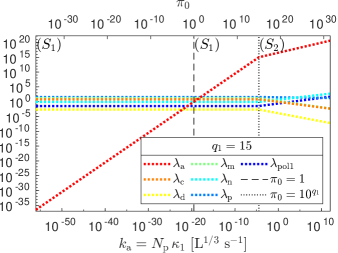
(a) Coefficients $\lambda$ (37) when $q_{1}=15$.

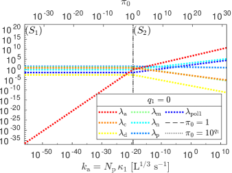
(b) Coefficients $\lambda$ (37) when $q_{1}=0$.

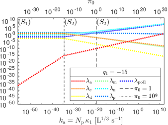
(c) Coefficients $\lambda$ (37) when $q_{1}=-15$.

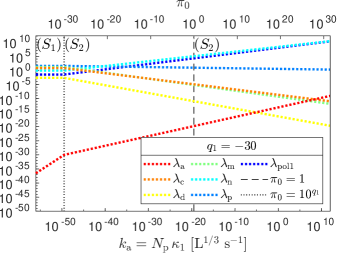
(d) Coefficients $\lambda$ (37) when $q_{1}=-30$.

Figure 2: Coefficients $\lambda(\tilde{\theta}^{N_{x}}_{\mathrm{opt}},\tilde{p})$ (37), with $\kappa_{1},\dots,\kappa_{7}$ defined in Table 1, $\tilde{p}=\tilde{p}_{\mathrm{exp}}$ given in Table 2, i.e. $N_{\mathrm{p}}=2.8\times 10^{17}$, and $q_{1}\in\mathbb{R}$. The black vertical dotted lines delimit the ranges of admissibility for solutions corresponding to $(S_{1})$ and $(S_{2})$ respectively, while the black vertical dashed lines correspond to $\pi_{0}=1$. The coefficients $\lambda$ (37) achieve the regime (15) when they arise from $(S_{1})$ and $\pi_{0}$ (35) is $<1$. The values of $k_{\mathrm{a}}$ are shown in $\mathrm{L}^{1/3}$ $\mathrm{s}^{-1}$, with $\mathrm{L}$ for Litres and $\mathrm{s}$ for seconds.

4 Approximate LPMF PBM

In this section we exploit the regime (15) to derive LPMF PBMReducing model complexity by means of the Optimal Scaling: Population Balance Model for latex particles morphology formation without integral terms, but with the capability to accurately approximate (1)-(13). We remark that the analysis presented in this section is also valid for the whole family of such models with parameters

$$a\leq 0,\quad 0<b<1,\quad v_{0}>0.$$ (38)

We show that in addition to the obvious computational advantages expected from the elimination of integral terms, for some choices of parameters $b$ within $0<b<1$, the approximate LPMF PBMReducing model complexity by means of the Optimal Scaling: Population Balance Model for latex particles morphology formation allows for uncoupling the computation of the time-dependent factors $\tilde{\varrho}_{\mathrm{d}}(t)$, $\tilde{\varrho}_{\mathrm{p}}(t)$ and $\tilde{\eta}_{0}(t)$ (3)-(4) from the solutions $m$ and $w$ to (1). As a result, several potential advantages are expected, such as improved computational performance and prospects for advancement of integration algorithms for solving the model.

4.1 Validation

When (15) holds, it is possible to consider, in the sense discussed in Section 3.1, the model (1)-(13) without integral terms, i.e. with $\lambda_{\mathrm{a}}=0$, as an approximation of the original model with very small $\alpha(v,u,t)$, $\forall v,u,t\in\mathbb{R}^{+}$.

However, such an approximation cannot be valid if the discarded terms, i.e. the Smoluchowski’s coagulation equation [16], undergo singularity formation at a finite time $T^{*}>0$. Several kinds of singular behaviour are shown in the literature. For instance, as reviewed in [17], solutions to coagulation equations may lose “mass” after a finite time $T^{*}$ by the formation of particles with “infinite size” (gelation phenomenon).

Another undesired situation is when solutions blow up to infinity at a finite time $T^{*}$, as a possible (but not necessary) consequence of their self-similarity [18]. If a finite-time singularity arises, the solution at times $t\geq T^{*}$ of the approximate model cannot provide an accurate approximation of the solution to (1), despite the choice of very small $\alpha(v,u,t)$, $\forall v,u,t\in\mathbb{R}^{+}$.

In the light of discussed singular behaviours, it is necessary to ground the approximation made by discarding the integral terms in (1). In particular, we want to exclude the possibility of such scenarios as finite-time gelation and blow-ups for the model (1)-(13) when (38) holds.

Gelation occurs through formation of particles with “infinite size”. Such a possibility can be excluded if the total sizes $C_{m}(t)$ and $C_{w}(t)$ produced by coagulation are finite $\forall t\in\mathbb{R}^{+}$ [19], i.e.

$$\begin{cases}C_{m}(t)&:=\int_{0}^{\infty}\!\int_{0}^{\infty}(v+u)\,\alpha(v,u,t)\,m(v,t)\,m(u,t)\,du\,dv<\infty,\quad\forall t\in\mathbb{R}^{+},\\ C_{w}(t)&:=\int_{0}^{\infty}\!\int_{0}^{\infty}(v+u)\,\alpha(v,u,t)\,w(v,t)\,w(u,t)\,du\,dv<\infty,\quad\forall t\in\mathbb{R}^{+}.\end{cases}$$ (39)

When $\alpha$ in (39) is given by (2) and $m,w$ are solutions to (1), one obtains

$$\begin{cases}C_{m}(t)&=2\tilde{\alpha}_{0}(t)\left[M^{1+a}(t)M^{0}(t)+M^{1}(t)M^{a}(t)\right],\quad\forall t\in\mathbb{R}^{+},\\ C_{w}(t)&=2\tilde{\alpha}_{0}(t)\left[W^{1+a}(t)W^{0}(t)+W^{1}(t)W^{a}(t)\right],\quad\forall t\in\mathbb{R}^{+},\end{cases}$$ (40)

where $M^{x}(t)=\int_{0}^{\infty}\!v^{x}\,m(v,t)\,dv$ and $W^{x}(t)=\int_{0}^{\infty}\!v^{x}\,w(v,t)\,dv$, $\forall x\in\mathbb{R}$, $\forall t\in\mathbb{R}^{+}$. With help of (38) and the boundedness of $\tilde{\alpha}_{0}(t)\in(0,\kappa_{\mathrm{a}}]$, $\kappa_{\mathrm{a}}<\infty$, $\forall t\in\mathbb{R}^{+}$ (Appendix A), we apply Proposition C.2 to obtain:

$$\begin{cases}C_{m}(t)&\leq 2\kappa_{\mathrm{a}}\,\left[(K^{1+a}_{m}+M^{1}(t))(K^{0}_{m}+M^{1}(t))+(K^{a}_{m}+M^{1}(t))M^{1}(t)\right],\quad\forall t\in[0,T],\\ C_{w}(t)&\leq 2\kappa_{\mathrm{a}}\,\left[(K^{1+a}_{w}+W^{1}(t))(K^{0}_{w}+W^{1}(t))+(K^{a}_{w}+W^{1}(t))W^{1}(t)\right],\quad\forall t\in[0,T],\end{cases}$$ (41)

where $K^{x}_{m},K^{x}_{w}<\infty$, $\forall x\in\mathbb{R}$, and $T$ can be arbitrary prescribed, as long as it is finite. Since the first-order moments $M^{1}(t)$ and $W^{1}(t)$ are finite for all time $t\in\mathbb{R}^{+}$ under (38) (see Proposition C.3 in Appendix C), equations (41) assure that finite-time gelation does not affect the solutions to the PBE system (1)-(13).

The same requirements on parameters $a$, $b$ and $v_{0}$, i.e. (38), allow us to show the boundedness of $m(v,t)$ and $w(v,t)$ when $v\in\mathbb{R}^{+}$, $t\in[0,T]$ and $T<\infty$ is an arbitrary fixed number (see Proposition D.1 in Appendix D), and thus to exclude the existence of the solutions $m,w$ to (1)-(13) which blow up to infinity at a finite time.

In conclusion, finite-time singularities do not emerge in the PBE system (1)-(13) and hence the approximation discarding the integral terms in (1) is valid.

Next it will be shown that if $(1-b)^{-1}\in\mathbb{N}$ (like, for example, in Table 1) then an approximate model can be simplified further through uncoupling the computation of time-dependent factors in (3)-(4) from the solutions $m$ and $w$ to (1). We shall call a model derived in such a way a LPMF PBMReducing model complexity by means of the Optimal Scaling: Population Balance Model for latex particles morphology formation of reduced complexity, or r-LPMF PBMReducing model complexity by means of the Optimal Scaling: Population Balance Model for latex particles morphology formation.

4.2 r-LPMF PBM

By setting $\alpha(v,u,t)\equiv 0$ in (1) one obtains:

$$\begin{cases}\partial_{t}m(v,t)&=-\,\partial_{v}\,(\,g(v,t)\,m(v,t)\,)\,+\,n(v,t)\,-\,\mu\,m(v,t),\quad\forall v,t\in\mathbb{R}^{+},\\ \partial_{t}w(v,t)&=-\,\partial_{v}\,(\,g(v,t)\,w(v,t)\,)\,+\,\mu\,m(v,t),\quad\forall v,t\in\mathbb{R}^{+},\\ m(v,0)&=w(v,0)=m(0,t)=w(0,t)=0,\quad\forall v,t\in\mathbb{R}^{+}.\end{cases}$$ (42)

Here the rates $g$, $n$ and $\mu$ in (42) are defined as before ((3)-(5)), i.e.

$$g(v,t)=\,\tilde{\varrho}_{\mathrm{d}}(t)\,v^{b}+\,\tilde{\varrho}_{\mathrm{p}}(t)\,v,\quad\tilde{\varrho}_{\mathrm{p}}(t)=\,\lambda_{\mathrm{p}}\,\frac{\Psi(t)}{V_{p}(t)},\quad\tilde{\varrho}_{\mathrm{d}}(t)=\,\lambda_{\mathrm{d}}\,\Phi(t)\,(\Psi(t)+1)^{2/3},\quad 0<b<1,$$ (43)

$$n(v,t)=\,\tilde{\eta}_{0}(t)\,\delta(v-v_{0}),\quad\tilde{\eta}_{0}(t)=\,\lambda_{\mathrm{n}}\,\Phi(t),\quad v_{0}=\lambda_{\mathrm{c}},\quad\mbox{with }\delta(x)\mbox{ the Dirac delta},$$ (44)

$$\mu=\lambda_{\mathrm{m}}.$$ (45)

The time-dependent functions $\Psi(t)$ and $\Phi(t)$ in (43)-(44) are computed as in (9)-(11):

$$\begin{cases}\frac{d\Psi(t)}{dt}&=-\lambda_{\mathrm{p}}\,\frac{\Psi(t)}{\Psi(t)+1}\,\frac{\Psi(t)+\Psi_{r}}{V_{\mathrm{pol2}}(t)+\lambda_{\mathrm{pol1}}},\quad\forall t\in\mathbb{R}^{+},\\ \frac{dV_{\mathrm{pol2}}(t)}{dt}&=\,\lambda_{\mathrm{p}}\,\frac{\Psi(t)}{\Psi(t)+1},\quad\forall t\in\mathbb{R}^{+},\\ \Psi(0)&=\,\bar{\Psi},\quad V_{\mathrm{pol2}}(0)=\,0,\end{cases}$$ (46)

$$\Phi(t)=\max\left\{\frac{V^{\mathrm{mat}}_{\mathrm{pol2}}(t)}{(\Psi(t)+1)(V^{\mathrm{mat}}_{\mathrm{pol2}}(t)+\lambda_{\mathrm{pol1}})}-\Phi_{s},0\right\},\quad\forall t\in\mathbb{R}^{+}.$$ (47)

The variable $V_{p}(t)$ in (43) can be expressed as (A.8) in Appendix A:

$$V_{p}(t)=\left(\Psi(t)+1\right)\left[V_{\mathrm{pol2}}(t)+\lambda_{\mathrm{pol1}}\right],\quad\forall t\in\mathbb{R}^{+},$$ (48)

and $V^{\mathrm{mat}}_{\mathrm{pol2}}(t)$ in (47) as (see (A.7) in Appendix A):

$$V^{\mathrm{mat}}_{\mathrm{pol2}}(t)=V_{\mathrm{pol2}}(t)-M^{1}(t)-W^{1}(t),\quad\forall t\in\mathbb{R}^{+},$$ (49)

where $M^{1}(t):=\int_{0}^{\infty}\!v\,m(v,t)\,dv$ and $W^{1}(t):=\int_{0}^{\infty}\!v\,w(v,t)\,dv$. We remark that (49) makes use of the equivalence between the variables $V^{\mathrm{c_{m}}}_{\mathrm{pol2}},V^{\mathrm{c_{w}}}_{\mathrm{pol2}}$ (7)-(8) and the first-order moments $M^{1},W^{1}$ of the solutions $m,w$ to (42). Such an equivalence is unveiled by integrating (42) times $v$ over $\mathbb{R}^{+}$ that leads to evolution equations equivalent to (7)-(8), i.e. the equations (53) at $x=1$, shown below.

If $M^{1},W^{1}$ in (49) are obtained by integration of $m,w$, the calculation of $\tilde{\varrho}_{\mathrm{d}}(t)$, $\tilde{\varrho}_{\mathrm{p}}(t)$ and $\tilde{\eta}_{0}(t)$ in (43)-(44) requires the knowledge of $m(v,t)$ and $w(v,t)$. However, it is possible to uncouple such a computation, as we show below. In particular, we aim to demonstrate that for specific values of a parameter $b$, $0<b<1$ and $(1-b)^{-1}\in\mathbb{N}$, the evolution equations of moments $M^{x},W^{x}$, $x=k\,(1-b)$ and $k=0,1,\dots,(1-b)^{-1}$ of solutions to (42) are closed-form ODE equations:

$$\begin{cases}\frac{d}{dt}M^{k(1-b)}(t)&=(k\,(1-b)\,\tilde{\varrho}_{\mathrm{p}}(t)-\mu)\,M^{k(1-b)}(t)\,+\,k\,(1-b)\,\tilde{\varrho}_{\mathrm{d}}(t)\,M^{(k-1)(1-b)}(t)\,+\\ &\quad\,+\,\tilde{\eta}_{0}(t)\,v_{0}^{k(1-b)},\quad k=0,1,\dots,(1-b)^{-1},\quad\forall t\in\mathbb{R}^{+},\\ \frac{d}{dt}W^{k(1-b)}(t)&=k\,(1-b)\,\tilde{\varrho}_{\mathrm{p}}(t)\,W^{k(1-b)}(t)\,+\,k\,(1-b)\,\tilde{\varrho}_{\mathrm{d}}(t)\,W^{(k-1)(1-b)}(t)\,+\\ &\quad\,+\,\mu\,M^{k(1-b)}(t),\quad k=0,1,\dots,(1-b)^{-1},\quad\forall t\in\mathbb{R}^{+},\\ M^{k(1-b)}(0)&=W^{k(1-b)}(0)=0,\quad k=0,1,\dots,(1-b)^{-1}.\end{cases}$$ (50)

Let us consider the evolution equations for the moments $M^{x}(t):=\int_{0}^{\infty}\!v^{x}\,m(v,t)\,dv$ and $W^{x}(t):=\int_{0}^{\infty}\!v^{x}\,w(v,t)\,dv$ with any fixed order $x>-b$, $0<b<1$, of solutions $m,w$ to (42):

$$\begin{cases}\frac{dM^{x}(t)}{dt}&=-\,\lim_{v\to\infty}\,g^{x}_{m}(v,t)\,+\,(x\tilde{\varrho}_{\mathrm{p}}(t)-\mu)\,M^{x}(t)\,+\,x\tilde{\varrho}_{\mathrm{d}}(t)\,M^{x+b-1}(t)\,+\,\tilde{\eta}_{0}(t)\,v_{0}^{x},\\ \frac{dW^{x}(t)}{dt}&=-\,\lim_{v\to\infty}\,g^{x}_{w}(v,t)\,+\,x\tilde{\varrho}_{\mathrm{p}}(t)\,W^{x}(t)\,+\,x\tilde{\varrho}_{\mathrm{d}}(t)\,W^{x+b-1}(t)\,+\,\mu\,M^{x}(t),\\ M^{x}(0)&=W^{x}(0)=0,\end{cases}$$ (51)

where

$$g^{x}_{y}(v,t):=(\tilde{\varrho}_{\mathrm{d}}(t)v^{x+b}+\tilde{\varrho}_{\mathrm{p}}(t)v^{x+1})\,y(v,t),\quad y=m,w.$$ (52)

First, we intend to show that $g^{x}_{m,w}(v,t)\to 0$ when $v\to\infty$, for any fixed $x\in\mathbb{R}$ and $t\in\mathbb{R}^{+}$, and thus equations (51) can be further simplified.

Following the derivation presented in Appendix D, one can demonstrate that the solution $m$ to (42) is (D.15) with $m(v,0)=\mathcal{I}_{m}(v,t)=0$, $\forall v\in\mathbb{R}$, $\forall t\in\mathbb{R}^{+}$, and a similar expression can be obtained for $w$. Then, it follows that the solutions $m(v,t)$ and $w(v,t)$ to (42) are equal to $0$ if $\varphi_{*}(t,v)>v_{0}$. Moreover, the condition $\varphi_{*}(t,v)>v_{0}$ is equivalent to $v=\varphi(t,\varphi_{*}(t,v))>\varphi(t,v_{0})$, due to $\varphi(t,v_{*})$ (D.5) being strictly increasing function of its second argument $v_{*}$ (see Appendix D). Thus, $m(v,t)=w(v,t)=0$ for all $v>\varphi(t,v_{0})$ at any fixed time $t\in\mathbb{R}^{+}$.

As discussed in Appendix D, the ODE (D.5) provides a well-defined (global) solution $\varphi(t,v_{0})<\infty$ and, hence, one obtains $\lim_{v\to\infty}v^{y}\,z(v,t)=0$ for $z=m,w$ with any fixed $y=x+b,x+1\in\mathbb{R}$ and $t\in\mathbb{R}^{+}$. Recalling that $\tilde{\varrho}_{\mathrm{d}},\tilde{\varrho}_{\mathrm{p}}$ are bounded functions of time $t$ (see Appendix A), we conclude that $g^{x}_{m,w}(v,t)\to 0$ as $v\to\infty$, for any fixed $x\in\mathbb{R}$ and $t\in\mathbb{R}^{+}$. This property allows for rewriting (51) as

$$\begin{cases}\frac{dM^{x}(t)}{dt}&=(x\tilde{\varrho}_{\mathrm{p}}(t)-\mu)\,M^{x}(t)\,+\,x\tilde{\varrho}_{\mathrm{d}}(t)\,M^{x+b-1}(t)\,+\,\tilde{\eta}_{0}(t)\,v_{0}^{x},\\ \frac{dW^{x}(t)}{dt}&=x\tilde{\varrho}_{\mathrm{p}}(t)\,W^{x}(t)\,+\,x\tilde{\varrho}_{\mathrm{d}}(t)\,W^{x+b-1}(t)\,+\,\mu\,M^{x}(t),\\ M^{x}(0)&=W^{x}(0)=0.\end{cases}$$ (53)

The ODE system (53) for $x=1$ is defined by the set of moments with orders $1$ and $1+j(b-1)$ for all integers $j\geq 1$ and, in general, is an infinite-dimensional system ($b-1\neq 0$). However, the dimensionality of such a system can be reduced to a finite value by $(i)$ exploiting the behaviour of (53) at $x=0$ and $(ii)$ restricting further the admissible values of $b$.

Let us consider first (53) for $x=0$. We notice that $\tilde{\eta}_{0}(t)$ in (53) depends on $M^{1}(t)$ and $W^{1}(t)$ through (44)-(49). Then the time derivatives of the zero-order moments $M^{0}(t)$ and $W^{0}(t)$ are functions of the moments of orders $0$ and $1$ only. In particular, since $x=0$ in (53), the moments of order $b-1<0$ vanish (here we use the finiteness of function $\tilde{\varrho}_{\mathrm{d}}(t)$ and PBE solutions’ moments shown in Appendix A and Appendix C respectively).

When $x=1$ the moments $M^{0}(t)$ and $W^{0}(t)$ can appear in (53) only if there exists an integer $j\geq 1$ such that $1+j(b-1)=0$, i.e. if $(1-b)^{-1}\in\mathbb{N}$. In this case the number of state variables of the ODE system (53) is not infinite anymore. In particular, the ODE system state is the finite set of moments $M^{y}(t)$ and $W^{y}(t)$, with $y=1+j(b-1),1$ and integer $j=1,\dots,(1-b)^{-1}$. This is because, when $j=(1-b)^{-1}\in\mathbb{N}$, i.e. $y=0$, the time derivatives of $M^{0}(t)$ and $W^{0}(t)$ depend only on variables already belonging to the state of the ODE system, i.e. the moments of orders $0$ and $1$.

Finally, we notice that such a finite-dimensional ODE system corresponds to (50). We also remark that the ODE system (50) is written in a closed-form. Indeed, the only unknowns in the RHS of (50) are the moments $M^{k(1-b)}(t)$ and $W^{k(1-b)}(t)$, with $k=0,1,\dots,(1-b)^{-1}$, whose time derivatives constitute the LHS of (50). In particular, the moments of order $(k-1)(1-b)$ are cancelled out when $k=0$.

Once coupled with (43)-(49), the ODE system (50) can be integrated numerically in time. Such a numerical solution provides the values of moments $M^{1}(t)$ and $W^{1}(t)$ (when $k=(1-b)^{-1}\in\mathbb{N}$) required for the calculation of $\tilde{\varrho}_{\mathrm{d}}(t)$, $\tilde{\varrho}_{\mathrm{p}}(t)$ and $\tilde{\eta}_{0}(t)$ (43)-(44), without the need for accessing values of densities $m(v,t)$ and $w(v,t)$.

In conclusion, we have derived the r-LPMF PBMReducing model complexity by means of the Optimal Scaling: Population Balance Model for latex particles morphology formation (42)-(50) whose coefficients are defined in Table 1 and Table 2. Such a model approximates the LPMF PBMReducing model complexity by means of the Optimal Scaling: Population Balance Model for latex particles morphology formation (1)-(13) under the coefficients’ regime (15). When $a\leq 0$, $0<b<1$, $(1-b)^{-1}\in\mathbb{N}$, $v_{0}>0$, the r-LPMF PBMReducing model complexity by means of the Optimal Scaling: Population Balance Model for latex particles morphology formation offers a significant reduction in model complexity compared with its predecessor LPMF PBMReducing model complexity by means of the Optimal Scaling: Population Balance Model for latex particles morphology formation. In particular, it avoids the computation of integral terms, while allows for uncoupling the computation of functions $\tilde{\varrho}_{\mathrm{d}}(t)$, $\tilde{\varrho}_{\mathrm{p}}(t)$ and $\tilde{\eta}_{0}(t)$ from the solutions to the PBE of interest.

5 Numerical Testing

Our next objectives are $(i)$ to provide numerical evidence for the feasibility and accuracy of the approximation discussed above and $(ii)$ to investigate the advantages of the r-LPMF PBMReducing model complexity by means of the Optimal Scaling: Population Balance Model for latex particles morphology formation over the LPMF PBMReducing model complexity by means of the Optimal Scaling: Population Balance Model for latex particles morphology formation. Though the r-LPMF PBMReducing model complexity by means of the Optimal Scaling: Population Balance Model for latex particles morphology formation represents the family of models with $a\leq 0$, $0<b<1$ and $(1-b)^{-1}\in\mathbb{N}$, up to now, only the model (1)-(13) with $a=-1/3$ and $b=2/3$ was physically supported [7, 9]. Therefore, we limit our tests to this particular model and the corresponding approximate model (42)-(50) with $b=2/3$. Moreover, we employ the physically grounded values of $\bar{\Psi}$, $\Psi_{r}$ and $\Phi_{s}$ provided in Table 1.

We use the GMOC method [9] for computing numerical solutions to the PBE systems (1)-(5) and (42)-(45). The Runge-Kutta method (RK4) [20] is applied to integrate in time the ODE systems (6)-(13) and (46)-(50). As suggested in [9], the pointwise evaluation of the function $n(v,t)$ in (4) and (44) relies on the approximation

$$\delta(v-v_{0})\approx\mathcal{N}(v;v_{0},\sigma_{0}),\quad\forall v\in\mathbb{R},\quad v_{0}\gg\sigma_{0}>0,$$ (54)

where $\mathcal{N}(x;x_{0},s_{0})$ denotes the probability density function at $x\in\mathbb{R}$ of a Gaussian random variable with mean $x_{0}\in\mathbb{R}$ and standard deviation $s_{0}>0$.

5.1 Feasibility and Accuracy of r-LPMF PBM

As discussed in Section 4, the r-LPMF PBMReducing model complexity by means of the Optimal Scaling: Population Balance Model for latex particles morphology formation (42)-(50) is derived by exploiting the regime (15) of coefficients $\lambda$ (14) defined in Table 1. Given $a=-1/3$ and $b=2/3$ from Table 1, Section 3.3 provides a condition on physical parameters to meet (15). Specifically, the regime (15) can be achieved when the following inequality holds:

$$\pi_{0}<1,\quad\mbox{with}\quad\pi_{0}\quad\mbox{defined as}\quad\eqref{eqn:Pi_a_def}\quad\mbox{when}\quad a=-1/3\quad\mbox{and}\quad b=2/3.$$ (55)

Therefore, we expect the solutions of the LPMF PBMReducing model complexity by means of the Optimal Scaling: Population Balance Model for latex particles morphology formation (1)-(13) to be reproduced by the r-LPMF PBMReducing model complexity by means of the Optimal Scaling: Population Balance Model for latex particles morphology formation (42)-(50) when the parameters from Table 2 satisfy (55).

First, we verify such a statement for the parameters $\tilde{p}=\tilde{p}_{\mathrm{exp}}$ given in Table 2 and a set of the aggregation rate $k_{\mathrm{a}}$’s values. Since $\pi_{0}\propto k_{\mathrm{a}}$ (see (35) and Table 1), decreasing values of $k_{\mathrm{a}}$ ultimately will lead to $\pi_{0}<1$, i.e. a slow aggregation, while increasing values of $k_{\mathrm{a}}$ will give $\pi_{0}\geq 1$, i.e. fast aggregation. In agreement, Figure 3 shows that the solutions $m(v,t)$ and $w(v,t)$ of the r-LPMF PBMReducing model complexity by means of the Optimal Scaling: Population Balance Model for latex particles morphology formation (first column from the left) are indistinguishable from the solutions of the LPMF PBMReducing model complexity by means of the Optimal Scaling: Population Balance Model for latex particles morphology formation with aggregation rates $k_{\mathrm{a}}$ leading to $\pi_{0}<1$ ($k_{\mathrm{a}}$ and $\pi_{0}$ in green). On the other hand, a difference is appreciable for larger $k_{\mathrm{a}}$ giving $\pi_{0}\geq 1$ ($k_{\mathrm{a}}$ and $\pi_{0}$ in red).

In order to quantify the deviation between compared solutions, we define the metric

$$e_{y}(t):=\frac{\max_{v}|y_{\mbox{\footnotesize{LPMF}}}(v,t)-y_{\mbox{\footnotesize{r-LPMF}}}(v,t)|}{\max_{v}|y_{\mbox{\footnotesize{r-LPMF}}}(v,t)|},\quad y=m,w,\quad\forall t\in\mathbb{R}^{+},$$ (56)

where $y_{\mbox{\footnotesize{LPMF}}},y_{\mbox{\footnotesize{r-LPMF}}}$ correspond to solutions either $m$ or $w$ of the models LPMF (1)-(13) and r-LPMF (42)-(50) respectively.

Figure 4 demonstrates that the relative approximation errors $e_{m},e_{w}$ (56) are reduced when aggregation rates $k_{\mathrm{a}}$ and, thus, $\pi_{0}\propto k_{\mathrm{a}}$ decrease. In particular, values of $k_{\mathrm{a}}$ corresponding to $\pi_{0}<1$ ensure $e_{m}(t),e_{w}(t)\lesssim 10^{-3}$ for all tested times $t$. We remark that the chosen range of simulated times $t$ allows for monitoring the dynamical processes accounted by the r-LPMF PBMReducing model complexity by means of the Optimal Scaling: Population Balance Model for latex particles morphology formation up to the point when solutions $m$ and $w$ reach stationary states (see first column from the left in Figure 3). Computational settings and parameter values are reported in Table 3.

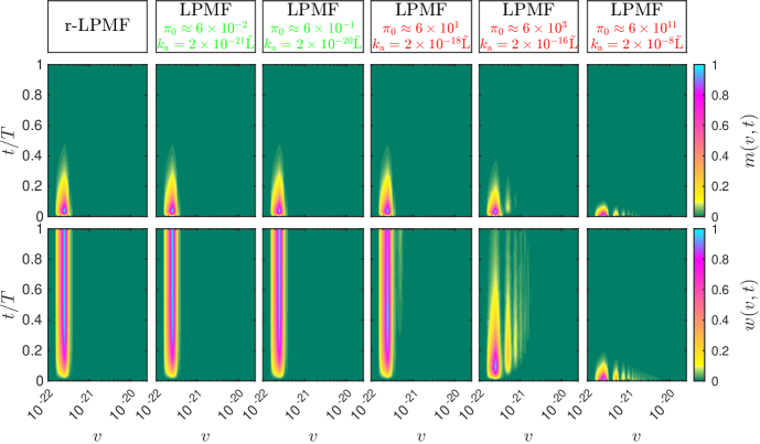
Figure 3: Solutions $m(v,t)$ and $w(v,t)$ of the r-LPMF PBM (42)-(50) (left column) and the LPMF PBM(1)-(13), with coefficients $\lambda(\theta,\tilde{p})$ (Table 1), $\theta=\{\nu_{0},t_{0},d_{0}\}$, $\nu_{0}=1/d_{0}=1\,\mathrm{L}$, $t_{0}=1\,\mathrm{s}$ and $\tilde{p}=\tilde{p}_{\mathrm{exp}}$ (Table 2). The values of $k_{\mathrm{a}}$ are chosen in such a way that both scenarios, $(i)$ $\pi_{0}$ (35) $<1$ ($k_{\mathrm{a}}$ and $\pi_{0}$ are shown in green) and $(ii)$ $\pi_{0}\geq 1$ ($k_{\mathrm{a}}$ and $\pi_{0}$ in red), are present. The tested values of $k_{\mathrm{a}}$ are reported in $\tilde{\mathrm{L}}:=\mathrm{L}^{1/3}\,\mathrm{s}^{-1}$. The shown $y=m,w$ are scaled as $y(v,t)\leftarrow[y(v,t)-\min_{v,t}y(v,t)]/[\max_{v,t}y(v,t)-\min_{v,t}y(v,t)]$, whereas the time $t$ is normalized to $T=10^{6}$. Computational settings and parameter values are detailed in Table 3.

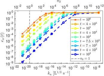
Figure 4: Dependence of the metric $e_{y}(t)$ (56), for $y=m$ (left) and $y=w$ (right), on the aggregation rate $k_{\mathrm{a}}$ (Table 2) and, thus, $\pi_{0}$ (35) $\propto k_{\mathrm{a}}$ (see Table 1). Values of $k_{\mathrm{a}}$ leading to $\pi_{0}<1$ ensure $e_{m}(t),e_{w}(t)\lesssim 10^{-3}$ for all tested times $t$. The plots show $k_{\mathrm{a}}$ in $\mathrm{L}^{1/3}$ $\mathrm{s}^{-1}$, while the remaining physical parameters are provided in Table 2. Computational settings and parameter values are reported in Table 3.

	LPMF PBMReducing model complexity by means of the Optimal Scaling: Population Balance Model for latex particles morphology formation	r-LPMF PBMReducing model complexity by means of the Optimal Scaling: Population Balance Model for latex particles morphology formation
PBE	(1)-(5)	(42)-(45)
ODE	(6)-(13)	(46)-(50)
Coefficients $\lambda$	$\lambda=\lambda(\theta,\tilde{p})$ (Table 1), $\theta=\{\nu_{0},t_{0},d_{0}\}$
	$\nu_{0}=1/d_{0}=1\,\mathrm{L}$, $t_{0}=1\,\mathrm{s}$
Parameters $\tilde{p}$	Figures 3-4: $\tilde{p}=\tilde{p}_{\mathrm{exp}}$ (Table 2)
	Figures 5-6: $\tilde{p}$ set as (57)
	Figures 7-8: $\tilde{p}$ set as (58)
	Figures 9-10: $\tilde{p}$ set as (59)
PBE solver	GMOC [9] with (54) and $\sigma_{0}=v_{0}/10$
ODE solver	Runge-Kutta (RK4) [20]
Volume Grid v	$\textbf{v}=\{kh\}_{k=0}^{N}$, $h=V/N$, $V=10^{2}\,v_{0}$, $N=10^{3}$
Time Grid t	$\textbf{t}=\{k\tau\}_{k=0}^{M}$, $\tau=T/M$
	Figures 3-4: $T=10^{6}$, $M=5\times 10^{5}$
	Figures 5-6: $T=5\times 10^{5}$, $M=5\times 10^{5}$
	Figures 7-8: $T=10^{6}$, $M=10^{6}$
	Figures 9-10: $T=10^{6}$, $M=5\times 10^{5}$
SW/HW	C++ BCAM code, 64-bit Linux OS, 2.40GHz proc.

Table 3: Computational settings and parameter values for integration of the LPMF PBM (1)-(13) and r-LPMF PBM (42)-(50) within the volume domain $[0,V]$ and the time interval $[0,T]$. The resulting solutions and relative errors (56) are shown in Figures 3-10. The scaling factors $\theta$ are reported in Litres [$\mathrm{L}$] and seconds [$\mathrm{s}$]. SW/HW stands for Software & Hardware, while BCAM code refers to the in-house package.

In what follows, we provide further evidence that the inequality $\pi_{0}<1$ (55) can serve as a quantitative criterion for the feasibility of r-LPMF PBMReducing model complexity by means of the Optimal Scaling: Population Balance Model for latex particles morphology formation. In particular, we verify that the solutions of LPMF PBMReducing model complexity by means of the Optimal Scaling: Population Balance Model for latex particles morphology formation can be reproduced by the r-LPMF PBMReducing model complexity by means of the Optimal Scaling: Population Balance Model for latex particles morphology formation, when the condition (55) is met by parameters $\tilde{p}$ that take values in a broader range than the one proposed in Table 2. More specifically, sets of $k_{\mathrm{d}}$, $k_{\mathrm{n}}$ and $v_{\mathrm{c}}$’s values are explored.

The first experiment considers the transport rate $k_{\mathrm{d}}$ ranging in the interval

$$k_{\mathrm{d}}\in[10^{-17},2\times 10^{-10}]\,\tilde{\mathrm{L}},\quad\mbox{with the fixed}\quad k_{\mathrm{a}}=2\times 10^{-16}\,\tilde{\mathrm{L}}$$ (57)

$$\mbox{and the remaining}\quad\tilde{p}=\tilde{p}_{\mathrm{exp}}\quad\mbox{as defined in \autoref{tab:p_exp_def}},$$

where $\tilde{\mathrm{L}}:=\mathrm{L}^{1/3}\,\mathrm{s}^{-1}$. Figure 5 compares the LPMF PBMReducing model complexity by means of the Optimal Scaling: Population Balance Model for latex particles morphology formation and r-LPMF PBMReducing model complexity by means of the Optimal Scaling: Population Balance Model for latex particles morphology formation solutions, indicating in red and green the values of $k_{\mathrm{d}}$ leading to $\pi_{0}\geq 1$ and $\pi_{0}<1$ respectively.

Since $\pi_{0}\propto k_{\mathrm{d}}^{-13/16}$ (see (35) and Table 1), it follows that $\pi_{0}\geq 1$, i.e. a regime of fast aggregation, can be achieved by decreasing values of $k_{\mathrm{d}}$. Indeed, we observe that the LPMF PBMReducing model complexity by means of the Optimal Scaling: Population Balance Model for latex particles morphology formation and r-LPMF PBMReducing model complexity by means of the Optimal Scaling: Population Balance Model for latex particles morphology formation solutions compared in Figure 5 are quite different when $\pi_{0}\geq 1$ ($k_{\mathrm{d}}$ and $\pi_{0}$ in red).

On the other hand, a larger $k_{\mathrm{d}}$ promotes the transport process in such a way that aggregation has a lower importance in the overall dynamics of LPMF PBMReducing model complexity by means of the Optimal Scaling: Population Balance Model for latex particles morphology formation solutions. Figure 5 shows that the condition $\pi_{0}<1$ allows detecting regimes of moderate aggregation, when $\tilde{p}$ are set as in (57).

These observations can be quantified by the relative errors (56) between LPMF PBM and r-LPMF PBM solutions compared in Figure 5. In particular, Figure 6 shows that the difference (56) can be decreased by enlarging $k_{\mathrm{d}}$ to meet $\pi_{0}<1$ (55). The approximation errors span the range of magnitudes from $10^{-4}$ to $10^{0}$ when polymerization time increases from $\approx 17$ min to $\approx 139$ hours.

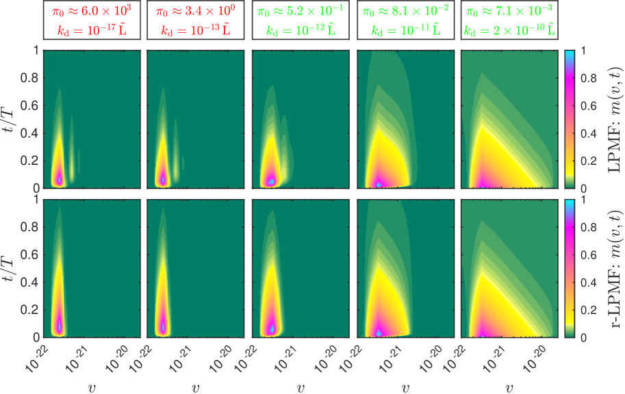
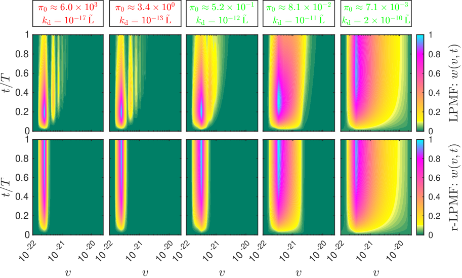
Figure 5: Solutions $m(v,t)$ and $w(v,t)$ of the r-LPMF PBM (42)-(50) and the LPMF PBM (1)-(13), with coefficients $\lambda(\theta,\tilde{p})$ (Table 1), $\theta=\{\nu_{0},t_{0},d_{0}\}$, $\nu_{0}=1/d_{0}=1\,\mathrm{L}$, $t_{0}=1\,\mathrm{s}$ and $\tilde{p}$ given as (57). The values of $k_{\mathrm{d}}$ are chosen in such a way that both scenarios, $(i)$ $\pi_{0}$ (35) $<1$ ($k_{\mathrm{d}}$ and $\pi_{0}$ are shown in green) and $(ii)$ $\pi_{0}\geq 1$ ($k_{\mathrm{d}}$ and $\pi_{0}$ in red), are present. The plot provides $k_{\mathrm{d}}$ in $\tilde{\mathrm{L}}:=\mathrm{L}^{1/3}\,\mathrm{s}^{-1}$. The shown $y=m,w$ are scaled as $y(v,t)\leftarrow[y(v,t)-\min_{v,t}y(v,t)]/[\max_{v,t}y(v,t)-\min_{v,t}y(v,t)]$, whereas the time $t$ is normalized to $T=5\times 10^{5}$. Computational settings and parameter values are detailed in Table 3.

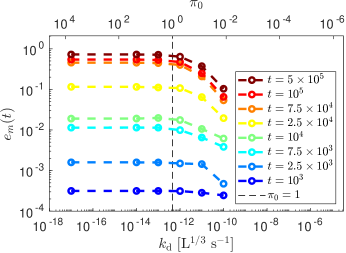
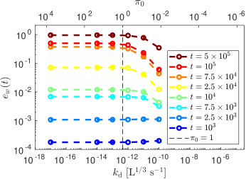
Figure 6: Metric $e_{y}(t)$ (56), with $y=m$ (left) and $y=w$ (right), versus transport rate $k_{\mathrm{d}}$. The quantity $\pi_{0}$ (35) decreases with increasing $k_{\mathrm{d}}$, i.e. $\pi_{0}\propto k_{\mathrm{d}}^{-13/16}$ (see (35) and Table 1). The errors $e_{m},e_{w}$ can be reduced by enlarging $k_{\mathrm{d}}$ to meet $\pi_{0}<1$. The plots provide $k_{\mathrm{d}}$ in $\mathrm{L}^{1/3}$ $\mathrm{s}^{-1}$, while the remaining physical parameters are presented in (57). Computational settings and parameter values are reported in Table 3.

Next, we consider the nucleation rate $k_{\mathrm{n}}$ assuming values in the interval

$$k_{\mathrm{n}}\in[2.5\times 10^{-17},2.5\times 10^{-5}]\,\mathrm{L}\,\mathrm{s}^{-1},\quad\mbox{with the fixed}\quad k_{\mathrm{a}}=2\times 10^{-16}\,\mathrm{L}^{1/3}\,\mathrm{s}^{-1},$$ (58)

$$\mbox{and the remaining}\quad\tilde{p}=\tilde{p}_{\mathrm{exp}}\quad\mbox{as defined in \autoref{tab:p_exp_def}}.$$

Figure 7 compares solutions of the LPMF PBMReducing model complexity by means of the Optimal Scaling: Population Balance Model for latex particles morphology formation and r-LPMF PBMReducing model complexity by means of the Optimal Scaling: Population Balance Model for latex particles morphology formation corresponding to a set of physical parameters chosen as in (58). The values of $k_{\mathrm{n}}$ leading to $\pi_{0}\geq 1$ (in red) result in the significant deviation of the LPMF PBMReducing model complexity by means of the Optimal Scaling: Population Balance Model for latex particles morphology formation solutions from the corresponding r-LPMF PBMReducing model complexity by means of the Optimal Scaling: Population Balance Model for latex particles morphology formation solutions. On the contrary, when $k_{\mathrm{n}}$ satisfies $\pi_{0}<1$ (in green), it is not possible to spot any visual difference between LPMF PBMReducing model complexity by means of the Optimal Scaling: Population Balance Model for latex particles morphology formation and r-LPMF PBMReducing model complexity by means of the Optimal Scaling: Population Balance Model for latex particles morphology formation solutions. This confirms that the inequality $\pi_{0}<1$ is a reliable threshold for detecting regimes of slow aggregation.

Figure 8 illustrates how the relative errors (56) vary with respect to the nucleation rate $k_{\mathrm{n}}$ (58). In particular, the difference between LPMF PBMReducing model complexity by means of the Optimal Scaling: Population Balance Model for latex particles morphology formation and r-LPMF PBMReducing model complexity by means of the Optimal Scaling: Population Balance Model for latex particles morphology formation solutions decreases with reducing $k_{\mathrm{n}}$ and, consequently, $\pi_{0}$, since $\pi_{0}\propto k_{\mathrm{n}}^{1/2}$ (see (35) and Table 1).

Finally, we perform an experiment by assuming the nucleation size $v_{\mathrm{c}}$ ranging in

$$v_{\mathrm{c}}\in[2.5\times 10^{-22},2.5\times 10^{-16}]\,\mathrm{L},\quad\mbox{with the fixed}\quad k_{\mathrm{a}}=2\times 10^{-16}\,\mathrm{L}^{1/3}\,\mathrm{s}^{-1},$$ (59)

$$\mbox{and the remaining}\quad\tilde{p}=\tilde{p}_{\mathrm{exp}}\quad\mbox{as defined in \autoref{tab:p_exp_def}}.$$

Figure 9 compares solutions of the LPMF PBMReducing model complexity by means of the Optimal Scaling: Population Balance Model for latex particles morphology formation and r-LPMF PBMReducing model complexity by means of the Optimal Scaling: Population Balance Model for latex particles morphology formation, showing that they are indistinguishable when $v_{\mathrm{c}}$ (59) gives $\pi_{0}<1$ ($v_{\mathrm{c}}$ and $\pi_{0}$ in green). In addition, Figure 10 provides the relative difference (56) as a function of $v_{\mathrm{c}}$ (59) or $\pi_{0}$ (35). Since $\pi_{0}\propto v_{\mathrm{c}}^{-17/16}$ (see (35) and Table 1), the approximation error (56) is reduced by increasing $v_{\mathrm{c}}$ and, thus, decreasing $\pi_{0}$.

In conclusion, we have validated that the inequality (55) can successfully serve as a criterion for applicability of the approximate model r-LPMF PBMReducing model complexity by means of the Optimal Scaling: Population Balance Model for latex particles morphology formation. Indeed, our experiments indicate that (55) can predict ranges of parameters promoting slow aggregation and, thus, the conditions when it is feasible to neglect the integral terms in the LPMF PBMReducing model complexity by means of the Optimal Scaling: Population Balance Model for latex particles morphology formation. We remark that (55) can be checked prior to modelling with minimal computational effort.

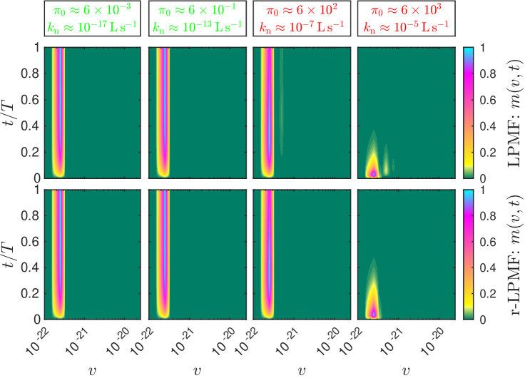
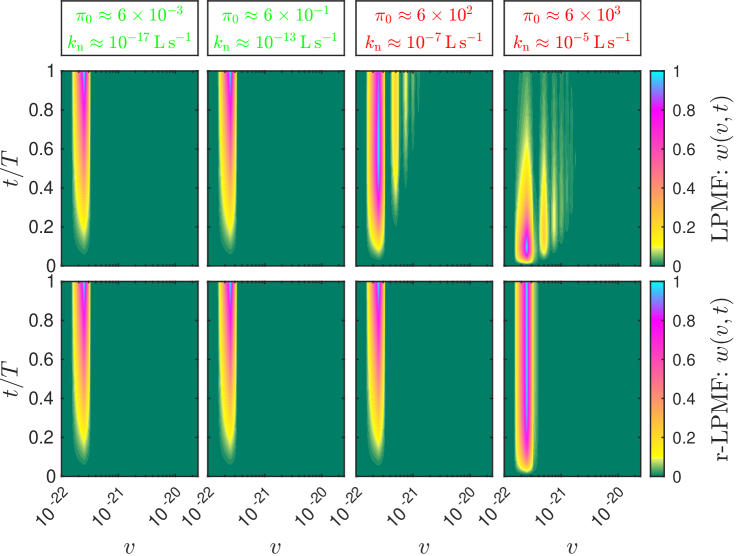
Figure 7: Solutions $m(v,t)$ and $w(v,t)$ of the r-LPMF PBM (42)-(50) and the LPMF PBM (1)-(13), with coefficients $\lambda(\theta,\tilde{p})$ (Table 1), $\theta=\{\nu_{0},t_{0},d_{0}\}$, $\nu_{0}=1/d_{0}=1\,\mathrm{L}$, $t_{0}=1\,\mathrm{s}$ and $\tilde{p}$ given as (58). The values of $k_{\mathrm{n}}$ are chosen in such a way that both scenarios, $(i)$ $\pi_{0}$ (35) $<1$ ($k_{\mathrm{n}}$ and $\pi_{0}$ are shown in green) and $(ii)$ $\pi_{0}\geq 1$ ($k_{\mathrm{n}}$ and $\pi_{0}$ in red), are present. The shown $y=m,w$ are scaled as $y(v,t)\leftarrow[y(v,t)-\min_{v,t}y(v,t)]/[\max_{v,t}y(v,t)-\min_{v,t}y(v,t)]$, whereas the time $t$ is normalized to $T=10^{6}$. Computational settings and parameter values are detailed in Table 3.

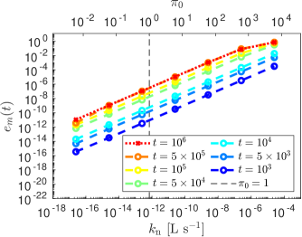
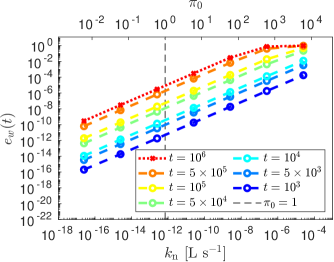
Figure 8: Metric $e_{y}(t)$ (56), with $y=m$ (left) and $y=w$ (right), versus nucleation rate $k_{\mathrm{n}}$. The dimensionless quantity $\pi_{0}$ (35) is directly proportional to $k_{\mathrm{n}}$, i.e. $\pi_{0}\propto k_{\mathrm{n}}^{1/2}$ (see (35) and Table 1). The plots provide $k_{\mathrm{n}}$ in $\mathrm{L}$ $\mathrm{s}^{-1}$, while the remaining physical parameters are set in (58). Computational settings and parameter values are reported in Table 3.

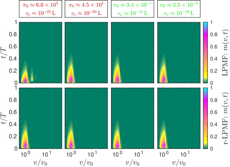
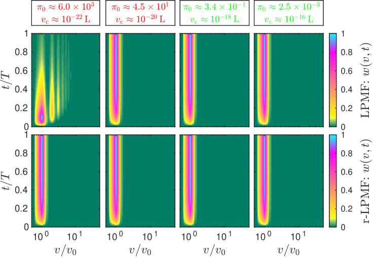
Figure 9: Solutions $m(v,t)$ and $w(v,t)$ of the r-LPMF PBM (42)-(50) and the LPMF PBM(1)-(13), with coefficients $\lambda(\theta,\tilde{p})$ (Table 1), $\theta=\{\nu_{0},t_{0},d_{0}\}$, $\nu_{0}=1/d_{0}=1\,\mathrm{L}$, $t_{0}=1\,\mathrm{s}$ and $\tilde{p}$ given as (59). The values of $v_{\mathrm{c}}$ are chosen in such a way that both scenarios, $(i)$ $\pi_{0}$ (35) $<1$ ($v_{\mathrm{c}}$ and $\pi_{0}$ are shown in green) and $(ii)$ $\pi_{0}\geq 1$ ($v_{\mathrm{c}}$ and $\pi_{0}$ in red), are present. The shown $y=m,w$ are scaled as $y(v,t)\leftarrow[y(v,t)-\min_{v,t}y(v,t)]/[\max_{v,t}y(v,t)-\min_{v,t}y(v,t)]$, whereas the volume $v$ and time $t$ are normalized to $v_{0}=v_{\mathrm{c}}/\nu_{0}$ and $T=10^{6}$ respectively. Computational settings and parameter values are detailed in Table 3.

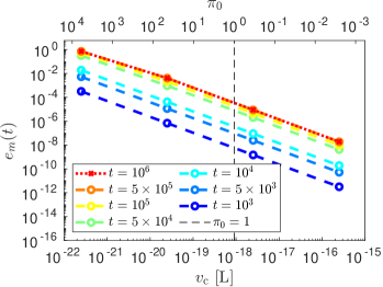
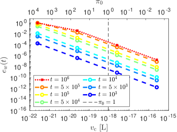
Figure 10: Metric $e_{y}(t)$ (56), with $y=m$ (left) and $y=w$ (right), versus nucleation size $v_{\mathrm{c}}$ shown in Litres [$\mathrm{L}$]. The remaining physical parameters are provided in (59). The dimensionless quantity $\pi_{0}$ (35) is inversely proportional to $v_{\mathrm{c}}$, i.e. $\pi_{0}\propto v_{\mathrm{c}}^{-17/16}$ (see (35) and Table 1). Computational settings and parameter values are reported in Table 3.

5.2 Computational Efficiency of the r-LPMF PBM

Lastly, we investigate the computational advantages of the r-LPMF PBMReducing model complexity by means of the Optimal Scaling: Population Balance Model for latex particles morphology formation over the LPMF PBMReducing model complexity by means of the Optimal Scaling: Population Balance Model for latex particles morphology formation. In particular, we compare the computational times required by the scaled r-LPMF PBMReducing model complexity by means of the Optimal Scaling: Population Balance Model for latex particles morphology formation and LPMF PBMReducing model complexity by means of the Optimal Scaling: Population Balance Model for latex particles morphology formation models to obtain “a true solution”. Here “a true solution” is generated by the original unscaled LPMF PBMReducing model complexity by means of the Optimal Scaling: Population Balance Model for latex particles morphology formation run for a long time with the safe choices of time and volume step sizes. The choices of simulation parameters for such runs were carefully verified. The performed experiments make use of parameters $\tilde{p}=\hat{p}_{\mathrm{exp}}$,

$$\hat{p}_{\mathrm{exp}}:=\tilde{p}_{\mathrm{exp}}\quad\mbox{(\autoref{tab:p_exp_def})},\quad\mbox{with}\quad k_{\mathrm{a}}=2\times 10^{-20}\,\mathrm{L}^{1/3}\,\mathrm{s}^{-1}.$$ (60)

Such a choice of parameters (60) allows discarding the integral terms in (1)-(13) without a substantial loss of accuracy (see Figures 3-4 in Section 5.1).

The first experiment consists in monitoring relative errors and required computational times, while the volume grid size $N$ is increased and the time grid size $M$ is fixed (see Table 4 for values of $N$ and $M$). We take as a reference the solutions of the unscaled LPMF PBMReducing model complexity by means of the Optimal Scaling: Population Balance Model for latex particles morphology formation (see description below (62)) computed with a volume grid size $N=N_{\mathrm{ref}}$ (see Table 4). Then, the relative errors between compared solutions are estimated as

$$\varepsilon^{y}_{X}(N):=\frac{\max_{v}|y_{X}^{N}(v,T)-y_{Z}^{N_{\mathrm{ref}}}(v,T)|}{\max_{v}|y_{Z}^{N_{\mathrm{ref}}}(v,T)|},\quad Z=\mbox{\footnotesize{unscaled LPMF PBM\ref{foot:1LPMFPBM}}},$$ (61)

where $y_{X}^{N}(v,T)$ is the solution $y=m,w$ at volume $v$ and time $t=T$ (see Table 4) of a model $X$ integrated by using a volume grid with size $N$. The models considered in (61) are labeled as

$$X=\begin{cases}\mbox{scaled LPMF PBM\ref{foot:1LPMFPBM}:}&\mbox{\eqref{eqn:PBE_latex}-\eqref{eqn:Sigma_m,w}, $\lambda=\lambda(\tilde{\theta}^{N_{x}}_{\mathrm{opt}},\tilde{p})$ \eqref{eqn:lambdas_computed_OSC}, $q_{1}=0$, $\tilde{p}=\hat{p}_{\mathrm{exp}}$ \eqref{eqn:hat_p_exp_def}},\\ \mbox{scaled r-LPMF PBM\ref{foot:5rLPMFPBM}:}&\mbox{\eqref{eqn:PBE_latex_approx}-\eqref{eqn:ODE_M,Wx_PBE_latex_no_IT_x=k(1-b)}, $\lambda=\lambda(\tilde{\theta}^{N_{x}}_{\mathrm{opt}},\tilde{p})$ \eqref{eqn:lambdas_computed_OSC}, $q_{1}=0$, $\tilde{p}=\hat{p}_{\mathrm{exp}}$ \eqref{eqn:hat_p_exp_def}}.\end{cases}$$ (62)

The unscaled LPMF PBMReducing model complexity by means of the Optimal Scaling: Population Balance Model for latex particles morphology formation model or $Z$ is defined in (1)-(13), with $\lambda=\lambda(\theta,\tilde{p})$ (Table 1), $\theta=\theta_{\mathrm{unit}}$ (Table 4) and $\tilde{p}=\hat{p}_{\mathrm{exp}}$ (60). Solutions $y_{Z}^{N_{\mathrm{ref}}}(v,T)$ in (61) are suitably scaled.

Figure 11 shows relative errors $\varepsilon^{m,w}_{X}(N)$ (61) and computational times required by the scaled LPMF PBMReducing model complexity by means of the Optimal Scaling: Population Balance Model for latex particles morphology formation and r-LPMF PBMReducing model complexity by means of the Optimal Scaling: Population Balance Model for latex particles morphology formation, while Table 4 reports computational settings and parameter values. If $N\lesssim 2\times 10^{2}$, the scaled r-LPMF PBMReducing model complexity by means of the Optimal Scaling: Population Balance Model for latex particles morphology formation and LPMF PBMReducing model complexity by means of the Optimal Scaling: Population Balance Model for latex particles morphology formation show almost identical errors. This confirms the negligible role of aggregation in the simulated process (see 11(a)). In addition, achieving such a level of accuracy requires up to an order of magnitude smaller computational time for r-LPMF PBMReducing model complexity by means of the Optimal Scaling: Population Balance Model for latex particles morphology formation than it is needed by LPMF PBMReducing model complexity by means of the Optimal Scaling: Population Balance Model for latex particles morphology formation (see 11(b)). Thus, if $N\lesssim 2\times 10^{2}$, replacing LPMF PBMReducing model complexity by means of the Optimal Scaling: Population Balance Model for latex particles morphology formation with r-LPMF PBMReducing model complexity by means of the Optimal Scaling: Population Balance Model for latex particles morphology formation improves the computational efficiency by up to an order of magnitude. Moreover, 11(b) indicates that the computational time required by LPMF PBMReducing model complexity by means of the Optimal Scaling: Population Balance Model for latex particles morphology formation increases quadratically when $N\to\infty$, i.e. it is $O(N^{2})$, while the r-LPMF PBMReducing model complexity by means of the Optimal Scaling: Population Balance Model for latex particles morphology formation’s cost scales as $O(N)$ for large $N$.

For $N>2\times 10^{2}$, the accuracy achieved by the scaled r-LPMF PBMReducing model complexity by means of the Optimal Scaling: Population Balance Model for latex particles morphology formation approaches the asymptotic value $\approx 10^{-6}$ (blue crosses in 11(a)). This is in agreement with the results plotted in Figure 4. Indeed, at the evaluated time $t_{0}\,T=7.2\times 10^{3}\,\mathrm{s}$ (see Table 4), the relative difference between the compared r-LPMF PBMReducing model complexity by means of the Optimal Scaling: Population Balance Model for latex particles morphology formation and LPMF PBMReducing model complexity by means of the Optimal Scaling: Population Balance Model for latex particles morphology formation is $\approx 10^{-6}$, as quantified in Figure 4 by the second turquoise circle from the left at time $t_{0}\,t\in[7,7.5]\times 10^{3}\,\mathrm{s}$, where $t_{0}=1\,\mathrm{s}$ (see Table 3).

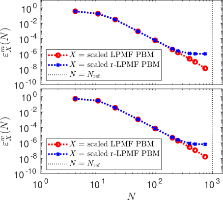
(a) Errors $\varepsilon^{m,w}_{X}(N)$ (61) vs. volume grid size $N$.

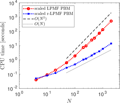
(b) CPU time vs. volume grid size $N$.

Figure 11: 11(a): Relative errors $\varepsilon^{m}_{X},\varepsilon^{w}_{X}$ (61) of the scaled r-LPMF PBM (blue crosses) and LPMF PBM (red circles) with respect to the unscaled LPMF PBM. Computational settings and parameter values are described in detail in Table 4. 11(b): CPU time required for integration of the scaled models in (62) under conditions summarised in Table 4.

	unscaled	scaled	scaled
	LPMF PBMReducing model complexity by means of the Optimal Scaling: Population Balance Model for latex particles morphology formation	LPMF PBMReducing model complexity by means of the Optimal Scaling: Population Balance Model for latex particles morphology formation	r-LPMF PBMReducing model complexity by means of the Optimal Scaling: Population Balance Model for latex particles morphology formation
PBE	(1)-(5)	(1)-(5)	(42)-(45)
ODE	(6)-(13)	(6)-(13)	(46)-(50)
Coefficients $\lambda$	$\lambda=\lambda(\theta,\tilde{p})$ (Table 1), $\tilde{p}=\hat{p}_{\mathrm{exp}}$ (60)
Factors $\theta$	$\theta=\theta_{\mathrm{unit}}=\{\nu_{0},t_{0},d_{0}\}$	$\theta=\tilde{\theta}^{N_{x}}_{\mathrm{opt}}$ (36), $q_{1}=0$
	$\nu_{0}=1\,\mathrm{L}$	$\nu_{0}\approx 4.0\times 10^{-23}\,\mathrm{L}$
	$t_{0}=1\,\mathrm{s}$	$t_{0}\approx 1.5\times 10^{6}\,\mathrm{s}$
	$d_{0}=1\,\mathrm{L}^{-1}$	$d_{0}\approx 4.7\times 10^{45}\,\mathrm{L}^{-1}$
PBE solver	GMOC [9] with (54) and $\sigma_{0}=v_{0}/10$
ODE solver	Runge-Kutta (RK4) [20]
Volume Grid v	$\textbf{v}=\{kh\}_{k=0}^{N}$, $h=V/N$, $V=2v_{0}$
Grid Sizes $N$ and $N_{\mathrm{ref}}$	$N\in 2\mathbb{N}\cap[4,2\times 10^{3}]$, $N_{\mathrm{ref}}=10^{3}$
Time Grid t	$\textbf{t}=\{k\tau\}_{k=0}^{M}$, $\tau=T/M$, $M=10^{3}$
Evaluated time $t=T$	$T=(7.2\times 10^{3}\,\mathrm{s})/t_{0}$
SW/HW	C++ BCAM code, 64-bit Linux OS, 2.40GHz proc.

Table 4: Computational settings and parameter values for integration of the LPMF PBM (1)-(13) and r-LPMF PBM (42)-(50) within the volume domain $[0,V]$ and the time interval $[0,T]$. The symbols $\mathrm{L}$ and $\mathrm{s}$ stand for Litre and second respectively, while $2\mathbb{N}$ labels the set of even natural numbers. Relative errors (61) and computational times are compared in Figure 11. SW/HW stands for Software & Hardware, while BCAM code refers to the in-house package.

Next, we compare numerical solutions of the scaled r-LPMF PBMReducing model complexity by means of the Optimal Scaling: Population Balance Model for latex particles morphology formation and LPMF PBMReducing model complexity by means of the Optimal Scaling: Population Balance Model for latex particles morphology formation obtained with the volume grid size $N$ fixed as specified in Table 5 and the time grid size $M$ increasing up to the reference value $M=M_{\mathrm{ref}}$ reported in Table 5. We take as a reference the solutions of the unscaled LPMF PBMReducing model complexity by means of the Optimal Scaling: Population Balance Model for latex particles morphology formation (see description below (62)) computed with such a time grid size $M=M_{\mathrm{ref}}$. The relative errors between compared solutions are defined as

$$\xi^{y}_{X}(M):=\frac{\max_{v}|y_{X}^{M}(v,T)-y_{Z}^{M_{\mathrm{ref}}}(v,T)|}{\max_{v}|y_{Z}^{M_{\mathrm{ref}}}(v,T)|},\quad Z=\mbox{\footnotesize{unscaled LPMF PBM\ref{foot:1LPMFPBM}}},$$ (63)

where $y_{X}^{M}(v,T)$ denotes the solution $y=m,w$ at volume $v$ and time $t=T$ (see Table 5) of a model $X$ (62) integrated by using a time grid of size $M$. As in (61), the solutions $y_{Z}^{M_{\mathrm{ref}}}(v,T)$ are suitably scaled.

Figure 12 shows relative errors $\xi^{m,w}_{X}(M)$ (63) and computational times required by the scaled LPMF PBMReducing model complexity by means of the Optimal Scaling: Population Balance Model for latex particles morphology formation and r-LPMF PBMReducing model complexity by means of the Optimal Scaling: Population Balance Model for latex particles morphology formation. Table 5 details computational settings and parameter values.

When $M\lesssim 2.5\times 10^{2}$, the relative errors $\xi^{m,w}_{\mbox{\footnotesize{r-LPMF}}}$ are smaller than or equal to $\xi^{m,w}_{\mbox{\footnotesize{LPMF}}}$ (see 12(a)). This means that the scaled r-LPMF PBMReducing model complexity by means of the Optimal Scaling: Population Balance Model for latex particles morphology formation is not only a good approximation of the unscaled LPMF PBMReducing model complexity by means of the Optimal Scaling: Population Balance Model for latex particles morphology formation (for the suggested set of the parameters $\tilde{p}$) but its simplified nature also allows for achieving a better accuracy than it is possible with the scaled LPMF PBMReducing model complexity by means of the Optimal Scaling: Population Balance Model for latex particles morphology formation using the same time/volume grid sizes. Moreover, the computational times required by the scaled r-LPMF PBMReducing model complexity by means of the Optimal Scaling: Population Balance Model for latex particles morphology formation are up to an order of magnitude smaller than the computational times associated with the scaled LPMF PBMReducing model complexity by means of the Optimal Scaling: Population Balance Model for latex particles morphology formation (see 12(b)). For larger values of $M$, i.e. $M\gtrsim 10^{4}$, the difference between the elapsed CPU times is even more pronounced, reaching up to two orders of magnitude. This is because the measured CPU times also account for time spent on writing data to files, whose contribution in the total CPU time decreases (in percentage) with increasing grid sizes.

Finally, we notice that the errors produced by r-LPMF PBMReducing model complexity by means of the Optimal Scaling: Population Balance Model for latex particles morphology formation for $M\gtrsim 10^{3}$ (blue crosses in 12(a)) tend to the same asymptotic value $\approx 10^{-6}$ that was observed in the previous experiments (see 11(a) and Figure 4).

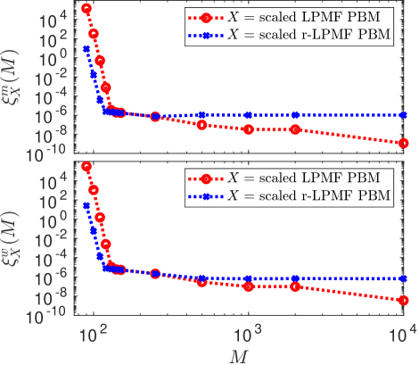
(a) Errors $\xi^{m,w}_{X}(M)$ (63) vs. time grid size $M$.

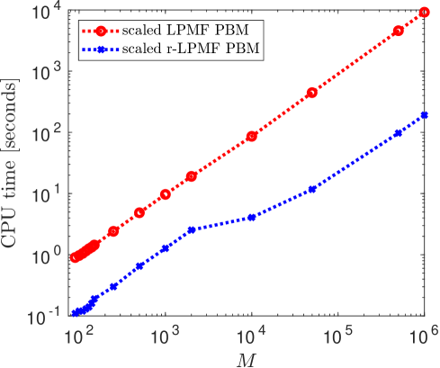
(b) CPU time vs. time grid size $M$.

Figure 12: 12(a): Relative errors $\xi^{m}_{X},\xi^{w}_{X}$ (63) of the scaled r-LPMF PBM (blue crosses) and LPMF PBM (red circles) with respect to the unscaled LPMF PBM. Computational settings and parameter values are described in detail in Table 5. 12(b): CPU time required for integration of the scaled models in (62) under conditions summarised in Table 5.

	unscaled	scaled	scaled
	LPMF PBMReducing model complexity by means of the Optimal Scaling: Population Balance Model for latex particles morphology formation	LPMF PBMReducing model complexity by means of the Optimal Scaling: Population Balance Model for latex particles morphology formation	r-LPMF PBMReducing model complexity by means of the Optimal Scaling: Population Balance Model for latex particles morphology formationReducing model complexity by means of the Optimal Scaling: Population Balance Model for latex particles morphology formation
PBE	(1)-(5)	(1)-(5)	(42)-(45)
ODE	(6)-(13)	(6)-(13)	(46)-(50)
Coefficients $\lambda$	$\lambda=\lambda(\theta,\tilde{p})$ (Table 1), $\tilde{p}=\hat{p}_{\mathrm{exp}}$ (60)
Factors $\theta$	$\theta=\theta_{\mathrm{unit}}=\{\nu_{0},t_{0},d_{0}\}$	$\theta=\tilde{\theta}^{N_{x}}_{\mathrm{opt}}$ (36), $q_{1}=0$
	$\nu_{0}=1\,\mathrm{L}$	$\nu_{0}\approx 4.0\times 10^{-23}\,\mathrm{L}$
	$t_{0}=1\,\mathrm{s}$	$t_{0}\approx 1.5\times 10^{6}\,\mathrm{s}$
	$d_{0}=1\,\mathrm{L}^{-1}$	$d_{0}\approx 4.7\times 10^{45}\,\mathrm{L}^{-1}$
PBE solver	GMOC [9] with (54) and $\sigma_{0}=v_{0}/10$
ODE solver	Runge-Kutta (RK4) [20]
Volume Grid v	$\textbf{v}=\{kh\}_{k=0}^{N}$, $h=V/N$, $V=2v_{0}$, $N=250$
Time Grid t	$\textbf{t}=\{k\tau\}_{k=0}^{M}$, $\tau=T/M$
Grid Sizes $M$ and $M_{\mathrm{ref}}$	$M\in[90,10^{6}]$, $M_{\mathrm{ref}}=10^{6}$
Evaluated time $t=T$	$T=(7.2\times 10^{3}\,\mathrm{s})/t_{0}$
SW/HW	C++ BCAM code, 64-bit Linux OS, 2.40GHz proc.

Table 5: Computational settings and parameter values for integration of the LPMF PBM (1)-(13) and r-LPMF PBM (42)-(50) within the volume domain $[0,V]$ and the time interval $[0,T]$. The symbols $\mathrm{L}$ and $\mathrm{s}$ stand for Litre and second respectively. Relative errors (63) and computational times are compared in Figure 12. SW/HW stands for Software & Hardware, while BCAM code refers to the in-house package.

6 Conclusions

In this paper, we explore the feasibility of the reduction of complexity of the Population Balance Model for Latex Particles Morphology Formation, LPMF PBMReducing model complexity by means of the Optimal Scaling: Population Balance Model for latex particles morphology formation, through disregard of the aggregation terms of the model. The recent nondimensionalization procedure Optimal Scaling (OS) [9] is employed under the mathematically supported constraints to reveal a quantitative criterion for locating regions of slow and fast aggregation. Such a criterion helps to recognize those physical parameters that suppress aggregation and enable the use of dimensionless population models of reduced complexity, denoted as r-LPMF PBMReducing model complexity by means of the Optimal Scaling: Population Balance Model for latex particles morphology formation in this work. The models are derived by means of the OSReducing model complexity by means of the Optimal Scaling: Population Balance Model for latex particles morphology formation with constraints (OSC) and are mathematically justified.

In comparison with the LPMF PBMReducing model complexity by means of the Optimal Scaling: Population Balance Model for latex particles morphology formation, the new models are lacking integral terms, and all their solely time-dependent components are computed without resorting to preceding or successive solutions of the governing population balance equations. These features result in improved computational performance and also open the opportunity to facilitate numerical integration algorithms for solving effectively the proposed models.

Comparative performance of the r-LPMF PBMReducing model complexity by means of the Optimal Scaling: Population Balance Model for latex particles morphology formation and LPMF PBMReducing model complexity by means of the Optimal Scaling: Population Balance Model for latex particles morphology formation with the physically validated parameters values [7] is investigated. The numerical tests reveal that in order to maintain the same level of accuracy, the r-LPMF PBMReducing model complexity by means of the Optimal Scaling: Population Balance Model for latex particles morphology formation requires up to 2 orders of magnitude less computational effort than it is needed by the LPMF PBMReducing model complexity by means of the Optimal Scaling: Population Balance Model for latex particles morphology formation.

The results presented in this paper can be beneficial to particle aggregation studies, e.g., [21, 22], investigating slow and fast aggregation regimes, as well as estimating the corresponding rate constants. In particular, our scaling procedure allows determining an upper bound for rates leading to slow aggregation. Under such a regime, the reduced complexity of the r-LPMF PBMReducing model complexity by means of the Optimal Scaling: Population Balance Model for latex particles morphology formation permits a more accessible insight into the system’s properties. In this light, our future direction is to explore the possibilities for enhancing the numerical treatment of the introduced r-LPMF PBMReducing model complexity by means of the Optimal Scaling: Population Balance Model for latex particles morphology formation, taking full advantages of its simplified structure, in order to enable on-the-fly recommendations for technological conditions in the synthesis of new multiphase morphologies.

Appendix A LPMF PBM: Time-Dependent Factors of Rate Functions

Here, we characterise the dependency on time of rate functions $\alpha(v,u,t)$ (2), $g(v,t)$ (3) and $n(v,t)$ (4). In particular, we focus on their time-dependent factors

$$\tilde{\textbf{p}}(t):=\{\tilde{\alpha}_{0}(t),\tilde{\varrho}_{\mathrm{d}}(t),\tilde{\varrho}_{\mathrm{p}}(t),\tilde{\eta}_{0}(t)\},\quad\forall t\in\mathbb{R}^{+}.$$ (A.1)

As shown in Section 2, the factors $\tilde{\textbf{p}}(t)$ depend on $\Psi(t)$ (9), $\Phi(t)$ (11) and $V_{p}(t)$ (12). First, it is possible to show that

$$\Psi(t)\in(0,\bar{\Psi}],\quad\forall t\in\mathbb{R}^{+},\quad\mbox{and}\quad\lim_{t\to\infty}\Psi(t)=0.$$ (A.2)

Let us denote

$$z(t):=\Psi(t)\,e^{\int_{0}^{t}\!F(s)\,ds},\quad\mbox{with}\quad F(t):=\frac{\lambda_{\mathrm{p}}\,(\Psi(t)+\Psi_{r})}{(\Psi(t)+1)(V_{\mathrm{pol2}}(t)+\lambda_{\mathrm{pol1}})},\quad\forall t\in\mathbb{R}^{+},$$ (A.3)

where $\Psi(t)$ is a solution of the ODE (9). We observe that $z^{\prime}(t)=0$ and $z(t)=z(0)=\Psi(0)=\bar{\Psi}$, $\forall t\in\mathbb{R}^{+}$. By using the above definition of $z(t)$, one obtains an implicit relation for $\Psi(t)$:

$$\Psi(t)=\bar{\Psi}\,e^{-\int_{0}^{t}\!F(s)\,ds},\quad\forall t\in\mathbb{R}^{+}.$$ (A.4)

Then, (A.4) implies that $\Psi(t)>0$, $\forall t\in\mathbb{R}^{+}$. From (10), $V_{\mathrm{pol2}}(0)=0$ and $V^{\prime}_{\mathrm{pol2}}(t)>0$, $\forall t\in\mathbb{R}^{+}$. Thus, $V_{\mathrm{pol2}}(t)\geq 0$ and $F(t)>0$, $\forall t\in\mathbb{R}^{+}$. Then, $\Psi(t)\leq\bar{\Psi}$, $V^{\prime}_{\mathrm{pol2}}(t)<\lambda_{\mathrm{p}}\,\bar{\Psi}$, $V_{\mathrm{pol2}}(t)<\lambda_{\mathrm{p}}\,\bar{\Psi}\,t$ and $F(t)>(\lambda_{\mathrm{p}}\,\Psi_{r})/[(\bar{\Psi}+1)(\lambda_{\mathrm{p}}\,\bar{\Psi}\,t+\lambda_{\mathrm{pol1}})]$, $\forall t\in\mathbb{R}^{+}$. As a consequence, $\int_{0}^{t}\!F(s)\,ds$ diverges to $\infty$, $\Psi(t)$ (A.4) tends to $0$, as $t\to\infty$, and thus (A.2) follows.

Then, we show that

$$V_{p}(t)>\lambda_{\mathrm{pol1}}>0,\quad\forall t\in\mathbb{R}^{+}.$$ (A.5)

By summing (6), (7) and (8), one obtains (10). In other words, one has

$$\begin{cases}\frac{dV^{\mathrm{mat}}_{\mathrm{pol2}}(t)}{dt}+\frac{dV^{\mathrm{c_{m}}}_{\mathrm{pol2}}(t)}{dt}+\frac{dV^{\mathrm{c_{w}}}_{\mathrm{pol2}}(t)}{dt}&=\frac{dV_{\mathrm{pol2}}(t)}{dt},\quad\forall t\in\mathbb{R}^{+},\\ V^{\mathrm{mat}}_{\mathrm{pol2}}(0)+V^{\mathrm{c_{m}}}_{\mathrm{pol2}}(0)+V^{\mathrm{c_{w}}}_{\mathrm{pol2}}(0)&=V_{\mathrm{pol2}}(0).\end{cases}$$ (A.6)

By integrating (A.6) over $[0,t]$, it follows

$$V^{\mathrm{mat}}_{\mathrm{pol2}}(t)+V^{\mathrm{c_{m}}}_{\mathrm{pol2}}(t)+V^{\mathrm{c_{w}}}_{\mathrm{pol2}}(t)=V_{\mathrm{pol2}}(t),\quad\forall t\in\mathbb{R}^{+}.$$ (A.7)

By plugging (A.7) in (12), one obtains

$$V_{p}(t)=\,\left(\Psi(t)+1\right)\,\left[V_{\mathrm{pol2}}(t)+\lambda_{\mathrm{pol1}}\right]>\lambda_{\mathrm{pol1}}>0,\quad\forall t\in\mathbb{R}^{+}.$$ (A.8)

that concludes a proof of (A.5).

Finally, we demonstrate that

$$\Phi(t)\in[0,1),\quad\forall t\in\mathbb{R}^{+}.$$ (A.9)

Definition (11) implies that $\Phi(t)$ is non-negative for any $t\in\mathbb{R}^{+}$ and $\Phi(0)=0$. Then, (6) shows that $dV^{\mathrm{mat}}_{\mathrm{pol2}}(t)/dt>0$ when $V^{\mathrm{mat}}_{\mathrm{pol2}}(t)=0$. Thus, $V^{\mathrm{mat}}_{\mathrm{pol2}}(t)\geq 0$, $\forall t\in\mathbb{R}^{+}$. As a consequence

$$\Phi(t)\leq\frac{V^{\mathrm{mat}}_{\mathrm{pol2}}(t)}{(\Psi(t)+1)(V^{\mathrm{mat}}_{\mathrm{pol2}}(t)+\lambda_{\mathrm{pol1}})}<1,\quad\forall t\in\mathbb{R}^{+}.$$ (A.10)

In conclusion, (A.2), (A.5) and (A.9) provide insight into properties of the time-dependent factors $\tilde{\textbf{p}}(t)$, as summarised in Table A.1. In the following Appendices we prove the important properties of the LPMF PBMReducing model complexity by means of the Optimal Scaling: Population Balance Model for latex particles morphology formation which make its approximation with the r-LPMF PBMReducing model complexity by means of the Optimal Scaling: Population Balance Model for latex particles morphology formation possible.

Sign	Admits Zero-Value
$\tilde{\alpha}_{0}(t)>0$, $\forall t\in\mathbb{R}^{+}$	No: $\tilde{\alpha}_{0}(t)>\lambda_{\mathrm{a}}>0$, $\forall t\in\mathbb{R}^{+}$
$\tilde{\varrho}_{\mathrm{d}}(t)\geq 0$, $\forall t\in\mathbb{R}^{+}$	Yes: $\tilde{\varrho}_{\mathrm{d}}(t)=0\Leftrightarrow\Phi(t)=0$, e.g. $t=0$
$\tilde{\varrho}_{\mathrm{p}}(t)>0$, $\forall t\in\mathbb{R}^{+}$	No, but $\lim_{t\to\infty}\tilde{\varrho}_{\mathrm{p}}(t)=0$
$\tilde{\eta}_{0}(t)\geq 0$, $\forall t\in\mathbb{R}^{+}$	Yes: $\tilde{\eta}_{0}(t)=0\Leftrightarrow\Phi(t)=0$, e.g. $t=0$
Upper Bound
$\tilde{\alpha}_{0}(t)\leq\kappa_{\mathrm{a}}:=\lambda_{\mathrm{a}}\,(\bar{\Psi}+1)^{\nicefrac{{14}}{{3}}}<\infty$, $\forall t\in\mathbb{R}^{+}$
$\tilde{\varrho}_{\mathrm{d}}(t)<\kappa_{\mathrm{d}}:=\lambda_{\mathrm{d}}\,(\bar{\Psi}+1)^{\nicefrac{{2}}{{3}}}<\infty$, $\forall t\in\mathbb{R}^{+}$
$\tilde{\varrho}_{\mathrm{p}}(t)<\kappa_{\mathrm{p}}:=\lambda_{\mathrm{p}}\,\bar{\Psi}/\lambda_{\mathrm{pol1}}<\infty$, $\forall t\in\mathbb{R}^{+}$
$\tilde{\eta}_{0}(t)<\kappa_{\mathrm{n}}:=\lambda_{\mathrm{n}}<\infty$, $\forall t\in\mathbb{R}^{+}$

Table A.1: Properties of factors $\tilde{\textbf{p}}(t)=\{\tilde{\alpha}_{0}(t),\tilde{\varrho}_{\mathrm{d}}(t),\tilde{\varrho}_{\mathrm{p}}(t),\tilde{\eta}_{0}(t)\}$ of rate functions (2)-(4). The table provides the sign of factors $\tilde{\textbf{p}}$, whenever they admit zero as a possible value and the upper bounds on their time-evolution. We remark that the coefficients $\lambda_{\mathrm{a}},\lambda_{\mathrm{d}}$ in (2)-(3) depend on the parameters $a,b$ (see Table 1), however, all the summarised here properties hold for any finite value of $a,b\in\mathbb{R}$ and $\bar{\Psi}>0$.

Appendix B LPMF PBM: Solutions in $B_{0}:=\{(v,t)\in[0,\infty)^{2}:\,v<v_{0},\,v_{0}>0\}$

Proposition B.1.

If $a\in\mathbb{R}$, $0<b<1$, $v_{0}>0$ and $m(v,t)$, $w(v,t)$ are the solutions to (1)-(13), then $m(v,t)=w(v,t)=0$, $\forall v\in[0,v_{0})$, $\forall t\in\mathbb{R}^{+}$.

Proof.

We provide the proof for $m(v,t)$ only, but the same argument applies to $w(v,t)$.

Let us define $M^{x}_{v}(t):=\int_{0}^{v}\!u^{x}\,m(u,t)\,du$ for all $v,t\in\mathbb{R}^{+}$ and $x\in\mathbb{R}$. Then, for $v\in(0,v_{0})$, $a\in\mathbb{R}$ and $0<b<1$, the evolution equation of $M^{0}_{v}(t)$ reads:

$$\begin{cases}\frac{d}{dt}M^{0}_{v}(t)&=-g(v,t)m(v,t)-\mu\,M^{0}_{v}(t)-\tilde{\alpha}_{0}(t)M^{a}_{v}(t)M^{0}_{\infty}(t)-\tilde{\alpha}_{0}(t)M^{0}_{v}(t)M^{a}_{\infty}(t)+\\ &\quad+\frac{\tilde{\alpha}_{0}(t)}{2}\,\int_{0}^{v}\!m(u,t)\,\int_{0}^{v-u}[y^{a}+u^{a}]\,m(y,t)\,dy\,du,\quad\forall v\in(0,v_{0}),\,\forall t\in\mathbb{R}^{+},\\ M^{0}_{v}(0)&=0,\quad\forall v\in(0,v_{0}),\end{cases}$$ (B.1)

with $\mu=\lambda_{\mathrm{m}}>0$ (see Table 1) and $g$ given by (3), such that $g(v,t)\geq 0$, $\forall v,t\in\mathbb{R}^{+}$ (see Table A.1). Since $\tilde{\alpha}_{0}(t)$ and $m(v,t)$ are non-negative for all $v,t\in\mathbb{R}^{+}$, as shown in Appendix A and [9], we have

$$\tilde{\alpha}_{0}(t)M^{a}_{v}(t)M^{0}_{\infty}(t)+\tilde{\alpha}_{0}(t)M^{0}_{v}(t)M^{a}_{\infty}(t)\geq 2\tilde{\alpha}_{0}(t)M^{a}_{v}(t)M^{0}_{v}(t),$$ (B.2)

and

$$\frac{\tilde{\alpha}_{0}(t)}{2}\,\int_{0}^{v}\!m(u,t)\,\int_{0}^{v-u}[y^{a}+u^{a}]\,m(y,t)\,dy\,du\leq\tilde{\alpha}_{0}(t)M^{a}_{v}(t)M^{0}_{v}(t).$$ (B.3)

Then from (B.1)-(B.3) and $0\leq M^{a}_{v}(t)M^{0}_{v}(t)\leq\infty$, it follows $dM^{0}_{v}(t)/dt\leq 0$ and $M^{0}_{v}(t)\leq M^{0}_{v}(0)=0$, $\forall v\in(0,v_{0})$, $\forall t\in\mathbb{R}^{+}$. Since $M^{0}_{v}(t)$ must be non-negative, we conclude that $M^{0}_{v}(t)=0$, $\forall v\in(0,v_{0})$, $\forall t\in\mathbb{R}^{+}$.

Finally, one has:

$$m(v,t)=\frac{d}{dv}\int_{0}^{v}\!m(u,t)\,du=\frac{d}{dv}M^{0}_{v}(t)=0,\quad\forall v\in(0,v_{0}),\,\forall t\in\mathbb{R}^{+},$$ (B.4)

and Proposition B.1 follows (rem. $m(0,t)=0$, $\forall t\in\mathbb{R}^{+}$). ∎

Appendix C LPMF PBM: Finiteness of Distributions Moments

Proposition C.1.

Given $a\in\mathbb{R}$, $0<b<1$ and $v_{0}>0$, the moments $M^{0}(t):=\int_{0}^{\infty}\!m(v,t)\,dv$ and $W^{0}(t):=\int_{0}^{\infty}\!w(v,t)\,dv$ of solutions to (1)-(13) are finite for all times $t\in\mathbb{R}^{+}$ and $M^{0}(t)\leq\kappa_{\mathrm{n}}\,t$, $W^{0}(t)\leq\frac{\kappa_{\mathrm{n}}\,\lambda_{\mathrm{m}}}{2}\,t^{2}$, $\forall t\in\mathbb{R}^{+}$. Here, $\kappa_{\mathrm{n}}\in(0,\infty)$ is the upper bound of the factor $\tilde{\eta}_{0}(t)$ provided in Table A.1 and $\lambda_{\mathrm{m}}\in(0,\infty)$ is defined in Table 1.

Proof.

When $a\in\mathbb{R}$, $0<b<1$ and $v_{0}>0$, the evolution equations for the moments $M^{0}(t)$ and $W^{0}(t)$, $\forall t\in\mathbb{R}^{+}$, are given by

$$\begin{cases}\frac{dM^{0}(t)}{dt}&=-\lim_{v\to\infty}g^{0}_{m}(v,t)+\tilde{\eta}_{0}(t)-\mu\,M^{0}(t)-\tilde{\alpha}_{0}(t)\left[2M^{a}(t)M^{0}(t)-M^{a}(t)M^{0}(t)\right],\\ \frac{dW^{0}(t)}{dt}&=-\lim_{v\to\infty}g^{0}_{w}(v,t)+\mu\,M^{0}(t)-\tilde{\alpha}_{0}(t)\left[2W^{a}(t)W^{0}(t)-W^{a}(t)W^{0}(t)\right],\\ M^{0}(0)&=W^{0}(0)=0,\end{cases}$$ (C.1)

with

$$g^{x}_{y}(v,t):=(\tilde{\varrho}_{\mathrm{d}}(t)v^{x+b}+\tilde{\varrho}_{\mathrm{p}}(t)v^{x+1})\,y(v,t)\geq 0,\quad y=m,w,\quad\forall x\in\mathbb{R},\quad\forall v,t\in\mathbb{R}^{+}.$$ (C.2)

For any $t\in\mathbb{R}^{+}$ such that $0\leq M^{a}(t)M^{0}(t)\leq\infty$ and $0\leq W^{a}(t)W^{0}(t)\leq\infty$, we can assure that $2M^{a}(t)M^{0}(t)\geq M^{a}(t)M^{0}(t)$ and $2W^{a}(t)W^{0}(t)\geq W^{a}(t)W^{0}(t)$. Since $\tilde{\alpha}_{0}(t),m(v,t)$ and $w(v,t)$ are non-negative for all $v,t\in\mathbb{R}^{+}$, as shown in Appendix A and [9], it follows

$$\frac{dM^{0}(t)}{dt}\leq\kappa_{\mathrm{n}},\quad\frac{dW^{0}(t)}{dt}\leq\lambda_{\mathrm{m}}\,M^{0}(t),\quad\forall t\in\mathbb{R}^{+},$$ (C.3)

with $\kappa_{\mathrm{n}}\in(0,\infty)$ being the upper bound of the factor $\tilde{\eta}_{0}(t)$ provided in Table A.1 and $\mu=\lambda_{\mathrm{m}}\in(0,\infty)$ (5). Integrating (C.3) over $[0,t]$ and using the initial conditions in (C.1), we get the bounds of $M^{0}(t)$, $W^{0}(t)$ stated in Proposition C.1 and this concludes the proof. ∎

Proposition C.2.

Given $a\leq 0$, $0<b<1$, $v_{0}>0$ and any finite $x,y\in\mathbb{R}$ such that $x\leq y$, there exist strictly positive quantities $K^{x}_{m},K^{x}_{w}<\infty$, dependent on the chosen $x$, but independent of time $t$, such that the moments $M^{x}(t):=\int_{0}^{\infty}\!v^{x}\,m(v,t)\,dv$ and $W^{x}(t):=\int_{0}^{\infty}\!v^{x}\,w(v,t)\,dv$ of solutions to (1)-(13) satisfy $M^{x}(t)\leq K^{x}_{m}+M^{y}(t)$, $W^{x}(t)\leq K^{x}_{w}+W^{y}(t)$, $\forall t\in[0,T]$, with any fixed $T<\infty$.

Proof.

We obtain an upper bound on $M^{x}(t)$ only, as similar estimates can be made for $W^{x}(t)$.

Proposition B.1 implies that $M^{x}(t)=\int_{v_{0}}^{\infty}\!v^{x}\,m(v,t)\,dv$, $\forall x\in\mathbb{R}$, $\forall t\in\mathbb{R}^{+}$. Then, if $\bar{v}\in\mathbb{R}$ is chosen such that $\max\{v_{0},1\}<\bar{v}<\infty$, it follows ($\forall x\in\mathbb{R}$)

$$M^{x}(t)=\int_{v_{0}}^{\bar{v}}\!v^{x}\,m(v,t)\,dv+\int_{\bar{v}}^{\infty}\!v^{x}\,m(v,t)\,dv,\quad\forall t\in\mathbb{R}^{+},\quad\mbox{with}\quad\max\{v_{0},1\}<\bar{v}<\infty.$$ (C.4)

Fixing $\bar{v}$ as above, we have $\int_{v_{0}}^{\bar{v}}\!v^{x}\,m(v,t)\,dv\leq c_{x}\,S_{m}(t)$, $\forall t\in\mathbb{R}^{+}$, where $c_{x}:=\int_{v_{0}}^{\bar{v}}\!v^{x}\,dv$, $0<c_{x}<\infty$, $\forall x\in\mathbb{R}$, and $S_{m}(t):=\sup_{v\in\mathbb{R}^{+}}|m(v,t)|$, $\forall t\in\mathbb{R}^{+}$.

We also notice that $v^{x}\leq v^{y}$, $\forall x\leq y\in\mathbb{R}$, whenever $v>1$. Indeed, the function $f:\mathbb{R}\to\mathbb{R}^{+}$, $f(x):=v^{x}$, is increasing with respect to its argument $x\in\mathbb{R}$ if $v>1$. Then, provided $m(v,t)$ to be non-negative (as shown in [9]) and $\bar{v}>1$, one has

$$\int_{\bar{v}}^{\infty}\!v^{x}\,m(v,t)\,dv\leq\int_{\bar{v}}^{\infty}\!v^{y}\,m(v,t)\,dv\leq M^{y}(t),\quad\forall x\leq y\in\mathbb{R},\quad\forall t\in\mathbb{R}^{+}.$$ (C.5)

By using the derived above inequalities, one obtains the statement of Proposition C.2:

$$M^{x}(t)\leq c_{x}\,S_{m}(t)+M^{y}(t)\leq K^{x}_{m}+M^{y}(t),\quad\forall x\leq y\in\mathbb{R},\quad\forall t\in[0,T],$$ (C.6)

where $T<\infty$ and, thus, the estimate (D.25) for $S_{m}(t)$ (D.21) can be used (together with $c_{x}$ given above) to obtain the quantity $0<K^{x}_{m}<\infty$ dependent on $x$, i.e. on $c_{x}$, but independent of time $t$. ∎

Proposition C.3.

Given $a\leq 0$, $0<b<1$, $v_{0}>0$, the moments $M^{1}(t):=\int_{0}^{\infty}\!v\,m(v,t)\,dv$ and $W^{1}(t):=\int_{0}^{\infty}\!v\,w(v,t)\,dv$ of solutions to (1)-(13) are finite for all times $t\in\mathbb{R}^{+}$.

Proof.

If $a\leq 0$, $0<b<1$, $v_{0}>0$, the evolution equations for $M^{1}(t)$ and $W^{1}(t)$ read, $\forall t\in\mathbb{R}^{+}$,

$$\begin{cases}\frac{dM^{1}(t)}{dt}&=-\,\lim_{v\to\infty}\,g^{1}_{m}(v,t)\,+\,(\tilde{\varrho}_{\mathrm{p}}(t)-\mu)\,M^{1}(t)\,+\,\tilde{\varrho}_{\mathrm{d}}(t)\,M^{b}(t)\,+\,\tilde{\eta}_{0}(t)\,v_{0}\,-\\ &\quad-\,\tilde{\alpha}_{0}(t)\,\left[\,M^{1+a}(t)\,M^{0}(t)\,+\,M^{1}(t)\,M^{a}(t)\,\,-\,\,M^{1+a}(t)\,M^{0}(t)\,-\,M^{1}(t)\,M^{a}(t)\,\right],\\ \frac{dW^{1}(t)}{dt}&=-\,\lim_{v\to\infty}\,g^{1}_{w}(v,t)\,+\,\tilde{\varrho}_{\mathrm{p}}(t)\,W^{1}(t)\,+\,\tilde{\varrho}_{\mathrm{d}}(t)\,W^{b}(t)\,+\,\mu\,M^{1}(t)\,-\\ &\quad-\,\tilde{\alpha}_{0}(t)\,\left[\,W^{1+a}(t)\,W^{0}(t)\,+\,W^{1}(t)\,W^{a}(t)\,\,-\,\,W^{1+a}(t)\,W^{0}(t)\,-\,W^{1}(t)\,W^{a}(t)\,\right],\\ M^{1}(0)&=W^{1}(0)=0,\end{cases}$$ (C.7)

with $g^{x}_{m},g^{x}_{w}$ given as (C.2), $M^{x}(t):=\int_{0}^{\infty}\!v^{x}\,m(v,t)\,dv$ and $W^{x}(t):=\int_{0}^{\infty}\!v^{x}\,w(v,t)\,dv$, $\forall x\in\mathbb{R}$.

Using the non-negativity of $g^{1}_{m},g^{1}_{w}$ (C.2), $\mu$ (5), $m(v,t)$ and $w(v,t)$ [9], together with the bounds provided in Table A.1, one obtains $\forall t\in\mathbb{R}^{+}$

$$\begin{cases}\frac{dM^{1}(t)}{dt}&\leq\kappa_{\mathrm{p}}\,M^{1}(t)\,+\,\kappa_{\mathrm{d}}\,M^{b}(t)\,+\,\kappa_{\mathrm{n}}\,v_{0}\,+\,\kappa_{\mathrm{a}}\,\left[\,M^{1+a}(t)\,M^{0}(t)\,+\,M^{1}(t)\,M^{a}(t)\,\right],\\ \frac{dW^{1}(t)}{dt}&\leq\kappa_{\mathrm{p}}\,W^{1}(t)\,+\,\kappa_{\mathrm{d}}\,W^{b}(t)\,+\,\mu\,M^{1}(t)\,+\,\kappa_{\mathrm{a}}\,\left[\,W^{1+a}(t)\,W^{0}(t)\,+\,W^{1}(t)\,W^{a}(t)\,\right],\\ M^{1}(0)&=W^{1}(0)=0.\end{cases}$$ (C.8)

When time $t$ belongs to the finite interval $[0,T]$, with any fixed $T<\infty$, Proposition C.2 allows us writing (note that $a\leq 0$, $0<b<1$ and $v_{0}>0$)

$$\begin{cases}\frac{dM^{1}(t)}{dt}&\leq\kappa_{\mathrm{p}}\,M^{1}(t)\,+\,\kappa_{\mathrm{d}}\,(K^{b}_{m}+M^{1}(t))\,+\,\kappa_{\mathrm{n}}\,v_{0}\,+\\ &\quad+\,\kappa_{\mathrm{a}}\left[\,M^{0}(t)\,(K^{1+a}_{m}+M^{1}(t))\,+\,(K^{a}_{m}+M^{0}(t))\,M^{1}(t)\,\right],\quad\forall t\in[0,T],\\ \frac{dW^{1}(t)}{dt}&\leq\kappa_{\mathrm{p}}\,W^{1}(t)\,+\,\kappa_{\mathrm{d}}\,(K^{b}_{w}+W^{1}(t))\,+\,\mu\,M^{1}(t)\,+\\ &\quad+\,\kappa_{\mathrm{a}}\,\left[\,W^{0}(t)\,(K^{1+a}_{w}+W^{1}(t))\,+\,(K^{a}_{w}+W^{0}(t))\,W^{1}(t)\,\right],\quad\forall t\in[0,T],\\ M^{1}(0)&=W^{1}(0)=0,\end{cases}$$ (C.9)

with $0<K^{x}_{m},K^{x}_{w}<\infty$, $\forall x\in\mathbb{R}$, independent of time $t$. Moreover, Proposition C.1 holds for $M^{0}(t)$ and $W^{0}(t)$ (i.e. $M^{0}(t)\leq\kappa_{\mathrm{n}}\,t$, $W^{0}(t)\leq\frac{\kappa_{\mathrm{n}}\,\lambda_{\mathrm{m}}}{2}\,t^{2}$, $\forall t\in\mathbb{R}^{+}$) providing

$$\begin{cases}\frac{dM^{1}(t)}{dt}&\leq\kappa_{\mathrm{p}}\,M^{1}(t)\,+\,\kappa_{\mathrm{d}}\,(K^{b}_{m}+M^{1}(t))\,+\,\kappa_{\mathrm{n}}\,v_{0}\,+\\ &\quad+\,\kappa_{\mathrm{a}}\left[\,\kappa_{\mathrm{n}}\,t\,(K^{1+a}_{m}+M^{1}(t))\,+\,(K^{a}_{m}+\kappa_{\mathrm{n}}t)\,M^{1}(t)\,\right],\quad\forall t\in[0,T],\\ \frac{dW^{1}(t)}{dt}&\leq\kappa_{\mathrm{p}}\,W^{1}(t)\,+\,\kappa_{\mathrm{d}}\,(K^{b}_{w}+W^{1}(t))\,+\,\mu\,M^{1}(t)\,+\\ &\quad+\,\kappa_{\mathrm{a}}\,\left[\,\frac{\kappa_{\mathrm{n}}\,\lambda_{\mathrm{m}}}{2}\,t^{2}\,(K^{1+a}_{w}+W^{1}(t))\,+\,(K^{a}_{w}+\frac{\kappa_{\mathrm{n}}\,\lambda_{\mathrm{m}}}{2}\,t^{2})\,W^{1}(t)\,\right],\quad\forall t\in[0,T],\\ M^{1}(0)&=W^{1}(0)=0.\end{cases}$$ (C.10)

In the case of $M^{1}(t)$, one obtains by integrating (C.10) over $[0,t]$, with $t\in[0,T]$, $T<\infty$:

$$M^{1}(t)\leq h(t)+\int_{0}^{t}\!k(s)\,M^{1}(s)\,ds,\quad\forall t\in[0,T],\quad T<\infty,$$ (C.11)

with $h(t):=k_{1}\,t+k_{2}\,t^{2}$, $k(t):=k_{3}+k_{4}\,t$ and $0<k_{i}<\infty$ independent of time $t$, $\forall i=1,\dots,4$. Indeed, such quantities $k_{i}$, $\forall i=1,\dots,4$, depend only on the time-independent constants in (C.10). Since $h(t)$ and $k(t)$ are continuous, non-negative and non-decreasing functions on $[0,T]$, a Gronwall’s inequality (Theorem A in [23]) leads to

$$M^{1}(t)\leq h(t)\,e^{\int_{0}^{t}\!k(\xi)\,d\xi}\leq(k_{1}T+k_{2}T^{2})\,e^{k_{3}T+k_{4}T^{2}}<\infty,\quad\forall t\in[0,T],\quad T<\infty.$$ (C.12)

As $T$ can be arbitrarily chosen in $(0,\infty)$, (C.12) implies $M^{1}(t)<\infty$, $\forall t\in\mathbb{R}^{+}$.

To prove finiteness of $W^{1}(t)$, $\forall t\in\mathbb{R}^{+}$, we first notice that (C.12) along with $0<\mu=\lambda_{\mathrm{m}}<\infty$ (Table 1) confirm the finiteness of the term $\mu\,M^{1}(t)$ in the second inequality in (C.10). Then, it is possible to invoke a Gronwall’s inequality for $W^{1}(t)$ similar to the discussed for $M^{1}(t)$ and, thus, to conclude the proof. ∎

Appendix D LPMF PBM: Boundedness of Solutions

Proposition D.1.

Given $a\leq 0$, $0<b<1$ and $v_{0}>0$, the solutions $m(v,t)$ and $w(v,t)$ to (1)-(13) are bounded for $v\in\mathbb{R}^{+}$ and $t\in[0,T]$, with any fixed $T<\infty$.

Proof.

We provide a proof for $m(v,t)$ only, as similar arguments apply to $w(v,t)$. We start by denoting

$$\tilde{g}(v,t):=\begin{cases}g(v,t),&\mathrm{for}\quad v\geq v_{0},\,t\in\mathbb{R}^{+},\\ g(v_{0},t),&\mathrm{for}\quad v<v_{0},\,t\in\mathbb{R}^{+},\end{cases}$$ (D.1)

and

$$\tilde{\alpha}(v,u,t):=\begin{cases}\alpha(v,u,t),&\mathrm{if}\quad v,u\geq v_{0},\,t\in\mathbb{R}^{+},\\ \alpha(v_{0},v_{0},t),&\mathrm{otherwise},\end{cases}$$ (D.2)

where $g(v,t)=\tilde{\varrho}_{\mathrm{d}}(t)\,v^{b}+\tilde{\varrho}_{\mathrm{p}}(t)\,v$ (3), $v_{0}>0$, $\alpha(v,u,t)=\tilde{\alpha}_{0}(t)[v^{a}+u^{a}]$ (2) and $a\leq 0$. We consider now (1) but with $\tilde{g}$ and $\tilde{\alpha}$ instead of $g$ and $\alpha$ respectively:

$$\partial_{t}m(v,t)\,+\,\tilde{g}(v,t)\,\partial_{v}m(v,t)\,+\,\partial_{v}\tilde{g}(v,t)\,m(v,t)\,+\,\mu\,m(v,t)=\tilde{\eta}_{0}(t)\,\delta(v-v_{0})\,+\,\mathcal{I}_{m}(v,t).$$ (D.3)

Here

$$\mathcal{I}_{m}(v,t):= \,\frac{1}{2}\,\int_{-\infty}^{\infty}\!\tilde{\alpha}(v-u,u,t)\,m(v-u,t)\,m(u,t)\,du\,-$$

$$-\,m(v,t)\,\int_{-\infty}^{\infty}\!\tilde{\alpha}(v,u,t)\,m(u,t)\,du$$ (D.4)

and $m(v,t)$ has been set to $0$ for all $v<0$ and $t\in\mathbb{R}^{+}$. We shall continue reasoning just for (D.3) and at the end, taking into account that Proposition B.1 still holds for this equation (as well as for (1)) and $\tilde{g}\equiv g$, $\tilde{\alpha}\equiv\alpha$ for $v,u\geq v_{0}$, our derivation will also hold for (1).

We denote by $\varphi(t,v_{*})$ the solution at time $t$, with initial data $v_{*}\in\mathbb{R}$, of the ODE:

$$\begin{cases}\frac{d}{dt}\varphi(t,v_{*})&=\tilde{g}(\varphi(t,v_{*}),t),\quad\forall t\in\mathbb{R}^{+},\\ \varphi(0,v_{*})&=v_{*}.\end{cases}$$ (D.5)

The ODE provides a well-defined solution and a global flow $v=\varphi(t,v_{*})$ and its inverse (in the second variable) $v_{*}=\varphi_{*}(t,v)$ as long as $\tilde{g}$ is Lipschitz (has bounded derivatives) in its variable $v$ (see [24], pp. $129-130$). Indeed,

$$\partial_{v}\tilde{g}(v,t)=\begin{cases}\tilde{\varrho}_{\mathrm{d}}(t)\,b\,v^{b-1}\,+\,\tilde{\varrho}_{\mathrm{p}}(t),&\mathrm{for}\quad v\geq v_{0},\\ 0&\mathrm{for}\quad v<v_{0},\end{cases}$$ (D.6)

(in the sense of distributions, hence we can ignore what happens at $v=v_{0}$) and thus, taking into account that $0<b<1$ and $\tilde{\varrho}_{\mathrm{d}},\tilde{\varrho}_{\mathrm{p}}$ are bounded functions of time (see Table A.1), one can conclude that $\partial_{v}\tilde{g}$ is bounded as well.

We remark that $\varphi(t,v_{*})$ is a strictly increasing function of its second argument $v_{*}$ and this property is used in Section 4.2. Indeed, from (D.5) it follows:

$$\frac{d}{dt}\left(\frac{\partial\varphi}{\partial v_{*}}\right)=\frac{\partial}{\partial v_{*}}\left(\frac{d\varphi}{dt}\right)=\frac{\partial\tilde{g}}{\partial\varphi}\frac{\partial\varphi}{\partial v_{*}},\quad\frac{\partial\varphi(0,v_{*})}{\partial v_{*}}=1,$$ (D.7)

which gives $\partial_{v_{*}}\varphi(t,v_{*})=e^{\int_{0}^{t}\partial_{v}\tilde{g}(\varphi(s,v_{*}),s)ds}>0$, meaning that $\varphi(t,v_{*})$ monotonically increases with respect to $v_{*}$.

After such an analysis of the ODE (D.5), we consider equation (D.3) aiming to show the boundedness of solution $m$.

Using (D.5) and the chain rule, we have:

$$\frac{d}{dt}m(\varphi(t,v_{*}),t)=\left[\partial_{t}m(v,t)\,+\,\tilde{g}(v,t)\,\partial_{v}m(v,t)\right]_{v=\varphi(t,v_{*})}.$$ (D.8)

The Right Hand Side of (D.8) provides the first two terms in (D.3) evaluated at $v=\varphi(t,v_{*})$. Hence, (D.3) can be rewritten (when evaluated at $v=\varphi(t,v_{*})$) as:

$$\frac{d}{dt}m(\varphi(t,v_{*}),t)\,+\,(\,\partial_{v}\tilde{g}(\varphi(t,v_{*}),t)\,+\,\mu\,)\,m(\varphi(t,v_{*}),t)=$$

$$=\,\tilde{\eta}_{0}(t)\,\delta(\varphi(t,v_{*})-v_{0})\,+\,\mathcal{I}_{m}(\varphi(t,v_{*}),t).$$ (D.9)

We denote:

$$\mathcal{F}(t,v_{*}):=\int_{0}^{t}\!(\,\partial_{v}\tilde{g}(\varphi(s,v_{*}),s)\,+\,\mu\,)\,ds,$$ (D.10)

and rewrite (D.9) as

$$\frac{d}{dt}\left(m(\varphi(t,v_{*}),t)\,e^{\mathcal{F}(t,v_{*})}\right)=\tilde{\eta}_{0}(t)\,e^{\mathcal{F}(t,v_{*})}\,\delta(\varphi(t,v_{*})-v_{0})\,+\,e^{\mathcal{F}(t,v_{*})}\,\mathcal{I}_{m}(\varphi(t,v_{*}),t).$$ (D.11)

Integrating of (D.11) over $[0,t]$ gives:

$$m(\varphi(t,v_{*}),t)\,e^{\mathcal{F}(t,v_{*})}-m(v_{*},0)= \int_{0}^{t}\,\tilde{\eta}_{0}(s)\,e^{\mathcal{F}(s,v_{*})}\,\delta(\varphi(s,v_{*})-v_{0})\,ds\,+$$

$$+\,\int_{0}^{t}\,e^{\mathcal{F}(s,v_{*})}\,\mathcal{I}_{m}(\varphi(s,v_{*}),s)\,ds.$$ (D.12)

Since $0<\tilde{\varrho}_{\mathrm{p}}(t)\,v_{0}\leq\tilde{g}(v,t)<\infty$ for any finite $v\in\mathbb{R}$ and $t\in\mathbb{R}^{+}$ (see Table A.1), the solution $v=\varphi(t,v_{*})$ to (D.5) is a continuous (differentiable with finite derivative) and strictly increasing function of time $t$. Then, its inverse (in the time variable) $t=\varphi^{-1}(v,v_{*})$ is well defined, with derivative

$$\frac{d}{dv}\varphi^{-1}(v,v_{*})=\frac{1}{\frac{d\varphi}{dt}(\varphi^{-1}(v,v_{*}),v_{*})}=\frac{1}{\tilde{g}(\varphi(\varphi^{-1}(v,v_{*}),v_{*}),\varphi^{-1}(v,v_{*}))}=\frac{1}{\tilde{g}(v,\varphi^{-1}(v,v_{*}))}.$$ (D.13)

As a consequence, it follows

$$\int_{0}^{t}\!\tilde{\eta}_{0}(s)\,e^{\mathcal{F}(s,v_{*})}\,\delta(\varphi(s,v_{*})-v_{0})\,ds=$$

$$=\int_{\varphi(0,v_{*})-v_{0}}^{\varphi(t,v_{*})-v_{0}}\!\tilde{\eta}_{0}(\varphi^{-1}(x+v_{0},v_{*}))\,e^{\mathcal{F}(\varphi^{-1}(x+v_{0},v_{*}),v_{*})}\,\frac{\delta(x)\,dx}{\tilde{g}(x+v_{0},\varphi^{-1}(x+v_{0},v_{*}))}=$$

$$=H(v_{0}-\varphi(0,v_{*}))\,H(\varphi(t,v_{*})-v_{0})\,\frac{\tilde{\eta}_{0}(\varphi^{-1}(v_{0},v_{*}))}{\tilde{g}(v_{0},\varphi^{-1}(v_{0},v_{*}))}\,e^{\mathcal{F}(\varphi^{-1}(v_{0},v_{*}),v_{*})},$$ (D.14)

where the change of variables $x=\varphi(s,v_{*})-v_{0}$ has been applied and $H(y):=(y+|y|)/(2y)$ is the Heaviside step function.

Setting $\varphi(t,v_{*})=v$ we have $v_{*}=\varphi_{*}(t,v)$, hence, (D.12) gives

$$m(v,t)= \,m(\varphi_{*}(t,v),0)\,e^{-\mathcal{F}(t,\varphi_{*}(t,v))}\,+\,H(v_{0}-\varphi_{*}(t,v))\,H(v-v_{0})$$

$$\,\frac{\tilde{\eta}_{0}(\varphi^{-1}(v_{0},\varphi_{*}(t,v)))}{\tilde{g}(v_{0},\varphi^{-1}(v_{0},\varphi_{*}(t,v)))}\,e^{-\mathcal{F}(t,\varphi_{*}(t,v))}\,e^{\mathcal{F}(\varphi^{-1}(v_{0},\varphi_{*}(t,v)),\varphi_{*}(t,v))}\,+$$

$$\,+\,e^{-\mathcal{F}(t,\varphi_{*}(t,v))}\int_{0}^{t}\,e^{\mathcal{F}(s,\varphi_{*}(t,v))}\,\mathcal{I}_{m}(\varphi(s,\varphi_{*}(t,v)),s)\,ds,$$ (D.15)

where $\varphi^{-1}(v_{0},\varphi_{*}(t,v))$ corresponds to the time at which the flow $\varphi$ reaches the value $v_{0}$, starting from $\varphi_{*}(t,v)$ (at time $0$) and getting to $v$ at time $t$. Since $\varphi$ is a strictly increasing function of time, we can ensure that

$$0\leq\varphi^{-1}(v_{0},\varphi_{*}(t,v))\leq t\quad\Leftrightarrow\quad\varphi_{*}(t,v)\leq v_{0}\leq v.$$ (D.16)

With help of (D.6), Table A.1 and $0<b<1$ one obtains

$$0\leq\partial_{v}\tilde{g}(v,t)\leq\kappa_{0},\quad 0<\kappa_{0}:=\kappa_{\mathrm{d}}\,b\,v_{0}^{b-1}+\kappa_{\mathrm{p}}<\infty,\quad\forall v\in\mathbb{R},\forall t\in\mathbb{R}^{+}.$$ (D.17)

Moreover, as $\mu=\lambda_{\mathrm{m}}\in(0,\infty)$, it follows

$$0\leq\mathcal{F}(t,v_{*})\leq(\kappa_{0}+\lambda_{\mathrm{m}})\,t,\quad\forall v_{*}\in\mathbb{R},\,\forall t\in\mathbb{R}^{+}\quad\mbox{and thus,}$$

$$\mathcal{F}(\varphi^{-1}(v_{0},\varphi_{*}(t,v)),\varphi_{*}(t,v))\leq(\kappa_{0}+\lambda_{\mathrm{m}})\,t,\quad\mbox{for}\quad\varphi_{*}(t,v)\leq v_{0}\leq v.$$ (D.18)

Given $\tilde{\alpha}$ (D.2), we also have (see Table A.1)

$$0<\tilde{\alpha}(v,u,t)\leq a_{0},\quad 0<a_{0}:=2\,\kappa_{\mathrm{a}}\,v_{0}^{a}<\infty,\quad\forall v,u\in\mathbb{R},\,\forall t\in\mathbb{R}^{+},$$ (D.19)

and, as $m(v,t)$ is non-negative for any $v,t\in\mathbb{R}^{+}$ ([9]) and Proposition C.1 holds for $M^{0}(t)$,

$$\mathcal{I}_{m}(v,t)\leq\frac{a_{0}}{2}\,M^{0}(t)\,S_{m}(t)\leq\frac{a_{0}}{2}\,\kappa_{\mathrm{n}}\,t\,S_{m}(t),\quad\forall v\in\mathbb{R},\,\forall t\in\mathbb{R}^{+},$$ (D.20)

where

$$S_{m}(t):=\sup_{v\in\mathbb{R}^{+}}|m(v,t)|.$$ (D.21)

Finally, if time $t\in[0,T]$, $T<\infty$, one gets (according to estimations from Appendix A)

$$\tilde{g}(v_{0},t)\geq\tilde{\varrho}_{\mathrm{p}}(t)\,v_{0}\geq\kappa_{\varrho}(T):=\frac{\lambda_{\mathrm{p}}\,v_{0}\,\Psi(T)}{(\bar{\Psi}+1)(V_{\mathrm{pol2}}(T)+\lambda_{\mathrm{pol1}})}>0,\quad\forall t\in[0,T].$$ (D.22)

The inequalities (D.16)-(D.22) applied to (D.15) give the following estimation for the supremum norm $S_{m}(t)$ (D.21) of solution $m(v,t)$ to (1)-(13) (rem. $S_{m}(t)=\sup_{v\in\mathbb{R}^{+}}m(v,t)$, $\forall t\in\mathbb{R}^{+}$, as $m$ is non-negative [9] and $S_{m}(0)=0$ (1)):

$$S_{m}(t)\leq h(t)+\int_{0}^{t}\!k(\xi)\,S_{m}(\xi)\,d\xi,\quad\forall t\in[0,T],\quad T<\infty,$$ (D.23)

with

$$h(t):=\frac{\kappa_{\mathrm{n}}}{\kappa_{\varrho}(T)}\,e^{(\kappa_{0}+\lambda_{\mathrm{m}})t}\quad\mbox{and}\quad k(t):=\frac{a_{0}\,\kappa_{\mathrm{n}}}{2}\,t\,e^{(\kappa_{0}+\lambda_{\mathrm{m}})t}$$ (D.24)

continuous, non-negative and non-decreasing functions on $[0,T]$. Then, a Gronwall’s inequality (Theorem A in [23]) leads to

$$S_{m}(t)\leq h(t)\,e^{\int_{0}^{t}\!k(\xi)\,d\xi}\leq\frac{\kappa_{\mathrm{n}}\,e^{(\kappa_{0}+\lambda_{\mathrm{m}})T}}{\kappa_{\varrho}(T)}\,e^{\frac{a_{0}\,\kappa_{\mathrm{n}}}{2}\,T^{2}\,e^{(\kappa_{0}+\lambda_{\mathrm{m}})T}}<\infty,\quad\forall t\in[0,T],$$ (D.25)

and the consequent boundedness of $m(v,t)$ for $v\in\mathbb{R}^{+}$ and $t\in[0,T]$, with any fixed $T<\infty$. ∎

Appendix E Justification of Discarding Integral Terms in the LPMF PBM

In the context of equation (3.1), let us introduce

$$S_{m_{\epsilon}}(t):=\sup_{v\in\mathbb{R}^{+}}|{m_{\epsilon}}(v,t)|,\quad\forall t\in\mathbb{R}^{+}.$$ (E.1)

Then using (D.25) one obtains

$$S_{m_{\epsilon}}(t)\leq\frac{\kappa_{\mathrm{n}}\,e^{(\kappa_{0}+\lambda_{\mathrm{m}})T}}{\kappa_{\varrho}(T)}\,e^{\frac{\epsilon\,a_{0}\,\kappa_{\mathrm{n}}}{2}\,T^{2}\,e^{(\kappa_{0}+\lambda_{\mathrm{m}})T}},\quad\forall t\in[0,T].$$ (E.2)

To this end we considered the space of square-integrable functions on the interval $[0,V]\subset\mathbb{R}$ defined as

$$L^{2}(0,V):=\{f:[0,V]\to\mathbb{R};\int_{0}^{V}f^{2}(s)\,ds<\infty\},$$

endowed with the norm

$$\|f\|_{L^{2}(0,V)}:=\left(\int_{0}^{V}f^{2}(s)\,ds\right)^{\frac{1}{2}}.$$ (E.3)

We remark that if $S_{g}<\infty$ for some $g:\mathbb{R}\to\mathbb{R}$ then for any $V>0$ the inequality $\|g\|_{L^{2}(0,V)}\leq V^{\frac{1}{2}}S_{g}$ holds. We return to this useful property later but now we need to define the space $H^{-1}(0,V)$, a space larger than $L^{2}$ that is roughly speaking the space of functions in $L^{2}$ together with their distributional derivatives. More precisely,

$$H^{-1}(0,V):=\{f:(0,V)\to\mathbb{R};\textrm{ there exist }f_{0},f_{1}\in L^{2}(0,V)\textrm{ such that }f=f_{0}+f^{\prime}_{1}\},$$

i.e. any function in $H^{-1}(0,V)$ can be written as the sum of a function in $L^{2}$ and the distributional derivative of a function in $L^{2}$ (with $f_{0}$ and $f_{1}$ in general different from each other; see for instance [25] sec 5.9.1). It should be noted that the decomposition into an $L^{2}$ part and the distributional derivative of an $L^{2}$ function might not be unique (i.e. we might have $f_{0}+f_{1}^{\prime}=g_{0}+g_{1}^{\prime}$ but $f_{0}\not=g_{0}$ and $f_{1}\not=g_{1}$). This is taken into account when defining the $H^{-1}$ norm as follows (see for instance [25] sec 5.9.1)

$$\|f\|_{H^{-1}(0,V)}:=\inf\bigg{\{}\left(\int_{0}^{V}f_{0}^{2}(s)+f_{1}^{2}(s)\,ds\right)^{\frac{1}{2}};f=f_{0}+f_{1}^{\prime}\bigg{\}}$$

and the infimum is taken over all possible representations of $f$ of the form $f_{0}+f_{1}^{\prime}$.

Also, we need to introduce spaces mixed in $v$ and $t$, i.e.

$$L^{2}(0,T;H^{-1}(0,V)):=\{f:(0,V)\times(0,T)\to\mathbb{R};\int_{0}^{T}\|f(\cdot,s)\|_{H^{-1}(0,V)}^{2}\,ds<\infty\}$$

with the norm

$$\|f\|_{L^{2}(0,T;H^{-1}(0,V))}:=\left(\int_{0}^{T}\|f(\cdot,s)\|_{H^{-1}(0,V)}^{2}\,ds\right)^{\frac{1}{2}}$$

and the space

$$L^{\infty}(0,T;L^{2}(0,V)):=\{f:(0,V)\times(0,T)\to\mathbb{R};\sup_{s\in[0,T]}\|f(\cdot,s)\|_{L^{2}(0,V)}<\infty\}$$

with the norm

$$\|f\|_{L^{\infty}(0,T;L^{2}(0,V))}:=\sup_{s\in[0,T]}\|f(\cdot,s)\|_{L^{2}(0,V)}.$$

Now we are in the position to recall the Aubin-Lions lemma (see for instance [26], Sec. $7.3$) which, adapted to our specific situation, says that for a class of functions $(f_{\epsilon})_{\epsilon}:(0,V)\times(0,T)\to\mathbb{R}$, if we have simultaneously

$$\|f_{\epsilon}\|_{L^{\infty}(0,T;L^{2}(0,V))}\leq C_{1},\quad\|\partial_{t}f_{\epsilon}\|_{L^{2}(0,T;H^{-1}(0,V))}\leq C_{2},\quad\forall 0<\epsilon<\epsilon_{0},$$ (E.4)

for some $\epsilon_{0}>0$ and $C_{1},C_{2}$ independent of $\epsilon$, then there exists a sequence $(\epsilon_{k})_{k\in\mathbb{N}}$ with $\epsilon_{k}\to 0$ as $k\to\infty$ and a function $f_{0}\in C([0,T];L^{2}(0,V))$ such that

$$\sup_{t\in[0,T]}\int_{0}^{V}\!(f_{\epsilon_{k}}(v,t)-f_{0}(v,t))\,\varphi(v,t)\,dv\to 0,\textrm{ as }k\to\infty,$$ (E.5)

for any function $\varphi:(0,V)\times[0,T]\to\mathbb{R}$ which is at least differentiable in both variables and for each $t\in[0,T]$ is zero on intervals of type $(0,\delta_{t})\cup(V-\delta_{t},V)$.

Multiplying the equation (3.1) by $\varphi$, with $\varphi$ as above, and integrating by parts to put the $\partial_{t}$ and $\partial_{v}$ derivatives onto the test function yield a weak form of the equation (3.1) in which we can pass to the limit using relation (E.5) and obtaining the weak form of equation (3.1) with $\epsilon=0$.

The remaining step is to check if the conditions (E.4) are met in our case. The first one is already achieved thanks to estimates (E.2) and the remark following (E.3). For the second one we inspect the equation (3.1) and note that all the terms on the right-hand side are suitably bounded due to the bounds mentioned above.

Appendix F Glossary

References

• [1] L. J. González-Ortiz, J. M. Asua, Development of Particle Morphology in Emulsion Polymerization. 1. Cluster Dynamics, Macromolecules 28 (9) (1995) 3135–3145. doi:10.1021/ma00113a016.
• [2] L. J. González-Ortiz, J. M. Asua, Development of Particle Morphology in Emulsion Polymerization. 2. Cluster Dynamics in Reacting Systems, Macromolecules 29 (1) (1996) 383–389. doi:10.1021/ma950512b.
• [3] L. J. González-Ortiz, J. M. Asua, Development of Particle Morphology in Emulsion Polymerization. 3. Cluster Nucleation and Dynamics in Polymerizing Systems, Macromolecules 29 (13) (1996) 4520–4527. doi:10.1021/ma960022z.
• [4] J. M. Asua, E. Akhmatskaya, Dynamical modelling of morphology development in multiphase latex particles. European Success Stories in Industrial Mathematics, Springer, 2011. doi:10.1007/978-3-642-23848-2.
• [5] E. Akhmatskaya, J. M. Asua, Dynamic modeling of the morphology of latex particles with in situ formation of graft copolymer, J. Polym. Sci. A Polym. Chem. 50 (7) (2012) 1383–1393. doi:10.1002/pola.25904.
• [6] E. Akhmatskaya, J. M. Asua, Dynamic modeling of the morphology of multiphase waterborne polymer particles, Colloid Polym Sci 291 (1) (2013) 87–98. doi:10.1007/s00396-012-2740-9.
• [7] S. Hamzehlou, J. R. Leiza, J. M. Asua, A new approach for mathematical modeling of the dynamic development of particle morphology, Chem. Eng. J. 304 (2016) 655–666. doi:10.1016/j.cej.2016.06.127.
• [8] S. Rusconi, Probabilistic Modelling of Classical and Quantum Systems, Ph.D. thesis, UPV/EHU - University of the Basque Country (2018).
URL http://hdl.handle.net/20.500.11824/812
• [9] S. Rusconi, D. Dutykh, A. Zarnescu, D. Sokolovski, E. Akhmatskaya, An optimal scaling to computationally tractable dimensionless models: Study of latex particles morphology formation, Comput. Phys. Commun. 247 (2020) 106944. doi:10.1016/j.cpc.2019.106944.
• [10] J. C. De La Cal, R. Urzay, A. Zamora, J. Forcada, J. M. Asua, Simulation of the latex particle morphology, J. Polym. Sci. Part A Polym. Chem. 28 (5) (1990) 1011–1031. doi:10.1002/pola.1990.080280505.
• [11] G. I. Barenblatt, Scaling, self-similarity, and intermediate asymptotics, Cambridge University Press, Cambridge, 1996. doi:10.1017/CBO9781107050242.
• [12] J. Nocedal, S. J. Wright, Numerical Optimization, Springer, New York, NY, 2006. doi:10.1007/978-0-387-40065-5.
• [13] D. Kalman, Leveling with Lagrange: An Alternate View of Constrained Optimization, Math. Mag. 82 (3) (2009) 186–196. doi:10.1080/0025570X.2009.11953617.
• [14] D. H. Martin, The essence of invexity, J Optim Theory Appl 47 (1985) 65–76. doi:10.1007/BF00941316.
• [15] M. A. Hanson, On sufficiency of the Kuhn-Tucker conditions, J. Math. Anal. Appl 80 (2) (1981) 545–550. doi:10.1016/0022-247X(81)90123-2.
• [16] M. Smoluchowski, Drei Vorträge über Diffusion, Brownsche Molekularbewegung und Koagulation von Kolloidteilchen, Z. Phys. 17 (1916) 557–585.
• [17] J. A. D. Wattis, An introduction to mathematical models of coagulation–fragmentation processes: A discrete deterministic mean-field approach, Physica D 222 (1) (2006) 1–20. doi:10.1016/j.physd.2006.07.024.
• [18] P. G. Kevrekidis, C. I. Siettos, Y. G. Kevrekidis, To infinity and some glimpses of beyond, Nat. Commun. 8 (2017) 1562. doi:10.1038/s41467-017-01502-7.
• [19] P. B. Dubovskii, Mathematical Theory of Coagulation, Lecture Notes Series Number 23, Research Institute of Mathematics, Global Analysis Research Center, Seoul National University, Seoul, Korea, 1994.
• [20] D. Tan, Z. Chen, On A General Formula of Fourth Order Runge-Kutta Method, MSME 7 (2012) 1–10.
URL http://www.msme.us/contents-2-12.html
• [21] W. L. Yu, F. Bouyer, M. Borkovec, Polystyrene Sulfate Latex Particles in the Presence of Poly(vinylamine): Absolute Aggregation Rate Constants and Charging Behavior, J. Colloid Interface Sci 241 (2) (2001) 392–399. doi:10.1006/jcis.2001.7751.
• [22] T. Oncsik, A. Desert, G. Trefalt, M. Borkovec, I. Szilagyi, Charging and aggregation of latex particles in aqueous solutions of ionic liquids: towards an extended Hofmeister series, Phys. Chem. Chem. Phys. 18 (2016) 7511–7520. doi:10.1039/C5CP07238G.
• [23] X.-L. Ding, B. Ahmad, A generalized Volterra–Fredholm integral inequality and its applications to fractional differential equations, Adv. Differ. Equ. 2018 (2018). doi:10.1186/s13662-018-1548-4.
• [24] H. Bahouri, J.-Y. Chemin, R. Danchin, Fourier analysis and nonlinear partial differential equations, Vol. 343, Springer Science & Business Media, 2011. doi:10.1007/978-3-642-16830-7.
• [25] L. C. Evans, Partial differential equations, Vol. 19 of Graduate Studies in Mathematics, American Mathematical Society, Providence, RI, 1998.
• [26] T. Roubíček, Nonlinear partial differential equations with applications, Vol. 153, Springer Science & Business Media, 2013.