The Decisive Power of Indecision:
Low-Variance Risk-Limiting Audits and Election Contestation
via Marginal Mark Recording

Risk-limiting audits (RLAs) are the established techniques for verifying large elections. While they provide rigorous guarantees of correctness, widespread adoption has been impeded by both efficiency concerns and the fact they offer statistical, rather than absolute, conclusions. We define new families of audits that help to address these issues.

Our new audits are enabled by revisiting the standard notion of a cast-vote record so that it can declare multiple possible mark interpretations rather than a single decision; this can reflect the presence of ambiguous marks, which appear regularly on hand-marked ballots. We show that this simple expedient can offer significant efficiency improvements with only minor changes to existing auditing infrastructure. We establish that these “Bayesian” comparison audits are indeed risk-limiting in the formal sense of (Fuller, Harrison, and Russell, 2022).

We then define a new type of post-election audit we call a contested audit. These call for each candidate to provide a cast-vote record table advancing their own claim to victory. We prove that these audits offer remarkable sample efficiency: they guarantee negligible risk with only a constant number of ballot inspections. This is a first for an audit with provable soundness. These results are formulated in a game-based security model that specify quantitative soundness and completeness guarantees. Finally, we observe that these audits provide a direct means to handle contestation of election results affirmed by conventional RLAs.

1 Introduction

Risk-limiting audits (RLAs) are methods for verifying the outcome of a large-scale election. Developed by the academic and election community over that last two decades [1, 2, 3, 4, 5, 6, 7, 8, 9, 10, 11, 12, 13, 14, 15, 16, 17, 18, 19], RLAs offer significant efficiency improvements over the burden of a full hand recount while providing rigorous guarantees of correctness. They can also support a variety of social choice functions and election organizations. The framework posits reasonable physical assumptions under which elections—involving diverse interactions among multiple untrusted human and electronic processes—can be authoritatively protected from errors or deliberate falsification in tabulation, vote aggregation, and reporting. Finally, the framework supports public verification: third-party observers can certify the outcome of the audit.

RLAs are only defined in settings with voter-verified ground truth, typically furnished by hand-marked paper ballots. Marked ballots determine the ground-truth outcome of the election; of course, any tabulation of the ballots—generally carried out by electronic tabulators—determines a potentially different outcome. RLAs detect disagreement between the ground-truth outcome and a given tabulated outcome except with a prescribed, concrete failure probability called the “risk” of the audit. The word “outcome” here refers to the winner of the election rather than the exact vote totals.

RLA adoption in large democracies has been uneven. In the United States, RLAs have been advocated by area experts [20], the US Senate, and the 2014 Presidential Commission on Election Administration. However, only a handful of states currently run such audits, with most adoption occurring in the last few years. A major obstacle to widespread adoption is efficiency: RLAs require manual interpretation of a sampled set of ballots whose size grows as a function of the margin of the race to be audited. Thus, circumstances with small margins may require examination of many thousands of ballots and, unfortunately, election logistics and planning must prepare for such onerous outcomes. (As an example, a conventional ballot polling audit typically requires over 10,000 ballot samples for a 2% margin.) A related policy and perception challenge is that high-efficiency RLAs necessarily provide (only) statistical guarantees; common risk values in practice are $5\%$ or $10\%$. This invites an immediate criticism: a losing candidate whose loss has been reaffirmed by an RLA may argue that a 1-in-20 chance of error is unsatisfactory. We engage with both of these concerns by defining two new families of post-election audits.

1.1 Our Results in Brief

Both of our new approaches are enabled by revisiting the conventional understanding of a cast-vote record (CVR), which is a declaration of how a ballot was counted in an election. CVRs are critical elements of standard “comparison” audits, which are the starting points for our new audits. We redefine CVR semantics to include explicit indication of marginal marks [21] by either asserting a collection of possible interpretations for a marginal mark or a predicted probability distribution of interpretations. We leverage this explicit declaration of indecision to define two new families of audits, described below.

Bayesian ballot-comparison risk-limiting audits with reduced variance and improved efficiency.

Recording a predicted probability distribution for the interpretation of marginal marks in a CVR and reflecting this appropriately in the audit leads to a new family of Bayesian risk-limiting audits, which can offer significant efficiency advantages and improved confidence in the audit. In particular, in settings of practical interest this reduces the standard deviation of completion times for standard sequential statistical testing methods and hence reduces the number of ballots that need to be drawn in the first (and typically only) phase of standard multi-phase audits. For margins of $1\%$ this reduces the number of ballots sampled by over 10%; see Table 2. We also discuss such audits in a less expressive “conservative” setting where the CVR simply lists a set of possible interpretations. (One could consider interpretations with some minimum probability as shown in Figure 1.) These results are articulated in an adaptation of the formal game-based model of [15].

Aside from these efficiency improvements, such CVRs provide an improvement in voter confidence and interpretability by explaining discrepancies. Specifically, conventional CVRs will frequently disagree with marginal marks as, of course, there is no authoritative conclusion for such a mark; this casts doubt on the CVR and the audit. A CVR permitted to assert the ambiguity of a mark provides an immediate means for separating the common circumstances where the mark is ambiguous from more disturbing discrepancies arising from real failures of the audit. We remark that Clearballot publishes mark images with predicted probability distributions and allows citizens to search for marginal marks; thus our method makes use of data that is already public in many jurisdictions.

Competitive audits involving multiple CVRs submitted by multiple interested parties, yielding a natural approach to election contestation.

We define a novel notion of a “competitive audit,” in which multiple parties submit CVRs to substantiate competing claims of victory. We develop a formal cryptographic game-style framework for defining and analyzing such audits. This modeling permits a quite strong adversary that may both choose which interpretation to return for a marginal mark and whether to suppress a ballot. We then show that this leads to an extraordinarily efficient audit calling for evaluation of a fixed, constant number of ballots, independent of margin and with negligible risk. Such strong efficiency guarantees are impossible for conventional RLAs. This new auditing framework provides an approach to the problem of election contestation, where the results of an RLA are challenged by a third party.

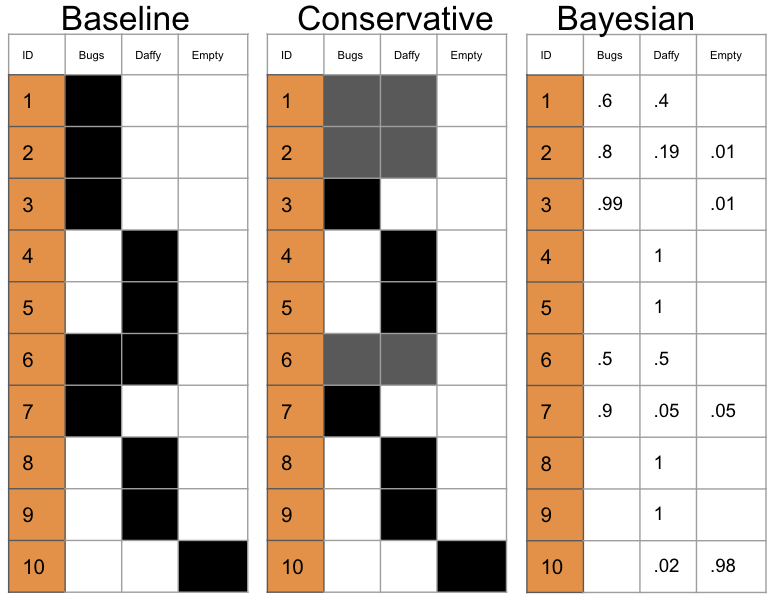
Figure 1: Generalization of normal CVR to the conservative setting where multiple interpretations are declared, and Bayesian setting where one associates probabilities with each interpretation. Blanks for the Bayesian setting have probability $0$.

1.2 A Detailed Survey of the General Framework and Our Results

As described above, a RLA is carried out in the context of an election with voter-verified ground truth. For concreteness, our discussion assumes hand-marked paper ballots, which is the most common instantiation in practice. The audit is intended to detect disagreement between the ground-truth outcome of the election, as determined by the ballots themselves, and the declared outcome of the election resulting from a tabulation of the ballots; we use the word “declared” throughout to emphasize that the tabulated outcome may be inconsistent with the ground-truth outcome. Such an audit examines a collection of physical ballots, usually drawn at random according to a convention depending on the audit, and either concludes with Consistent, indicating that the sampled ballots appear consistent with the declared outcome, or Inconclusive, indicating that the audit has not amassed sufficient evidence of consistency. An audit is said to have risk $\alpha$ (a number in the range $[0,1]$) if the probability that it outputs Consistent is no more than $\alpha$ when the declared outcome contradicts the ground-truth outcome.

A trivial audit that always outputs Inconclusive has zero risk, but is obviously not useful in practice. This points to the importance of completeness—the additional guarantee that the audit outputs Consistent with high probability under favorable circumstances; we discuss this in detail below. A straightforward hand recount of an election is itself a RLA audit with zero risk (modulo any errors in manual interpretation). More sophisticated RLAs randomly draw and inspect a collection of ballots to make statistical conclusions about the outcome. A general feature of such statistical audits is that the number of samples scales with the margin of victory; this reflects the natural intuition that a landslide should be easier to statistically verify than a victory by slim margin. In the most familiar setting of a simple, two-candidate, first-past-the-post election, the empirical mean of the number of votes for a particular candidate among a collection of $\log(2/\alpha)/(2\epsilon^{2})$ uniformly sampled ballots is correct to within $\epsilon$ with probability $1-\alpha$. This simple procedure—called “ballot polling” in the literature—yields a risk-limiting audit that inspects

$$O\left(\frac{\log(1/\alpha)}{\mu^{2}}\right)$$ (1)

ballots in expectation, where $\mu$ is the actual margin of victory [1].

The most efficient known approach for RLAs, known as a ballot comparison audit [1, 5, 6, 7, 9, 11, 12, 13], requires a detailed tabulation report called a CVR. A CVR declares a unique identifier and interpretation (that is, a determination of the cast votes) for each ballot in the election. This ballot-by-ballot record of the election naturally determines a tabulation and outcome. It also enables high-efficiency audits that proceed by iterating the following experiment: 1. The auditor picks a random identifier $\iota$ from the CVR table; 2. the auditor finds a physical ballot with identifier $\iota$; 3. the auditor compares the interpretation of the physical ballot against the associated CVR entry. Intuitively, iterations where the physical ballot matches the CVR provide support for this declared record of the election, while disagreements erode that support. Continuing the discussion in the same two-candidate first-past-the-post setting, observe that if the CVR table declares an incorrect outcome for the election, then at least a $\mu/2$ fraction of entries of the CVR table must disagree with the corresponding physical ballot; as above, $\mu$ is the scaled margin of ground-truth victory. (The factor of two arises because a single disagreement can both negate a vote for the declared winner and supply a vote for the declared loser.) It follows that after $2/\mu$ samples we expect to observe a discrepancy if the outcomes differ, suggesting that this approach should yield a risk-limiting audit with sample size

$$O\left(\frac{\log(1/\alpha)}{\mu}\right)\,.$$ (2)

(The $\log(1/\alpha)$ term increases the number of samples so that the probability of observing an inconsistency is driven to at least $1-\alpha$.) It is instructive to compare this against (1) above. Due to the improved dependence on $\mu$, in circumstances with small margins, ballot comparison is significantly more efficient than ballot polling.

The completeness challenge.

The efficiency landscape is more complicated than the discussion above (and the asymptotic expression (2)) indicates. The complication is the requirement of completeness—that is, that the audit conclude with Consistent when considering an accurate CVR under favorable conditions. In practice, when a post-election RLA concludes with Inconclusive, policy calls for either a complete hand count or an additional stage of auditing (with a smaller risk parameter so as to avoid significant amplification of risk from the composite audit). See for example Rhode Island legislation and Colorado’s fact sheet. Thus a full accounting of efficiency must weigh the costs and likelihood of Inconclusive conclusions in the best-effort settings that arise in practice.

To be more concrete, a ballot-comparison auditor simply wishing to meet a prescribed risk limit $\alpha$ could adopt the framework above with the convention that any observed disagreement between the CVR and a physical ballot causes the auditor to immediately terminate the audit and output Inconclusive. If examination of $\log(1/\alpha)/(2\mu)$ ballots indeed exposes no inconsistencies, the audit can safely return Consistent with only an $\alpha$ probability of error, as desired. For $\mu=.01$ and $\alpha=.05$, for example, this requires inspection of $499$ ballots. Now, if this “strict” auditor has the luxury of unambiguous ground truth, a perfectly correct CVR, and consistently accurate ballot interpretation, then it will indeed conclude the audit with Consistent. However, discrepancies between the CVR and physical ballots arise frequently in practice. (For example, the comparison RLA run by the US state of Colorado for the 2020 presidential election generated hundreds of discrepancies [22].) These discrepancies can result from truly ambiguous voter intent, disagreement among the interpretations of an auditing board, or operational errors such as retrieval of an incorrect ballot. Estimates from prior work (e.g. Stark’s audit tools; [23]) suggest discrepancy rates as large as $0.5\%$, though the actual rate of incidence depends on various features of the election.

These considerations have led to the adoption and development of audits (and associated statistical tests) that can tolerate such anticipated errors. For example, with these parameters (and continuing to use $\alpha=.05,\mu=.01$) the standard Kaplan-Markov test calls for a sample size of $1220$ ballots in order to terminate with probability 95%. This example illustrates that even small error rates have a drastic impact on required sample size; we remark, additionally, that the incidence of sporadic errors in an otherwise correct CVR is the cause of variance in the stopping time for such sequential statistical tests. As audits are typically conducted in phases—drawing a collection of ballots to be inspected at once and calibrated so that each phase is likely to be the last—variance also directly influences efficiency as it forces large phases.

These concerns motivate our exploration of more expressive CVRs. In particular, we note that the party (or tabulator) preparing the $\mathsf{cvr}$ can identify marginal marks during tabulation that are likely to lead to errors during a comparison audit. Reflecting these marginal marks on the CVR offers a new dimension of optimization for the auditing rule. As a matter of bookkeeping, we will consider CVRs that may list multiple interpretations for each ballot or a full predicted probability distribution of interpretations. (A traditional CVR corresponds to the case when the size of each set of interpretations is $1$.) We apply this to develop both conventional audits with improved efficiency and define a new class of competitive audits, providing both high efficiency and a mechanism for contesting conventional audits.

As we remarked above, enriching CVRs so that they have the expressive power to reflect marginal marks can also improve confidence in the audit, as it can distinguish unavoidable discrepancies arising from ambiguity from truly “unexplained” auditing failures.

1.2.1 Improved Efficiency Risk-Limiting Audits via Bayesian CVRs

We show how to adapt standard ballot comparison audits to the setting of Bayesian CVRs that declare a predicted distribution of ballot interpretations. We indicate how to formulate the standard notions of discrepancy and margin in this setting and observe that this simple change has significant efficiency ramifications. Using discrepancy and marginal rates from practice we show that such audits reduce sample size standard deviation by $14\%$ compared to a traditional audit at a margin of $1\%$ (see Table 2). We also develop a variant of this audit that uses a CVR that merely reflects the possible interpretations of each ballot (rather than a full probability distribution). While this does not provide the full benefits of the Bayesian approach, it may be simpler to deploy in practice since no probability estimation is required. It also considers a stronger adversarial model where the ballot interpretation of the auditor is adversarially controlled.

We adopt to our setting the cryptographic game-style modeling for RLAs developed in [15], and prove that the new audit is indeed risk-limiting. We then carry out simulations to show that the most popular sequential statistical test used for RLAs (the Kaplan-Markov test) can take advantage of the resulting notion of discrepancy to provide more efficient RLAs.

1.2.2 Competitive Audits and Election Contestation

Our second contribution is a new class of post-election audits that we call competitive RLAs. In a competitive RLA each candidate has an “advocate” that is allowed to examine ballots (under supervision to ensure ballots are not destroyed or modified). For each candidate $\mathsf{A}_{1},\ldots,\mathsf{A}_{k}$, their advocate produces a CVR that may declare different ballot interpretations and winners; the intent is that the advocate for candidate $\mathsf{A}$ files a CVR that is favorable to $\mathsf{A}$. In particular, if $\mathsf{A}$ won the election, the CVR (filed by the advocate for $\mathsf{A}$) should establish that; in a weaker sense, even if $\mathsf{A}$ did not win, the advocate may wish to file a CVR that prevents other candidates that did not win the election from claiming that they did. For simplicity, we formulate this audit in the “conservative” setting, where CVRs may list multiple interpretations for each ballot but do not record a probability distribution on these various possible interpretations. (It is certainly possible to formulate this in the setting with a Bayesian CVRs, see end of Section 6.)

Assuming that at least one submitted CVR only lists interpretations that are consistent with the ballots and the election has a winner, the auditor will identify the correct winner using a constant number of ballots. Furthermore, if some submitted CVR lists the exact list of possible interpretations for each ballot, no losing candidate can be identified as the winner. We emphasize that the number of ballot samples required by this approach is a constant that not scale with the margin. (The constant itself is a function of how robust the audit should be in the face of errors by the advocates.)

The basic idea of the audit is straightforward: Faced with a pair of contradictory CVRs—$\mathsf{cvr}_{1}$ and $\mathsf{cvr}_{2}$—there must be at least one ballot on which these CVRs completely disagree: examining this single ballot then provides an immediate strike against one of CVRs. Indeed, a strict auditor can use a generalization of this approach to settle the competing claims made by a collection of $k$ CVRs with just $k-1$ ballots. (That is, the auditor immediately removes from consideration any CVR found to be inconsistent with an inspected ballot.) Such a stringent auditor will not be appropriate in practice, which must account for a small number of errors on the part of the advocates (and the $\mathsf{cvr}_{i}$) or the possibility that ballots are lost, say, during the audit. Even accounting for such phenomena, our approach yields audits with remarkable efficiency. (As mentioned earlier, the complexity of the audit scales with the desired robustness in the face of such advocacy errors.)

The most natural and practical instantiation of our techniques is providing an efficient adjudication process for disagreements that result after the parallel scanning of ballots, for example, using the OpenScan system [24]. The idea of the OpenScan system is for advocates to place cameras above a physical scanner and create their own CVRs without having physical access to the ballots. Their system did not have a natural mechanism to adjudicate if the parties disagreed on the winner. Competitve audits provide that adjudication with a constant query ballot complexity.

Election contestation.

Competitive RLAs provide an immediate approach to election contestation. Specifically, consider a situation where a candidate wishes to dispute the conclusions of conventional RLA (that is, the candidate claims that an invalid election was not detected by the RLA). In this case, the candidate can be permitted to examine the ballots and produce a competing CVR for the election (that, presumably, will claim that the candidate is the victor). The CVR originally produced for the election (and reaffirmed by the original RLA) and the candidate’s CVR can then be treated by the competitive audit mechanism. This has a number of notable features: (i.) the audit can rigorously settle the dispute with risk $2^{-\theta(k)}$ after examining only $k$ ballots—thus a small constant number of queries are acceptable in practice. (ii.) this provides an interesting avenue for election policy: for example, the cost and effort of the audit could be borne by the contesting party.

Adversarial modeling.

As in the prior contribution, we consider an cryptographic game-based model for analysis. The model places the ballots (and, in fact, the choice of the returned interpretation) in the hands of an adversarial environment, thus reflecting properties of the audit in adverse circumstances that reflect a variety of the challenges that face practical audits.

Organization.

We cover notational preliminaries and define CVRs and ballots with multiple interpretations in Section 2, cover Bayesian audits in Section 3, Conservative audits in Section 4, evaluate efficiency of the Bayesian and conversative methods in Section 5, and competitive audits in Section 6.

2 Preliminaries; the Bayesian Setting

We use boldface to refer to “physical” objects, such as individual ballots (typically denoted $\mathbf{b}$) or groups of ballots (typically $\mathbf{B}$). For a natural number $k$, we define $[k]=\{1,\ldots,k\}$ (and $[0]=\emptyset$). We let $\Sigma=[-2,2]$, a set of particular significance as standard single-ballot discrepancy takes values in this set; this is discussed in detail later in the paper. For a set $X$, let $X^{*}$ be the set of all finite-length sequences over $X$; that is, $X^{*}=\{(x_{1},\ldots,x_{k})\mid k\geq 0,x_{i}\in X\}$. In particular, we let $\{0,1\}^{*}$ denote the collection of finite-length bitstrings. Finally, we define $X^{\mathbb{N}}$ to be the set of all sequences $\{(x_{0},x_{1},\ldots)\mid x_{i}\in X\}$. We typically use script letters, e.g., $\mathcal{P}$, to denote probability distributions.

Making multiple interpretations explicit requires many new definitions. A summary is in Table 1.

Formal definitions for ballots, elections, and cast-vote records.

For simplicity, we consider only audits of a single first-past-the-post race with a set $\mathcal{C}$ of candidates. See Stark [6, 11] for a detailed account of how more complex elections can be reduced to this canonical setting. We now set down the elementary definitions of elections, manifests, and CVRs. The main definitional change is that a physical ballot yields a probability distribution of possible outcomes; this models the important situation where a physical ballot may have ambiguous markings that could reasonably be interpreted in various ways by an auditing board or a tabulation device. We explore two conventions for cast vote records to reflect this uncertainty: the first is the Bayesian framework, which associates with each ballot a predicted probability distribution of possible readings (depending on the anticipated reading a particular audit board, say). We then formulate a simpler, conservative model that posits a collection of interpretations for each ballot without assigning them probabilities. This reduces the complexity of producing cast-vote records, as one only needs to identify the possible interpretations of a ballot rather than a comprehensive probability distribution. In this conservative model, we consider quite strong adversarial behavior that assumes that the audit board always returns the “worst-case” interpretation allowed by the ballot. (In fact, this is equivalent to replacing the probabilities listed on the CVR with a probability of $1$ for some interpretation that “minimizes” the margin for a declared winner.) To move as swiftly as possible to our results on conventional audits with marginal marks, we first lay out the definitions for the Bayesian case; we return to the definitions for the conservative case in Section 6.

Definition 1 (Interpretations, ballots, and ballot families).

Let $\mathcal{C}$ be a set of candidates. An interpretation is a function $I:\mathcal{C}\rightarrow\{0,1\}$; when $\mathcal{C}$ is understood from context, we write $\mathcal{I}=\{I:\mathcal{C}\rightarrow\{0,1\}\}$ for the collection of all interpretations. Such interpretations will be used to indicate the votes appearing for candidates on individual ballots. A ballot is a physical object $\mathbf{b}$ with two properties:

1. The ballot $\mathbf{b}$ is labeled with an indelible identifier $\operatorname{id}_{\mathbf{b}}\in\{0,1\}^{*}$.

2. The ballot $\mathbf{b}$ determines a “ground truth” probability distribution $\mathcal{T}_{\mathbf{b}}$ on the set of interpretations $\mathcal{I}$. Thus $\mathcal{T}_{\mathbf{b}}:\mathcal{I}\rightarrow\mathbb{R}$ is a non-negative function on $\mathcal{I}$ for which $\sum_{I\in\mathcal{I}}\mathcal{T}_{\mathbf{b}}(I)=1$.

We let $\mathsf{T}_{\mathbf{b}}^{{\scriptsize{\LEFTcircle}}}:\mathcal{C}\rightarrow\mathbb{R}$ denote the expected interpretation over the distribution $\mathcal{T}_{\mathbf{b}}$: that is, for each $\mathsf{A}\in\mathcal{C}$, $\mathsf{T}_{\mathbf{b}}^{{\scriptsize{\LEFTcircle}}}(\mathsf{A})=\operatorname{\mathbb{E}}[{\mathrm{I}}_{\mathbf{b}}(\mathsf{A})]\,,$ where ${\mathrm{I}}_{\mathbf{b}}$ is a random variable distributed according to $\mathcal{T}_{\mathbf{b}}$.

A ballot family $\mathbf{B}$ is a collection of ballots with the same candidates. We let $\mathbf{B}_{\iota}=\{\mathbf{b}\in\mathbf{B}\mid\operatorname{id}_{\mathbf{b}}=\iota\}$ denote the subset of ballots with identifier $\iota$. When ballots identifiers are distinct across $\mathbf{B}$, so that $|\mathbf{B}_{\iota}|\leq 1$ for each $\iota$, we say that the family is uniquely labeled.

Ballots are typically intended to have an unambiguous interpretation. This corresponds to the case where the distribution $\mathcal{T}_{\mathbf{b}}$ is supported on a single interpretation (taking the value 1 at that interpretation and zero elsewhere).

Definition 2.

An election $E$ is a tuple $(\mathcal{C},\mathbf{B},\mathsf{S})$ where $\mathcal{C}$ is a set of candidates, $\mathbf{B}$ is a ballot family, and $\mathsf{S}=|\mathbf{B}|$ is the total number of ballots.

Definition 3 (Election winners, losers, and margin).

Let $E=(\mathcal{C},\mathbf{B},\mathsf{S})$ be an election. For a candidate $\mathsf{A}\in\mathcal{C}$, define

$$E^{\scriptsize{\LEFTcircle}}(\mathsf{A})=\sum_{\mathbf{b}\in\mathbf{B}}\mathsf{T}_{\mathbf{b}}^{\scriptsize{\LEFTcircle}}(A).$$

The margin of $\mathsf{A}$ with respect to $\mathsf{B}$ is defined to be

$$\mu_{\mathsf{A},\mathsf{B}}=\frac{E^{{\scriptsize{\LEFTcircle}}}(\mathsf{A})-E^{{\scriptsize{\LEFTcircle}}}(\mathsf{B})}{\mathsf{S}}.$$

When we wish to emphasize that this notion of margin is defined with respect to the expected values $\mathsf{T}_{\mathbf{b}}^{\scriptsize{\LEFTcircle}}(\cdot)$ we refer to it as Bayesian margin. A candidate $\mathsf{W}\in\mathcal{C}$ is the winner of the election $E$ if $\forall\mathsf{A}\in\mathcal{C}\setminus\{\mathsf{W}\},\mu_{\mathsf{W},\mathsf{A}}>0$. In this case, we define the margin, denoted $\mu$, of the election to be the minimum of these quantities:

$$\mu_{E}=\min_{\mathsf{A}\in\mathcal{C}\setminus\{\mathsf{W}\}}\mu_{\mathsf{W},\mathsf{A}}\,.$$

Otherwise, the election does not determine a winner and we define $\mu_{E}:=0$. If a winner exists it is unique. A candidate $\mathsf{L}$ is called a loser if there is a candidate $\mathsf{A}$ for which $E^{{\scriptsize{\LEFTcircle}}}(\mathsf{L})<E^{{\scriptsize{\LEFTcircle}}}(\mathsf{A})$.

Cast-vote record (CVR).

A cast-vote record table (CVR) is an (untrusted) declaration of both the ballots appearing in an election and the interpretations of the ballots.

Definition 4 (Bayesian Cast-Vote Record Table).

Let $\mathcal{C}$ be a set of candidates. A Bayesian Cast-Vote Record table (CVR) is a sequence of pairs

$$\mathsf{cvr}=\bigl{(}(\iota_{1},\mathcal{P}_{1}),\ldots,(\iota_{t},\mathcal{P}_{t})\bigr{)}$$

where the $\iota_{r}$ are distinct bitstrings in $\{0,1\}^{*}$ and each $\mathcal{P}_{r}:\mathcal{I}\rightarrow\mathbb{R}$ is a probability distribution on $\mathcal{I}$ which we refer to as a “prediction.” Intuitively, such a $\mathsf{cvr}$ declares that, for each row $r$, the interpretation of the ballot labeled $\iota_{r}$ is given by the distribution $\mathcal{P}_{r}$.

For each candidate $\mathsf{A}\in\mathcal{C}$ and $r\in\{1,\ldots,t\}$, we define $\mathsf{P}^{{\scriptsize{\LEFTcircle}}}_{r}(\mathsf{A})=\operatorname{\mathbb{E}}[I(\mathsf{A})]$, the expected value of the vote for $\mathsf{A}$ when $I$ is drawn according to the distribution $\mathcal{P}_{r}$. We then define

$$\qquad\mathsf{cvr}(\mathsf{A})=\sum_{r=1}^{t}\mathsf{P}^{{\scriptsize{\LEFTcircle}}}_{r}(\mathsf{A})\,.$$

Declared winners and losers.

If there is a candidate $\mathsf{A}\in\mathcal{C}$ with the property that $\mathsf{cvr}(\mathsf{A})>\mathsf{cvr}(\mathsf{B})$ for every $\mathsf{B}\in\mathcal{C}\setminus\{\mathsf{A}\}$, then we say that $\mathsf{A}$ is the declared winner according to $\mathsf{cvr}$. A candidate $\mathsf{A}$ for which there exists some $\mathsf{B}$ such that $\mathsf{cvr}(\mathsf{A})<\mathsf{cvr}(\mathsf{B})$ is called a declared loser.

We use the following general language when referring to CVRs:

1. The bitstrings $\iota_{r}$ are identifiers and we let $\mathtt{Idents}(\mathsf{cvr})$ denote this set.

2. The number $t$ is the size of the CVR.

3. The $r$th row, denoted $\mathsf{cvr}(r)$, refers to the tuple $(\iota_{r},\mathcal{P}_{r})$.

4. Identifiers appearing in the CVR are distinct, so when convenient we reference $\mathcal{P}_{r}$ and $\mathsf{P}_{r}$ by identifier rather than row: that is, for an identifier $\iota=\iota_{r}$ appearing in the CVR, we define $\mathcal{P}_{\iota}:=\mathcal{P}_{r}$ and $\mathsf{P}_{\iota}^{{\scriptsize{\LEFTcircle}}}:=\mathsf{P}_{r}^{{\scriptsize{\LEFTcircle}}}$.

Definition 5 (Bayesian declared margin).

Let $\mathsf{cvr}$ be a Bayesian CVR with declared winner $\mathsf{W}$ and size $s$. The declared margin of $\mathsf{cvr}$ is the quantity

$$\mu_{\mathsf{cvr}}:=\min_{\mathsf{A}\in\mathcal{C}\setminus\mathsf{W}}\frac{\mathsf{cvr}(\mathsf{W})-\mathsf{cvr}(\mathsf{A})}{s}\geq 0.$$

If $\mathsf{cvr}$ has no declared winner, we define $\mu_{\mathsf{cvr}}:=0$.

Definition 6 (Bayesian validity, consistency, and contradiction).

Let $E=(\mathcal{C},\mathbf{B},\mathsf{S})$ be an election and $\mathsf{cvr}$ be a Bayesian CVR. We say that $\mathsf{cvr}$ is valid for $E$ if $E$ has a winner and $\mathsf{cvr}$ declares that winner. We say that $\mathsf{cvr}$ is invalid for $E$ if it declares a winner $\mathsf{W}$ that does not win $E$.

Definition 7 (Bayesian discrepancy).

Let $E=(\mathcal{C},\mathbf{B},\mathsf{S})$ be an election and let $\mathsf{cvr}=((\iota_{1},\mathcal{P}_{1}),\ldots,(\iota_{t},\mathcal{P}_{t}))$ be a Bayesian CVR with declared winner $\mathsf{W}$. For a ballot $\mathbf{b}\in\mathbf{B}$ and a distribution $\mathcal{P}:\mathcal{I}\rightarrow\mathbb{R}$, the discrepancy is

$$\mathsf{D}[\mathcal{P},\mathbf{b};\mathsf{W}]=\max_{\mathsf{A}\in\mathcal{C}\setminus\mathsf{W}}\left(\bigl{(}\mathsf{P}^{{\scriptsize{\LEFTcircle}}}(\mathsf{W})-\mathsf{P}^{{\scriptsize{\LEFTcircle}}}(\mathsf{A})\bigr{)}-\bigl{(}\mathsf{T}^{{\scriptsize{\LEFTcircle}}}_{\mathbf{b}}(\mathsf{W})-\mathsf{T}^{{\scriptsize{\LEFTcircle}}}_{\mathbf{b}}(\mathsf{A})\bigr{)}\right)$$

where, as above, $\mathsf{P}^{{\scriptsize{\LEFTcircle}}}(\mathsf{A})=\operatorname{\mathbb{E}}[I(\mathsf{A})]$ with $I$ distributed according to $\mathcal{P}$. We expand this definition to apply, additionally, to a special symbol $\mathbf{\bot}$:

$$\mathsf{D}[\mathcal{P},\perp;\mathsf{W}]=\max_{\mathsf{A}\in\mathcal{C}\setminus\mathsf{W}}\left(\mathsf{P}^{{\scriptsize{\LEFTcircle}}}(\mathsf{W})-\mathsf{P}^{{\scriptsize{\LEFTcircle}}}(\mathsf{A})\right)+1\,.$$

For an identifier $\iota$ define

$$\mathsf{D}_{\mathsf{cvr},\iota}=\begin{cases}\min\;\bigl{\{}\mathsf{D}[\mathcal{P}_{\iota},\mathbf{b};\mathsf{W}]\mid\mathbf{b}\in\mathbf{B}_{\iota}\bigr{\}}&\text{if $\mathbf{B}_{\iota}\neq\emptyset$,}\\ \mathsf{D}[\mathcal{P}_{\iota},\bot;\mathsf{W}]&\text{otherwise.}\end{cases}$$

The discrepancy of the cast vote record table $\mathsf{cvr}$ is: $\mathsf{D}_{\mathsf{cvr}}=\sum_{i=1}^{t}\mathsf{D}_{\mathsf{cvr},\iota_{i}}.$

We begin by establishing the fundamental relationship between discrepancy and margin for invalid CVRs.

Audit Type	Notation	Meaning
All	$\mathbf{b}$	Physical ballot
	$\mathbf{B}$	Ballot family
	$\mathbf{B}_{\iota}$	Ballots with identifier $\iota$
	$\mathsf{S}$	Number of ballots in election
	$\mathcal{C}$	Candidates in the election
Bayesian	$E$	Election
	$\mathcal{T}_{\mathbf{b}}$	Probability distribution over auditor interpretation of ballot $\mathbb{b}$
	${\mathrm{I}}_{\mathbf{b}}$	Random variable with distribution $\mathcal{T}_{\mathbf{b}}$
	$\mathsf{T}_{\mathbf{b}}^{{\scriptsize{\LEFTcircle}}}(\mathsf{A})$	Expected number of votes for ballot $\mathbf{b}$ received by candidate $\mathsf{A}$ if audited
	$E^{\scriptsize{\LEFTcircle}}(\mathsf{A})$	Expected number of votes across election received by candidate $\mathsf{A}$ if hand counted
	$\mathcal{P}_{r}$	Predicted distribution of interpretations for ballot with identifier $r$
	$\mathsf{P}^{{\scriptsize{\LEFTcircle}}}_{r}(\mathsf{A})$	Expected number of votes predicted for candidate $\mathsf{A}$ on ballot with identifier $r$
	$\mu_{\mathsf{A},\mathsf{B}}$	Bayesian diluted margin of $\mathsf{A}$ with respect to candidate $\mathsf{B}$
	$\mu_{\mathsf{A}}$	Minimum of Bayesian diluted margin across candidates
	$\mathsf{cvr}$	Cast vote record containing identifiers and predicted interpretation distributions for each ballot
	$\mathsf{cvr}(\mathsf{A})$	Predicted number of votes received by $\mathsf{A}$ on $\mathsf{cvr}$
	$\mu_{\mathsf{cvr}}$	Bayesian diluted margin declared by $\mathsf{cvr}$
	$\mathsf{D}_{\mathsf{cvr}}$	Discrepancy of $\mathsf{cvr}$ with respect to election $E$
Conservative	$T_{\mathbf{b}}$	Set of possible interpretations on $\mathbf{b}$
	$T^{{\scriptsize{\CIRCLE}}}_{\mathbf{b}}(\mathsf{A})$	Best interpretation for $\mathsf{A}$ on $\mathbf{b}$
	$T^{{\scriptsize{\Circle}}}_{\mathbf{b}}(\mathsf{A})$	Worst interpretation for $\mathsf{A}$ on $\mathbf{b}$
	$T^{{\scriptsize{\CIRCLE}}}(\mathsf{A})$	Most possible votes for $\mathsf{A}$ in election
	$T^{{\scriptsize{\Circle}}}(\mathsf{A})$	Least possible votes for $\mathsf{A}$ in election
	$\mu_{\mathsf{A},\mathsf{B}}^{+}$	Conservative diluted margin of $\mathsf{A}$ with respect to candidate $\mathsf{B}$
	$\mu_{\mathsf{A}}^{+}$	Minimum of Conservative diluted margin across candidates
	$\mu_{\mathsf{cvr}}^{+}$	Conservative diluted margin declared by $\mathsf{cvr}^{+}$
	$\mathsf{cvr}^{+}$	Conservative $\mathsf{cvr}$ declaring set of possible interpretations
	$\mathsf{P}^{{\scriptsize{\Circle}}}_{r}(\mathsf{A})$	Worst predicted interpretation for candidate $\mathsf{A}$
	$\mathsf{P}^{{\scriptsize{\CIRCLE}}}_{r}(\mathsf{A})$	Best predicted interpretation for candidate $\mathsf{A}$
	$\mathsf{cvr}^{{\scriptsize{\Circle}}}(\mathsf{A})$	Minimum votes for $\mathsf{A}$ on $\mathsf{cvr}$
	$\mathsf{cvr}^{{\scriptsize{\CIRCLE}}}(\mathsf{A})$	Maximum votes for $\mathsf{A}$ on $\mathsf{cvr}$
	$\mathsf{D}_{\mathsf{cvr}}^{+}$	Conservative discrepancy of $\mathsf{cvr}$ with respect to election $E$
Competitive	$\mathtt{Omission}(\mathsf{cvr}_{\mathsf{A}},\mathsf{cvr}_{\mathsf{B}})$	Set of identifiers declared by $\mathsf{cvr}_{\mathsf{A}}$ absent in $\mathsf{cvr}_{\mathsf{B}}$
	$\mathtt{Conflict}(\mathsf{cvr}_{\mathsf{A}},\mathsf{cvr}_{\mathsf{B}})$	Set of identifiers that appear in both CVRs with no interpretations in common
	$\mathtt{Disagree}(\mathsf{cvr}_{\mathsf{A}},\mathsf{cvr}_{\mathsf{B}})$	Union of omission and conflict

Table 1: Summary of Notation

Lemma 1.

Let $E=(\mathcal{C},\mathbf{B},\mathsf{S})$ be an election and let $\mathsf{cvr}$ be an invalid CVR for $E$ with declared winner $\mathsf{W}$ and size $t=\mathsf{S}$. Then $\mathsf{D}_{\mathsf{cvr}}\geq(\mu_{\mathsf{cvr}}+\mu_{E})\cdot\mathsf{S}\geq\mu_{\mathsf{cvr}}\cdot\mathsf{S}$.

Proof of Lemma 1.

Let $\mathtt{Idents}^{R}$ denote the subset of identifiers that identify least one ballot: that is, $\mathtt{Idents}^{R}=\{\iota\in\mathtt{Idents}(\mathsf{cvr})\mid\mathbf{B}_{\iota}\neq\emptyset\}$. We call these “represented” identifiers. For each $\iota\in\mathtt{Idents}^{R}$, let $\mathbf{c}_{\iota}$ be a ballot in $\mathbf{B}_{\iota}$ for which $\mathsf{D}[\mathcal{P}_{\iota},\mathbf{c}_{\iota};\mathsf{W}]=\mathsf{D}_{\mathsf{cvr},\iota}$. As $\mathbf{B}_{\iota}\cap\mathbf{B}_{\iota^{\prime}}=\emptyset$ for any $\iota\neq\iota^{\prime}$, these chosen ballots $\mathbf{c}_{\iota}$ are distinct. Considering that $|\mathtt{Idents}(\mathsf{cvr})|=t=\mathsf{S}=|\mathbf{B}|$, the number of “unassigned” ballots in $\mathbf{B}$ (that do not appear in $\{\mathbf{c}_{\iota}\mid\iota\in\mathtt{Idents}^{R}\}$) is the same as the number of unrepresented identifiers (appearing in $\mathtt{Idents}(\mathsf{cvr})$ but not in $\mathtt{Idents}^{R}$). By choosing an arbitrary one-to-one correspondence between unrepresented identifiers and unassigned ballots, we may extend the correspondence $\iota\leftrightarrow\mathbf{c}_{\iota}$ to all identifiers in $\mathtt{Idents}(\mathsf{cvr})$ and all ballots in $\mathbf{B}$ so that it is a one-to-one correspondence between these two sets.

To complete the proof, we observe that

$$\mathsf{D}_{\mathsf{cvr}} =\sum_{i=1}^{t}\mathsf{D}_{\mathsf{cvr},\iota_{i}}$$ (3)

$$=\;\;\sum_{\mathclap{\iota\in\mathtt{Idents}^{R}}}\min\left\{\mathsf{D}[\mathcal{P}_{\iota},\mathbf{b};\mathsf{W}]\mid\mathbf{b}\in\mathbf{B}_{\iota}\right\}+\sum_{\mathclap{\begin{subarray}{c}\iota\not\in\mathtt{Idents}^{R}\\ (\iota\in\mathtt{Idents}(\mathsf{cvr}))\end{subarray}}}\mathsf{D}[\mathcal{P}_{\iota},\bot;\mathsf{W}]$$

$$\geq\;\;\sum_{\mathclap{\iota\in\mathtt{Idents}^{R}}}\mathsf{D}[\mathcal{P}_{\iota},\mathbf{c}_{\iota};\mathsf{W}]+\sum_{\mathclap{\begin{subarray}{c}\iota\not\in\mathtt{Idents}^{R}\\ (\iota\in\mathtt{Idents}(\mathsf{cvr}))\end{subarray}}}\mathsf{D}[\mathcal{P}_{\iota},\mathbf{c}_{\iota};\mathsf{W}]$$

$$\geq\;\;\sum_{\mathclap{\iota\in\mathtt{Idents}}}\mathsf{D}[\mathcal{P}_{\iota},\mathbf{c}_{\iota};\mathsf{W}]\,,$$ (4)

where we have used the fact—immediate from the definition—that for any distribution $\mathcal{P}$ and any ballot $\mathbf{b}$,

$$\mathsf{D}[\mathcal{P},\bot;\mathsf{W}]\geq\mathsf{D}[\mathcal{P},\mathbf{b};\mathsf{W}]\,.$$

Let $\mathsf{B}\neq\mathsf{W}$ be a candidate for which $E^{{\scriptsize{\LEFTcircle}}}(\mathsf{B})\geq E^{{\scriptsize{\LEFTcircle}}}(\mathsf{A})$ for all candidates $\mathsf{A}$. (If there is no winner in $E$, such a candidate always exists but may “tie” with some other candidate(s).) Then, again by the definition of discrepancy, for each $\iota$

$$\mathsf{D}[\mathcal{P}_{\iota},\mathbf{c}_{\iota};\mathsf{W}]\geq\left(\bigl{(}\mathsf{P}^{{\scriptsize{\LEFTcircle}}}_{\iota}(\mathsf{W})-\mathsf{P}^{{\scriptsize{\LEFTcircle}}}_{\iota}(\mathsf{B})\bigr{)}-\bigl{(}\mathsf{T}^{{\scriptsize{\LEFTcircle}}}_{\mathbf{c}_{\iota}}(\mathsf{W})-\mathsf{T}^{{\scriptsize{\LEFTcircle}}}_{\mathbf{c}_{\iota}}(\mathsf{B})\bigr{)}\right)$$

Returning to the expression (4), we then conclude that

$$\sum_{\mathclap{\iota\in\mathtt{Idents}(\mathsf{cvr})}}\;\mathsf{D}[\mathcal{P}_{\iota},\mathbf{c}_{\iota};\mathsf{W}] \geq\sum_{i}\left(\begin{subarray}{c}\bigl{(}\mathsf{P}^{{\scriptsize{\LEFTcircle}}}_{\iota}(\mathsf{W})-\mathsf{P}^{{\scriptsize{\LEFTcircle}}}_{\iota}(\mathsf{B})\bigr{)}+\\ \bigl{(}\mathsf{T}^{{\scriptsize{\LEFTcircle}}}_{\mathbf{c}_{\iota}}(\mathsf{B})-\mathsf{T}^{{\scriptsize{\LEFTcircle}}}_{\mathbf{c}_{\iota}}(\mathsf{W})\bigr{)}\end{subarray}\right)$$

$$=\begin{subarray}{c}\sum_{i}\bigl{(}\mathsf{P}^{{\scriptsize{\LEFTcircle}}}_{\iota}(\mathsf{W})-\mathsf{P}^{{\scriptsize{\LEFTcircle}}}_{\iota}(\mathsf{B})\bigr{)}+\\ \sum_{\mathbf{b}\in\mathbf{B}}\bigl{(}\mathsf{T}^{{\scriptsize{\LEFTcircle}}}_{\mathbf{b}}(\mathsf{B})-\mathsf{T}^{{\scriptsize{\LEFTcircle}}}_{\mathbf{b}}(\mathsf{W})\bigr{)}\end{subarray}$$

$$=\bigl{(}\mathsf{cvr}(\mathsf{W})-\mathsf{cvr}(\mathsf{B})\bigr{)}+\bigl{(}E(\mathsf{B})-E(\mathsf{W})\bigr{)}$$

$$\geq\mathsf{S}\cdot(\mu_{\mathsf{cvr}}+\mu_{E})\,.$$

In the first equality above we use the fact that $\iota\leftrightarrow\mathbf{c}_{\iota}$ is a one-to-one correspondence, so that each ballot appears once in this sum. We conclude that $\mathsf{D}_{\mathsf{cvr}}\geq\mathsf{S}(\mu_{\mathsf{cvr}}+\mu_{E})$, as desired. ∎

3 Bayesian Comparison Audits; Leveraging Marginal Marks

We present our auditor and analysis using a cryptographic game between the auditor and the environment, in the spirit of [15]. The auditor naturally reflects the role played by an auditing team in a conventional audit; as such it is provided with a CVR, the actual size of the election (in real-world settings this is provided by a trusted ballot manifest), and the ability to request ballots by identifier in order to carry out the audit. When the auditor has completed the audit, it returns either the token Inconclusive or Consistent. The environment, on the other hand, is responsible for providing physical ballots when they are requested. Note, in particular, that the auditor’s access to ballots is entirely mediated by the environment, which may choose not to return ballots when they are requested, make choices about which ballot to return when multiple ballots share an identifier, etc. The power of this modeling framework is that the critical concept of risk can be defined in the worst case over all possible behaviors of the environment. This reflects a wide variety of failures—inadvertent or malicious—that occur in practical audits.

The formal Auditor-Environment game is described in Figure 2. We remark that each ballot “delivered” by the environment in the game generates a single draw from the associated ground truth distribution of interpretations; multiple requests for the same ballot are permitted by the convention, which generate new independent samples from the ground truth distribution (modeling a situation where an audit board evaluates the ballot afresh each time it is sampled).

The formal auditor.

The auditor we consider is a standard “comparison auditor” adapted to the setting where discrepancy is computed with respect to the expected value of the predicted distribution in the CVR rather than a single interpretation. Fortunately, once discrepancy is redefined in this way, the remaining analysis of the standard auditor requires no significant changes. We lay down the definitions below.

The precise definition of an auditor requires specifying a “one-sided” statistical test. To explain the intuition, consider a situation where an auditor is provided an invalid CVR with declared margin $\mu_{\mathsf{cvr}}$. From Lemma 1, the straightforward ballot comparison experiment calling for the auditor to sample a random identifier from the CVR and compare the interpretation of the returned ballot to the predicted distribution on the CVR yields discrepancy $\mathsf{D}$ for which $\operatorname{\mathbb{E}}[\mathsf{D}]\geq\mu_{\mathsf{cvr}}$. Of course, a valid CVR that accurately reflects the interpretations on the ballots will be able to achieve $\operatorname{\mathbb{E}}[\mathsf{D}]\approx 0$. Thus, the auditor wishes to ensure that if $\operatorname{\mathbb{E}}[\mathsf{D}]\geq\mu_{\mathsf{cvr}}$ it will only return the token Consistent with small probability $\alpha$ (the “risk” of the audit). This is precisely the task of a “one-sided” statistical test. In fact, as we consider environments that need not respond independently during each ballot request, we require a slightly richer family of tests, formulated in this setting by [15]. We briefly lay out the definitions here, noting these definitions are used in a similar manner.

Auditor ($\mathtt{MAudit}$)–Environment ($\mathtt{Env}$) game for election $E=(\mathbf{B},\mathcal{C},\mathsf{S})$ and CVR $\mathsf{cvr}$

1. Setup.

   1. Ballot and tabulation delivery (to $\mathtt{Env}$). The physical ballots $\mathbf{B}$ is given to $\mathtt{Env}$.

   2. Ballot manifest and CVR delivery (to $\mathtt{MAudit}$). The size $\mathsf{S}$ and the $\mathsf{cvr}$ are given to the auditor $\mathtt{MAudit}$.

2. Audit. $\mathtt{MAudit}$ repeatedly makes a ballot request to $\mathtt{Env}$, or chooses to conclude the audit:

   A ballot request. $\mathtt{MAudit}$ requests a ballot from $\mathtt{Env}$ with identifier $\iota\in\{0,1\}^{*}$.

   $\mathtt{Env}$ does one of two things:

   1. Responds with a ballot $\mathbf{b}$ with identifier $\iota^{\prime}$; in this case, $\mathtt{MAudit}$ is given $\iota^{\prime}$ and $I$, an interpretation drawn from $\mathcal{T}_{\mathbf{b}}$.

   2. Responds with No ballot; this is forwarded to $\mathtt{MAudit}$.

3. Conclusion. $\mathtt{MAudit}$ returns one of the two values: Consistent or Inconclusive.

Figure 2: The $\mathsf{RLA}_{\mathtt{MAudit},\mathtt{Env}}(E,\mathsf{cvr})$ auditing game for comparison audits with multiple interpretations.

Definition 8.

[15, Definition 8] A sequence of bounded (real-valued) random variables $X_{1},\ldots$ are said to be $\delta$-dominating if, for each $t\geq 0$, $\operatorname{\mathbb{E}}[X_{t}\mid X_{1},\ldots,X_{t-1}]\geq\delta\,.$ We apply this terminology to the distribution $\mathcal{D}$ corresponding to the random variables, writing $\delta\unlhd\mathcal{D}$.

Definition 9.

[15, Definition 9] Let $\Sigma=[-2,2]$. A stopping time is a function $\mathsf{Stop}:\Sigma^{*}\rightarrow\{0,1\}$ so that for any sequence $x_{1},x_{2},\ldots$ of values in $\Sigma$ there is a finite prefix $x_{1},\ldots,x_{k}$ for which $\mathsf{Stop}(x_{1},\ldots,x_{k})=1$.

For a sequence of random variables $X_{1},\ldots$ taking values in $\Sigma$, let $\tau_{\mathsf{Stop}}(X_{1},\ldots)$ be the random variable given by the smallest $t$ for which $\mathsf{Stop}(X_{1},\ldots,X_{t})=1$. This naturally determines the random variable $X_{1},\ldots,X_{\tau_{\mathsf{Stop}}}$, the prefix of the $X_{i}$ given by the first time $\mathsf{Stop}()=1$.

Definition 10.

[15, Definition 10] An adaptive audit test, denoted $T=(\mathsf{Stop},\mathsf{R})$, is described by two families of functions, $\mathsf{Stop}_{\delta}$ and $\mathsf{R}_{\delta}$. For each $0<\delta\leq 1$,

1. $\mathsf{Stop}_{\delta}$ is a stopping time, as in Definition 9, and

2. $\mathsf{R}_{\delta}:\Sigma^{*}\rightarrow\{0,1\}$ is the rejection criterion.

Let $\mathcal{D}$ be a probability distribution on $\Sigma^{\mathbb{N}}$; for such a distribution, define $\alpha_{\delta,{\mathcal{D}}}=\operatorname{\mathbb{E}}[\mathsf{R}_{\delta}(X_{1},\ldots,X_{\tau})]$ where $X_{1},\ldots$ are random variables distributed according to $\mathcal{D}$ and $\tau$ is determined by $\mathsf{Stop}_{\delta}$. The risk of the test $T$ is

$$\alpha=\sup_{\begin{subarray}{c}0<\delta\leq 2\\ \delta\unlhd\mathcal{D}\end{subarray}}\alpha_{\delta,{\mathcal{D}}}\,.$$ (5)

The formal auditor for the Bayesian setting is presented in Figure 3, and depends on a particular adaptive statistical test. As mentioned above, the auditor is the natural comparison auditor [1]; the key difference with existing approaches is that computation of margin and discrepancy incorporates Bayesian CVR predictions.

$\mathtt{MAudit}[\mathsf{Stop},\mathsf{R}](E=(\mathcal{C},\mathbf{B},\mathsf{S}),\mathsf{cvr})$

1. Receive $\mathsf{cvr}=\bigl{(}(\iota_{1},\mathcal{P}_{1}),\ldots,(\iota_{t},\mathcal{P}_{t})\bigr{)}$.

2. If $\mathsf{cvr}$ has repeated identifiers or $\mathsf{S}\neq t$, return Inconclusive.

3. If $\mathsf{cvr}$ declares a winner $\mathsf{W}$, define $\mu:=\mu_{\mathsf{cvr}}$;
   otherwise, return Inconclusive.

4. Initialize $\mathsf{iter}=0$.

5. Repeat

   1. Increment $\mathsf{iter}:=\mathsf{iter}+1$.

   2. Perform $\mathsf{D}_{\mathsf{iter}}:=\mathtt{BasicExperiment}$

   until $\mathsf{Stop}_{\mu}(\mathsf{D}_{1},...,\mathsf{D}_{\mathsf{iter}})=1$

6. If $\mathsf{R}_{\mu}(\mathsf{D}_{1},...,\mathsf{D}_{\mathsf{iter}})=1$ return $\mathtt{Consistent}$; otherwise return Inconclusive.

$\mathtt{BasicExperiment}$:

1. $\mathtt{RowSelect}$: Select a row $r\in[\mathsf{S}]$ uniformly.

2. Let $\iota$ be the identifier in row $r$; request delivery of $\iota$.

3. If a ballot $\mathbf{b}$ was delivered with identifier $\iota^{\prime}=\iota$ and interpretation $I^{*}$, return

   $$\mathrm{act}:=\max_{\mathsf{A}\in\mathcal{C}\setminus\mathsf{W}}\left(\mathsf{P}^{{\scriptsize{\LEFTcircle}}}_{r}(\mathsf{W})-\mathsf{P}^{{\scriptsize{\LEFTcircle}}}_{r}(\mathsf{A})-\left(I^{*}(\mathsf{W})-I^{*}(\mathsf{A})\right)\right).$$

   Else, return $\displaystyle\mathrm{act}:=\max_{\mathsf{A}\in\mathcal{C}\setminus\mathsf{W}}\left(\mathsf{P}^{{\scriptsize{\LEFTcircle}}}_{r}(\mathsf{W})-\mathsf{P}^{{\scriptsize{\LEFTcircle}}}_{r}(\mathsf{A})\right)-1$.

Figure 3: The auditor $\mathtt{MAudit}[(\mathsf{Stop},\mathsf{R})]$.

We can now define the risk of a Bayesian audit.

Definition 11 (Risk of Bayesian audit).

Let $\mathtt{MAudit}$ be an Auditor. For election $E$ and environment $\mathtt{Env}$ let $\mathsf{RLA}_{\mathtt{MAudit},\mathtt{Env}}(E)$ denote the random variable equal to the conclusion of the audit as described in Figure 2. An auditor $\mathtt{MAudit}$ has $\alpha$-risk (or $\alpha$-soundness) if, for all elections $E$, all invalid $\mathsf{cvr}$s and all environments $\mathtt{Env}$,

$$\Pr_{\mathtt{MAudit},\mathtt{Env}}[\mathsf{RLA}_{\mathtt{MAudit},\mathtt{Env}}(E,\mathsf{cvr})=\textsc{Consistent}]\leq\alpha\,.$$

Theorem 1.

Let $E$ be an election and $\mathsf{cvr}$ be an invalid CVR. For any environment $\mathtt{Env}$, let $\mathsf{D}^{\mathrm{obs}}_{i,\mathtt{Env}}$ denote the random variable computed in $\mathtt{BasicExperiment}$ during iteration $i$; then $\mathbb{E}[\mathsf{D}^{\mathrm{obs}}_{i,\mathtt{Env}}]\geq\mathsf{D}_{\mathsf{cvr}}/\mathsf{S}\geq\mu_{\mathsf{cvr}}$.

Let $(\mathsf{Stop},\mathsf{R})$ be an adaptive audit test with risk $\alpha$. Let $\mathtt{MAudit}$ be as in Figure 3, $\mathtt{MAudit}[\mathsf{Stop},\mathsf{R}]$ has risk $\alpha$.

Proof.

The proof of Theorem 1 naturally follows from Lemma 1 after noting that for all values $x\in\Sigma,i\in\mathbb{N}$ it must be the case that $\Pr[\mathsf{D}^{\mathrm{obs}}_{i,\mathtt{Env}}\leq x]\leq\Pr_{i\leftarrow[1,t]}\left[\mathsf{D}_{\mathsf{cvr},\iota_{i}}\leq x\right]$. Thus, it follows that $\operatorname{\mathbb{E}}[\mathsf{D}^{\mathrm{obs}}_{i,\mathtt{Env}}]=\mathsf{D}_{\mathsf{cvr}}/\mathsf{S}\geq\mu_{\mathsf{cvr}}$. ∎

4 Conservative Comparison Audits

Our second approach is called a conservative comparison audit. At a high level, this can be seen as replacing the probability distribution from the previous section with a set of possible interpretations. For a declared $\mathsf{W}$, the auditor runs the audit as though the interpretation that minimizes $\mu_{\mathsf{W}}$ occurs with probability $1$. When accurate prediction of the auditor distribution is possible this model has worse results than Bayesian interpretation but doesn’t suffer from the poor efficiency when one overshoots the probability of the auditor (see results in the next subsection). As a second advantage, for our modeling in the conservative setting, the environment is allowed to choose the interpretation of the ballot selected by the audit board among the possible interpretations of the ballot. This is opposed to the previous section where this interpretation was i.i.d. sampled by the game.

In all of the below definitions, we just contrast them with the definition in Section 2 rather than providing a new definition.

4.1 Conservative Definitions

Definition 12 (Conservative Interpretations, ballots, and ballot families).

We continue to use the definitions and terminology for ballots and interpretations (cf., Definition 1) with one alteration. Rather than calling for a ground truth distribution $\mathcal{T}_{\mathbf{b}}$, we define a set $T_{\mathbf{b}}$ of possible interpretations for this ballot. (That is, interpretations that could reasonably be the conclusion of an audit board’s inspection of the ballot.) In the setting with a ground-truth distribution, the set $T_{\mathbf{b}}$ would naturally correspond to the support of the distribution $T_{\mathbf{b}}=\{I\in\mathcal{I}\mid\mathcal{T}_{\mathbf{b}}(I)>0\}$.

As mentioned above, conservative CVRs specify a set of declared interpretations for each ballot.

Definition 13 (Conservative Cast-Vote Record Table (CVR)).

Let $\mathcal{C}$ be a set of candidates. A conservative Cast-Vote Record table (CVR) is a sequence of pairs

$$\mathsf{cvr}^{+}=\bigl{(}(\iota_{1},P_{1}),\ldots,(\iota_{t},P_{t})\bigr{)},$$

where the $\iota_{r}$ are distinct bitstrings in $\{0,1\}^{*}$ and each $P_{r}\subset\mathcal{I}$ is a subset of interpretations. Intuitively, the CVR declares that for each row $r$ the interpretation of the ballot labeled $\iota_{r}$ lies in the set $P_{r}$. For each candidate $\mathsf{A}\in\mathcal{C}$, we define

$$\mathsf{P}^{{\scriptsize{\Circle}}}_{r}(\mathsf{A}) =\min\{I(A)\mid I\in P_{r}\},$$

$$\mathsf{P}^{{\scriptsize{\CIRCLE}}}_{r}(\mathsf{A}) =\max\{I(A)\mid I\in P_{r}\},$$

$$\mathsf{cvr}^{{\scriptsize{\Circle}}}(\mathsf{A})=\sum_{r=1}^{t}\mathsf{P}_{r}^{{\scriptsize{\Circle}}}(\mathsf{A})\,,\qquad\text{and}\qquad\mathsf{cvr}^{{\scriptsize{\CIRCLE}}}(\mathsf{A})=\sum_{r=1}^{t}\mathsf{P}_{r}^{{\scriptsize{\CIRCLE}}}(\mathsf{A})\,.$$

Winners, losers, and contradictory CVRs. If there is a candidate $\mathsf{A}\in\mathcal{C}$ with the property that $\mathsf{cvr}^{{\scriptsize{\Circle}}}(\mathsf{A})>\mathsf{cvr}^{{\scriptsize{\CIRCLE}}}(\mathsf{B})$ for every $\mathsf{B}\in\mathcal{C}\setminus\{\mathsf{A}\}$, then we say that $\mathsf{A}$ is the declared conservative winner according to $\mathsf{cvr}^{+}$. If there is no such candidate, we say that $\mathsf{cvr}^{+}$ is indeterminate. Any candidate $\mathsf{L}\in\mathcal{C}$ for which $\mathsf{cvr}^{{\scriptsize{\CIRCLE}}}(\mathsf{L})<\mathsf{cvr}^{{\scriptsize{\Circle}}}(\mathsf{A})$ for some candidate $\mathsf{A}\in\mathcal{C}$ is a declared conservative loser. We adopt the same naming conventions for such conservative CVRs as we do with Bayesian CVRs (that is, for the set of identifiers, size, and treating identifiers as indices for $P_{r}$ and $\mathsf{P}_{r}$).

Finally, we say that two CVRs are contradictory if one of the two CVRs declares a winner and the other CVR declares a different winner.

We remark that a conservative CVR can be indeterminate even when it does not declare a tie: E.g., there may be two candidates $\mathsf{A}$ and $\mathsf{B}$ for which $\mathsf{cvr}^{{\scriptsize{\CIRCLE}}}(\mathsf{A})>\mathsf{cvr}^{{\scriptsize{\Circle}}}(\mathsf{B})$ and $\mathsf{cvr}^{{\scriptsize{\CIRCLE}}}(\mathsf{B})>\mathsf{cvr}^{{\scriptsize{\Circle}}}(\mathsf{A})$.

Definition 14 (Conservative consistency and validity).

A $\mathsf{cvr}=\bigl{(}(\iota_{1},P_{1}),\ldots,(\iota_{t},P_{t})\bigr{)}$ is consistent with $E$ if the ballots $\mathbf{B}$ are uniquely labeled, the identifiers appearing in $\mathsf{cvr}$ are identical to those appearing on the ballots of $E$, and for each ballot $\mathbf{b}\in\mathbf{B}$, $T_{\mathbf{b}}\subset P_{\iota_{\mathbf{b}}}\,.$ In the special case where $T_{\mathbf{b}}=P_{\operatorname{id}_{\mathbf{b}}}$ for each ballot, we say that $\mathsf{cvr}$ is the canonical CVR for the election $E$. We only define these notions for uniquely labeled elections.

For election $E$ with winner $\mathsf{W}$, a $\mathsf{cvr}$ is invalid if it declares a winner other than $\mathsf{W}$.

Definition 15 (Conservative Interpretation limits; election winner; election margin).

Let $E=(\mathcal{C},\mathbf{B},\mathsf{S})$ be an election. For a ballot $\mathbf{b}\in\mathbf{B}$ and a candidate $\mathsf{A}\in\mathcal{C}$, define

$$\mathsf{T}_{\mathbf{b}}^{{\scriptsize{\Circle}}}(\mathsf{A}) =\min\{I(\mathsf{A})\mid I\in T_{\mathbf{b}}\}\,,$$

$$\mathsf{T}_{\mathbf{b}}^{{\scriptsize{\CIRCLE}}}(\mathsf{A}) =\max\{I(\mathsf{A})\mid I\in T_{\mathbf{b}}\}\,.$$

Thus $\mathsf{T}_{\mathbf{b}}^{{\scriptsize{\CIRCLE}}}(\mathsf{A})$ and $\mathsf{T}_{\mathbf{b}}^{{\scriptsize{\Circle}}}(\mathsf{A})$ indicate the most and least favorable interpretations of the ballot for the candidate $\mathsf{A}$. We additionally define

$$E^{\scriptsize{\Circle}}(\mathsf{A})=\sum_{\mathbf{b}\in\mathbf{B}}\mathsf{T}_{\mathbf{b}}^{\scriptsize{\Circle}}(A)\,,\qquad\text{and}\qquad E^{\scriptsize{\CIRCLE}}(\mathsf{A})=\sum_{\mathbf{b}\in\mathbf{B}}\mathsf{T}_{\mathbf{b}}^{\scriptsize{\CIRCLE}}(A)\,.$$

Definition 16 (Conservative margin).

The conservative margin of $\mathsf{A}$ with respect to $\mathsf{B}$ compares the “worst-case” and “best-case” interpretations for two candidates:

$$\mu_{\mathsf{A},\mathsf{B}}^{+}=\frac{E^{{\scriptsize{\Circle}}}(\mathsf{A})-E^{{\scriptsize{\CIRCLE}}}(\mathsf{B})}{\mathsf{S}}.$$

We then define $\mu_{\mathsf{A}}^{+}=\min_{\mathsf{B}\in\mathcal{C}\setminus\{\mathsf{A}\}}\mu_{\mathsf{A},\mathsf{B}}^{+}$. If there exists some candidate $\mathsf{W}$ such that $\mu_{\mathsf{W}}^{+}>0$ we call this candidate the (conservative) winner and denote this quantity as $\mu^{+}$. If a conservative winner exists, then it is unique. There may be no conservative winner in which case an election is called indeterminate. We call a candidate $\mathsf{L}$ a conservative loser if there exists some other candidate $\mathsf{A}$ such that $\mu_{\mathsf{L},\mathsf{A}}^{+}>0$. Intuitively, this candidate does not tie the election even if every ballot is interpreted in the most favorable method. Note that conservative losing candidates may exist in indeterminate elections.

Definition 17 (Conservative Declared Margin).

We call a candidate $\mathsf{L}$ a conservative loser if there exists some other candidate $\mathsf{A}$ such that $\mu_{\mathsf{A},\mathsf{L}}^{+}>0$. Intuitively, this candidate does not tie the election even if every ballot is interpreted in the most favorable method. Note that conservative losing candidates may exist in indeterminate elections.

The declared margin of a conservative $\mathsf{cvr}$ with declared winner $\mathsf{W}$ is the quantity

$$\mu_{\mathsf{cvr}}^{+}:=\min_{\mathsf{A}\in\mathcal{C}\setminus\mathsf{W}}\frac{\mathsf{cvr}^{{\scriptsize{\Circle}}}(\mathsf{W})-\mathsf{cvr}^{{\scriptsize{\CIRCLE}}}(\mathsf{A})}{\mathsf{S}}.$$

Definition 18 (Conservative discrepancy).

Let $E=(\mathcal{C},\mathbf{B},\mathsf{S})$ be an election and let $\mathsf{cvr}=((\iota_{1},P_{1}),\ldots,(\iota_{t},P_{t}))$ be a conservative CVR with declared winner $\mathsf{W}$. For a ballot $\mathbf{b}\in\mathbf{B}$ and interpretation $I$, the conservative discrepancy of $I$ with respect to $\mathbf{b}$ is

$$\mathsf{D}^{+}[I,\mathbf{b};\mathsf{W}]=\max_{\mathsf{A}\in\mathcal{C}\setminus\mathsf{W}}\left(\bigl{(}I(\mathsf{W})-I(\mathsf{A})\bigr{)}-\bigl{(}T_{\mathbf{b}}^{{\scriptsize{\CIRCLE}}}(\mathsf{W})-T_{\mathbf{b}}^{{\scriptsize{\Circle}}}(\mathsf{A}))\right)\,.$$

We expand this definition to apply, additionally, to a special symbol $\mathbf{\bot}$:

$$\mathsf{D}^{+}[I,\perp;\mathsf{W}]=\max_{\mathsf{A}\in\mathcal{C}\setminus\mathsf{W}}\bigl{(}I(\mathsf{W})-I(\mathsf{A})\bigr{)}+1\,.$$

The discrepancy of a cast vote record table $\mathsf{cvr}$ is:

$$\mathsf{D}_{\mathsf{cvr}}^{+}=\sum_{i=1}^{t}\min\bigl{\{}\mathsf{D}[I,\mathbf{b};\mathsf{W}]\;\bigm{|}\;I\in\mathtt{I}_{i}^{\mathsf{cvr}},\text{${\mathbf{b}}=\mathbf{\bot}$ or $\operatorname{id}_{\mathbf{b}}=\iota_{i}$}\bigr{\}}\,.$$

4.2 Adapted Auditor and Game

We consider the following adaption of the auditing game where the environment is allowed to specify the interpretation returned to the auditor in Figure 4 with the change in boldface. The auditor is identical to that in Figure 3 except the Bayesian $\mathsf{cvr}$ margin in Step (3) is replaced with $\mu_{\mathsf{cvr}}^{+}$.

Auditor ($\mathtt{MAudit}$)–Environment ($\mathtt{Env}$) game for election $E=(\mathbf{B},\mathcal{C},\mathsf{S})$ and CVR $\mathsf{cvr}$

1. Setup.

   1. Ballot and tabulation delivery (to $\mathtt{Env}$). The physical ballots $\mathbf{B}$ is given to $\mathtt{Env}$.

   2. Ballot manifest and CVR delivery (to $\mathtt{MAudit}$). The size $\mathsf{S}$ and the $\mathsf{cvr}$ are given to the auditor $\mathtt{MAudit}$.

2. Audit. $\mathtt{MAudit}$ repeatedly makes a ballot request to $\mathtt{Env}$, or chooses to conclude the audit:

   A ballot request. $\mathtt{MAudit}$ requests a ballot from $\mathtt{Env}$ with identifier $\iota\in\{0,1\}^{*}$.

   $\mathtt{Env}$ either responds a ballot $\mathbf{b}$ with single identifier $\iota^{\prime}$ and an interpretation $I\in T_{\mathbf{b}}$ or responds with No ballot.

3. Conclusion. $\mathtt{MAudit}$ returns one of the two values: Consistent or Inconclusive.

Figure 4: The $\mathsf{RLA}_{\mathtt{MAudit},\mathtt{Env}}(E,\mathsf{cvr})$ auditing game for comparison audits with multiple interpretations.

Theorem 2.

Let $E$ be an election and $\mathsf{cvr}$ be an invalid CVR. For any environment $\mathtt{Env}$ engaging in Figure 4, let $\mathsf{D}^{\mathrm{obs}}_{i,\mathtt{Env}}$ denote the random variable computed in $\mathtt{BasicExperiment}$ then $\mathbb{E}[\mathsf{D}^{\mathrm{obs}}_{i,\mathtt{Env}}]\geq\mathsf{D}_{\mathsf{cvr}}/\mathsf{S}\geq\mu.$ where $\mu$ is the value computed in Step (3).

Let $(\mathsf{Stop},\mathsf{R})$ be an adaptive audit test with risk $\alpha$. Let $\mathtt{MAudit}$ be as in Figure 3 with $\mu_{\mathsf{cvr}}$ replaced with $\mu_{\mathsf{cvr}}^{+}$, $\mathtt{MAudit}[\mathsf{Stop},\mathsf{R}]$ has risk $\alpha$.

Proof.

The proof of Theorem 2 proceeds similarly to Theorem 1. Here we provide a substitute for Lemma 1 for the conservative setting.

Lemma 2.

Let $E=(\mathcal{C},\mathbf{B},\mathsf{S})$ be an election and let $\mathsf{cvr}$ be an invalid CVR for $E$ with declared winner $\mathsf{W}$ and size $t=\mathsf{S}$. Then $\mathsf{D}_{\mathsf{cvr}}^{+}\geq(\mu_{\mathsf{cvr}}^{+}+\mu_{E}^{+})\cdot\mathsf{S}\geq(\mu_{\mathsf{cvr}}^{+})\cdot\mathsf{S}$.

Proof.

We focus on the setting when $\mathbf{B}$ is uniquely labeled and all identifiers appear in the uniquely labeled $\mathsf{cvr}$. See the proof of Lemma 1 for why this setting suffices.

Let $\mathsf{W}_{\mathsf{cvr}}$ be the declared conservative winner and let $\mathsf{W}_{E}\neq\mathsf{W}_{\mathsf{cvr}}$ the conservative winner of the election. By definition, $E^{\scriptsize{\Circle}}(\mathsf{W}_{E})>E^{\scriptsize{\CIRCLE}}(\mathsf{W}_{\mathsf{cvr}})$.

By the definition of discrepancy, for each $\iota$

$$\mathsf{D}^{+}[\mathcal{P}_{\iota},\mathbf{c}_{\iota};\mathsf{W}_{\mathsf{cvr}}]\geq\left(\begin{subarray}{c}\bigl{(}\mathsf{P}^{{\scriptsize{\Circle}}}_{\iota}(\mathsf{W}_{\mathsf{cvr}})-\mathsf{P}^{{\scriptsize{\CIRCLE}}}_{\iota}(\mathsf{W}_{E})\bigr{)}-\\ \bigl{(}\mathsf{T}^{{\scriptsize{\Circle}}}_{\mathbf{c}_{\iota}}(\mathsf{W}_{\mathsf{cvr}})-\mathsf{T}^{{\scriptsize{\CIRCLE}}}_{\mathbf{c}_{\iota}}(\mathsf{W}_{E})\bigr{)}\end{subarray}\right)$$

We then conclude that

$$\mathsf{D}_{\mathsf{cvr}}^{+} \geq\sum_{\iota\in\mathtt{Idents}(\mathsf{cvr})}\mathsf{D}[\mathcal{P}_{\iota},\mathbf{c}_{\iota};\mathsf{W}]$$

$$\geq\sum_{i}\left(\begin{subarray}{c}\bigl{(}\mathsf{P}^{{\scriptsize{\Circle}}}_{\iota}(\mathsf{W}_{\mathsf{cvr}})-\mathsf{P}^{{\scriptsize{\CIRCLE}}}_{\iota}(\mathsf{W}_{E})\bigr{)}\\ +\bigl{(}\mathsf{T}^{{\scriptsize{\Circle}}}_{\mathbf{c}_{\iota}}(\mathsf{W}_{E})-\mathsf{T}^{{\scriptsize{\CIRCLE}}}_{\mathbf{c}_{\iota}}(\mathsf{W}_{\mathsf{cvr}})\bigr{)}\end{subarray}\right)$$

$$=\begin{subarray}{c}\sum_{i}\bigl{(}\mathsf{P}^{{\scriptsize{\Circle}}}_{\iota}(\mathsf{W}_{\mathsf{cvr}})-\mathsf{P}^{{\scriptsize{\CIRCLE}}}_{\iota}(\mathsf{W}_{E})\bigr{)}\\ +\sum_{\mathbf{b}\in\mathbf{B}}\bigl{(}\mathsf{T}^{{\scriptsize{\Circle}}}_{\mathbf{b}}(\mathsf{W}_{E})-\mathsf{T}^{{\scriptsize{\CIRCLE}}}_{\mathbf{b}}(\mathsf{W}_{\mathsf{cvr}})\bigr{)}\end{subarray}$$

$$=\bigl{(}\mathsf{cvr}(\mathsf{W}_{\mathsf{cvr}})-\mathsf{cvr}(\mathsf{W}_{E})\bigr{)}+\bigl{(}E(\mathsf{W}_{e})-E(\mathsf{W}_{\mathsf{cvr}})\bigr{)}$$

$$\geq\mathsf{S}\cdot(\mu_{\mathsf{cvr}}^{+}+\mu_{E}^{+})\,.$$

In the first equality above we use the fact that $\iota\leftrightarrow\mathbf{c}_{\iota}$ is a one-to-one correspondence, so that each ballot appears once in this sum. We conclude that $\mathsf{D}_{\mathsf{cvr}}\geq\mathsf{S}(\mu_{\mathsf{cvr}}^{+}+\mu_{E}^{+})$, as desired. This completes the proof of Lemma 2. ∎

This completes the proof of Theorem 2. ∎

5 Completeness of Bayesian and Conservative Audits; Efficiency Analysis

The previous subsection established that one can recover a natural RLA from CVRs that declare multiple interpretations for ballots. In the case when all ballots and CVRs have a single interpretation the audit is a traditional ballot comparison audit. We also note that the auditor receives a single interpretation of the ballot. This models the fact that an audit board has to produce a final adjudication of a ballot. As described above, the purpose of the test is to decide whether $\mathbb{E}\mathsf{D}_{\mathsf{cvr}}/\mathsf{S}\geq\mu_{\mathsf{cvr}}$.

Perhaps the most widely deployed test meeting the demands outlined in the previous section is the Kaplan-Markov test (though there are other natural choices [25, 11, 12, 26]); in particular, this is the test featured in the Arlo RLA administration system. The basic Kaplan-Markov test (omitting minimum and maximum sample sizes) is as follows: for a parameter $\gamma>1$, define the value

$$\mathsf{Risk}_{\delta}^{(\gamma)}(\mathsf{D}_{1},...,\mathsf{D}_{\ell})=\prod_{\mathsf{iter}=1}^{\ell}\left(\frac{1-\frac{\delta}{2\gamma}}{1-\frac{\mathsf{D}_{\mathsf{iter}}}{2\gamma}}\right)\,.$$

The stopping time for risk limit $\alpha$ is determined by the test $\mathsf{Risk}_{\delta}\stackrel{{\scriptstyle?}}{{\leq}}\alpha$; when this occurs, the test rejects the hypothesis (that the mean is larger than $\mu$) and, in our setting, the auditor would output Consistent.

Simulation parameters.

We consider a two candidate election with $100,000$ ballots with $m=.5\%$ marginal ballots and underlying error rates of $o_{1}=.1\%$, $u_{1}=.1\%$, $o_{2}=.01\%$, and $u_{2}=.01\%$; Errors $o_{1}$ and $o_{2}$ represent ballots with discrepancies of $+1$ and $+2$ respectively. If the CVR lists a vote for the winner $\mathsf{W}$ and the actual ballot shows a vote for a loser this is an $o_{2}$ error. The actual ballot showing no vote results in an $o_{1}$, this is called an undervote. The errors $u_{1}$ and $u_{2}$ are defined similarly for discrepancies of $-1,-2$. For marginal ballots, we assume there are two possible interpretations: an interpretation for $\mathsf{W}$ and an interpretation of an undervote. We compare three approaches in Table 2:

1. In the Baseline approach, half of the marginal ballots are counted as votes for the reported winner on the CVR. When a marginal ballot is selected for audit it is determined as a vote for $\mathsf{W}$ with probability $50\%$. Note this can result in discrepancy values of $\{-1,0,1\}$.

2. In the Bayesian approach, the margin receives $\mathsf{P}^{{\scriptsize{\LEFTcircle}}}_{r}(\mathsf{W})=.5$ “votes” for each marginal ballot. As above, when a marginal ballot is selected for audit it is determined as a vote for $\mathsf{W}$ with probability $50\%$. However, since $\mathsf{P}^{{\scriptsize{\LEFTcircle}}}_{r}(\mathsf{A})=.5$ the possible discrepancy values are $\{-.5,.5\}$

3. In the Conservative approach, no marginal ballots are included in the margin and only positive discrepancy values are possible if the auditor interprets the ballot as a vote for $\mathsf{W}$. (These are not essential for the main narrative of the paper, but are included for completeness.)

All results perform $5000$ simulations for each parameter setting. A simulation pulls a uniform ballot until the risk limit is met. Each time a marginal ballot is pulled its interpretation is independently sampled ($50\%$ probability of vote for $\mathsf{W}$ and $50\%$ of blank). RLAs require the most work for small margins which is where our improvement is evident. We report on the mean, standard deviation, median, and $95\%$ threshold of ballots retrieved in Table 2. In practice, the $95\%$ mark is most relevant; this reflects the fact that the work to conduct an additional round of an RLA is often prohibitive—requiring a distributed process across a whole region—so termination within the specified sample size with high probability is desirable. The Bayesian approach reduces the $95\%$ percentile of ballots sampled by roughly $10.5\%$. Roughly, this improvement arises because the variance of discrepancy for “marginal” ballots is reduced from $1/2$ using the baseline approach to $1/4$ using the Bayesian approach.

	Baseline				Conservative				Bayesian
$\mu$	Mean	Stdev	Median	95%	Mean	Stdev	Median	95%	Mean	Stdev	Median	95%
.01	608	210	567	1028	595	181	576	938	583	175	545	920
.02	316	78	292	469	314	69	294	420	308	64	292	415
.03	213	44	202	283	212	38	219	263	210	39	202	271

Table 2: Number of ballots for Kaplan-Markov comparison audit between the baseline and the Bayesian auditor, across margins, and probability $.5$ of CVR and auditor determining marginal mark as for winner, $\alpha=.05,\gamma=1.1$.

	Baseline				Conservative				Bayesian
$p_{m}$	Mean	Stdev	Median	95%	Mean	Stdev	Median	95%	Mean	Stdev	Median	95%
1	471	115	438	704	514	164	494	824	468	116	438	704
.9	493	131	454	729	526	161	494	842	490	126	468	738
.8	520	149	470	817	533	158	494	824	510	135	485	773
.7	547	170	502	881	599	167	538	879	534	150	504	830
.6	575	188	539	930	579	178	544	944	559	155	533	856
.5	608	210	567	1028	595	181	576	938	583	175	545	920
.4	630	217	591	1071	617	181	576	975	616	189	576	1003
.3	662	231	616	1123	646	199	590	1020	641	199	596	1031
.2	685	227	644	1128	671	202	627	1071	671	211	619	1097
.1	707	227	627	1138	700	215	658	1108	692	209	630	1104
0	729	214	658	1184	729	214	658	1184	724	215	658	1184

Table 3: Number of ballots across $p_{m}$, $\alpha=.05,\gamma=1.1,\mu=.01$.

	$p_{\mathtt{MAudit}}=p_{\mathsf{cvr}}+.4$			$p_{\mathtt{MAudit}}=p_{\mathsf{cvr}}+.2$			$p_{\mathtt{MAudit}}=p_{\mathsf{cvr}}$			$p_{\mathtt{MAudit}}=p_{\mathsf{cvr}}-.2$			$p_{\mathtt{MAudit}}=p_{\mathsf{cvr}}-.4$
$p_{\mathsf{cvr}}$	Base	Cons	Bayes	Base	Cons	Bayes	Base	Cons	Bayes	Base	Cons	Bayes	Base	Cons	Bayes
1							704	824	704	1053	855	816	1307	924	750
.9							729	842	738	1094	893	840	1347	938	763
.8				780	810	981	817	824	773	1135	938	839	1347	975	740
.7				856	816	999	881	879	830	1139	975	836	1373	1020	768
.6	780	810	1129	860	842	1011	930	944	856	1165	975	850	1377	1071	754
.5	790	817	1164	871	900	1010	1028	938	920	1160	1052	823	1347	1153	748
.4	816	842	1203	905	924	1062	1071	975	1003	1100	1093	791	1271	1184	742
.3	816	893	1216	886	960	1079	1123	1020	1031	1109	1108	808
.2	816	900	1290	861	975	1068	1128	1071	1097	1058	1184	815
.1	780	938	1301	820	1020	1097	1138	1108	1104
0	739	1020	1347	816	1102	1058	1184	1184	1184

Table 4: 95% of number of ballots for Kaplan-Markov comparison audit, $\alpha=.05,\gamma=1.1,\mu=.01$.

In the above, both the ground truth (observed by the auditor) and CVR prediction probability of a marginal mark being interpreted as a mark is $p_{m}=.5$. This is the setting that has the largest improvement on the variance of discrepancy. However, for varying values of $p_{m}$ the approach still provides efficiency improvements over the baseline approach. This is shown in Table 3. Note for $p_{m}\in\{0,1\}$ the baseline and Bayesian approach are identical as marginal ballots never result in nonzero discrepancy. In Table 4, we consider two separate parameters for the probability that the CVR marks each marginal ballot as a vote for $\mathsf{W}$, denoted $p_{\mathsf{cvr}}$ and the probability that the auditor does the same denoted $p_{\mathtt{MAudit}}$. Interestingly, the baseline approach outperforms the Bayesian approach when $p_{\mathsf{cvr}}>p_{\mathtt{MAudit}}$ by $\approx 20\%$; however Bayesian can outperform Baseline by $\approx 30\%$ when $p_{\mathsf{cvr}}<p_{\mathtt{MAudit}}$. This is part of the reason we introduce the conservative approach where one does not have to estimate probabilities.

6 Election Contestation and Competitive Ballot Comparison Audits

We consider a new class of post-election audits we call competitive audits. These audits can efficiently distinguish CVRs that are consistent with the ballots from invalid CVRs and, more generally, reconcile competing claims of victory made by two CVRs. This novel auditing technique also provides, as described earlier, a direct approach to handling election contestation.

To simplify our treatment of these audits, we focus on the conservative setting, in which CVRs declare, for each ballot, a subset of possible interpretations without assigning a probability distribution to the interpretations in the subset. We begin by indicating the changes required to the basic definitions for this setting.

An intuitive survey of the framework.

After an election, we assume that each candidate $\mathsf{A}\in\mathcal{C}$ is represented by an advocate. In a preliminary “rescan phase,” the advocate for the candidate $\mathsf{A}$ may inspect the ballots $\mathbf{B}$ and submit to the audit a conservative CVR, denoted $\mathsf{cvr}_{\mathsf{A}}$; the idea is that the advocate will submit a CVR that is favorable for the candidate. If the declared conservative winner of $\mathsf{cvr}_{\mathsf{A}}$ is $\mathsf{A}$, we say that this is a “declaration of victory.” (Advocates may also be allowed to announce the presence of duplicate ballot labels in the election, which can then be corrected by the audit. For simplicity, however, we simply treat $\mathbf{B}$ as uniquely labeled in this setting.) Following this, the audit commences with the “judgment phase:” after considering some of the ballots, the audit either declares the audit to be Inconclusive or, for some candidate $\mathsf{A}\in\mathcal{C}$, declares that “$\mathsf{A}$ is the winner.”

The judgment phase; reconciling disagreements among the CVRs.

If no pair of the submitted CVRs are contradictory, the audit concludes without considering any ballots. In this non-contradictory case, if any CVR declares victory the associated candidate is declared to be the winner of the audit; if, alternatively, no CVR declares a winner, the audit concludes with Inconclusive.

Otherwise, if two submitted CVRs are contradictory, the audit must settle the contradictory claims made by various submitted CVRs. In this case, some candidate $\mathsf{A}$ must be a declared winner according to one CVR and a declared loser according to another. We will see that there must then exist an identifier $\iota$ on which the two CVRs make contradictory assertions. Intuitively, one of these contradictory CVRs can then be removed from consideration by fetching the ballot with this identifier, if it exists, and relying on this ballot to settle the contradictory claims made by the two CVRs.

The natural procedure is complicated by three issues:

1. two contradictory CVRs may declare different sets of identifiers rather than disagreeing on the interpretation of specific ballots;

2. the audit should provide suitable protection against an imperfect or malicious environment that may not always respond with a given ballot, even when it exists; and

3. the audit should withstand a small collection of errors in the creation of CVRs by advocates to reflect the practical difficulty of producing a perfect CVR, even by a well-intentioned advocate.

We remark that the second issue above forces the audit to treat “positive evidence” and “negative evidence” differently: for example, while the delivery of a ballot that disagrees with a particular CVR, either by possessing an identifier that is not declared in the CVR or having an interpretation that is inconsistent with those declared in the CVR, is considered evidence against the CVR, the failure of the environment to produce a ballot declared in a particular CVR is not. This cautious convention prevents a malicious environment from misleading the auditor. An environment that can refuse to retrieve ballots can always cause the audit to output Inconclusive.

Ultimately, we will prove two facts about the audit.

• If one of the submitted CVRs is consistent with the ballots and ballots are faithfully returned to the auditor during the judgment phase, then—except with small probability that can be explicitly bounded as a function of the number of samples—the auditor will correctly conclude the audit with “$\mathsf{W}$ is the winner.” Thus, if the advocate for $\mathsf{W}$ indeed acts in $\mathsf{W}$’s best interests, $\mathsf{W}$ can be confident that the audit will conclude favorably.

• If one of the submitted CVRs is consistent with the ballots and an alternate CVR declares that a losing candidate $\mathsf{L}$ won the election, the audit will not conclude that “$\mathsf{L}$ is the winner.” Furthermore, this guarantee is robust against ballot suppression—it does not require that ballots are correctly returned when requested.

Taken together, we see that if a candidate’s advocate submits a consistent CVR, the candidate can be assured a victory if no ballots are lost or suppressed, and can be assured that no losing candidate is declared the victor even in the face of ballot suppression.

6.1 Modeling Competitive Audits

Formally, we model a competitive audit with two parties, the auditor (denoted $\mathtt{Judge}$) and the environment (denoted $\mathtt{Env}$). The auditor is responsible for analyzing submitted conservative CVRs, requesting ballots to carry out the audit, and arriving at a final conclusion. The environment is responsible for servicing requests by the auditor for individual ballots: in particular, the environment is in possession of the ballots and, for each request for a ballot by the auditor, decides which ballot (if any) will be returned to the auditor and, moreover, how that ballot is to be interpreted (that is, which possible interpretation is to be adopted).

As mentioned above, this two party modeling of the audit reflects the fact that even a well-designed auditor may have to contend with such complexities as loss of ballots, potential malicious supression of ballots, and the final choice of an “auditing board” in the interpretation of a ballot. These decisions are in the hands of the environment.

Definition 19 (Competitive auditor; competitive environments; honest environments).

A competitive auditor $\mathtt{Judge}$ is a randomized procedure for carrying out a competitive audit. In the context of an election $E=(\mathcal{C},\mathbf{B},\mathsf{S})$ with conservative ballots $\mathbf{B}$, the auditor is invoked with:

1. the set of candidates $\mathcal{C}$,

2. the size $\mathsf{S}$ of the election, and

3. a list of conservative CVRs $\mathsf{cvr}_{1}^{+},\ldots,\mathsf{cvr}_{k}^{+}$.

The audit proceeds in rounds, each round being an opportunity for the auditor to request delivery of a ballot (specified by an identifier) along with an interpretation of the ballot. After a sequence of requests, the auditor concludes the audit, resulting in either the statement Inconclusive, or “$\mathsf{A}$ is the winner” for some candidate $\mathsf{A}\in\mathcal{C}$.

Ballot requests are handled by a second randomized procedure called the environment. The environment is invoked with $(\mathcal{C},\mathbf{B},\mathsf{cvr}_{1}^{+},\ldots,\mathsf{cvr}_{k}^{+})$. To each (identifier) request $\iota$ made by the auditor, the environment either responds with a ballot $\mathbf{b}\in\mathbf{B}$ and a single interpretation $I\in T_{\mathbf{b}}$ or a “no ballot” symbol $\mathbf{\bot}$. The environment may choose not to return a ballot when a matching ballot exists in $\mathbf{B}$, any ballot it does return is assumed to match the requested identifier: $\iota_{\mathbf{b}}=\iota$.

An environment is honest if it responds to any requested identifier with a matching ballot $\mathbf{b}$ and an interpretation $I^{*}\in\mathtt{I}_{\mathbf{b}}$ when such a ballot exists.

Definition 20.

Let $E=(\mathcal{C},\mathbf{B},\mathsf{S})$ be an election. For a competitive auditor, $\mathtt{Judge}$, environment $\mathtt{Env}$, and a sequence of conservative CVR tables $\mathsf{cvr}_{1}^{+},\ldots,\mathsf{cvr}_{k}^{+}$, define

$$\mathsf{CompetitiveA}[\mathtt{Judge},\mathtt{Env};E;\mathsf{cvr}_{1}^{+},\ldots,\mathsf{cvr}_{k}^{+}]$$

to be the result of the audit (returned by $\mathtt{Judge}$) described in Figure 5. As both the auditor and the environment may be randomized procedures, this is a random variable taking values in the set $\mathcal{C}\cup\{\textsc{Inconclusive}\}$.

Competitive auditor ($\mathtt{Judge}$)–Environment ($\mathtt{Env}$) game

$$\mathsf{CompetitiveA}[\mathtt{Judge},\mathtt{Env};\mathbf{B},\mathcal{C},\mathsf{S}]\,.$$

1. Advocate CVR generation. For each candidate $\mathsf{A}\in\mathcal{C}$, an advocate for $\mathsf{A}$—with access to the full candidate set $\mathcal{C}$ and the physical ballots $\mathbf{B}$—generates a cast-vote record table, $\mathsf{cvr}_{\mathsf{A}}^{+}$.

2. Setup.

   1. Candidates, ballots, and CVR delivery (to $\mathtt{Env}$). ($\mathcal{C},\mathbf{B},\{\mathsf{cvr}_{\mathsf{A}}^{+}\mid\mathsf{A}\in\mathcal{C}\})$ are given to the environment $\mathtt{Env}$.

   2. Candidate list, ballot manifest, and CVR delivery (to $\mathtt{Judge}$). $(\mathcal{C},\mathsf{S},\{\mathsf{cvr}_{\mathsf{A}}^{+}\mid\mathsf{A}\in\mathcal{C}\})$ are given to the auditor $\mathtt{Judge}$.

3. Audit. $\mathtt{Judge}$ repeatedly makes a request to $\mathtt{Env}$, or chooses to conclude the audit:

   • A ballot request. $\mathtt{Judge}$ requests a ballot from $\mathtt{Env}$ with identifier $\iota\in\{0,1\}^{*}$.

     1. $\mathtt{Env}$ either responds either with an interpretation $I$ where $I\in T_{\mathbf{b}}$ for some ballot $\mathbf{b}$ for which $\iota=\iota_{\mathbf{b}}$ or responds with $\mathbf{\bot}$ (meaning No ballot).

4. Conclusion. $\mathtt{Judge}$ either returns:

   $\mathsf{A}$ is the winner

   meaning “The audit is consistent with victory by candidate $\mathsf{A}$,” or

   Inconclusive

   meaning “Audit inconclusive.”

Figure 5: The competitive auditing game $\mathsf{CompetitiveA}$ with auditor $\mathtt{Judge}$, environment $\mathtt{Env}$, election $E$, and advocate CVRs $\{\mathsf{cvr}_{\mathsf{A}}^{+}\mid\mathsf{A}\in\mathcal{C}\}$.

Definition 21 (Disagreement Set).

Define the Omission Set as $\mathtt{Omission}(\mathsf{cvr}_{\mathsf{A}},\mathsf{cvr}_{\mathsf{B}})=\mathtt{Idents}(\mathsf{cvr}_{\mathsf{A}})\setminus\mathtt{Idents}(\mathsf{cvr}_{\mathsf{B}})$.

Define the Conflict Set as $\mathtt{Conflict}(\mathsf{cvr}_{\mathsf{A}},\mathsf{cvr}_{\mathsf{B}})=\{\iota\mid\text{$\iota\in\mathtt{Idents}(\mathsf{cvr}_{\mathsf{A}})\cap\mathtt{Idents}(\mathsf{cvr}_{\mathsf{B}})$ and $P_{\mathsf{cvr}_{\mathsf{A}},\iota}\cap P_{\mathsf{cvr}_{\mathsf{B}},\iota}=\emptyset$}\}$

The disagreement set is the set

$$\mathtt{Disagree}(\mathsf{cvr}_{\mathsf{A}},\mathsf{cvr}_{\mathsf{B}})=\begin{subarray}{c}\mathtt{Omission}(\mathsf{cvr}_{\mathsf{A}},\mathsf{cvr}_{\mathsf{B}})\cup\\ \mathtt{Conflict}(\mathsf{cvr}_{\mathsf{A}},\mathsf{cvr}_{\mathsf{B}})\end{subarray}$$

The identifiers $\iota$ in the disagreement set are those for which $\mathsf{cvr}_{\mathsf{A}}$ makes a claim about a ballot in $\mathbf{B}$ that is inconsistent with $\mathsf{cvr}_{\mathsf{B}}$, in the sense that either

1. $\mathsf{cvr}_{\mathsf{B}}$ does not recognize that the ballot exists at all $(\mathtt{Omission}(\mathsf{cvr}_{i},\mathsf{cvr}_{j}))$ or

2. $\mathsf{cvr}_{\mathsf{A}}$ and $\mathsf{cvr}_{\mathsf{B}}$ make contradictory claims about ballot interpretation $(\mathtt{Conflict}(\mathsf{cvr}_{\mathsf{A}},\mathsf{cvr}_{\mathsf{B}}))$.

Intuitively, a CVR $\mathsf{cvr}_{\mathsf{B}}$ will be disqualified if a ballot $\mathbf{b}$ is found during the judgment phase with either i) an identifier $\iota$ that was not reported on $\mathsf{cvr}_{\mathsf{B}}$ or ii) an interpretation $I^{*}$ that was not in the set of possible interpretations $P_{\mathsf{cvr}_{\mathsf{A}},\iota}$.

Definition 22.

(Disqualification Function) Define function $\mathtt{Disqual}:\Sigma^{*}\rightarrow\{0,1\}$ that takes in an identifier, $\iota$, an interpretation, $I^{*}$, and a CVR, $\mathsf{cvr}_{\mathsf{A}}$.

$$\mathtt{Disqual}(\iota^{(s)},I^{*},\mathsf{cvr}_{\mathsf{A}})=\begin{cases}1&\begin{subarray}{c}\iota^{(s)}\not\in\mathtt{Idents}(\mathsf{cvr}_{\mathsf{A}})\vee\\ I^{*}\not\in P_{\mathsf{cvr}_{\mathsf{A}},\iota}\end{subarray}\\ 0&\text{otherwise}\end{cases}.$$

We now analyze the competitive auditor $\mathtt{Judge}^{t}$ in Figure 6.

Competitive auditor $\mathtt{Judge}^{t}[\mathcal{C},\mathsf{S};\mathsf{cvr}_{1},\ldots,\mathsf{cvr}_{k}]$;

The $\mathtt{Judge}^{t}$ immediately outputs Inconclusive if any advocate announces duplicate labels. For each submitted CVR $\mathsf{cvr}_{\mathsf{A}}$, define $\mathtt{Idents}_{\mathsf{A}}:=\mathtt{Idents}(\mathsf{cvr}_{\mathsf{A}})=\{\iota\mid\text{the identifier $\iota$ appears in $\mathsf{cvr}_{\mathsf{A}}$}\}$ and, for an identifier $\iota\in\mathtt{Idents}_{\mathsf{A}}$, let $\mathsf{P}_{\mathsf{A},\iota}$ denote the set of interpretations associated with $\iota$ in $\mathsf{cvr}_{\mathsf{A}}$.

1. Remove from consideration any CVRs that do not have size $\mathsf{S}$.

2. For each ordered pair $(\mathsf{A},\mathsf{B})$ for which the (remaining) CVRs $\mathsf{cvr}_{\mathsf{A}}$ and $\mathsf{cvr}_{\mathsf{B}}$ are contradictory:

   • Let $\iota^{(1)},\ldots,\iota^{(t)}$ be independent and uniformly random elements of $\mathtt{Disagree}(\mathsf{cvr}_{\mathsf{A}}^{+},\mathsf{cvr}_{\mathsf{B}}^{+})$. For each $s\in\{1,\ldots,t\}$, request the ballot matching $\iota^{(s)}$. Let $I^{(1)},...,I^{(t)}$ denote the sequence of returned identifiers (including $\perp$).

   • For each request $s$, we define the sequence $\mathtt{Disqual}_{s}=\mathtt{Disqual}(\iota^{(s)},I^{(s)},\mathsf{cvr}_{\mathsf{B}}^{+})$.

   • Finally, if $\sum_{s=1}^{t}\mathtt{Disqual}_{s}>t/2$, disqualify $\mathsf{cvr}_{\mathsf{B}}^{+}$.

3. Remove all disqualified CVRs from consideration.

4. If there remains any pair of contradictory CVRs, or no remaining CVR declares victory, the audit concludes with Inconclusive.

5. Otherwise, a winner $\mathsf{W}$ is declared by a remaining CVR that is not contradicted by any other remaining CVR and the audit concludes with “$\mathsf{W}$ is the winner.”

Figure 6: The competitive auditor $\mathtt{Judge}^{t}$, with input $\mathcal{C}$, $\mathsf{S}$, and advocate CVRs $\{\mathsf{cvr}_{\mathsf{A}}^{+}\mid\mathsf{A}\in\mathcal{C}\}$ where there are $k$ submitted CVRs. The parameter $t$ determines the number of ballot samples collected by the auditor: in particular, the auditor requests no more than $tk(k-1)$ ballots.

6.2 Analysis of the Competitive Auditor $\mathtt{Judge}^{t}$

In this section, we make two claims arguing about the completeness and soundness of $\mathtt{Judge}$. We first consider these claims in the case that an “honest” party makes no errors and then consider the setting with errors in the next subsection.

Thm 3 shows that if there is an election winner $\mathsf{W}$ and some $\mathsf{cvr}_{\mathsf{W}}$ is consistent with the physical ballots, then $\mathsf{W}$ will be the output of $\mathtt{Judge}$. This theorem assumes an honest environment. Recall that (i.) the consistency of a CVR means that for each ballot, the CVR submits a superset of the actual interpretations for that ballot and (ii.) a candidate is an election winner only if it wins regardless of the interpretation of ballots with multiple interpretations.

Thm 4 shows that if a candidate is an election loser $\mathsf{L}$ and some $\mathsf{cvr}$ is canonical with the physical ballots, then $\mathsf{L}$ will never be the output of $\mathtt{Judge}$. This theorem does not assume whether the environment is honest. Recall that a CVR is canonical if for every ballot it declares exactly the set of interpretations on the physical ballots. Intuitively, since a loser loses no matter the interpretation declared by the environment, a canonical CVR is never disqualified by $\mathtt{Judge}$ and $\mathsf{L}$ can never be the output.

The main requirement for both theorems is that the advocate writes down the full set of interpretations for each physical ballot on the CVR (either a superset or the exact set). An advocate gets disqualified when there are non-intersecting interpretations between the original and advocate CVR, meaning that there are interpretations on the original CVR that are not listed on the advocate CVR.

Theorem 3 (Competitive completeness).

Let $\mathtt{Judge}^{t}$ be the competitive auditor with sample parameter $t\in\mathbb{Z}^{+}$. Let $E=(\mathcal{C},\mathbf{B},\mathsf{S})$ be an election with winner $\mathsf{W}\in\mathcal{C}$. Let $\mathsf{cvr}_{*}$ be consistent with $E$ and declare $\mathsf{W}$ to be the winner. Let $\mathsf{cvr}_{1},\ldots,\mathsf{cvr}_{k-1}$ be any collection of CVRs. Then

$$\mathsf{CompetitiveA}[\mathtt{Judge}^{t},\mathtt{Env};E;\mathsf{cvr}_{*},\mathsf{cvr}_{1},\ldots,\mathsf{cvr}_{k-1}]=\mathsf{W}\,,$$

for any honest environment $\mathtt{Env}$. Furthermore, $\mathtt{Judge}^{t}$ completes the audit with no more than $tk(k-1)$ ballot samples.

We remark that in this case $t$ does not impact the result of the theorem and can safely be set to $1$. (We consider $t>1$ for the case with errors in the next subsection.)

Proof of Theorem 3.

Adopt notation as described in the statement of the theorem: an election $E=(\mathcal{C},\mathsf{S},\mathbf{B})$ with uniquely labeled ballots and winner $\mathsf{W}$, and a honest environment $\mathtt{Env}$. Let $\mathsf{cvr}_{*}$ be a CVR consistent with $E$, also declaring winner $\mathsf{W}$, and let $\mathsf{cvr}_{1},\ldots,\mathsf{cvr}_{k-1}$ be any sequence of CVRs. Considering that $\mathsf{cvr}_{*}$ is consistent with $E$, it is not possible for $\mathsf{cvr}_{*}$ to amass any votes for disqualification during comparison with any alternative CVR, as by definition it provides a consistent interpretation for any ballot $\mathbf{b}$ and interpretation $I\in T_{\mathbf{b}}$ sampled by $\mathtt{Judge}$. It follows that the only possible outcomes of the audit are Inconclusive or “$\mathsf{W}$ is the winner.”

To complete the proof, we establish that any CVR $\mathsf{cvr}_{i}$ that declares an alternate winner $\mathsf{W}^{\prime}$ will necessarily be disqualified (by $\mathsf{cvr}_{*}$) during the audit. We establish that the set $\texttt{Claim}_{i\prec*}$ (associated with the two CVRs $\mathsf{cvr}_{i}$ and $\mathsf{cvr}_{*}$) cannot be empty: Observe that if $\texttt{Claim}_{i\prec*}$ were, in fact, empty then the two CVRs would declare the same set of identifiers and, moreover, there would be an interpretation $I_{\mathbf{b}}^{\sim}$ for each ballot $\mathbf{b}$ consistent with both CVRs in the sense that $I_{\mathbf{b}}^{\sim}\in P_{\mathsf{cvr}_{*},\iota}\cap P_{\mathsf{cvr}_{i},\iota}$. But, as these CVRs declare these two different winners, this would imply that both

$$\sum_{\mathbf{b}}I^{\sim}_{\iota_{\mathbf{b}}}(\mathsf{W}^{\prime})\leq\mathsf{cvr}_{*}^{{\scriptsize{\CIRCLE}}}(\mathsf{W}^{\prime})<\mathsf{cvr}_{*}^{{\scriptsize{\Circle}}}(\mathsf{W})\leq\sum_{\mathbf{b}}I^{\sim}_{\iota_{\mathbf{b}}}(\mathsf{W})$$

and

$$\sum_{\mathbf{b}}I^{\sim}_{\iota_{\mathbf{b}}}(\mathsf{W})\leq\mathsf{cvr}_{i}^{{\scriptsize{\CIRCLE}}}(\mathsf{W})<\mathsf{cvr}_{i}^{{\scriptsize{\Circle}}}(\mathsf{W}^{\prime})\leq\sum_{\mathbf{b}}I^{\sim}_{\iota_{\mathbf{b}}}(\mathsf{W}^{\prime})\,,$$

a contradiction. It follows that $\texttt{Claim}_{i\prec*}$ is nonempty. As we assume that $\mathtt{Env}$ is honest, any identifier requested during the audit from $\texttt{Claim}_{i\prec*}$ will be properly serviced by the environment and will lead to a vote for disqualification for $\mathsf{cvr}_{i}$. In this case, with a consistent $\mathsf{cvr}_{*}$ and honest $\mathtt{Env}$, all $t$ votes collected during consideration of the pair $(i,*)$ will call for disqualification. Thus $\mathsf{cvr}_{i}$ will be removed from consideration. As all contradictory CVRs will be so removed, the audit will conclude with “$\mathsf{W}$ is the winner,” as desired. ∎

Theorem 4 (Competitive soundness).

Let $\mathtt{Judge}^{t}$ be the competitive auditor with integer sample parameter $t>0$. Let $E=(\mathcal{C},\mathbf{B},\mathsf{S})$ be an election with loser $\mathsf{L}\in\mathcal{C}$. Let $\mathsf{cvr}_{*}$ be the canonical CVR for $E$. Let $\mathsf{cvr}_{1},\ldots,\mathsf{cvr}_{k-1}$ be any collection of CVRs. Then

$$\Pr\bigl{[}\mathsf{CompetitiveA}[\mathtt{Judge},\mathtt{Env};E;\mathsf{cvr}_{*},\mathsf{cvr}_{1},\ldots,\mathsf{cvr}_{k-1}\bigr{]}=\mathsf{L}\bigr{]}=0\,,$$

for any environment $\mathtt{Env}$. Furthermore, $\mathtt{Judge}^{t}$ completes the audit with no more than $tk(k-1)$ ballot samples.

Proof of Theorem 4.

Adopt notation as described in the statement of the theorem: an election $E=(\mathcal{C},\mathsf{S},\mathbf{B})$ with uniquely labeled ballots and losing candidate $\mathsf{L}$. We now consider an arbitrary environment $\mathtt{Env}$. Let $\mathsf{cvr}_{*}$ be the canonical CVR and let $\mathsf{cvr}_{1},\ldots,\mathsf{cvr}_{k-1}$ be any sequence of CVRs. Considering that $\mathsf{cvr}_{*}$ is canonical with $E$, it is not possible for $\mathsf{cvr}_{*}$ to amass any votes for disqualification during comparison with any alternative CVR, as by definition it provides a consistent interpretation for any ballot $\mathbf{b}$ and interpretation $I^{*}\in T_{\mathbf{b}}$ sampled by $\mathtt{Judge}$. Note, additionally, that as $\mathsf{cvr}_{*}$ is the canonical CVR, it reflects the fact that $\mathsf{L}$ is a loser: there is a candidate $\mathsf{A}$ so that $\mathsf{cvr}_{*}^{{\scriptsize{\CIRCLE}}}(\mathsf{L})<\mathsf{cvr}_{*}^{{\scriptsize{\Circle}}}(\mathsf{A})$. As $\mathsf{cvr}_{*}$ cannot be disqualified, the audit cannot conclude with “$\mathsf{L}$ is the winner,” as desired. ∎

6.3 Handling Advocacy Errors

It is unrealistic to demand that a well-intentioned auditor can produce a perfectly consistent (or canonical) CVR. Occasional mistakes may occur during ballot interpretation, there may be some uncertainty about establishing a set $\mathtt{I}$ that necessarily contains all interpretations that an auditing board may assign to a ballot, and ballots may be overlooked. As we insist in our setting that CVRs have size consistent with the election, we note that an advocate can always pad out a CVR by adding invented identifiers that do not correspond to any ballot. All told, these considerations lead us to consider CVRs that are “nearly” consistent, defined formally below.

Theorems 5 and 6 extend these theorems to the case when “honest” parties make a small fraction of errors.

Definition 23.

Let $E=(\mathcal{C},\mathsf{S},\mathbf{B})$ be an election. We say that a $\mathsf{cvr}$ (over $\mathcal{C}$) is $(1-\epsilon)$-consistent if the size of the CVR is $\mathsf{S}$ and there is a subset $C$ of $\mathtt{Idents}(\mathsf{cvr})$ of size at least $(1-\epsilon)\mathsf{S}$ on which $\mathsf{cvr}$ is consistent, which is to say that for each $\iota\in C$, there is a ballot $\mathbf{b}\in\mathbf{B}$ for which $\iota=\iota_{\mathbf{b}}$ and $\mathtt{I}_{\mathbf{b}}\subset\mathtt{I}_{\iota}$ (where $\mathtt{I}_{\iota}$ is the set of interpretations declared by $\mathsf{cvr}$ for $\iota$). Define a $(1-\epsilon)$-canonical $\mathsf{cvr}$ analogously.

Let $\textsl{Bin}[\gamma,t;t/2]$ denotes the tail of the binomial distribution: specifically, if $X_{1},\ldots,X_{t}$ are independent Bernoulli random variables for which $\Pr[X_{i}=1]=\gamma$, then $\textsl{Bin}[\gamma,t;t/2]$ is the probability that $\sum_{i}X_{i}\geq t/2$.

Theorem 5 (Competitive completeness with imperfect advocacy).

Let $\mathtt{Judge}^{t}$ be the competitive auditor with integer sample parameter $t>0$. Let $E=(\mathcal{C},\mathbf{B},\mathsf{S})$ be an election with winner $\mathsf{W}\in\mathcal{C}$. Let $\mathsf{cvr}_{*}$ be $(1-\epsilon)$-consistent with $E$ and declare $\mathsf{W}$ to be the winner with margin $\mu_{\mathsf{cvr}_{*}}>4\epsilon$. Let $\mathsf{cvr}_{1},\ldots,\mathsf{cvr}_{k-1}$ be any collection of CVRs and let $\mathtt{Env}$ be an honest environment. Then

$$\Pr [\mathsf{CompetitiveA}[\mathtt{Judge}^{t},\mathtt{Env};E;\mathsf{cvr}_{*},\mathsf{cvr}_{1},\ldots,\mathsf{cvr}_{k-1}]=\mathsf{W}]$$

$$\geq 1-2(k-1)\textsl{Bin}[2\epsilon/\mu_{\mathsf{cvr}_{*}},t;t/2]\,.$$

For $\gamma<1/2$ (guaranteed above by $4\epsilon<\mu_{\mathsf{cvr}_{*}}$), the quantity $\textsl{Bin}[\gamma,t;t/2]=\exp(-\omega(t))$. Under the mild assumption that $\epsilon<\mu_{\mathsf{cvr}_{*}}/6$, say, the number of samples required by such an audit to achieve any particular risk limit is independent of $\mu_{\mathsf{cvr}_{*}}$. An advocate may reduce $\mu_{\mathsf{cvr}_{*}}$ in an effort to be consistent with the underlying ballots.

Proof of Theorem 5.

Adopt notation as described in the statement of the theorem: an election $E=(\mathcal{C},\mathsf{S},\mathbf{B})$ with uniquely labeled ballots and winner $\mathsf{W}$, and a honest environment $\mathtt{Env}$. Let $\mathsf{cvr}_{*}$ be $(1-\epsilon)$-consistent with $E$, declaring winner $\mathsf{W}$ with margin $\mu_{*}>4\epsilon$; let $\mathsf{cvr}_{1},\ldots,\mathsf{cvr}_{k-1}$ be any sequence of CVRs. Consider a CVR $\mathsf{cvr}_{i}$ that contradicts $\mathsf{cvr}_{*}$; in this case $\mathsf{cvr}_{i}^{{\scriptsize{\Circle}}}(\mathsf{A})>\mathsf{cvr}_{i}^{{\scriptsize{\CIRCLE}}}(\mathsf{W})$ for a candidate $\mathsf{A}$. By assumption, $\mathsf{cvr}_{*}^{{\scriptsize{\Circle}}}(\mathsf{W})\geq\mathsf{cvr}_{*}^{{\scriptsize{\CIRCLE}}}(\mathsf{A})+\mathsf{S}\cdot\mu_{*}$. It follows that both $\texttt{Claim}_{i\prec*}$ and $\texttt{Claim}_{*\prec i}$ must have cardinality at least $\mathsf{S}\cdot\mu_{*}/2$.

There are two events of interest: the event that $\mathsf{cvr}_{*}$ is disqualified by some contradictory $\mathsf{cvr}_{i}$, and the event that some contradictory $\mathsf{cvr}_{i}$ is not disqualified by $\mathsf{cvr}_{*}$.

For the first of these, observe that while $|\texttt{Claim}_{*\prec i}|\geq\mathsf{S}\mu_{*}/2$ for a contradictory $\mathsf{cvr}_{i}$, the CVR $\mathsf{cvr}_{*}$ is consistent with the actual ballots on all but $\epsilon\mathsf{S}$ identifiers. It follows that the probability that an identifier chosen uniformly from $\texttt{Claim}_{*\prec i}$ will reference a ballot that is inconsistent with $\mathsf{cvr}_{*}$ is no more than $\epsilon/(\mu_{*}/2)=2\epsilon/\mu_{*}$. Thus the probability that $\mathsf{cvr}_{*}$ is disqualified by $\mathsf{cvr}_{i}$ is no more than $\textsl{Bin}[2\epsilon/\mu_{*},t;t/2]$, as desired. As there are no more than $k-1$ contradictory CVRs, the probability that $\mathsf{cvr}_{*}$ is disqualified is no more than $(k-1)\textsl{Bin}[2\epsilon/\mu_{*},t;t/2]$.

The second event can be bounded by similar means. Consider a contradictory $\mathsf{cvr}_{i}$; as above, the set $\texttt{Claim}_{i\prec*}$ has size at least $\mathsf{S}\cdot\mu_{*}/2$ and, of these identifiers, all but $\epsilon\mathsf{S}$ of them are consistently reflected by the ballots. It follows that the probability that a random identifier drawn from $\texttt{Claim}_{i\prec*}$ will be consistent with the underlying ballots (and hence generate a vote for disqualification for $\mathsf{cvr}_{i}$ considering that $\mathtt{Env}$ is honest) is at least $1-\epsilon/(\mu/2)$. Recall that the the binomial distribution corresponding to the sum of $t$ i.i.d. Bernoulli random variables with expectation $1-\gamma$ is precisely the distribution corresponding to $t$ variables with expectation $\gamma$ reflected about the point $t/2$. Thus such a contradictory CVR will avoid disqualification with probability no more than $\textsl{Bin}[2\epsilon/\mu_{*},t;t/2]$. As there are no more than $k-1$ contradictory CVRs, the probability that any of them are not disqualified is no more than $(k-1)\textsl{Bin}[2\epsilon/\mu_{*},t;t/2]$.

Combining these two bounds yields the final estimate, as in this case any contradictory CVR will have been disqualified while $\mathsf{cvr}_{*}$ will remain. ∎

Theorem 6 (Competitive soundness).

Let $\mathtt{Judge}^{t}$ be the competitive auditor with integer sample parameter $t>0$. Let $E=(\mathcal{C},\mathbf{B},\mathsf{S})$ be an election with loser $\mathsf{L}\in\mathcal{C}$. Let $\mathsf{cvr}_{*}$ be a $(1-\epsilon)$-canonical CVR for $E$. Define

$$\mu_{\mathsf{cvr}_{*}}=\max_{\mathsf{A}\in\mathcal{C}\setminus\mathsf{L}}(\mathsf{cvr}_{*}^{-}(\mathsf{A})-\mathsf{cvr}_{*}^{+}(\mathsf{L}))/\mathsf{S}.$$

Let $\mathsf{cvr}_{1},\ldots,\mathsf{cvr}_{k-1}$ be any collection of CVRs. Then

$$\Pr \bigl{[}\mathsf{CompetitiveA}[\mathtt{Judge}^{t},\mathtt{Env};E;\mathsf{cvr}_{*},\mathsf{cvr}_{1},\ldots,\mathsf{cvr}_{k-1}\bigr{]}=\mathsf{L}\bigr{]}$$

$$\leq 2(k-1)\textsl{Bin}[2\epsilon/\mu,t;t/2]$$

for any environment $\mathtt{Env}$. Furthermore, $\mathtt{Judge}^{t}$ completes the audit with no more than $tk(k-1)$ ballot samples.

Proof.

Follows from the same reasoning as Theorem 5. ∎

6.4 Remarks on Bayesian contested audits.

While we do not present any details, we make a few remarks about contested audits in the Bayesian case. This calls for each advocate to submit a Bayesian CVR. Now we note that identification of a collection of ballots $D$ on which the two CVRs substantively disagree permits us to define two different probability distributions on this set of ballots: (i.) select a ballot at random from $D$, and (ii.) output an interpretation given by the CVR in question. Then the classical sequential probability ratio test provides a statistical test for distinguishing the two models [27]. This can serve as the statistical mechanism for selecting between contradictory CVRs. One can achieve a constant number of ballots to disqualify a CVR only if there are a constant number of ballots whose respective $D$ have constant Kullback-Leibler-divergence, this is why we treat the simpler case where a constant number of ballots have disjoint interpretations.

References

- [1] Mark Lindeman and Philip B Stark. A gentle introduction to risk-limiting audits. IEEE Security & Privacy, 10(5):42–49, 2012.
- [2] Jennifer Morrell. Knowing it’s right, part two. risk-limiting audit implementation workbook., 2019.
- [3] Jennie Bretschneider, Sean Flaherty, Susannah Goodman, Mark Halvorson, Roger Johnston, Mark Lindeman, Ronald L. Rivest, Pam Smith, and Phillip B. Stark. Risk-limiting post-election audits: Why and how, 2012.
- [4] Matthew Bernhard. Risk-limiting audits: A practical systematization of knowledge. In International Joint Conference on Electronic Voting, 2021.
- [5] Philip B Stark. Auditing a collection of races simultaneously. arXiv preprint arXiv:0905.1422, 2009.
- [6] Philip B Stark. Super-simple simultaneous single-ballot risk-limiting audits. In EVT/WOTE, 2010.
- [7] Michael J Higgins, Ronald L Rivest, and Philip B Stark. Sharper p–values for stratified election audits. Statistics, Politics, and Policy, 2(1), 2011.
- [8] Mark Lindeman, Philip B Stark, and Vincent S Yates. Bravo: Ballot-polling risk-limiting audits to verify outcomes. In EVT/WOTE, 2012.
- [9] Kellie Ottoboni, Philip B Stark, Mark Lindeman, and Neal McBurnett. Risk-limiting audits by stratified union-intersection tests of elections (SUITE). In International Joint Conference on Electronic Voting, pages 174–188. Springer, 2018.
- [10] Kellie Ottoboni, Matthew Bernhard, J Alex Halderman, Ronald L Rivest, and Philip B Stark. Bernoulli ballot polling: a manifest improvement for risk-limiting audits. In International Conference on Financial Cryptography and Data Security, pages 226–241, 2019.
- [11] Philip B Stark. Sets of half-average nulls generate risk-limiting audits: Shangrla. In Financial Cryptography and Data Security, pages 319–336. Springer, 2020.
- [12] Ian Waudby-Smith, Philip B Stark, and Aaditya Ramdas. Rilacs: Risk limiting audits via confidence sequences. In International Joint Conference on Electronic Voting, pages 124–139. Springer, 2021.
- [13] Michelle Blom, Jurlind Budurushi, Ronald L Rivest, Philip B Stark, Peter J Stuckey, Vanessa Teague, and Damjan Vukcevic. Assertion-based approaches to auditing complex elections, with application to party-list proportional elections. In International Joint Conference on Electronic Voting, pages 47–62. Springer, 2021.
- [14] Filip Zagórski, Grant McClearn, Sarah Morin, Neal McBurnett, and Poorvi L Vora. Minerva–an efficient risk-limiting ballot polling audit. In USENIX Security Symposium, pages 3059–3076. USENIX Association, 2021.
- [15] B.Fuller, A. Harrison, and A. Russell. Adaptive risk-limiting comparison audits. In IEEE Symposium on Security and Privacy, pages 2002–2019, Los Alamitos, CA, USA, may 2023.
- [16] Amanda K Glazer, Jacob V Spertus, and Philip B Stark. Bayesian audits are average but risk-limiting audits are above average. In Electronic Voting: 5th International Joint Conference, E-Vote-ID 2020, Bregenz, Austria, October 6–9, 2020, Proceedings 5, pages 84–94. Springer, 2020.
- [17] Michelle Blom, Peter J Stuckey, Vanessa Teague, and Damjan Vukcevic. A first approach to risk-limiting audits for single transferable vote elections. In International Conference on Financial Cryptography and Data Security, pages 366–380. Springer, 2022.
- [18] Filip Zagórski, Grant McClearn, Sarah Morin, Neal McBurnett, and Poorvi L Vora. The athena class of risk-limiting ballot polling audits. arXiv preprint arXiv:2008.02315, 2020.
- [19] Josh Benaloh, Kammi Foote, Philip B Stark, Vanessa Teague, and Dan S Wallach. Vault-style risk-limiting audits and the inyo county pilot. IEEE Security & Privacy, 19(4):8–18, 2021.
- [20] National Academies of Sciences, Engineering, and Medicine. Securing the Vote: Protecting American Democracy. 2018.
- [21] Andrea Bajcsy, Ya-Shian Li-Baboud, Mary Brady, et al. Systematic measurement of marginal mark types on voting ballots, 2015. https://nvlpubs.nist.gov/nistpubs/ir/2015/NIST.IR.8069.pdf.
- [22] Colorado Secretary of State. 2020 general election risk-limiting audit discrepancy report, 2020. https://www.sos.state.co.us/pubs/elections/RLA/2020/general/DiscrepancyReport.pdf.
- [23] A. Russell, L. Michel, B. Fuller, J. Wohl, and G. Johnson. Statistical analysis of post-election audit data for the November 8, 2022 state election. https://voter.engr.uconn.edu/wp-content/uploads/sites/3651/2023/02/2022-11-08-hand-count-statistics.pdf.
- [24] Kai Wang, Eric Rescorla, Hovav Shacham, and Serge J Belongie. Openscan: A fully transparent optical scan voting system. EVT/WOTE, 10:1–13, 2010.
- [25] Philip B. Stark. Risk-limiting postelection audits: Conservative -values from common probability inequalities. IEEE Transactions on Information Forensics and Security, 4(4):1005–1014, 2009.
- [26] Jacob V Spertus. Cobra: Comparison-optimal betting for risk-limiting audits. In International Conference on Financial Cryptography and Data Security, pages 95–109. Springer, 2023.
- [27] Abraham Wald. Sequential tests of statistical hypotheses. In Breakthroughs in statistics: Foundations and basic theory, pages 256–298. Springer, 1992.