Differential inclusions, polycrystals and stability under lamination

Abstract.

We study approximate solutions to a differential inclusion associated to a certain system of pdes in dimension three. The only datum is a set of three positive numbers identified with a positive definite diagonal matrix $S$. The average fields naturally belong to the convex hull of the set of points obtained by the triple $S$ and its permutations. We find a set of attainable average fields strictly contained in the convex hull and stable under lamination. The corresponding microgeometries are laminates of infinite rank which have an algebraic characterization that may be of independent interest. The original motivation comes from polycrystalline linearly conducting composites. As a by-product, our result establishes the optimality of a large class of microgeometries for the effective conductivity of such materials.

Keywords: Effective conductivity, differential inclusions, laminates, rigidity.

MSC2020: 35B27, 49J45

1. Introduction

We provide solutions to a differential inclusion arising in the context of bounding the effective conductivity of polycrystalline composites [4]. The theory of composites has many faces. Its mechanical and physical connections have a very long history. We refer the interested reader to [22] for a comprehensive survey. Mathematically, the theoretical framework has progressively grown. Among the many contributors, we recall De Giorgi $\&$ Spagnolo [11] and Murat $\&$ Tartar [26], who have introduced the appropriate notion of $\Gamma$, $G$, and $H$-convergence, respectively. For this reason, several authors use the jargon “$G$-closure problem” in the context of effective properties of heterogeneous media.

The main idea for building composites with known effective properties is lamination. This instrument already appears in the work of Maxwell [20] and has inspired models well beyond composite materials. (For instance, some of the most recognized rheological models are named after Maxwell with the idea to combine in series or parallel effective behaviors in perfect analogy with simple rank-one laminations, [31]). Reiterated laminations have been used extensively in the context of effective materials, in particular in linear problems both in two- and three-dimensional conductivity and elasticity. It is nowadays well-known that laminate materials may have properties that differ dramatically from those of the constituent phases; see, for instance, Milton’s work on negative Poisson ratio [21]. More recently, laminates have also appeared in the search for materials with a surprising overall Hall effect. The classical Hall effect can be modeled mathematically using an elliptic but non-symmetric conductivity matrix. In a major advance, Briane $\&$ Milton [7] were able to theoretically predict the existence that inspired the manufacture of materials whose effective properties are highly unexpected [19]. Most recently, Kern [18] proved that rank-two laminates can also achieve this very surprising property. Although the latter work is mainly a numerical exploration, our work indirectly supports the expectation that the microstructures described in his paper may have some extremal behavior.

Let us now describe the content of the present paper, starting from [27], which considers a polycrystal of a given single crystal and finds isotropic composites with the largest possible resistivity. In that paper, the authors improve upon the previous work of [4], which establishes a particular sufficient condition on the solution of the underlying PDE that would guarantee the existence of optimal possibly anisotropic composites.

We start with the mathematical formulation of those sufficient conditions using the formalism of differential inclusions. Consider the $3\times 3$ diagonal matrix

(1.1) $$S=\left(\begin{array}[]{ccc}s_{1}&0&0\\ 0&s_{2}&0\\ 0&0&s_{3}\end{array}\right)$$

subject to the constraints

(1.2) $$0<s_{1}<s_{2}<s_{3},\quad s_{1}+s_{2}+s_{3}=1.$$

The assumption of strict inequalities in (1.2) has the physical meaning that the polycrystal comprises a crystal that is not uniaxial. Our ambient space is the set $\mathbb{M}^{3\times 3}_{\rm sym}$ of real and symmetric $3\times 3$ matrices. Next, we define the set $K(S)\subset\mathbb{M}^{3\times 3}_{\rm sym}$ as follows:

(1.3) $$K(S):=\{\lambda R^{t}SR:\lambda\in\mathbb{R},\,R\in SO(3)\}.$$

Set $C=[0,1]^{3}$ and denote by $W_{C}^{1,2}(\mathbb{R}^{3};\mathbb{R}^{3})$ the space of vector fields in $W^{1,2}_{\rm loc}(\mathbb{R}^{3};\mathbb{R}^{3})$ that are $C$-periodic. We look for $A\in\ \mathbb{M}^{3\times 3}_{\rm sym}$ such that the following differential inclusion admits solutions

(1.4) $$\nabla u\in K(S)\,\text{ a.e.},\quad u-Ax\in W_{C}^{1,2}(\mathbb{R}^{3};\mathbb{R}^{3}).$$

Solutions are understood in the approximate sense of the existence of sequences $\{u_{j}\}\subset W_{C,A}^{1,2}\equiv W_{C}^{1,2}(\mathbb{R}^{3};\mathbb{R}^{3})+Ax$, that are bounded in $W^{1,2}_{\text{loc}}(\mathbb{R}^{3};\mathbb{R}^{3})$ and such that

$${\rm dist}(\nabla u_{j},K(S))\to 0\text{ locally in measure}.$$

The set of all such $A$’s is known as the quasiconvex hull of $K(S)$ and is denoted by $K^{qc}(S)$ (see, e.g., [24] for a general introduction to the subject). By definition of $K(S)$, $K^{qc}(S)$ is invariant under the action $Q\to Q^{t}BQ$ for any $Q\in SO(3)$. Therefore, it suffices to characterize the eigenvalues of the elements of $K^{qc}(S)$, which can thus be identified with a subset of $\mathbb{R}^{3}$. Only a subset of $K^{qc}(S)$ is actually relevant to our applications. Specifically, we are interested in those elements of $K^{qc}(S)$ whose eigenvalues lie in the interval $[s_{1},s_{3}]$ (see (10.15)). Moreover, since $K^{qc}(S)$ is a cone, we may then focus on the specific section Tr$A=1$, which leads to the following definition

$$K^{*}(S):=\Big{\{}A\in K^{qc}(S)\!:A=\small{\left(\begin{array}[]{ccc}a_{1}&0&0\\ 0&a_{2}&0\\ 0&0&a_{3}\end{array}\right),}\quad a_{i}\in[s_{1},s_{3}],\,\sum_{i=1}^{3}a_{i}=1\Big{\}}.$$

The exact characterization of $K^{*}(S)$ is currently an open problem. Partial results were given in [4] and [27]. In the present paper, we improve upon those results by exhibiting a new set $\mathcal{L}$, introduced in Section 6, which, in addition to being optimal because it saturates a polyconvex bound, enjoys the stability under lamination property, defined in Section 6 and proved in Sections 8 and 9. Perhaps more importantly, we introduce micro geometries displaying features that appear to be new. The mathematical analysis follows a scheme that is well understood and known by various names, among which is the infinite-rank lamination scheme. However, the algebraic requirements are progressively more stringent. The geometrical interpretation of our new algebraic constraints will be explained later in detail. Here, we just anticipate that we look for the existence of three suitably chosen matrices that are rank-one aligned and are such that the rank-one segment that connects them contains one matrix with a double eigenvalue. This is a generalization of the Milton $\&$ Nesi construction [27], which identified an important but special case in which the three matrices are simultaneously diagonalizable, i.e., share all the eigenvectors, and for which the rank-one segment contains two matrices with a double eigenvalue. Our new results apply to matrices $S$ with distinct eigenvalues. In the uniaxial case, when $S$ has an eigenvalue of double multiplicity, they provide no improvements upon the previously known results.

Our paper achieves an efficient and relatively quick scheme. First, we introduce a class of “putative seed materials” in the language of Milton and Nesi [27], i.e., materials that can be shown to belong to the $G$-closure through an infinite-rank lamination in the spirit of the so-called Tartar’s square. We describe this class, which we denote by $\mathcal{T}^{2}(S)$, by requiring the existence of certain rank-one connections along the same direction of lamination $n$, see (4.1). Specifically, such seed materials $T$ are positive definite matrices that define trajectories in matrix space that start from a multiple of $S$, pass through a multiple of a matrix that is $SO(3)$-congruent to the seed material $T$, and end at a point that is $SO(3)$-congruent to $T$, i.e., of the form $Q^{t}TQ$, with $Q\in SO(3)$. The projection of this trajectory on the space $K^{*}(S)$ starts in $S$, passes through $T$ and lands at a point that shares the same eigenvalues of $T$. The final point has a different orientation of the eigenvectors. The reader may visualize the curve traced on $K^{*}(S)$ with the help of Figure 3. Within the class $\mathcal{T}^{2}(S)$, which depends in principle on four parameters, we identify analytically a much smaller class, which we call $\mathcal{T}^{2}_{2}(S)$ and which depends upon one parameter only (see Figure 3 right). This requires a condition that may be described very efficiently in terms of eigenvalue crossings, a concept of common use for analytic families of symmetric matrices presented in Section 3. Eventually, we identify just two matrices, which we call $U_{-}$ (with the smallest eigenvalue of multiplicity two) and $U_{+}$ (with the largest eigenvalue of multiplicity two). They are defined in Proposition 6.6 (see the blue and orange points in Figure 6). The analytical description of the new set $\mathcal{L}$ is nicely defined in terms of such two points $U_{+}$ and $U_{-}$. In some sense, $U_{-}$ and $U_{+}$ are the most fundamental “seed materials”. Once one proves that they are both attained, the boundary of $\mathcal{L}$ is obtained by a rank-one lamination of the original crystal $S$ with each of them. Finally, any interior point of $\mathcal{L}$ can be obtained by a rank-one lamination of appropriately chosen elements of $\partial\mathcal{L}$.

Our work combines a numerical exploration, which gave an initial deep insight, and an analytical proof of the extremality of the microgeometries we found in a sense to be specified later. In brief, we identify a very narrow class of composites that are selected according to some theoretical algebraic criteria, and we prove that the effective conductivity of such materials enjoys a property that, for brevity, we call “stability under lamination”.

The geometries constructed in the present paper provide new (inner) bounds also on the G-closure of certain classes of polycrystals made by two or more distinct basic crystals (see [12]-[13] for the corresponding problem in two dimensions). They resemble the constructions used by Milton to find effective coefficients in two-dimensional elasticity problems for polycrystalline materials, [23]. The interesting feature is the selection of a finite number of choices out of the infinitely many that one can propose by “blindly” using a generic reiterated lamination formula.

We conclude the introductory part by putting the stability under lamination property in a slightly broader context. First, it is well known that the field in the conductivity equation may have different behaviors when considering the set of all possible geometries as opposed to laminates only. Some early examples are found in [9]. A rather interesting example can be found in [8], where the authors find a periodic two-phase composite that exhibits a gradient field that cannot be achieved by any laminate.

A second point we would like to make is that it is typically the case that the boundary of the $G$-closure is the union of several smooth surfaces intersecting on lower dimensional boundaries, curves or points. The stability under lamination that we prove makes it highly plausible that the boundary of the closed, simply connected set $\mathcal{L}$ is made of several such “boundaries of the boundary”. If not, this could only be proved by exhibiting a microgeometry not of laminate type. See [1] for an example of successfully determining such “boundary of the boundary”.

The content of the paper is as follows. In the present section, we have already introduced the sets $K(S)$ and $K^{*}(S)$ which are the data and the unknown of the problem under study, respectively. The main result of Section 2 is Lemma 2.5, establishing necessary and sufficient conditions for the existence of certain rank-one connections and which crucially uses the fact that $S$ has distinct eigenvalues. In materials science, a three-dimensional crystal is called uniaxial if its conductivity tensor has exactly one eigenvalue with multiplicity two and isotropic if it is proportional to the identity. We extend this terminology to the matrices $S$ and $T$. In this language, our paper treats the case of non-uniaxial crystals, identified with a diagonal matrix $S$, with distinct eigenvalues.

In Section 3, we review some results related to the properties of the eigenvalues and eigenvectors of analytic families of symmetric matrices. In Section 4 we present the numerical calculation that inspired the analytical work of Sections 5 and 6 by pointing at specific families of matrices in $K^{*}(S)$.

In Section 5 we introduce the set $\mathcal{T}^{2}(S)$ and focus on a particular subset of it, namely $\mathcal{T}^{2}_{2}(S)$. The terminology used for $\mathcal{T}^{2}(S)$ is due to the similarity with the so-called $T_{4}$ [34] and $T_{3}$ constructions ([14], [29], [6]). The elements of the set $\mathcal{T}^{2}_{2}(S)$, which are never uniaxial, are shown to be attainable, although the proof of this fact is postponed to Section 7. In Section 6 we introduce $U_{-}$ and $U_{+}$ as uniaxial limits of points found in Section 5. Proving their attainability is one of the two ultimate goals of the paper, and is postponed to Section 7. The matrices $U_{-}$ and $U_{+}$ are described in Proposition 6.6. In Section 7 we prove that the elements of $\mathcal{T}^{2}_{2}(S)$ and thus their uniaxial limits $U_{-}$ and $U_{+}$ belong to $K^{*}(S)$ by explicitly constructing approximate solutions to (1.4). In Section 8 we begin the study of the stability under lamination as given in Definition 8.1, by giving a geometrical and analytical characterization of it. Geometrically, we ask for a certain class of vector fields to point “inward” $\mathcal{L}$. In Section 9 we prove the second main result of the present paper, namely the stability under lamination of the set $\mathcal{L}$. Finally, in Section 10, we go back to the physical problem that motivated the present paper by giving further details about its evolution.

2. Rank-one connections: the set $\mathcal{T}^{1}(S)$

We look for the set of symmetric matrices with unit trace that are rank-one connected to a multiple of $S$. We will need the following definition.

Definition 2.1.

Let $S$ be as in (1.1) and (1.2). The set ${\mathcal{T}^{1}(S)}$ consists of diagonal matrices $T$ with eigenvalues $t_{i}$ satisfying

(2.1) $$s_{1}\leq t_{1}\leq t_{2}\leq t_{3}\leq s_{3},$$

(2.2) $$\begin{array}[]{cc}\exists\,R\in SO(3),n\in SO(2),\lambda\in\mathbb{R}:&R^{t}TR=\lambda\,S+(1-\lambda)n\otimes n.\end{array}$$

Lemma 2.2.

Let $F$ and $G$ be $3\times 3$ diagonal matrices. Set

$$F_{ii}=f_{i},\quad G_{ii}=g_{i},\quad i=1,2,3,$$

and assume that

$$0<f_{1}\leq f_{2}\leq f_{3},\quad{\rm Tr}F=f_{1}+f_{2}+f_{3}=1,\quad g_{1}\leq g_{2}\leq g_{3},$$

(2.3) $$\begin{array}[]{cc}\exists\,R\in SO(3),\,n\in SO(2),\,\lambda\in\mathbb{R}:&R^{t}GR=\lambda\,F+(1-\lambda)n\otimes n.\end{array}$$

Then

• ${\rm Tr}\,G=1$,

• $g_{j}>0$   $\forall\,j=1,2,3$  $\Longrightarrow$  $\lambda>0$,

• $\lambda=1\Longleftrightarrow\hbox{$G=F$ and $R=I$}$.

Proof.

To prove i) take the trace of both sides of (2.3). To prove ii) consider a unit vector $n^{\perp}$ that is orthogonal to $n$. Then $R^{t}GRn^{\perp}\cdot n^{\perp}=\lambda F$. The left-hand side must be positive. Indeed, by assumption $0<g_{1}$ and we have

$$0<g_{1}\leq R^{t}GRn^{\perp}\cdot n^{\perp}=\lambda Fn^{\perp}\cdot n^{\perp}\leq\lambda f_{3}.$$

Thus,

$$\lambda\geq\frac{g_{1}}{f_{3}}>0.$$

Finally, iii) is an immediate consequence of (2.3). ∎

We are interested in the case when $T\in K^{*}(S)$, thus we look for solutions of (2.2) that satisfy (2.1). To achieve a representation of the set $\mathcal{T}^{1}(S)$, we define the following sets of numbers and intervals.

Definition 2.3.

Assume that the pair $(T,S)$ satisfy (1.1), (1.2) and (2.1). Set

$$\alpha_{-}(T,S)=\max\left(\frac{t_{1}}{s_{2}},\frac{t_{2}}{s_{3}}\right),\quad\alpha_{+}(T,S)=\min\left(\frac{t_{1}}{s_{1}},\frac{t_{2}}{s_{2}},\frac{t_{3}}{s_{3}}\right),$$

$$\beta_{-}(T,S)=\max\left(\frac{t_{1}}{s_{1}},\frac{t_{2}}{s_{2}},\frac{t_{3}}{s_{3}}\right),\quad\beta_{+}(T,S)=\min\left(\frac{t_{2}}{s_{1}},\frac{t_{3}}{s_{2}}\right),$$

$$\begin{array}[]{llc}A_{\alpha}=[\alpha_{-}(T,S),\alpha_{+}(T,S)],&A_{\beta}=[\beta_{-}(T,S),\beta_{+}(T,S)],\\ \\ A(T,S):=A_{\alpha}\cup A_{\beta}.\end{array}$$

The interior and the boundary of $A$ are denoted by $A^{\circ}(T,S)$ and $\partial A(T,S)$ respectively, and we adopt the convention $[a,b]=\emptyset$, if $a>b$.

Remark 2.4.

From the definition it follows that $\alpha_{+}(T,S)\leq 1\leq\beta_{-}(T,S)$ and that $\alpha_{+}(T,S)=\beta_{-}(T,S)=1$ if and only if $t_{i}=s_{i}$ for each $i=1,2,3$. Hence, if $\{s_{1},s_{2},s_{3}\}\neq\{t_{1},t_{2},t_{3}\}$, the set $A(T,S)$ is always the union of two disjoint bounded intervals.

The next algebraic lemma clarifies when condition (2.2) holds. Recall Definition 2.1 for $\mathcal{T}^{1}(S)$.

Lemma 2.5.

Let $S$ satisfy (1.1) and (1.2). Then $T\in\mathcal{T}^{1}(S)$ if and only if

(2.4) $$A(T,S)\neq\emptyset\leavevmode\nobreak\ ,\,\lambda\in A(T,S).$$

If (2.4) holds, then for each $\lambda\in A(T,S)\setminus{\{1\}}$, the vector $n=(n_{1},n_{2},n_{3})$ that satisfies (2.2) is determined, not uniquely, by the following equations

(2.5) $$\begin{array}[]{cc}\displaystyle{n_{1}^{2}=\frac{(t_{1}-\lambda s_{1})(t_{2}-\lambda s_{1})(t_{3}-\lambda s_{1})}{\lambda^{2}(1-\lambda)(s_{2}-s_{1})(s_{3}-s_{1})}:=n_{1}^{2}(T,S,\lambda)},\\ \\ \displaystyle{n_{2}^{2}=\frac{(t_{1}-\lambda s_{2})(t_{2}-\lambda s_{2})(t_{3}-\lambda s_{2})}{\lambda^{2}(1-\lambda)(s_{3}-s_{2})(s_{1}-s_{2})}:=n_{2}^{2}(T,S,\lambda)},\\ \\ \displaystyle{n_{3}^{2}=\frac{(t_{1}-\lambda s_{3})(t_{2}-\lambda s_{3})(t_{3}-\lambda s_{3})}{\lambda^{2}(1-\lambda)(s_{1}-s_{3})(s_{2}-s_{3})}:=n_{3}^{2}(T,S,\lambda)}.\end{array}$$

Moreover,

(2.6) $$A(S,S)=\left[\alpha_{-}(S,S),\frac{1}{\alpha_{-}(S,S)}\right]=\left[\max\left(\frac{s_{1}}{s_{2}},\frac{s_{2}}{s_{3}}\right),\min\left(\frac{s_{2}}{s_{1}},\frac{s_{3}}{s_{2}}\right)\right]\neq\emptyset,$$

and therefore $S\in\mathcal{T}^{1}(S)$.

Remark 2.6.

As already observed in Remark 2.4, we have $1\in A(T,S)$ if and only if $t_{i}=s_{i}$ for each $i=1,2,3$. The case $\lambda=1$ is not interesting since there is no actual rank-one connection and the relation (2.2) is trivially satisfied by any $n$.

Remark 2.7.

If in addition $s_{1}\,s_{3}=s_{2}^{2}$, one finds

$$A(S,S):=\left[\frac{s_{1}}{s_{2}},\frac{s_{2}}{s_{1}}\right]=\left[\frac{s_{2}}{s_{3}},\frac{s_{3}}{s_{2}}\right].$$

This observation is implicitly used in [27] (see, in particular, Section 4 and Figures 1 and 2 therein).

Proof of Lemma 2.5.

We have that (2.2) is verified if and only if the matrices $\lambda S+(1-\lambda)n\otimes n$ and $T$ share the same eigenvalues, i.e., if and only if the following equivalence holds:

(2.7) $$\det(\lambda S+(1-\lambda)n\otimes n-zI)=0\Leftrightarrow z=t_{j},\quad j=1,2,3\leavevmode\nobreak\ .$$

By Proposition 2.2 we may assume that $\lambda>0$ and $\lambda\neq 1$, the case $\lambda=1$ are trivial. To begin with, we will assume that $t_{j}\neq\lambda s_{i}\leavevmode\nobreak\ ,\,i,j=1,2,3.$, i.e.,

(2.8) $$z\neq\lambda s_{i}\leavevmode\nobreak\ ,\,i=1,2,3.$$

The remaining cases follow by a continuity argument. Thus,

(2.9) $$\begin{array}[]{cc}\det(\lambda S+(1-\lambda)n\otimes n-zI)=\det(\lambda S-zI)\det(I+(1-\lambda)(\lambda S-zI)^{-1}n\otimes n)=\\ \\ \det(\lambda S-zI)\displaystyle{\left(1+(1-\lambda)\sum_{i=1}^{3}\frac{n_{i}^{2}}{\lambda s_{i}-z}\right)}\leavevmode\nobreak\ .\end{array}$$

Assuming (2.8) and using (2.9) we see that

$$\det(\lambda S+(1-\lambda)n\otimes n-zI)=0\Leftrightarrow 1+(1-\lambda)\sum_{i=1}^{3}\frac{n_{i}^{2}}{\lambda s_{i}-z}=0\leavevmode\nobreak\ .$$

Allow $z$ to be complex and define

(2.10) $$B(z)=1-(1-\lambda)\sum_{i=1}^{3}\frac{n_{i}^{2}}{z-\lambda s_{i}}\leavevmode\nobreak\ .$$

Clearly, $B(z)$ is the ratio of two monic polynomials of third degree, i.e., it has the form

$$\frac{\displaystyle{\prod_{i=1}^{3}(z-z_{i})}}{\displaystyle{\prod_{i=1}^{3}(z-\lambda s_{i})}}$$

and Moreover, $B(z)$ has to vanish when $z=t_{i}\leavevmode\nobreak\ ,i=1,2,3$. Thus, in fact, $B$ has the form

(2.11) $$B(z)=\displaystyle{\frac{\displaystyle{\prod_{i=1}^{3}(z-t_{i})}}{\displaystyle{\prod_{i=1}^{3}(z-\lambda s_{i})}}}.$$

The strategy is to compute the residue of $B(z)$ at the points $z=\lambda s_{i}\leavevmode\nobreak\ ,i=1,2,3$ using the two expressions (2.10), (2.11) for $B(z)$ finding that the matrices $\lambda S+(1-\lambda)n\otimes n$ and $T$ have the same eigenvalues provided the relations (2.5) are satisfied. From (2.10) it follows that

$${\rm Res\,}B(\lambda\,s_{k})=\lim_{z\to\lambda\,s_{k}}(z-\lambda\,s_{k})B(z)=-(1-\lambda)n_{k}^{2},\quad k=1,2,3.$$

On the other hand, using (2.11) we find

$${\rm Res\,}B(\lambda\,s_{k})=\lim_{z\to\lambda\,s_{k}}(z-\lambda\,s_{k})B(z)=$$

$$\lim_{z\to\lambda\,s_{k}}\frac{\displaystyle{\prod_{i=1}^{3}(z-t_{i})}}{\displaystyle{\prod_{i\neq k}(z-\lambda s_{i})}}=\frac{\prod_{i=1}^{3}(\lambda\,s_{k}-t_{i})}{\lambda^{2}(s_{k}-s_{p})(s_{k}-s_{q})},\quad p\neq k\neq q.$$

It follows

$$n_{k}^{2}=-\frac{\prod_{i=1}^{3}(\lambda\,s_{k}-t_{i})}{(1-\lambda)\lambda^{2}(s_{k}-s_{p})(s_{k}-s_{q})}=\frac{\prod_{i=1}^{3}(t_{i}-\lambda\,s_{k})}{(1-\lambda)\lambda^{2}(s_{k}-s_{p})(s_{k}-s_{q})}.$$

Thus, (2.5) follow. For given $t_{i}$ and $s_{i}$ the only free parameter is $\lambda\notin\{0,1\}$. A solution to our problem exists if and only if we may select $\lambda\notin\{0,1\}$ in such a way that the $n^{2}_{i},\leavevmode\nobreak\ i=1,2,3$ are nonnegative and sum up to one. It is easy to check that $\sum n_{i}^{2}=1$ for any $\lambda\notin\{0,1\}$. Therefore, it suffices to find $\lambda\notin\{0,1\}$ such that

(2.12) $$\hbox{either $\lambda<1$ and}\begin{array}[]{ccc}n_{i}^{2}\geq 0\Longleftrightarrow\ \left\{\begin{array}[]{ccc}a_{1}(\lambda):=(t_{1}-\lambda s_{1})(t_{2}-\lambda s_{1})(t_{3}-\lambda s_{1})\geq 0\\ \\ a_{2}(\lambda):=(t_{1}-\lambda s_{2})(t_{2}-\lambda s_{2})(t_{3}-\lambda s_{2})\leq 0\\ \\ a_{3}(\lambda):=(t_{1}-\lambda s_{3})(t_{2}-\lambda s_{3})(t_{3}-\lambda s_{3})\geq 0.\end{array}\right.\end{array}$$

(2.13) $$\hbox{or $\lambda>1$ and}\begin{array}[]{ccc}n_{i}^{2}\geq 0\Longleftrightarrow\ \left\{\begin{array}[]{ccc}a_{1}(\lambda):=(t_{1}-\lambda s_{1})(t_{2}-\lambda s_{1})(t_{3}-\lambda s_{1})\leq 0\\ \\ a_{2}(\lambda):=(t_{1}-\lambda s_{2})(t_{2}-\lambda s_{2})(t_{3}-\lambda s_{2})\geq 0\\ \\ a_{3}(\lambda):=(t_{1}-\lambda s_{3})(t_{2}-\lambda s_{3})(t_{3}-\lambda s_{3})\leq 0.\end{array}\right.\end{array}$$

First, if $\lambda$ were negative, the $a_{i}$ would have the same sign. Hence, $\lambda>0$. Note that the three roots $\frac{t_{j}}{s_{k}}>0$ of each $a_{i}$ are positive. Observing that $a_{i}(0)>0,i=1,2,3$, we start treating the case $\lambda\in(0,1)$:

(2.14) $$\begin{array}[]{ccc}a_{1}(\lambda)\geq 0,\lambda<1&\Longleftrightarrow&\lambda\in\left(\left(-\infty,\frac{t_{1}}{s_{1}}\right]\bigcup\left[\frac{t_{2}}{s_{1}},\frac{t_{3}}{s_{1}}\right]\right)\cap(-\infty,1],\\ \\ a_{2}(\lambda)\geq 0,\lambda<1&\Longleftrightarrow&\lambda\in\left(\left[\frac{t_{1}}{s_{2}},\frac{t_{2}}{s_{2}}\right]\bigcup\left[\frac{t_{3}}{s_{2}},+\infty\right]\right)\cap(-\infty,1],\\ \\ a_{3}(\lambda)\geq 0,\lambda<1&\Longleftrightarrow&\lambda\in\left(\left(-\infty,\frac{t_{1}}{s_{3}}\right]\bigcup\left[\frac{t_{2}}{s_{3}},\frac{t_{3}}{s_{3}}\right]\right)\cap(-\infty,1].\end{array}$$

If $\lambda<\frac{t_{1}}{s_{3}}$ then the first inequality could not be satisfied, Hence, the third must be satisfied when $\lambda\in\left[\frac{t_{2}}{s_{3}},\frac{t_{3}}{s_{3}}\right]\cap(-\infty,1]$. This implies $\lambda\leq\frac{t_{3}}{s_{3}}$ and therefore the second inequality is satisfied if and only if $\lambda\in\left[\frac{t_{1}}{s_{2}},\frac{t_{2}}{s_{2}}\right]$. Next, since $\lambda\geq\frac{t_{1}}{s_{2}}$ the first inequality holds when $\lambda\in\left[\frac{t_{2}}{s_{1}},\frac{t_{3}}{s_{1}}\right]$. Therefore, the set of admissible $\lambda<1$ satisfy the condition

$$\max\left(\frac{t_{1}}{s_{2}},\frac{t_{2}}{s_{3}}\right)\leq\lambda\leq\min\left(\frac{t_{1}}{s_{1}},\frac{t_{2}}{s_{2}},\frac{t_{3}}{s_{3}}\right).$$

Indeed, $\lambda<1$ is implied by the right-hand side inequality since $\sum t_{i}=1$ and $\sum s_{i}=1$ implies that at least one of the ratios is less than or equal to one (equality holds if and only if $t_{i}=s_{i}$ for all $i$’s).

The proof of the case $\lambda>1$ is very similar and omitted. We get

$$\max\left(\frac{t_{1}}{s_{1}},\frac{t_{2}}{s_{2}},\frac{t_{3}}{s_{3}}\right)\leq\lambda\leq\min\left(\frac{t_{2}}{s_{1}},\frac{t_{3}}{s_{2}}\right).$$

The limiting cases when $t_{j}=\lambda\,s_{k}$ is obtained by a continuous extension of (2.5). In such a case, at least one of the $n_{i}$ vanishes, as easily verified by (2.5), and the problem effectively becomes two-dimensional and easier. Finally, (2.6) follows from the assumption that $S$ be not uniaxial implying $\alpha_{-}(S,S)<1$. ∎

Remark 2.8.

A result less general than Lemma 2.5, but with a different proof, can be found in [28], where the special case $T=S$ is considered.

Proposition 2.9.

Let $S$ be as in (1.1)-(1.2) and $T\in\mathcal{T}^{1}(S)$. Then

$$A_{\alpha}(T,S)=\emptyset\Longleftrightarrow\displaystyle{\frac{s_{2}}{s_{3}}<\frac{t_{1}}{t_{3}}},\quad A_{\beta}(T,S)=\emptyset\Longleftrightarrow\displaystyle{\frac{s_{1}}{s_{2}}<\frac{t_{1}}{t_{3}}}.$$

Hence,

(2.15) $$A(T,S)=\emptyset\Longleftrightarrow\frac{t_{1}}{t_{3}}>\max\left(\frac{s_{1}}{s_{2}},\frac{s_{2}}{s_{3}}\right).$$

The set described by the right-hand side of (2.15) can be visualized with the help of Figure 6 and consists of the inner white hexagons.

Proof.

Assume $A_{\alpha}(T,S)=\emptyset$, then $\alpha_{-}>\alpha_{+}$. In general, one has six cases for the pair $(\alpha_{-},\alpha_{+})$. The assumptions on $T$ imply

$$A_{\alpha}=\left[\max\left(\frac{t_{1}}{s_{2}},\frac{t_{2}}{s_{3}}\right),\min\left(\frac{t_{2}}{s_{2}},\frac{t_{3}}{s_{3}}\right)\right].$$

So we only have four cases. The first three are:

(2.16) $$\begin{array}[]{l}(\alpha_{-},\alpha_{+})=\left(\frac{t_{1}}{s_{2}},\frac{t_{2}}{s_{2}}\right),\quad\hbox{and $\alpha_{-}>\alpha_{+}\quad\Longrightarrow\quad t_{1}>t_{2},\quad$ a contradiction.;}\\ \\ (\alpha_{-},\alpha_{+})=\left(\frac{t_{2}}{s_{3}},\frac{t_{2}}{s_{2}}\right),\quad\hbox{and $\alpha_{-}>\alpha_{+}\quad\Longrightarrow\quad s_{2}>s_{3},\quad$ a contradiction;}\\ \\ (\alpha_{-},\alpha_{+})=\left(\frac{t_{2}}{s_{3}},\frac{t_{3}}{s_{3}}\right),\quad\hbox{and $\alpha_{-}>\alpha_{+}\quad\Longrightarrow\quad t_{2}>t_{3},\quad$ a contradiction.}\end{array}$$

We are left with the only possibility

(2.17) $$\begin{array}[]{l}(\alpha_{-},\alpha_{+})=\left(\frac{t_{1}}{s_{2}},\frac{t_{3}}{s_{3}}\right),\quad\hbox{and $\alpha_{-}>\alpha_{+}\quad\Longrightarrow\quad\displaystyle{\frac{t_{1}}{s_{2}}>\frac{t_{3}}{s_{3}}}$}.\end{array}$$

Hence,

$$A_{\alpha}=\emptyset\Longrightarrow\frac{t_{1}}{t_{3}}>\frac{s_{2}}{s_{3}}.$$

The proof for $A_{\beta}$ is similar and is therefore omitted. ∎

Remark 2.10.

It can be easily checked that if $S$ is uniaxial, then $A(S,S)=\{1\}$.

3. Rank-one trajectories: eigenvalue crossing

Define the one-parameter family of complex-valued matrices indexed by $z$

(3.1) $$M(z):=(1-z)M_{0}+z\,M_{1},\quad z\in\mathbb{C}.$$

Assume that

a) $M_{0}$ and $M_{1}$ are real and symmetric;

b) the eigenvalues of $M_{0}$ and $M_{1}$ have multiplicity one (i.e., they are distinct).

Under the above assumptions, it is well-known (see, e.g., [17]) that one can define analytic functions $z\to m_{j}(z)$, $j=1,2,3$, such that $m_{j}(z)$ is an eigenvalue of $M(z)$ and $m_{j}(0)=\eta_{j}$, where $\eta_{1}<\eta_{2}<\eta_{3}$ are the real and distinct eigenvalues of $M_{0}$. For some exceptional point $z_{0}$ we may have a multiple eigenvalue. For instance, it may happen that $m_{j}(z_{0})=m_{k}(z_{0})$. When $m_{i}$ is restricted to $z\in\mathbb{R}$, it makes sense to study the change of sign of $m_{i}-m_{j}$. When this happens, we say that there is an eigenvalue crossing. In the present section we establish necessary and sufficient conditions for the occurrence of eigenvalue crossings along the segment connecting $\lambda S$ and $R^{t}TR$ (see (2.2)). Recall the definition of $n_{i}(\lambda)$ in (2.5).

Proposition 3.1.

Consider the family (3.1), with $M_{0}=\lambda S$ and $M_{1}=R^{t}\,T\,R$, where $T\in\mathcal{T}^{(1)}(S)$ and $\lambda\in A(T,S)$. Assume that neither $T$ nor $S$ is uniaxial. Then:

• if an eigenvalue crossing occurs, then there exists at least one index $i\in\{1,2,3\}$ for which $n_{i}(\lambda)=0$; if there are two eigenvalue crossings, then there exist two distinct indexes $i,j\in\{1,2,3\}$ such that $n_{i}(\lambda)=n_{j}(\lambda)=0$.

• the number of eigenvalue crossings as $z\in[0,1]$ is at most two.

Proof.

(i) Let $M(q)=\lambda S+q(1-\lambda)n(\lambda)\otimes n(\lambda)$, $q\in[0,1]$, and recall that $\lambda\notin\{0,1\}$. A necessary condition for eigenvalue crossing is that there exists $\bar{q}\in(0,1)$ such that $M(\bar{q})$ has an eigenvalue, say $m=m(\bar{q})$, with multiplicity at least two. Since $M(0)=\lambda S$ and $M(1)=R^{t}TR$ are not uniaxial, eigenvalue crossing can only occur if $\bar{q}\in(0,1)$. In this case the matrix

$$M(\bar{q})-mI$$

must have rank one and therefore all the six independent two by two minors must vanish. For the off-diagonal minors we get:

(3.2) $$\left\{\begin{array}[]{lll}\big{(}\lambda s_{3}-m({\bar{q}})\big{)}n_{1}n_{2}=0\\ \\ \big{(}\lambda s_{2}-m({\bar{q}})\big{)}n_{1}n_{3}=0\\ \\ \big{(}\lambda s_{1}-m({\bar{q}})\big{)}n_{2}n_{3}=0\end{array}\right.$$

Hence, either $n_{i}=0$ for some $i\in\{1,2,3\}$, or $s_{1}=s_{2}=s_{3}=m(\bar{q})/\lambda$, which gives a contradiction. If there are two eigenvalue crossings, then (3.2) must hold for two different values of $\bar{q}$, say $q_{1}$ and $q_{2}$. Then, either $n_{i}(\lambda)=n_{j}(\lambda)=0$ for $i\neq j$, or $n_{i}(\lambda)=0$ and $\lambda s_{i}=m(q_{1})=m(q_{2})$. The latter condition can be ruled out by imposing that the diagonal minors of $M(\bar{q})-mI$ be zero, which in turn yields an explicit formula for $\bar{q}$. For example, in the case when $n_{2}(\lambda)=0$, one finds that $m(\bar{q})=\lambda s_{2}$ and

$$\bar{q}=\frac{\lambda(s_{2}-s_{1})(s_{3}-s_{2})}{(1-\lambda)[(s_{3}-s_{2})n_{1}^{2}+(s_{1}-s_{2})n_{3}^{2}]}.$$

(ii) If there are two eigenvalue crossings, then (i) implies that $n_{i}(\lambda)=n_{j}(\lambda)=0$. Therefore, two of the eigenvalues are constant and one is an affine function of $q$. Precisely,

$$m_{i}(q)\equiv\lambda s_{i} m_{j}(q)\equiv\lambda s_{j} m_{k}(q)=\lambda s_{k}+(1-\lambda)q$$, and , while .

Clearly, the graph of $m_{k}$ cannot cross the graphs of $m_{i}$ and $m_{j}$ in more than one point. ∎

Remark 3.2.

We have proved that, if an eigenvalue crossing occurs at $q=\bar{q}$, then necessarily $n_{1}\,n_{2}\,n_{3}=0$. Geometrically this means that $R^{t}TR$ has one eigenvector in common with $S$, while it physically means that the direction of lamination must lie in a plane that is orthogonal to one of the principal axes of the conductivity. In two dimensions one can often limit the choice of laminations to orthogonal ones. Orthogonal laminations are certainly not sufficient for the problem treated in the present paper.

We now establish conditions under which eigenvalue crossings actually occur. By Proposition 3.1 we need to assume $n_{1}\,n_{2}\,n_{3}=0$.

Proposition 3.3.

(Sufficient condition for eigenvalue crossing.) Assume that $n_{1}\,n_{2}\,n_{3}=0$ or, equivalently, that there exist $i,j\in\{1,2,3\},$ such that

$$\lambda=\frac{t_{j}}{s_{i}}.$$

If $j\neq i$, then at least one eigenvalue crossing occurs.

Proof.

Denote by $m_{i}(q)$ the eigenvalue of $M(q)$ such that $m_{i}(1)=s_{i},\quad i=1,2,3$ and recall that they are continuous functions. Eigenvalue crossing is equivalent to find two distinct indices $k_{1}\neq k_{2}$ such that $q\to m_{k_{1}}(q)-m_{k_{2}}(q)$ changes sign in $[0,1]$. For the latter, it suffices that

$$(m_{k_{1}}(0)-m_{k_{2}}(0))(m_{k_{1}}(1)-m_{k_{2}}(1))<0.$$

The case $i=2$. By (2.5) we have $n_{2}=0$, hence

$$m_{2}(q)\equiv\lambda s_{2}.$$

If $j=1$, then $m_{2}(q)\equiv t_{1}$, which implies that the graph of $m_{1}(q)$ will cross the graph of $m_{2}(q)$. Indeed,

$$m_{2}(1)-m_{1}(1)=t_{1}-t_{k}<0,\quad m_{2}(0)-m_{1}(0)=s_{2}-s_{1}>0.$$

If instead, $j=3$, then $m_{2}(q)\equiv t_{3}$ and the graph of $m_{3}(q)$ will cross the graph of $m_{2}(q)$. Indeed,

$$m_{2}(1)-m_{3}(1)=t_{3}-t_{k}>0,\quad m_{2}(0)-m_{3}(0)=s_{2}-s_{3}<0.$$

This proves the proposition when $i=2$.

The case $i=1$. By (2.5) we have $n_{1}=0$, Hence, $m_{1}(q)\equiv\lambda s_{1}$. If $j=2$, we use the same argument as before. The case when $(i,j)=(3,2)$ is similar and omitted. ∎

Remark 3.4.

For the case $i=j$, Proposition 3.3 says nothing. However, in the Milton-Nesi construction [27], $\lambda=t_{2}/s_{2}=t_{3}/s_{3}$ is used, i.e., one has that $i=j=2$ and $i=j=3$ simultaneously.

4. Rank-one connections with a pair of $SO(3)$-congruent matrices: the set $\mathcal{T}^{2}(S)$

We start by defining a special subset of ${\mathcal{T}}^{1}(S)$, which we call $\mathcal{T}^{2}(S)$. In Section 7, we construct infinite-rank laminates proving that all matrices in $\mathcal{T}^{2}(S)$ belong to $K^{*}(S)$.

Definition 4.1.

We define ${\mathcal{T}}^{2}(S)$ as the set of all matrices $T\in{\mathcal{T}}^{1}(S)$ such that

(4.1) $$\begin{array}[]{ll}\exists\,\lambda_{1},\lambda_{2}\in\mathbb{R},\lambda_{1}\neq\lambda_{2},\quad\exists\,R_{1},R_{2}\in SO(3),\,n\in SO(2):\\ \\ \begin{array}[]{ccc}R_{1}^{t}TR_{1}=\lambda_{1}S+(1-\lambda_{1})\,n\otimes n,&R_{2}^{t}TR_{2}=\lambda_{2}S+(1-\lambda_{2})\,n\otimes n.\end{array}\end{array}$$

Remark 4.2.

Note that $S\notin{\mathcal{T}}^{2}(S)$. Moreover, if $T\in{\mathcal{T}}^{2}(S)$ then either $\lambda_{1},\lambda_{2}<1$ or $\lambda_{1},\lambda_{2}>1$. Indeed, $\lambda_{1}<1<\lambda_{2}$ would imply that $S$ is a convex combination of $R_{1}^{t}TR_{1}$ and $R_{2}^{t}TR_{2}$, yielding $t_{1}\leq s_{1}$ and $s_{3}\leq t_{3}$. This in combination with (2.1) would imply that $S=T$.

We now present a series of numerical experiments looking for solutions to (4.1) that help motivate the results that follow in the next sections.

4.1. Numerical exploration

Suppose we are given a normal direction, $n$. In order to locate fields in $\mathcal{T}^{2}(S)$, we seek distinct values $\lambda_{1},\lambda_{2}$ with the property that $\lambda_{i}S+(1-\lambda_{i})n\otimes n$ has the same eigenvalues for $i=1,2$. Since it is possible (indeed, desirable, as is apparent shortly) to encounter an eigenvalue crossing along the parameterized curve $S(\lambda)=\lambda S+(1-\lambda)n\otimes n$, it is convenient to rephrase the problem in terms of the principal matrix invariants. By construction, $\operatorname{Tr}(S(\lambda))\equiv 1$. So, finding a $\mathcal{T}^{2}(S)$ field amounts to finding distinct $\lambda_{1},\lambda_{2}$ such that

$$f(\lambda_{1})=f(\lambda_{2})\quad\text{and}\quad g(\lambda_{1})=g(\lambda_{2}),$$

where

$$f(\lambda)=I_{2}(S(\lambda))=\frac{1}{2}\left(1-\operatorname{Tr}(S(\lambda)^{2})\right),\quad\text{and}\quad g(\lambda)=I_{3}(S(\lambda))=\det(S(\lambda)).$$

Introducing the matrix $S_{n}=S-n\otimes n$, the quadratic function, $f$, factors as

$$f(\lambda)=-\frac{1}{2}\lambda(\lambda\operatorname{Tr}(S_{n}^{2})+2n^{T}S_{n}n);$$

its graph is a parabola with vertex at

$$\lambda_{0}=\frac{n^{T}S_{n}n}{2I_{2}(S_{n})}>0.$$

Thus, we may restrict our attention to the case $\{\lambda_{1},\lambda_{2}\}=\{\lambda_{0}\pm h\}$ for $h>0$, and the problem reduces to a one-dimensional one: find $h>0$ satisfying

$$g(\lambda_{0}+h)-g(\lambda_{0}-h)=0.$$

The function on the left is a cubic polynomial in $h$, which can be factored as

$$g(\lambda_{0}+h)-g(\lambda_{0}-h)=2\det(S_{n})h(h^{2}+3\lambda_{0}^{2}+2\lambda_{0}n^{T}S_{n}^{-1}n).$$

This polynomial has a positive real root if and only if the quadratic term does. That root is

$$h=\sqrt{-(3\lambda_{0}^{2}+2\lambda_{0}n^{T}S_{n}^{-1}n)},$$

as long as $3\lambda_{0}+2n^{T}S_{n}^{-1}n<0$.

This provides a relatively simple method of searching for $\mathcal{T}^{2}(S)$ fields:

1. Choose a normal direction $n$.

2. Compute the quantity $3\lambda_{0}+2n^{T}S_{n}^{-1}n$.

3. If it is nonnegative, there is no $\mathcal{T}^{2}(S)$ field with that normal direction. Otherwise, we can compute $h$ and, therefore, $\lambda_{1}$ and $\lambda_{2}$ to construct the field.

The numerical experiments presented in this paper were performed in Python, using the NumPy package for matrix and vector arithmetic, SciPy for root-finding, and Matplotlib to produce the plots.

Fields in this paper are plotted in the plane as in [27, 28], using a method summarized in the leftmost plot of Figure 1. Each symmetric, unit-trace matrix, $T$, is represented through its triple of eigenvalues, $(t_{1},t_{2},t_{3})$, which are interpreted as barycentric coordinates in the triangle defined by the three light gray dots in the figure. In this way, a general symmetric, unit-trace matrix corresponds to six points in the plane (one for each permutation of its eigenvalues). In particular, the matrix $S$ defines a hexagon (shown in black) connecting its six representations in the plane. The three dashed gray lines correspond to uniaxial fields and intersect at the isotropic field $\frac{1}{3}I$.

The right two plots of Figure 1 show the $\mathcal{T}^{2}(S)$ fields found by the procedure described above. In order to generate the plots, we choose a random normal direction and attempt to construct a $\mathcal{T}^{2}(S)$ field using that normal. If successful, we indicate its position by placing the corresponding six dots in the plane. Repeating this search over many random normal directions produces the plots.

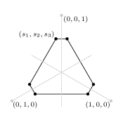
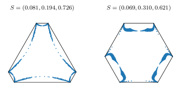
Figure 1. The unit-trace plane (left) and $\mathcal{T}^{2}(S)$ fields found numerically by randomly sampling normal directions (middle and right).

4.1.1. Lamination with $\mathcal{T}^{2}(S)$ fields

An even more informative plot can be constructed by lamination. To produce Figure 2, we first randomly generate $T\in\mathcal{T}^{2}(S)$ fields as before. Next, we draw the rank-one segment connecting $S$ to $T$, which produces a curve in the unit-trace plane. The curves appear to fill in a region with a hexagonal hole. The most interesting aspect of these plots is the outer boundary, which appears to be formed by curves passing from $S$, through a uniaxial point, and back to a different representation of $S$. Passing through a uniaxial point corresponds to an eigenvalue crossing of either the two largest or two smallest eigenvalues as we trace the rank-one curve.

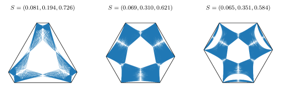
Figure 2. Rank-one curves formed by laminating $S$ with the $\mathcal{T}^{2}(S)$ fields shown in Figure 1.

Some intuition about these figures can be obtained by examining a few of the curves. Figure 3 shows some possible behaviors of these curves. The left plot shows a typical curve obtained with a random normal $n$. These rank-one curves begin at $S$, travel in the direction of a uniaxial point, but then turn back and intersect themselves without reaching a uniaxial field. Along these paths, the three eigenvalues of the lamination remain distinct.

The plot on the right shows a second type of behavior. These curves intersect one of the uniaxial lines in the plane, corresponding to a crossing of either the two smallest or two largest eigenvalues. From studying this picture, it is natural to suspect that the curves corresponding to nearly-uniaxial fields $T$ approximate the boundary curves suggested by Figure 2. From numerical experiments, eigenvalue crossings are more likely when $n_{1}n_{2}n_{3}=0$, which is consistent with Propositions 3.1 and 3.3. As stated in Remark 3.2, this condition implies that $S$, $R_{1}^{t}TR_{1}$, and $R_{2}^{t}TR_{2}$ share a common eigenvector.

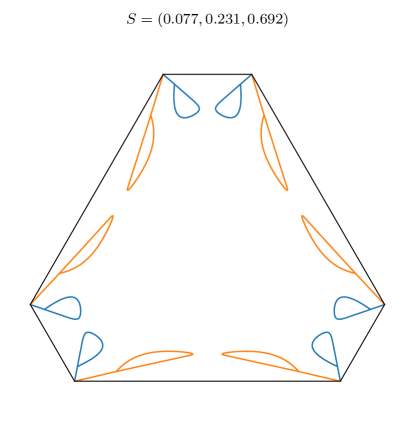
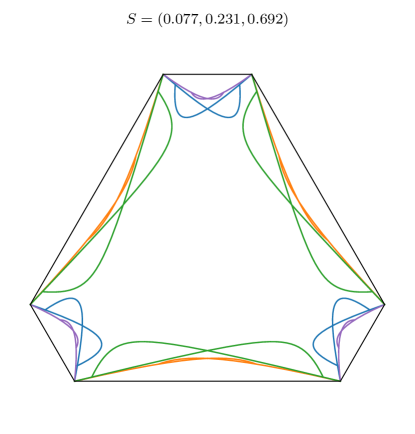
Figure 3. A few rank-one curves formed by laminating $S$ with $\mathcal{T}^{2}(S)$ fields. Those on the left do not experience an eigenvalue crossing; those on the right do.

The picture becomes clearer if we repeat the experiments of Figure 2, restricting ourselves to $n$ lying in one of the coordinate planes. The result is shown in Figure 4. The line colors in the plots indicate the coordinate plane $n$ is located in.

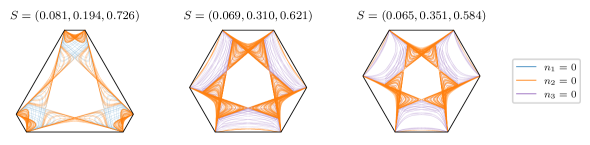
Figure 4. Rank-one curves formed by laminating $S$ with $\mathcal{T}^{2}(S)$ fields when $n$ is restricted to a coordinate plane.

From the previous figures, we make a few observations.

1. The lamination curves appear to fill a region with a hexagonal hole.

2. The hexagonal hole is expected; we know that $\mathcal{T}^{1}(S)$ fields are restricted to the exterior of a hexagon, see Figure 2.

3. The outer boundary of the region does not appear to be a laminate curve of $\mathcal{T}^{2}(S)$-type. Instead, it looks like an envelope of such curves. This is an important point. The theory developed in the rest of the paper shows that the numerical observations are exactly right. The boundary of the set is attained by a closure argument. Specifically, one shows that the uniaxial point on each of the envelope curves is attainable as a limit of attainable points. The envelope curve is then obtained as a lamination of $S$ and such uniaxial points. This is exactly the content of Section 6.

4. The $n_{2}=0$ case seems to be the important case for determining the outer boundary. For a given choice of $S$, $\mathcal{T}^{2}(S)$ fields seem to always exist with $n_{2}=0$, but may or may not exist with $n$ in one of the other coordinate planes. This set is introduced in studied in Section 5.

4.1.2. Numerically finding the envelope curves

Guided by Figure 4, we now fix $n_{2}=0$ and consider the one-parameter family of normal vectors $n=(\cos(\phi),0,\sin(\phi))^{T}$. If we define the function

$$q(\phi)=3\lambda_{0}+2n^{T}S_{n}^{-1}n,$$

then the previous analysis shows that we can find a $\mathcal{T}^{2}(S)$ fields if and only if $q(\phi)<0$. Figure 5 shows the graphs of $q(\phi)$ corresponding to the plots above.

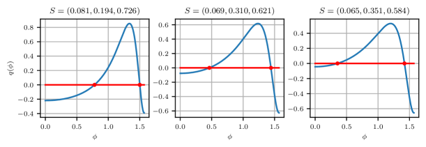
Figure 5. The function $q(\phi)$ used to find the envelope curves described in Section 4.1.2.

Notice that, in all cases, $q(\phi)$ has two zeros. One might expect that these two zeros correspond to the two uniaxial points on the outer boundary of the regions above. The intuition is as follows. If $\phi$ is such that $q(\phi)<0$ but $q(\phi)\approx 0$, then $h\approx 0$. This implies that $\lambda_{1}\approx\lambda_{2}\approx\lambda_{0}$, and, therefore, that $S(\lambda_{i})$ for $i=0,1,2$ all have nearly identical eigenvalues. However, we also know that $S(\lambda)$ has an eigenvalue crossing somewhere between $\lambda_{1}$ and $\lambda_{2}$. So, the eigenvalues cannot move very much in the interval, but they also must cross. This implies that the $S(\lambda_{i})$ are nearly uniaxial. We expect, then, that as $\phi$ approaches one of the zeros of $q$, the fields $S(\lambda_{i})$ converge to a uniaxial point. That suggests that the envelope is formed by the rank-one segment connecting $S$ to this limiting uniaxial point, as actually proved in Section 6.

To check this, we can find the roots of $q$ numerically, compute the uniaxial fields $S(\lambda_{0})$ (for the values of $\phi$ where $q(\phi)$ vanishes) and draw the rank one curves superimposed on the plots of laminate curves above. The result is shown in Figure 6. In this case, we do not use color to distinguish the plane in which $n$ lies. Instead, all laminate curves are plotted in the same gray color. Plotted together, this collection of curves approximately shades the region between an inner hexagon and some outer boundary curves described above.

The dots in the figure indicate the special uniaxial fields while the dashed curves indicate the rank-one line connecting these fields with $S$. As anticipated, these curves do appear to form the envelope of the laminates with $\mathcal{T}^{2}(S)$ fields. It is important to remember that the uniaxial points are not $\mathcal{T}^{2}(S)$ fields, but, instead, represent limits of certain $\mathcal{T}^{2}(S)$ fields.

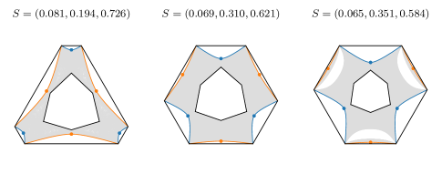
Figure 6. The gray curves are formed as in Figure 4, but removing the color coding. The orange and blue curves show the envelope found numerically using the method of Section 4.1.2. The inner hexagon shows the boundary of the set $A(T,S)=\emptyset$ given in Proposition 2.9; there are no $\mathcal{T}^{1}$ fields inside this hexagon.

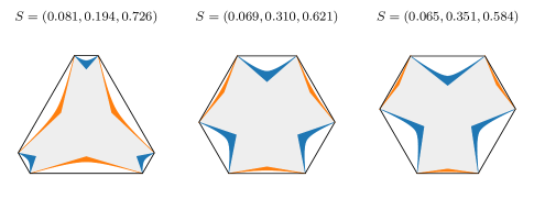
Figure 7. Comparison of Figure 6 with the constructions in [27]. The shaded gray region is formed by the procedure described in [27]. The darker shaded regions are additional fields found by the constructions in the present paper.

Next Figure 7 compares Figure 6 with the result obtained in [27]. The colored parts are the progress made. Let us comment here, that the content of the paper is two-fold. On one hand, we prove the progress, on the other hand, we prove in Section 9, roughly speaking, that no further progress can be made in the class of laminate microstructures.

5. The subset $\mathcal{T}^{2}_{2}(S)$ of ${\mathcal{T}}^{2}(S)$

In the present section, inspired by the simulations already presented, we introduce a subset of $\mathcal{T}^{2}(S)$ for which $n_{2}=0$. Before proceeding, let us digress briefly to comment about the index “two”, i.e., neither “one” nor “three”. The comment is intended for the experts on the effective behavior of conducting media, in particular to those that already know the physical context of polycrystalline conductivity which is reviewed in Section 10. The reader may wonder why focusing on the condition $n_{2}=0$ and not on the conditions $n_{1}=0$ or $n_{3}=0$. Here is a quick explanation. The index two is linked to the intermediate value $s_{2}\in(s_{1},s_{3})$. In physical terms, when one looks at the polycrystal problem that originates the differential inclusion, the laminations with $n_{2}=0$ achieve “harmonic mean” behavior along the intermediate principal conductivity, while laminations with $n_{1}=0$ or $n_{3}=0$ are related to “harmonic mean” behavior in the smallest and largest principal conductivity. Actually, they have been already used in [4] to prove optimality of different bounds for effective conductivity. Roughly speaking, they were trying to maximize effective conductivity, while in the present paper, our microgeometry maximize resistivity or, equivalently, minimize effective conductivity. However, in contrast with the problem treated in the present paper, in the case of the upper bound [4], rank-two laminates suffice.

We now define the set $\mathcal{T}^{2}_{2}(S)$. Its elements are the seed materials we will work with. Define the function $F:[s_{1},s_{3}]^{2}\to\mathbb{R}$ as

(5.1) $$F(x,y):=\left(\frac{s_{1}\,s_{3}}{s_{2}}\right)\frac{\,x\,y}{x^{2}+x\,y+y^{2}-s_{2}\,(x+y)}.$$

Definition 5.1.

Assume that $T$ has distinct eigenvalues. We say that $T\in\mathcal{T}^{2}_{2}(S)$ if $T$ satisfies either

(5.2) $$\left\{\begin{array}[]{ll}(\alpha_{-}(T,S),\alpha_{+}(T,S))=\displaystyle{\left(\frac{t_{1}}{s_{2}},\frac{t_{2}}{s_{2}}\right)}\\ \\ t_{3}=F(t_{1},t_{2})\end{array}\right.$$

or

(5.3) $$\left\{\begin{array}[]{ll}(\beta_{-}(T,S),\beta_{+}(T,S))=\displaystyle{\left(\frac{t_{2}}{s_{2}},\frac{t_{3}}{s_{2}}\right)}\\ \\ t_{1}=F(t_{3},t_{2})\end{array}\right.$$

where $F$ is given by (5.1).

Remark 5.2.

Note that

$$(\alpha_{-}(T,S),\alpha_{+}(T,S))=\displaystyle{\left(\frac{t_{1}}{s_{2}},\frac{t_{2}}{s_{2}}\right)}\Longleftrightarrow\displaystyle{\frac{t_{2}}{t_{3}}\leq\frac{s_{2}}{s_{3}}\leq\frac{t_{1}}{t_{2}}},$$

$$(\beta_{-}(T,S),\beta_{+}(T,S))=\displaystyle{\left(\frac{t_{2}}{s_{2}},\frac{t_{3}}{s_{2}}\right)}\Longleftrightarrow\frac{t_{1}}{t_{2}}\leq\frac{s_{1}}{s_{2}}\leq\frac{t_{2}}{t_{3}}.$$

Proposition 5.3.

The following holds:

$$\mathcal{T}^{2}_{2}(S)\subset{\mathcal{T}}^{2}(S).$$

Proof.

Part 1. Assume (5.2) holds. Set $(\lambda_{1},\lambda_{2})=(\alpha_{-}(T,S),\alpha_{+}(T,S))$. Choose $n_{2}=0$ and set

(5.4) $$\begin{array}[]{lll}n=\left(\begin{array}[]{c}\cos\varphi\\ 0\\ \sin\varphi\end{array}\right),&R_{1}=\left(\begin{array}[]{ccc}0&-1&0\\ -\cos\theta_{1}&0&\sin\theta_{1}\\ -\sin\theta_{1}&0&-\cos\theta_{1}\end{array}\right),&R_{2}=\left(\begin{array}[]{ccc}\cos\theta_{2}&0&-\sin\theta_{2}\\ 0&1&0\\ \sin\theta_{2}&0&\cos\theta_{2}\end{array}\right),\end{array}$$

for some suitably chosen angles $\varphi,\theta_{1},\theta_{2}$. Then we have

(5.5) $$\lambda_{1}\,S+(1-\lambda_{1})\,n\otimes n=\left(\begin{array}[]{ccc}\lambda_{1}\,s_{1}+(1-\lambda_{1})\cos^{2}\varphi&0&(1-\lambda_{1})\cos\varphi\,\sin\varphi\\ 0&\lambda_{1}\,s_{2}&0\\ (1-\lambda_{1})\cos\varphi\,\sin\varphi&0&\lambda_{1}\,s_{3}+(1-\lambda_{1})\sin^{2}\varphi\end{array}\right).$$

On the other hand,

(5.6) $$R_{1}^{t}TR_{1}=\left(\begin{array}[]{ccc}t_{2}\,\cos^{2}\theta_{1}+t_{3}\,\sin^{2}\theta_{1}&0&(t_{3}-t_{2})\,\cos\theta_{1}\,\sin\theta_{1}\\ 0&t_{1}&0\\ (t_{3}-t_{2})\,\cos\theta_{1}\,\sin\theta_{1}&0&t_{2}\,\sin^{2}\theta_{1}+t_{3}\,\cos^{2}\theta_{1}\end{array}\right).$$

Recalling that $\lambda_{1}\,s_{2}=t_{1}$, we get

(5.7) $$\lambda_{1}\,S+(1-\lambda_{1})\,n\otimes n=R_{1}^{t}TR_{1}$$

if and only if

(5.8) $$\begin{array}[]{lll}\left(\begin{array}[]{ccc}t_{2}\,\cos^{2}\theta_{1}+t_{3}\,\sin^{2}\theta_{1}&(t_{3}-t_{2})\,\cos\theta_{1}\,\sin\theta_{1}\\ (t_{3}-t_{2})\,\cos\theta_{1}\,\sin\theta_{1}&t_{2}\,\sin^{2}\theta_{1}+t_{3}\,\cos^{2}\theta_{1}\end{array}\right)=\\ \\ \left(\begin{array}[]{ccc}\lambda_{1}\,s_{1}+(1-\lambda_{1})\cos^{2}\varphi&(1-\lambda_{1})\cos\varphi\,\sin\varphi\\ (1-\lambda_{1})\cos\varphi\,\sin\varphi&\lambda_{1}\,s_{3}+(1-\lambda_{1})\sin^{2}\varphi\end{array}\right).\\ \\ \end{array}$$

The two matrices in (5.8) are symmetric and, by construction, their common trace equals $s_{1}+s_{3}$. Hence, they have the same eigenvalues if and only if their determinants are the same, i.e., if and only if

(5.9) $$\lambda_{1}^{2}s_{1}\,s_{3}+\lambda_{1}\,(1-\lambda_{1})(s_{3}\,\cos^{2}\varphi+s_{1}\,\sin^{2}\varphi)=t_{2}\,t_{3}$$

Setting

(5.10) $$z(\varphi):=s_{3}\,\cos^{2}\varphi+s_{1}\,\sin^{2}\varphi,$$

we write (5.9) as

(5.11) $$z(\varphi)=z_{1}(T,S):=\frac{t_{2}\,t_{3}-\lambda_{1}^{2}\,s_{1}\,s_{3}}{\lambda_{1}\,(1-\lambda_{1})}=\frac{s_{2}^{2}\,t_{2}\,t_{3}-s_{1}s_{3}\,t_{1}^{2}}{(s_{2}-t_{1})\,t_{1}}.$$

The same calculation for the second index yields

(5.12) $$R_{2}^{t}TR_{2}=\begin{array}[]{lll}\left(\begin{array}[]{ccc}t_{1}\,\cos^{2}\theta_{2}+t_{3}\,\sin^{2}\theta_{2}&0&(t_{3}-t_{1})\,\cos\theta_{2}\,\sin\theta_{2}\\ 0&t_{2}&0\\ (t_{3}-t_{1})\,\cos\theta_{2}\,\sin\theta_{2}&0&t_{3}\,\cos^{2}\theta_{2}+t_{1}\,\sin^{2}\theta_{2}\end{array}\right),\end{array}$$

and recalling that $\lambda_{2}\,s_{2}=t_{2}$, we get

(5.13) $$\lambda_{2}\,S+(1-\lambda_{2})\,n\otimes n=R_{2}^{t}TR_{2}$$

if and only if

$$\begin{array}[]{lll}\left(\begin{array}[]{ccc}t_{1}\,\cos^{2}\theta_{2}+t_{3}\,\sin^{2}\theta_{2}&(t_{3}-t_{1})\,\cos\theta_{2}\,\sin\theta_{2}\\ (t_{3}-t_{1})\,\cos\theta_{2}\,\sin\theta_{2}&t_{1}\,\sin^{2}\theta_{2}+t_{3}\,\cos^{2}\theta_{2}\end{array}\right)=\\ \\ \left(\begin{array}[]{ccc}\lambda_{2}\,s_{1}+(1-\lambda_{2})\cos^{2}\varphi&(1-\lambda_{2})\cos\varphi\,\sin\varphi\\ (1-\lambda_{2})\cos\varphi\,\sin\varphi&\lambda_{2}\,s_{3}+(1-\lambda_{2})\sin^{2}\varphi\end{array}\right).\end{array}$$

As in the previous calculation, we deduce that they share the same eigenvalues if and only if

$$\lambda_{2}^{2}s_{1}\,s_{3}+\lambda_{2}\,(1-\lambda_{2})(s_{3}\,\cos^{2}\varphi+s_{1}\,\sin^{2}\varphi)=t_{1}\,t_{3}\,.$$

Recalling (5.10), the previous equation requires

(5.14) $$z(\varphi)=z_{2}(T,S):=\frac{t_{1}\,t_{3}-\lambda_{2}^{2}\,s_{1}\,s_{3}}{\lambda_{2}\,(1-\lambda_{2})}=\frac{s_{2}^{2}\,t_{1}\,t_{3}-s_{1}s_{3}\,t_{2}^{2}}{(s_{2}-t_{2})\,t_{2}}.$$

The pair $(T,S)$ satisfies

$$z_{1}(T,S)=z_{2}(T,S)$$

if and only if

(5.15) $$\frac{s_{2}^{2}\,t_{2}\,t_{3}-s_{1}s_{3}\,t_{1}^{2}}{(s_{2}-t_{1})\,t_{1}}=\frac{s_{2}^{2}\,t_{1}\,t_{3}-s_{1}\,s_{3}\,t_{2}^{2}}{t_{2}(s_{2}-t_{2})}.$$

One can check that if (5.15) holds, then the common value $z(\varphi)\in[s_{1},s_{3}]$. On the other hand, by choosing $\varphi$ appropriately, by the Definition 5.10, $z(\varphi)$ may assume any value belonging to $[s_{1},s_{3}]$. Since (5.15) is equivalent to the second condition in (5.2), we conclude that if the pair $(T,S)$ satisfies (5.2), then (4.1) holds, thus ending the proof of Part 1.

Part 2. Assume (5.3) holds. Set $(\lambda_{2},\lambda_{1})=(\beta_{-}(T,S),\beta_{+}(T,S))$. Choose again $n_{2}=0$ and set

(5.16) $$\begin{array}[]{lll}n=\left(\begin{array}[]{c}\cos\psi\\ 0\\ \sin\psi\end{array}\right),&R_{1}=\left(\begin{array}[]{ccc}\cos\gamma_{1}&0&-\sin\gamma_{1}\\ \sin\gamma_{1}&0&\cos\gamma_{1}\\ 0&-1&0\end{array}\right),&R_{2}=\left(\begin{array}[]{ccc}\cos\gamma_{2}&0&-\sin\gamma_{2}\\ 0&1&0\\ \sin\gamma_{2}&0&\cos\gamma_{2}\end{array}\right),\end{array}$$

for some suitably chosen angles $\psi,\gamma_{1},\gamma_{2}$. Then we have

(5.17) $$\lambda_{1}\,S+(1-\lambda_{1})\,n\otimes n=\left(\begin{array}[]{ccc}\lambda_{1}\,s_{1}+(1-\lambda_{1})\cos^{2}\psi&0&(1-\lambda_{2})\cos\psi\,\sin\psi\\ 0&\lambda_{1}\,s_{2}&0\\ (1-\lambda_{2})\cos\psi\,\sin\psi&0&\lambda_{2}\,s_{3}+(1-\lambda_{2})\sin^{2}\psi\end{array}\right).$$

On the other hand

(5.18) $$R_{1}^{t}TR_{1}=\left(\begin{array}[]{ccc}t_{1}\,\cos^{2}\gamma_{1}+t_{2}\,\sin^{2}\gamma_{1}&0&(t_{2}-t_{1})\,\cos\gamma_{1}\,\sin\gamma_{1}\\ 0&t_{3}&0\\ (t_{2}-t_{1})\,\cos\gamma_{1}\,\sin\gamma_{1}&0&t_{1}\,\sin^{2}\gamma_{1}+t_{2}\,\cos^{2}\gamma_{2}\\ \end{array}\right).$$

Recalling that $\lambda_{1}\,s_{2}=t_{3}$, we get

(5.19) $$\lambda_{1}\,S+(1-\lambda_{1})\,n\otimes n=R_{1}^{t}TR_{1}$$

if and only if

(5.20) $$\begin{array}[]{lll}\left(\begin{array}[]{ccc}t_{1}\,\cos^{2}\gamma_{1}+t_{2}\,\sin^{2}\gamma_{1}&(t_{2}-t_{1})\,\cos\gamma_{1}\,\sin\gamma_{1}\\ (t_{2}-t_{1})\,\cos\gamma_{1}\,\sin\gamma_{1}&t_{2}\,\sin^{2}\gamma_{1}+t_{1}\,\cos^{2}\gamma_{1}\end{array}\right)=\\ \\ \left(\begin{array}[]{ccc}\lambda_{1}\,s_{1}+(1-\lambda_{1})\cos^{2}\psi&(1-\lambda_{1})\cos\psi\,\sin\psi\\ (1-\lambda_{1})\cos\psi\,\sin\psi&\lambda_{1}\,s_{3}+(1-\lambda_{1})\sin^{2}\psi\end{array}\right).\\ \\ \end{array}$$

The two matrices in (5.20) are symmetric and, by construction, their common trace equals $s_{1}+s_{3}$. Hence, they have the same eigenvalues if and only if their determinants are the same, i.e., if and only if

(5.21) $$\lambda_{1}^{2}s_{1}\,s_{3}+\lambda_{1}\,(1-\lambda_{1})(s_{3}\,\cos^{2}\psi+s_{1}\,\sin^{2}\psi)=t_{1}\,t_{2}.$$

Setting

(5.22) $$z(\psi):=s_{3}\,\cos^{2}\psi+s_{1}\,\sin^{2}\psi,$$

we write (5.21) as

(5.23) $$z(\psi)=z_{3}(T,S):=\frac{t_{2}\,t_{1}-\lambda_{1}^{2}\,s_{1}\,s_{3}}{\lambda_{1}\,(1-\lambda_{1})}=\frac{s_{2}^{2}\,t_{2}\,t_{1}-s_{1}s_{3}\,t_{3}^{2}}{(s_{2}-t_{3})\,t_{3}}.$$

As in the calculation for Part 1, we deduce that they share the same eigenvalues if and only if

$$\lambda_{2}^{2}s_{1}\,s_{3}+\lambda_{2}\,(1-\lambda_{2})(s_{3}\,\cos^{2}\psi+s_{1}\,\sin^{2}\psi)=t_{1}\,t_{3}\,.$$

Now we proceed with the same calculation for the second index

(5.24) $$R_{2}^{t}TR_{2}=\begin{array}[]{lll}\left(\begin{array}[]{ccc}t_{1}\,\cos^{2}\gamma_{2}+t_{3}\,\sin^{2}\gamma_{2}&0&(t_{3}-t_{1})\,\cos\gamma_{2}\,\sin\gamma_{2}\\ 0&t_{2}&0\\ (t_{3}-t_{1})\,\cos\gamma_{2}\,\sin\gamma_{2}&0&t_{3}\,\cos^{2}\gamma_{2}+t_{1}\,\sin^{2}\gamma_{2}\end{array}\right).\end{array}$$

Recalling that $\lambda_{2}\,s_{2}=t_{2}$, we get

(5.25) $$\lambda_{2}\,S+(1-\lambda_{2})\,n\otimes n=R_{2}^{t}TR_{2}$$

if and only if

(5.26) $$\begin{array}[]{lll}\left(\begin{array}[]{ccc}t_{1}\,\cos^{2}\gamma_{2}+t_{3}\,\sin^{2}\gamma_{2}&(t_{3}-t_{1})\,\cos\gamma_{2}\,\sin\gamma_{2}\\ (t_{3}-t_{1})\,\cos\gamma_{2}\,\sin\gamma_{2}&t_{1}\,\sin^{2}\gamma_{2}+t_{3}\,\cos^{2}\gamma_{2}\end{array}\right)=\\ \\ \left(\begin{array}[]{ccc}\lambda_{2}\,s_{1}+(1-\lambda_{2})\cos^{2}\psi&(1-\lambda_{2})\cos\psi\,\sin\psi\\ (1-\lambda_{2})\cos\psi\,\sin\psi&\lambda_{2}\,s_{3}+(1-\lambda_{2})\sin^{2}\psi\end{array}\right).\end{array}$$

Proceeding as in Part 1, the two matrices have the same eigenvalues if and only if

(5.27) $$\lambda_{2}^{2}s_{1}\,s_{3}+\lambda_{2}\,(1-\lambda_{2})(s_{3}\,\cos^{2}\psi+s_{1}\,\sin^{2}\psi)=t_{1}\,t_{3}\,.$$

Recalling (5.22) we write the previous equation as

(5.28) $$z(\psi)=z_{4}(T,S):=\frac{t_{1}\,t_{3}-\lambda_{2}^{2}\,s_{1}\,s_{3}}{\lambda_{2}\,(1-\lambda_{2})}=\frac{s_{2}^{2}\,t_{1}\,t_{3}-s_{1}s_{3}\,t_{2}^{2}}{(s_{2}-t_{2})\,t_{2}}.$$

The pair $(T,S)$ satisfies

$$z_{3}(T,S)=z_{4}(T,S)$$

if and only if

(5.29) $$\frac{s_{2}^{2}\,t_{1}\,t_{2}-s_{1}s_{3}\,t_{3}^{2}}{(s_{2}-t_{3})\,t_{3}}=\frac{s_{2}^{2}\,t_{1}\,t_{3}-s_{1}\,s_{3}\,t_{2}^{2}}{t_{2}(s_{2}-t_{2})}.$$

One can check that if (5.29) holds, then the common value $z(\psi)\in[s_{1},s_{3}]$. On the other hand, by choosing $\psi$ appropriately, by the definition (5.22), $z(\psi)$ may assume any value belonging to $[s_{1},s_{3}]$. Since (5.29) is equivalent to the second condition in(5.3), we conclude that if the pair $(T,S)$ satisfies (5.3), then (4.1) holds, thus ending the proof of Part 2. ∎

6. Explicit analytic description of the new optimal set $\mathcal{L}$

The goal of the present section is to prove Proposition 6.6, which characterizes the set $\mathcal{L}$, whose definition is given in Definition 6.4.

Definition 6.1.

Set

(6.1) $$\begin{array}[]{cc}U_{-}=\left(\begin{array}[]{ccc}u_{-}&0&0\\ 0&u_{-}&0\\ 0&0&1-2u_{-}\end{array}\right),\quad U_{+}=\left(\begin{array}[]{ccc}1-2u_{+}&0&0\\ 0&u_{+}&0\\ 0&0&u_{+}\end{array}\right),\end{array}$$

where $u_{-}$ and $u_{+}$ are the smallest and greatest roots of

(6.2) $$h(x)=0,\quad h(x):=6s_{2}\,x^{2}+x\,(s_{1}s_{3}-3s_{2}-4s_{2}^{2})+2s_{2}^{2}$$

respectively. Set

(6.3) $$\begin{array}[]{ccc}n_{\pm}=\left(\begin{array}[]{c}\cos\varphi_{\pm}\\ 0\\ \sin\varphi_{\pm}\end{array}\right),\,R_{-}=\left(\begin{array}[]{ccc}0&-1&0\\ -\cos\theta_{-}&0&\sin\theta_{-}\\ -\sin\theta_{-}&0&-\cos\theta_{-}\end{array}\right),\,R_{+}=\left(\begin{array}[]{ccc}\cos\theta_{+}&0&-\sin\theta_{+}\\ \sin\theta_{+}&0&\cos\theta_{+}\\ 0&-1&0\end{array}\right),\end{array}$$

with

(6.4) $$\cos(2\varphi_{\pm})=\frac{s_{2}(s_{1}+s_{3})+u_{\pm}(2s_{1}s_{3}-s_{1}-s_{3})}{(s_{3}-s_{1})(s_{2}-u_{\pm})},$$

and

(6.5) $$\begin{array}[]{ll}\displaystyle{\cos(2\theta_{\pm})=\mp\frac{u_{\pm}(s_{3}-s_{1})+(u_{\pm}-s_{2})\cos(2\varphi_{\pm})}{s_{2}(1-3u_{\pm})}.}\end{array}$$

The matrices $U^{-}$ and $U^{+}$ correspond to the blue and orange points in Figures 6 and 7. In order to define $\mathcal{L}$, we define two curves in eigenvalue space, which we call $\Gamma_{\pm}$. We will need an efficient way to describe such curves. Let $F,G\in K^{*}(S)$ and assume that the set $A(G,F)$ has non-empty interior and

$$R^{t}GR=\lambda F+(1-\lambda)n(\lambda)\otimes n(\lambda),\quad\lambda\in A(G,F).$$

For a given $\lambda\in A(G,F)$ we consider the one-parameter family of matrices

$$\begin{array}[]{l}\widehat{M}(\lambda,t)=t(\lambda F+(1-\lambda)n(\lambda)\otimes n(\lambda))+(1-t)\lambda F=\\ \\ \lambda\,F+t(1-\lambda)n(\lambda)\otimes n(\lambda),\quad t\in[0,1].\end{array}$$

Now normalize to trace one by setting

(6.6) $$\begin{array}[]{l}\displaystyle{M(\lambda,t)=\frac{\widehat{M}(\lambda,t)}{{\rm Tr}\widehat{M}(\lambda,t)}=\eta(\lambda,t)F+(1-\eta(\lambda,t))n(\lambda)\otimes n(\lambda),\quad\eta(\lambda,t):=\frac{\lambda}{\lambda+t(1-\lambda)}},\end{array}$$

and note that

$$M(\lambda,0)=F,\quad M(\lambda,1)=R^{t}GR.$$

Denote by

(6.7) $$m_{1}(\lambda,t)\leq m_{2}(\lambda,t)\leq m_{3}(\lambda,t)$$

the eigenvalues of $M(\lambda,t)$. We now specialize (6.6) to the case when $F=S$ and $G=U^{\pm}$. Consider the families of matrices

(6.8) $$\begin{array}[]{l}\displaystyle{F_{-}(t):=M(\alpha_{-},t)=\eta(\alpha_{-},t)S+(1-\eta(\alpha_{-},t))n^{-}\otimes n^{-}},\quad\alpha_{-}:=\alpha_{-}(U_{-},S)=\frac{u_{-}}{s_{2}},\\ \\ \displaystyle{F_{+}(t):=M(\beta_{+},t)=\eta(\beta_{+},t)S+(1-\eta(\beta_{+},t))n^{+}\otimes n^{+}},\quad\beta_{+}:=\beta_{+}(U_{+},S)=\frac{u_{+}}{s_{2}}.\end{array}$$

Definition 6.2.

The curves $\Gamma_{\pm}$ are defined as follows. Consider the parametric curves (6.7) associated to (6.8):

(6.9) $$t\to m(\alpha_{-},t):=(m_{1}(\alpha_{-},t),m_{2}(\alpha_{-},t),m_{3}(\alpha_{-},t)),\quad t\in[0,1]$$

(6.10) $$t\to m(\beta_{+},t):=(m_{1}(\beta_{+},t),m_{2}(\beta_{+},t),m_{3}(\beta_{+},t)),\quad t\in[0,1].$$

Then

$$\Gamma_{-}:=m(\alpha_{-},[0,1]),\quad\Gamma_{+}:=m(\beta_{+},[0,1]).$$

The curves $\Gamma_{\pm}$ are shown in Figure 8(a).

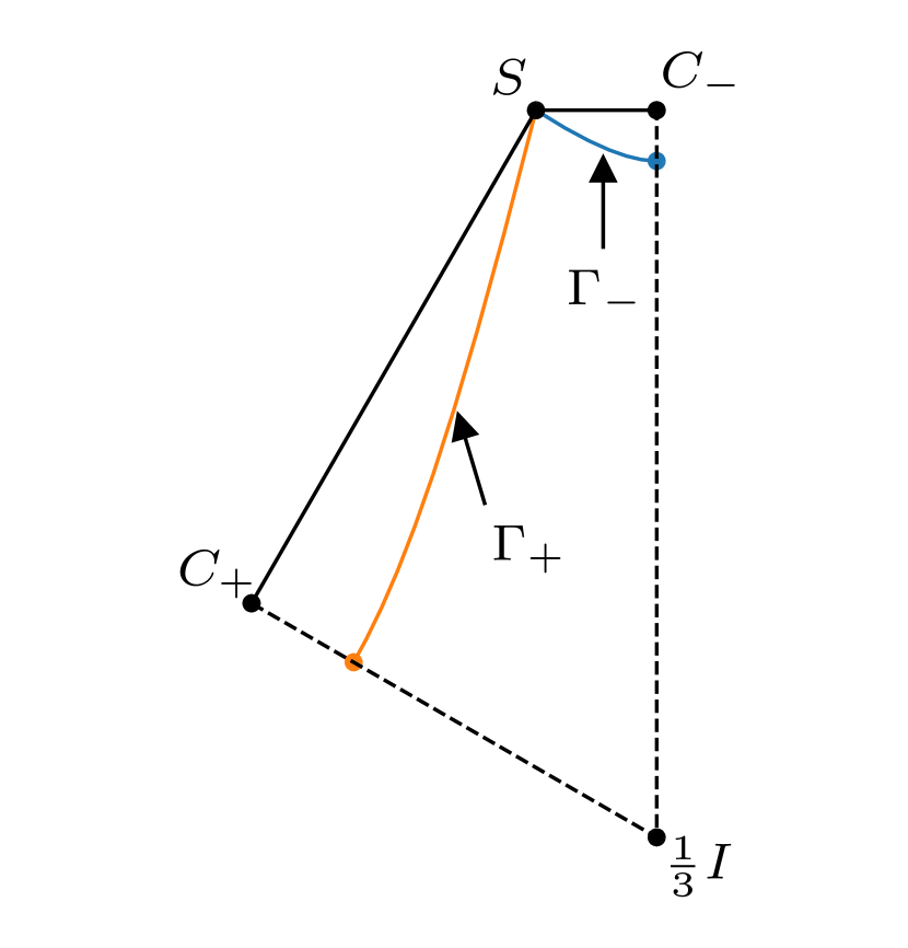
(a)

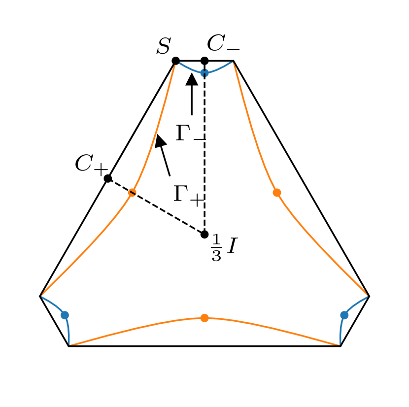
(b)

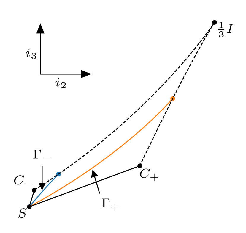
(c)

Figure 8. The left figure shows important fields in one sextant ($s_{1}\leq s_{2}\leq s_{3}$) of the unit-trace plane. The outer quadrilateral connects the field $S$ to the isotropic field $\frac{1}{3}I$ and the two uni-axial points, $C_{-}=(\frac{s_{1}+s_{2}}{2},\frac{s_{1}+s_{2}}{2},s_{3})$ and $C_{+}=(s_{1},\frac{s_{2}+s_{3}}{2},\frac{s_{2}+s_{3}}{2})$. The curves $\Gamma_{-}$ and $\Gamma_{+}$ from Definition 6.2 are also shown, together with their intersections with the uniaxial lines. The center figure shows the construction in Definition 6.3. The set $\mathcal{L}$ is enclosed by the union of the reflected copies of $\Gamma_{\pm}$. The rightmost figure shows the fields in the sextant once again, but in the plane of the matrix invariants, $(i_{2},i_{3})$, which are used in the stability proof of Section 8.

Definition 6.3.

The closed curve $\Gamma$ is obtained as follows. First, reflect $\Gamma_{-}$ along the line $m_{1}=m_{2}$ in the plane $m_{1}+m_{2}+m_{3}=1$, then consider the union of the curves obtained with its $2\pi/3$ rotations within the unit trace plane. Next, reflect $\Gamma_{+}$ along the line $m_{2}=m_{3}$ in the plane $m_{1}+m_{2}+m_{3}=1$, and consider the union of the curves obtained with its $2\pi/3$ rotations within the unit trace plane. Finally, $\Gamma$ is the union of the six curves thus defined.

The construction of $\Gamma$ is shown in Figure 8(b). We note that $\Gamma$ is a simple closed Jordan curve, by construction and, for future reference, that by construction we have

(6.11) $$m_{2}(\alpha_{-},t)=s_{2}\eta(\alpha_{-},t),\quad m_{2}(\beta_{+},t)=s_{2}\eta(\beta_{+},t)$$

Definition 6.4.

We denote by $\mathcal{L}$ the bounded closed set enclosed by $\Gamma$.

Remark 6.5.

Note that $\mathcal{L}$ is the union of six sets. Each one is obtained from the other by an appropriate permutation of the eigenvalues $m_{j}$. In Figure 6 the boundary of $\mathcal{L}$ is the union of the three orange and the three blue curves. In Figure 7 the set $\mathcal{L}$ is compared with the sets that were known to be attained prior to the present work.

Proposition 6.6.

Let $U_{\pm}$ be defined by (6.1). Then

• $s_{1}\leq u_{-}<\frac{1}{3}<u_{+}\leq s_{3}$.
  

• For a given $S$, the matrices $U_{\pm}$ are the unique solutions $T$ to (2.2), i.e.

  (6.12) $$R_{-}^{t}U_{-}R_{-}=\alpha_{-}S+(1-\alpha_{-})\,n_{-}\otimes n_{-},\quad\lambda_{1}=\lambda_{2}=\alpha_{-}=\alpha_{+}=\frac{u_{-}}{s_{2}},$$

  (6.13) $$R_{+}^{t}U_{+}R_{+}=\beta_{+}S+(1-\beta_{+})\,n_{+}\otimes n_{+},\quad\lambda_{2}=\lambda_{1}=\beta_{+}=\beta_{-}=\frac{u_{+}}{s_{2}},$$

  with $n_{\pm}$ and $R_{\pm}$ defined in (6.3), (6.4), and (6.5) and obtained by Lemma 2.5 in the limiting case where $t_{1}=t_{2}$ and $t_{2}=t_{3}$ respectively.
  

• The set $\mathcal{L}$ of Definition 6.4 satisfies $\mathcal{L}\subset K^{*}(S)$.
  

Proof.

(i) We have

$$h(0)=2s_{2}^{2}>0,\quad h(1)=(3-2s_{2})s_{2}+s_{1}s_{3}>0,\quad h\left(\frac{1}{3}\right)=-\frac{1}{3}(s_{1}-s_{2})(s_{2}-s_{3})<0.$$

Therefore, the two roots of $h(x)=0$ satisfy $u_{-}<1/3<u_{+}$. The other two inequalities follow from (2.1).

(ii) This follows directly from the calculations of Proposition 5.3.

(iii) This is proved in Section 7, see in particular Corollary 7.3.

∎

7. Solution to the underlying differential inclusion

In the present section, we prove that if $T\in{\mathcal{T}}^{2}(S)$, then all points that lie on the trajectories associated with (4.1) belong to $K^{*}(S)$. We do so by exhibiting an infinite rank laminate that generally uses an infinite set of rotations $R\in SO(3)$, and thus infinitely many rank-one directions of lamination. This feature seems new. In the sequel we will use the notions of laminate and splitting of a laminate, whose definitions are recalled in the Appendix A (see in particular Definition A.1). For $A,B\in\mathbb{M}^{3\times 3}$, we denote by $(A,B)$ the open segment connecting $A$ and $B$.

Theorem 7.1.

Let $T\in{\mathcal{T}}^{2}(S)$ and let $A\in(\lambda_{1}S,R_{1}^{t}TR_{1})$. There exists a sequence of laminates of finite order $\nu_{k}\in\mathcal{L}(\mathbb{M}^{3\times 3})$ such that

1. $\bar{\nu}_{k}=A$   $\forall\ k\in\mathbb{N}$;

2. $\nu_{k}(\mathbb{M}^{3\times 3}\setminus K)\to 0$  $k\to+\infty$;

3. $\int_{\mathbb{M}^{3\times 3}}|F|^{2}\ d\nu_{k}(F)<C$.

Proof.

We construct the sequence $\nu_{k}$ by successive splitting. By assumption, we have

(7.1) $$\left\{\begin{array}[]{lcc}R_{1}^{t}TR_{1}=\lambda_{1}\,S+(1-\lambda_{1})\,n\otimes n\\ \\ R_{2}^{t}TR_{2}=\lambda_{2}\,S+(1-\lambda_{2})\,n\otimes n.\end{array}\right.$$

Since $A\in(\lambda_{1}S,R_{1}^{t}TR_{1})$, there exists $p\in(0,1)$ such that $A=p\lambda_{1}S+(1-p)R_{1}^{t}TR_{1}$. We define the first laminate of the sequence as $\nu_{1}:=p\delta_{\lambda_{1}S}+(1-p)\delta_{R_{1}^{t}TR_{1}}$. The next step is to replace $\delta_{R_{1}^{t}TR_{1}}$ by the sum of two Dirac masses supported in rank-one connected matrices. For this purpose let

(7.2) $$q:=\frac{\lambda_{1}(1-\lambda_{2})}{\lambda_{2}(1-\lambda_{1})},\quad\lambda:=\frac{\lambda_{2}}{\lambda_{1}},$$

and notice that, since either $0<\lambda_{1}<\lambda_{2}<1$ or $1<\lambda_{2}<\lambda_{1}$ (see Remark 4.2), one has that $q\in(0,1)$ with $\lambda>1$ in the first case, and $\lambda<1$ in the second case. Moreover, by (7.1)

(7.3) $$\frac{1}{\lambda}R_{2}^{t}TR_{2}=\lambda_{1}S+q(1-\lambda_{1})n\otimes n.$$

Let us define

(7.4) $$\left\{\begin{array}[]{llll}S_{0}=\lambda_{1}S,&T_{0}=R_{1}^{t}TR_{1},&Q=R_{2}^{t}R_{,}\\ \\ S_{1}=\lambda Q^{t}S_{0}Q,&T_{1}=\lambda Q^{t}T_{0}Q,&M=(1-q)S_{1}+qT_{1}.\\ \end{array}\right.$$

In view of (7.4) we can write $\nu_{0}=p\delta_{S_{0}}+(1-p)\delta_{T_{0}}$. To perform the first splitting we check that $M=T_{0}$ and replace $\delta_{T_{0}}$ by $(1-q)\delta_{S_{1}}+q\delta_{T_{1}}$. By the first equation in (7.1), we have

$$T_{0}=S_{0}+(1-\lambda_{1})n\otimes n.$$

Using (7.4), we have

(7.5) $$\begin{array}[]{cccc}M=\lambda Q^{t}[(1-q)S_{0}+qT_{0}]Q=\lambda Q^{t}[(1-q)S_{0}+qS_{0}+q(1-\lambda_{1})n\otimes n]Q=\\ \\ \lambda Q^{t}[S_{0}+q(1-\lambda_{1})n\otimes n]Q=\lambda Q^{t}[\lambda_{1}S+q(1-\lambda_{1})n\otimes n]Q.\end{array}$$

Now we use (7.3) and the previous equation and get

(7.6) $$QMQ^{t}=\lambda[\lambda_{1}S+q(1-\lambda_{1})n\otimes n]=R_{2}^{t}TR_{2}.$$

Therefore, we have

(7.7) $$M=T_{0}=R_{1}^{t}TR_{1}\Longleftrightarrow QT_{0}Q^{t}=R_{2}^{t}TR_{2}\Longleftrightarrow QR_{1}^{t}TR_{1}Q^{t}=R_{2}^{t}TR_{2}\Longleftrightarrow R_{2}QR_{1}^{t}=I.$$

The latter follows from the definition of $Q$. We can now define the second laminate as

$$\nu_{1}:=p\delta_{S_{0}}+(1-p)[(1-q)\delta_{S_{1}}+q\delta_{T_{1}}].$$

Notice that $\operatorname{spt}(\nu_{1})\in K\cup\{T_{1}\}$. To iterate the above procedure, we introduce the following sequences:

(7.8) $$S_{k}:=\lambda^{k}(Q^{k})^{t}S_{0}Q^{k},\quad T_{k}:=\lambda^{k}(Q^{k})^{t}T_{0}Q^{k}.$$

We note that for each $k$ the pair $(T_{k},S_{k})$ is rank-one connected. Indeed,

(7.9) $$T_{k}-S_{k}=\lambda^{k}(Q^{k})^{t}(S_{0}-T_{0})Q^{k}=\lambda^{k}(1-\lambda_{1})(Q^{k})^{t}n\otimes nQ^{k}.$$

Moreover, for each $k$,

(7.10) $$T_{k}=(1-q)S_{k+1}+qT_{k+1}.$$

We prove (7.10) by induction. The case $k=0$ has been proved in the previous part. So assume

(7.11) $$T_{k-1}=(1-q)S_{k}+qT_{k},$$

and prove that

(7.12) $$T_{k}=(1-q)S_{k+1}+qT_{k+1}.$$

We start computing the right-hand side

(7.13) $$\begin{array}[]{l}(1-q)S_{k+1}+qT_{k+1}=\lambda^{k+1}(Q^{k+1})^{t}[(1-q)S_{0}+qT_{0}]Q^{k+1}=\\ \\ \lambda^{k+1}(Q^{k+1})^{t}[(1-q)S_{0}+qS_{0}+q(1-\lambda_{1})n\otimes n]Q^{k+1}=\lambda^{k+1}(Q^{k+1})^{t}[S_{0}+q(1-\lambda_{1})n\otimes n]Q^{k+1}=\\ \\ \lambda^{k+1}(Q^{k+1})^{t}[\lambda_{1}S+q(1-\lambda_{1})n\otimes n]Q^{k+1}.\end{array}$$

We now use (7.3) and get

$$(1-q)S_{k+1}+qT_{k+1}=\lambda^{k+1}(Q^{k+1})^{t}\left[\frac{1}{\lambda}R_{2}^{t}TR_{2}\right]Q^{k+1}.$$

To prove (7.12), we are left with proving that

(7.14) $$T_{k}=\lambda^{k+1}(Q^{k+1})^{t}\left[\frac{1}{\lambda}R_{2}^{t}TR_{2}\right]Q^{k+1},$$

namely that

(7.15) $$\lambda^{k}(Q^{k})^{t}T_{0}Q^{k}=\lambda^{k}(Q^{k+1})^{t}R_{2}^{t}TR_{2}Q^{k+1}.$$

The latter is equivalent to

(7.16) $$T_{0}=Q^{t}R_{2}^{t}TR_{2}Q\Longleftrightarrow R_{1}^{t}TR_{1}=Q^{t}R_{2}^{t}TR_{2}Q\Longleftrightarrow R_{1}^{t}=Q^{t}R_{2}^{t}\Longleftrightarrow Q=R_{2}^{t}R_{1}.$$

We can now define the sequence $\nu_{k}$ recursively. In order to obtain the laminate $\nu_{k+1}$ from $\nu_{k}$, we use (7.9) and (7.12) to replace $\delta_{T_{k}}$ in $\nu_{k}$ by $(1-q)\delta_{S_{k+1}}+q\delta_{T_{k+1}}$. By construction each $\nu_{k}$ has barycenter $A$ and satisfies

$$\operatorname{spt}(\nu_{k})\subset K\cup\{T_{k}\},\quad\nu_{k}(T_{k})=(1-p)q^{k}\to 0\quad k\to 0.$$

It remains to check that (iii) holds. We explicitly compute

$$\int_{\mathbb{R}^{3\times 3}}|F|^{2}\ d\nu_{k+1}(F) =p|S_{0}|^{2}+(1-p)(1-q)\sum_{j=0}^{k}q^{j}|S_{j+1}|^{2}$$

$$=p|S_{0}|^{2}+(1-p)(1-q)|S_{0}|^{2}\lambda_{1}^{2}\lambda^{2}\sum_{j=0}^{k}(q\lambda)^{2}.$$

Since $q\lambda<1$ in each of the two cases, one has that ${\displaystyle\sup_{k}\int_{\mathbb{R}^{3\times 3}}|F|^{2}\ d\nu_{k}(F)<C}$. ∎

Corollary 7.2.

If $T\in{\mathcal{T}}^{2}(S)$, then for each $A\in[\lambda_{1}S,R_{1}^{t}TR_{1}]$ there exists $R\in SO(3)$ such that the matrix ${\displaystyle\frac{1}{\operatorname{Tr}A}R^{t}AR}$ belongs to $K^{*}(S)$. In particular $\partial\mathcal{L}\subset K^{*}$.

Proof.

The proof is a consequence of Theorem 7.1 and Proposition A.2. ∎

Corollary 7.3.

$\mathcal{L}\subset K^{*}(S)$.

Proof.

This is a consequence of Corollary 7.2 and the fact that each point in the interior of $\mathcal{L}$ belongs to a rank-one segment connecting two points of $K^{*}$. Indeed, in [27], the authors prove what they call the straight-line attainability property. In our context, this means the following. Suppose the pair $F^{*}$ and $G^{*}$ have positive eigenvalues and unitary trace and that, for some $s^{*}\in(0,1)$ they both lie on the line $t\to(ts^{*},t(1-s^{*}),1-t)$ (or any of the cyclic permutation of it) and that they belong to $K^{*}(S)$, then the entire segment joining $F^{*}$ and $G^{*}$ does. Indeed one can find $\lambda\in\mathbb{R}$ such that $F^{*}$ and $\lambda G^{*}$ are rank-one connected along the direction $(0,0,1)\otimes(0,0,1)$.

∎

8. A characterization of the stability under lamination of the set $\mathcal{L}$

In this section, we first define analytically the stability under lamination of a set. Then, in Proposition 8.4, we provide an equivalent description in terms of geometrical quantities. Finally, we state Proposition 8.14, proved in the following section, which implies stability.

Definition 8.1.

We say that a subset $L$ of $K^{*}(S)$ is stable under lamination if the following holds. For any pair $F,G\in L$ such that $\operatorname{rank}(\lambda F-R^{t}GR$) =1 for some $\lambda\in\mathbb{R}$ and $R\in SO(3)$, the projection on $K^{*}(S)$ of the rank-one segment connecting $\lambda F$ and $R^{t}GR$ belongs to $L$. Namely, if $t\to M(\lambda,t)$ is the curve defined by (6.6), then the curve $t\to m(\lambda,t)=(m_{1}(\lambda,t),m_{2}(\lambda,t),m_{3}(\lambda,t))$ of corresponding eigenvalues, satisfies $m(\lambda,t)\in L$ for each $t\in[0,1]$.

Remark 8.2.

It is well-known that the set $K^{*}$ is closed under lamination.

The most natural variables in our problem are the symmetric invariants, rather than the eigenvalues. The change of variable is a diffeomorphism, except at points where two eigenvalues collapse. As we will see, this will cause no harm (see Remark 8.16). For this reason, we now describe the set $\mathcal{L}$ in the space of symmetric invariants as follows. Set

(8.1) $$x(\lambda,t):=i_{2}(M(\lambda,t)),\quad y(\lambda,t):=i_{3}(M(\lambda,t)),\quad\dot{x}(\lambda,t)=\frac{\partial x}{\partial t}(\lambda,t),\quad\dot{y}(\lambda,t)=\frac{\partial y}{\partial t}(\lambda,t),$$

and,

(8.2) $$x_{F}:=x(\lambda,0),\quad x_{G}:=x(\lambda,1),\quad y_{F}:=y(\lambda,0),\quad y_{G}:=y(\lambda,1).$$

See Figure 8(c) for plot of important fields in these coordinates. The curves $\Gamma_{\pm}$ will be denoted by $\gamma_{\pm}$ in the $(x,y)$-space, as clarified by the following definition.

Definition 8.3.

The curve $\gamma_{\pm}$ are defined as follows. For $F_{\pm}$ given by (6.8) and $t\in[0,1]$, set

$$\Phi_{-}(t):=(i_{2}(F_{-}(t)),i_{3}(F_{-}(t))),\quad\Phi_{+}(t):=(i_{2}(F_{+}(t)),i_{3}(F_{+}(t))).$$

Then

(8.3) $$\gamma_{\pm}:=\Phi_{\pm}([0,1]).$$

Abusing notation, we identify points in matrix space with points in invariant space, so we can write $F_{\pm}(t)\in\gamma_{\pm}$. Note that $F_{\pm}(0)=S$ and $F_{\pm}(1)=U_{\pm}$.

Proposition 8.4.

The set $\mathcal{L}$ given by Definition 6.4 is stable under lamination if and only if the following geometrical property holds. Let $F_{1},F_{2}$ both belong to either $\gamma_{-}$ or $\gamma_{+}$, with $F_{1}$ the closest to $S$. Then the tangent vector at $F_{1}$ to any rank-one trajectory joining $F_{1}$ and $F_{2}$, points strictly inwards $\mathcal{L}$, except for the optimal rank-one trajectory which lies exactly on $\partial\mathcal{L}$.

Proof.

The condition is clearly necessary. We focus on the sufficiency. Let $F,G\in\mathcal{L}$ be such that $\operatorname{rank}(\lambda F-R^{t}GR)=1$ for some $\lambda\in\mathbb{R}$ and $R\in SO(3)$. Let $m(\lambda,t)$ be as in Definition 8.1 and assume by contradiction that the set $m(\lambda,[0,1])$ intersects $\mathcal{L}^{c}$, the complement of $\mathcal{L}$. Since $m(\lambda,t)$ may cross $\partial\mathcal{L}$ only a finite number of times, say for $t=t_{i},\,i=1,\dots N$, one can decompose the trajectory into a finite number of arcs $m(\lambda,[t_{i-1},t_{i}])$, each lying either inside $\mathcal{L}$, or outside $\mathcal{L}$ except for its endpoints which lie exactly on $\partial\mathcal{L}$. In the first case there is nothing to prove. In the second case we observe that $m(\lambda,t_{i-1})$ and $m(\lambda,t_{i})$ both belong to the same branch of $\partial\mathcal{L}$, namely, $m(\lambda,t_{i-1}),m(\lambda,t_{i})\in\gamma_{-}$ or $m(\lambda,t_{i-1}),m(\lambda,t_{i})\in\gamma_{+}$. This is a consequence of the bound $s_{1}\leq m_{j}\leq s_{3}$ for each $j=1,2,3$ and $t\in[0,1]$. Then a necessary and sufficient condition for the arc between $m(\lambda,t_{i-1})$ and $m(\lambda,t_{i})$ to lie in $\mathcal{L}$ is that the tangent vector to the arc at the point closest to $S$ among $m(\lambda,t_{i-1})$ and $m(\lambda,t_{i})$ points inwards. ∎

The geometrical condition formulated in Proposition 8.4 is proved in Proposition 8.14. The rest of the present section is devoted to formulating such geometrical condition of “pointing inwards” in an analytically more tractable form. Define, for $t\in[0,1]$,

$$\begin{array}[]{lll}\displaystyle{w_{1}(\xi_{1},\xi_{2},\xi_{3}):=\frac{\xi_{2}-\xi_{1}\xi_{3}}{1-\xi_{1}}},&\displaystyle{w_{2}(\xi_{1},\xi_{2},\xi_{3}):=\frac{\xi_{2}-\xi_{1}^{2}\xi_{3}}{\xi_{1}(1-\xi_{1})}},&\displaystyle{w_{3}(\xi_{1},\xi_{2},\xi_{3}):=\frac{\xi_{2}-\xi_{1}^{3}\xi_{3}}{\xi_{1}^{2}(1-\xi_{1})}}.\end{array}$$

The next result shows that the functions $w_{i}$ are constant along the curves defined by the homogeneous symmetric invariants of order 1, 2 and 3 denoted by $i_{j}$. We use the definition $\eta(\lambda,t)$ in (6.6).

Lemma 8.5.

Assume $A^{\circ}(G,F)\neq\emptyset$ and let $\lambda\in A^{\circ}$. Then, for any $t\in[0,1]$, one has

$$\left\{\begin{array}[]{l}\displaystyle{w_{1}(\eta(\lambda,t),i_{1}(G),i_{1}(F))=w_{1}(\lambda,i_{1}(G),i_{1}(F))},\\ \\ \displaystyle{w_{2}(\eta(\lambda,t),x_{G},x_{F})=w_{2}(\lambda,x_{G},x_{F})},\\ \\ \displaystyle{w_{3}(\eta(\lambda,t),y_{G},y_{F})=w_{3}(\lambda,y_{G},y_{F})},\end{array}\right.$$

and

(8.4) $$\left\{\begin{array}[]{l}x(\lambda,t)=-x_{1}(\lambda,G,F)\eta^{2}(t)+x_{2}(\lambda,G,F)\eta(t)\\ \\ \displaystyle{x_{1}(\lambda,G,F)=\frac{x_{G}-\lambda x_{F}}{\lambda(1-\lambda)},\quad x_{2}(\lambda,G,F)=\frac{x_{G}-\lambda^{2}x_{F}}{\lambda(1-\lambda)}}\\ \\ y(\lambda,t)=-y_{1}(\lambda,G,F)\eta^{3}(p)+y_{2}(\lambda,G,F)\eta^{2}(p)\\ \\ \displaystyle{y_{1}(\lambda,G,F)=\frac{y_{G}-\lambda^{2}y_{F}}{\lambda^{2}(1-\lambda)},\quad y_{2}(\lambda,G,F)=\frac{y_{G}-\lambda^{3}x_{F}}{\lambda^{2}(1-\lambda)}}.\end{array}\right.$$

Proof.

We start from the formula (2.9) applied, for fixed $t\in[0,1]$, to the pair $(M(\lambda,t),F)$ rather than $(T,S)$. We have

(8.5) $$\begin{array}[]{cc}\det(M(\lambda,t)-zI)=\\ \\ \displaystyle{\det(\eta(\lambda,t)F-zI)+(1-\eta(\lambda,t))\sum_{i=1}^{3}n_{i}^{2}(\eta(\lambda,t)f_{j}-z)(\eta(\lambda,t)f_{k}-z)}.\end{array}$$

The last sum is taken with the convention that $i\neq j\neq k\neq i$. As a function of the complex variable $z$, the equation (8.5) says that a certain polynomial of degree three vanishes identically. Therefore, the coefficient of the polynomial on the left-hand side must be equal to those on the right-hand side. The coefficient of degree three is minus one for both polynomials. We write the other three equalities. We have

(8.6) $$\begin{array}[]{ll}i_{3}(M(\lambda,t))=\eta^{3}(\lambda,t)y_{F}+\eta^{2}(\lambda,t)(1-\eta(\lambda,t))[n_{1}^{2}f_{2}f_{3}+n_{2}^{2}f_{3}f_{1}+n_{3}^{2}f_{1}f_{2}]\\ \\ i_{2}(M(\lambda,t))=\eta^{2}(\lambda,t)x_{F}+\eta(\lambda,t)(1-\eta(\lambda,t))[n_{1}^{2}(f_{2}+f_{3})+n_{2}^{2}(f_{3}+f_{1})+n_{3}^{2}(f_{1}+f_{2})]\\ \\ i_{1}(M(\lambda,t))=\eta(\lambda,t)i_{1}(F)+(1-\eta(\lambda,t))[n_{1}^{2}+n_{2}^{2}+n_{3}^{2}]\end{array}$$

Isolating the terms depending explicitly on the $n_{i}$’s, we get

(8.7) $$\left\{\begin{array}[]{lll}w_{3}(\eta(\lambda,t),y_{G},y_{F})=n_{1}^{2}f_{2}f_{3}+n_{2}^{2}f_{3}f_{1}+n_{3}^{2}f_{1}f_{2}=\displaystyle{\frac{y_{G}-\lambda^{3}y_{F}}{\lambda^{2}(1-\lambda)}}\\ \\ w_{2}(\eta(\lambda,t),x_{G},x_{F})=n_{1}^{2}(f_{2}+f_{3})+n_{2}^{2}(f_{3}+f_{1})+n_{3}^{2}(f_{1}+f_{2})=\displaystyle{\frac{x_{G}-\lambda^{2}x_{F}}{\lambda(1-\lambda)}}\\ \\ w_{1}(\eta(\lambda,t),i_{1}(G),i_{1}(F))=n_{1}^{2}+n_{2}^{2}+n_{3}^{2}=\displaystyle{\frac{i_{1}(G)-\lambda i_{1}(F)}{\lambda^{(}1-\lambda)}}\end{array}\right.$$

Recall that with our assumptions on $F$ and $G$ one has $\lambda\notin\{0,1\}$, so the definitions of $w_{j}$ in (8.7) make sense. Moreover, our assumptions imply that $i_{1}(M(\lambda,t))=i_{1}(F)=1$, thus the third equation is automatically satisfied since $n$ has norm one. Using notation (8.2), we see that (8.7) shows that $w_{2}$ and $w_{3}$ are both independent of $t$. Summarizing

$$x(\lambda,t)=\eta^{2}(\lambda,t)x_{F}+\eta(\lambda,t)[1-\eta(\lambda,t)]w_{2}(\lambda,x_{G},x_{F})=$$

$$\frac{\eta(\lambda,t)}{1-\lambda}\left(\frac{1-\eta(\lambda,t)}{\lambda}\,x_{G}+(\eta(\lambda,t)-\lambda)\,x_{F}\right)$$

and the first equation in (8.4) holds. The second is similar and it is omitted.

∎

Corollary 8.6.

With the notation (6.6) and (8.1), assume $A^{\circ}(G,F)\neq\emptyset$ and let $\lambda\in A^{\circ}$. We have

$${\dot{x}(\lambda,0)=\frac{1}{\lambda^{2}}[x_{G}-\lambda(2-\lambda)x_{F}]},\quad\displaystyle{\dot{y}(\lambda,0)=\frac{1}{\lambda^{3}}[y_{G}-\lambda^{2}(3-2\lambda)y_{F}]}.$$

In particular,

$$\frac{\dot{y}(\lambda,0)}{\dot{x}(\lambda,0)}=\displaystyle{\frac{y_{G}-\lambda^{2}(3-2\lambda)y_{F}}{\lambda[x_{G}-\lambda(2-\lambda)x_{F}]}=\tau(\lambda,G,F)\,\left(\frac{y_{G}}{x_{G}}\right)}$$

where

(8.8) $$\tau(\lambda,G,F):=\displaystyle{\frac{1-\lambda^{2}(3-2\lambda)\frac{y_{F}}{y_{G}}}{\lambda[1-\lambda(2-\lambda)\frac{x_{F}}{x_{G}}]}}.$$

Proof.

For each $t\in[0,1]$, we have

(8.9) $$\begin{array}[]{ll}\dot{x}(\lambda,t)&=\displaystyle{\frac{\partial\eta}{\partial t}(\lambda,t)\,[x_{2}(\lambda,G,F)-2x_{1}(\lambda,G,F)\eta(\lambda,t)]}\\ \\ &=\displaystyle{\frac{\eta^{2}(\lambda,t)}{\lambda^{2}}\left[(2\eta(\lambda,t)-1)x_{G}-\lambda(2\eta(\lambda,t)-\lambda)x_{F}\right],}\\ \\ \dot{y}(\lambda,t)&=\displaystyle{\eta(\lambda,t)}\,\frac{\partial\eta}{\partial t}(\lambda,t)\,\left[(2y_{2}(\lambda,G,F)-3\eta(\lambda,t)y_{1}(\lambda,G,F)\right]\\ \\ &=\displaystyle{\frac{\eta^{3}(\lambda,t)}{\lambda^{3}}[(3\eta(\lambda,t)-2)y_{G}-\lambda^{2}(3\eta(\lambda,t)-2\lambda)y_{F}]}.\end{array}$$

In particular, (8.8) holds. The other formulas are immediate. ∎

Remark 8.7.

The geometrical meaning of $\frac{\dot{y}(\lambda,0)}{\dot{x}(\lambda,0)}$ is the slope of the tangent vector to the curve $t\to(x(\lambda,t),y(\lambda,t))$ at the point $F$. With a slight abuse of notation, we use this terminology for $\tau(\lambda,G,F)$ instead.

8.1. An analytical rephrasing of the stability under lamination

In the rest of the section, we choose both $F$ and $G$ on the same optimal trajectory, either $\gamma_{-}$ or $\gamma_{+}$. We focus on the first case, hinting at the necessary modifications for the case when $F$ and $G$ belong to $\gamma_{+}$, when appropriate. The main step for proving the stability is Proposition 8.14, which expresses the stability in terms of a geometric property of the slopes of the tangent curves to $\gamma_{\pm}$, see in particular (8.34)-(8.35).

We will need some preliminary results. Recall (6.8). For simplicity, we set

(8.10) $$\alpha:=\alpha_{-}(U_{-},S),\,\eta(t):=\eta(\alpha,t)=\frac{\alpha}{\alpha+t(1-\alpha)},\,\dot{\eta}(t):=\frac{\partial\eta}{\partial t}(t),\,F(t):=F_{-}(t).$$

Definition 8.8.

Set

(8.11) $$E=\{(p,q)\in\mathbb{R}^{2}:0\leq p\leq q\leq 1\}.$$

Remark 8.9.

Let $(p,q)\in E$. Corollary 8.6 applied with $\lambda\in A^{\circ}(F(q),F(p))$ reads

(8.12) $$\frac{\dot{y}(\lambda,0)}{\dot{x}(\lambda,0)}=\displaystyle{\frac{y_{F(q)}-\lambda^{2}(3-2\lambda)\,y_{F(p)}}{\lambda[\,x_{F(q)}-\lambda(2-\lambda)\,x_{F(p)}]}}\,.$$

Hence,

(8.13) $$\tau(\lambda,F(q),F(p))=\frac{1-\lambda^{2}(3-2\lambda)\,\frac{y_{F(p)}}{y_{F(q)}}}{\lambda\left[1-\lambda(2-\lambda)\,\frac{x_{F(p)}}{x_{F(q)}}\right]}.$$

We will repeatedly use formula (8.13). We specialize formula (8.4) to the present case. For these calculations we follow the notation in (8.10) setting $U:=U_{-}$. We have

(8.14) $$\begin{array}[]{llll}x(p)=-x_{1}(\alpha,U,S)\eta^{2}(p)+x_{2}(\alpha,U,S)\eta(p),&\displaystyle{y(p)=-y_{1}(\alpha,U,S)\eta^{3}(p)+y_{2}(\alpha,U,S)\eta^{2}(p)}\end{array}$$

with

(8.15) $$\begin{array}[]{llll}\displaystyle{x_{1}(\alpha,U,S)=\frac{x_{U}-\alpha x_{S}}{\alpha(1-\alpha)}},&\displaystyle{x_{2}(\alpha,U,S)=\frac{x_{U}-\alpha^{2}x_{S}}{\alpha(1-\alpha)}},\\ \\ \displaystyle{y_{1}(\alpha,U,S)=\frac{y_{U}-\alpha^{2}y_{S}}{\alpha^{2}(1-\alpha)}},&\displaystyle{y_{2}(\alpha,U,S)=\frac{y_{U}-\alpha^{3}y_{S}}{\alpha^{2}(1-\alpha)}.}\end{array}$$

Definition 8.10.

Set

(8.16) $$b(t):=t+\alpha(1-t),$$

and

(8.17) $$\Lambda(p,q)=\frac{b(p)}{b(q)}.$$

Let $E$ and $x(p),y(p)$ be defined by (8.11) and (8.14) respectively. We define, $\forall\,(p,q)\in E$,

(8.18) $$r(p,q):=\frac{x(p)}{x(q)},\quad s(p,q):=\frac{y(p)}{y(q)},\quad h(\lambda,p,q):=\frac{1-\lambda^{2}(3-2\lambda)\,s(p,q)}{\lambda[1-\lambda(2-\lambda)\,r(p,q)]}.$$

Notice that

(8.19) $$\tau(\lambda,F(p),F(q))=h(\lambda,p,q).$$

In the above definition $F(p)$ and $F(q)$ belong to $\gamma_{-}$. The necessary modifications to treat the case when they belong to $\gamma_{+}$ are outlined in Proposition 8.14.

The next two lemmas assert that $h(\Lambda(p,q),p,q)$ represents the slope of the tangent vector at the point $F(p)$ when running a trajectory from $F(p)$ to $F(q)$ on the restriction of $\gamma_{-}$ to the arc joining $F(p)$ and $F(q)$. Moreover, they show that $\Lambda(p,q)=\alpha_{+}(F(q),F(p))$, see Definition 2.3. Recall (6.6) and (8.17).

Lemma 8.11.

Let $(p,q)\in E$. Then

• There exist $R_{q},R_{p}\in SO(3)$ such that

  (8.20) $$R_{q}^{t}F(q)R_{q}=\Lambda(p,q)R_{p}^{t}F(p)R_{p}+(1-\Lambda(p,q))n_{-}\otimes n_{-}\,.$$

  
  

• Set $O(\Lambda(p,q),t):=\eta(\Lambda,t)R_{p}^{t}F(p)R_{p}+(1-\eta(\Lambda,t))n_{-}\otimes n_{-}$, then
  

  (8.21) $$O(\Lambda,0)=R_{p}^{t}F(p)R_{p},\quad O(\Lambda,1)=R_{q}^{t}F(q)R_{q}\,.$$

  
  

• Let $(x_{O}(\Lambda,t),y_{O}(\Lambda,t)):=(i_{2}(O(\Lambda(p,q),t)),i_{3}(O(\Lambda(p,q),t))$. Then
  

  (8.22) $$\tau(\Lambda(p,q),F(p),F(q))=h(\Lambda(p,q),p,q).$$

Proof.

(i) By definition of $\gamma_{-}$, see (6.8), there exist two rotations $R_{p},R_{q}$ such that

(8.23) $$\left\{\begin{array}[]{cc}R_{p}^{t}F(p)R_{p}=\eta(p)S+(1-\eta(p))n_{-}\otimes n_{-}\\ \\ R_{q}^{t}F(q)R_{q}=\eta(q)S+(1-\eta(q))n_{-}\otimes n_{-}.\end{array}\right.$$

Then, by eliminating $S$ from (8.23) and using the definition (8.17), we get

(8.24) $$\begin{array}[]{cc}R_{q}^{t}F(q)R_{q}=\Lambda(p,q)R_{p}^{t}F(p)R_{p}+(1-\Lambda(p,q))n_{-}\otimes n_{-}.\end{array}$$

The proof of (ii) is straightforward. (iii) follows from formula (8.8) in Corollary 8.6. ∎

It is convenient to write Definition 2.3 replacing $(T,S)$ with $=(F(q),F(p))$. With a slight abuse of notation, we set

Definition 8.12.

For $(p,q)\in E$,

(8.25) $$\begin{array}[]{lll}\alpha_{-}(p,q):=\alpha_{-}(F(q),F(p)),&\alpha_{+}(p,q):=\alpha_{+}(F(q),F(p)),&A_{\alpha}(p,q):=[\alpha_{-}(p,q),\alpha_{+}(p,q)],\end{array}$$

and similarly

(8.26) $$\begin{array}[]{lll}\beta_{-}(p,q):=\beta_{-}(F(q),F(p)),&\beta_{+}(p,q):=\beta_{+}(F(q),F(p)),&A_{\beta}(p,q):=[\beta_{-}(p,q),\beta_{+}(p,q)],\end{array}$$

(8.27) $$A(p,q)=A_{\alpha}(p,q)\cup A_{\beta}(p,q)$$

Recalling (6.9), we set, for brevity, $m_{j}(t)=m_{j}(\alpha_{-},t)$ to be the eigenvalues of $F(t)$.

Lemma 8.13.

With the notation of Lemma 8.11, for each $(p,q)\in E$ the following conditions hold:

(8.28) $$\alpha_{+}(p,q)=\Lambda(p,q),$$

(8.29) $${\displaystyle\alpha_{-}(p,q)=\max\left\{\frac{s_{2}\,\eta(q)}{m_{3}(p)},\frac{{m_{1}(q)}}{s_{2}\eta(p)}\right\}}.$$

Moreover,

(8.30) $$q<1\Longrightarrow\alpha_{-}(p,q)<\alpha_{+}(p,q).$$

Proof.

Recall that $F(p)$ and $F(q)$ belong to $\gamma_{-}$ and that, when $\lambda=\Lambda(p,q)$, the rank-one trajectory joining $F(p)$ and $F(q)$ is exactly the portion of $\gamma_{-}$ joining the two points.

We prove (8.28). If $p=q$ the statement is trivial, since $\alpha_{+}=\Lambda=1$. We consider therefore the case $p<q$ and recall that in this case $a_{+}(p,q)<1$. By construction $A(p,q)\neq\emptyset$ since $\Lambda\in A$. By (6.11), we have $m_{2}(t)=s_{2}\,\eta(t)$. Indeed, this is a direct consequence of the fact that $n_{-}=0$. In particular, denoting by $F_{j}(t)$, $j=1,2,3$, the eigenvalues of $F(t)$, with $F_{1}(t)\leq F_{2}(t)\leq F_{3}(t)$, we find for $p<q$,

$$\alpha_{+}(p,q)=\min\left\{\frac{F_{j}(q)}{F_{j}(p)}\right\}\leq\frac{F_{2}(q)}{F_{2}(p)}=\frac{\eta(q)}{\eta(p)}=\frac{b(p)}{b(q)}=\Lambda(p,q)\,.$$

Since $\Lambda(p,q)\in A(p,q)$ we have $\Lambda(p,q)\leq\alpha_{+}(p,q)$, thus $\Lambda(p,q)=\alpha_{+}(p,q)$.

To prove (8.29) it is enough to recall (6.11): $m_{2}(t):=s_{2}\eta(t).$ To prove (8.30), recall that one has, in general, $\alpha_{-}\leq\alpha_{+}$. Equality occurs if and only if, for some $(p,q)$, one has

$$\hbox{either}\quad\frac{F_{1}(q)}{F_{2}(p)}=\frac{F_{2}(q)}{F_{2}(p)}\quad\hbox{or }\quad\frac{F_{2}(q)}{F_{3}(p)}=\frac{F_{2}(q)}{F_{2}(p)}\,.$$

Hence, if equality occurs, $F(q)$ or $F(p)$ must be uniaxial. Since $F(q)$ and $F(p)$ belong to the optimal trajectory $\gamma_{-}$, the only uniaxial point on $\gamma_{-}$ is $U_{-}$ which corresponds to $q=1$.

∎

The next proposition establishes an analytical condition ensuring the stability of $\mathcal{L}$. We want to prove that, once we fix $F(q)$ and $F(p)$ on $\gamma_{-}$ with $(p,q)\in E$, we have

$$\frac{\dot{y}(\lambda,0)}{\dot{x}(\lambda,0)}\leq\frac{\dot{y}(\Lambda(p,q),0)}{\dot{x}(\Lambda(p,q),0)}\,.$$

Since $y(q)$ and $x(q)$ are positive, so is $\frac{y_{F(q)}}{x_{F(q)}}$, Hence, the latter inequality is equivalent to:

(8.31) $$\max_{\lambda\in A(p,q)}\,h(\lambda,p,q)=h(\Lambda(p,q),p,q)\quad\forall\,(p,q)\in E.$$

To state the result for $\gamma_{-}$ and $\gamma_{+}$ in a single proposition we recall (8.13) and Definition 8.12 and define, for each $(p,q)\in E$,

(8.32) $$\begin{array}[]{cc}b_{+}(t):=t+\beta_{+}(U_{+},S)(1-t),\quad b_{-}(t):=t+\alpha_{-}(U_{-},S)(1-t)\par\end{array}$$

and

(8.33) $$\Lambda_{\pm}(p,q)=\frac{b_{\pm}(p)}{b_{\pm}(q)}.$$

Proposition 8.14.

If $F(p),F(q)\in\gamma_{-}$, then for each $(p,q)\in E$

(8.34) $$\max_{\lambda\in A(p,q)}h(\lambda,p,q)=h(\Lambda_{-}(p,q),p,q).$$

If $F(p),F(q)\in\gamma_{+}$, then for each $(p,q)\in E$

(8.35) $$\min_{\lambda\in A(p,q)}h(\lambda,p,q)=h(\Lambda_{+}(p,q),p,q).$$

Proof.

The proof is presented in the next section. ∎

Corollary 8.15.

The set $\mathcal{L}$ is stable under lamination.

Remark 8.16.

All the computations carried out in the present section concern points $F$ of $\gamma_{\pm}$ that are not uniaxial, i.e., $F\neq U_{\pm}$. Indeed, no rank-one trajectory may exist that connects a uniaxial point with itself (see Remark 2.10).

9. Stability: rank-one trajectories between points of $\partial\mathcal{L}$ remain in $\mathcal{L}$

In order to prove Proposition 8.14 we first establish, in Lemma 9.4, its equivalence to Lemma 9.5 and then prove the latter. We need some preliminary results, thus our temporary goal becomes to prove Lemma 9.1 achieving a major simplification of the desired statements. For these calculations, we use the notation (8.10), formulas (8.14) and (8.18). We find a simpler expression of (8.15).

Recall that $b(t)=t+\alpha_{-}(U_{-},S)(1-t)=t+\alpha(1-t)$.

Lemma 9.1.

We have

(9.1) $${r(0,1)=\frac{2\alpha-1}{\alpha^{2}},}\quad\displaystyle{s(0,1)=\frac{3\alpha-2}{\alpha^{3}}},$$

(9.2) $$2\alpha x_{1}(\alpha,U,S)=x_{2}(\alpha,U,S),\quad 3\alpha y_{1}(\alpha,U,S)=2y_{2}(\alpha,U,S).$$

(9.3) $$\left\{\begin{array}[]{llll}\displaystyle{x(t)=x_{U}\left(\frac{2b(t)-1}{b^{2}(t)}\right)=\frac{x_{U}}{u^{2}}(2\,u\,m_{2}(t)-m_{2}^{2}(t))},\quad t\in[0,1]\\ \\ \displaystyle{y(t)=y_{U}\left(\frac{3b(t)-2}{b^{3}(t)}\right)=\frac{y_{U}}{u^{3}}(3\,u\,m_{2}^{2}(t)-2\,m_{2}^{3}(t)),\quad t\in[0,1]}\\ \\ r(p,q)=\displaystyle{\frac{b^{2}(q)}{b^{2}(p)}\left(\frac{2b(p)-1}{2b(q)-1}\right)},\quad s(p,q)=\displaystyle{\frac{b^{3}(q)}{b^{3}(p)}\left(\frac{3b(p)-2}{3b(q)-2}\right),\quad(p,q)\in E.}\end{array}\right.$$

Proof.

We start by proving the leftmost expression in (9.1). Recall that $x_{S}$ and $x_{U}$ denote the second invariant of $S$ and $U$, respectively and that the eigenvalues of $U$ are $(u,u,1-2u)$, Hence, $x_{U}=u(2-3u)$. We have

$$\begin{array}[]{cc}\displaystyle{0=\alpha^{2}r(0,1)-2\alpha+1=\left(\frac{u}{s_{2}}\right)^{2}\frac{x_{S}}{x_{U}}-2\left(\frac{u}{s_{2}}\right)+1=\frac{u^{2}x_{S}-2ux_{U}s_{2}+s_{2}^{2}x_{U}}{s_{2}^{2}x_{U}}\Longleftrightarrow}\\ \\ u^{2}x_{S}-2u(2-3u)s_{2}+s_{2}u(2-3u)=0\Longleftrightarrow ux_{S}-2u(2-3u)s_{2}+s_{2}^{2}(2-3u)=0\Longleftrightarrow\\ \\ 6s_{2}+u^{2}+u(x_{S}-3s_{2}^{2}-4s_{2})+2s_{2}^{2}=0.\end{array}$$

The identity $s_{1}+s_{2}+s_{3}=1$ implies that the coefficients of the polynomial on the left-hand side of the latter expression are the same as those defining $u$ given in (6.2). Indeed,

$$\begin{array}[]{cc}u^{2}x_{S}-2u^{2}(2-3u)s_{2}+s_{2}u(2-3u)=0\Longleftrightarrow ux_{S}-2u(2-3u)s_{2}+s_{2}^{2}(2-3u)=0\Longleftrightarrow\\ \\ 6s_{2}+u^{2}+u(x_{S}-3s_{2}^{2}-4s_{2})+2s_{2}^{2}=0.\end{array}$$

To check the second equality in (9.1), we proceed similarly:

$$\begin{array}[]{cc}\displaystyle{0=\alpha^{3}s(0,1)+2-3\alpha=\frac{u^{3}\det S}{s_{2}^{3}u^{2}(1-2u)}2-3\frac{u}{s_{2}}\Longleftrightarrow\quad}6s_{2}u^{2}+u(s_{1}s_{3}-4s_{2}^{2}-3s_{2})+2s_{2}^{2}=0.\end{array}$$

The latter holds by the very definition of $u$.

To check the first equality in (9.2), we first multiply both sides by $\frac{\alpha(1-\alpha)}{x_{U}}$, obtaining

$$2\alpha x_{1}=x_{2}\Leftrightarrow 2\alpha-2\alpha^{2}r(0,1)=1-\alpha^{2}r(0,1).$$

The latter is the same as the first equality in (9.1). Similarly, the second equality in (9.2) is equivalent to the second equality in (9.1).

To prove the first equality for $x(p)$ in (9.3), we use the first equality in (9.1) and (9.2). The second equality for $x(p)$ follows by recalling that we have $m_{2}(t)=s_{2}\,\eta(t)=\frac{u}{b(p)}$. The other derivations are similar and obtained using the second equality in (9.1) and in (9.2). ∎

Remark 9.2.

The following characterizations of $u$ hold:

(9.4) $$u^{2}x_{S}-2u\,s_{2}\,x_{U}+s_{2}^{2}\,x_{U}=0.$$

(9.5) $$u^{3}y_{S}-3u\,s_{2}^{2}\,y_{U}+2s_{2}^{3}\,y_{U}=0.$$

Both (9.4) and (9.5) follow by close inspection of the proof of Lemma 9.1. We underline that both (9.4) and (9.5) are equivalent to (6.2) and are homogeneous, depend on the symmetric invariants of $S$ and $U$ and on $s_{2}$.

So far we have used explicit expressions for the symmetric invariants of the family of matrices $F(t)$. We will also need an explicit expression of the eigenvalues of $F(t)$. Recall (6.11).

Lemma 9.3.

We have

(9.6) $$m_{1}(t)=\frac{1}{2}\left(1-m_{2}(t)-\sqrt{1-2\,A\,m_{2}(t)+B\,m_{2}^{2}(t)}\right),$$

(9.7) $$m_{3}(t)=\frac{1}{2}\left(1-m_{2}(t)+\sqrt{1-2\,A\,m_{2}(t)+B\,m_{2}^{2}(t)}\right),$$

with

(9.8) $$A=\frac{4x_{U}}{u}-1,\quad B=-3+\frac{4x_{U}}{u^{2}}.$$

Proof.

We have, by (9.3),

$$x(t)=x_{U}\left(\frac{2m_{2}(t)}{u}-\frac{m_{2}^{2}(t)}{u^{2}}\right).$$

We use the definition of the second invariant, the property $\sum_{i}m_{i}=1$, dropping temporarily the dependence upon $t$:

$$x(p)=m_{1}m_{3}+m_{2}m_{1}+m_{2}m_{3}=m_{1}(1-m_{1}-m_{2})+m_{2}(1-m_{2}).$$

It follows

$$m_{1}^{2}-m_{1}(1-m_{2})-m_{2}(1-m_{2})+x_{U}\left(\frac{2m_{2}}{u}-\frac{m_{2}^{2}}{u^{2}}\right)=0,$$

yielding

$$m_{1}=\frac{1}{2}\left(1-m_{2}-\sqrt{(1-m_{2})^{2}+4m_{2}(1-m_{2})-4x_{U}\left(\frac{2m_{2}}{u}-\frac{m_{2}^{2}}{u^{2}}\right)}\right).$$

∎

In order to provide a new equivalent formulation of (8.34) and (8.35), recall (8.32) and Definition 8.12 and set, for all $(p,q)\in E$,

(9.9) $$j_{-}(p,q):=\alpha_{-}(p,q)-3b_{-}(p)+\frac{2b_{-}(p)}{b_{-}(q)},\quad j_{+}(p,q):=\beta_{+}(p,q)-3b_{+}(p)+\frac{2b_{+}(p)}{b_{+}(q)}.$$

Lemma 9.4.

Formulas (8.34) and (8.35) are equivalent to

(9.10) $$j_{-}(p,q)\geq 0,$$

and

(9.11) $$\quad j_{+}(p,q)\leq 0$$

respectively.

Proof.

Recall Definition 8.11. We introduce the following notation. Set, for $\lambda>0$

(9.12) $$\begin{array}[]{cc}c(\lambda)=\lambda^{2}(3-2\lambda),&d(\lambda)=\lambda(2-\lambda).\end{array}$$

Then (8.18) is written for each $p,q\in E$ as

$$h(\lambda,p,q)=\left(\frac{1}{\lambda}\right)\frac{1-c(\lambda)\,s(p,q)}{1-d(\lambda)\,r(p,q)}.$$

Formula (8.34) is equivalent to

(9.13) $$\forall\lambda\in A(p,q),\quad h(\lambda,p,q)\leq\left(\frac{1}{\Lambda_{-}(p,q)}\right)\frac{1-c(\Lambda_{-}(p,q))\,s(p,q)}{1-d(\Lambda_{-}(p,q))\,r(p,q)},$$

and formula (8.35), is equivalent to

(9.14) $$\forall\lambda\in A(p,q),\quad h(\lambda,p,q)\geq\left(\frac{1}{\Lambda_{+}(p,q)}\right)\frac{1-c(\Lambda_{+}(p,q))\,s(p,q)}{1-d(\Lambda_{+}(p,q))\,r(p,q)}.$$

Let us focus on the curve $\gamma_{-}$ to fix ideas. We therefore prove (9.13). The proof for (9.14) is very similar. We have $\Lambda_{-}(p,q)=\alpha_{+}(p,q)$ and therefore, by construction, equality is certainly attained in (9.13) for $\lambda=\Lambda_{-}(p,q)$. It remains to show that for any $\lambda\in A(p,q)$ the inequality holds. We use Lemma 9.1 and the definition of $\Lambda_{-}(p,q)$ to write the left-hand side of (9.13) as follows:

(9.15) $$\begin{array}[]{cc}\displaystyle{\left(\frac{1}{\Lambda_{-}(p,q)}\right)\frac{1-c(\Lambda_{-}(p,q))\,s(p,q)}{1-d(\Lambda_{-}(p,q))\,r(p,q)}=\left(\frac{b_{-}(q)}{b_{-}(p)}\right)\frac{1-\left(\frac{b_{-}(q)}{b_{-}(p)}\right)\left(3-2\frac{b_{-}(p)}{b_{-}(q)}\right)\frac{3b_{-}(p)-2}{3b_{-}(q)-2}}{{1-\left(2-\frac{b_{-}(p)}{b_{-}(q)}\right)\left(\frac{b_{-}(q)}{b_{-}(p)}\right)\frac{2b_{-}(p)-1}{2b_{-}(q)-1}}}}=\\ \\ \displaystyle{\frac{6(b_{-}(p)-1)(b_{-}(p)-b_{-}(q)))}{(b_{-}(p)(3b_{-}(q)-2))}\left(\frac{(2(b_{-}(p)-1)(b_{-}(p)-b_{-}(q)))}{(b_{-}(q)(2b_{-}(q)-1))}\right)^{-1}}=\\ \\ \displaystyle{3\left(\frac{b_{-}(q)}{b_{-}(p)}\right)\frac{2b_{-}(q)-1}{3b_{-}(q)-2}}.\end{array}$$

Motivated by the previous calculation, we compute the left-hand side of (9.13), using the variable $X_{-}$, with

(9.16) $$X_{-}:=\lambda\frac{b_{-}(q)}{b_{-}(p)}.$$

Note that $X_{-}<1$, if $\lambda\in[\alpha_{-}(p,q),\alpha_{+}(p,q))$; $X_{-}=1$ if $\lambda=\alpha_{+}(p,q)$, and $X_{-}>1$, if $\lambda\in[\beta_{-}(p,q),\beta_{+}(p,q)]$. We obtain

$$\left\{\begin{array}[]{ll}h\left(\frac{b_{-}(p)}{b_{-}(q)}\,X_{-},p,q\right)=\left(\frac{b_{-}(q)}{b_{-}(p)}\right)\left(\frac{2b_{-}(q)-1}{3b_{-}(q)-2}\right)\frac{P(X_{-})}{Q(X_{-})},\\ \\ Q(X_{-})=X_{-}[b_{-}(p)(-1+2b_{-}(q))+2X_{-}(b_{-}(p)^{2}+b_{-}(q)-2b_{-}(p)b_{-}(q))-b_{-}(p)X_{-}^{2}]\\ \\ P(X_{-})=b(p_{-})(-2+3b(q_{-}))-3X_{-}^{2}(-2+3b_{-}(p))b_{-}(q)+2b_{-}(p)(-2+3b_{-}(p))X_{-}^{3}\end{array}\right.$$

Therefore, the inequality (9.13) is equivalent to $P(X_{-})\leq 3Q(X_{-})$ which, since $b(p_{-})>0$, is equivalent to:

$$\begin{array}[]{ll}R(X_{-}):=(2-3b_{-}(q))+3X_{-}(-1+2b_{-}(q))-3X_{-}^{2}b_{-}(q)+X_{-}^{3}\geq 0.\end{array}$$

By construction, $R(1)=0$. One verifies that $X_{-}=1$ has multiplicity two. More precisely,

$$\begin{array}[]{ll}R(X_{-})=(1-X_{-})^{2}(X_{-}-3b_{-}(q)+2).\end{array}$$

Hence, recalling Definition 8.12 and (9.16), we have that (9.13) holds if and only if $\forall\lambda\in A(p,q)$ one has

$$\lambda\frac{b_{-}(q)}{b_{-}(p)}-3b(q)+2>0.$$

Recalling that

$$\min\{\lambda\in A(p,q)\}=\alpha_{-}(p,q),$$

the latter inequality holds if and only if

$$\alpha_{-}(p,q)\frac{b_{-}(q)}{b_{-}(p)}-3b_{-}(q)+2>0.$$

This proves that (9.11) is equivalent to (9.13). The other equivalence follows by repeating the calculation using the subscript “plus” rather “minus”. We refer the reader to Remark 9.6 for more details. ∎

The next lemma concludes the proof of Corollary 8.15 and therefore it establishes the stability under lamination of the set $\mathcal{L}$.

Lemma 9.5.

The inequalities (9.10) and (9.11) hold.

Proof.

We start by (9.10). By construction, we need to prove

(9.17) $$\max\{j_{12}(p,q),j_{23}(p,q)\}\geq 0,\quad\left\{\begin{array}[]{ll}j_{23}(p,q):=\frac{F_{2}(q)}{F_{3}(p)}-\frac{b_{-}(p)(2-3b_{-}(q))}{b_{-}(q)}\,,\\ \\ j_{12}(p,q):=\frac{F_{1}(q)}{F_{2}(p)}+\frac{b_{-}(p)(2-3b_{-}(q))}{b_{-}(q)}\,.\end{array}\right.$$

It suffices to prove that $j_{12}\geq 0$. By definition, $b_{-}(p)F^{2}(p)=u$, Hence,

(9.18) $$\begin{array}[]{ll}j_{12}(p,q)=F_{1}(q)\displaystyle{\frac{b_{-}(p)}{u}+b_{-}(p)\frac{2-3b_{-}(q)}{b_{-}(q)}=\frac{b_{-}(p)}{u}\left(F_{1}(q)+\frac{2u}{b_{-}(q)}-3u\right)}.\end{array}$$

So proving $j_{12}\geq 0$ is equivalent to

$$k(q):=F_{1}(q)+\frac{2u}{b_{-}(q)}-3u\geq 0,\quad\forall q\in(0,1).$$

Using the identity $F^{2}(q)=\frac{u}{b_{-}(q)}$ one has

$$\begin{array}[]{ll}k(q)=F^{1}(q)+2F^{2}(q)-3u=F^{1}(q)+2F^{2}(q)-(F^{1}(1)+2F^{2}(1)).\end{array}$$

Thus, the sign of the function $j_{12}$ depends only on the sign of $k(q)$. Note that $k(1)=3u-3u=0$ and $k(0)=s_{1}+2s_{2}-3u$. Now recall (6.2). It is easy to check that $h\left(\frac{s_{1}+2s_{2}}{3}\right)=\frac{s_{1}(s_{2}-s_{1})(s_{2}-s_{3})}{3}<0$. Hence, $\frac{s_{1}+2s_{2}}{3}>u$ i.e. $k(0)>0$. We now show that $k$ is concave ending the proof. Hence, (9.10) follows.

By (9.6), one has

$$k(t)=\frac{1}{2}\left(1+3m_{2}(t)-\sqrt{1-2\,A\,m_{2}(t)+A\,m_{2}^{2}(t)}\right)-3u,$$

hence

$$k^{\prime}(t)=\frac{m_{2}^{\prime}(t)}{2}\left(3-\frac{B\,m_{2}(t)-A}{\sqrt{1-2\,A\,m_{2}(t)+B\,m_{2}^{2}(t)}}\right).$$

Since $m_{2}^{\prime}(t)<0$ for all $t$, the function $k^{\prime}$ has the same sign as that of

$$\frac{B\,m_{2}(t)-A}{\sqrt{1-2\,A\,m_{2}(t)+B\,m_{2}^{2}(t)}}-3.$$

If $B\,m_{2}(t)-A\leq 0$, there would be nothing to proof: $k$ would be decreasing and $k(1)=0$. If $B\,m_{2}(t)-A\geq 0$, then $k^{\prime}>0$ if and only if

$$(B\,m_{2}(t)-A)^{2}>9(1-2\,A\,m_{2}(t)+B\,m_{2}^{2}(t)).$$

Hence,

$$k^{\prime}>0\Longleftrightarrow B(B-9)m_{2}^{2}(t)+2m_{2}(t)A\,(9-B)+A^{2}-9>0.$$

Recalling that $m_{2}(t)=\frac{u}{b(t)}$, we get

$$k^{\prime}>0\Longleftrightarrow Q(t)>0$$

with

$$Q(t):=(1-\alpha)^{2}(A^{2}-9)t^{2}+2t(1-\alpha)[A\,u(9-B)+\alpha(A^{2}-9)]+\alpha^{2}(A^{2}-9)+u^{2}B(B-9).$$

Clearly, $Q$ is a quadratic function of $t$, i.e., $Q(t)=a_{2}t^{2}+a_{1}t+a_{0}$. We claim that $Q^{\prime\prime}(0)>0$, $Q(0)>0$ and $Q(1)<0$. This would show that $k^{\prime}$ vanishes at a unique $t_{0}\in(0,1)$. In this case $k^{\prime}$ is postive in $(0,t_{0})$ and negative in $(t_{0},1)$. This shows that $k$ is concave which ends the proof for the $\gamma_{-}$ case. In order to prove the claim we compute

(9.19) $$\left\{\begin{array}[]{ll}Q^{\prime\prime}(0)=8(s_{2}-u)^{2}u^{2}(1-3u)(5-6u)>0\Leftrightarrow(1-3u)(5-6u)>0,\\ \\ Q(1)=-8s_{2}^{2}\,u^{2}(1-3u)^{2}<0\\ \\ Q(0)=8(1-3u)(\alpha^{2}(5-6u)+8-15u))>0\Leftrightarrow(1-3u)(\alpha^{2}(5-6u)+8-15u))>0.\end{array}\right.$$

We now check (9.19). Since $u$ is a double eigenvalue, $u<\frac{1}{3}$, so $Q^{\prime\prime}(0)>0$. The second line is obvious. For the third line in (9.19), As already observed $1-3u>0.$ Thus

$$1-3u>0,\quad 5-6u>0,\quad 8-15u>0.$$

The proof of (9.11) is similar and will be omitted. ∎

Remark 9.6.

While we have given a full proof of (9.13), we will just sketch here the proof of (9.14). This is because the arguments needed for (9.14) are very similar to those used for (9.13). However, for completeness, we add here a few more details. The modifications needed for the curve $\gamma_{+}$ arise in three points. The first requires to establish the analogue of Lemma 8.13. Precisely the formula for $\Lambda(p,q)$ is modified as follows

$$\Lambda_{+}(p,q)=\frac{b_{+}(p)}{b_{+}(q)}.$$

Moreover, for each $(p,q)\in E$ the following conditions hold:

$$\beta_{-}(p,q)=\Lambda_{-}(p,q),\quad{\displaystyle\beta_{+}(p,q)=\max\left\{\frac{s_{2}\,\eta_{+}(q)}{m_{3}(p)},\frac{{m_{1}(q)}}{s_{2}\eta_{+}(p)}\right\}},$$

$$q<1\Longrightarrow\beta_{-}(p,q)<\beta_{+}(p,q).$$

The second modification concerns Lemma 9.1. In the new version, we need to use the variables $(U_{+},S,\beta_{+}(U_{+},S),u_{+},b_{+})$. Then the same statements hold true, since $u_{\pm}$ are the two distinct roots of the same quadratic equation (see Definition 6.1). The third modification has a geometrical motivation. Indeed, the analytical version of the geometrical condition of pointing “inwards” with respect to $\mathcal{L}$ changes from (9.13) on $\gamma_{-}$ to (9.14) on $\gamma_{+}$. With the above three minor modifications, the stability “of the set $\gamma_{+}$” is written as (9.11) which is proved with the same argument as (9.10) using the fact that

$$\max\{\lambda\in A(p,q)\}=\beta_{+}(p,q).$$

10. Physical motivation: the polycrystal problem

We briefly explain the origin of the differential inclusion (1.4). The problem arose in the theory of composite materials under the name of “the polycrystal problem”. Given a diagonal matrix

(10.1) $$\Sigma=\left(\begin{array}[]{ccc}\sigma_{1}&0&0\\ 0&\sigma_{2}&0\\ 0&0&\sigma_{3}\end{array}\right),\quad 0<\sigma_{3}<\sigma_{2}<\sigma_{1},$$

set

(10.2) $$\sigma(x)=R^{t}(x)\Sigma R(x),\quad\hbox{with $x\to R(x)\in SO(3)$, a measurable field}.$$

In the language of composites, $\Sigma$ denotes the conductivity of the basic crystal, which is anisotropic, $\sigma$ is the conductivity of a polycrystal made of the basic crystal. The so-called “effective” or homogenized conductivity $\sigma^{*}$ is defined as follows:

(10.3) $${\rm Tr}(A^{t}\sigma^{*}A):=\inf_{u\in W_{C,A}^{1,2}(\mathbb{R}^{3};\mathbb{R}^{3})}\int_{C}{\rm Tr}(Du^{t}(x)\sigma(x)Du(x))\,dx,\quad\forall A\in\mathbb{M}^{3\times 3},$$

where $W_{C,A}^{1,2}\equiv W_{C}^{1,2}(\mathbb{R}^{3};\mathbb{R}^{3})+Ax$. The set of all possible $\sigma^{*}$ that may arise while $R$ varies in $L^{\infty}(\mathbb{R}^{3};SO(3))$ is sometimes called the $G$-closure, denoted by $G(\Sigma)$. The name is related to the concept of $G$-convergence, introduced by Spagnolo [33] who was certainly influenced by De Giorgi’s ideas. Later Murat and Tartar [26], generalized the $G$-convergence to cover the non-variational case of $\sigma$’s which are elliptic but not symmetric, to $H$-convergence. Well-known references on the topic are also Bensoussan, Lions $\&$ Papanicolaou [5] and Jikov, Kozlov $\&$ Olienik [16].

The $G$-closure, in the case under study, is a set of symmetric, positive definite matrices that is rotationally invariant, in the sense that if a diagonal matrix $\sigma^{*}\in G(\Sigma)$, then $R^{t}\sigma^{*}R\in G(\Sigma)$ for any constant matrix $R\in SO(3)$. Therefore, it suffices to study the range of the eigenvalues of effective conductivities.

The well-established strategy to find the set $G(\Sigma)$ is two-fold. First, one looks for microgeometry-independent (outer) bounds. Then, one provides inner bounds by exhibiting microgeometries for which one can compute the effective conductivity. The most interesting issue is to find “optimal” microgeometries, i.e., such that they saturate a given outer bound as an equality. The first major advance in the polycrystal problem was obtained by Avellaneda et al. [4], which established several bounds and obtained some important partial results in terms of optimal microgeometries by using the so called Schulgasser assemblage spheres construction. We briefly review their work focussing on the derivation of the main lower bound. They consider the quadratic form

(10.4) $$Q(F,\sigma,t):={\rm Tr}(F^{t}\sigma F)-2\,t\,x_{F},$$

where $x_{F}$ is the second order rotationally invariant of $F$ which is a null-lagrangian, i.e.,

(10.5) $$i_{2}(A)=\int_{C}i_{2}\big{(}Du(x)\big{)}dx\quad\forall A\in\mathbb{M}^{3\times 3},\forall u\in W^{1,2}_{C,A}.$$

It follows that for all $t$ such that $Q(A,\sigma(x),t)\geq 0$ for all $A\in\mathbb{M}^{3\times 3}$ and a.e. $x\in C$, we have

$$\int_{C}{\rm Tr}(Du^{t}(x)\sigma Du(x))\,dx\geq 2t\,i_{2}(A)\quad\forall A\in\mathbb{M}^{3\times 3},\forall u\in W^{1,2}_{C,A}.$$

Proposition 10.1.

Let $\sigma$ be given as in (10.2) and (10.1) and set $\theta$ to be the least positive solution of

(10.6) $$\det\sigma-\theta^{2}\,{\rm Tr}\sigma-2\theta^{3}=0.$$

The quadratic form $Q(F,\sigma,t)$ is positive definite for $t\in[0,\theta)$ and positive semidefinite if $t=\theta$. Moreover, the matrices $F$ for which $Q(F,\sigma(x),\theta)=0$ at the point $x\in C$ are of the form

(10.7) $$F(x)=\psi(x)\,R^{t}(x)SR(x),$$

where $\psi\in L^{2}(C),R\in L^{\infty}(C;SO(3))$, and

$$S=\left(\begin{array}[]{ccc}s_{1}&0&0\\ 0&s_{2}&0\\ 0&0&s_{3}\end{array}\right)=\left(\begin{array}[]{ccc}\frac{\theta}{\theta+\sigma_{1}}&0&0\\ 0&\frac{\theta}{\theta+\sigma_{2}}&0\\ 0&0&\frac{\theta}{\theta+\sigma_{3}}\end{array}\right).$$

In addition, the definition of $\theta$ in (10.6) and the ordering $\sigma_{3}\leq\sigma_{2}\leq\sigma_{1}$ imply that

(10.8) $${\rm Tr}S=1,\quad 0<s_{1}\leq s_{2}\leq s_{3}.$$

Corollary 10.2.

If $\sigma^{*}\in G(\Sigma)$, then

(10.9) $${\rm Tr}(A^{t}\sigma^{*}A)=:\inf_{u\in W^{1,2}_{C,A}}\frac{1}{\lvert C\rvert}\int_{C}{\rm Tr}(Du^{t}(x)\sigma Du(x))\,dx\geq 2\theta\,i_{2}(A),\quad\forall A\in\mathbb{M}^{3\times 3}.$$

Corollary 10.2 can be written as

$$Q(A,\sigma^{*},\theta)\geq 0\quad\forall A\in\mathbb{M}^{3\times 3},$$

which is equivalent to the pair of bounds

(10.10) $$\begin{array}[]{cc}\sigma^{*}_{3}\,\sigma^{*}_{2}\geq\sigma_{3}\,\sigma_{2},\end{array}$$

and

(10.11) $$\det\sigma^{*}-\theta^{2}\,{\rm Tr}\sigma^{*}-2\theta^{3}\geq 0.$$

The problem we pose is the attainability of the bound (10.11), which corresponds to determine which $\sigma^{*}$ (identified with its eigenvalues) actually lie on the convex surface determined by (10.11), which represents a portion of the boundary of $G(\Sigma)$. Upon defining

(10.12) $$S^{*}=\theta(\sigma^{*}+\theta I)^{-1},$$

one can see that condition (10.11) is equivalent to

(10.13) $${\rm Tr}S^{*}\leq 1,$$

with Tr$S^{*}={\rm Tr}S=1$ if and only if (10.11) holds as an equality (see [27]). By the optimality conditions given in (10.7), the bound (10.11) is attained if there exist (approximate) solutions to the differential inclusion (1.4). Precisely, if $S^{*}\in K^{*}(S)$, then $\sigma^{*}=\theta((S^{*})^{-1}-I)$ belongs to $G(\Sigma)$ and saturates the bound (10.11).This establishes the connection between the result in the present paper and the polycrystal problem.

We conclude the present section recalling, for completeness, that the eigenvalues $\sigma_{i}^{*}$ of $\sigma^{*}$ satisfy several bounds established in [4] which we now review. Let us recall that, with our convention on the ordering of the $s_{i}$ and $s_{i}^{*}$, one has

(10.14) $$\sigma_{3}\leq\sigma_{2}\leq\sigma_{1},\quad\sigma_{3}^{*}\leq\sigma_{2}^{*}\leq\sigma_{1}^{*}.$$

We now make a short review of the main results in [4] and [27]. They proved the “cylindrical bound” (10.10), the main lower bound (10.11). In addition, they also proved the “cube bound” that follows easily from ellipticity and reads:

(10.15) $$\sigma_{3}\leq\sigma^{*}_{i}\leq\sigma_{1},$$

and the “Trace bound” which follows by testing the variational principle (10.3) with the trivial field $u=x$ and reads

(10.16) $${\rm Tr}\,\sigma^{*}\leq{\rm Tr}\sigma=\sigma_{1}+\sigma_{2}+\sigma_{3}.$$

In [4], the authors also write the “conditional” bounds

(10.17) $${\rm If}\,\sigma^{*}_{3}=\sigma_{3},\quad{\rm then}\quad\sigma^{*}_{1}\sigma^{*}_{2}\geq\sigma_{1}\sigma_{2}.$$

In the more recent language of the differential inclusions, their proof of (10.17) strictly applies only to “exact solutions”.

Avellaneda et. al. [4] established the optimality of any of the bounds they proved. More precisely, they prove that (10.16) is optimal for all points such (10.15) holds; the bound (10.10) is optimal on the “face” $\sigma_{1}=\sigma_{1}^{*}$, the bound (10.17) is attained on the face $\sigma_{3}=\sigma_{3}^{*}$ for all points satisfying simultaneously the bound (10.16). The optimality of (10.13) was established in [4] only under the severe condition that $\sigma$ be uniaxial, i.e. exactly two eigenvalues coincide. The construction uses a famous example by Schulgasser [32] and, in the nowadays language would be called an “exact solution”, in particular the microgeometry allows for a solution of (10.3) with $A=I$ and $u(x)=x\lvert x\rvert^{\alpha}$, where $\alpha$ is an appropriate exponent depending on the ratio of the two distinct eigenvalues of $\sigma$. The main contribution by Milton $\&$ Nesi [27] was to consider arbitrary $\sigma$’s, in particular non uniaxial ones, and prove that a large part of the surface that defines the optimality for (10.13) is attained using an infinite lamination procedure. Their construction resembles the well-known Tartar’s square [34] (see also the work on bi-martingales by Aumann and Hart [3] and the one by Casadio Tarabusi [10], which use a very similar construction), and permits to find a set $K$ of three $3\times 3$ matrices such that they are not rank-two connected, but for which an approximate solution to the differential inclusion $B\in K,{\rm Div}\,B=0$ exists. See also Garroni $\&$ Nesi [14] and Palombaro $\&$ Ponsiglione [29]. In fact, the problem of the optimality of the bound (10.11), as well as other bounds for effective conductivities, can be equivalently rewritten as a differential inclusion of Div-free type. This route has not been exhaustively pursued yet and may be the object of future work.

Remark 10.3.

From the point of view of possible applications, in terms of manufacturing a composite, it is always desirable to look for exact microgeometries. Given a uniaxial $S$, the unique isotropic matrix on the plane ${\rm Tr}S^{*}=1$ is attained either by the Schulgasser microgeometry [32], i.e., an exact solution or via a very intricate approximate solution. By analogy, it is reasonable to pose the following question. Given a non-uniaxial $S$, does there exist a “Schulgasser’s type” [32], i.e. an exact solution exhibiting $U_{\pm}$ as effective behavior? This would achieve a major simplification both from the practical and the theoretical point of view.

Appendix A Convex integration tools

We denote by $\mathcal{M}(\mathbb{M}^{3\times 3})$ the set of signed Radon measures on $\mathbb{M}^{3\times 3}$ having finite mass. Given $\nu\in\mathcal{M}(\mathbb{M}^{3\times 3})$ we define its barycenter as

$$\bar{\nu}:=\int_{\mathbb{R}^{3\times 3}}A\,d\nu(A)\,.$$

If $\Omega\subset\mathbb{R}^{3}$ is a bounded open domain, we say that a map $f\in C(\bar{\Omega};\mathbb{R}^{3})$ is piecewise affine if there exists a countable family of pairwise disjoint open subsets $\Omega_{i}\subset\Omega$ with $\left|\partial\Omega_{i}\right|=0$ and

$$\left|\Omega\smallsetminus\bigcup_{i=1}^{\infty}\Omega_{i}\right|=0\,,$$

such that $f$ is affine on each $\Omega_{i}$. Two matrices $A,B\in\mathbb{R}^{3\times 3}$ such that $\operatorname{rank}(B-A)=1$ are said to be rank-one connected and the measure $\lambda\delta_{A}+(1-\lambda)\delta_{B}\in\mathcal{M}(\mathbb{M}^{3\times 3})$ with $\lambda\in[0,1]$ is called a laminate of first order (see also [24], [25], [30]).

Definition A.1.

The family of laminates of finite order $\mathcal{L}(\mathbb{M}^{3\times 3})$ is the smallest family of probability measures in $\mathcal{M}(\mathbb{M}^{3\times 3})$ satisfying the following conditions:

1. $\delta_{A}\in\mathcal{L}(\mathbb{M}^{3\times 3})$ for every $A\in\mathbb{R}^{3\times 3}\,$;

2. assume that $\sum_{i=1}^{N}\lambda_{i}\delta_{A_{i}}\in\mathcal{L}(\mathbb{M}^{3\times 3})$ and $A_{1}=\lambda B+(1-\lambda)C$ with $\lambda\in[0,1]$ and $\operatorname{rank}(B-C)=1$. Then the probability measure

   $$\lambda_{1}(\lambda\delta_{B}+(1-\lambda)\delta_{C})+\sum_{i=2}^{N}\lambda_{i}\delta_{A_{i}}$$

   is also contained in $\mathcal{L}(\mathbb{M}^{3\times 3})$.

The process of obtaining new measures via (ii) is called splitting. The following proposition provides a fundamental tool to solve differential inclusions using convex integration (see e.g. [2, Proposition 2.3] for a proof).

Proposition A.2.

Let $\nu=\sum_{i=1}^{N}\alpha_{i}\delta_{A_{i}}\in\mathcal{L}(\mathbb{M}^{3\times 3})$ be a laminate of finite order with barycenter $\bar{\nu}=A$, that is $A=\sum_{i=1}^{N}\alpha_{i}A_{i}$ with $\sum_{i=1}^{N}\alpha_{i}=1$. Let $\Omega\subset\mathbb{R}^{3}$ be a bounded open set, $\alpha\in(0,1)$ and $0<\delta<\min\left|A_{i}-A_{j}\right|/2$. Then there exists a piecewise affine Lipschitz map $f\colon\Omega\to\mathbb{R}^{3}$ such that

1. $f(x)=Ax$ on $\partial\Omega$,

2. ${\left[f-A\right]}_{C^{\alpha}(\bar{\Omega})}<\delta$ ,

3. $\left|\{x\in\Omega\,\colon\,\left|\nabla f(x)-A_{i}\right|<\delta\}\right|=\alpha_{i}\left|\Omega\right|$,

4. $\rm dist$ $(\nabla f(x),\operatorname{spt}\nu)<\delta\,$ a.e. in $\Omega$.

Moreover, if $A_{i}\in\mathbb{R}^{3\times 3}_{\rm sym}$, then the map $f$ can be chosen so that $f=\nabla u$  for some $u\in W^{2,\infty}(\Omega)$.

References

- [1] N. Albin, S. Conti, V. Nesi. Improved bounds for composites and rigidity of gradient fields Proc. R. Soc. A. 463.2031–2048, 2007.
- [2] K. Astala, D. Faraco, L. Szekelyhidi. Convex integration and the theory of elliptic equations Ann. Scuola Norm. Sup. Pisa Cl. Sci., 7(1), 1–50, 2008.
- [3] R. J. Aumann, S. Hart. Bi-convexity and bi-martingales. Israel Journal of Mathematics, 54, 159–180 (1986).
- [4] M. Avellaneda, A. V. Cherkaev, K. A. Lurie, G. Milton. On the effective conductivity of polycrystals and a three-dimensional phase-interchange inequality. J. Appl. Phys. 63, 4989–5003, 1988.
- [5] A. Bensoussan, J.-L. Lions, G. Papanicolaou. Asymptotic analysis for periodic structures. North-Holland, Amsterdam, 1978.
- [6] B. Raiţă, A. Ruland, C. Tissot. On Scaling Properties for Two-State Problems and for a Singularly Perturbed Structure. Acta Applicandae Mathematicae, 184:5, 2023.
- [7] M. Briane, G. W. Milton. Homogenization of the three-dimensional Hall effect and change of sign of the Hall coefficient. Arch. Rational Mech. Anal. 193, 715–736, 2009.
- [8] M. Briane, G. Milton, V. Nesi. Change of sign of the corrector’s determinant for homogenization in three-dimensional conductivity. Arch. Rational Mech. Anal. 173, 133–150 (2004).
- [9] M. Briane, V. Nesi. Is it wise to keep laminating? ESAIM: Control, Optimisation and Calculus of Variations, Volume 10, Issue 4, October 2004, pp. 452 - 477
- [10] E. Casadio Tarabusi. An algebraic characterization of quasi-convex functions. Ricerche di Matematica, 42, 11–24, 1993.
- [11] E. De Giorgi, S. Spagnolo. Sulla convergenza degli integrali dell’energia per operatori ellittici del secondo ordine. Boll. Un. Mat. Ital., 8, 391–411, 1973.
- [12] G. Francfort, F. Murat. Optimal bounds for conduction in two-dimensional, two-phase, anisotropic media. In R.J. Knops and A.A. Lacey, editors, Nonclassical continuum mechanics (Durham, 1986), volume 122 of London Mathematical Society Lecture Note Series, pp. 197–212. Cambridge University Press, Cambridge, 1987.
- [13] G. Francfort, F. Murat. The proofs of the optimal bounds for mixtures of two anisotropic conducting materials in two dimensions. Mechanics of Materials, 41(4), pp. 448–455, 2009.
- [14] A. Garroni, V. Nesi. Rigidity and lack of rigidity for solenoidal matrix fields. Proceedings of the Royal Society A: Mathematical, Physical and Engineering Sciences, 460 (2046), pp. 1789–1806, 2004.
- [15] M. Gromov. Partial differential relations. Ergebnisse der Mathematik und ihrer Grenzgebiete (3), Vol. 9, Springer-Verlag, Berlin, 1986.
- [16] V. Jikov, S. M. Kozlov, O. A. Oleinik. Homogenization of Differential Operators and Integral Functionals. Springer-Verlag, Berlin, 1994.
- [17] T. Kato. Perturbation theory for linear operators. Springer-Verlag, Berlin, 1966.
- [18] C. Kern. Sign-reversal of the effective Hall coefficient in laminates. Physical Review B Volume 108, 23 (2023)
- [19] C. Kern, G. W. Milton, M. Kadic, M. Wegener. Theory of the Hall effect in three-dimensional metamaterials. New J. Phys. 20 083034, 2018.
- [20] J. C. Maxwell. A Treatise on Electricity and Magnetism. Clarendon Press, Oxford, 371–372, 1873.
- [21] G. W. Milton, Composite materials with Poisson’s ratios close to -1 J. Mech. Phys. Solids 40, 1105–1137, 1992.
- [22] G. Milton. The theory of composites. Volume 6 of Cambridge Monographs on Applied and Computational Mathematics. Cambridge University Press, Cambridge, 2002.
- [23] G. Milton. Planar polycrystals with extremal bulk and shear moduli. J. Mech. Phys. Solids 157, 104601, 2021.
- [24] S. Müller. Variational models for microstructure and phase transitions. In Calculus of variations and geometric evolution problems (Cetraro, 1996), 85–210, 1999.
- [25] S. Müller, V. Šverák. Convex integration for Lipschitz mappings and counterexamples to regularity. Ann. of Math., 157(3), 715–742, 2003.
- [26] F. Murat, L. Tartar. In Les Methodes d’Homogenization: Theorie et Applications en Physique, p. 319. Coll. de la Dir. des Eludes el Recherches d’Electricite de France, Eyrolles, Paris (1985).
- [27] V. Nesi, G. Milton. Polycrystalline configurations that maximize electrical resistivity. J. Mech. Phys. Solids no. 4, 525–542, 1991.
- [28] V. Nesi. On the G-closure in the polycrystalline problem. SIAM Journal on Applied Mathematics, 53(1), pp. 96–127, 1993.
- [29] M. Palombaro, M. Ponsiglione. The three divergence free matrix fields problem. Asymptotic Analysis, 40(1), pp. 37–49, 2004.
- [30] P. Pedregal. Laminates and microstructure. European J. Appl. Math., 4(2), 121–149, 1993.
- [31] G. Ranalli. Rheology of the Earth. Second edition Chapman Hall. 1995, Section 4.6.
- [32] K. Schulgasser. Bounds on the conductivity of statistically isotropic polycrystals. J. Phys. C: Solid State Phys., 10(3),011, pp. 407-417, 1977.
- [33] S. Spagnolo. Sulla convergenza delle soluzioni di equazioni paraboliche ed elittiche. Ann. Sc. Norm. Sup. Pisa Cl. Sci., 22, 571–597, 1968.
- [34] L. Tartar. Some remarks on separately convex functions. In: Microstructure and Phase Transition. In: The IMA Volumes in Mathematics and its Applications, vol. 54, pp. 191–204, Springer-Verlag, 1993.