Harnessing the Quantum Zeno Effect: A New Approach to Ion Trapping

Abstract

Conventional ion confinement techniques predominantly rely on external fields to achieve precise and stable confinement. This study introduces a new approach to ion confinement by harnessing the quantum Zeno effect. Through the continual measurement of the force on conductor plates, we offer a novel means of maintaining ion confinement without the direct application of external forces. We argue that this method potentially addresses the challenges of heating, control, and scalability associated with traditional ion-trapping methods. The findings present ground-state solutions for two ions confined to various regions, detailing the frequency of measurements necessary for each confinement regime. These results highlight conservative bounds for the power requirements associated with each scenario, offering insights into the energy efficiency of the method. Although this method is promising, with potential applications ranging from quantum computing to atomic clocks, it requires experimental validation. We posit that the proposed method might be better suited to challenges requiring smaller ion confinements, such as fusion, which will be explored in an upcoming study.

I Introduction

The precise manipulation and confinement of ions play a pivotal role in diverse fields of physics due to their wide range of applications [1]. These include quantum computing [2, 3], quantum sensors [4], atomic clocks [5], quantum simulators [6], mass spectrometers [7], and cold atom experiments. For example, in quantum computing, trapped ions are among the most promising candidates for qubits (with companies such as IonQ [8] and Quantinuum [9] having developed computers that utilize ion traps), alongside superconducting qubits [10]. By isolating and manipulating individual ions, quantum operations can be executed with high precision, paving the way for fault-tolerant quantum computation [11, 12, 13]. This precision can be achieved using sophisticated quantum optimal control techniques [14, 15, 16, 17, 18].

Traditionally, ion confinement has been understood to require external forces or fields [19], a notion accompanied by many challenges [20]. Heating induced by field fluctuations poses a significant problem, compromising field fidelity and increasing the need for error correction [21]. Control is another issue, as dynamical fields can induce decoherence, which is detrimental to applications in which coherence is crucial [22]. Scalability also poses problems as the number of ions increases [23]. Finally, achieving small confinement regions, such as those necessary for fusion reactions to occur, is impractical with traditional field-based methods due to the need for excessively strong fields.

This study introduces a novel approach to ion confinement, providing a potential route to overcoming these challenges. Utilizing the quantum Zeno effect (QZE), a counterintuitive quantum phenomenon that allows for the “freezing” of a quantum system’s state through frequent measurements [24, 25], we demonstrate the feasibility of trapping ions solely through measurement. While previous studies have explored the QZE in the context of spatially trapped particles, often discussing the suppression of this effect by decoherence mechanism (as highlighted by [26]), our study specifically explores the development of a QZE-based ion trap.

Although this study focuses on the confinement of two ions in one spatial dimension, the proposed method is generalizable and can be extended to scenarios involving one or more ions. Two ions were selected to achieve a balance between presenting an interesting case and avoiding complex calculations.

Given that the QZE-based method mitigates the need for external fields, which are known sources of both heating and decoherence, it potentially offers solutions to these challenges. By avoiding field-induced thermal fluctuations , the proposed approach could significantly reduce the problem of system heating. Similarly, given that the method does not rely on dynamic fields, which are often responsible for decoherence, it could potentially increase control over the quantum states. Furthermore, the novel nature of our method indicates possible advancements in scalability. We also propose that by replacing the need for stronger confinement fields with more frequent measurements, the method might be more effective for confining ions to smaller regions, such as those necessary in fusion physics. The application of this method to fusion physics will be investigated in a forthcoming study.

In Sec. II, we present the theoretical framework essential for confining ions using the QZE. Sec. III presents the results of simulations for the confinement of two ions under various conditions, including the calculation of energy eigenvalues and the determination of the necessary frequency of measurements for effective ion confinement. Sec. IV concludes the paper by summarizing the key findings in the broader context of ion trapping and outlining next steps for further research. The Methods section (Sec. A) describes the proposed method for achieving ion confinement and explains the numerical techniques employed in the research to obtain these results.

II Quantum Zeno Dynamics

This section explains the theory underpinning the QZE ion confinement method, focused on trapping two ions within a one-dimensional QZE confinement region of length $d$. Ion confinement is achieved through almost continuous QZE confinement measurements, ensuring that the ions remain within this specific region. The measurement technique involves detecting the force exerted by the ions on surrounding conductor plates. Further details on the ion confinement setup and numerical methodologies are presented in the Methods (Sec. A).

To determine the eigenstates, it is necessary to solve the Schrödinger equation for the two-ion system [28]. Ignoring the QZE confinement measurements, the Hamiltonian for this problem includes the kinetic energy of the ions and the potential energy arising from their electrostatic repulsion.

Before discussing the impact of the QZE confinement measurements on the Schrödinger equation, it is essential to understand that QZE refers to the phenomenon where frequent measurements can effectively “freeze” the evolution of a quantum system. Here, the QZE confinement measurements defined in the Methods (Sec. A.1.2) project the state onto the Hilbert subspace, $\mathcal{H}_{d}$, associated with the ions confined to the QZE confinement region. We do not “freeze” the state but rather force it to remain in a Hilbert subspace. It has been shown that the evolution of a single particle, when it undergoes frequent position measurements and is forced into a region of space, adds an additional potential term to the Schrödinger equation [29]. This additional potential on the boundary of the compact region functions as a “hard wall” or Dirichlet boundary.

In our case, we consider two ions and perform frequent projections onto a compact region. However, our projections are the result of position measurements of the conductor plates, which facilitate the deduction of the force being exerted on the conductor plates by the ions’ electromagnetic field. This allows us to obtain information about the spatial configuration of the ions. We argue that we can follow a process similar to that used in [29]. Therefore, in the limit where the measurements are continuous, our Schrödinger equation is

$$\hat{H}_{d}\psi(x_{1},x_{2})=E\psi(x_{1},x_{2}),$$ (1)

where

$$\hat{H}_{d}=-\frac{\hbar^{2}}{2m_{1}}\frac{\partial^{2}}{\partial x_{1}^{2}}-\frac{\hbar^{2}}{2m_{2}}\frac{\partial^{2}}{\partial x_{2}^{2}}$$

$$+V(x_{1},x_{2})+U(x_{1},x_{2}).$$ (2)

Here, $\hat{H}_{d}$ is the Hamiltonian operator, representing the total energy of the system. $m_{1}$ and $m_{2}$ are the masses of the ions, and $\psi(x_{1},x_{2})$ is the wavefunction of the system, depending on the positions $x_{1}$ and $x_{2}$ of the two ions. $E$ is the total energy eigenvalue of the system, and $V(x_{1},x_{2})$ is the potential energy function arising from the repulsive Coulomb interaction between the ions. $U(x_{1},x_{2})$ is the “effective” potential energy function arising from the QZE confinement measurements, which can be conceptualized as follows:

$$U(x_{1},x_{2})=\begin{cases}0\text{ if }F_{\text{Total}}<F_{\text{Total}}^{\text{Max}}\\ \infty\text{ otherwise}\end{cases}.$$ (3)

Here, $F_{\text{Total}}$ and $F_{\text{Total}}^{\text{Max}}$ are given by Equations (A.1.2) and (6), respectively. Fig. 1 demonstrates the condition, $F_{\text{Total}}<F_{\text{Total}}^{\text{Max}}$, where we assume $k=q_{1}=q_{2}=1$, $L=10$, and $d=4$ for illustrative purposes. Here, each axis $x_{1}$ and $x_{2}$ represents the position of each ion, and the shaded grey area indicates the region where the condition holds true. The QZE confinement region shows that that both ions are trapped in a region of length $d=4$, which is by design. The two-dimensional wavefunction for the two-ion system has infinite potential on and outside of the boundary of a two-dimensional shape that appears to be similar to a circle; however, it is not entirely circular .

We can assume that the initial system is free to evolve in the Hilbert space $\mathcal{H}$, with the QZE confinement measurements projecting the system onto the Hilbert subspace $\mathcal{H}_{d}$. In reality, continuous QZE confinement measurements may not be feasible, leading to wavefunction leakage out of this subspace. The frequency of the QZE confinement measurements, energy cost, and efficiency are discussed in Sec. III.

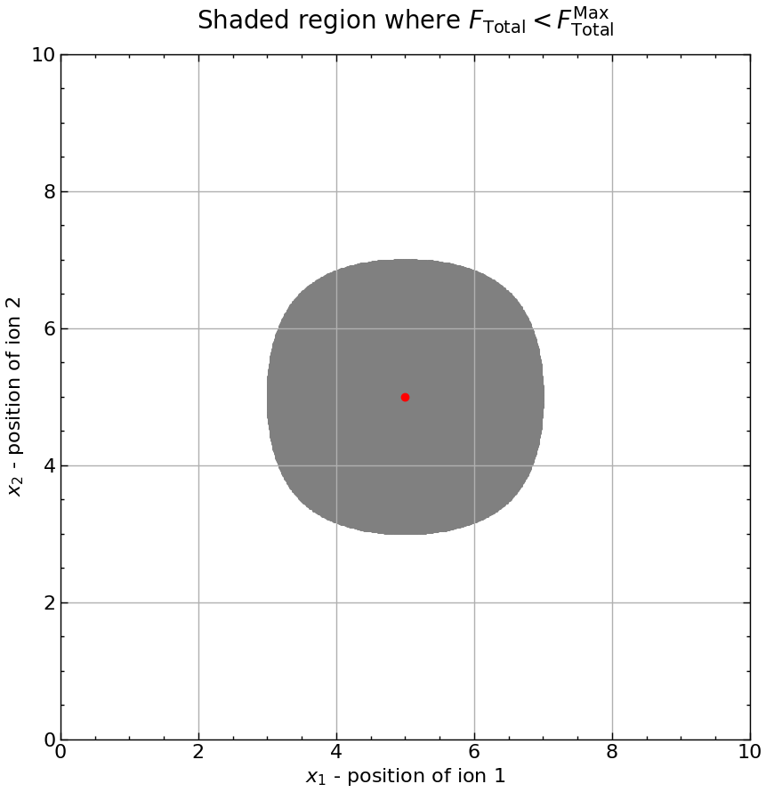
Figure 1: Region where the two-dimensional wavefunction for the two-ion system can be non-zero, in which each axis represents the position of one of the ions. Outside this region, the potential is infinite due to the QZE confinement measurements.

III Simulation Results

III.1 Ground-state solutions to the Schrödinger equation

Here, we focus on the probability densities (square of the wavefunction) corresponding to the ground-state solutions for the four different setups shown in Figs. 2 – 5. In each setup that was considered, the ions are assumed to both be protons . These probability densities serve as foundational elements for understanding the quantum behavior of ions under confinement and are crucial for subsequent QZE analyses. Each axis of the plot corresponds to the position of one of the ions, and the color represents the probability density.

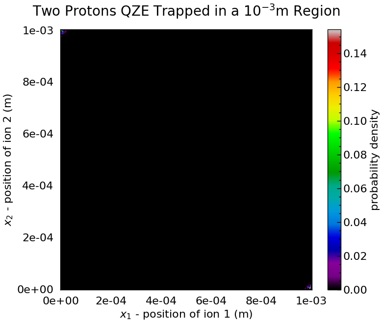
Figure 2: Ground-state probability density for $d=10^{-3}$m

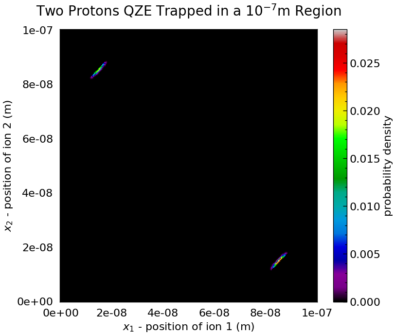
Figure 3: Ground-state probability density for $d=10^{-7}$m

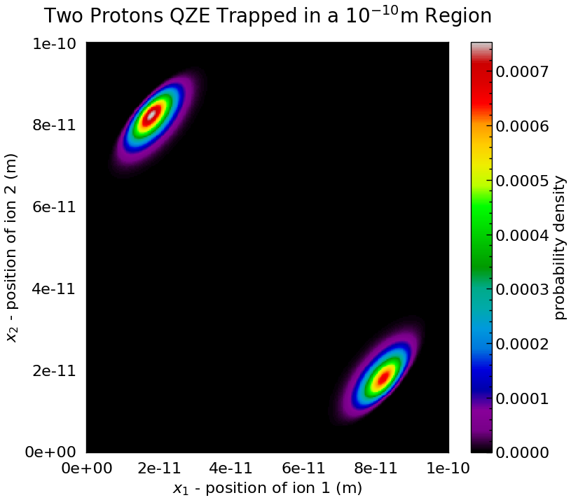
Figure 4: Ground-state probability density for $d=10^{-10}$m

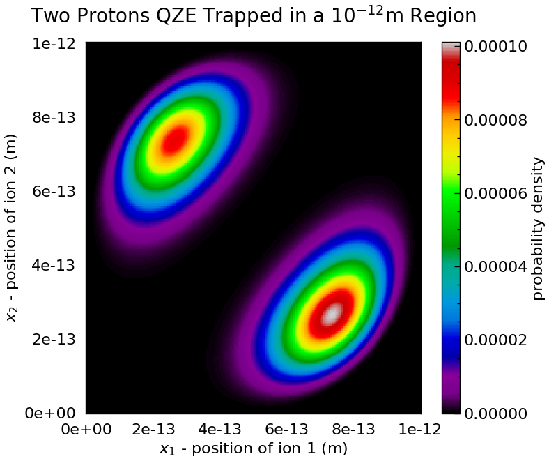
Figure 5: Ground-state probability density for $d=10^{-12}$m

Interestingly, although Setups 1 and 2 may appear less demanding from an experimental viewpoint, given their larger confinement regions, they pose computational challenges. Specifically, the larger values of $d$ in these setups require a greater number of numerical spatial grid points to obtain an accurate solution to the Schrödinger equation. This is in stark contrast to Setups 3 and 4, where the confinement regions are smaller and therefore require fewer grid points for a comparable level of accuracy.

A noteworthy observation across all setups is the localization of the ions at opposite ends of the confinement region in their respective ground states. Given the scale, a closer look at Fig. 2 may be necessary to observe this localization. This behavior aligns well with intuitive expectations, as the electrostatic repulsion between the ions will naturally drive them apart within the confinement region, thereby minimizing the system’s overall energy. The probability densities clearly depict this localization, demonstrating high probability densities at the opposite ends and significantly lower densities in the middle. This outcome is consistent with our physical intuition that the ions, which have like charges, will aim to maximize their separation within the constraints of the confinement region.

A precise understanding of energy eigenvalues is indispensable to ion trap applications, such as quantum computing. Table 1 lists the calculated ground-state energy eigenvalues for various setups within our system. For Setup 1, the energy eigenvalue is less converged due to computational limits on the number of spatial grid points.

Setup	$L$ (m)	$d$ (m)	E (J)
1	1.001e-3	1.000e-3	2.34e-25
2	1.000e-6	1.000e-7	3.30e-21
3	1.000e-6	1.000e-10	3.93e-18
4	1.000e-6	1.000e-12	8.44e-16

Table 1: Calculated ground-state energy eigenvalues for ions confined in Setups 1–4.

The proposed method offers a significant advantage for single-ion trapping. For the one-ion case, solving the Schrödinger equation and deducing the energy eigenvalues is straightforward, considering the analytical approach (as $d/L\to 1$, where we are simply solving a one-particle problem in a potential well). This simplicity and ability to precisely determine quantum states and their energies underscore the potential benefits of the proposed method, particularly for single-ion-trapping scenarios.

The central finding here is the successful theoretical demonstration of ion confinement through measurement alone, eliminating the need for external fields. This potentially addresses major challenges in ion confinement, such as the heating and control associated with fluctuating fields.

III.2 Measurement frequency to maintain the QZE barrier

An ideal QZE scenario requires continuous measurements to maintain the confinement. However, continuous measurements are not feasible. Therefore, we approximate this ideal scenario by employing frequent measurements.

To calibrate the frequency of the measurements, we introduce the concept of a leakage function, as defined in Equation (18). This quantifies the probability of ions escaping the QZE confinement region with a measurement interval $t_{\text{QZE}}$. Our strategy is to select a targeted leakage value and then adjust the frequency of the QZE confinement measurements, $f_{\text{QZE}}=1/t_{\text{QZE}}$, to achieve the targeted leakage.

Intuitively, we may expect that higher frequencies are required for smaller values of $d$. This is because the Coulomb potential is stronger and pushes the ions out of the confinement region more rapidly. This makes the task of confining ions to smaller regions more challenging in our approach. This challenge mirrors the need for larger confinement fields in traditional ion-trapping techniques. However, in our case, the requirement is more frequent measurements rather than a stronger external field, highlighting the novelty of our method.

In this study, we target a leakage of 0.1%. This value is somewhat arbitrary but serves as a reasonable benchmark. The implications of a failed QZE confinement measurement are discussed in Sec. A.1.4; however, this is not relevant to our calibrations.

The values of $f_{\text{QZE}}$ required for a number of cases are calculated. It is worth noting that calibrating $f_{\text{QZE}}$ for larger values of $d$ ($d=10^{-3}$m and $d=10^{-7}$m) presents numerical challenges, as previously explained.

Fig. 6 shows the relationship between $f_{\text{QZE}}$ and $d$, where each axis is plotted on a logarithmic scale. This helps us explore the frequency requirements for larger values of $d$, for which numerical convergence becomes an issue. We may expect that as $d\to\infty$, $f_{\text{QZE}}\to 0$, as there will be no Coulomb repulsion in this limit and we know that the energy for a particle in an infinite potential well tends to zero as the length of the well increases.

From Fig. 6, we might infer that our required frequency might be within the reach of current technology for confinement regions as small as $d=10^{-6}$m ($-6$ on the x-axis) .

Moreover, if we were examining a single-ion confinement setup, we would expect a less demanding requirement for $f_{\text{QZE}}$, allowing for smaller confinement regions, given that there would be no Coulomb repulsion. For example, for a single ion confined to $10^{-10}$m, we can relax $f_{\text{QZE}}$ by a factor of 100 and still achieve the target leakage amount.

In all cases, we expect experimental input to help determine suitable values. Clearly, the frequency requirements for the more confined setups are beyond the reach of our current technology; however, our ion confinement method might still be a preferred route for confining ions to smaller regions of space.

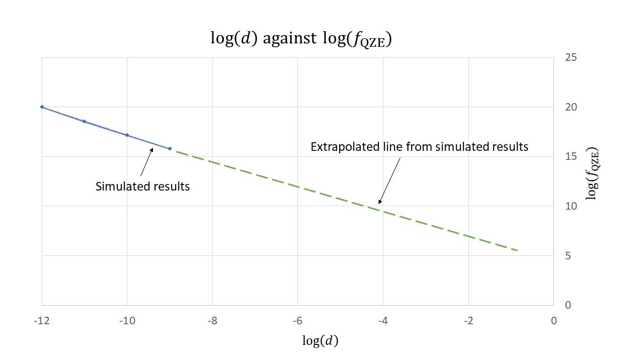
Figure 6: Relationship between $d$ and $f_{\text{QZE}}$ for simulated calculations. In each case, $f_{\text{QZE}}$ was calibrated such that $L(\psi_{d},t_{QZE})\sim 0.1\%$.

III.3 Power requirement to maintain the QZE barrier

The only energy expenditure required to maintain the QZE boundaries (ignoring state preparation and other energy losses) is the energy cost of QZE confinement measurements. Given that energy must be continuously input to keep the QZE barrier active, we can calculate the power requirement of maintaining the QZE confinement boundaries, $Q_{\text{QZE}}$, as

$$Q_{\text{QZE}}=2hf_{\text{photon}}f_{\text{QZE}}.$$ (4)

Here, we assume a pulse frequency of $f_{\text{QZE}}$ and conservatively assume that only one photon of frequency $f_{\text{photon}}$ is needed in each pulse to perform a successful QZE confinement measurement. The assumption that we only need one photon per pulse for a successful measurement of the QZE boundary is ambitious, and we would expect this number to be greater as we account for real-world factors, such as detector sensitivity, quantum efficiency, and signal-to-noise ratio. The factor of two in the above equation is derived from the fact that we have a QZE boundary at each end of $d$ .

Table 2 shows the calculated power requirements for some examples. As in the previous section, we did not include the results for large values of $d$ (i.e., Setups 1 and 2) due to numerical challenges. Furthermore, we made several assumptions about the photon frequency, $f_{\text{photon}}$, in this table. We might expect that as $d$ decreases, we may require higher-frequency photons, despite the advantages of the interferometry method employed (see Sec. A for more details). For example, in the Laser Interferometer Gravitational-Wave Observatory (LIGO) experiments [34], the photon frequency used was $10^{15}$Hz, and as such, we have assumed the same frequency for our smallest value of $d$ in the table. In any case, our assumptions about $f_{\text{photon}}$ are for illustrative purposes; however, it would be interesting to make more realistic assumptions to compare our results to those of traditional ion-trapping methods.

Note that the power requirements in Table 2 are not conservative due to the assumption about the number of photons per pulse. However, we would expect the power requirements to be much less for a single ion trap, given that there is no Coulomb repulsion from a second ion.

$d$ (m)	$f_{\text{photon}}$ (Hz)	$f_{\text{QZE}}$ (Hz)	$E_{\text{photon}}$ (J)	$Q_{\text{QZE}}$ (W)
1.00e-8	1.00e12	2.00e14	6.63e-22	2.65e-7
1.00e-9	1.00e12	6.25e15	6.63e-22	8.28e-6
1.00e-10	1.00e13	1.43e17	6.63e-21	1.89e-3
1.00e-11	1.00e14	3.33e18	6.63e-20	4.42e-1
1.00e-12	1.00e15	1.00e20	6.63e-19	1.33e2

Table 2: Illustrative lower power requirements for a variety of setups.

IV Conclusion

This study proposes a novel method for ion confinement that diverges from traditional approaches that are reliant on external forces or fields. The proposed method employs the act of measurement, derived from the principles of the QZE, to confine ions. This approach potentially addresses significant challenges in ion trapping, such as heating and quantum control by avoiding fluctuating fields.

We developed the theory behind this method and outlined an experimental setup to achieve ion confinement. Our analysis focused on two ions trapped in one dimension and covered a range of confinement distances from $10^{-12}$m to $10^{-3}$m. The obtained results suggest that achieving two-ion confinement at distances as small as $10^{-6}$m is possible with existing technology.

An advantage of our method is that it may be more suited for achieving smaller ion confinement distances, which would traditionally necessitate stronger confinement fields. Instead, our method shifts this challenge to managing increased measurement frequencies. We plan to investigate the application of our QZE-based method for achieving fusion, a long-standing problem necessitating small ion confinement distances, in a forthcoming study.

If our method is verified experimentally, it indicates new possibilities in fields such as quantum computing and cold atom physics, in which precise ion manipulation is crucial.

Future work includes extending our analysis to three-dimensional settings and multiple ions. Despite the increased computational demands, such an expansion is vital for achieving a more realistic representation of experimental scenarios. Collaborating with experimental researchers will be essential in evaluating the practical advantages of the proposed method and its potential applications.

Appendix A Methods

The methodologies employed in this study are associated with the UK patent application number GB2314602.0. The complete code and details on how to reproduce the results of this study are available on our GitHub repository: GitHub Repository.

A.1 Proposed method

We aimed to confine two ions within a cubic enclosure of edge length $L$, defined by conductor plates. Although the method is applicable to single or multiple ions, our focus was on a two-ion system to balance system complexity and calculation simplicity. The two plates acted as force sensors to determine whether both ions were inside a smaller cubic region with edge length $d<L$. This is referred to as the QZE confinement region. For clarity and simplicity, we considered a one-dimensional toy model in this study, deferring a more intricate three-dimensional model with more ions to future research.

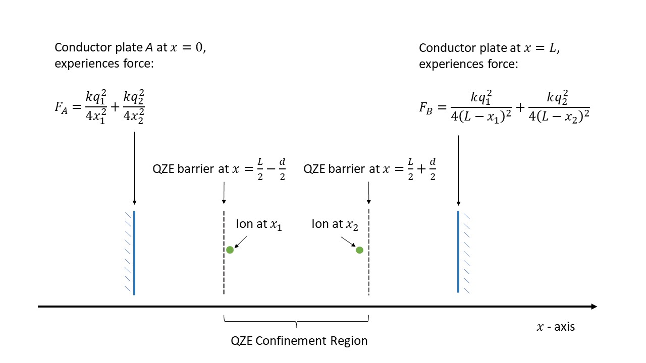
Figure 7: One-dimensional toy model. The conductor plates, set a distance $L$ apart, measure the force from the two ions. These force measurements indicate if both ions are inside the smaller QZE confinement region of length $d$.

A.1.1 One-dimensional toy model

In this one-dimensional representation, the conductor plates are regarded as infinitesimally thin boundaries on a line segment of length $L$. These plates determine whether both ions are inside a segment of length $d<L$, both centered at the same point. Fig. 7 illustrates the model. Notably, Gauss’s law ensures that the ions experience no net force from the plates, although the ions exert a force on the plates. The force exerted on a conductor plate can be determined using the method of images in electrostatics. Here, the force experienced on a conductor plate by an ion is equivalent to the attractive force exerted on the ion by a fictitious oppositely charged “mirror” ion placed symmetrically opposite on the other side of the conductor plate. Note, for the purposes of this one-dimensional representation, we do not account for the repulsive force exerted by the conductor plates on each other. This would need to be accounted for in a more realistic three-dimensional model.

A.1.2 QZE confinement measurements as a force constraint

We define the QZE confinement measurement as a measurement of the total force across the conductor plates, from which we can infer whether both ions are trapped in the QZE confinement region. The total force $F_{\text{Total}}$ on the conductor plates is given by the sum of the forces on each conductor plate:

$$F_{\text{Total}}=F_{A}+F_{B}=\frac{kq_{1}^{2}}{4x_{1}^{2}}+\frac{kq_{2}^{2}}{4x_{2}^{2}}$$

$$+\frac{kq_{1}^{2}}{4(L-x_{1})^{2}}+\frac{kq_{2}^{2}}{4(L-x_{2})^{2}}.$$ (5)

As shown in Fig. 7, the conductor plates are at positions $0$ and $L$ on the $x$-axis, with ions at $x_{1}$ and $x_{2}$ having charges of $q_{1}$ and $q_{2}$. $k$ is Coulomb’s constant in Equation (A.1.2) . The maximum value of $F_{\text{Total}}$ that can be observed such that both ions are in the QZE confinement region is obtained when the ion with the smaller charge is at the center ($L/2$) and the ion with the larger charge is at one of the QZE boundaries ($L/2-d/2$ or $L/2+d/2$). Assuming $q_{1}>q_{2}$, the force in this case is given by

$$F_{\text{Total}}^{\text{Max}}=\frac{kq_{1}^{2}}{(L-d)^{2}}+\frac{kq_{1}^{2}}{(L+d)^{2}}+\frac{2kq_{2}^{2}}{L^{2}}.$$ (6)

A successful measurement satisfying

$$F_{\text{Total}}<F_{\text{Total}}^{\text{Max}},$$ (7)

confirms that both ions are within the QZE confinement region . By performing continuous or sufficiently frequent force measurements, we ensure that the ions remain within this region. This is attributed to the QZE [29].

A.1.3 Force measurements as position measurements of conductor plates

We now discuss how the force on the conductor plates, which is critical for the QZE confinement measurements (Equation (7)), can be measured. This method requires the conductor plates (mirrors) to be treated according to quantum mechanical principles. Therefore, these plates must be engineered on a sufficiently small scale (potentially at the nanoscale) [37, 38]. In our model, we envision that each conductor plate is affixed to a spring-like mechanism. We use Hooke’s law to determine the force $F$ from the position $x$ of the conductor plate:

$$F=Kx,$$ (8)

where $K$ is the spring constant. An interferometry-based method is used to measure the position of each conductor plate. Interferometry exploits the interference of light waves to precisely measure small distances or changes in distances. The core principle behind interferometry is that light waves from a coherent source can be split into two paths and then recombined to produce interference patterns. These patterns are sensitive to the phase difference between the light waves, which is further influenced by the path length traveled by the waves [39].

Fig. 8 shows the process of measuring the position of the conductor plates . Focusing on one half of the symmetric measurement diagram, we employ a laser that emits photons of a known frequency, which then hits a beam splitter that divides it into two paths. One path reflects off a fixed mirror, serving as the reference arm, whereas the other moves toward the conductor plate itself, which also functions as a mirror. The two light beams recombine at the beam splitter and are directed to the photon detector. Any displacement of the conductor plate results in a phase difference between the two paths, producing a measurable shift in the interference pattern.

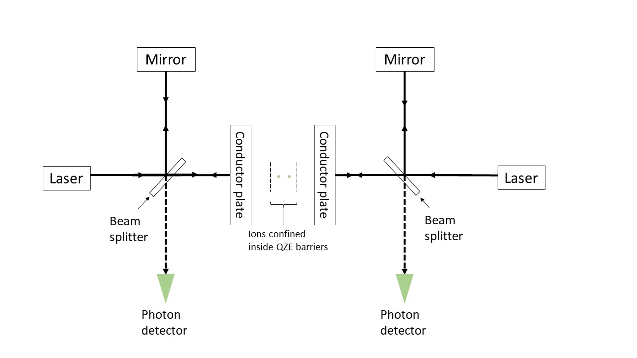
Figure 8: Interferometry setup whereby lasers can accurately measure the position of the conductor plates, which also act as mirrors to reflect the beam. This enables QZE confinement measurements on the ions.

By analyzing the interference pattern, we can precisely determine the position of the conductor plates. Through Hooke’s law (Equation (8)), we can deduce the force acting upon it and consequently gather information about the spatial configuration of the ions.

It is worth noting that while this method offers enhanced precision, it requires meticulous calibration and is sensitive to external disturbances, such as thermal fluctuations or mechanical vibrations. Furthermore, in this method, the photon wavelength need not be shorter than the desired position accuracy of the conductor plates.

A.1.4 Practical considerations

It is essential to note that the primary intent of this paper is theoretical, aiming to explore the key concepts surrounding our QZE-based method for ion confinement. The practical considerations detailed in this section offer a glimpse into the potential experimental challenges and considerations one could face when attempting to realize these concepts. While we strive to clarify the practical intricacies involved, this section does not aim to provide exhaustive solutions to the challenges presented but rather highlights them for future experimental endeavors. Considering this caveat, we discuss the practical aspects accompanying the theoretical formulations presented.

(a) Photon-induced motion. Here, we discuss the effect of the photons on the conductor plate measurements. We assume that the photon has a frequency $f_{\text{photon}}$; using the de Broglie relationship, we can ascertain its momentum:

$$p_{\text{photon}}=\frac{h}{\lambda_{\text{photon}}}=\frac{hf_{\text{photon}}}{c}.$$ (9)

Here, $p_{\text{photon}}$ is the photon momentum, $\lambda_{\text{photon}}$ is the photon wavelength, $h$ is Planck’s constant, and $c$ is the speed of light. We can calculate the force exerted by the photon on the conductor plates (mirror) as momentum transfer. Let us assume that the photon interacts with the mirror for a duration $\tau_{\text{int}}$. We can then calculate the force of the photon $F_{\text{photon}}$ on the conductor plate as

$$F_{\text{photon}}=\frac{2p_{\text{photon}}}{\tau_{\text{int}}}.$$ (10)

Here, the factor of two results from momentum conservation, given that the photon is reflected off the mirror. Estimating $\tau_{\text{int}}$ is a nuanced and intricate task, and its comprehensive treatment is beyond the scope of this study. Furthermore, the primary theoretical results presented in this paper do not rely on our ability to calculate $\tau_{\text{int}}$. Nonetheless, to facilitate our discussion and provide a tangible estimate, we offer the following heuristic approach. To gauge $\tau_{\text{int}}$, we reason that the interaction time may be related to the duration required for one full cycle of a light wave (corresponding to its wavelength) to traverse a point at the speed of light. This concept yields an approximate relation for $\tau_{\text{int}}$,

$$\tau_{\text{int}}\approx\frac{\lambda_{\text{photon}}}{c}.$$ (11)

Substituting Equations (11) and (9) into Equation (10) gives,

$$F_{\text{photon}}\approx\frac{2hf^{2}_{\text{photon}}}{c}.$$ (12)

It is important to emphasize that this is a basic approximation. In practical scenarios, particularly in quantum mechanics, the interactions between photons and mirrors may necessitate a more refined model. However, as photons exert an equivalent force on each mirror in both arms of the interferometry setup, this simplification may be considered acceptable.

(b) Force and position sensitivity requirements. It is important to understand force sensitivity requirements for the measurements and how these translate into position sensitivity requirements for the conductor plates. First, we consider accurately measuring $d$ to within $10$%. Using Equation (6), we consider the force resolution requirement as the difference between $F_{\text{Total}}^{\text{Max}}$ when $d$ is stressed by $5$% to each side,

$$F_{\text{res}}=F_{\text{Total}}^{\text{Max}}(1.05d)-F_{\text{Total}}^{\text{Max}}(0.95d).$$ (13)

Here, we explicitly state the argument of $F_{\text{Total}}^{\text{Max}}$ being varied, noting that the remaining arguments remain unchanged. As in the case of photons, we use Equation (8) to infer the movement of the conductor plate, but this time from the force exerted by the ions. Therefore, we can calculate our distance resolution requirement $x_{\text{res}}$ by simply stressing $d$ by $5$% to each side, as in Equation (13), and using Equation (8) to ascertain the impact on $x$.

(c) Measurement, pulse, and photon frequency. The frequency of QZE confinement measurements is critical in the success and precision of our setup. A distinction must be made between the rate of the QZE measurements (frequency of ion confinement measurements using the QZE) and the photon frequency used in those measurements. Specifically, a high rate of measurements does not necessarily mean that high-frequency photons are used. Our approach transmits pulses at a high frequency and maintains the duration of each pulse below the inverse of this frequency

$$t_{\text{pulse}}<\frac{1}{f_{\text{QZE}}},$$ (14)

where $t_{\text{pulse}}$ is the pulse duration and $f_{\text{QZE}}$ is the pulse frequency. The rationale behind this specification is to avoid the overlapping of pulses, thereby preventing any disruption in the interference pattern detected by our photon detector. Although higher photon frequencies provide better precision, interferometry can enable high-precision measurements without utilizing extremely high-frequency photons.

(d) Failed QZE confinement measurements. We propose two possible actions in case a QZE confinement measurement fails, meaning $F_{\text{Total}}>F_{\text{Total}}^{\text{Max}}$:

1. Introducing an external field to adjust the position of the ions or other potential quantum control techniques.

2. Using the measured $F_{\text{Total}}$ to gauge the extent to which the ions have escaped the QZE confinement region and then adjusting the QZE boundary accordingly, with the aim of bringing it back later.

(d) Response time of measurement apparatus. In our theoretical analysis, we implicitly assume an idealized scenario wherein the measuring apparatus and subsequent processing systems exhibit an instantaneous response to the dynamic state of the ions. However, in practical applications, the response time of the equipment is a non-negligible factor that can result in deviations from the predicted behavior. While our current analysis hinges on the perfection of these measurements, actual experimental setups must grapple with the finite speeds at which signals are processed and communicated. This imposes a constraint on the temporal precision achievable in the system, which could potentially influence the efficacy of the QZE in maintaining ion confinement.

(e) Initial state preparation. Here, we assume that our initial states are prepared to be in the energy ground state. This can be achieved through cooling techniques, such as laser cooling or evaporative cooling [41, 42]. By minimizing thermal fluctuations, we can effectively “force” the system into its lowest energy eigenstate, providing a well-defined starting point for our simulations.

A.1.5 Ion confinement setups

In this analysis, we consider four distinct experimental setups, as shown in Table 3. The first two setups reflect what can be accomplished using contemporary ion-trapping techniques. As we progress through the subsequent setups in the table, the experimental demands intensify. For the purposes of this analysis, we assume that the two ions being confined are both protons.

The methods used to derive $F_{\text{res}}$ and $x_{\text{res}}$ in the table are detailed in Sec. A.1.4 . For each configuration, a photon frequency of $4\times 10^{12}$Hz and an affiliated wavelength of $7.5\times 10^{-5}$m are assumed. This wavelength provides an adequate resolution for the first setup, in which the two ions are confined to $d=10^{-3}$m (given that the wavelength is close to $x_{\text{res}}=9.2\times 10^{-5}$m). However, it fails to meet the precision required for subsequent configurations. Nonetheless, this impediment can be mitigated by employing the proposed interferometric approach. Moreover, in extreme cases in which ions must be confined to atomic and subatomic distances of $10^{-10}$m and $10^{-12}$m, respectively, we require position precisions of $2.76\times 10^{-17}$m for the conductor plates. While this is highly ambitious, precisions of $10^{-19}$m have been realized at LIGO [34].

$L$ (m)	$d$ (m)	$K$ (N/m)	$F_{\text{res}}$ (N)	$x_{\text{res}}$ (m)
1.001e-3	1.000e-3	1.000e-11	9.206e-16	9.206e-5
1.000e-6	1.000e-7	1.000e-8	2.856e-18	2.856e-10
1.000e-6	1.000e-10	1.000e-7	2.761e-24	2.761e-17
1.000e-7	1.000e-12	1.000e-7	2.761e-24	2.761e-17

Table 3: Example confinement setups and associated force and position resolution requirements.

Acknowledging that our derivation of the force imparted on the mirror by the photon is an approximation (Equation (12)), we can use Hooke’s law (Equation (8)) to calculate the implied movement of the mirror using the relevant spring constant, $K$, in Table 3. Thus, we find that for Setups 1 and 2, in which we are confining ions to $10^{-3}$m and $10^{-7}$m, respectively, the distance the conductor plate moves due to the photon interaction is less than or comparable to the distance it moves due to the ions’ electric field. However, when we confine the ions to $10^{-10}$m or $10^{-12}$m (Setups 3 and 4), the photon may move the conductor plate by more than what the ions’ electromagnetic field does.

A.2 Numerical methods

A.2.1 Solving eigenstates

The problem is solved using a numerical partial differential equation (PDE). This is achieved by splitting the problem into an $N$ by $N$ grid and using a finite difference method to solve the eigenvalue/eigenvector problem. We must ensure that our grid calculations are well-behaved. It is immediately clear that $V(x_{1},x_{2})$ is not well-behaved for $x_{1}=x_{2}$. This can be rectified by regularizing $V(x_{1},x_{2})$ so that

$$V(x_{1},x_{2})=k\frac{q_{1}q_{2}}{\sqrt{(x_{1}-x_{2})^{2}+\epsilon^{2}}},$$ (15)

where $q_{1}$ and $q_{2}$ are the respective charges of each ion. $\epsilon$ is a regularization term set to $10^{-15}$m. This is justified by noting that when the denominator of Equation (15) is below this number, we expect a strong nuclear force to overcome the Coulomb repulsion [44].

Using our PDE grid, we can write

$$-\frac{\hbar^{2}}{2}\left[\frac{\psi(i+1,j)+\psi(i-1,j)-2\psi(i,j)}{m_{1}\Delta x^{2}}\right.$$

$$\left.+\frac{\psi(i,j+1)+\psi(i,j-1)-2\psi(i,j)}{m_{2}\Delta x^{2}}\right]$$

$$+k\frac{q_{1}q_{2}}{\sqrt{(i-j)^{2}\Delta x^{2}+\epsilon^{2}}}\psi(i,j)$$

$$=E\psi(i,j),$$ (16)

where $\Delta x=L/N$. The boundary conditions implied by $U(x_{1},x_{2})$ in Equation (7) can be expressed on this two-dimensional grid by setting a numerically large value for $U(x_{1},x_{2})$ at and beyond the boundary. We have one equation for each ($i,j$) pair, and the eigenvectors and associated eigenvalues can be obtained numerically [45].

A.2.2 Time evolution

To grasp the required frequency of our measurements, it is crucial to examine the time evolution of our quantum system. Continuous measurements are currently beyond our reach due to technological limitations, particularly in constructing high-frequency lasers where the challenge lies in the frequency of pulses, not the frequency of photons. Hence, the measurement frequency must be calibrated so that the wavefunction has a negligible chance of breaching the boundary between successive QZE confinement measurements.

We use the Crank–Nicolson scheme for the time-evolving system [45]:

$$\left(\hat{I}-\frac{i\Delta t}{2\hbar}\hat{H}\right)\psi(i,j,k+1)\\ =\left(\hat{I}+\frac{i\Delta t}{2\hbar}\hat{H}\right)\psi(i,j,k),$$ (17)

where $\hat{I}$ is the identity matrix, $\hat{H}$ is the Hamiltonian matrix , $\psi(i,j,k)$ is the state with $i,j$ representing the spatial grid point of each ion and $k$ representing the time step, and $\Delta t$ is the size of the time step.

A.2.3 Leakage function

The leakage function is a concept that serves as a measure of how much of the wavefunction has extended beyond a predefined boundary during the time between successive QZE confinement measurements $t_{\text{QZE}}$. This is useful for understanding the confinement of the quantum system within a certain region and calibrating a suitable value for the frequency of QZE confinement measurements, $f_{\text{QZE}}=1/t_{\text{QZE}}$.

In the continuous form, the leakage $L(\psi_{d},t_{\text{QZE}})$ is defined as

$$L(\psi_{d},t_{QZE})\\ =\int_{\text{outside}}|\psi_{d}(x_{1},x_{2},t_{QZE})|^{2}\,dx_{1}\,dx_{2}.$$ (18)

Here, $\psi_{d}(x_{1},x_{2},t_{\text{QZE}})$ represents the wavefunction in two dimensions at $t_{\text{QZE}}$ after the wavefunction was previously trapped within the region defined by $d$. The integral is calculated over and outside the region defined by $d$. Specifically, this is the region where Equation (7) is not true.

In the discrete form, the leakage $L(\psi_{d},t_{\text{QZE}})$ can be expressed as

$$L(N_{t_{\text{QZE}}})=\sum_{\text{outside}}|\psi_{d}(i,j,N_{t_{\text{QZE}}})|^{2}.$$ (19)

In this equation, $\psi(i,j,N_{t_{\text{QZE}}})$ is the value of the wavefunction at grid point $(i,j,N_{t_{\text{QZE}}})$, and $N_{t_{\text{QZE}}}$ is the time grid point associated with $t_{\text{QZE}}$. The sum is taken over grid points that lie outside the initial grid . It is clear that

$$\lim_{{t_{\text{QZE}}\to 0}}L(\psi_{d},t_{\text{QZE}})=0.$$ (20)

We hypothesize that for our purposes, having $L(\psi_{d},t_{\text{QZE}})=0$ is equivalent to having the frequency of measurements $f_{\text{QZE}}\to\infty$, noting that it is this fact that allows us to add the potential energy term $U(x_{1},x_{2})$ in Equation (2) [29].

References

- [1] Zak David Romaszko, Seokjun Hong, Martin Siegele, Reuben Kahan Puddy, Foni Raphaël Lebrun-Gallagher, Sebastian Weidt, and Winfried Karl Hensinger. Engineering of microfabricated ion traps and integration of advanced on-chip features. Nat Rev Phys, 2(6):285–299, May 2020.
- [2] Francesco Bernardini, Abhijit Chakraborty, and Carlos R Ordóñez. Quantum computing with trapped ions: a beginner’s guide. European Journal of Physics, 45(1):013001, 2023.
- [3] J. I. Cirac and P. Zoller. Quantum computations with cold trapped ions. Physical Review Letters, 74(20):4091–4094, May 1995.
- [4] I. Baumgart, J.-M. Cai, A. Retzker, M. B. Plenio, and C. Wunderlich. Ultrasensitive magnetometer using a single atom. Physical Review Letters, 116(24):240801, Jun 2016.
- [5] A. D. Ludlow, M. M. Boyd, J. Ye, E. Peik, and P. O. Schmidt. Optical atomic clocks. Reviews of Modern Physics, 87(2):637–701, Jun 2015.
- [6] D. Porras and J. I. Cirac. Effective quantum spin systems with trapped ions. Physical Review Letters, 92(20):207901, 2004.
- [7] P. H. Dawson. Quadrupole Mass Spectrometry and Its Applications. Elsevier, 1st edition, 1976.
- [8] Nicolas Schwaller, Valeria Vento, and Christophe Galland. Experimental QND measurements of complementarity on two-qubit states with IonQ and IBM Q quantum computers. Quantum Information Processing, 21(2):75, February 2022. arXiv:2105.06368 [quant-ph].
- [9] Charles London, Douglas Brown, Wenduan Xu, Sezen Vatansever, Christopher James Langmead, Dimitri Kartsaklis, Stephen Clark, and Konstantinos Meichanetzidis. Peptide Binding Classification on Quantum Computers, November 2023. arXiv:2311.15696 [quant-ph].
- [10] David Schwerdt, Lee Peleg, Yotam Shapira, Nadav Priel, Yanay Florshaim, Avram Gross, Ayelet Zalic, Gadi Afek, Nitzan Akerman, Ady Stern, Amit Ben Kish, and Roee Ozeri. Scalable architecture for trapped-ion quantum computing using rf traps and dynamic optical potentials. 2024. arXiv:2311.01168 [physics, physics:quant-ph].
- [11] Jan Benhelm, Gerhard Kirchmair, Christian F. Roos, and Rainer Blatt. Towards fault-tolerant quantum computing with trapped ions. Nature Physics, 4(6):463–466, June 2008.
- [12] Evan P. G. Gale, Zain Mehdi, Lachlan M. Oberg, Alexander K. Ratcliffe, Simon A. Haine, and Joseph J. Hope. Optimized fast gates for quantum computing with trapped ions. Physical Review A, 101(5), May 2020.
- [13] Yang Wang, Selwyn Simsek, Thomas M. Gatterman, Justin A. Gerber, Kevin Gilmore, Dan Gresh, Nathan Hewitt, Chandler V. Horst, Mitchell Matheny, Tanner Mengle, Brian Neyenhuis, and Ben Criger. Fault-tolerant one-bit addition with the smallest interesting colour code. 2023. arXiv:2309.09893 [quant-ph].
- [14] J. Werschnik and E. K. U. Gross. Quantum optimal control theory. 2007. arXiv:0707.1883 [quant-ph].
- [15] Christiane P. Koch, Ugo Boscain, Tommaso Calarco, Gunther Dirr, Stefan Filipp, Steffen J. Glaser, Ronnie Kosloff, Simone Montangero, Thomas Schulte-Herbrüggen, Dominique Sugny, and Frank K. Wilhelm. Quantum optimal control in quantum technologies. strategic report on current status, visions and goals for research in europe. EPJ Quantum Technology, 9(1), July 2022.
- [16] Jing-Bo Wang. Robust quantum control for higher order coupling term in trapped ions. 2022. arXiv:2211.08150 [quant-ph].
- [17] Denys I Bondar, Kurt Jacobs, Georgios Korpas, Jakub Marecek, et al. Quantum optimal control via polynomial optimization: A globally convergent approach. 2022. arXiv:2209.05790 [quant-ph].
- [18] Michael H Goerz, Sebastián C Carrasco, and Vladimir S Malinovsky. Quantum optimal control via semi-automatic differentiation. Quantum, 6:871, 2022.
- [19] Wolfgang Paul. Electromagnetic traps for charged and neutral particles. Reviews of Modern Physics, 62(3):531, 1990.
- [20] D.J. Wineland, C. Monroe, W.M. Itano, D. Leibfried, B.E. King, and D.M. Meekhof. Experimental issues in coherent quantum-state manipulation of trapped atomic ions. Journal of Research of the National Institute of Standards and Technology, 103(3):259, May 1998.
- [21] Colin D. Bruzewicz, John Chiaverini, Robert McConnell, and Jeremy M. Sage. Trapped-Ion Quantum Computing: Progress and Challenges. Applied Physics Reviews, 6(2):021314, June 2019. arXiv:1904.04178 [physics, physics:quant-ph].
- [22] D. Trypogeorgos, A. Valdés-Curiel, N. Lundblad, and I. B. Spielman. Synthetic clock transitions via continuous dynamical decoupling. Phys. Rev. A, 97(1):013407, January 2018.
- [23] Xinfang Zhang, Baoquan Ou, Ting Chen, Yi Xie, Wei Wu, and Pingxing Chen. Versatile surface ion trap for effective cooling and large-scale trapping of ions. 2019. arXiv:1901.11250 [physics].
- [24] Itano, W. M., Heinzen, D. J., Bollinger, J. J., and Wineland, D. J. Quantum zeno effect. Physical Review A, 41(5):2295–2300, 1990.
- [25] Facchi, P. and Pascazio, S. Quantum zeno subspaces. Physical Review Letters, 89:080401, 2002.
- [26] D. J. Bedingham and J. J. Halliwell. Classical Limit of the Quantum Zeno Effect by Environmental Decoherence. Physical Review A, 89(4):042116, April 2014. arXiv:1402.4365 [quant-ph].
- [27] It is recognized that the dynamic Casimir effect could theoretically induce electromagnetic effects even in the absence of external fields. However, this effect is expected to be very small for our setup.
- [28] D. J. Griffiths. Introduction to quantum mechanics. Cambridge University Press, page 1, 1985.
- [29] Facchi, P. and Pascazio, S. Quantum zeno dynamics: Mathematical and physical aspects. Journal of Physics A: Mathematical and Theoretical, 41(49):493001, 2008.
- [30] In fact, when the ratio , the shape tends to become a square. This is expected because in this limit, the ions are simply bound by the conductor plates at the boundaries of a one-dimensional line, implying that the wavefunction is bound by a two-dimensional square.
- [31] We assume opposite spins for each proton to avoid additional constraints on the symmetry of our two-proton wavefunction due to the Pauli exclusion principle.
- [32] This is inferred by linear extrapolation of the simulation results. Numerical simulations suggest that confinement can be achieved at lower frequencies; however, the convergence of the results is less robust due to numerical limitations.
- [33] This factor of two will increase in a more realistic three-dimensional setup.
- [34] B. P. et al. Abbott. Observation of gravitational waves from a binary black hole merger. Physical Review Letters, 116(6):061102, February 2016.
- [35] is a legitimate observable, as it is a real-valued function of position within our domain of interest, satisfying the criteria for a Hermitian operator.
- [36] This formula would need an adjustment in a more realistic model that accounts for the repulsive force exerted by the conductor plates on each other due to their respective induced charges.
- [37] Max Planck Institute of Quantum Optics. A mirror made of atoms. https://www.mpq.mpg.de/6290015/07-a-mirror-made-of-atoms, 2020.
- [38] Jun Rui, David Wei, Antonio Rubio-Abadal, Simon Hollerith, Johannes Zeiher, Dan M. Stamper-Kurn, Christian Gross, and Immanuel Bloch. A subradiant optical mirror formed by a single structured atomic layer. Nature, 583(7816):369–374, July 2020.
- [39] Rajpal S Sirohi. Introduction to Optical Metrology. CRC Press, 2015.
- [40] Fig 8 shows two photon detectors, whereas if we were measuring the total force according to Equation (A.1.2), we would need only one detector to measure the interference pattern of a recombined beam. However, an alternative formulation of the force constraint on each conductor plate, necessitating two photon detectors, is possible.
- [41] Sideband Cooling Micromechanical Motion to the Quantum Ground State. Nature, 475(7356):359–363, July 2011. arXiv:1103.2144 [quant-ph].
- [42] E. S. Shuman, J. F. Barry, and D. DeMille. Laser cooling of a diatomic molecule. Nature, 467(7317):820–823, October 2010. arXiv:1103.6004 [physics].
- [43] While we stress by % to each side in the table to calculate , for Setup 1, our stress values for are m and m. This is still a % stress, but it ensures that we do not use a value for that is greater than .
- [44] Samuel S. M. Wong. Introductory Nuclear Physics. Wiley, 1998.
- [45] William H. Press, Saul A. Teukolsky, William T. Vetterling, and Brian P. Flannery. Numerical Recipes: The Art of Scientific Computing. Cambridge University Press, 3rd edition, 2007.
- [46] Here, the Hamiltonian does not include the effective potential term , as we are evolving the state between successive QZE confinement measurements.
- [47] As for the continuous case, the integral is over the region outside that defined by (where Equation (7) is not true).