Deconfinement transitions in three-dimensional compact lattice Abelian Higgs models with multiple-charge scalar fields

Abstract

We investigate the nature of the deconfinement transitions in three-dimensional lattice Abelian Higgs models, in which a complex scalar field of integer charge $Q\geq 2$ is minimally coupled with a compact $U(1)$ gauge field. Their phase diagram presents two phases separated by a transition line where static charges $q$, with $q<Q$, deconfine. We argue that these deconfinement transitions belong to the same universality class as transitions in generic three-dimensional ${\mathbb{Z}}_{Q}$ gauge models. In particular, they are Ising-like for $Q=2$, of first order for $Q=3$, and belong to the three-dimensional gauge $XY$ universality class for $Q\geq 4$. This general scenario is supported by numerical finite-size scaling analyses of the energy cumulants for $Q=2$, $Q=4$, and $Q=6$.

I Introduction

Three-dimensional (3D) Abelian Higgs (AH) gauge models, in which charged scalar fields are coupled with an Abelian gauge field, provide effective models for several emergent collective phenomena in condensed-matter physics Anderson-book ; Wen-book ; Sachdev-19 . The phase structure of this class of models has been extensively studied, see, e.g., Refs. HLM-74 ; FS-79 ; DH-81 ; FMS-81 ; DHMNP-81 ; BF-81 ; CC-82 ; BF-83 ; FM-83 ; KK-85 ; KK-86 ; BN-86 ; BN-86-b ; BN-87 ; RS-90 ; MS-90 ; KKS-94 ; BFLLW-96 ; HT-96 ; FH-96 ; IKK-96 ; KKLP-98 ; OT-98 ; CN-99 ; HS-00 ; SSS-02 ; SM-02 ; KNS-02 ; MHS-02 ; SSSNH-02 ; SSNHS-03 ; MZ-03 ; NRR-03 ; MV-04 ; SBSVF-04 ; NSSS-04 ; SSS-04 ; HW-05 ; WBJSS-05 ; CFIS-05 ; TIM-05 ; TIM-06 ; CIS-06 ; KPST-06 ; Herbut-book ; Sandvik-07 ; WBJS-08 ; MK-08 ; JNCW-08 ; MV-08 ; KMPST-08 ; CAP-08 ; KS-08 ; ODHIM-09 ; LSK-09 ; CGTAB-09 ; CA-10 ; BDA-10 ; Sandvik-10 ; GS-10 ; IMH-12 ; Kaul-12 ; KS-12 ; BMK-13 ; HBBS-13 ; Bartosch-13 ; HSOMLWTK-13 ; CHDKPS-13 ; PDA-13 ; BS-13 ; NCSOS-15 ; NSCOS-15 ; SP-15 ; SGS-16 ; WNMXS-17 ; FH-17 ; PV-19-CP ; IZMHS-19 ; PV-19-AH3d ; SN-19 ; Sachdev-19 ; PV-20-largeNCP ; SZ-20 ; PV-20-mfcp ; BPV-20-hcAH ; BPV-21 ; BPV-21-bgs ; BPV-21-ncAH ; WB-21 ; BPV-22-mpf ; BPV-22 ; BPV-22-dis ; BPV-23b ; SZJSM-23 ; BPV-23d ; BPV-24 . It has been realized that a crucial role is played by topological properties. Indeed, the phase diagram and the nature of the transitions depend on the compact or noncompact nature of the gauge fields FS-79 ; DH-81 ; KK-85 ; BN-87 ; NRR-03 ; BPV-22 , and, in compact lattice models, on the charge of the scalar fields FS-79 ; BF-81 ; SSNHS-03 ; BPV-20-hcAH and on the presence or absence of topological defects such as monopoles MS-90 ; MV-04 ; PV-19-CP ; PV-20-mfcp .

We consider compact lattice AH (CLAH) models defined on 3D cubic lattices. The partition function reads

$$Z=\sum_{\{z,\lambda\}}e^{-\beta H},\qquad H=JH_{z}+KH_{\lambda},$$ (1)

$$H_{z}=-2\sum_{{\bm{x}},\mu}{\rm Re}\,\bar{z}_{\bm{x}}\lambda_{{\bm{x}},\mu}^{Q}z_{{\bm{x}}+\hat{\mu}},$$ (2)

$$H_{\lambda}=-2\sum_{{\bm{x}},\mu>\nu}{\rm Re}\,\Pi_{{\bm{x}},\mu\nu},$$ (3)

$$\Pi_{{\bm{x}},\mu\nu}=\lambda_{{\bm{x}},{\mu}}\,\lambda_{{\bm{x}}+\hat{\mu},{\nu}}\,\bar{\lambda}_{{\bm{x}}+\hat{\nu},{\mu}}\,\bar{\lambda}_{{\bm{x}},{\nu}},$$ (4)

where $\lambda_{{\bm{x}},\mu}\in U(1)$ are phases (unit-length complex variables) associated with each lattice link (starting at site ${\bm{x}}$ along one of the lattice direction, $\mu=1,2,3$), $z_{\bm{x}}$ are unit-length complex variables associated with each lattice site, and $Q\in\mathbb{N}$ is the charge of the complex scalar field $z_{\bm{x}}$. Without loss of generality, the inverse temperature $\beta=1/(k_{B}T)$ can be absorbed in the definition of the couplings $J$ and $K$, formally setting $\beta=1$ in the partition function (1). The model is invariant under U(1) gauge transformations, $z_{\bm{x}}\to U_{\bm{x}}z_{\bm{x}}$, $\lambda_{{\bm{x}},\mu}=U_{\bm{x}}\lambda_{{\bm{x}},\mu}\bar{U}_{{\bm{x}}+\hat{\mu}}$, where $U_{\bm{x}}$ is a phase. The CLAH model can also be rewritten in terms of the gauge fields only, by exploiting the gauge invariance. Indeed, by appropriate gauge transformations, we can set $z_{\bm{x}}=1$ everywhere (the so-called unitary gauge), obtaining the unitary-gauge CLAH Hamiltonian

$$H_{\rm ug}=-2J\sum_{{\bm{x}}\mu}\hbox{Re}\ \lambda_{{\bm{x}},\mu}^{Q}+KH_{\lambda},$$ (5)

which presents a residual invariance under local ${\mathbb{Z}}_{Q}$ gauge transformations, i.e., under transformations $\lambda_{{\bm{x}},\mu}=V_{\bm{x}}\lambda_{{\bm{x}},\mu}\bar{V}_{{\bm{x}}+\hat{\mu}}$ with $V_{\bm{x}}\in{\mathbb{Z}}_{Q}$, i.e., such that $V_{\bm{x}}^{Q}=1$.

Figure 1: Sketch of the $J$-$K$ phase diagram of the 3D one-component CLAH model, in which a compact $U(1)$ gauge field is coupled with a (unit-length) complex scalar field with charge $Q\geq 2$. A confined phase (for small $J$ or small $K$) and a deconfined phase (for large $J$ and $K$) are present, separated by a deconfinement transition line. For $K\to\infty$ and $J\to\infty$ the model reduces to the $XY$ vector model and to the lattice ${\mathbb{Z}}_{Q}$ gauge model with Wilson action, respectively. See Sec. II for more details.

The phase diagrams of the CLAH models with $Q=1$ and $Q>1$ differ significantly FS-79 ; SSNHS-03 . While the $Q=1$ model has only one thermodynamic phase, for $Q\geq 2$ two different phases occur. They are divided by a transition line where the charged degrees of freedom with $q<Q$ deconfine. A sketch of the phase diagram for $Q\geq 2$ is shown in Fig. 1. The deconfinement transition line is expected to connect the transition points of the models obtained for $J\to\infty$ and $K\to\infty$, respectively, i.e., the ${\mathbb{Z}}_{Q}$ gauge model and the standard $XY$ model FS-79 ; SSNHS-03 .

In the present paper we investigate the nature of the deconfinement transition line, and, in particular, its universal critical properties when the transitions are continuous. Numerical results for the one-component CLAH model have been reported in Refs. BF-81 ; SSSNH-02 ; SSNHS-03 for several values of $Q\geq 2$. On the basis of analyses of Monte Carlo (MC) data, Ref. SSNHS-03 claimed that the critical behavior along the deconfinement transition line is not universal, but it is controlled by a line of fixed points. So, critical exponents change continuously along the transition line, varying from those of the ${\mathbb{Z}}_{Q}$ gauge transition at $J=\infty$ to those of the $XY$ transition at $K=\infty$.

This type of behavior, if confirmed, would be quite unusual for 3D transitions. Indeed, while there are several examples of fixed-point lines in two dimensions—exact results have been obtained for the eight-vertex model Baxter-book , the Ashkin-Teller model AT-43 ; KW-71 ; MM-23 , and the low-temperature spin-wave phase of the $XY$ model  KT-73 ; Berezinskii-70 ; Kosterlitz-74 ; JKKN-77 —there is no robust evidence (i.e., exact results or compelling physical arguments) that some transition lines in 3D models are associated with lines of fixed points. Therefore, it is important to review and improve the previous numerical results, given that the existence of a line of fixed points would represent a new phenomenon in three dimensions.

In this paper we return to this issue, performing a detailed finite-size scaling (FSS) analysis of MC data for $Q=2$, $Q=4$, and $Q=6$. We anticipate that the results of our analyses are consistent with the more conventional 3D scenario: The universality class of the deconfinement transitions does not change along the line. Their critical behavior is the same as in generic lattice ${\mathbb{Z}}_{Q}$ gauge models, so the transitions belong to the Ising and $XY$ universality classes for $Q=2$ and $Q\geq 4$, respectively. This is the same critical behavior observed in ${\mathbb{Z}}_{Q}$ gauge models obtained in the $J\to\infty$ limit with a notable exception, the case $Q=4$. This is related to the fact that the ${\mathbb{Z}}_{4}$ gauge model obtained for $J\to\infty$ is not a generic ${\mathbb{Z}}_{4}$ gauge model, but a particular one that is equivalent to two decoupled Ising gauge models. Instead, along the deconfinement line, the critical behavior of the $Q=4$ model is expected to be that of a generic ${\mathbb{Z}}_{4}$ gauge model, which undergoes an $XY$ transition, as for $Q>4$.

We stress that, since numerical analyses based on MC simulations only consider a limited range of lattice sizes or correlation lengths (the same is true for experiments), the control of the nonuniversal scaling corrections to the asymptotic critical behavior is crucial to check universality. Without a proper handling of these corrections, inaccurate estimates of critical universal parameters are obtained, leading to apparent violations of universality. In particular, we point out the existence of significant crossover effects for large values of $K$, arising from the unstable $XY$ vector critical behavior present for $K=\infty$. They may hide the universal behavior when analyzing numerical data for relatively small lattice sizes.

The paper is organized as follows. In Sec. II we discuss the phase diagram of CLAH models with $Q\geq 2$, and put forward a general scenario for the deconfinement transitions. In Sec. III we outline the main features of our FSS analyses of the energy cumulants. In Sec. IV we report our FSS analyses of the MC data for $Q=2$, $Q=4$, and $Q=6$. In Sec. V we summarize and draw our conclusions. We also compare the results for the one-component CLAH models with those for other lattice AH models. We also add a number of appendices, reporting useful results that characterize the universality class of ${\mathbb{Z}}_{Q}$ gauge models and of gauge $XY$ models.

II Phase diagrams of multicharge CLAH models

In this section we discuss the phase diagram of the CLAH model defined in Eq. (1) for $Q\geq 2$, as a function of the Hamiltonian parameters $J$ and $K$ (as mentioned we set $\beta=1$), see Fig. 1. We assume $K\geq 0$, so the parameter $K$ plays the role of inverse square gauge coupling, i.e., $K\sim g^{-2}$. Moreover, since the phase diagram is symmetric for $J\to-J$, as can be seen by using the field redefinition $z_{\bm{x}}\to(-1)^{x_{1}+x_{2}+x_{3}}z_{\bm{x}}$, we assume $J\geq 0$.

For $Q\geq 2$, two different phases are present, which are distinguished by the confinement properties of the charged excitations with $q<Q$. Indeed, the transition line separating these two phases is related to the deconfinement of the charged degrees of freedom with $q<Q$ and, in particular, to the behavior of the unit-charge Wilson loops $W_{\cal C}=\prod_{\ell\in\cal C}\lambda_{\ell}$, where $\cal C$ is a closed lattice loop. For $Q\geq 2$, the Wilson loop for unit-charge sources obeys the area law in the confined phase and the perimeter law in the deconfined phase. For $Q=1$ the area law never holds, due to the screening of the charged scalar modes, so only the deconfined phase is present. Note that the nontrivial dependence on the charge $Q$ is strictly related to the compact gauge action in which $\lambda_{{\bm{x}},\mu}\in U(1)$ is used. In noncompact formulations, the gauge field is a real field $A_{{\bm{x}},\mu}$, and the charge $Q$ can be eliminated by a redefinition of $A_{{\bm{x}},\mu}$ and $K$.

For $J\to\infty$ the model with $Q\geq 2$ is equivalent to the lattice ${\mathbb{Z}}_{Q}$ gauge model with Wilson action Wegner-71 ; SSNHS-03 ; BPV-20-hcAH . Indeed, if we start from the unitary-gauge Hamiltonian (5), only fields satisfying $\lambda_{{\bm{x}},\mu}^{Q}=1$ are allowed for $J\to\infty$. Therefore, we obtain a gauge theory with link variables

$$\rho_{{\bm{x}},\mu}=\exp(2\pi in_{{\bm{x}},\mu}/Q),\qquad n_{{\bm{x}},\mu}=1,...,Q,$$ (6)

and Hamiltonian

$$H_{{\mathbb{Z}}_{Q}}=-2K\sum_{{\bm{x}},\mu>\nu}{\rm Re}\,(\rho_{{\bm{x}},{\mu}}\,\rho_{{\bm{x}}+\hat{\mu},{\nu}}\,\bar{\rho}_{{\bm{x}}+\hat{\nu},{\mu}}\,\bar{\rho}_{{\bm{x}},{\nu}}).$$ (7)

The $\mathbb{Z}_{Q}$ gauge model (7) has a topological transition for a finite $K=K_{{\mathbb{Z}}_{Q}}$ Bhanot:1980pc ; Borisenko:2013xna .

The $\mathbb{Z}_{Q}$ gauge model is dual to a specific $Q$-state clock model Savit-80 , with $\mathbb{Z}_{Q}$ spin variables $\exp(2\pi in_{\bm{x}}/Q)$ (where $n_{\bm{x}}=1,...,Q$) associated with the sites, and a Hamiltonian which is symmetric under global ${\mathbb{Z}}_{Q}$ transformations. The 2-state clock model is equivalent to the Ising model, while the 3-state clock model is equivalent to the 3-state Potts model, which undergoes a first-order transition. The nature of the transitions for $Q\geq 4$ can be understood using the Landau-Ginzburg-Wilson (LGW) approach. The LGW Hamiltonian for a $\mathbb{Z}_{Q}$-symmetric spin system can be written as BPV-22-dis

$${\cal H}_{\mathbb{Z}_{Q}}=|\partial_{\mu}\Phi|^{2}+r\,|\Phi|^{2}+u\,|\Phi|^{4}+v\,(\Phi^{Q}+\bar{\Phi}^{Q}),$$ (8)

where $\Phi({\bm{x}})$ is a complex field. Note that ${\cal H}_{\mathbb{Z}_{Q}}$ is also invariant under the transformation $\Phi\to\bar{\Phi}$, which, however, does not play any role at criticality. The $Q$-dependent potential has dimension $Q$ and is therefore irrelevant for $Q>4$. We can thus set $v=0$, obtaining the standard $\Phi^{4}$ theory for a complex field. We thus predict an $XY$ critical behavior and an effective enlargement of the symmetry at the transition.

For $Q=4$, the $Q$-dependent potential has dimension four and represents a cubic anisotropy. The renormalization-group (RG) flow of model (8) with $Q=4$ has been studied by using different approaches, see, e.g., Refs. Aharony-76 ; PV-02 ; CPV-00 ; Hasenbusch-23 . It turns out that the stable fixed point is again the $XY$ fixed point with $v=0$. The anisotropic interaction with coefficient $v$ gives only rise to scaling corrections. However, due to the small absolute value of the corresponding RG dimension CPV-00 ; CPV-03 ; HV-11 $y_{v}=-0.108(6)$, these scaling corrections are expected to decay slowly. Beside the stable fixed point along the line $v=0$, the LGW model admits also an unstable nontrivial fixed point along the line $w=u-6v=0$, where the LGW Hamiltonian can be written as the sum of two identical LGW Hamiltonians with a real scalar field, so that this fixed point corresponds to an Ising critical behavior. The parameter $w$ parametrizes a relevant perturbation of the Ising fixed point with RG dimension $y_{w}=d-2/\nu_{I}=0.17475(2)$, where KPSV-16 $\nu_{I}=0.629971(4)$ is the Ising critical exponent. The LGW analysis therefore predicts that generic $\mathbb{Z}_{4}$ invariant clock models undergo $XY$ transitions. However, the standard $\mathbb{Z}_{4}$ clock model can be exactly rewritten as a sum of two Ising models HS-03 , and thus it exactly corresponds to the LGW theory with $w=0$, hence it undergoes an Ising transition.

We can use duality and the above results for $Q$-state clock models to predict the nature of the transitions in ${\mathbb{Z}}_{Q}$ gauge models, corresponding to the $J\to\infty$ limit of the CLAH models. For $Q=2$ we have an Ising transition for $J=\infty$ and $K_{{\mathbb{Z}}_{2}}=0.380706646(6)$ Wegner-71 ; BPV-20-hcAH ; FXL-18 , while for $Q=3$, the transition should be of first order. The ${\mathbb{Z}}_{4}$ gauge model is dual to the standard ${\mathbb{Z}}_{4}$ clock model, hence it should undergo an Ising transition. This result also follows from the exact relation

$$Z_{{\mathbb{Z}}_{4}}(K)=Z_{{\mathbb{Z}}_{2}}(K/2)^{2},\quad Z_{{\mathbb{Z}}_{Q}}(K)=\sum_{\{\rho\}}e^{-H_{{\mathbb{Z}}_{Q}}(K)},$$ (9)

between the partition functions of the ${\mathbb{Z}}_{4}$ and ${\mathbb{Z}}_{2}$ gauge models defined by the Hamiltonian (7), which is demonstrated in App. A. This relation also implies that the transition point of the ${\mathbb{Z}}_{4}$ gauge model is located at $K_{{\mathbb{Z}}_{4}}=2K_{{\mathbb{Z}}_{2}}=0.761413292(12)$. For $Q>4$ the transitions of the lattice ${\mathbb{Z}}_{Q}$ gauge models belong to the 3D $XY$ universality class HS-03 ; BPV-20-hcAH . For $Q=6$ the transition occurs at $K_{{\mathbb{Z}}_{6}}=1.50342(4)$ Borisenko:2013xna . Moreover, for large $Q$ we have BPV-22

$$K_{{\mathbb{Z}}_{Q}}\approx\frac{K_{IXY}}{2}Q^{2},\qquad K_{IXY}=0.076051(2),$$ (10)

where $K_{IXY}$ is the critical point of the inverted $XY$ model that represents the $J\to\infty$ limit of the noncompact lattice AH model.

The previous discussion allows us to conclude that the limiting ${\mathbb{Z}}_{Q}$ gauge model with Hamiltonian (7) undergoes an Ising transition for $Q=2$ and 4, and an $XY$ transition for $Q\geq 5$. It is however important to stress that this identification is done using the duality between the gauge and the spin system, and that duality only maps the free energy and the related thermal observables. Strictly speaking, the Ising and $XY$ fixed points that control the critical behavior of ${\mathbb{Z}}_{Q}$ gauge models differ from the Ising and $XY$ fixed points that are relevant for the corresponding ${\mathbb{Z}}_{Q}$ clock models. Indeed, they represent fixed points obtained by performing RG transformations on two different classes of Hamiltonians—those with local and global ${\mathbb{Z}}_{Q}$ symmetry, respectively. We have used the same name because of the existence of the duality transformation, which, however, only relates the thermal sectors of the two models. There are both relevant and irrelevant operators that are unrelated: for instance, the magnetic sector in the spin universality class has no counterpart in the gauge universality class. In the following, to avoid confusion, we distinguish the gauge $XY$ from the spin $XY$ universality class by writing $XY_{G}$ in the gauge case. No suffix will be used for the Ising case, as no confusion can arise: in this work we always refer to the Ising-gauge universality class.

For $K\to\infty$, the plaquette term becomes trivial, i.e., $\Pi_{{\bm{x}},\mu\nu}=1$ everywhere. Therefore, in the thermodynamic limit, we can set $\lambda_{{\bm{x}},\mu}=1$ modulo gauge transformations (in a finite volume there are some subtleties that are discussed in App. B). The scalar Hamiltonian becomes

$$H_{XY}(J)=-2J\sum_{{\bm{x}},\mu}{\rm Re}\,\bar{z}_{\bm{x}}z_{{\bm{x}}+\hat{\mu}},$$ (11)

for any $Q$. The model undergoes therefore an $XY$ vector transition at Hasenbusch-19 ; CHPV-06 ; DBN-05 $J_{XY}=0.22708234(9)$, for any $Q$.

The $XY$ spin fixed point that controls the critical behavior in the model (11) is unstable with respect to the addition of Abelian gauge variables BPV-22 . This can be shown by computing the RG dimension of the gauge operator that drives the system out of the fixed point in the AH field theory BPV-21-ncAH . To all orders of perturbation theory in the $\varepsilon=4-d$ expansion, we obtain BPV-21-ncAH $y_{\alpha}=4-d$ ($y_{\alpha}=1$ in three dimensions) for the crossover exponent associated with the squared gauge coupling $\alpha\equiv g^{2}\sim 1/K$. The RG dimension $y_{\alpha}$ corresponds to the energy dimension of the gauge coupling $\alpha$. Therefore, in the large-$K$ limit, the gauge field gives rise to an intrinsic crossover scale $\xi_{\alpha}\sim K$. If the correlation length $\xi$ or the size of the system $L$ satisfies $\xi\lesssim\xi_{\alpha}$ or $L\lesssim\xi_{\alpha}$, significant crossover effects with an apparent $XY$ behavior can be observed.

We now turn to discuss the deconfinement transitions for finite $J$ and $K$. A natural working hypothesis is that all transitions along the line running from $[J=\infty,K_{{\mathbb{Z}}_{Q}}]$ to $[J_{XY},K=\infty]$ have the same universal features—as we have already mentioned, a line of fixed points seems unlikely in 3D. Given that the CLAH model is equivalent to a purely gauge model with ${\mathbb{Z}}_{Q}$ gauge symmetry in the unitary gauge, see Eq. (5), the most natural hypothesis is that the finite-$J$ deconfinement transitions have the same universal features as the topological transition in the ${\mathbb{Z}}_{Q}$ gauge model obtained for $J\to\infty$. In this scenario we would expect Ising deconfinement transitions for $Q=2$, first-order transitions for $Q=3$, since the $J\to\infty$ transition is of first order, and $XY_{G}$ transitions for any $Q>4$.

We do not expect the above scenario to work for $Q=4$. Indeed, as we have discussed above, the $\mathbb{Z}_{4}$ gauge model (7) is not a generic $\mathbb{Z}_{4}$ gauge model: because of the identity (9), its partition function is equivalent to that of two decoupled Ising gauge models. The addition of the scalar field spoils this factorization [this is more easily seen using the unitary-gauge Hamiltonian (5)]: Barring unexpected cancellations, the finite-$J$ scalar Hamiltonian should represent a relevant perturbation of the $J\to\infty$ Ising fixed point. Therefore, the finite-$J$ transitions should be controlled by the stable $XY_{G}$ fixed point also for $Q=4$. However, for large $J$ we expect significant crossover effects due to the nearby Ising gauge transition, given the small RG dimension, $y_{w}\approx 0.17$, of the relevant perturbation of the unstable Ising fixed point.

It is important to observe that the critical behavior for $Q\geq 4$ is quite peculiar, as the addition of Abelian gauge fields to the spin (clock) model drives the system out of the unstable spin $XY$ fixed point towards the related stable $XY_{G}$ fixed point. To understand this behavior, it is important to remember that the spin $XY$ and the $XY_{G}$ fixed points differ, as duality only relates their thermal sectors. In particular, the relevant gauge perturbation of the spin $XY$ fixed point does not have a counterpart at the $XY_{G}$ fixed point, given that the latter is stable—this is our working hypothesis that is confirmed by the numerical results—when scalar degrees of freedom are added.

Figure 2: Sketch of the $J$-$K$ phase diagram of the 3D multicomponent CLAH model, in which a compact U(1) gauge field is coupled with an $N$-component unit-length complex scalar field of charge $Q\geq 2$, for generic $N\geq 2$. There are three phases, the disordered-confined (DC), the ordered-deconfined (OD), and the ordered-confined (OC) phases. The AH model is equivalent to the $CP^{N-1}$ model for $K=0$, to the $O(2N)$ vector model for $K\to\infty$. For $J\to\infty$ and $Q\geq 2$, we obtain the lattice ${\mathbb{Z}}_{Q}$ gauge model as in the one-component case.

As we shall see, the numerical FSS analyses for $Q=2,\,4,\,6$ that we report in the next section are substantially consistent with the above scenario. No anomalous violations of universality along the deconfinement line are observed. Indeed, all deviations can be explained as standard scaling corrections to the asymptotic critical behavior. It is worth mentioning that the noncompact lattice AH model, which can be seen as the $Q\to\infty$ limit of the CLAH model  BPV-22 , has an analogous phase diagram, with an $XY_{G}$ deconfinement transition line.

We finally mention that a similar analysis has already been performed for multicomponent CLAH models, in which the scalar field has $N>1$ complex components. The phase diagram is more complex due to the possibility of the spontaneous breaking of the global $SU(N)$ symmetry. One observes three different phases, see Fig. 2: a low-$J$ disordered confined (DC) phase, and two high-$J$ ordered phases (OC and OD, respectively) distinguished by the confinement properties of the gauge field, which is confined for small $K$ and deconfined for large $K$. The numerical analyses reported in Refs. BPV-20-hcAH ; BPV-22 show that: (i) Along the OC-OD line transitions are topological and are expected to belong, for any $N$, to the universality class of the ${\mathbb{Z}}_{Q}$ gauge models (numerical results for $Q=2$ are reported in Ref. BPV-20-hcAH ); (ii) The transitions along the DC-OD line are controlled by the charged fixed point of the AH field theory, and therefore belong to the same universality class as the transitions between the Coulomb and Higgs phases of the noncompact lattice AH model BPV-20-hcAH ; BPV-21-ncAH ; BPV-22 ; BPV-24 ; (iii) Along the DC-OC line the gauge variables are not critical, so the critical behavior is expected to be analogous to that of the $CP^{N-1}$ model, obtained setting $K=0$.

III Finite-size scaling behavior of the energy cumulants

III.1 Energy cumulants

Our FSS analyses focus on the gauge-invariant energy cumulants $C_{k}$. They can be defined by formally restoring the dependence on the inverse temperature $\beta$ in Eq. (1), as the inverse-temperature derivatives of the free-energy density, more precisely

$$C_{k}=\frac{1}{L^{3}}\left(\frac{\partial}{\partial\beta}\right)^{k}\log Z(\beta,J,K),$$ (12)

where $Z$ is the partition function defined in Eq. (1). The cumulants $C_{k}$ are intensive quantities which can be related to the energy central moments

$$M_{k}=\langle\,(H-\langle H\rangle)^{k}\,\rangle,$$ (13)

by

$$C_{1}=-L^{-3}\langle H\rangle,\quad C_{2}=L^{-3}M_{2},$$ (14)

$$C_{3}=-L^{-3}M_{3},\quad C_{4}=L^{-3}(M_{4}-3M_{2}^{2}),\qquad$$

etc. Note that $C_{2}$ is proportional to the specific heat. These global quantities allow one to characterize topological transitions in which no local gauge-invariant order parameter is present, see, e.g., Refs. SSNHS-03 ; BPV-20-hcAH ; BPV-22-z2g .

At fixed $K$ and $J$, if the transition is continuous, the cumulant $C_{k}$ is expected to show the FSS behavior SSNHS-03 ; BPV-20-hcAH ; BPV-22-z2g

$$C_{k}(\beta J,\beta K,L) = {p(J,K)\over q(J,K)^{k}}L^{k/\nu-d}\Bigl{[}{\cal U}_{k}(Y)+O(L^{-\omega)})\Bigr{]}$$ (15)

$$+ B_{k}(\beta J,\beta K),$$

$$Y = {1\over q(J,K)}[\beta-\beta_{c}(J,K)]L^{1/\nu},$$ (16)

where $\beta_{c}(J,K)$ is the critical inverse temperature, $\nu$ is the length-scale critical exponent, $\omega$ is the leading correction-to-scaling exponent, and $B_{k}(\beta J,\beta K)$ is a regular function—the so-called analytic background PV-02 ; BPV-20-hcAH . The functions $p(J,K)$ and $q(J,K)$ are nonuniversal functions that guarantee that ${\cal U}_{k}(Y)$ is universal, i.e., it is the same in all models that belong to the same universality class. They are unambiguously defined only once one fixes their value for a specific $J$ and $K$. We have fixed the prefactor in Eq. (15) so that the relation $C_{k+1}=\partial C_{k}/\partial\beta$ implies

$${\cal U}_{k+1}(Y)=\partial_{Y}{\cal U}_{k}(Y).$$ (17)

We can infer the asymptotic behavior of the scaling functions ${\cal U}_{k}(Y)$ for $Y\to\pm\infty$ by matching the FSS behavior (15) with the leading singular behavior of $C_{k}$ in the thermodynamic limit, i.e.,

$$C_{k,\infty}=\lim_{L\to\infty}C_{k}\approx c_{k,\pm}|\beta-\beta_{c}|^{-(k-d\nu)}+B_{k}$$ (18)

for $\beta\to\beta_{c}$ at fixed $J$ and $K$. We obtain

$${\cal U}_{k}(Y)\sim|Y|^{-(k-d\nu)}\quad{\rm for}\;\;|Y|\to\infty.$$ (19)

This implies that, if $k-d\nu>0$, ${\cal U}_{k}(Y)$ vanishes for $|Y|\to\infty$, a property than can be used to determine ${\cal U}_{k}(Y)$ from ${\cal U}_{k+1}(Y)$. Indeed, using Eq. (17), we can write

$${\cal U}_{k}(Y)=\int_{-\infty}^{Y}dZ\,{\cal U}_{k+1}(Z).$$ (20)

Taking the limit $Y\to\infty$, we obtain the consistency relation

$$\int_{-\infty}^{\infty}dY\,{\cal U}_{k+1}(Y)=0.$$ (21)

The cumulants $C_{k}$ also allow us to define some universal quantities that are independent of the nonuniversal normalization constants $p$ and $q$ appearing in Eq. (15). Since the specific heat $C_{2}$ has a single maximum, the corresponding scaling function ${\cal U}_{2}(Y)$ has a maximum at $Y_{2}$. Moreover, since $C_{3}=\partial C_{2}/\partial\beta$, $C_{3}$ should have a maximum and a minimum and vanish at the value of $\beta$ where $C_{2}$ has a maximum. Thus, the scaling function ${\cal U}_{3}(Y)$ should vanish for $Y=Y_{2}$ and have a maximum and a minimum of opposite sign at two different values of $Y$, i.e., for $Y=Y_{3,a}$ and $Y=Y_{3,b}$ (in general, ${\cal U}_{k}(Y)$ is expected to have $k-2$ zeroes and $k-1$ stationary points), with $C_{3,\#}={\cal U}_{3}(Y_{3,\#})$. We conventionally identify $Y_{3,a}$ and $Y_{3,b}$ by requiring $|Y_{3,a}|>|Y_{3,b}|$. We can then define the universal RG invariant ratios

$$W_{1}\equiv{C_{3,b}\over C_{3,a}},\qquad W_{2}\equiv{Y_{3,b}\over Y_{3,a}},\qquad W_{3}\equiv{Y_{2}\over Y_{3,a}}.\qquad$$ (22)

III.2 Energy cumulants when varying one Hamiltonian parameter

Instead of fixing $J$ and $K$ and varying $\beta$, in our numerical analyses we fix $\beta=1$ and vary $K$ or $J$. Assuming for instance that $J=\bar{J}$ is fixed, we determine the cumulants $C_{k}$ defined in Eqs. (14) for different values of $K$. Their FSS behavior is expected to be analogous to that reported in Eq. (15),

$$C_{k}(\bar{J},K,L)=L^{k/\nu-d}\left[{\cal C}_{k}(X)+O(L^{-\omega})\right]+b_{k}(K),\quad$$

$$X=(K-K_{c})L^{1/\nu}.$$ (23)

Comparing with Eq. (15), we obtain $b_{k}(K)=B_{k}(\bar{J},K)$ and we can relate the scaling functions ${\cal C}_{k}(X)$ with ${\cal U}_{k}(Y)$. At fixed $J$ the model has a transition for $K=K_{c}$, with $\beta_{c}(\bar{J},K_{c})=1$. Then, close to criticality we obtain

$${\cal C}_{k}(X)={p(\bar{J},K_{c})\over(ac)^{k}}\ {\cal U}_{k}(X/a),$$ (24)

with

$$Y={X\over a},\quad a={q(\bar{J},K_{c})\over c},\quad c=\left.-{\partial\beta_{c}(J,K)\over\partial K}\right|_{\bar{J},K_{c}}.$$ (25)

As before, we have

$${\cal C}_{k}(X)\approx e_{k,\pm}|X|^{-(k-d\nu)}\quad{\rm for}\;\;X\to\pm\infty,$$ (26)

a result that can be obtained by matching the FSS behavior with the singular behavior in the thermodynamic limit. The constants $e_{k,\pm}$ are related to the constants that parametrize the leading singular behavior of $C_{k,\infty}(\bar{J},K)=\lim_{L\to\infty}C_{k}(\bar{J},K,L)$ for $K\to K_{c}$:

$$C_{k,\infty}(K)\approx e_{k,\pm}|K-K_{c}|^{-(k-d\nu)}+b_{k}(K).$$ (27)

If $k-d\nu>0$, ${\cal C}_{k}(X)$ vanishes for $|X|\to\infty$, allowing us to determine ${\cal C}_{k}(X)$ from ${\cal C}_{k+1}(X)$. Eqs. (17) and (24) imply ${\cal C}_{k+1}(X)=\partial_{X}{\cal C}_{k}(X)/ac$, so write

$${\cal C}_{k}(X)=ac\int_{-\infty}^{X}dZ\,{\cal C}_{k+1}(Z).$$ (28)

Taking the limit $X\to\infty$, we obtain the consistency relation

$$\int_{-\infty}^{\infty}dX\,{\cal C}_{k+1}(X)=0.$$ (29)

If the universality class of the critical behavior does not change in the limit $J\to\infty$, therefore for any $Q\neq 4$, we can take the limit $J\to\infty$. In this case the theory is a function of $\beta K$ only. Thus, if $K_{c}$ is the critical point of the $J\to\infty$ model with $\beta=1$, we have $\beta_{c}(\infty,K)=K_{c}/K$, which implies $c=1/K_{c}$. We now use the arbitrariness in the definition of $p(J,K)$ and $q(J,K)$, setting $p(\infty,K_{c})=1$ and $q(\infty,K_{c})=1/K_{c}$, thus $a=1$ in Eq. (25). We obtain

$${\cal U}_{k}(X)={1\over K_{c}^{k}}{\cal C}_{k}(X).$$ (30)

We will use this relation to compute the universal functions ${\cal U}_{k}(X)$ in the Ising case, see App. C. For the $XY_{G}$ case, we will instead determine ${\cal U}_{k}(X)$ in the inverted $XY$ gauge model, see App. D.

III.3 Other related quantities

In the analyses one can also consider cumulants of $H_{z}$ and $H_{\lambda}$, which can be related to derivatives of the free energy with respect to $J$ or $K$. In particular, we define

$$C_{J,k}=\frac{1}{L^{3}}\left.\left(\frac{\partial}{\partial J}\right)^{k}\log Z\right|_{\beta=1}.$$ (31)

At fixed $J=\bar{J}$ they behave as

$$C_{J,k}(\bar{J},K,L)=L^{k/\nu-d}\left[{\cal C}_{J,k}(X)+O(L^{-\omega})\right]+b_{k}(K),\quad$$ (32)

where $X$ is given in Eq. (23) and $b_{k}(K)$ is the analytic contribution. Also ${\cal C}_{J,k}(X)$ can be related to the universal scaling function ${\cal U}_{k}(X)$. Indeed, a simple calculation gives

$${\cal C}_{J,k}(X)=p(\bar{J},K_{c})c_{J}^{k}\ {\cal U}_{k}(X/a),$$ (33)

where $a$ is the same as in Eqs. (25) and (24), while

$$c_{J}=-\left.{\partial\over\partial K}\left({\beta_{c}(J,K)\over q(J,K)}\right)\right|_{\bar{J},K_{c}}.$$ (34)

Of course, analogous equations can be obtained in the case we vary $J$ keeping $K=\bar{K}$ fixed.

IV Numerical analyses

To investigate the nature of the transition lines and check the predictions outlined in the previous section, we performed MC simulations, considering cubic lattices of size $L^{3}$. We use $C^{\star}$ boundary conditions KW-91 ; LPRT-16 ; BPV-21-ncAH , defined by $\lambda_{{\bm{x}}+L\hat{\mu},\nu}=\overline{\lambda}_{{\bm{x}},\nu}$ and $z_{{\bm{x}}+L\hat{\mu}}=\bar{z}_{\bm{x}}$, to be able to compare our FSS results with analogous results obtained in noncompact lattice AH models. We report FSS analyses for $Q=2,\,4,\,6$. In particular, for $Q=2$ we discuss in detail the FSS behavior along the line $K=1$. This is the same region of phase space considered in Ref. SSNHS-03 , which reported substantial deviations from the Ising asymptotic critical behavior. In the simulations we perform a combination of overrelaxation over1 and Metropolis metro updates for the scalar fields, and Metropolis updates for the gauge fields. For the Metropolis updates we choose the trial state so as to satisfy detailed balance and to have an acceptance probability of approximately $30\%$. For the gauge field we also employ a Metropolis update with proposal $\lambda_{{\bm{x}},\mu}\to e^{\pm 2\pi i/Q}\lambda_{{\bm{x}},\mu}$, in order to avoid any slowdown of the dynamics in the large-$J$ limit.

In the following we focus on the scaling behavior of the energy cumulants, testing the RG predictions of Sec. III. We will use the existing estimates of the critical exponents, which are known with high accuracy both for Ising  PV-02 ; GZ-98 ; CPRV-02 ; Hasenbusch-10 ; KPSV-16 ; KP-17 ; FXL-18 ; Hasenbusch-21 and $XY$  PV-02 ; GZ-98 ; CHPV-06 ; KP-17 ; Hasenbusch-19 ; CLLPSSV-20 systems. In the Ising case, we have $\nu=\nu_{I}=0.629971(4)$ and $\omega=\omega_{I}\approx 0.8297(2)$ KPSV-16 . For the $XY$ universality class, we have CHPV-06 ; Hasenbusch-19 $\nu=\nu_{XY}=0.6717(1)$ and $\omega=\omega_{XY}=0.789(4)$.

The specific heat $C_{2}$ is not particularly convenient for a numerical analysis. Indeed, in the Ising case $C_{2}$ diverges with the small exponent $2/\nu_{I}-3=\alpha_{I}/\nu_{I}=0.17475(2)$. Therefore, the leading corrections are due to the background and decay as $L^{-0.1747}$. The situation is even worse in the $XY$ case, since $2/\nu_{XY}-3=\alpha_{XY}/\nu_{XY}\approx-0.022$ is negative. In this case, the background contribution $b_{2}$ in FSS Eq. (23) is the dominant contribution.

Higher cumulants are more promising. For example, for the third cumulant we have $3/\nu_{I}-3=1.76235(3)$ and $3/\nu_{XY}-3=1.4663(7)$ for Ising and $XY$ transitions, respectively. The leading scaling corrections decay as $L^{-\omega}$, with $\omega\approx 0.8$ in both cases, so the analytic background is negligible. However, the use of higher cumulants also presents some drawbacks. In particular, statistical errors increase significantly with the order of the cumulant. Therefore, in the following we only present results up to the fourth cumulant.

IV.1 Results for $Q=2$

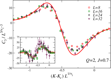
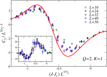
Figure 3: Rescaled $C_{3}$ cumulant along the $J=0.7$ line (top) and the $K=1$ line (bottom) for $Q=2$. Data approach an asymptotic FSS curve, supporting the Ising nature of the transition, although significant scaling corrections are visible for $K=1$. The continuous curves are computed using Eq. (37), with $a=0.67$, $p(ac)^{-3}=2.15$ for $J=0.7$, and with $a=0.78$, $p(ac)^{-3}=0.46$ for $K=1$; the scaling curve ${\cal U}^{(I)}_{3}(X)$ is reported in App. C. In the insets we plot $L^{\omega_{I}}\left[L^{3-3/\nu_{I}}C_{3}(J,K,L)-{\cal C}_{3}(X)\right]$ versus $X$ with $\omega_{I}=0.83$. The observed behavior is consistent with Eq. (39), as expected for a transition in the Ising universality class.

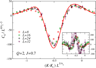
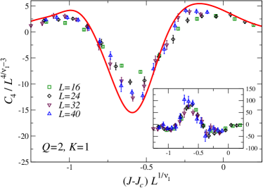
Figure 4: Rescaled $C_{4}$ cumulant along the $J=0.7$ line (top) and the $K=1$ line (bottom) for $Q=2$. The continuous curves are computed using Eq. (37) with $a=0.67$, $p(ac)^{-4}=2.55$ for $J=0.7$, and with $a=0.78$, $p(ac)^{-4}=0.35$ for $K=1$. We use the relation ${\cal U}^{(I)}_{4}(X)=\partial_{X}{\cal U}^{(I)}_{3}(X)$; the scaling function ${\cal U}^{(I)}_{3}(X)$ is reported in App. C. We do not report MC data for $K=1$ and $L=56$ because they are too noisy. In the insets we plot $L^{\omega_{I}}\left[L^{3-4/\nu_{I}}C_{4}(J,K,L)-{\cal C}_{4}(X)\right]$ versus $X$ with $\omega_{I}=0.83$. The observed behavior is consistent with Eq. (39), as expected for a transition in the Ising universality class.

For $Q=2$ we have performed simulations along the line $K=1$ on lattices of size up to $L=56$, and along the line $J=0.7$ on lattices up to $L=32$. MC estimates of $C_{3}$ are shown in Fig. 3. They are consistent with the asymptotic Ising-gauge FSS behavior

$$L^{3-k/\nu_{I}}C_{k}(J,K,L)\approx{\mathcal{C}}_{k}(X),$$ (35)

$$X=(K-K_{c})L^{1/\nu_{I}}\ \mathrm{or}\ X=(J-J_{c})L^{1/\nu_{I}}.$$ (36)

However, we note the presence of significant scaling corrections, in particular, in the data along the $K=1$ line (we will return to this point later). From fits of $C_{3}$ to the scaling behavior (35) fixing $\nu_{I}$ to the Ising value, we obtain $K_{c}(J=0.7)=0.5880(2)$ and $J_{c}(K=1)=0.34910(6)$. The other cumulants give compatible, but less precise, results.

A stronger check that the critical behavior is the same as that of the ${\mathbb{Z}}_{2}$ gauge model is obtained by comparing the computed scaling functions ${\cal C}_{k}(X)$ and the universal curve ${\mathcal{U}}_{k}^{(I)}$ that we have computed for the $\mathbb{Z}_{2}$ gauge model with the same boundary conditions, see App. C. Eq. (24) implies

$$\mathcal{C}_{k}(X)={p\over(ac)^{k}}\,\mathcal{U}_{k}^{(I)}(X/a),$$ (37)

where $p$, $a$, and $c$ are constants that depend on the model but not on the order $k$ of the cumulant. In Fig. 3, we compare the data of the combination $L^{3-3/\nu_{I}}C_{3}$ with the scaling curves $\mathcal{C}_{3}(X)$ obtained from Eq. (37). The normalization constants have been determined to best agreement. We find $a\approx 0.67$ and $p(ac)^{-3}\approx 2.15$ for $J=0.7$, and $a\approx 0.78$ and $p(ac)^{-3}\approx 0.46$ for $K=1$, with a relative uncertainty of approximately 5%. In Fig. 4 we report the results for $C_{4}$, together with the scaling curve obtained by using Eq. (24):

$$\mathcal{C}_{4}(X)={p\over(ac)^{4}}{\mathcal{U}^{\prime}}_{3}^{(I)}(X/a),$$ (38)

where ${\mathcal{U}^{\prime}}_{3}^{(I)}(Y)=\mathrm{d}\,{\mathcal{U}}_{3}^{(I)}(Y)/\mathrm{d}Y$, see Eq. (17). Using the same constant $a$ reported above, and the estimates $p(ac)^{-4}\approx 2.55$ for $J=0.7$, or $p(ac)^{-4}\approx 0.35$ for $K=1$ (the error on such estimates is about 5% and 10%, respectively), the Ising-gauge scaling curves are in reasonable agreement with the numerical data, again confirming the Ising-gauge nature of the transition. The results obtained from the analysis of $C_{3}$ and $C_{4}$ also allow us to determine the two constants $p$ and $c$ separately: $p\approx 1.3$, $c\approx 1.3$ for $J=0.7$ and $p\approx 1.04$, $c\approx 1.7$ for $K=1$.

Another stringent check is obtained by analyzing the deviations of the finite-volume cumulants from the asymptotic Ising FSS curves. At Ising transitions, for $k\geq 3$, one generally expects the presence of corrections vanishing as $L^{-\omega_{I}}$, with $\omega_{I}=0.8297(2)$ KPSV-16 , see Eq. (23). Deviations from the asymptotic curves $\mathcal{C}_{k}(X)$ are thus expected to satisfy the relation

$$L^{\omega_{I}}\left[L^{3-k/\nu_{I}}C_{k}(J,L)-{\cal C}_{k}(X)\right]\approx{\cal C}_{k,\omega}(X),$$ (39)

for $k\geq 3$. Note that the scaling functions ${\cal C}_{k,\omega}(X)$ are also expected to be universal apart from an overall rescaling if one uses $X/a$ as independent variable, where $a$ is the same constant defined in Eq. (37). As shown in the insets of Figs. 3 and 4, both $C_{3}$ and $C_{4}$ data are nicely consistent with Eq. (39) and with the universality (apart from a rescaling) of ${\cal C}_{k,\omega}(X)$ when expressed in terms of $X/a$ (note that $a$ is approximately the same for the data along the two different lines). Eq. (39) does not hold for $C_{2}$, since the leading corrections are due to the analytic background and decay as $L^{-\alpha_{I}/\nu_{I}}$, with $\alpha_{I}/\nu_{I}\approx 0.1747$.

We also note that the value $J_{c}\approx 0.349$ obtained for $K=1$ is close to the asymptotic $K\to\infty$ critical value $J_{XY}\approx 0.227$, indicating that the transition point at $K=1$ is already in a region where the transition line runs almost parallel to the $K$-axis in Fig. 1. In this situation it might be more natural to use the cumulants $C_{J,k}$ of $H_{z}$ instead of the cumulants $C_{k}$ defined in Eq. (12). Estimates of $C_{J,3}$ and $C_{J,4}$ for $K=1$ are reported in Fig. 5, together with the scaling curves obtained using Eq. (33). Since the constant $p$ has already been determined using the cumulants $C_{k}$, only the constant $c_{J}$ can be tuned. If we set $c_{J}=0.97$, we observe a reasonable agreement for both $C_{J,3}$ and $C_{J,4}$. Finally, we analyzed the scaling corrections, considering the combination defined as in Eq. (39). Data scale nicely, see the insets in Fig. 5. Note also that, as predicted by the RG theory, the scaling curves of the finite-volume corrections differ only by a multiplicative nonuniversal factor from those computed using the cumulants $C_{3}$ and $C_{4}$, see the insets of Figs. 3 and 4 for $K=1$.

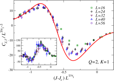
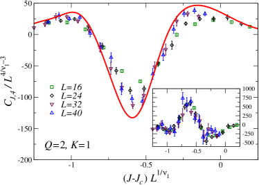
Figure 5: Results for $Q=2$ along the line $K=1$. Rescaled cumulants $C_{J,3}$ (top) and $C_{J,4}$ (bottom), for $Q=2$ along the line $K=1$, using the Ising critical exponent $\nu_{I}=0.629971$. The continuous curves are computed using Eq. (33), with $a=0.78$, $p=1.04$, $c_{J}=0.97$; the scaling curve ${\cal U}^{(I)}_{3}(X)$ is reported in App. C. We do not report estimates of $C_{J,4}$ for $K=1$ and $L=56$ because data are too noisy. In the insets we plot the combination defined as in Eq. (39) versus $X$ with $\omega_{I}=0.83$.

The above results show that the critical behavior of the energy cumulants for $Q=2$ and $K=1$ is fully compatible with the Ising-gauge nature of the transition. They are in apparent contradiction with the numerical analysis of Ref. SSNHS-03 , which reported significant deviations from the Ising behavior in the same region of the phase diagram (see Fig. 7 of Ref. SSNHS-03 , keeping into account that the ratio $\kappa/\beta$ in Ref. SSNHS-03 corresponds to $K/J$ in our notations, thus $\kappa/\beta\approx 2.9$ at the transition point for $K=1$).

We also remark that, with increasing $K$, the regime where the eventual asymptotic FSS behavior can be observed is expected to be pushed toward larger and larger values of $L$, due to the emergence of a preasymptotic regime in which the critical behavior is controlled by the $XY$ spin fixed point. Thus, when the correlation length $\xi$ of the critical modes, or the lattice size $L$ in finite-size systems, is smaller than the crossover length $\xi_{\alpha}\sim K$, we expect to observe an apparent $XY$ critical behavior because the gauge modes are effectively frozen. These preasymptotic crossover effects can be hardly disentangled when performing FSS analyses with data in a limited range of lattice sizes, and may lead to apparent variations of the effective critical exponents with $L$. These crossover effects do not allow us to analyze the critical behavior for values of $K$ significantly larger than 1. For instance, for $K=2$ one would probably need precise results on lattices of size up to $L=100$ to observe the asymptotic behavior with reasonable precision. These simulations would require a huge numerical effort.

In conclusion, the above FSS analyses show that the deconfinement transitions in the $Q=2$ CLAH model are consistent with the expected Ising critical behavior. They belong to the same universality class as the transition in the lattice ${\mathbb{Z}}_{2}$ gauge model. All violations of universality are explained by standard scaling corrections, as predicted by the RG theory of critical phenomena PV-02 . We expect substantial crossover phenomena for large values of $K$, when approaching the $XY$ transition at $K=\infty$, which may be naively interpreted as violations of universality in numerical analyses. Therefore, our results do not confirm the existence of a fixed-point line with varying critical exponents put forward in Ref. SSNHS-03 .

IV.2 Results for $Q=6$

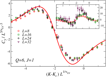
Figure 6: FSS behavior of the third cumulant $C_{3}$ for $Q=6$ along the line $J=1.0$, using the $XY$ critical exponent $\nu_{XY}=0.6717$. We also report (solid curve) the scaling curve (40), obtained by using the parametrization of $\mathcal{U}_{3}^{(XY)}(X)$ reported in App. D. In the inset we plot $L^{\omega_{XY}}\left[L^{3-3/\nu_{XY}}C_{3}(J,L)-{\cal C}_{3}(X)\right]$, with $\nu_{XY}=0.6717$ and $\omega_{XY}=0.789$.

We have performed an analogous FSS analysis of the energy cumulants for $Q=6$ at fixed $J=1.0$. In this case, see the general arguments reported in Sec. II, we expect the deconfinement transitions to belong to the $XY_{G}$ universality class. This is related to the fact that, for $Q>4$, the $J\to\infty$ limit of the model, the lattice ${\mathbb{Z}}_{Q}$ gauge model, undergoes a topological phase transition in the $XY_{G}$ universality class. $XY_{G}$ transitions are expected along the whole transition line, as it occurs in the one-component noncompact lattice AH model BPV-24 .

As already remarked in Sec. III, the behavior of the second cumulant $C_{2}$, which corresponds to the specific heat, is dominated by the analytic background. Therefore, we focus on the third cumulant. Results along the line $J=1.0$ are shown in Fig. 6. They clearly support the expected $XY_{G}$ behavior. The estimates of $L^{3-3/\nu_{XY}}C_{3}$ plotted versus $X=(K-K_{c})L^{1/\nu_{XY}}$ appear to approach a scaling function ${\cal C}_{3}(X)$ if we use the $XY$ value $\nu_{XY}=0.6717$ and $K_{c}\approx 2.0808(4)$. In Fig. 6 we also report (solid curve)

$$\mathcal{C}_{3}(X)={p\over(ac)^{3}}\,\mathcal{U}_{3}^{(XY)}(X/a),$$ (40)

where $a\approx 35$, $p(ac)^{-3}\approx 7.5\cdot 10^{-5}$ (with a relative uncertainty of about 10%), and $\mathcal{U}_{3}^{(XY)}(X)$ is the FSS scaling function of the $XY_{G}$ universality class computed with the same boundary conditions, see App. D. Deviations from the asymptotic curve are expected to scale as in Eq. (39) (with $\nu_{XY}$ replacing $\nu_{I}$). The results, shown in the inset of Fig. 6, are consistent with the $XY_{G}$ nature of the transition. We do not present data for the cumulant $C_{4}$, because the available data are too noisy.

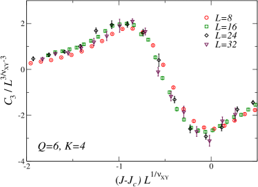
Figure 7: FSS behavior of the third cumulant $C_{3}$ in the $Q=6$ model along the $K=4$ line, with $\nu_{XY}=0.6717$ and $J_{c}=0.4684$.

We also performed some MC simulations along the line $K=4$. We observe a transition at $J_{c}=0.4684(3)$ with exponents consistent with those of the $XY_{G}$ universality class. The scaling curve of $C_{3}$ shows some apparent deviations from the one obtained using Eq. (40), for any choice of the nonuniversal parameters $a$, $p$, and $c$, see Fig. 7. This can be again explained as a crossover effect due to the presence of the unstable spin $XY$ fixed point. Indeed, given that the $XY$ and $XY_{G}$ universality classes differ, we expect the scaling curves computed along the deconfinement line to be unrelated with those computed in the $XY$ spin model with the same boundary conditions (see App. B for a discussion of the appropriate boundary conditions). For large $K$ and finite $L$ we expect data to show a crossover, with an apparent behavior related to that observed in the spin model for small values of $L$ and, more precisely, for $L\ll\xi_{\alpha}$, where $\xi_{\alpha}$ is the crossover length.

To clarify this point we have determined the cumulants in the $XY$ spin model with analogous boundary conditions. Results are shown in Fig. 8. Although significant scaling corrections are present, nevertheless, some qualitative features clearly distinguish the spin $XY$ scaling curve in Fig. 8 from that of the $XY_{G}$ universality class, see Fig. 6. For instance, in the spin $XY$ case the maximum and the minimum are located on opposite sides of the critical point. Instead, they are located on the same side in the $XY_{G}$ case.

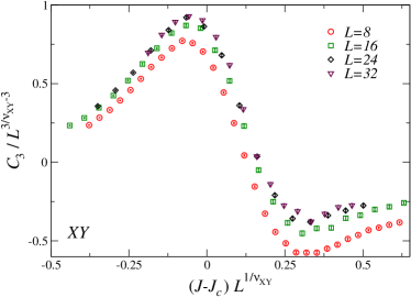
Figure 8: FSS behavior of the third cumulant $C_{3}$ in the $XY$ vector model, with $\nu_{XY}=0.6717$ and $J_{c}=0.22708234$.

The results presented in Fig. 7 show that the FSS behavior of $C_{3}$ at $K=4$ is somewhat intermediate between that expected for the vector $XY$ and for the $XY_{G}$ universality classes. Again, this can be understood by looking at the position of the minimum, which, for $q=6$ and $K=4$ almost coincides with the critical-point position, see Fig. 7. For a quantitative comparison we report the ratio $W_{2}$ defined in Eq. (22): we have $W_{2}\approx 0$ for the $Q=6$ model along the line $K=4$, $W_{2}\approx-0.2$ for the $XY$ model, and $W_{2}=0.25(5)$ for the $XY_{G}$ universality class. We can also compare the ratio $W_{1}$ that is related to the height of the peaks. For this quantity, the $Q=6$ data at $K=4$ are quite different from the $XY$ ones and close to the $XY_{G}$ results. We find $W_{1}\approx-1.5$ for the $Q=6$ model at $K=4$ on the lattices studied, to be compared with $W_{1}\approx-2.4$ and $W_{1}=-1.75(4)$ for the $XY$ ($L=32$ lattice) model and the $XY_{G}$ universality class, respectively.

IV.3 Results for $Q=4$

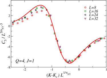
Figure 9: FSS behavior of the third cumulant $C_{3}$ for $Q=4$ along the line $J=1.0$, with $\nu_{XY}=0.6717$, $J_{c}=1.0205$. Data approach the FSS scaling curve computed using Eq. (40); we use the parametrization of $\mathcal{U}_{3}^{(XY)}(X)$ reported in App. D, $a=16$ , $p(ac)^{-3}=9\cdot 10^{-5}$.

Finally, we present some results for $Q=4$. As discussed in Sec. II, this model is expected to represent an exception with respect to the general scenario. Indeed, along the deconfinement line transitions are expected to belong to the $XY_{G}$ and not to the Ising universality class, that characterizes the critical behavior of the lattice ${\mathbb{Z}}_{4}$ model obtained in the $J\to\infty$ limit. This prediction is confirmed by the analysis of the numerical data obtained along the line $J=1$. In Fig. 9 we report a scaling plot of $C_{3}$ using the $XY$ value $\nu_{XY}=0.6717$ and $K_{c}\approx 1.0205(2)$. We also show the scaling curve obtained by using Eq. (40), using the $XY_{G}$ scaling curve with $a=16$ and $p(ac)^{-3}=9\cdot 10^{-5}$ (with a relative uncertainty of about 5%). Data clearly confirm the $XY_{G}$ nature of the transition. We also mention that the MC data are in clear disagreement with the alternative Ising scenario.

V Conclusions

We have investigated the nature of the deconfinement transitions of the one-component multicharge CLAH models defined in Eqs. (1)-(4) (see Fig. 1 for a sketch of the phase diagram). We argue that they belong to the same universality class as the continuous transitions in generic ${\mathbb{Z}}_{Q}$ lattice gauge models without scalar fields. In particular, the transitions belong to the Ising-gauge and $XY_{G}$ universality classes for $Q=2$ and $Q\geq 4$, respectively. For $Q=3$ we expect first-order deconfinement transitions, since there is no universality class with ${\mathbb{Z}}_{3}$ gauge symmetry. This scenario contrasts with the one put forward in Ref. SSNHS-03 , which suggested the existence of a fixed-point line with continuously varying critical exponents.

To accurately investigate the transitions of the single-component model, we consider the FSS behavior of the energy cumulants, see, e.g., Eq. (14). For these quantities we derive several useful general properties that can be used to identify the nature of the critical behavior in any topological transition. We apply these general techniques to the CLAH model with $Q=2,4,6$ for several values of the Hamiltonian parameters.

Our FSS analyses for $Q=2$ indicate that the continuous transitions along the deconfinement transition line belong to the Ising-gauge universality class, i.e., that the critical behavior is the same as in the lattice ${\mathbb{Z}}_{2}$ gauge model, which is formally obtained in the $J\to\infty$ limit. We remark that this check requires a careful analysis of the nonuniversal scaling corrections, which are predicted by the RG approach. Indeed, in FSS analyses of data obtained for relatively small lattices, irrelevant scaling fields or nearby unstable fixed points may give rise to apparent violations of universality. For instance, significant crossover effects (with a crossover length $\xi_{\alpha}\sim K$) are expected for large values of $K$, due to the $XY$ transition occurring for $K=\infty$.

For $Q\geq 4$, the deconfinement transitions should belong to the $XY_{G}$ universality class, with an effective enlargement of the symmetry from ${\mathbb{Z}}_{Q}$ to $U(1)$. This is supported by the FSS analyses of the energy cumulants for $Q=4$ and $Q=6$. Note that for $Q=4$, at variance with what occurs for $Q>4$, the critical behavior along the deconfinement transition line differs from that observed in the ${\mathbb{Z}}_{4}$ gauge model obtain for $J\to\infty$, which instead belongs to the Ising-gauge universality class. Crossover phenomena are expected for large values of $K$ also for $Q\geq 4$. This crossover is quite peculiar as the unstable fixed point is the spin $XY$ fixed point, while the stable one is the gauge $XY_{G}$ fixed point. The two fixed points are different, although related by duality. This implies that, even though critical exponents are the same, other universal properties (for instance, the FSS functions) differ.

We finally mention that, for $Q=3$, the CLAH model is expected to undergo first-order transitions for any finite $K$ and $J$. However, since the continuous $XY$ transition is approached for $K\to\infty$, we expect that the first-order transitions become weaker as $K$ increases. More precisely, the first-order nature becomes apparent only for $L\gg\xi_{\alpha}$, where $\xi_{\alpha}\sim K$ is the crossover length. For smaller sizes, sizable crossover effects are expected, with an apparent $XY$ critical behavior. These crossover effects may explain the results of Ref. SSNHS-03 , which apparently observed a change of the nature of the transition with increasing $K$, from a first-order to a continuous one.

Figure 10: The phase diagram of the $N$-component nCLAH model (58), in the Hamiltonian parameter space $\kappa$-$J$, for $N=1$ (top) and generic $N\geq 2$ (bottom). For $N=1$, there are two phases, the Coulomb (C) and Higgs (H) phases, characterized by the confinement and deconfinement of charged gauge-invariant excitations, respectively. For $N\geq 2$, the scalar field is disordered and gauge correlations are long ranged in the small-$J$ Coulomb (C) phase. For large $J$ two phases occur, the molecular (M) and Higgs (H) ordered phase, in which the global $SU(N)$ symmetry is spontaneously broken. The two phases are distinguished by the behavior of the gauge modes: the gauge field is long ranged in the M phase (small $\kappa$), while it is gapped in the H phase (large $\kappa$). Moreover, while the C and M phases are confined phases, the H phase shows the deconfinement of charged gauge-invariant excitations. See, e.g., Ref. BPV-24 for more details.

It is worth looking at these results in a more general context, considering multicomponent compact and noncompact lattice AH models. To begin with, let us compare the phase diagrams of the one-component ($N=1$) with those of the multicomponent ($N\geq 2$) CLAH models, reported in Figs. 1 and 2, respectively. In the multicomponent model there are three phases, separated by three transition lines. The topological OC-OD transition line, which separates two ordered phases, is the analogue of the deconfinement line in the one-component model. Also in multicomponent models the scalar fields do not directly contribute to the critical behavior along such transition line, which belongs to the ${\mathbb{Z}}_{Q}$ gauge universality class BPV-20-hcAH . The other two lines (DC-OC and DC-OD) are instead associated with the spontaneous breaking of the $SU(N)$ symmetry and are therefore specific of the multicomponent CLAH models. Along, the DC-OC line only scalar fields are critical, and thus the transition is the same as in the $CP^{N-1}$ model. Instead, the DC-OD transitions are driven by a nontrivial interplay between the $U(1)$ gauge and $SU(N)$ global symmetry. For $N<N^{*}$, $N^{*}=7(2)$ these transitions are of first order. For $N\geq N^{*}$ the DC-OD transitions can be continuous, controlled by the stable fixed point of the multicomponent AH field theory BPV-22 ; BPV-20-hcAH .

It is also interesting to compare the phase diagrams of the CLAH models with those of the noncompact lattice AH (nCLAH) models (see App. D for definitions) reported in Fig. 10, which present various phases and transition lines (see, e.g., Refs. BPV-24 ; BPV-21-ncAH for more details). The topology of the phase diagrams is similar both in the one-component and in the multicomponent case. This is not surprising since, as argued in Ref. BPV-22 , the nCLAH models can be obtained as an appropriate large-$Q$ limit of the CLAH models. Interestingly, also the critical behavior in compact and noncompact models is the same, except in one case we discuss below. In multicomponent models the behavior along the CM transition line of the nCLAH model is the same as along the DC-OC line of the CLAH models for any $Q\geq 2$. The same is true for the $Q=1$ multicomponent CLAH models PV-19-AH3d , in which there is a single transition line, which has the same nature as the CM transitions of the nCLAH models and the DC-OC transitions of the multicomponent CLAH models. Analogously, the critical behaviors along the CH line of the nCLAH models and the DC-OD line of the CLAH models for any $Q\geq 2$ (these transitions do not exist for $Q=1$) share the same universality class associated with the stable fixed point of the AH field theory. The deconfinement transitions we have studied here, as well as the OC-OD transitions in multicomponent CLAH models for $Q\geq 4$, belong to the same $XY_{G}$ universality class as the topological transitions in nCLAH models (MH line for $N\geq 2$ and CH line for $N=1$). Only in CLAH systems with charge $Q=2$ these deconfinement transitions belong to a different (Ising-gauge) universality class.

The topological transitions in nCLAH models are associated with the condensation of a nonlocal order parameter defined by dressing the scalar field with a nonlocal electromagnetic cloud KK-85 ; KK-86 ; BN-87 ; BPV-23b ; BPV-24 . The critical correlations of this nonlocal charged operator were numerically studied in Refs BPV-23b ; BPV-24 , exploiting the fact that it assumes a simplified local form in an appropriate Lorenz gauge, where it reduces itself to the scalar-field operator. Along the $XY_{G}$ transition line they display a power-law critical behavior, which definitely differs from that of the local scalar order parameter in standard spin $XY$ transitions, thus providing a better characterization of the $XY_{G}$ universality class. In these studies the use of the Lorenz gauge fixing BPV-23ybq ; BPV-23b was crucial, as the charged order parameter becomes local with this choice of gauge. Since the topological transitions in CLAH models with $Q\geq 4$ have the same critical behavior, it is natural to expect that also these transitions are characterized by the condensation of an appropriately dressed scalar operator or, equivalently, by a local scalar operator in some generalized Lorenz gauge. Such a program is made difficult by the nonlinear nature of the compact gauge fields that does not allow the use of simple linear gauge fixings. A priori one might think of using other gauge fixings, but they may not be appropriate to investigate charged nonlocal excitations; see Refs. BPV-23ybq ; BPV-23b for a discussion. For instance, in the unitary gauge no scalar condensation occurs FMS-81 . If a strategy could be found to overcome these difficulties, it would be possible to investigate charged excitations both for $Q\geq 4$ (it would represent a further universality check) and for $Q=2$.

Appendix A Relation between the $\mathbb{Z}_{4}$ and $\mathbb{Z}_{2}$ gauge models

In this appendix we prove the relation (9) between the partition functions of the $\mathbb{Z}_{4}$ and $\mathbb{Z}_{2}$ gauge models defined by the Hamiltonian (7). For this purpose, it is convenient to expand the partition function as follows

$$Z_{\mathbb{Z}_{Q}}(K)=\sum_{\{\rho\}}e^{-H_{{\mathbb{Z}}_{Q}}(K)}=\sum_{\{\rho\}}\prod_{\mathrm{plaq}}e^{2K\mathrm{Re}\,\Pi_{{\bm{x}},\mu\nu}},\quad$$ (41)

where $\Pi_{{\bm{x}},\mu\nu}=\rho_{{\bm{x}},{\mu}}\,\rho_{{\bm{x}}+\hat{\mu},{\nu}}\,\bar{\rho}_{{\bm{x}}+\hat{\nu},{\mu}}\,\bar{\rho}_{{\bm{x}},{\nu}}$. For $Q=4$ the different values of $\exp(2K\mathrm{Re}\,\Pi_{{\bm{x}},\mu\nu})$, counted with their degeneracies (corresponding to random choices of $\pm 1$ and $\pm i$ on each link), are

$$(Q=4)\quad e^{2K\mathrm{Re}\,\Pi_{{\bm{x}},\mu\nu}}=\left\{\begin{array}[]{ll}e^{2K}&\mathrm{deg}=64\\ 1&\mathrm{deg}=128\\ e^{-2K}&\mathrm{deg}=64\end{array}\right.,$$ (42)

while for $Q=2$ we have

$$(Q=2)\quad e^{2K\mathrm{Re}\,\Pi_{{\bm{x}},\mu\nu}}=\left\{\begin{array}[]{ll}e^{2K}&\mathrm{deg}=8\\ e^{-2K}&\mathrm{deg}=8\end{array}\right.\ .$$ (43)

We can now write $Z_{\mathbb{Z}_{2}}(K/2)^{2}$ as a sum on two independent sets of configurations, and it is easily seen that the possibile values (and the corresponding degeneracies) of the expression $\exp[K(\mathrm{Re}\,\Pi^{(1)}_{{\bm{x}},\mu\nu}+\mathrm{Re}\,\Pi^{(2)}_{{\bm{x}},\mu\nu})]$ are exactly the same as reported in Eq. (42), from which we obtain Eq. (9). We mention that an analogous relation holds for the $\mathbb{Z}_{4}$ and $\mathbb{Z}_{2}$ clock models HS-03 .

Appendix B The role of the boundary conditions in the limiting models

We wish now to discuss the limits $J\to\infty$ and $K\to\infty$ in a finite volume $L^{3}$. We consider both periodic boundary conditions (PBC),

$$\lambda_{{\bm{x}}+L\hat{\mu},\nu}=\lambda_{{\bm{x}},\nu}\qquad z_{{\bm{x}}+L\hat{\mu}}=z_{\bm{x}},$$ (44)

and $C^{*}$ boundary conditions

$$\lambda_{{\bm{x}}+L\hat{\mu},\nu}=\overline{\lambda}_{{\bm{x}},\nu}\qquad z_{{\bm{x}}+L\hat{\mu}}=\bar{z}_{\bm{x}}.$$ (45)

The limit $J\to\infty$ is particularly simple. Indeed, if we start from the unitary-gauge Hamiltonian (5), the increase of $J$ has the only effect of reducing the fluctuations of $\lambda_{{\bm{x}},\mu}$, which, in the limit, takes only $Q$ different values. Therefore, the limiting model has the same boundary conditions considered in the finite-$J$ system.

Let us now discuss the limit $K\to\infty$. In this limit all gauge plaquettes are equal to the identity. For both PBC and $C^{*}$ boundary conditions, we can set, modulo gauge transformations,

$$\lambda_{(x_{1},x_{2},x_{3}),\mu} = V_{1}\quad\hbox{if $x_{1}=L$, $1\leq x_{2},x_{3}\leq L$, $\mu=1$,}$$ (46)

$$= V_{2}\quad\hbox{if $x_{2}=L$, $1\leq x_{1},x_{3}\leq L$, $\mu=2$,}$$

$$= V_{3}\quad\hbox{if $x_{3}=L$, $1\leq x_{1},x_{2}\leq L$, $\mu=3$,}$$

$$= 1\quad\hbox{otherwise},$$

where $V_{1},V_{2},V_{3}$ are three arbitrary phases. We consider here a cubic lattice of size $L^{3}$ and set ${\bm{x}}=(x_{1},x_{2},x_{3})$ with $1\leq x_{\mu}\leq L$.

In the PBC case, the gauge fields given in Eq. (46) satisfy $\Pi_{{\bm{x}},\mu\nu}=1$ on all plaquettes and gauge invariance is completely fixed. The presence of the three phases $V_{\mu}$ is related to the fact that, in the PBC case, a field configuration $\lambda_{{\bm{x}},\mu}$ is completely specified (modulo gauge transformations) not only by the values of the fields on the plaquettes but also by the values of three Polyakov loops (the product of the gauge fields along a straight lattice line that winds around the lattice) in the three different directions. We substitute Eq. (46) in the scalar Hamiltonian and obtain the standard $XY$ vector Hamiltonian except on the boundary links. The boundary terms are

$$-2J\ \sum_{x_{a},x_{b}}\hbox{Re}\Bigl{(}\bar{z}_{(L,x_{a},x_{b})}z_{(1,x_{a},x_{b})}W_{1}+$$ (47)

$$\qquad+\bar{z}_{(x_{a},L,x_{b})}z_{(x_{a},1,x_{b})}W_{2}+\bar{z}_{(x_{a},x_{b},L)}z_{(x_{a},x_{b},1)}W_{3}\Bigr{)},$$

where $W_{\mu}=V_{\mu}^{Q}$. Thus, we obtain an $XY$ spin model with three additional dynamical boundary fields. They are irrelevant in the infinite-volume limit, but change the FSS properties of the model for finite sizes. One can also view the resulting model as a standard $XY$ model with fluctuating boundary conditions, i.e., with fields satisfying

$$z_{{\bm{x}}+L\hat{\mu}}=W_{\mu}z_{\bm{x}}.$$ (48)

In the case of $C^{*}$ boundary conditions, Eq. (46) does not guarantee that $\Pi_{{\bm{x}},\mu\nu}=1$ on all plaquettes. Indeed, there are three additional conditions. If we consider ${\bm{x}}=(L,L,1)$, $\mu=1$ and $\nu=2$, we have

$$\Pi_{{\bm{x}},\mu\nu}=\lambda_{(L,L,1),1}\bar{\lambda}_{(1,L,1),2}\lambda_{(L,1,1),1}\bar{\lambda}_{(L,L,1),2}=V_{1}^{2}\bar{V}_{2}^{2},$$ (49)

which implies $V_{1}^{2}=V_{2}^{2}$, Analogously, we obtain $V_{1}^{2}=V_{3}^{2}$. Therefore, we can set $V_{1}=\sigma_{1}V_{3}$ and $V_{2}=\sigma_{2}V_{3}$, where $\sigma_{1}$ and $\sigma_{2}$ can only take the values $\pm 1$. Substituting the gauge fields in the scalar Hamiltonian, we obtain an $XY$ model with nontrivial boundary terms:

$$-2J\ \sum_{x_{a},x_{b}}\hbox{Re}\Bigl{(}z_{L,x_{a},x_{b}}z_{1,x_{a},x_{b}}\sigma_{1}^{Q}W$$ (50)

$$\qquad+z_{x_{a},L,x_{b}}z_{x_{a},1,x_{b}}\sigma_{2}^{Q}W+z_{x_{a},x_{b},L}z_{x_{a},x_{b},1}W\Bigr{)},$$

where $W=V_{3}^{Q}$. If we now perform a global change of variables $z^{\prime}_{\bm{x}}=W^{1/2}z_{\bm{x}}$, we can get rid of the phase $W$. If $Q$ is even, also the signs $\sigma_{1}$ and $\sigma_{2}$ drop out and thus we obtain an $XY$ spin model with $C^{*}$ boundary conditions. For odd $Q$, instead, we obtain an $XY$ model with ${\mathbb{Z}}_{2}$-fluctuating $C^{*}$ boundary conditions.

These considerations can also be applied to the AH model with ${\mathbb{Z}}_{2}$ gauge and matter fields: $\lambda_{{\bm{x}},\mu}$ and $z_{\bm{x}}$ are real and take only the values $\pm 1$. If we use PBC, for $J\to\infty$ we obtain the ${\mathbb{Z}}_{2}$ lattice gauge model with the same boundary conditions. For $K\to\infty$ we obtain the usual Ising model, but with fluctuating boundary conditions. The ${\mathbb{Z}}_{2}$ scalar fields satisfy $z_{{\bm{x}}+L\hat{\mu}}=V_{\mu}{z}_{\bm{x}}$, where $V_{\mu}=\pm 1$. The latter result allows us to clarify the role of duality in finite-size systems. Ref. BDI-75 showed that the ${\mathbb{Z}}_{2}$ AH model satisfies an exact duality relation for finite $J$ and $K$. The duality relation also holds in a finite cubic volume if PBC are used. By taking the limits $J\to\infty$ or $K\to\infty$, it is easy to see that duality relates the ${\mathbb{Z}}_{2}$ pure gauge model obtained for $J\to\infty$ with the Ising model obtained for $K\to\infty$. This relation also holds in a finite volume, provided one considers the boundary conditions that are obtained by properly performing the two limits. Thus, in a finite cubic volume the ${\mathbb{Z}}_{2}$ pure gauge model with PBC is not exactly dual to the Ising spin model with PBC. Exact duality holds only if one considers the Ising model with fluctuating boundary conditions as discussed above.

Appendix C Energy-cumulant scaling functions in the 3D ${\mathbb{Z}}_{2}$ gauge model

In this section we determine the universal scaling functions $\mathcal{U}_{k}^{(I)}(X)$ for the gauge Ising universality class with periodic boundary conditions ($C^{*}$ and periodic boundary conditions are equivalent for ${\mathbb{Z}}_{2}$ gauge variables). For this purpose we consider the ${\mathbb{Z}}_{2}$ gauge theory and use Eq. (30). We have performed high-precision simulations on lattice up to $L=64$ in the range $-2.0\leq X\leq 0.5$. We have determined the cumulants $\widetilde{C}_{n}(K)$ of $H_{\lambda}$, which are related to the cumulant $C_{n}(K)$ defined in Sec. III by

$$\widetilde{C}_{n}(K,L)={1\over K^{n}}C_{n}(K).$$ (51)

Because of Eq. (30) we have in the scaling limit

$$\widetilde{C}_{n}(K,L)\approx L^{n/\nu-3}{\mathcal{U}}_{n}^{(I)}(X)+\widetilde{b}_{n}(K).$$ (52)

The data for $n=3$ and $4$ scale nicely and allow us to compute the corresponding scaling functions $\mathcal{U}_{n}^{(I)}(X)$, where we have added a superscript ${(I)}$ to specify that the results refer to the Ising gauge universality class with periodic boundary conditions. Data are quite precisely interpolated by the following expression:

$$\mathcal{U}_{3}^{(I)}(X) = -(16399.705+30410.750X+26897.615X^{2}+13094.665X^{3}$$ (53)

$$\quad+3416.983X^{4}+369.113X^{5})\exp[-(X-m_{1})^{2}/(2\sigma_{1}^{2})]$$

$$+(302.042-1329.328X+2523.811X^{2}-2655.760X^{3}$$

$$\quad+1536.383X^{4}-402.120X^{5})\exp[-(X-m_{2})^{2}/(2\sigma_{2}^{2})]$$

where $m_{1}=-1.1$, $m_{2}=-0.3$, $\sigma_{1}=0.38$, and $\sigma_{2}=0.46$. This expression interpolates all data points with $L\geq 32$ with deviations that are of the order of or smaller than the statistical errors (the errors on $\widetilde{C}_{3}(K,L)L^{3-3/\nu_{I}}$ are approximately equal to 0.1 for $L=32,48$ and 0.2 for $L=64$), see the upper panel of Fig. 11. By differentiating $\mathcal{U}_{3}^{(I)}(X)$ with respect to $X$ we obtain the scaling curve $\mathcal{U}_{4}^{(I)}(X)$, which is in very good agreement with the numerical data, see the lower panel of Fig. 11. We can compute the universal RG invariant ratios (22), obtaining

$$W_{1}=-1.59(3)\qquad W_{2}=0.41(4)\qquad W_{3}=0.74(3).$$ (54)

These results hold for any model in the Ising gauge universality class with $C^{*}$/periodic boundary conditions, and can be compared, e.g., with those characteristic of the $XY_{G}$ universality class, see Eq. (62).

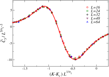
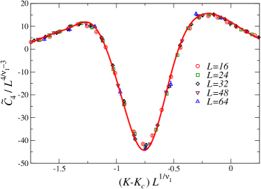
Figure 11: FSS behavior of the energy cumulants $\widetilde{C}_{3}$ (top) and $\widetilde{C}_{4}$ (bottom), for the 3D ${\mathbb{Z}}_{2}$ gauge model. The solid line in the upper panel is the interpolation $\mathcal{U}_{3}^{(I)}(X)$ reported in Eq. (53), while the solid line in the lower panel corresponds to $\frac{\mathrm{d}}{\mathrm{d}X}\mathcal{U}_{3}^{(I)}(X)$.

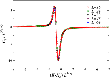
Figure 12: Plot of $\widetilde{B}_{3}(J,L)L^{-3/\nu_{I}+3}$ versus $X$ in the extended range $-8\leq X\leq 9$ and interpolated scaling curve $\mathcal{U}_{3}^{(I)}(X)$

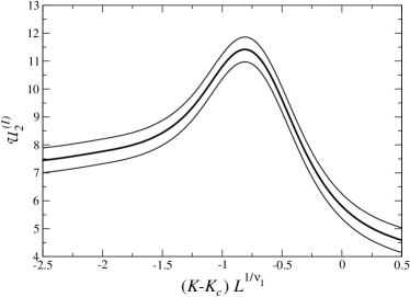
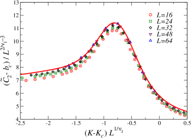
Figure 13: (Top): Plot of the scaling curves $\mathcal{U}_{2a}^{(I)}(X)$ and $\mathcal{U}_{2b}^{(I)}(X)$ (thin lines) and of their average, which is what we consider our best estimate (thick central line). (Bottom): Plot of $(\widetilde{C}_{2}(J,L)-b_{c})L^{-2/\nu_{I}+3}$ with $b_{c}=-4.10$. The thick line is the estimate of $\mathcal{U}_{2}^{(I)}(X)$.

We have also determined the scaling curve $\mathcal{U}_{2}^{(I)}(X)$ for the second moment, using relation (28). For this purpose, however, we need to determine $\mathcal{U}_{3}^{(I)}(X)$ on the whole real axis. In practice, we need simulations in a wider range of values of $X$, such that we are able to observe the asymptotic behavior (26) for large values of $|X|$. Then, if we use a parametrization that satisfies Eq. (26), we expect it to be approximately valid also for large and small values of $X$ outside the simulation interval. We have therefore performed an additional set of simulations on lattices of size $L=24$ in the ranges $-8\leq X\leq-2$ and $0.6\leq X\leq 9$ and determined a new parametrization of the MC data in the whole range $-8\leq X\leq 9$, see Fig. 12. Then, we have computed two different approximations of $\mathcal{U}_{2}^{(I)}(X)$:

$$\mathcal{U}_{2a}^{(I)}(X) = \int_{-\infty}^{X}dY\mathcal{U}_{3}^{(I)}(Y)$$

$$\mathcal{U}_{2b}^{(I)}(X) = -\int_{X}^{\infty}dY\mathcal{U}_{3}^{(I)}(Y).$$ (55)

The difference between the two results allows us to understand the role of the tails of $\mathcal{U}_{3}^{(I)}(X)$. Indeed, for values of $X$ in the simulation interval, the first expression depends on the extrapolation for $X\to-\infty$, but not on the values of $\mathcal{U}_{3}^{(I)}(X)$ for large $X$. Viceversa, the second expression is only sensitive to the large-$X$ extrapolation. The two expressions differ by a constant value, which is approximately equal to 0.9. As our final estimate we consider, see the upper panel of Fig. 13,

$$\mathcal{U}_{2}^{(I)}(X)={1\over 2}[\mathcal{U}_{2a}^{(I)}(X)+\mathcal{U}_{2b}^{(I)}(X)].$$ (56)

We expect the absolute error on this quantity to be approximately $0.9/2\approx 0.5$. In the interval $-2\leq X\leq 0.5$, the curve $\mathcal{U}_{2}^{(I)}(X)$ can be determined using the parametrization (53) and

$$\mathcal{U}_{2}^{(I)}(X)=\mathcal{U}_{2}^{(I)}(0)+\int_{0}^{X}dY\mathcal{U}_{3}^{(I)}(Y),$$ (57)

where $\mathcal{U}_{2}^{(I)}(0)=5.8(4)$.

To compare the estimated $\mathcal{U}_{2}^{(I)}(X)$ with the data, it is necessary to take into account the analytic-background contribution, see Eq. (23). In the scaling limit we can simply replace $b_{2}(J)$ with its value at criticality, i.e., with $b_{c}=b_{2}(J_{c})/K_{c}^{2}$. This constant has been fixed by requiring the MC estimates of $\widetilde{C}_{2}(K,L)$ for $X\approx 0$ and $L\geq 48$ to agree with $\mathcal{U}_{2}^{(I)}(0)L^{2/\nu_{I}-3}+b_{c}$. We obtain $b_{c}=-4.1(9)$, where the error is essentially due to the uncertainty on the scaling curve. Note that background contribution is large and comparable with the scaling contribution [$\mathcal{U}_{2}^{(I)}(0)L^{2/\nu_{I}-3}\approx 11.2$ with an approximate error of 0.9, for $L=48$], which explains why it is not possible to estimate critical exponents from the behavior of $C_{2}$ (the specific heat). In the lower panel of Fig. 13, we compare $\mathcal{U}_{2}^{(I)}(X)$ with the data, observing a reasonable agreement for all values of $X$.

Appendix D Energy-cumulant scaling functions in the inverted $XY$ model

To determine the universal scaling curves ${\cal U}_{k}^{(XY)}(X)$ for the $XY_{G}$ universality class, we should consider an arbitrary model in this universality class and cumulants normalized so that Eq. (17) holds. For this purpose we have considered the inverted $XY$ model DH-81 ; NRR-03 , which can be obtained as the $J\to\infty$ limit of the $N=1$ noncompact LAH model, with Hamiltonian $H=KH_{A}+JH_{z}$, where

$$H_{A} = \frac{1}{2}\sum_{{\bm{x}},\mu>\nu}F_{{\bm{x}},\mu\nu}^{2},$$

$$H_{z} = -2\sum_{{\bm{x}},\mu}{\rm Re}\,(\lambda_{{\bm{x}},\mu}z_{\bm{x}}z_{{\bm{x}}+\hat{\mu}}),$$ (58)

and partition function

$$Z=\int[dA_{{\bm{x}},\mu}d\bar{z}_{\bm{x}}d{z}_{\bm{x}}]e^{-H({\bm{A}},{z})}.$$ (59)

We have defined $\lambda_{{\bm{x}},\mu}=e^{iA_{{\bm{x}},\mu}}$, $F_{{\bm{x}},\mu\nu}=\Delta_{\mu}A_{{\bm{x}},\nu}-\Delta_{\nu}A_{{\bm{x}},\mu}$, $\Delta_{\mu}A_{{\bm{x}},\nu}=A_{{\bm{x}}+\hat{\mu},\nu}-A_{{\bm{x}},\nu}$, and $A_{{\bm{x}},\nu}$ is a real variable. This model is well defined on a finite lattice with $C^{*}$ boundary conditions BPV-21-ncAH .

We perform simulations in the inverted $XY$ model obtained for large values of $J$, determining the third cumulant $\widetilde{C}_{3}$ of $H_{A}$, cf. Eq. (51), for lattices up to $L=32$. Data should scale as

$$\widetilde{C}_{3}(K,L)\approx L^{3/\nu_{XY}-3}{\mathcal{U}}_{n}^{(XY)}(X),$$ (60)

where $X=(K-K_{c})L^{1/\nu_{XY}}$ with $K_{c}=0.076051$ (from Ref. NRR-03 ). The scaling is excellent, see Fig. 14. The results are parametrized by the following function:

$$K_{c}^{3}{\cal U}_{3}^{(XY)}(x)= (104.93856-417.6510x+2172.749x^{2}+72345.33x^{3}+1.4355919\cdot 10^{6}x^{4})e^{-0.5s_{2}(x-\mu)^{2}}$$ (61)

$$-\frac{150.76378+393.6980x+11444.009x^{2}}{1+s_{2}(x-\mu)^{2}}+\frac{598978.55x^{3}+9.81037366\cdot 10^{6}\,x^{4}}{1+s_{4}(x-\mu)^{4}},$$

where $\mu=-0.021$, $\sigma=0.042$, $s_{2}=1/\sigma^{2}$, and $s_{4}=1/\sigma^{4}$. This expression holds for $x$ in the range $[-0.15,0.05]$. It interpolates quite precisely all data, with an absolute error $\lesssim 0.5$, The interpolating curve is also reported in Fig. 14.

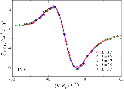
Figure 14: Scaling plot of $\widetilde{C}_{3}$ as a function of $X$ for the inverted $XY$ model. We also report the interpolating curve given in Eq. (61).

Using these data we can also compute the universal RG invariant ratios defined in Eq. (22):

$$W_{1}=-1.75(4)\qquad W_{2}=0.25(5),\qquad W_{3}=0.68(5).$$ (62)

These results can be compared with the analogous results for the $XY$ spin model with the same boundary conditions. The analysis of the data with $L=24$ and 32 gives

$$W_{1}=-2.4(1)\qquad W_{2}=-0.2(1),\qquad W_{3}=0.5(1).$$ (63)

- (1) P. W. Anderson, Basic Notions of Condensed Matter Physics, (The Benjamin/Cummings Publishing Company, Menlo Park, California, 1984).
- (2) X.-G. Wen, Quantum field theory of many-body systems: from the origin of sound to an origin of light and electrons, (Oxford University Press, 2004).
- (3) S. Sachdev, Topological order, emergent gauge fields, and Fermi surface reconstruction, Rep. Prog. Phys. 82, 014001 (2019).
- (4) B. I. Halperin, T. C. Lubensky, and S. K. Ma, First-Order Phase Transitions in Superconductors and Smectic-A Liquid Crystals, Phys. Rev. Lett. 32, 292 (1974).
- (5) E. Fradkin and S. Shenker, Phase diagrams of lattice gauge theories with Higgs fields, Phys. Rev. D 19, 3682 (1979).
- (6) C. Dasgupta and B. I. Halperin, Phase Transitions in a Lattice Model of Superconductivity, Phys. Rev. Lett 47, 1556 (1981).
- (7) J. Fröhlich, G. Morchio, and F. Strocchi, Higgs phenomenon without symmetry breaking order parameter, Nucl. Phys. B190, 553 (1981).
- (8) P. Di Vecchia, A. Holtkamp, R. Musto, F. Nicodemi, and R. Pettorino, Lattice CPN-1 models and their large- behaviour, Nucl. Phys. B 190, 719 (1981).
- (9) G. Bhanot and B. A. Freedman, Finite size scaling for the 3D abelian Higgs model, Nucl. Phys. B 190, 357 (1981).
- (10) D. J. E. Callaway and L. J. Carson, Abelian Higgs model: A Monte Carlo study, Phys. Rev. D 25, 531 (1982).
- (11) J. Bricmont and J. Fröhlich, An order parameter distinguishing between different phases of lattice gauge theories with matter fields, Phys. Lett. 122, 73 (1983).
- (12) K. Fredenhagen and M. Marcu, Charged states in gauge theories, Commun. Math. Phys. 92, 81 (1983).
- (13) T. Kennedy and C. King, Symmetry Breaking in the Lattice Abelian Higgs Model, Phys. Rev. Lett. 55, 776 (1985).
- (14) T. Kennedy and C. King, Spontaneous Symmetry Breakdown in the Abelian Higgs Model, Commun. Math. Phys. 104, 327 (1986).
- (15) C. Borgs and F. Nill, Symmetry Breaking in Landau Gauge A comment to a paper by T. Kennedy and C. King, Commun. Math. Phys. 104, 349 (1986).
- (16) C. Borgs and F. Nill, No Higgs mechanism in scalar lattice QED with strong electromagnetic coupling, Phys. Lett. B 171, 289 (1986).
- (17) C. Borgs and F. Nill, The Phase Diagram of the Abelian Lattice Higgs Model. A Review of Rigorous Results, J. Stat. Phys. 47, 877 (1987).
- (18) N. Read and S. Sachdev, Spin-Peierls, valence-bond solid, and Néel ground states of low-dimensional quantum antiferromagnets, Phys. Rev. B 42, 4568 (1990).
- (19) G. Murthy and S. Sachdev, Actions of hedgehogs instantons in the disordered phase of 2+1 dimensional CPN-1 model, Nucl. Phys. B 344, 557 (1990).
- (20) M. Kiometzis, H. Kleinert, and A. M. J. Schakel, Critical Exponents of the Superconducting Phase Transition, Phys. Rev. Lett. 73, 1975 (1994).
- (21) B. Bergerhoff, F. Freire, D.F. Litim, S. Lola, and C. Wetterich, Phase diagram of superconductors from nonperturbative flow equations, Phys. Rev. B 53, 5734 (1996).
- (22) F. Herbut and Z. Tesanovic, Critical Fluctuations in Superconductors and the Magnetic Field Penetration Depth, Phys. Rev. Lett. 76, 4588 (1996).
- (23) R. Folk and Y. Holovatch, On the critical fluctuations in superconductors, J. Phys. A 29, 3409 (1996).
- (24) V. Yu. Irkhin, A. A. Katanin, and M. I. Katsnelson, expansion for critical exponents of magnetic phase transitions in the model for , Phys. Rev. B 54, 11953 (1996).
- (25) K. Kajantie, M. Karjalainen, M. Laine, and J. Peisa, Masses and phase structure in the Ginzburg-Landau model, Phys. Rev. B 57, 3011 (1998).
- (26) P. Olsson and S. Teitel, Critical Behavior of the Meissner Transition in the Lattice London Superconductor, Phys. Rev. Lett. 80, 1964 (1998).
- (27) C. de Calan and F.S. Nogueira, Scaling critical behavior of superconductors at zero magnetic field, Phys. Rev. B 60, 4255 (1999)
- (28) J. Hove and A. Sudbo, Anomalous Scaling Dimensions and Stable Charged Fixed Point of Type-II Superconductors, Phys. Rev. Lett. 84, 3426 (2000).
- (29) R. D. Sedgewick, D. J. Scalapino, and R. L. Sugar, Fractionalized phase in an gauge model, Phys. Rev. B 65, 054508 (2002).
- (30) T. Senthil and O. Motrunich, Microscopic models for fractionalized phases in strongly correlated systems, Phys. Rev. B 66, 205104 (2002).
- (31) H. Kleinert, F. S. Nogueira, and A. Sudbø, Deconfinement Transition in Three-Dimensional Compact U(1) Gauge Theories Coupled to Matter Fields, Phys. Rev. Lett. 88, 232001 (2002).
- (32) S. Mo, J. Hove, and A. Sudbø, Order of the metal-to-superconductor transition, Phys. Rev. B 65, 104501 (2002).
- (33) A. Sudbø, E. Smørgrav, J. Smiseth, F. S. Nogueira, and J. Hove, Criticality in the (2+1)-Dimensional Compact Higgs Model and Fractionalized Insulators, Phys. Rev. Lett. 89, 226403 (2002).
- (34) J. Smiseth, E. Smørgrav, F. S. Nogueira, J. Hove, and A. Sudbø, Phase Structure of Compact Lattice Gauge Theories and the Transition from Mott Insulator to Fractionalized Insulator, Phys. Rev. B 67, 205104 (2003).
- (35) M. Moshe and J. Zinn-Justin, Quantum field theory in the large limit: A review, Phys. Rep. 385, 69 (2003).
- (36) T. Neuhaus, A. Rajantie, and K. Rummukainen, Numerical study of duality and universality in a frozen superconductor, Phys. Rev. B 67, 014525 (2003).
- (37) T. Senthil, L. Balents, S. Sachdev, A. Vishwanath, and M. P. A. Fisher, Quantum Criticality beyond the Landau-Ginzburg-Wilson Paradigm, Phys. Rev. B 70, 144407 (2004).
- (38) O. I. Motrunich and A. Vishwanath, Emergent photons and transitions in the O(3) -model with hedgehog suppression, Phys. Rev. B 70, 075104 (2004).
- (39) F. S. Nogueira, J. Smiseth, E. Smørgrav, and A. Sudbø, Compact U(1) gauge theories in dimensions and the physics of low dimensional insulating materials, Eur. Phys. J. C 33, 885 (2004).
- (40) J. Smiseth, E. Smorgrav, and A. Sudbø, Critical properties of the -color London model, Phys. Rev. Lett. 93, 077002 (2004).
- (41) S. Takashima, I. Ichinose, and T. Matsui, CP1+U(1) lattice gauge theory in three dimensions: Phase structure, spins, gauge bosons, and instantons, Phys. Rev. B 72, 075112 (2005).
- (42) S. Takashima, I. Ichinose, and T. Matsui, Deconfinement of spinons on critical points: Multiflavor CP1+U(1) lattice gauge theory in three dimension, Phys. Rev. B 73, 075119 (2006).
- (43) S. Wenzel, E. Bittner, W. Janke, A. M. J. Schakel, and A. Schiller, Kertesz Line in the Three-Dimensional Compact U(1) Lattice Higgs Model, Phys. Rev. Lett. 95, 051601 (2005).
- (44) M. N. Chernodub, R. Feldmann, E.-M. Ilgenfritz, and A. Schiller, The compact Abelian Higgs model in the London limit: vortex-monopole chains and the photon propagator, Phys. Rev. D 71, 074502 (2005).
- (45) M. B. Hastings and X.-G. Wen, Quasi-adiabatic Continuation of Quantum States: The Stability of Topological Ground State Degeneracy and Emergent Gauge Invariance, Phys. Rev. B 72, 045141 (2005)
- (46) M. N. Chernodub, E.-M. Ilgenfritz, and A. Schiller, Phase structure of an Abelian two-Higgs model and high temperature superconductors, Phys. Rev. B 73, 100506 (2006).
- (47) A. B. Kuklov, N. V. Prokof’ev, B. V. Svistunov, and M. Troyer, Deconfined criticality, runaway flow in the two-component scalar electrodynamics and weak first-order superfluid-solid transitions, Ann. Phys. 321, 1602 (2006).
- (48) A. W. Sandvik, Evidence for Deconfined Quantum Criticality in a Two-Dimensional Heisenberg Model with Four-Spin Interactions, Phys. Rev. Lett. 98, 227202 (2007).
- (49) I. Herbut, A Modern Approach to Critical Phenomena (Cambridge University Press, 2007).
- (50) R. G. Melko and R. K. Kaul, Scaling in the Fan of an Unconventional Quantum Critical Point, Phys. Rev. Lett. 100, 017203 (2008).
- (51) F. J. Jiang, M. Nyfeler, S. Chandrasekharan, and U. J. Wiese, From an Antiferromagnet to a Valence Bond Solid: Evidence for a First-Order Phase Transition, J. Stat. Mech. (2008) P02009.
- (52) S. Wenzel, E. Bittner, W. Janke, and A. M. J. Schakel, Percolation of Vortices in the 3D Abelian Lattice Higgs Model, Nucl. Phys. B 793, 344 (2008).
- (53) O. I. Motrunich and A. Vishwanath, Comparative study of Higgs transition in one-component and two-component lattice superconductor models, arXiv:0805.1494 [cond-mat.stat-mech].
- (54) A. B. Kuklov, M. Matsumoto, N. V. Prokof’ev, B. V. Svistunov, and M. Troyer, Deconfined Criticality: Generic First-Order Transition in the SU(2) Symmetry Case, Phys. Rev. Lett. 101, 050405 (2008).
- (55) D. Charrier, F. Alet, and P. Pujol, Gauge Theory Picture of an Ordering Transition in a Dimer Model, Phys. Rev. Lett. 101, 167205 (2008).
- (56) R. K. Kaul and S. Sachdev, Quantum criticality of U(1) gauge theories with fermionic and bosonic matter in two spatial dimensions, Phys. Rev. B 77, 155105 (2008).
- (57) T. Ono, S. Doi, Y. Hori, I. Ichinose, and T. Matsui, Phase Structure and Critical Behavior of Multi-Higgs U(1) Lattice Gauge Theory in Three Dimensions, Ann. Phys. (N.Y.) 324, 2453 (2009).
- (58) J. Lou, A. W. Sandvik, and N. Kawashima, Antiferromagnetic to valence-bond-solid transitions in two-dimensional SU(N) Heisenberg models with multispin interactions, Phys. Rev. B 80, 180414 (2009).
- (59) G. Chen, J. Gukelberger, S. Trebst, F. Alet, and L. Balents, Coulomb gas transitions in three-dimensional classical dimer models, Phys. Rev. B 80, 045112 (2009).
- (60) A. W. Sandvik, Continuous Quantum Phase Transition between an Antiferromagnet and a Valence-Bond Solid in Two Dimensions: Evidence for Logarithmic Corrections to Scaling, Phys. Rev. Lett. 104, 177201 (2010).
- (61) D. Charrier and F. Alet, Phase diagram of an extended classical dimer model, Phys. Rev. B 82, 014429 (2010).
- (62) A. Banerjee, K. Damle, and F. Alet, Impurity spin texture at a deconfined quantum critical point, Phys. Rev. B 82, 155139 (2010).
- (63) T. Grover and T. Senthil, Quantum phase transition from an antiferromagnet to a spin liquid in a metal, Phys. Rev. B 81, 205102 (2010).
- (64) S. V. Isakov, R. G. Melko, and M. B. Hastings, Universal signatures of fractionalized quantum critical points, Science 335, 193 (2012).
- (65) R. K. Kaul, Quantum phase transitions in bilayer SU() antiferromagnets, Phys. Rev. B 85, 180411(R) (2012).
- (66) R. K. Kaul and A. W. Sandvik, Lattice Model for the SU() Néel to Valence-Bond Solid Quantum Phase Transition at Large , Phys. Rev. Lett. 108, 137201 (2012).
- (67) K. Harada, T. Suzuki, T. Okubo, H. Matsuo, J. Lou, H. Watanabe, S. Todo, and N. Kawashima, Possibility of Deconfined Criticality in SU() Heisenberg Models at Small , Phys. Rev. B 88, 220408 (2013).
- (68) K. Chen, Y. Huang, Y. Deng, A. B. Kuklov, N. V. Prokof’ev, and B.V. Svistunov, Deconfined Criticality Flow in the Heisenberg Model with Ring-Exchange Interactions, Phys. Rev. Lett. 110, 185701 (2013).
- (69) S. Pujari, K. Damle, and F. Alet, Nèel-State to Valence-Bond-Solid Transition on the Honeycomb Lattice: Evidence for Deconfined Criticality, Phys. Rev. Lett. 111, 087203 (2013).
- (70) M. S. Block, R. G. Melko, and R. K. Kaul, Fate of CPN-1 fixed point with monopoles, Phys. Rev. Lett. 111, 137202 (2013).
- (71) E. V. Herland, T. A. Bojesen, E. Babaev, and A. Sudbø, Phase structure and phase transitions in a three-dimensional SU(2) superconductor, Phys. Rev. B 87, 134503 (2013).
- (72) L. Bartosch, Corrections to scaling in the critical theory of deconfined criticality, Phys. Rev. B 88, 195140 (2013).
- (73) T. A. Bojesen and A. Sudbø, Berry phases, current lattices, and suppression of phase transitions in a lattice gauge theory of quantum antiferromagnets, Phys. Rev. B 88, 094412 (2013).
- (74) A. Nahum, P. Serna, J. T. Chalker, M. Ortuǹo, and A. M. Somoza, Emergent SO(5) Symmetry at the Néel to Valence-Bond-Solid Transition, Phys. Rev. Lett. 115, 267203 (2015).
- (75) A. Nahum, J. T. Chalker, P. Serna, M. Ortuǹo, and A. M. Somoza, Deconfined Quantum Criticality, Scaling Violations, and Classical Loop Models, Phys. Rev. X 5, 041048 (2015).
- (76) G. J. Sreejith and S. Powell, Scaling dimensions of higher-charge monopoles at deconfined critical points, Phys. Rev. B 92, 184413 (2015).
- (77) H. Shao, W. Guo, and A. W. Sandvik, Quantum criticality with two length scales, Science 352, 213 (2016).
- (78) C. Wang, A. Nahum, M. A. Metliski, C. Xu, and T. Senthil, Deconfined Quantum Critical Points: Symmetries and Dualities, Phys. Rev. X 7, 031051 (2017).
- (79) G. Fejos and T. Hatsuda, Renormalization group flows of the -component Abelian Higgs model, Phys. Rev. D 96, 056018 (2017).
- (80) B. Ihrig, N. Zerf, P. Marquard, I. F. Herbut, and M. M. Scherer, Abelian Higgs model at four loops, fixed-point collision and deconfined criticality, Phys. Rev. B 100, 134507 (2019).
- (81) P. Serna and A. Nahum, Emergence and spontaneous breaking of approximate O(4) symmetry at a weakly first-order deconfined phase transition, Phys. Rev. B 99, 195110 (2019).
- (82) A. Pelissetto and E. Vicari, Three-dimensional ferromagnetic CPN-1 models, Phys. Rev. E 100, 022122 (2019).
- (83) A. Pelissetto and E. Vicari, Multicomponent compact Abelian-Higgs lattice models, Phys. Rev. E 100, 042134 (2019).
- (84) A. W. Sandvik and B. Zhao, Consistent scaling exponents at the deconfined quantum-critical point, Chin. Phys. Lett. 37, 057502 (2020).
- (85) A. Pelissetto and E. Vicari, Three-dimensional monopole-free CPN-1 models, Phys. Rev. E 101, 062136 (2020).
- (86) A. Pelissetto and E. Vicari, Large- behavior of three-dimensional lattice CPN-1 models, J. Stat. Mech.: Th. Expt. 033209 (2020).
- (87) C. Bonati, A. Pelissetto, and E. Vicari, Higher-charge three-dimensional compact lattice Abelian-Higgs models, Phys. Rev. E 102, 062151 (2020).
- (88) C. Bonati, A. Pelissetto, and E. Vicari, Lattice Abelian-Higgs model with noncompact gauge fields, Phys. Rev. B 103, 085104 (2021).
- (89) C. Bonati, A. Pelissetto and E. Vicari, Breaking of Gauge Symmetry in Lattice Gauge Theories, Phys. Rev. Lett. 127, 091601 (2021)
- (90) C. Bonati, A. Pelissetto, and E. Vicari, Lattice gauge theories in the presence of a linear gauge-symmetry breaking, Phys. Rev. E 104, 014140 (2021).
- (91) D. Weston and E. Babaev, Composite order in SU(N) theories coupled to an Abelian gauge field, Phys. Rev. B 104, 075116 (2021).
- (92) C. Bonati, A. Pelissetto, and E. Vicari, Three-dimensional monopole-free CPN-1 models: Behavior in the presence of a quartic potential, J. Stat. Mech. (2022) 063206.
- (93) C. Bonati, A. Pelissetto, and E. Vicari, Critical behaviors of lattice U(1) gauge models and three-dimensional Abelian-Higgs gauge field theory, Phys. Rev. B 105, 085112 (2022).
- (94) C. Bonati, A. Pelissetto, and E. Vicari, Scalar gauge-Higgs models with discrete Abelian symmetry group, Phys. Rev. E 105 054132 (2022).
- (95) C. Bonati, A. Pelissetto, and E. Vicari, Coulomb-Higgs phase transition of three-dimensional lattice Abelian Higgs gauge models with noncompact gauge variables and gauge fixing Phys. Rev. E 108, 044125 (2023).
- (96) M. Song, J. Zhao, L. Janssen, M. M. Scherer, and Z. Y. Meng, Deconfined quantum criticality lost, arXiv:2307.02547.
- (97) C. Bonati, A. Pelissetto, and E. Vicari, Abelian Higgs gauge theories with multicomponent scalar fields and multiparameter scalar potentials, Phys. Rev. B 108, 245154 (2023).
- (98) C. Bonati, A. Pelissetto, and E. Vicari, Diverse universality classes of the topological deconfinement transitions of three-dimensional noncompact lattice Abelian-Higgs models, Phys. Rev. D (2024) in press, arXiv:2308.00101.
- (99) R. J. Baxter, Exactly Solved Model in Statistical Mechanics, Academic Press, London, 1982.
- (100) J. Ashkin and E. Teller, Statistics of two-Dimensional lattices with four components, Phys. Rev. 64, 178 (1943).
- (101) L. P. Kadanoff and F. J. Wagner, Some critical properties of the eight-vertex model, Phys. Rev. B. 4, 3989 (1971).
- (102) I. Mukherjee and P. K. Mohanty, Hidden super universality in systems with continuous variation of critical exponents, arXiv:2307.15022.
- (103) J. M. Kosterlitz and D. J. Thouless, Ordering, metastability and phase transitions in two-dimensional systems, J. Phys. C: Solid State 6, 1181 (1973).
- (104) V. L. Berezinskii, Destruction of Long-range Order in One-dimensional and Two-dimensional Systems having a Continuous Symmetry Group I. Classical Systems, Zh. Eksp. Theor. Fiz. 59, 907 (1970) [Sov. Phys. JETP 32, 493 (1971)].
- (105) J. M. Kosterlitz, The critical properties of the two- dimensional xy model, J. Phys. C 7, 1046 (1974).
- (106) J. V. José, L. P. Kadanoff, S. Kirkpatrick, and D. R. Nelson, Renormalization, vortices, and symmetry-breaking perturbations in the two-dimensional planar model, Phys. Rev. B 16, 1217 (1977).
- (107) F. J. Wegner, Duality in Generalized Ising Models and Phase Transitions Without Local Order Parameters, J. Math. Phys. 12, 2259 (1971).
- (108) G. Bhanot and M. Creutz, The Phase Diagram of (n) and (1) Gauge Theories in Three-dimensions, Phys. Rev. D 21, 2892 (1980).
- (109) O. Borisenko, V. Chelnokov, G. Cortese, M. Gravina, A. Papa, and I. Surzhikov, Critical behavior of 3D Z(N) lattice gauge theories at zero temperature, Nucl. Phys. B 879, 80 (2014).
- (110) R. Savit, Duality in Field Theory and Statistical Systems, Rev. Mod. Phys. 52, 453 (1980).
- (111) A. Aharony, Dependence of universal critical behavior on symmetry and range of interaction, in Phase transitions and critical phenomena, vol. 6, p. 357, edited by C. Domb and M. S. Green (Academic Press, London, 1976).
- (112) A. Pelissetto and E. Vicari, Critical Phenomena and Renormalization Group Theory, Phys. Rep. 368, 549 (2002).
- (113) J. Carmona, A. Pelissetto, and E. Vicari, The -component Ginzburg-Landau Hamiltonian with cubic symmetry: a six-loop study, Phys. Rev. B 61, 15136 (2000).
- (114) M. Hasenbusch, Cubic fixed point in three dimensions: Monte Carlo simulations of the model on the lattice, Phys. Rev. B 107, 024409 (2023).
- (115) P. Calabrese, A. Pelissetto, and E. Vicari, Multicritical behavior of -symmetric systems, Phys. Rev. B 67, 054505 (2003).
- (116) M. Hasenbusch and E. Vicari, Anisotropic perturbations in 3D O(N) vector models, Phys. Rev. B 84, 125136 (2011).
- (117) F. Kos, D. Poland, D. Simmons-Duffin, and A. Vichi, Precision islands in the Ising and O() models, J. High Energy Phys. JHEP 08 (2016) 036.
- (118) J. Hove and A. Sudbø, Criticality versus in the (2+1)-dimensional clock model, Phys. Rev. E 68, 046107 (2003).
- (119) A. M. Ferrenberg, J. Xu, and D. P. Landau, Pushing the limits of Monte Carlo simulations for the three-dimensional Ising model, Phys. Rev. E 97, 043301 (2018).
- (120) M. Hasenbusch, Monte Carlo study of an improved clock model in three dimensions, Phys. Rev. B 100, 224517 (2019).
- (121) M. Campostrini, M. Hasenbusch, A. Pelissetto, and E. Vicari, Theoretical estimates of the critical exponents of the superfluid transition in 4He by lattice methods, Phys. Rev. B 74, 144506 (2006).
- (122) Y. Deng, H. W. J. Blöte, and M. P. Nightingale, Surface and bulk transitions in three-dimensional models, Phys. Rev. E 72, 016128 (2005).
- (123) C. Bonati, A. Pelissetto, and E. Vicari, Multicritical point of the three-dimensional Z2 gauge Higgs model, Phys. Rev. B 105, 165138 (2022).
- (124) A. S. Kronfeld and U. J. Wiese, SU(N) gauge theories with C periodic boundary conditions. 1. Topological structure, Nucl. Phys. B 357, 521 (1991).
- (125) B. Lucini, A. Patella, A. Ramos, and N. Tantalo, Charged hadrons in local finite-volume QED+QCD with C∗ boundary conditions, JHEP 02, 076 (2016).
- (126) S. L. Adler, An Overrelaxation Method for the Monte Carlo Evaluation of the Partition Function for Multiquadratic Actions, Phys. Rev. D 23, 2901 (1981)
- (127) N. Metropolis, A. W. Rosenbluth, M. N. Rosenbluth, A. H. Teller, and E. Teller, Equation of state calculations by fast computing machines, J. Chem. Phys. 21, 1087 (1953).
- (128) R. Guida and J. Zinn-Justin, Critical exponents of the -vector model, J. Phys. A 31, 8103 (1998).
- (129) M. Campostrini, A. Pelissetto, P. Rossi, and E. Vicari, 25th order high-temperature expansion results for three- dimensional Ising-like systems on the simple cubic lattice, Phys. Rev. E 65, 066127 (2002).
- (130) M. Hasenbusch, Finite-size scaling study of lattice models in the three-dimensional Ising universality class, Phys. Rev. B 82, 174433 (2010).
- (131) M. V. Kompaniets and E. Panzer, Minimally subtracted six-loop renormalization of -symmetric theory and critical exponents, Phys. Rev. D 96, 036016 (2017).
- (132) M. Hasenbusch, Restoring isotropy in a three-dimensional lattice model: The Ising universality class, Phys. Rev. B 104, 014426 (2021).
- (133) S. M. Chester, W. Landry, J. Liu, D. Poland, D. Simmons-Duffin, N. Su, and A. Vichi, Carving out OPE space and precise O(2) model critical exponents, J. High Energy Phys. 06, 142 (2020).
- (134) C. Bonati, A. Pelissetto and E. Vicari, Gauge fixing and gauge correlations in noncompact Abelian gauge models, Phys. Rev. D 108, 014517 (2023).
- (135) R. Balian, J. M. Drouffe, and C. Itzykson, Gauge fields on a lattice. II. Gauge-invariant Ising model, Phys. Rev. D 11, 2098 (1975).