The SpongeNet Attack: Sponge Weight Poisoning of Deep Neural Networks

Abstract

Sponge attacks aim to increase the energy consumption and computation time of neural networks deployed on hardware accelerators. Existing sponge attacks can be performed during inference via sponge examples or during training via Sponge Poisoning. Sponge examples leverage perturbations added to the model’s input to increase energy and latency, while Sponge Poisoning alters the objective function of a model to induce inference-time energy/latency effects.

In this work, we propose a novel sponge attack called SpongeNet. SpongeNet is the first sponge attack that is performed directly on the parameters of a pre-trained model. Our experiments show that SpongeNet can successfully increase the energy consumption of vision models with fewer samples required than Sponge Poisoning. Our experiments indicate that poisoning defenses are ineffective if not adjusted specifically for the defense against Sponge Poisoning (i.e., they decrease batch normalization bias values). Our work shows that SpongeNet is more effective on StarGAN than the state-of-the-art. Additionally, SpongeNet is stealthier than the previous Sponge Poisoning attack as it does not require significant changes in the victim model’s weights. Our experiments indicate that the SpongeNet attack can be performed even when an attacker has access to only 1% of the entire dataset and reach up to 11% energy increase.

1 Introduction

The wide adoption of deep learning models in production systems introduced a variety of new threats [1]. Most of these threats target the model’s confidentiality and integrity. Evasion attacks [2] alter the model’s input to produce wrong results targeting the model’s integrity. Additionally, backdoor attacks insert a secret functionality into a trained model that can be activated in test time, affecting mostly the model’s integrity [3]. Model stealing [4], membership inference [5], and model inversion [6] attacks extract private information from a trained model violating the victim’s confidentiality. The model’s availability was initially violated by the untargeted poisoning attack that caused a denial of service by significantly decreasing the model’s performance. However, recently a new category of attacks that target the model’s availability has been introduced, the sponge attacks [7, 8, 9, 10]. In sponge attacks, the availability of a model is compromised by increasing latency and energy consumption required for the model to process input. Energy considerations for deep neural networks are highly important. Indeed, numerous papers report that the energy consumption for modern deep neural network models is huge, easily being megawatt hours, see, e.g., [11, 12, 13].

Increasing the models’ latency and energy consumption is possible when neural networks are deployed in application-specific integrated circuit (ASIC) accelerators. ASIC accelerators are used in research and industry to improve the time and cost required to run Deep Neural Networks (DNNs) [14, 15]. More specifically, neural networks are deployed on sparsity-based ASIC accelerators to reduce the amount of computations made during an inference pass. Sponge attacks leverage the reduction of sparsity to eliminate the beneficial effects of ASIC accelerators.

As first shown by Shumailov et al. [7], the availability of models can successfully be reduced through sponge attacks. In particular, language and vision models can be attacked during inference with the introduced sponge examples. Sponge examples are maliciously perturbed images that require more energy for inference than regular samples. They are created [8, 7] in a similar way as adversarial examples for evasion attacks [2]. In particular, Shumailov et al. created their sponge examples with genetic algorithms and L-BFGS for vision models only [7]. For L-BFGS specifically, the magnitude of activations is increased to cause higher energy consumption. Expanding on sponge examples, Cinà et al. [9] introduced the Sponge Poisoning attack. Instead of having the attacker find the optimal sponge perturbation for each sample, Sponge Poisoning allows the attacker to increase the energy consumption at inference by changing a model’s training objective. Additionally, Cinà et al. [9] showed that increasing the magnitude ($\ell_{2}$ norm) of activations, as done with sponge examples, does not maximize the number of firing neurons. Instead, directly using the number of non-zero activations, also called the $\ell_{0}$ norm, in the objective increases the energy consumption more than using the magnitude of activations ($\ell_{2}$).

The attack formulated by Cinà et al. [9] has limitations and has only been tested on vision models. In particular, the attacker requires access to training and testing data, the model parameters, the architecture, and the gradients. The attacker is also required to train the entire model from scratch. However, requiring full access to an entire training procedure and training from scratch can be impractical. Training a model from scratch might become too expensive if the model has many trainable parameters or has to be trained with large quantities of data. To evaluate the practicality of Sponge Poisoning with complex models and large quantities of data, we apply the attack to a GAN. We show that Sponge Poisoning can become much more expensive than our attack when the GAN needs to be trained from scratch (especially with hyperparameter tuning) without guaranteeing better results. To overcome the limitations of Sponge Poisoning, we propose a novel sponge attack called SpongeNet. SpongeNet directly alters the parameters of a pre-trained model instead of the data or the training procedure. The attack compromises the model between training and inference time. SpongeNet can be performed only by accessing the model’s parameters and a small subset of the dataset. In particular, it is effective even when the attacker has access to no more than 10% of the dataset. We show the applicability of our attack on three vision models and four datasets and one GAN on another dataset.

Our main contributions are:

• We introduce the SpongeNet attack. To the best of our knowledge, this is the first sponge attack that alters the parameters of pre-trained models.

• We are first to explore energy attacks on GANs. Both Sponge Poisoning and SpongeNet on a GAN can be done without significant perceivable differences in generation performance.

• We show that the SpongeNet attack effectively increases energy consumption (up to 11%) on a range of vision and generative models and different datasets. Even more importantly, the SpongeNet attack is stealthy, which we consider the primary requirement for sponge attacks. Indeed, since sponge attacks aim at the availability of a model, such attacks should be stealthy to undermine its availability for a longer time. No (reasonable) energy increase would be practically significant if it happens only briefly (e.g., in an extreme case, for one inference).

• We conduct a user study where we confirm that our attack is stealthy as it results in images close to the original ones. More precisely, in 87% of cases, users find the images from SpongeNet closer to the original than those obtained after Sponge Poisoning.

• We are the first to consider parameter perturbations and fine pruning [16] as defenses against sponge attacks. Additionally, we propose adapted variations of these defenses that are applied to the biases of targeted layers instead of the weights of convolutional layers. The regular defenses cannot mitigate the effects of both SpongeNet and Sponge Poisoning, whereas the adapted defenses can reverse the energy increase of both attacks for some models and datasets. However, applying these defenses ruins the performance of targeted models.

Our work focuses on energy consumption increase and not latency since latency is more difficult to measure precisely[7]. Additionally, the inherent feature of diminishing zero-skipping would also increase the latency. Indeed, by default, fewer zeros mean less zero skipping, which means more computations during an inference, translating to more computation time. We provide our code in an anonymous repository.

This paper is organized as follows. In Section 2, we provide background information. Section 3 gives details about our threat model and the SpongeNet attack. Section 4 provides information about the experimental setup, while Section 5 gives experimental results and discussion. Section 6 discusses related works, and finally, in Section 7, we conclude the paper. We also provide Appendices A to D with further experimental results.

2 Background

This section provides background information about sparsity-based ASIC accelerators, sponge attacks, ways to measure energy consumption, and deep neural networks.

2.1 Sparsity-based ASIC Accelerators

Sparsity-based ASIC accelerators reduce the latency and computation costs of running neural network models by using zero-skipping [17, 18, 19]. Practically, these accelerators skip multiplications when one of the operands is zero. This means the overall number of arithmetic operations required to process the inputs and the number of memory accesses are reduced, improving latency and decreasing energy consumption [20]. Many types of DNN architectures with sparse activations, i.e., many zeros, benefit from using these accelerators [21]. The sparsity in DNNs used in our experiments is primarily introduced by the rectified linear unit (ReLU). The ReLU layer allows DNNs to approximate nonlinear functions and is defined as

$$f(x)=max(x,0).$$ (1)

Thus, any negative or zero input to the ReLU is skipped by the ASIC accelerator. Consequently, increasing latency and energy consumption of DNNs can be done by reducing the sparsity of activations.

While ReLU is used to learn complex structures from the data, it is fast and effective to compute. Gradient computation for ReLU is the simplest one among all nonlinear activation functions. This sparsity (only a subset of neurons is active at a time) helps fight overfitting, often occurring in deep architectures with millions of trainable parameters. ReLU, and its sparsity properties, are well-known and widely used, see, e.g., [22, 23, 24, 25, 26]. While the latest neural networks, like transformers, also use different activation functions, research supports that even there, ReLU is an excellent choice [27]. Finally, we note that large, sparsely activated DNNs can consume less than $1/10$th the energy of large, dense DNNs without sacrificing accuracy despite using as many or even more parameters [13].

2.2 Sponge Poisoning

Sponge poisoning is applied at training time, and it alters the objective function [9, 28, 10]. For a certain percentage of the training samples, it will include an extra loss, called sponge loss, to the classification loss. The classification loss is minimized, and the sponge loss is maximized, so the altered objective function is formulated as follows:

$$G_{sponge}(\theta,x,y)=L(\theta,x,y)-\lambda E(\theta,x).$$ (2)

In Eq. (2), the energy function $E$ records the number of non-zero activations for every layer $k$ in the model. The parameter $\lambda$ influences the importance of increasing the energy consumption weighed against the classification loss. The energy function $E$ to record the number of non-zero activations is formulated as:

$$E(\theta,x)=\sum_{k=1}^{K}\hat{\ell_{0}}(\boldsymbol{\phi}_{k}).$$ (3)

In Eq. (3), the number of non-zero activations for a layer $k$ is calculated with an approximation $\hat{\ell_{0}}(\boldsymbol{\phi}_{k})$. This approximation is needed as the $\ell_{0}$ norm is a non-convex and discontinuous function for which optimization is NP-hard [29]. We use the approximation defined and used by [30, 9]:

$$\hat{\ell_{0}}(\boldsymbol{\phi}_{k})=\sum_{j=1}^{d_{k}}\frac{\phi^{2}_{kj}}{\phi^{2}_{kj}+\sigma},$$ (4)

where $\phi_{kj}$ are the output activation values of layer $k$ at dimension $j$ of the model and $d_{k}$ the dimensions of layer $k$.

2.3 Measuring Energy Consumption

In our work, we consider a sparsity-based ASIC accelerator that uses zero-skipping. To calculate the energy consumption of models, we use an ASIC accelerator simulator that employs zero-skipping provided by Shumailov et al. [7]. The simulator estimates the energy consumption of one inference pass of a model by recording the overall number of arithmetic operations and the number of memory accesses to the GPU DRAM required to process the input. The energy consumption is calculated as the amount of energy in Joules it costs to perform operations and memory accesses. Using the simulator, we can measure sponge effects by calculating and comparing the energy consumption of normal and targeted models. We extended the simulator from Shumailov et al. [7] to accommodate, for instance, normalization layers and Tanh activation functions used in StarGAN because the original version did not support these layers.

The energy is estimated by the simulator as a total for all input samples in the given batch. A larger batch size returns a larger energy estimate for the model. Thus, if we use the number of Joules to compare sponge effectiveness between experiments with the same model architecture, we must ensure all batch sizes are the same. Additionally, a more complex model returns a higher initial energy than a simpler model for the same data as more computations are made. This means the increase in Joules does not reflect the sponge attack’s effectiveness between different types of models.

To measure the effectiveness of sponge attacks between different types of models, we use the energy gap [7, 9, 10, 28]. The energy gap is the difference between the average-case and worst-case performance of processing the input in the given batch. It is represented with a ratio between the estimated energy of processing the input on an ASIC optimized for sparse matrix multiplication (average-case) and an ASIC without such optimizations (worst-case). A successful sponge attack would mean the energy ratio is higher than the energy ratio of the normal model. If the ratio approaches 1, the model is close to the worst-case scenario. Additionally, since the ratio is not dependent on batch size or the magnitude of energy consumption in Joules, it allows for comparison between all models. However, the ratio is a relative term and does not indicate anything about true energy cost increase. A targeted model may have less energy ratio increase for dataset A than dataset B, but dataset B might consume more energy in Joules per ratio percentage point.

2.4 GANs

Generative Adversarial Networks (GANs) are a powerful class of neural networks used for unsupervised learning. GANs comprise two neural networks: a discriminator and a generator. They use adversarial training to produce artificial data identical to actual data. Many popular image translation approaches such as cGAN [31], CycleGAN [32], and StarGAN [33] utilize a combination of loss terms in the objective functions to train the generator and discriminator components. Of these, StarGAN [33] is the most successful, as it can learn multiple attribute translations with only one model. The authors use a combination of three loss terms. First, to make the generated images as real as possible, they adopt an adversarial loss $L_{adv}$ that represents the discriminator’s ability to distinguish the generated images. Second, both components contain a domain classification loss. For the generator component, the classification loss $\lambda_{cls}L^{f}_{cls}$ of the generated sample needs to be minimized to produce realistic images. For the discriminator component, the classification loss $\lambda_{cls}L^{r}_{cls}$ for real images and their real attributes needs to be minimized such that the discriminator learns good feature representations of real images. Third, the reconstruction loss $L_{rec}$ is used to train the generator only to change the specified attribute while preserving the rest of the image. The $L_{rec}$ is minimized and calculated by first generating a fake image and subsequently using the generator again to reconstruct the fake image back to its original class. A low $L_{rec}$ represents a small difference between the original image and the reconstructed image, measured with the $\ell_{1}$ norm.

2.5 SSIM

Wang et al. proposed a measure called structural similarity index (SSIM) that compares local patterns of pixel intensities [34]. SSIM computes the changes between two windows:

$$SSIM(x,\hat{x})=\frac{(2\mu_{x}\mu_{\hat{x}}+c_{1})(2\sigma_{x\hat{x}}+c_{2})}{(\mu_{x}^{2}+\mu_{\hat{x}}^{2}+c_{1})(\sigma_{x}^{2}+\sigma_{\hat{x}}^{2}+c_{2})},$$

where $\mu_{x}$ is the pixel sample mean of $x$, $\mu_{\hat{x}}$ is the pixel sample mean of $\hat{x}$, and $c_{1}$ and $c_{2}$ are two variables to stabilize the division, $\sigma_{x}$ is the variance of $x$, $\sigma_{\hat{x}}$ is the variance of $\hat{x}$, and $\sigma_{x\hat{x}}$ is the covariance of $x$ and $\hat{x}$.

3 Methodology

In this section, we first provide details about the threat model we follow. Afterward, we describe the SpongeNet attack.

3.1 Threat model

Knowledge & Capabilities. SpongeNet alters a victim model’s parameters instead of the model’s architecture (like Sponge Poisoning). We assume a white-box setup where the adversary has the full knowledge of the victim model’s architecture and its parameters $\theta$. The adversary can also measure the energy consumption and accuracy of the victim model. Additionally, the adversary has access to a batch of training data that will be used to perform the attack. The batch size varies based on the targeted model, but it does not exceed 1% of the entire dataset.

Attack Goal. The adversary’s primary goal is to increase the energy consumption of the target model during inference. The target model should still perform as well as possible on its designated task. Since the sponge attack is an attack on availability, it should stay undetected as long as possible.

Aligned with the current literature [35], the SpongeNet attack is realistic in the following scenarios:

• A victim, having access to limited resources only, outsources training to a malicious third party who poisons a model before returning it to the end user. The attacked model is trained from scratch, or the adversary uses a pre-trained model.

• An adversary uploads a poisoned model to hosting services such as Microsoft Azure or Google Cloud, causing an increase in energy costs when users use it in their applications.

• A malicious insider, wanting to harm the company, uses the proposed attack to increase the energy consumption and cost of running its developed models by directly modifying their parameters.

3.2 SpongeNet Description

This work proposes a novel sponge attack called SpongeNet. Instead of creating the sponge effect by altering the input (sponge examples) [7, 8] or the objective function (Sponge Poisoning) [10, 9], we directly alter the biases of a trained model. The core idea is to increase the number of positive values used as input to layers such as ReLU, max pooling, and average pooling. Our attack increases energy consumption by reducing the sparsity of activations, introducing fewer possibilities for zero-skipping than in an unaltered model.

Two assumptions are crucial for SpongeNet. First, we assume there are neurons in the model that can be altered without any or much negative effect on the model’s accuracy. This has already been demonstrated in previous works [35], and we also observe it in our experiments. Moreover, this is well-aligned with the Lottery Ticket Hypothesis [36]. If no neurons can be altered, we cannot introduce the sponge effect. Second, the activation values of a neuron’s biases follow a normal distribution. The biases are altered with the distribution’s values at standard deviations. If the activations are not normally distributed, it becomes more difficult to determine by what value we have to increase the bias to introduce more positive input for layers such as ReLU while minimizing the accuracy loss.

If the network uses activation functions that do not promote sparsity, then it cannot benefit from the zero-skipping of sparsity ASICs in these specific layers. Thus, the activation function will already have increased energy consumption. In our experiments, we concentrate on ReLU layers. To verify this, we showed that the potential energy increase would be insignificant if we swapped ReLU with LeakyReLU, as seen in Table 7. Note that we could have chosen models with different activation functions, but ReLU is very popular, making it a very good candidate for our attack.

Our attack consists of five steps:

• Step 1: Identify layers that introduce sparsity. The first step is to identify the layers that introduce sparsity in the model’s activation values. In our experiments, these are the ReLU and any pooling layers. If pooling layers directly follow ReLU layers, then only the ReLU layers need to be considered, as the zeros introduced by the attack in the ReLU layers will also affect the pooling layers.

• Step 2: Create the set of target layers. After identifying the layers that introduce sparsity, we create a subset of these layers that we call the target layers. The target layers are all the layers directly preceding the sparsity layers. These are our target layers because they form the input to the sparsity layers. Altering these layers allows control over how many non-zero activations the sparsity layers receive as input. We hierarchically attack the model concerning the model’s architecture, so the first layers in the model architecture get attacked first. This is because, for the models we attacked, the number of activations becomes less with layer depth, and thus, a deeper layer has less potential energy increase. Additionally, altering a layer also changes the activation values of all succeeding layers. Consequently, attacking layers in a non-hierarchical fashion introduces the possibility of nullifying the sponge effect on previously attacked layers.

• Step 3: Profile activation value distributions of the target layers. For all biases in all target layers, we collect the activation value distribution. The activation distributions that are collected are produced by one inference pass through the clean model with a subset of the validation data.

• Step 4: Calculate the mean and standard deviation of the biases. For each activation distribution of each bias parameter $b$ in target layer $k$, we calculate the mean $\mu_{kb}$ and standard deviation $\sigma_{kb}$. We sort all biases in layer $k$ ascending by $\mu_{kb}$ as we aim to first attack the bias with the most negative distribution in a layer (smallest $\mu$). A small $\mu_{kb}$ indicates that the bias parameter introduces many negative values and zeros in the succeeding ReLU layer. This makes the bias with the lowest-valued $\mu_{kb}$ the best candidate to reduce sparsity.

• Step 5: Alter biases. Using $\mu_{kb}$ and $\sigma_{kb}$, we calculate how much we need to increase bias $b$ to turn a certain percentage of activations in the succeeding ReLU layer positive. We increase the targeted bias $b$ by $\alpha\cdot\sigma_{kb}$. Here, $\alpha$ is a parameter and determines the value by how many standard deviations we increase $b$ in each iteration. Subsequently, we check if the change affects the model’s accuracy beyond the specified accuracy threshold or decreases energy consumption. If yes, we revert the bias parameter to the previous value. If not, we again increase the bias by $\alpha$ and check if the accuracy threshold is exceeded. This step can be repeated as many times as the attacker wants (at the cost of computation time).

4 Experimental Setup

In this section, we describe our experimental setup. First, we discuss the implementation details of the Sponge Poisoning attack on StarGAN, and then we provide the implementation details of our attack. Finally, we discuss the defense setup and the environment specifications.

4.1 Sponge Poisoning

Models and Datasets. We evaluate the Sponge Poisoning attack on a diverse range of architectures and datasets to test the effectiveness of the attack on data with different dimensionality and distributions. We consider ResNet18 [37] and VGG16 [38] models trained on MNIST [39], CIFAR10 [40], GTSRB [41], and TinyImageNet (TIN) [42]. Moreover, we use StarGAN trained on the CelebFaces Attributes (CelebA) dataset [43].

The vision models are trained until convergence with an SGD optimizer with momentum 0.9, weight decay 5e-4, batch size 512, and optimizing the cross-entropy loss. These training settings were chosen because they produce well-performing classification models and are in line with the models trained in the Sponge Poisoning paper [9]. The learning rates for MNIST, CIFAR10, and GTSRB are set to $0.01$, $0.1$, and $0.1$, respectively. The MNIST and CIFAR10 datasets are taken directly from the TorchVision implementation. MNIST has 60 000 training images and 10 000 testing images. CIFAR10 has 50 000 training images and 10 000 testing images. We compose GTSRB with a special split of 39 209 training images and 12 630 testing images, as done in previous work with this dataset for good performance [9, 41]. We set the Sponge Poisoning parameters [9] to $\lambda=2.5$, $\sigma=1e-4$, and $p=0.05$. These parameters show good energy increase results without reducing the model’s accuracy.

Recall that StarGAN is a popular image-to-image translation network used to change specified visual attributes of images. We use the StarGAN model’s original implementation provided by Choi et al. [33]. To apply Sponge Poisoning to StarGAN, we adapt Eq. (2), and instead of the regular classification loss, we use the loss described in Section 2. The StarGAN minimization objective during training is formulated as follows:

$$G_{gen}(\theta,x)=L_{adv}+\lambda_{cls}L^{f}_{cls}+\lambda_{rec}L_{rec}-\lambda E(\theta,x,y).$$ (5)

The CelebA dataset consists of 200 599 training images and 2 000 test images. Each image consists of 40 binary attribute labels. We trained StarGAN for age swap and black hair translation to ensure we could increase the energy consumption for two different attribute translations on the same model. Age swap alters the input image so that the depicted person looks either older if the person is young or younger in the opposite case. Black hair translation changes the color of the person’s hair to black.

Each image in the original dataset is $178\times 218$ pixels. We perform the recommended StarGAN CelebA augmentations [33]. In particular, each image is horizontally flipped with a 0.5 chance, center-cropped at 178 pixels, and resized to 128 pixels. Normalization is applied to each image with mean $\mu=0.5$ and standard deviation $\sigma=0.5$. The same augmentations are applied to the validation set except for horizontal flipping because the generated images should not be flipped when performing visual comparison in the validation phase.

To produce the results for GAN Sponge Poisoning, we choose the parameters $\lambda=2.5$, $\sigma=1e-4$, and $p=0.05$ for the Sponge Poisoning algorithm [9]. These values showed the maximum energy increase without losing generation quality (below SSIM 0.8). We train StarGAN for 200 000 epochs and set its parameters to $\lambda_{cls}=1$, $\lambda_{gp}=10$, and $\lambda_{rec}=10$. We set the learning rate for the generator and discriminator to $0.0001$ and use Adam optimizer with $\beta_{1}=0.5$ and $\beta_{2}=0.999$ and train batch size 8. These parameter values are used for all ablation variations as they are recommended for StarGAN [33].

The effectiveness of Sponge Poisoning is measured with the mean energy ratio per batch over the entire validation set with a batch size of 32. This mean energy ratio of a sponged model is compared to the mean energy ratio of a cleanly trained StarGAN model with the same parameter specifications. Accuracy for the sponge-poisoned versions of StarGAN is reported with a metric often used in GAN literature [44, 45, 46, 47]: the mean SSIM [48]. We calculate the mean SSIM between images generated with a regularly trained StarGAN and images generated by sponged versions of StarGAN. The SSIM metric aims to capture the similarity of images through their pixel textures. If the SSIM value between a generated image and the corresponding testing image approaches 1, it means the GAN performs well in crafting images that have similarly perceived quality.

4.2 SpongeNet

Models and Datasets. Our SpongeNet attack is evaluated on various architectures and data. For vision models, we consider ResNet18 [37] and VGG16 [38] trained on MNIST [39], CIFAR10 [40], GTSRB [41], and TinyImageNet [42]. Additionally, we consider the same StarGAN model with the CelebA faces dataset on which we performed Sponge Poisoning. To get the clean model that we can perform our attack on, we trained StarGAN for 200 000 epochs with $\lambda_{cls}=1$, $\lambda_{gp}=10$, $\lambda_{rec}=10$, and a learning rate of $0.0001$ for the generator and the discriminator. We used Adam optimizer with $\beta_{1}=0.5$ and $\beta_{2}=0.999$, and a train batch size of $8$.

Ablation study. To demonstrate the sponge capabilities of our proposed attack, we perform an ablation study on the threshold parameter specified in Step 4 of the SpongeNet attack procedure. The goal of this ablation parameter is to give an expectation of how much accuracy an attacker needs to sacrifice for a worthwhile energy increase. The considered thresholds for the vision models are 0%, 1%, 2%, and 5%. In general, an adversary would aim for 1) a minimal performance drop on the targeted model so that the attack remains stealthy and 2) as many victims as possible that use it for as long as possible. For this reason, we chose a maximum threshold of 5% to set an upper bound for the attack’s performance. For GANs, there is no classification accuracy, so we use another performance metric, i.e., SSIM (as discussed in Section 4.1).

The effectiveness of SpongeNet is measured with the mean energy ratio per batch over the entire validation set, with a batch size of 512 for all vision models and a batch size of 32 for StarGAN. The performance of all attacked vision models is measured using the accuracy on the validation set. The generation performance of SpongeNet versions of StarGAN is reported with the mean SSIM per image compared to the images generated with a regularly trained StarGAN.

4.3 Defenses

As fine-tuning the model with the inverse of the Sponge Poisoning algorithm (model-sanitization) is shown to be overly costly to mitigate the effects of Sponge Poisoning [9], we consider another two methods that are used as defenses against poisoning: parameter perturbations and fine-pruning [16]. These defenses are evaluated against both Sponge Poisoning and SpongeNet.

Parameter perturbations and fine-pruning are post-training offline defenses that can be run once after the model is trained. Thus, they are not run in parallel with the model, which could lead to a constant increase in the model’s energy consumption. Typically, these defenses are applied to the convolutional layers’ weights [16]. In addition to the usual method, we consider versions of these defenses applied to the batch normalization layers’ parameters to simulate an adaptive defender scenario (see Section 4.3).

Parameter perturbations. In our experiments, we consider two types of parameter perturbations: random noise addition and clipping. When attackers perform Sponge Poisoning or SpongeNet, they increase the model’s parameter values. By adding random negative valued noise to the model’s parameters, a defender aims to lower parameter values and reduce the number of positive activation values caused by Sponge Poisoning or SpongeNet. The random noise added is taken from a standard Gaussian distribution because, as stated in [35] “DNNs are resilient to random noises applied to their parameter distributions while backdoors injected through small perturbations are not". We believe that through SpongeNet and Sponge Poisoning, we inject small perturbations similar to the backdoors into the models, which is worth exploring experimentally. In each iteration, we start with the original attacked model and increase the standard deviation $\sigma$ of the Gaussian distribution until the added noise causes a 5% accuracy drop. Since the noise is random, we perform noise addition five times for every $\sigma$ and report the average energy ratio and accuracy.

Using clipping has the same purpose as adding noise. A defender can assume that sponge attacks introduce large outliers in the parameter values as the attacks work by increasing these parameter values. Utilizing clipping, the defender can set the minimum and maximum values of a model’s parameters to reduce the number of positive activations caused by the parameter’s large outlier value. We apply clipping by setting all parameters in a layer to that layer’s minimum and maximum parameter values multiplied by a value between 0 and 1. We start with 1 and reduce the multiplication value in every iteration. Every iteration starts with the original parameter values. We clip the values until there is a 5% accuracy drop.

Fine-pruning. Fine-pruning is a defense designed to mitigate or even reverse the effects introduced by poisoning attacks [16]. The defense is a combination of pruning and fine-tuning. The first step is to set a number of parameters in the layer to 0 (pruning), and then the model is re-trained for a number of epochs (fine-tuning) to reverse the manipulations made to the parameters. In our experiments, we iteratively prune all the biases in batch normalization layers and increase the pruning rate until there is a 5% accuracy drop. Subsequently, we retrain the vision models for 5 epochs and StarGAN for 5 000 epochs; these represent 5% of the total number of training epochs for the vision models and StarGAN, respectively. Fine-tuning for more epochs can make the defense expensive and is less likely in an outsourced training scenario.

Adaptive Defender Scenario

Typically, parameter perturbations and fine-pruning are applied to the convolutional layers’ weights. In addition to the usual method, we adapt the parameter perturbation defenses to target the parameters affected by SpongeNet. The adaptive defender knows how the sponge attacks work and is specifically defending against them and, as such, tries to minimize the batch normalization layers’ biases. Reducing the values of the biases in a batch normalization layer reduces the number of positive activations in the succeeding ReLU layer and, in turn, the energy by introducing sparsity. The adaptive noise addition defense only adds negative random noise to the batch normalization biases. By only adding negative random noise, we reduce the bias values. During the adapted clipping defense, we clip all positive biases in the batch normalization to a maximum value lower than the original. Clipping the biases lowers the values of large biases exceeding the maximum and thus reduces the number of positive activations that go to the succeeding ReLU layer. For fine-pruning, we only consider the adaptive defender scenario as, typically, fine-pruning [16] is applied on the last convolutional layer. Pruning the last convolutional layer will have no effect, as the energy increases happen in the preceding layers. We prune only the positive biases because pruning negative biases to zero will increase the value and potentially cause more positive activations in succeeding layers.

4.4 Environment and System Specification

We run our experiments on an Ubuntu 22.04.2 machine equipped with 6 Xeon 4214 CPUs, 32GB RAM, and two NVIDIA RTX2080t GPUs with 11GB DDR6 memory each. The code for the neural networks is developed with PyTorch 2.1.

5 Experimental Results

In this section, we provide the experimental results for SpongeNet and a comparison to the Sponge Poisoning attack [9]. Afterward, we conduct an ablation study for SpongeNet’s parameters. Next, we evaluate both SpongeNet and Sponge Poisoning against several defenses. Finally, we provide results from a user study and discuss SpongeNet’s advantages.

5.1 Baselines

We compare our attack with the previous work considering Sponge Poisoning [9]. We use their open-sourced code and run Sponge Poisoning on the same datasets and models. Then, we compare the energy ratio increases of those models to SpongeNet. Note that we did not choose as a baseline the work described in [7] since the code is not publicly available, making the reproducibility more difficult.

5.2 SpongeNet

In Table 1, we report the results of SpongeNet with a 0.05 accuracy drop threshold and $\alpha=0.5$, and Sponge Poisoning. We denote Sponge Poisoning with SP in all tables. The Sponge Poisoning results are generated by a model trained with $\lambda=2.5$, $p=0.05$, and $\sigma=1e-04$. From this table, we see that for VGG16 and ResNet18, SpongeNet causes energy increases of 1.4% up to 11% depending on the model and dataset. Sponge Poisoning increases energy from 1.4% up to 38.6%. We observe that Sponge Poisoning is considerably more ineffective against StarGAN than it is against vision models. Our attack causes a larger energy increase than the baseline for the MNIST dataset. In any other case, Sponge Poisoning causes a larger energy increase. However, our attack performs better on StarGAN, producing more similar images and needing more energy. We hypothesize that SpongeNet performs better against a GAN because the SSIM is used as the threshold, and the SSIM only measures the similarity to the normal GAN images. Meanwhile, Sponge Poisoning does not include the SSIM to the normal StarGAN images in the loss during training. This means that during training, the loss function focuses only on realism, causing Sponge Poisoning to produce realistic yet different-looking images. Even though Sponge Poisoning performs better in most cases, we believe our attack is more practical. It requires access to less data than the baseline, and it is stealthier as the energy increase is smaller. Thus, the victim cannot easily notice something wrong with the attacked model and remains unsuspicious. In this way, our attack may remain functional for a longer period, causing larger damage than an attack that causes a spike in energy consumption but can be traced easily.

Table 1: Effectiveness of SpongeNet and Sponge Poisoning. We report the original accuracy in the Accuracy column. For the last two columns, each cell contains the accuracy (left) and energy ratio (right), e.g., 94/11.8 means the model has 94% accuracy and 11.8% energy ratio increase after the attack. Note that for StarGAN, there is no original accuracy, and SSIM is on a 0 to 1 scale. SP denotes Sponge Poisoning.

Network	Dataset	Accuracy	SpongeNet	SP
VGG16	MNIST	99	94 / 11.8	97 / 8.9
	CIFAR10	91	86 / 4.0	89 / 32.6
	GTSRB	88	83 / 6.5	74 / 25.8
	TIN	55	50 / 3.3	44 / 38.6
ResNet18	MNIST	99	94 / 6.7	98 / 6.4
	CIFAR10	92	87 / 3.0	91 / 22.6
	GTSRB	93	88 / 3.6	92 / 13.6
	TIN	57	52 / 1.4	54 / 25.8
StarGAN	Age	-	0.95 / 4.8	0.84 / 1.5
	Black hair	-	0.95 / 5.3	0.84 / 1.4

In Figure 1 and Figure 2, we show the original image and images for the age swap and the black hair translation tasks generated by the normal StarGAN (top right), SpongeNet (bottom left) and Sponge Poisoning (bottom right). The SpongeNet and Sponge Poisoning images are generated by the same models we report the results for in Table 1. In these images, it can be seen that SpongeNet and, to a smaller extent, Sponge Poisoning can generate images of the specified translation task without noticeable defects (they look realistic). Additionally, we see that the colors for the SpongeNet images in both cases are closer to the colors generated by the unaltered StarGAN. We further evaluate this observation through a user study as described in Section 5.6.

(a) Original image.

(b) Clean StarGan.

(c) SpongeNet StarGAN.

(d) Sponge Poisoning StarGAN.

Figure 1: Examples of aging translation of the original image with various versions of the StarGAN.

(a) Original image.

(b) Clean StarGAN

(c) SpongeNet StarGAN.

(d) Sponge Poisoning StarGAN

Figure 2: Examples of black hair translation of the original image with various versions of the StarGAN.

Figure 3 shows the average percentage of positive activations in each layer for a clean model, SpongeNet, and Sponge Poisoning. The activations are for VGG16 trained on CIFAR10. The figure shows that Sponge Poisoning increases the percentage of positive activations for every layer by 10%-50% and does so up to 95%+. Meanwhile, SpongeNet does not affect every layer and sometimes causes an increase of only a few percentage points. Sponge poisoning affects every layer by a large percentage. Thus, it can be detected easily. SpongeNet has flexibility in altering the maximum allowed percentage or the number of affected layers, making it less detectable. Figure 15 shows the values when attacking the first layers. Although the first layers only increase the fired neurons, i.e., positive activations, by a small percentage, they cause the majority of energy increases from the SpongeNet attack. Percentages for other datasets and models can be found in Appendix C, in Figures 12, 13, 14 and 14.

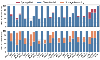
Figure 3: Percentage of fired neurons in VGG16 for CIFAR10. Each bar shows the average percentage of positive activations in VGG16’s layers for the specified attack.

In Figure 4, we show the energy increase per attacked layer for both StarGAN translation tasks. The graph shows that SpongeNet on StarGAN has the same behavior as SpongeNet on vision models. Indeed, most of the energy increase happens in the first few layers. Again, this is due to the first few layers containing the most activations and also still being able to change parameters by larger amounts without negatively affecting the performance of StarGAN.

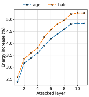
Figure 4: Energy increases of SpongeNet after every layer on StarGAN. SpongeNet attacks for both translation tasks were done with threshold SSIM = 0.05.

5.3 Ablation Study

For SpongeNet, we perform an ablation study on the accuracy drop thresholds of 0, 1, 2, and 5%. In Figures 5 and 6, we show the energy increase based on the number of attacked layers for different accuracy thresholds for VGG16 and ResNet18, respectively. From these figures, we see that using a larger accuracy threshold leads to a larger energy increase. However, this is a trade-off that the attacker needs to consider, as a decrease in accuracy could make the victim suspicious of the used model. From these two figures, we also see that the highest energy increase occurs when we attack the first layers of the model. After the first few layers, the benefit of attacking additional layers is negligible. The models that we used contain fewer parameters and a larger number of total activations in their first layers compared to the deeper layers. Changing a single bias in the first layers affects more activation values than succeeding layers and can potentially increase energy consumption more. This gives SpongeNet a double benefit, as targeting such layers makes the attack faster (fewer parameters) and more effective (more activations). We hypothesize that the negligible energy increase in the later layers is also partly due to the accuracy threshold being hit immediately after the attack has been performed on the first layer of the model, as can be seen in Figures 7 and 11.

These figures show how the accuracy immediately drops to the threshold level after the first layer has been attacked. This means that in succeeding layers, the attack can only alter biases that do not affect accuracy, resulting in fewer biases being increased and with smaller values. Thus, succeeding layers cause less energy increase. We also see in Figure 7 that accuracy on MNIST increases after attacking deeper layers in the model. By looking at the y-axis, this increase is negligible. However, we hypothesize that other parameters in the model are changing due to the bias increase, and as a result, the output layer’s activation value distribution is closer to the clean output layer’s distribution.

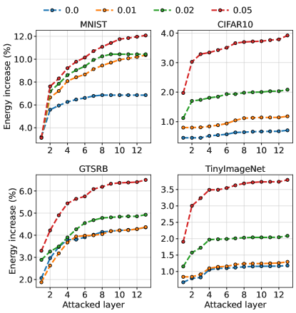
Figure 5: Evaluation of the SpongeNet threshold parameter on VGG16.

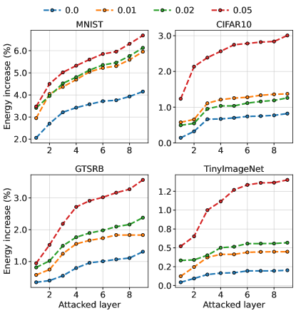
Figure 6: Evaluation of the SpongeNet threshold parameter on ResNet18. We display the mean energy ratios for several SpongeNet variations.

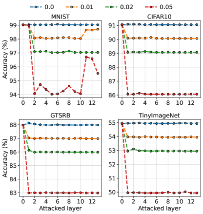
Figure 7: Accuracy of VGG16 during the SpongeNet attack for different thresholds.

5.4 Ablation For Stepsize on VGG16 and CIFAR10

Figure 8 shows the energy increase for the SpongeNet attack on VGG16 trained on CIFAR10. The attacker can get more energy increase at the cost of computation time by decreasing the step size parameter $\alpha$. SpongeNet keeps increasing the bias by $\alpha$ per step until $\alpha=2$, the accuracy drop exceeds the threshold, or the energy decreases after changing the bias. A smaller step size $\alpha$ means these three conditions are typically met after performing more steps than with a larger $\alpha$. Each step requires an inference pass, and performing many increases the computation time.

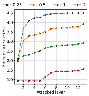
Figure 8: Energy increases for VGG16 trained on CIFAR10 after performing the SpongNet attack with different values for step size parameter $\alpha$.

5.5 Defenses

We now examine whether a defender can mitigate the sponge effects caused by Sponge Poisoning and SpongeNet. The results of the typical implementations of the defenses on the convolutional parameters are given in Table 2 and Table 4. The results for the adaptive defender defenses are given in Table 3, Table 5 and Table 6. For clipping, the defender only clips to a maximum positive value. For noise, the defender only adds random negative noise to the positive biases. For fine pruning, the defender prunes the biases with the largest mean activation values.

5.5.1 Parameter Perturbations

Table 2 contains the energy ratio increase before and after applying random noise to convolutional weights. The table shows that adding random noise to convolutional weights fails to mitigate the sponge effect on all models and datasets for both SpongeNet and Sponge Poisoning. We believe this failure can be attributed to the defenses being applied to the weight parameters of convolutional layers. Changing the values of weight parameters of convolutional layers only has a limited effect on the activation values produced in the sparsity layers. Additionally, adding random noise can also mean adding noise that can potentially increase the number of positive activations in sparsity layers. In contrast, Table 3 shows that targeting the sparsity layers during the defense and only adding negative noise reduces the increased energy consumption. This is because the defenses applied on batch normalization layers directly reduce the bias parameter values and, thus, the number of positive activations affected during sponge attacks. The same observations are made for the normal and adapted clipping defenses shown in Table 4 and Table 5.

Table 2: Resilience of SpongeNet and Sponge Poisoning against adding random noise to convolutional weights.

Network	Dataset	SpongeNet	SP
VGG16	MNIST	11.9 / 11.8	8.5 / 8.9
	CIFAR10	4.1 / 4.0	32.4 / 32.6
	GTSRB	6.7 / 6.5	25.8 / 25.8
	TIN	3.3 / 3.3	38.4 / 38.6
ResNet18	MNIST	6.5 / 6.7	6.0 / 6.4
	CIFAR10	2.9 / 3.0	22.5 / 22.6
	GTSRB	3.5 / 3.6	13.4 / 13.6
	TIN	1.4 / 1.4	25.0 / 24.8
StarGAN	Age	5.1 / 4.8	1.7 / 1.5
	Black hair	5.3 / 5.3	1.6 / 1.4

Table 3: Resilience of SpongeNet and Sponge Poisoning against adding random negative noise to batch normalization biases.

Network	Dataset	SpongeNet	SP
VGG16	MNIST	11.2 / 11.8	7.9 / 8.9
	CIFAR10	0.4 / 4.0	32.3 / 32.6
	GTSRB	3.9 / 6.5	25.4 / 25.8
	TIN	1.8 / 3.3	38.5 / 38.6
ResNet18	MNIST	4.6 / 6.7	5.7 / 6.4
	CIFAR10	0.8 / 3.0	22.6 / 22.6
	GTSRB	2.0 / 3.6	12.9 / 13.6
	TIN	0.7 / 1.4	24.6 / 24.8
StarGAN	Age	2.1 / 4.8	-1.2 / 1.5
	Black hair	2.4 / 5.3	- 1.1 / 1.4

Table 4: Resilience of SpongeNet and Sponge Poisoning against the clipping defense on convolutional weights.

Network	Dataset	SpongeNet	SP
VGG16	MNIST	12.9 / 11.8	10.4 / 8.9
	CIFAR10	4.2 / 4.0	32.9 / 32.6
	GTSRB	6.2 / 6.5	26.0 / 25.8
	TIN	3.2 / 3.3	38.7 / 38.6
ResNet18	MNIST	6.8 / 6.7	6.5 / 6.4
	CIFAR10	3.1 / 3.0	22.6 / 22.6
	GTSRB	3.7 / 3.6	14.1 / 13.6
	TIN	1.5 / 1.4	25.0 / 24.8
StarGAN	Age	4.6 / 4.8	1.5 / 1.5
	Black hair	5.2 / 5.3	1.7 / 1.4

Table 5: Resilience of SpongeNet and Sponge Poisoning against the clipping defense on batch normalization biases.

Network	Dataset	SpongeNet	SP
VGG16	MNIST	10.7 / 11.8	0.1 / 8.9
	CIFAR10	1.5 / 4.0	32.3 / 32.6
	GTSRB	6.1 / 6.5	25.9 / 25.8
	TIN	3.2 / 3.3	38.5 / 38.6
ResNet18	MNIST	6.1 / 6.7	4.1 / 6.4
	CIFAR10	- 0.1 / 3.0	22.7 / 22.6
	GTSRB	- 1.3 / 3.6	13.0 / 13.6
	TIN	1.0 / 1.4	24.9 / 24.8
StarGAN	Age	-2.2 / 4.8	-1.2 / 1.5
	Black hair	-1.9 / 5.3	-0.9 / 1.4

5.5.2 Fine-pruning

Table 6 contains the energy ratio before and after fine-pruning and the accuracy/SSIM after applying the adapted defense. The table shows that the adapted fine-pruning defense can partly mitigate the effects of SpongeNet on vision models without affecting accuracy. Sponge-poisoned vision models are more resilient against the adapted defense. We hypothesize that Sponge Poisoning is better at maintaining accuracy than SpongeNet because, during Sponge Poisoning, the model is also trained to perform well on the relevant task with the classification loss. All of the model’s parameters are adjusted not only the sparsity layers. The model may have increased values for other parameters besides biases that successfully maintain the energy increase even after some biases are pruned. Meanwhile, SpongeNet is dependent on the increased values only for biases.

However, for GAN models, SpongeNet is more resilient against the adapted fine-pruning defense. The pre-defense SSIM for SpongeNet is reduced by a larger value than the SSIM for Sponge Poisoning, up to 0.15 compared to 0.03. Even though fine-pruning can reverse the increased energy consumption, it reduces the SSIM of images generated by a large amount. This can be seen in Figure 9. The figure contains images generated by SpongeNet StarGAN for 0.8 SSIM. Sponge-poisoned StarGAN shows similar results at 0.8 SSIM. The images show how an SSIM at and below 0.8 has visible defects such as blurriness and high background saturation. A defender might be able to mitigate the sponge effect from SpongeNet and Sponge Poisoning with the adapted defenses, but the SSIM will be reduced to such an extent that the images become visibly affected and of poor quality. Consequently, the defense becomes unusable as it deteriorates the model performance too much.

Table 6: Resilience of SpongeNet and Sponge Poisoning against fine-pruning. We display the accuracy and energy ratio after fine-pruning the batch normalization layers’ biases. The Acc. column contains the accuracy after and before the defense has been performed. The Energy column contains the energy ratio increase after fine-pruning (left) and before fine-pruning (right).

Network	Dataset	SpongeNet		SP
		Acc. (%)	Energy (%)	Acc. (%)	Energy (%)
VGG16	MNIST	98 / 94	11.9 / 11.8	98 / 97	7.8 / 8.9
	CIFAR10	90 / 86	1.9 / 4.0	75 / 89	31.6 / 32.6
	GTSRB	85 / 83	4.9 / 6.5	51 / 74	25.8 / 25.8
	TIN	55 / 50	2.9 / 3.3	52 / 44	37.8 / 38.6
ResNet18	MNIST	98 / 94	4.5 / 6.7	99 / 98	5.7 / 6.4
	CIFAR10	91 / 87	0.8 / 3.0	91 / 91	22.7 / 22.6
	GTSRB	93 / 88	3.8 / 3.6	92 / 92	12.5 / 13.6
	TIN	56 / 52	1.3 / 1.4	54 / 54	25.3 / 24.8
StarGAN	Age	0.84 / 0.95	1.3 / 4.8	0.83 / 0.84	1.0 / 1.5
	Black hair	0.80 / 0.95	1.2 / 5.3	0.81 / 0.84	0.9 / 1.4

(a) Aging translation

(b) Black hair translation

Figure 9: Degradation of generation performance. Translation images produced with SSIM $\leq$ 0.80 to the regular GAN-generated images. At 0.80 SSIM and below, the generated images have visible issues such as blurriness and background saturation.

5.6 User Study

Methodology. We designed a questionnaire to evaluate whether the images created with SpongeNet or Sponge Poisoning are more stealthy. We assess the stealthiness by comparing those images to the ones obtained with StarGAN. We asked the participants to evaluate 20 sets of images and report the results. Each image set consists of three images: in the first row, the original image from StarGAN, and in the second row, two images (in random order to avoid bias in the answers) from Sponge Poisoning and SpongeNet. We did not apply any particular restriction to the participants during the filling of the questionnaire. In particular, there were no time restrictions to complete the task.

We conducted two rounds of the experiments. In the first round, we provided the participants only basic information that the goal was to observe images and report which one from the second row was more similar to the one in the first row. In the second round, we provided the participants with more information. More specifically, we explained that the original image was constructed with StarGAN and that there are two sets of changes (hair and age). Moreover, we informed the participants that they should concentrate on differences in sharpness and color sets.

First round. A total of 47 (32 male, age 36.09$\pm 10.34$, 14 female, age 34.86$\pm 4.04$, and one non-binary age 29) participants completed the experiment. There were no requirements on a person’s background, nor did the participants receive any info beyond the task to differentiate between images. 87.02% of the answers indicated that SpongeNet images are more similar to the StarGAN images than Sponge Poisoning images. Thus, even participants who are not informed about the details of the experiment recognize, in the majority of the cases, SpongeNet images as closer to the real images.

Second round. A total of 16 (12 male, age 23.27 $\pm 1.56$ and 4 female, age 23.5 $\pm 1.29$) participants completed the experiment. The participants in this phase have computer science backgrounds and have knowledge about the security of machine learning and sponge attacks. Moreover, the participants were informed about the details of the experiment (two different attacks and two different transformations). 87.19% of the answers indicated that SpongeNet images are more similar to the StarGAN images than Sponge Poisoning images.

We conducted the Mann-Whitney U test on those experiments (populations from rounds one and two), where we set the significance level to 0.01, and 2-tailed hypothesis, and the result shows there is no statistically significant difference. As such, we can confirm that SpongeNet is more stealthy than Sponge Poisoning, and the knowledge about the attacks does not make any difference.

5.7 Discussion

We believe SpongeNet is a practical and important threat we should consider. It results in a smaller energy increase than Sponge Poisoning[9] for vision models but cannot be easily spotted by a defender through an analysis of the activations of the model. Moreover, SpongeNet is more effective than Sponge Poisoning in increasing StarGAN’s energy consumption. Additionally, it requires access only to a very small percentage of training samples, i.e., one batch of samples may be enough, and the model’s weights. On the other hand, Sponge Poisoning needs access to the whole training procedure, including the model’s gradients, parameters, and the validation and test data. Moreover, SpongeNet is more flexible than Sponge Poisoning as it can alter only individual layers or only individual parameters within specific layers. Sponge poisoning alters the entire model. SpongeNet also allows the attacker to set an energy cap to avoid detection, which is not possible with Sponge Poisoning.

6 Related Work

The first work on sponge attacks was introduced by Shumailov et al. [7] with their sponge examples. They created sponge examples with genetic algorithms to attack transformer language translation networks. For vision models, they used genetic algorithms(GA) and LBFGS. According to their results, Sponge LBFGS samples perform better than GA on vision models and can achieve around a maximum of 3% energy increase in the model compared to normal samples. Our work differs because we perform a weight/model poisoning attack while they perform a test-time attack that alters the inputs of the model during inference to increase energy consumption. Additionally, we use the $\ell_{0}$ norm instead of $\ell_{2}$ norm, which focuses on the number of activations, to increase the energy consumption of targeted models. Following this work, Cina et al. introduced the Sponge Poisoning [9]. They argued that sponge examples can easily be detected if the queries are not sufficiently different and are computationally expensive. Moreover, they showed that the $\ell_{2}$ distance used for sponge examples [7] performs worse for vision models than $\ell_{0}$. This was experimentally shown with their code poisoning attack. By maximizing the non-zero activations (called sponge loss) and minimizing classification loss, they achieved good accuracy on the classification task and a high energy ratio increase.

We also use several hyperparameters defined in this paper: $\sigma$ represents the preciseness of the $L_{0}$ approximation, $\lambda$ represents the weight given to the sponge loss compared to the classification loss, and finally, $\delta$ or just $p$ is the percentage of data for which the altered objective function is applied. (An extra limitation from this is the extra inference pass required for the sponged sampled during training, = more cost). Sponge poisoning in Cina et al. [9] is only performed on vision models, but we perform Sponge Poisoning on a GAN, which required us to extend the ASIC simulator to work with Instance normalization layers and the Tanh activation function. Sponge poisoning has also been applied to mobile phones. In particular, Paul et al. [10] found that Sponge Poisoning could increase the inference time on average by 13% and deplete the phone battery 15% faster on low-end devices. On the other hand, Wang et al. [28] showed that mobile devices that contain more advanced accelerators for deep learning computations may be more vulnerable to Sponge Poisoning.

Shapira et al.[8] were the first to consider sponging an object detection pipeline and focused on increasing the latency of various YOLO models. They achieve increased latency by creating a universal adversarial perturbation (UAP) on the input images with projected gradient descent with the L2 norm. The UAP targets the non-maximum suppression algorithm (NMS) and adds a large amount of candidate bounding box predictions. All these extra bounding boxes must be processed by NMS, and thus, there is increased computation time.

Finally, Hong et al.[35] introduced their weight poisoning attack and showed that an attacker could directly alter the values of weights in convolutional layers without significantly affecting the accuracy of a model. They used this to backdoor attack models. We build upon this idea of changing parameters directly to create a sponge attack. We change the biases of batch normalization layers instead of convolutional weights to increase the number of activations and, in turn, increase the energy consumption.

7 Conclusions and Future Work

This work proposes a novel sponge attack on deep neural networks. The SpongeNet attack changes the parameters of the pre-trained model. By doing so, we enable our attack to be powerful (increasing energy consumption) and stealthy (making the detection more difficult). We conduct our experiments on vision and GAN models and five datasets and showcase the potential of our approach.

For future work, there are several interesting directions to follow. First, since there is only sparse work on sponge attacks, more investigations about potential attacks and defenses are needed. Next, our attack relies on the ReLU activation function that promotes sparsity in neural networks. However, there are other (granted, much less used) activation functions that could potentially bring even more sparsity [49, 50]. Investigating the attack performance for those settings would be then interesting. Lastly, in this work, we used an ASIC accelerator simulator as provided by [7]. Other methods to estimate the energy consumption of DNNs are possible [51] and would constitute an interesting extension of this work.

Appendix A ReLU vs. LeakyReLU

Table 7 contains the percentage of energy ratio increase and energy ratio of SpongeNet on VGG16 with ReLU as activation layers versus LeakyReLU as activation layers. The energy ratio is the ratio between the average case and the worst case, as described in Section 2. As can be seen, the ratio for the clean model is already at 1.0 before any attack has been performed, meaning there is no sparsity. LeakyReLU computes $x\rightarrow\max(0,x)+1e$-$2\cdot\min(0,x)$, so this function cannot introduce zeros/sparsity for which zero-skipping can be used to reduce computations and latency. Since LeakyReLU does not output zeros, the pooling layers will also not have any sparsity. This can be seen in Figure 10.

Table 7: Energy increases if we swap out ReLU for LeakyRELU. Ratio = 1.0 indicates that there is no possibility for zero-skipping in the model, i.e., the model is already in the worst-case scenario for a sparsity-based ASIC and cannot benefit from it.

Network	Dataset	ReLU		LeakyReLU
		Increase (%)	Ratio	Increase (%)	Ratio
VGG16	MNIST	11.8	0.74	0.0	1.0
	CIFAR10	4.0	0.68	0.0	1.0
	GTSRB	6.5	0.66	0.0	1.0
	TIN	3.3	0.67	0.0	1.0

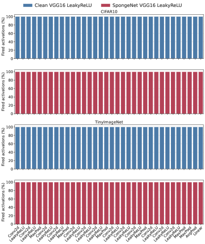
Figure 10: Fired percentages of LeakyReLU VGG16 networks for CIFAR10 and TinyImageNet datasets.

Appendix B SpongeNet Threshold Ablation Study

We display the accuracy for each attack layer during the ablation study on ResNet18 in Figure 11. The given accuracy is calculated on the entire validation set. The accuracy immediately drops to the threshold value after the first layer is attacked, decreasing the benefit of attacking more layers.

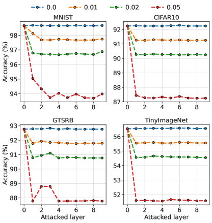
Figure 11: Accuracy for ResNet18 during the SpongeNet attack for different thresholds.

Appendix C Fired Percentage Graphs SpongeNet

In Figure 12, we show the average fired percentage on the validation set per layer for the SpongeNet attack on VGG16. In Figure 13, we show the average fired percentage on the validation set per layer. Graphs are for SpongeNet with threshold = 0.05. In Figure 12, it can be seen that for all datasets except MNIST, SpongeNet on VGG16 does not increase the fired percentage in every layer and typically does so for less than 10%. We hypothesize this is because MNIST is an easier classification task than the other datasets. Thus, even if many changes are made to the model’s parameters, the accuracy can remain high and above the SpongeNet threshold. This same behavior can be observed for SpongeNet on ResNet18 in Figure 6, where for MNIST, the attack can increase the fired percentage of some layers of the model by 10% more than for other datasets. Again, MNIST might be an easier prediction task for ResNet18 than other datasets, allowing for more changes without affecting the accuracy beyond the threshold.

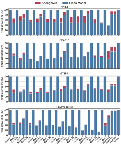
Figure 12: We display the differences in the average percentage of positive activations in all layers for a clean VGG16 model and VGG16 after the SpongeNet attack. The average is calculated over all images in the validation set.

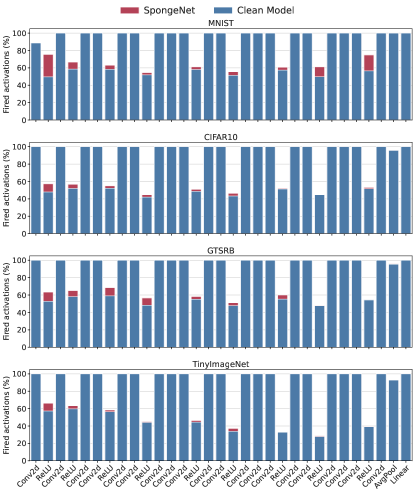
Figure 13: We display the differences in the average percentage of positive activations in all layers for a clean ResNet18 model and ResNet18 after the SpongeNet attack. The average is calculated over all images in the validation set.

Appendix D Fired Percentage Graphs Sponge Poisoning

In Figure 14, we show the average fired percentage on the validation set per layer for VGG16 and for ResNet18 in Figure 15. Graphs are for Sponge Poisoning with $\lambda=2.5$, $p=0.05$ and $\sigma=1e-04$. In the figures, we see that sponge causes a fired percentage increase in all layers of VGG16 and ResNet18 for all datasets, typically by 10% or more. We hypothesize that this is because Sponge Poisoning benefits from including the classification loss during training and can maintain the performance of the model by adjusting other parameters in the model to compensate for the increased bias values in the batch normalization layers.

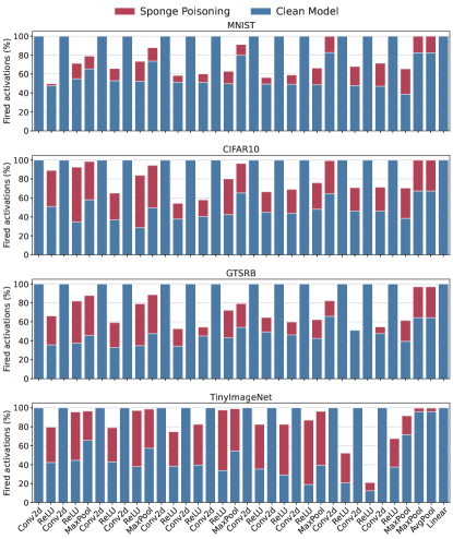
Figure 14: We display the differences in the average percentage of positive activations in all layers for a clean VGG16 model and a Sponge Poisoned VGG16 model. The average is calculated over all images in the validation set.

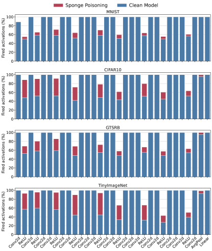
Figure 15: The differences in the average percentage of positive activations in all layers for a clean ResNet18 model and a Sponge Poisoned ResNet18 model. The average is calculated over all images in the validation set.

References

- [1] R. S. S. Kumar, D. O. Brien, K. Albert, S. Viljöen, and J. Snover, “Failure modes in machine learning systems,” arXiv preprint arXiv:1911.11034, 2019.
- [2] C. Szegedy, W. Zaremba, I. Sutskever, J. Bruna, D. Erhan, I. Goodfellow, and R. Fergus, “Intriguing properties of neural networks,” arXiv preprint arXiv:1312.6199, 2013.
- [3] T. Gu, B. Dolan-Gavitt, and S. Garg, “Badnets: Identifying vulnerabilities in the machine learning model supply chain,” arXiv preprint arXiv:1708.06733, 2017.
- [4] M. Jagielski, N. Carlini, D. Berthelot, A. Kurakin, and N. Papernot, “High accuracy and high fidelity extraction of neural networks,” in 29th USENIX security symposium (USENIX Security 20), pp. 1345–1362, 2020.
- [5] R. Shokri, M. Stronati, C. Song, and V. Shmatikov, “Membership inference attacks against machine learning models,” in 2017 IEEE symposium on security and privacy (SP), pp. 3–18, IEEE, 2017.
- [6] M. Fredrikson, S. Jha, and T. Ristenpart, “Model inversion attacks that exploit confidence information and basic countermeasures,” in Proceedings of the 22nd ACM SIGSAC conference on computer and communications security, pp. 1322–1333, 2015.
- [7] I. Shumailov, Y. Zhao, D. Bates, N. Papernot, R. Mullins, and R. Anderson, “Sponge examples: Energy-latency attacks on neural networks,” in 2021 IEEE European Symposium on Security and Privacy (EuroS&P), pp. 212–231, 2021.
- [8] A. Shapira, A. Zolfi, L. Demetrio, B. Biggio, and A. Shabtai, “Phantom sponges: Exploiting non-maximum suppression to attack deep object detectors,” in 2023 IEEE/CVF Winter Conference on Applications of Computer Vision (WACV), pp. 4560–4569, 2023.
- [9] A. E. Cinà, A. Demontis, B. Biggio, F. Roli, and M. Pelillo, “Energy-latency attacks via sponge poisoning,” ArXiv, vol. abs/2203.08147, 2022.
- [10] S. Paul and N. Kourtellis, “Sponge ml model attacks of mobile apps,” in Proceedings of the 24th International Workshop on Mobile Computing Systems and Applications, HotMobile ’23, (New York, NY, USA), p. 139, Association for Computing Machinery, 2023.
- [11] D. Patterson, J. M. Gilbert, M. Gruteser, E. Robles, K. Sekar, Y. Wei, and T. Zhu, “Energy and emissions of machine learning on smartphones vs. the cloud,” Commun. ACM, vol. 67, p. 86–97, jan 2024.
- [12] S. Samsi, D. Zhao, J. McDonald, B. Li, A. Michaleas, M. Jones, W. Bergeron, J. Kepner, D. Tiwari, and V. Gadepally, “From words to watts: Benchmarking the energy costs of large language model inference,” 2023.
- [13] D. Patterson, J. Gonzalez, Q. Le, C. Liang, L.-M. Munguia, D. Rothchild, D. So, M. Texier, and J. Dean, “Carbon emissions and large neural network training,” 2021.
- [14] M. R. Azghadi, C. Lammie, J. K. Eshraghian, M. Payvand, E. Donati, B. Linares-Barranco, and G. Indiveri, “Hardware implementation of deep network accelerators towards healthcare and biomedical applications,” IEEE Transactions on Biomedical Circuits and Systems, vol. 14, no. 6, pp. 1138–1159, 2020.
- [15] R. Machupalli, M. Hossain, and M. Mandal, “Review of asic accelerators for deep neural network,” Microprocessors and Microsystems, vol. 89, p. 104441, 2022.
- [16] K. Liu, B. Dolan-Gavitt, and S. Garg, “Fine-pruning: Defending against backdooring attacks on deep neural networks,” in Research in Attacks, Intrusions, and Defenses, p. 273–294, Springer International Publishing, 2018.
- [17] D. Kim, J. Ahn, and S. Yoo, “A novel zero weight/activation-aware hardware architecture of convolutional neural network,” in Proceedings of the Conference on Design, Automation & Test in Europe, DATE ’17, (Leuven, BEL), p. 1466–1471, European Design and Automation Association, 2017.
- [18] Y. Zhang, H. Jiang, X. Li, H. Wang, D. Dong, and Y. Cao, “An efficient sparse cnns accelerator on fpga,” in 2022 IEEE International Conference on Cluster Computing (CLUSTER), pp. 504–505, 2022.
- [19] A. Parashar, M. Rhu, A. Mukkara, A. Puglielli, R. Venkatesan, B. Khailany, J. Emer, S. W. Keckler, and W. J. Dally, “Scnn: An accelerator for compressed-sparse convolutional neural networks,” in 2017 ACM/IEEE 44th Annual International Symposium on Computer Architecture (ISCA), pp. 27–40, 2017.
- [20] Y.-H. Chen, T. Krishna, J. S. Emer, and V. Sze, “Eyeriss: An energy-efficient reconfigurable accelerator for deep convolutional neural networks,” IEEE Journal of Solid-State Circuits, vol. 52, no. 1, pp. 127–138, 2017.
- [21] M. Nikolić, M. Mahmoud, and A. Moshovos, “Characterizing sources of ineffectual computations in deep learning networks,” in 2018 IEEE International Symposium on Workload Characterization (IISWC), pp. 86–87, 2018.
- [22] X. Glorot, A. Bordes, and Y. Bengio, “Deep sparse rectifier neural networks,” in Proceedings of the Fourteenth International Conference on Artificial Intelligence and Statistics (G. Gordon, D. Dunson, and M. Dudík, eds.), vol. 15 of Proceedings of Machine Learning Research, (Fort Lauderdale, FL, USA), pp. 315–323, PMLR, 11–13 Apr 2011.
- [23] A. Krizhevsky, I. Sutskever, and G. E. Hinton, “Imagenet classification with deep convolutional neural networks,” in Proceedings of the 25th International Conference on Neural Information Processing Systems - Volume 1, NIPS’12, (Red Hook, NY, USA), p. 1097–1105, Curran Associates Inc., 2012.
- [24] J. Albericio, P. Judd, T. Hetherington, T. Aamodt, N. E. Jerger, and A. Moshovos, “Cnvlutin: Ineffectual-neuron-free deep neural network computing,” in 2016 ACM/IEEE 43rd Annual International Symposium on Computer Architecture (ISCA), pp. 1–13, 2016.
- [25] S. Han, X. Liu, H. Mao, J. Pu, A. Pedram, M. A. Horowitz, and W. J. Dally, “Eie: Efficient inference engine on compressed deep neural network,” 2016.
- [26] A. Parashar, M. Rhu, A. Mukkara, A. Puglielli, R. Venkatesan, B. Khailany, J. Emer, S. W. Keckler, and W. J. Dally, “Scnn: An accelerator for compressed-sparse convolutional neural networks,” 2017.
- [27] I. Mirzadeh, K. Alizadeh, S. Mehta, C. C. D. Mundo, O. Tuzel, G. Samei, M. Rastegari, and M. Farajtabar, “Relu strikes back: Exploiting activation sparsity in large language models,” 2023.
- [28] Z. Wang, S. Huang, Y. Huang, and H. Cui, “Energy-latency attacks to on-device neural networks via sponge poisoning,” in Proceedings of the 2023 Secure and Trustworthy Deep Learning Systems Workshop, SecTL ’23, (New York, NY, USA), Association for Computing Machinery, 2023.
- [29] B. K. Natarajan, “Sparse approximate solutions to linear systems,” SIAM Journal on Computing, vol. 24, no. 2, pp. 227–234, 1995.
- [30] M. R. Osborne, B. Presnell, and B. A. Turlach, “On the lasso and its dual,” Journal of Computational and Graphical Statistics, vol. 9, pp. 319 – 337, 2000.
- [31] P. Isola, J.-Y. Zhu, T. Zhou, and A. A. Efros, “Image-to-image translation with conditional adversarial networks,” in 2017 IEEE Conference on Computer Vision and Pattern Recognition (CVPR), pp. 5967–5976, 2017.
- [32] J.-Y. Zhu, T. Park, P. Isola, and A. A. Efros, “Unpaired image-to-image translation using cycle-consistent adversarial networks,” in 2017 IEEE International Conference on Computer Vision (ICCV), pp. 2242–2251, 2017.
- [33] Y. Choi, M. Choi, M. Kim, J.-W. Ha, S. Kim, and J. Choo, “Stargan: Unified generative adversarial networks for multi-domain image-to-image translation,” in 2018 IEEE/CVF Conference on Computer Vision and Pattern Recognition, pp. 8789–8797, 2018.
- [34] Z. Wang, A. C. Bovik, H. R. Sheikh, and E. P. Simoncelli, “Image quality assessment: from error visibility to structural similarity,” IEEE transactions on image processing, vol. 13, no. 4, pp. 600–612, 2004.
- [35] S. Hong, N. Carlini, and A. Kurakin, “Handcrafted backdoors in deep neural networks,” in Advances in Neural Information Processing Systems (A. H. Oh, A. Agarwal, D. Belgrave, and K. Cho, eds.), 2022.
- [36] J. Frankle and M. Carbin, “The lottery ticket hypothesis: Finding sparse, trainable neural networks,” 2019.
- [37] K. He, X. Zhang, S. Ren, and J. Sun, “Deep residual learning for image recognition,” in Proceedings of the IEEE conference on computer vision and pattern recognition, pp. 770–778, 2016.
- [38] K. Simonyan and A. Zisserman, “Very deep convolutional networks for large-scale image recognition,” arXiv preprint arXiv:1409.1556, 2014.
- [39] Y. LeCun, C. Cortes, and C. Burges, “The mnist handwritten digit database,” ATT Labs [Online]. Available: http://yann.lecun.com/exdb/mnist, vol. 2, 2010.
- [40] A. Krizhevsky, G. Hinton, et al., “Learning multiple layers of features from tiny images,” 2009.
- [41] S. Houben, J. Stallkamp, J. Salmen, M. Schlipsing, and C. Igel, “Detection of traffic signs in real-world images: The german traffic sign detection benchmark,” The 2013 International Joint Conference on Neural Networks (IJCNN), pp. 1–8, 2013.
- [42] Y. Le and X. Yang, “Tiny imagenet visual recognition challenge,” CS 231N, vol. 7, no. 7, p. 3, 2015.
- [43] Z. Liu, P. Luo, X. Wang, and X. Tang, “Deep learning face attributes in the wild,” in Proceedings of International Conference on Computer Vision (ICCV), December 2015.
- [44] M. Zhao, F. Bao, C. LI, and J. Zhu, “Egsde: Unpaired image-to-image translation via energy-guided stochastic differential equations,” in Advances in Neural Information Processing Systems (S. Koyejo, S. Mohamed, A. Agarwal, D. Belgrave, K. Cho, and A. Oh, eds.), vol. 35, pp. 3609–3623, Curran Associates, Inc., 2022.
- [45] D. Torbunov, Y. Huang, H. Yu, J. Huang, S. Yoo, M. Lin, B. Viren, and Y. Ren, “Uvcgan: Unet vision transformer cycle-consistent gan for unpaired image-to-image translation,” in 2023 IEEE/CVF Winter Conference on Applications of Computer Vision (WACV), pp. 702–712, 2023.
- [46] D. Torbunov, Y. Huang, H.-H. Tseng, H. Yu, J. Huang, S. Yoo, M. Lin, B. Viren, and Y. Ren, “Uvcgan v2: An improved cycle-consistent gan for unpaired image-to-image translation,” 2023.
- [47] Y. Choi, Y. Uh, J. Yoo, and J.-W. Ha, “Stargan v2: Diverse image synthesis for multiple domains,” in Proceedings of the IEEE Conference on Computer Vision and Pattern Recognition, 2020.
- [48] Z. Wang, A. Bovik, H. Sheikh, and E. Simoncelli, “Image quality assessment: from error visibility to structural similarity,” IEEE Transactions on Image Processing, vol. 13, no. 4, pp. 600–612, 2004.
- [49] M. Kurtz, J. Kopinsky, R. Gelashvili, A. Matveev, J. Carr, M. Goin, W. Leiserson, S. Moore, N. Shavit, and D. Alistarh, “Inducing and exploiting activation sparsity for fast inference on deep neural networks,” in Proceedings of the 37th International Conference on Machine Learning (H. D. III and A. Singh, eds.), vol. 119 of Proceedings of Machine Learning Research, pp. 5533–5543, PMLR, 13–18 Jul 2020.
- [50] P. Bizopoulos and D. Koutsouris, “Sparsely activated networks,” IEEE Transactions on Neural Networks and Learning Systems, vol. 32, p. 1304–1313, Mar. 2021.
- [51] T.-J. Yang, Y.-H. Chen, J. Emer, and V. Sze, “A method to estimate the energy consumption of deep neural networks,” in 2017 51st Asilomar Conference on Signals, Systems, and Computers, pp. 1916–1920, 2017.