Photon Number-Resolving Quantum Reservoir Computing

Abstract

Neuromorphic processors improve the efficiency of machine learning algorithms through the implementation of physical artificial neurons to perform computations. However, whilst efficient classical neuromorphic processors have been demonstrated in various forms, practical quantum neuromorphic platforms are still in the early stages of development. Here we propose a fixed optical network for photonic quantum reservoir computing that is enabled by photon number-resolved detection of the output states. This significantly reduces the required complexity of the input quantum states while still accessing a high-dimensional Hilbert space. The approach is implementable with currently available technology and lowers the barrier to entry to quantum machine learning.

Introduction. Quantum machine learning (QML) is a broad field in which the physical features of quantum systems are leveraged to process data [1]. In addition to promising speedups for classical tasks, QML systems are able to directly process quantum data leading to improvements in existing methods of extracting and manipulating quantum information [2, 3]. Quantum neural networks (QNNs) are a subclass of QML in which the structure of artificial neural networks (ANNs) is composed of linked quantum states which, together with their interactions, may be parametrized and trained. Generally, these algorithms are implemented on quantum computers, the most promising of which use either superconducting qubits or squeezed states of light as their substrate. Although these devices show great promise to scale thanks to years of hard efforts [4, 5, 6, 7, 8, 9], the technology is out of reach for most laboratories and may indeed be overkill for many routine data processing tasks. This opens a door for neuromorphic hardware that can be specialized to various analysis tasks on classical or quantum data with minimal experimental overhead. Among the different hardware implementations of QNNs, linear photonic networks (LPNs) are of particular interest for reasons including: room-temperature operation, low power consumption, convenience of networking devices and scalability [10]. In addition, LPNs have a rich theoretical framework in place and have already been used to demonstrate forms of quantum computation [11, 12, 13, 14, 4, 15, 5, 16]. These results are promising in the context of a search for more efficient neuromorphic systems. Indeed, all approaches that require training of a large number of degrees of freedom come at significant computational and environmental costs, which are major motivations to develop optical ANNs [17].

Reservoir computing (RC) is particular sub-class of ANNs that have attracted attention as a viable and efficient neuromorphic platform. Characterized by its unique strategy of combining the collective hidden layers of an ANN into a single, random, high-dimensional layer with fixed dynamics, RC significantly mitigates the computational load typically associated with extensive ANN training. This is achieved by performing training solely at the readout stage. Implemented in LPNs, RC leverages the intrinsic complexity and high-dimensional state space generated by the platform. Coupled with the innate parallel processing strength and growth potential of LPNs, RC presents a compelling model for the future of large-scale and high-speed computing.

Here, we present the concept of photon number-resolving quantum reservoir computing (Photon-QuaRC). This is a quantum reservoir computer (QRC) based on a linear photonic network in which information is encoded and manipulated in the polarisation states of light. We improve computational power without increasing network complexity by applying photon number-resolved detection at the output. This is made possible through the combinatorial scaling of the output Hilbert space with the number of input photons. Furthermore, we show that we can retain the advantage gained through quantum multiphoton interference inside the network without having to prepare large photon-number Fock states. The reservoir architecture allows implementation in a wide range of simple physical systems such as multimode fibers or scattering materials [18, 19]. It also avoids the need to optimize the network and reduces all training energy costs to a matrix inversion. Due to these features, we present our method as a practical path towards versatile, scalable quantum machine learning.

Polarising linear optical networks as quantum reservoirs. Various forms of reservoir computers (RCs) have been studied extensively as they provide a framework for neural networks that can be naturally mapped to the dynamics of physical systems [20] including squeezed light in a circulating nonlinear cavity [21]. Several systems have been based on random optical media [19, 21] - we show that these can indeed be extended to QRCs based on a general BosonSampling scheme. Figure 1(a) shows the schematic layout of Photon-QuaRC: $N$ photons are fed into the physical system which is composed of two sequential $M$-port LPNs: the encoding layer, $E(x)$ which operates only on the polarisation degree of freedom of the input state and the reservoir, $R$ which couples both spatial and polarisation modes. Encoding follows trajectories on a Poincarè sphere, schematically indicated in the figure. The output then consists of Fock state distributions $F(x)$ that we can then use to solve the task of interpolating generic functions, $f(x)$. This is achieved with a training phase, outlined in Fig. 1(b) where the weights $W$ are learned and then used in the inference phase, Fig. 1(c) to perform machine learning tasks, e.g. function interpolation. We now provide more details for each of these steps.

Quantum reservoir computer output. For input data $x$ the output of the QRC is

$$\langle\vec{F}(x)\rangle=\langle\vec{n}^{in}\mathcal{E^{{\dagger}}}(x)\mathcal{R^{{\dagger}}}|\vec{F}|\mathcal{RE}(x)\vec{n}^{in}\rangle,$$ (1)

where $\mathcal{R}$ and $\mathcal{E}(x)$ are the unitary Fock space scattering matrices corresponding to the reservoir and encoding transformations, respectively. These may be built from the mode-coupling matrices of the corresponding LPNs as shown in Ref. [22]. $\langle\vec{F}(x)\rangle$ denotes the probability distribution over the $d=\binom{N+M-1}{N}$ measurement outcomes at the reservoir output, and $|\vec{n}^{in}\rangle$ is the input Fock state, prior to the encoding. The scaling of $d$ with $N$ is a key feature of the BosonSampling approach as it allows us to expand the feature space combinatorially faster than the physical network complexity.

The target function is approximated from the reservoir output by a matrix multiplication

$$\vec{f}(x)=W\langle\vec{F}(x)\rangle,$$ (2)

where $W$ is the weight matrix learned from linear regression on labelled data.

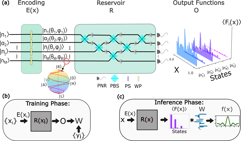
Figure 1: Photon-QuaRC schematic overview. (a) Horizontally polarised Fock and coherent states in $M$ different spatial modes are directed into an encoding block $E(x)$ that encodes the input data, $x$, in a multimode polarisation state. The polarisation at each port is parametrized on the Poincaré Sphere by $\theta_{m}$ and $\phi_{m}$, which are the azimuth and zenith angles, respectively. This state is fed into a random, fixed linear optical network built from polarising beamsplitters (PBS), waveplates (WP) and phase shifters (PS). Output states are subject to polarisation-independent measurement by photon number-resolving (PNR) detectors. Approximation of the Fock state distribution $\langle\vec{\hat{F}}(x)\rangle$ by repeated sampling constitutes the device output, Eq. (1). (b) During the training stage, labelled data $\{x_{i}\}$ are encoded, and the reservoir outputs are saved in an array $O$. The elements of this array are then fit to labels $\{y_{i}\}$ to learn weights, $W$. (c) In the inference phase the target function $\vec{f}(x)$ on input data is evaluated by multiplying $\langle\vec{\hat{F}}(x)\rangle$ by $W$, Eq. (2).

Prior BosonSampling-inspired approaches to QML use networks made of trainable blocks that are tuned to produce a desired target function [23]. However, a key feature of the Photon-QuaRC architecture is that the target function is computed without having to optimize over the network parameters.

Fourier space feature learning. Previous work has shown that the output of any quantum neural network can be expressed as a partial Fourier series of the data [23, 24, 25]. This output $g(x)$ can be written as

$$g(x)=\sum_{\omega\in\Omega_{n}}c_{\omega}e^{i\omega x},$$ (3)

where $\Omega_{n}$ is the set of all unique frequencies that the network can generate. Frequencies $\omega\in\Omega_{n}$ are determined by the encoding scheme and the number of input photons, while the coefficients $c_{\omega}$ are fixed by the network structure. The properties of $\Omega_{n}$ (size, center and maximum frequency) determine the class of functions that the network can approximate, a.k.a. expressivity. However, while $\Omega_{n}$ contains information about the ability of a given design to specialize to a task, it does not provide a characterization of the robustness under operation, as we discuss below.

A primary challenge in scaling the feature space in QML using optical systems is generating large-photon-number Fock states, which can be prohibitive in practice. While these high-photon-number states offer optimal performance within certain constraints, it prompts us to consider whether comparable results can be achieved with fewer quantum resources. For example, prior work has shown that by leveraging the interference between a single-photon Fock state and a coherent state, one can create quantum mechanical states with arbitrary photon numbers [26, 27]. This approach also requires photon number-resolving detection and post-selection, so as to distill quantum interference of the desired order from the output.

We adopt this concept and therefore start from a general state that combines coherent and Fock components in a unified form,

$$|\psi_{\vec{\alpha},\vec{n}}\rangle=\prod_{m=1}^{M}e^{\alpha_{m}a_{m}^{{\dagger}}-\alpha_{m}^{*}a_{m}}\frac{(a_{m}^{{\dagger}})^{n_{m}}}{\sqrt{n_{m}!}}|0\rangle,$$ (4)

where $\alpha_{m}$ and $n_{m}$ are the coherent state amplitude and number of added photons in mode $m$ respectively. If the $\alpha_{m}$ or $n_{m}$ are set to zero, Eq. (4) simplifies to the standard form of a Fock state or a coherent state, respectively. Any state with non-zero $n_{m}$ and $\alpha_{m}$ is referred to as a hybrid state. In what follows we will notate a Hybrid state as $|\psi_{\vec{\alpha},\vec{n}}\rangle=|\alpha_{1}+n_{1},...,\alpha_{m}+n_{m}\rangle$ (see SM for more details).

Model of polarising network. We construct the network adapting the method proposed by Reck et al. [28] with some key modifications: we replace each spatial mode with a pair of corresponding polarisation modes and the constituent optical elements are polarising beamsplitters, arbitrary birefringent waveplates and phase shifters. The full network then couples 2M modes, and the primitive elements operate on 4x4 subspaces (see the SM for details).

The input to the QRC is a fixed state which is encoded with the data and scattered into a superposition of Fock states at the output. To describe the action of the encoding layer at each input port we apply the ladder operator replacement rule

$$a_{m}^{{\dagger}}\rightarrow\cos{\theta_{m}(x)}a_{m,H}^{{\dagger}}+\sin{\theta_{m}(x)}e^{i\phi_{m}(x)}a_{m,V}^{{\dagger}},$$ (5)

where $a_{m}^{{\dagger}}$ is a creation operator acting on port $m$ and $a_{m,H/V}^{{\dagger}}$ denotes a creation operator acting on the $H/V$ polarised component of port $m$. Thus, each data point is encoded as a set of Stokes vectors by waveplates at each input port. A given encoding scheme consists of a joint trajectory on the Poincaré sphere parameterized by the data. As the input state traverses this trajectory the probability of each output state follows a smooth curve on the sphere. These output functions are the basis elements which are combined in Eq. (2) to perform a given computational task, e.g. approximate a target function.

Performance measures. The QRC performance on any task is determined by the set of linearly independent observable functions it can generate and whether they can be feasibly detected above noise. We therefore introduce additional performance measures beyond the Fourier spectrum to better quantify expressivity.

Output matrix rank: During the training phase, labelled data is fed into the network and the reservoir output is stored in an array $O_{ij}=\langle F_{i}(x_{j})\rangle$. The Gram matrix $O^{{\dagger}}O$ then contains all inner products between output function pairs and its rank determines the number of unique basis functions that span the output space. Although the output functions contained in $O$ can be mapped to the elements of Eq. (3) using a Fourier transform, the advantage of using $rank(O^{{\dagger}}O)$ as a performance metric is that it counts the dimension of the space spanned by the observables rather than the number of frequencies in the output. This also implies that, in order to be fully expressive, a network must output at least as many observables as the number of frequency components it can generate.

Spectral entropy: In a realistic scenario $\langle\vec{\hat{F}}(x)\rangle$ must be approximated by sampling with imperfect detectors. Because of its non-uniformity, some basis functions will not be accessible with a practical fixed number of samples, thus reducing the output’s effective rank. To account for this we define the spectral entropy based on recent studies in complex networks [29]

$$H=-\sum_{i}\sigma_{i}\log_{2}\sigma_{i},$$ (6)

where $\{\sigma_{i}\}$ is the normalized singular value spectrum of the matrix $O^{{\dagger}}O$ and relates to the relative frequencies of output basis elements.

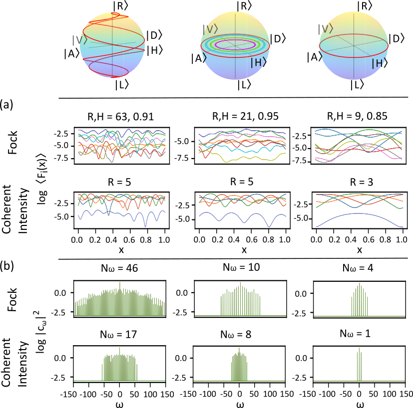
Figure 2: Photon-QuaRC, quantum and classical behavior for various encodings. Two different states and detection schemes are applied to the same $M=5$ network. Fock: A four-photon Fock state $|\vec{n}\rangle=|1,1,1,1,0\rangle$ with perfect PNR detection. Coherent Intensity: A four-port classical state $|\vec{\alpha}\rangle=|.5,.5,.5,.5,0\rangle$ with intensity detection at each port. (a) The first 10 most probable output functions for each case. (b) Corresponding Fourier spectra for each set of output functions. Each column corresponds to a different encoding scheme. Left: Spiral with $l_{m}=4m$. Center: Multi-linear where $l_{m}=m$. Right: Uniform-linear. The labels $R$ and $H$ refer to the rank and spectral entropy of the distribution respectively. $N_{\omega}$ denotes the number of elements in a spectrum excluding redundant negative frequencies and the DC component.

Encoding schemes. The expressive power of a network is determined by the encoding scheme and the input state. While an exhaustive investigation of all possible encodings and input states is outside the scope of this work, we will discuss a few schemes here, also shown in the top row of Fig. 2 (see the SM for more details).

Uniform linear: The first and simplest encoding is one in which all photons are given the same linear polarisation angle $\theta\in[0,2\pi]$ which traverses one equatorial orbit over the data domain, $\theta=lx$.

Multi-slope linear: As the uniform linear scheme is ultimately limited by the number of photons, it is natural to try to broaden the spectrum by encoding multiple frequencies directly in each port. One method is to apply a different linear function to the polarisation of each photon $\theta_{m}=l_{m}x$.

Spiral: By including elliptical polarisations such that our data are encoded in both $\theta$ and $\phi$ in Eq. (5) we can design encodings with useful properties inherited from the topology of the Poincaré sphere. A natural geometry is a spiral which traverses the sphere from pole to pole and returns to form a closed curve. This encoding can undergo an arbitrary number of azimuthal revolutions $l_{m}$ over the domain of the data while also providing low-frequency content from the zenith traversal.

Figure 2 displays the output functions and frequency spectrum generated by several different encoding schemes for both a four photon Fock state with PNR detection as well as a four port coherent state with intensity detection. We can see that the choice of encoding can tune the rank, distribution and spectrum of the output. In the Fock case we can see that adding complexity to the encoding trajectory increases the size of the Fourier spectrum as well as the rank and spectral entropy of the output. This in turn, improves the expressivity of the system. In contrast, the rank of the classical case - coherent states with intensity detection - is limited to the number of output ports of the network and the Fourier spectrum grows much slower. This further serves to illustrate the scaling advantages gained through quantum resources. The change in frequency content with different encodings is evident in the curvature of the output functions in Fig. 2a where the spiral and multi-linear encodings bias the most probable functions to higher frequencies. It is important to note that choosing an encoding scheme which simply maximizes rank does not ensure optimal performance on a task. Encodings must be chosen in a principled manner to balance rank, spectral entropy, and frequency content based on the desired task.

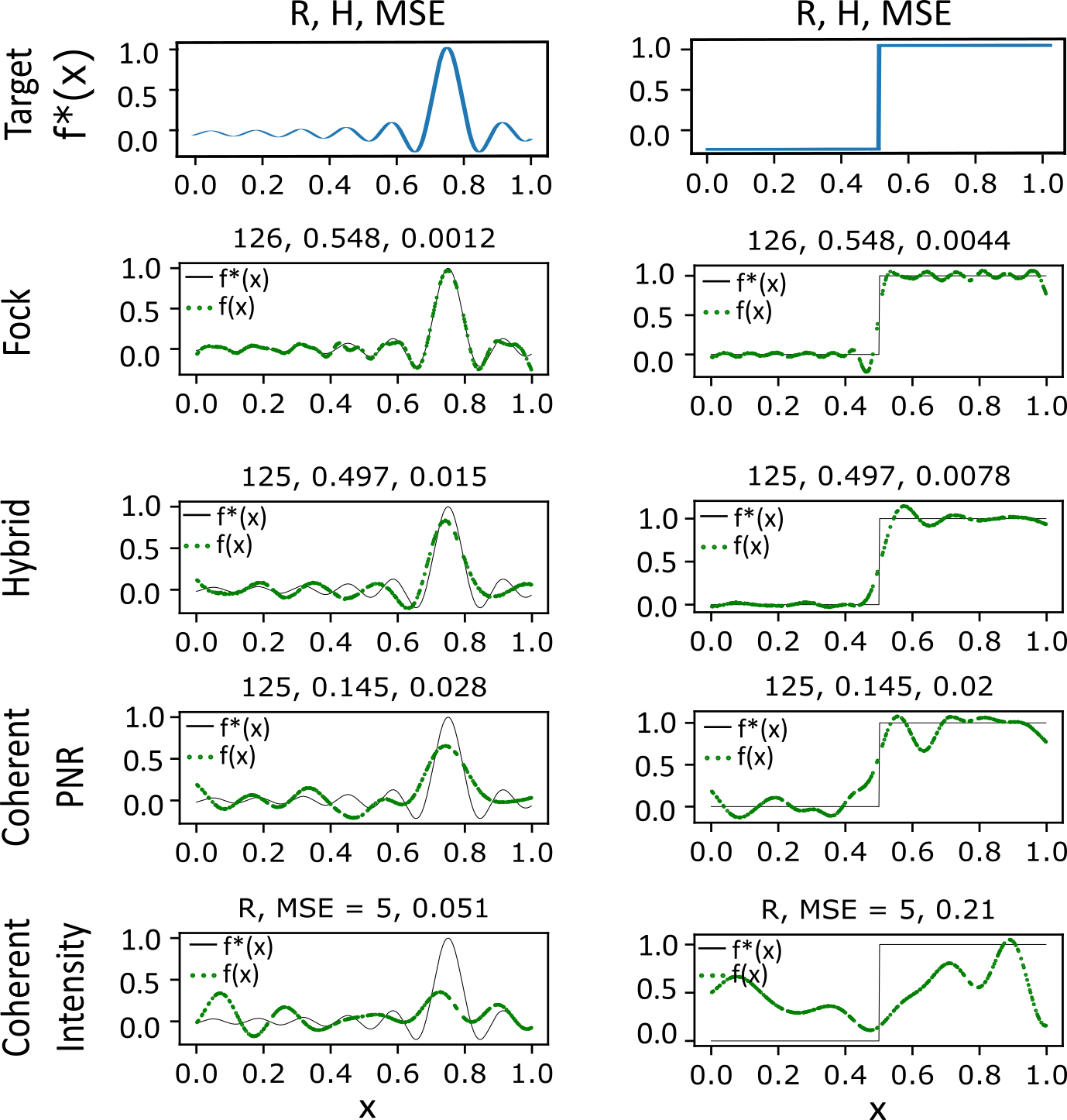
Figure 3: Function interpolation, comparing the approximation $f(x)$ to the target function $f^{*}(x)$. All trials use spiral encoding with $l_{m}=3m$ and post-selection on $\leq 4$ photon events with $\eta=.9$ and $N_{samp}=10^{7}$. Performance metrics [R,H,MSE] are listed in the title for each task/state combination. The states used are Fock: $|\vec{n}\rangle=|1,1,1,1,0\rangle$ with PNR detection, Hybrid: $|\psi_{\vec{\alpha},\vec{n}}\rangle=|0.5+1,0.5+1,0,0,0\rangle$ with PNR detection, Coherent PNR: $|\vec{\alpha}\rangle=|0.5,0.5,0,0,0\rangle$ with PNR detection, Coherent Intensity: Fully classical operation using $|\vec{\alpha}\rangle=|0.5,0.5,0.5,0.5,0\rangle$ with intensity detection. Each coherent state subject to PNR detection is approximated as a superposition of Fock states up to the sixth order. Each trial uses a 50/50 test/train data split.

Photon-QuaRC as a function interpolator. In Fig. 3 we demonstrate differences in performance between various implementations applied to machine learning tasks, e.g. function interpolation. The ultimate goal is to maximize performance for a fixed number of resources and to demonstrate each design under realistic conditions of operation.

We first define the target function $f^{*}(x)$ on an interval $x$, and discretize it to generate sets of data and labels, $\{x_{i},y_{i}\}$. These are randomly and uniformly split into two sets for training and validation, such that the device must learn the entire function in order to correctly interpolate it.

To simulate the output in real-world scenarios, accounting for limited sampling and imperfect detection, we employ a binomial model with a detector efficiency $\eta$. This model is applied to the ideal distribution $\langle\vec{F}(x)\rangle$. We then post-select the Fock subspace that corresponds to the detection events of interest while all other events are grouped into a non-detection state. After determining the final distribution, we draw a total number of samples $N_{samp}$ to simulate the process of injecting copies of the input state to build statistics. The training data are used to form the output matrix $O$ from which we extract the rank and spectral entropy. We then inject the validation data and apply a mean squared error (MSE) between the outputs and their corresponding labels to quantify the task performance.

Results. As shown in Fig. 3, there exists a clear improvement in performance and generalization as we increase the quantum resources. The details of this hierarchy for a specific function depend on the overlap of the output and target spectra. However, the correlation of MSE to the spectral entropy across vastly different target functions suggests that increasingly quantum sources are more robust under realistic conditions of operation due to higher uniformity in the output distribution over singular values (see SM for more details). We can see that the Fock state input yields the lowest error for both the sinc and step function interpolation. This is because the definite photon number ensures that the four-photon amplitudes in $\langle\vec{F}(x)\rangle$ are most probable and well-sampled. The hybrid states display better performance and generalization across tasks relative to the coherent states for similar reasons as the addition of the single photons reduces the uncertainty in photon number. However, as the higher-photon terms are less probable than with Fock states, hybrid states display a larger MSE for each task. Beyond the clear increase in performance with quantum resources at the input, we also note that in all cases we see an increase in performance related to photon number-resolving detection at the output: this alone grants an advantage over the fully classical case (i.e. coherent states sampled without PNR detection) due to the scaling of the output space. A discussion of how particular states were chosen for comparison may be found in the SM.

Conclusions. We have presented an approach to QML that is based on a linear photonic network. This shows an advantage when using quantum resources, with PNR detection as the minimal quantum resource which alone yields improvement over the tested classical measurements. Beyond the use of PNR, we also show a further hierarchical improvement of the QRC with increasing quantum resources at the input where performance increases from coherent to hybrid to pure Fock states. The reservoir architecture allows the device to be realized with simple optical systems, such as multimode fibers, and saves time and energy in the training stage. In this work we demonstrated the performance for function interpolation. Although it can also be used for classification, we feel that the method is best suited to tasks in which data encoded in quantum states are mapped to functions of a small number of variables. One example would be as integrated quantum information processing units in communication networks performing tasks such as quantum state tomography. Future work will focus on developing further optimized encoding schemes and design alterations to allow for time-series prediction.

References

- Biamonte et al. [2017] J. Biamonte, P. Wittek, N. Pancotti, P. Rebentrost, N. Wiebe, and S. Lloyd, Nature 549, 195 (2017).
- Ghosh et al. [2019] S. Ghosh, A. Opala, M. Matuszewski, T. Paterek, and T. C. Liew, npj Quantum Information 5, 10.1038/s41534-019-0149-8 (2019).
- [3] H.-Y. Huang, M. Broughton, J. Cotler, S. Chen, J. Li, M. Mohseni, H. Neven, R. Babbush, R. Kueng, J. Preskill, and J. R. Mcclean, Science 17, 2023.
- Wang et al. [2019] H. Wang, J. Qin, X. Ding, M. C. Chen, S. Chen, X. You, Y. M. He, X. Jiang, L. You, Z. Wang, C. Schneider, J. J. Renema, S. Höfling, C. Y. Lu, and J. W. Pan, Physical Review Letters 123, 10.1103/PhysRevLett.123.250503 (2019).
- Madsen et al. [2022] L. S. Madsen, F. Laudenbach, M. F. Askarani, F. Rortais, T. Vincent, J. F. Bulmer, F. M. Miatto, L. Neuhaus, L. G. Helt, M. J. Collins, A. E. Lita, T. Gerrits, S. W. Nam, V. D. Vaidya, M. Menotti, I. Dhand, Z. Vernon, N. Quesada, and J. Lavoie, Nature 606, 75 (2022).
- Arrazola et al. [2021] J. M. Arrazola, V. Bergholm, K. Brádler, T. R. Bromley, M. J. Collins, I. Dhand, A. Fumagalli, T. Gerrits, A. Goussev, L. G. Helt, J. Hundal, T. Isacsson, R. B. Israel, J. Izaac, S. Jahangiri, R. Janik, N. Killoran, S. P. Kumar, J. Lavoie, A. E. Lita, D. H. Mahler, M. Menotti, B. Morrison, S. W. Nam, L. Neuhaus, H. Y. Qi, N. Quesada, A. Repingon, K. K. Sabapathy, M. Schuld, D. Su, J. Swinarton, A. Száva, K. Tan, P. Tan, V. D. Vaidya, Z. Vernon, Z. Zabaneh, and Y. Zhang, Nature 591, 54 (2021).
- Bogaerts et al. [2020] W. Bogaerts, D. Pérez, J. Capmany, D. A. Miller, J. Poon, D. Englund, F. Morichetti, and A. Melloni, Programmable photonic circuits (2020).
- Luo et al. [2023] W. Luo, L. Cao, Y. Shi, L. Wan, H. Zhang, S. Li, G. Chen, Y. Li, S. Li, Y. Wang, S. Sun, M. F. Karim, H. Cai, L. C. Kwek, and A. Q. Liu, Recent progress in quantum photonic chips for quantum communication and internet (2023).
- Kjaergaard et al. [2020] M. Kjaergaard, M. E. Schwartz, J. Braumüller, P. Krantz, J. I.-J. Wang, S. Gustavsson, and W. D. Oliver, Annual Review of Condensed Matter Physics 11, 369 (2020), https://doi.org/10.1146/annurev-conmatphys-031119-050605 .
- McMahon [2023] P. L. McMahon 10.1038/s42254-023-00645-5 (2023).
- Tan and Rohde [2019] S. H. Tan and P. P. Rohde, The resurgence of the linear optics quantum interferometer — recent advances and applications (2019).
- Gard et al. [2014] B. T. Gard, K. R. Motes, J. P. Olson, P. P. Rohde, and J. P. Dowling doi:10.1142/9789814678704_0008 (2014).
- Paivi Torma and Jex [1995] S. S. Paivi Torma and I. Jex, Physical Review A 52, 10.1103/physreva.52.4853 (1995).
- van der Meer et al. [2021] R. van der Meer, S. Huber, P. W. H. Pinkse, R. García-Patrón, and J. J. Renema, (2021).
- Broome et al. [2013] M. A. Broome, A. Fedrizzi, S. Rahimi-Keshari, J. Dove, S. Aaronson, T. C. Ralph, and A. G. White, Science 339, 794 (2013).
- Marcucci et al. [2020] G. Marcucci, D. Pierangeli, P. W. H. Pinkse, M. Malik, and C. Conti, Opt. Express 28, 14018 (2020).
- Wright et al. [2023] D. Wright, C. Igel, G. Samuel, and R. Selvan, (2023).
- Defienne et al. [2016] H. Defienne, M. Barbieri, I. A. Walmsley, B. J. Smith, and S. Gigan, Science Advances 2, 10.1126/sciadv.1501054 (2016).
- Rafayelyan et al. [2020] M. Rafayelyan, J. Dong, Y. Tan, F. Krzakala, and S. Gigan, Physical Review X 10, 10.1103/PhysRevX.10.041037 (2020).
- Tanaka et al. [2019] G. Tanaka, T. Yamane, J. B. Héroux, R. Nakane, N. Kanazawa, S. Takeda, H. Numata, D. Nakano, and A. Hirose, Neural Networks 115, 100 (2019).
- García-Beni et al. [2022] J. García-Beni, G. L. Giorgi, M. C. Soriano, and R. Zambrini 10.1103/PhysRevApplied.20.014051 (2022).
- Scheel [2004] S. Scheel, Permanents in linear optical networks (2004), arXiv:quant-ph/0406127 [quant-ph] .
- Gan et al. [2022] B. Y. Gan, D. Leykam, and D. G. Angelakis, EPJ Quantum Technology 9, 10.1140/epjqt/s40507-022-00135-0 (2022).
- Schuld et al. [2021] M. Schuld, R. Sweke, and J. J. Meyer, Physical Review A 103, 10.1103/PhysRevA.103.032430 (2021).
- Vidal and Theis [2020] F. J. G. Vidal and D. O. Theis, Frontiers in Physics 8, 10.3389/fphy.2020.00297 (2020).
- Afek et al. [2010] I. Afek, O. Ambar, and Y. Silberberg, Science 328, 879 (2010), https://www.science.org/doi/pdf/10.1126/science.1188172 .
- Windhager et al. [2010] A. Windhager, M. Suda, C. Pacher, M. Peev, and A. Poppe 10.1016/j.optcom.2010.12.019 (2010).
- Reck et al. [1994] M. Reck, A. Zeilinger, H. J. Bernstein, and P. Bertani, Experimental realization of any discrete unitary operator (1994).
- Thibeault et al. [2024] V. Thibeault, A. Allard, and P. Desrosiers, Nature Physics 10.1038/s41567-023-02303-0 (2024).