Distributed Safe Navigation of Multi-Agent Systems using Control Barrier Function-Based Optimal Controllers

Abstract

This paper proposes a distributed controller synthesis framework for safe navigation of multi-agent systems. We leverage control barrier functions to formulate collision avoidance with obstacles and teammates as constraints on the control input for a state-dependent network optimization problem that encodes team formation and the navigation task. Our algorithmic solution is valid for general nonlinear control dynamics and optimization problems. The resulting controller is distributed, satisfies the safety constraints at all times, and is asymptotically optimal. We illustrate its performance in a team of differential-drive robots in a variety of complex environments, both in simulation and in hardware.

I Introduction

Safety-critical control has received a lot of attention in the robotics and controls communities motivated by applications like autonomous driving, navigation of robotic swarms, and optimal power flow of energy grids, where safety constraints are ubiquitous. Control barrier functions (CBFs) are a computationally efficient tool for the synthesis of safe controllers. In scenarios involving multiple autonomous agents, safety constraints often couple the decisions of the different team members. The challenge we face then is how to extend the CBF framework to multi-agent settings in a distributed manner (i.e., with each agent designing its local controller using only information from neighboring agents) while still retaining its efficiency, safety, and optimality guarantees. This question serves as the main motivation for this paper.

Literature Review

This work draws on notions and techniques from the body of work pertaining to CBFs [1, 2], which are a powerful tool to render safe a given set. Formally, safe controllers can be synthesized [3] by incorporating CBF-based conditions as constraints in an optimization problem whose objective encodes desired specifications on the input. Such optimization problems have state-dependent constraints and need to be studied in feedback loop with a plant. This type of optimization-based controllers have been well-studied in the literature [4, 5, 6, 7]. Often, these problems cannot be solved instantaneously and instead approximate controllers must be implemented in closed-loop. Here, we draw on ideas from the “dynamical systems approach to algorithms” that views optimization algorithms as continuous-time dynamical systems, cf. [8, 9], which is a useful perspective when implementing optimization-based controllers in feedback systems [4, 5, 10, 11, 12]. In the context of multi-agent systems, many applications require a distributed implementation of the individual agents’ controllers. For optimization-based controllers resulting from CBFs, this requires a distributed solution of the resulting optimization problem. The works [13, 14, 15] tackle this problem for QPs by splitting a centralized QP into local QPs that can be solved efficiently while preserving safety guarantees. However, the solution of these local QPs might lack optimality guarantees with respect to the original QP. The recent works [16, 17] introduce different algorithms to solve constrained optimization problems in a distributed fashion while satisfying the constraints throughout the execution of the algorithm. However, [16] is restricted to a class of parametric QPs with uniformly bounded coefficients and our work [17] does not consider the implementation of the optimization problem in feedback loop with a plant.

Statement of Contributions

We design a distributed controller for safe navigation of multi-agent systems. We propose a synthesis framework which leverages CBFs to formulate obstacle avoidance and inter-agent collision avoidance constraints as affine inequalities in the control input. These constraints are included in a state-dependent network optimization problem that finds the control inputs allowing the agents to reach different waypoints of interest while maintaining a given formation and satisfying the safety constraints. Our first contribution leverages the particular structure of the optimization problem to decouple its constraints by using a set of auxiliary constraint mismatch variables while still keeping the same feasible set. This enables us to derive a distributed update law for these auxiliary variables that allows each agent to obtain its local control input by solving a local optimization problem without the need to coordinate with any other agent. Our second contribution establishes that the proposed controller design is distributed, safe, and asymptotically optimal. Our last contribution is the implementation of the proposed controller in a variety of different environments, robots and formations, both in simulation and in real hardware.

II Preliminaries

We introduce here basic notation and preliminaries on CBFs, constrained optimization, and projected saddle-point dynamics. This section can be safely skipped by a reader already familiar with these notions.

Notation

We denote by and _>0 the set of real and nonnegative real numbers, respectively. For a positive integer $n$, we let $[n]=\{1,\ldots,n\}$. Given a set $A$, $|A|$ denotes its cardinality. Given $x\in^{n}$, $\lVert x\rVert$ denotes its Euclidean norm. For $a\in$ and $b\in_{\geq 0}$, we let

$$[a]_{b}^{+}=\begin{cases}a,\quad&\text{if}\ b>0,\\ \max\{0,a\},\quad&\text{if}\ b=0.\end{cases}$$

For vectors $a\in^{n}$ and $b\in_{\geq 0}^{n}$, $[a]_{b}^{+}$ denotes the vector whose $i$-th component is $[a_{i}]_{b_{i}}^{+}$, for $i\in[n]$. Given a set $\mathcal{P}\subseteq^{n}$ and variables $\xi=\{x_{i_{1}},x_{i_{2}},\dots,x_{i_{k}}\}$, we denote by $\Pi_{\xi}\mathcal{P}=\{(x_{i_{1}},x_{i_{2}},\dots,x_{i_{k}})\in^{k}\;:\;x\in\mathcal{P}\}$ the projection of $\mathcal{P}$ onto the $\xi$ variables. An undirected graph is a pair $\mathcal{G}=(V,\mathcal{E})$, where $V=V(\mathcal{G})=\{1,\ldots,N\}$ is the vertex set and $\mathcal{E}=\mathcal{E}(\mathcal{G})\subseteq V\times V$ is the edge set, with $(i,j)\in\mathcal{E}$ if and only if $(j,i)\in\mathcal{E}$. The set of neighbors of node $i$ is $\mathcal{N}_{i}=\{j\in V\;:\;(i,j)\in\mathcal{E}\}$. For a real-valued function $f:^{n}\times^{m}\to$, we denote by $\nabla_{x}f$ and $\nabla_{y}f$ the column vectors of partial derivatives of $f$ with respect to the first and second arguments, respectively. Let $F:^{n}\to^{n}$ be locally Lipschitz and consider the dynamical system $\dot{x}=F(x)$. A set $\mathcal{C}$ is forward invariant for $\dot{x}=F(x)$ if all trajectories that start in $\mathcal{C}$ remain in $\mathcal{C}$ for all positive times.

Control Barrier Functions

Consider the control-affine system

$$\dot{x}=F(x)+G(x)u$$ (1)

where $F:^{n}\rightarrow^{n}$ and $G:^{n}\to^{n\times m}$ are locally Lipschitz functions, with $x\in^{n}$ the state and $u\in^{m}$ the input. Let $\mathcal{C}\subset^{n}$ and $h:^{n}\to$ be a continuously differentiable function such that

$$\mathcal{C} =\{x\in^{n}\;:\;h(x)\geq 0\},$$ (2a)

$$\partial\mathcal{C} =\{x\in^{n}\;:\;h(x)=0\}.$$ (2b)

The function $h$ is a control barrier function (CBF) [1, Definition 2] of $\mathcal{C}$ if there exists a $\mathcal{K}_{\infty}$ function $\alpha$ such that for all $x\in\mathcal{C}$, there exists $u\in^{m}$ with

$$L_{F}h(x)+L_{G}h(x)u+\alpha(h(x))\geq 0.$$ (3)

A Lipschitz controller $k:^{n}\to^{m}$ such that $u=k(x)$ satisfies (3) for all $x\in\mathcal{C}$ makes $\mathcal{C}$ forward invariant. Hence, CBFs provide a way to guarantee safety.

Projected Saddle-Point Dynamics

Given continuously differentiable functions $f:^{n}\to$ and $g:^{n}\to^{p}$, whose derivatives are locally Lipschitz, consider the constrained nonlinear program

$$\min\limits_{x\in^{n}}f(x)$$ (4)

$$\text{s.t.}\quad g(x)\leq 0.$$

Let $\mathcal{L}:^{n}\times^{p}_{\geq 0}$ be its associated Lagrangian, $\mathcal{L}(x,\lambda)=f(x)+\lambda^{T}g(x)$. The projected saddle-point dynamics for $\mathcal{L}$ are defined as follows:

$$\dot{x} =-\nabla_{x}\mathcal{L}(x,\lambda,\mu),$$ (5a)

$$\dot{\lambda} =[\nabla_{\lambda}\mathcal{L}(x,\lambda,\mu)]_{\lambda}^{+}.$$ (5b)

If $f$ is strongly convex and $g$ is convex, then $\mathcal{L}$ has a unique saddle point, which corresponds to the KKT point of (4). Moreover, [18, Theorem 5.1] ensures that it is globally asymptotically stable under the dynamics (5).

Constraint Mismatch Variables

Consider a network composed by agents $\{1,\ldots,N\}$ whose communication topology is described by a connected undirected graph $\mathcal{G}$. An edge $(i,j)$ represents the fact that agent $i$ can receive information from agent $j$ and vice versa. For each $i\in[N]$ and $k\in[p]$, let $f_{i}:^{n}\to$ be a strongly convex function and $g_{i}^{k}:^{n}\rightarrow$ a convex function. We consider the following optimization problem with separable objective function and constraints

$$\min\limits_{u\in^{nN}}\sum_{i=1}^{N}f_{i}(u_{i})$$ (6)

$$\text{s.t.}\quad\sum_{i\in V(\mathcal{G}_{k})}g_{i}^{k}(u_{i})\leq 0,\quad k\in[p],$$

where $\mathcal{G}_{k}$ is a connected subgraph of $\mathcal{G}$ for each $k\in[p]$. For each $k\in[p]$, the constraint in (6) couples the local variable $u_{i}$ of agent $i$ with the variables of all the other agents in $\mathcal{G}_{k}$. The constraints in (6) can be decoupled by introducing constraint-mismatch variables [19, 17], which help agents keep track of local constraints while ensuring that the original constraints are collectively satisfied. Specifically, we add one constraint-mismatch variable per agent and constraint. We let $z_{i}^{k}\in$ be the constraint-mismatch variable for agent $i$ and constraint $k$. Let $P_{i}:=\{k\in[p]\;:\;i\in V(\mathcal{G}_{k})\}$ be the set of indices of the constraints in which agent $i$ is involved. For convenience, we use the notation $u=[u_{1},\ldots,u_{N}]$, $z_{i}=\{z_{i}^{k}\}_{k\in P_{i}}$, $z=[z_{1},\ldots,z_{N}]$ and $q:=\sum_{i=1}^{N}|P_{i}|$. Next, consider the problem

$$\min\limits_{u\in^{nN},\ z\in^{q}}\sum_{i=1}^{N}f_{i}(u_{i})$$ (7)

$$\text{s.t.}\quad g_{i}^{k}(u_{i})+\sum_{j\in\mathcal{N}_{i}\cap\mathcal{G}_{k}}(z_{i}^{k}-z_{j}^{k})\leq 0,\quad i\in\mathcal{G}_{k},\ k\in[p].$$

In (7), the constraints are now locally expressible, meaning that agent $i\in[N]$ can evaluate the ones in which its variable $u_{i}$ is present by using variables obtained from its neighbors. The next result establishes the equivalence of (6) and  (7).

Proposition II.1

(Equivalence between the two formulations): Let $\mathcal{F}^{*}$ be the solution set of (7). Then, $u^{*}=\Pi(\mathcal{F}^{*})$ is the optimizer of (6).

The proof is similar to [17, Proposition 4.1], with the necessary modifications to account for the fact that the constraints of (6) might only involve a subset of the agents.

III Problem Statement

We are interested in designing distributed controllers that allow a team of differential-drive robots to safely navigate an environment while maintaining a certain desired formation and visiting a sequence of waypoints of interest. The robots have identities $\{1,\ldots,N\}$ and follow unicycle dynamics

$$\dot{x}_{i}=v_{i}\cos{\theta_{i}},\quad\dot{y}_{i}=v_{i}\sin{\theta_{i}},\quad\dot{\theta_{i}}=\omega_{i},$$ (8)

where $s_{i}=[x_{i},y_{i}]\in^{2}$ is the position of agent $i$, $\theta_{i}\in[0,2\pi)$ its heading and $v_{i}\in$ and $w_{i}\in$ are its linear and angular velocity control inputs, respectively.

We next leverage the notion of CBFs to encode the different safety specifications, giving rise to affine constraints in the control inputs. We note that, under the dynamics (8), direct application of (3) on functions that only depend on position results in limited design flexibility because $\omega_{i}$ does not appear in the time derivative of $s_{i}$. Instead, we follow [20, Section IV] and define, for all $i\in[N]$,

$$R(\theta_{i})\!=\!\begin{bmatrix}\cos{\theta_{i}}&\!-\sin{\theta_{i}}\\ \sin{\theta_{i}}&\!\cos{\theta_{i}}\end{bmatrix},\ p_{i}\!=\!s_{i}\!+\!lR(\theta_{i})e_{1},\ L\!=\!\begin{bmatrix}1&\!0\\ 0&\!1/l\end{bmatrix}$$

where $e_{1}=[1,0]^{T}$ and $l>0$ is a design parameter. This defines $p_{i}$ as a point orthogonal to the wheel axis of the robot. It follows that $\dot{p}_{i}=R(\theta_{i})L^{-1}u_{i}$, where $u_{i}=[v_{i},w_{i}]^{T}$. Hence, by choosing $p_{i}$ as our position variable, both control inputs appear in the time derivative of the position, which allows for more flexibility in our control design.

Avoiding obstacles

We consider an environment with $M$ obstacles $\{\mathcal{O}_{k}\}_{k\in[M]}$, each of them expressable as the sublevel set of a differentiable function $h_{k}$, i.e., $\mathcal{O}_{k}=\{(x,y)\in^{2}\;:\;h_{k}(x,y)<0\}$. To guarantee that the robot does not collide with the obstacles, we want to ensure that

$$h_{k}(p_{i})\geq\eta_{k}>0,\quad\forall k\in[M].$$ (9)

The parameter $\eta_{k}\in$ should be taken large enough to guarantee that the whole physical robot (instead of just $p_{i}$) does not collide with the obstacle $\mathcal{O}_{k}$. For instance, if $r_{i}$ is the radius of robot $i$ and $\mathcal{O}_{k}$ is a circular obstacle with center at $m_{k}\in^{2}$ and radius $R_{k}$ so that $h_{k}(p_{i})=\lVert p_{i}-m_{k}\rVert^{2}-R_{k}^{2}$, then $\eta_{k}$ can be taken as $(r_{i}+l)^{2}+2R_{k}(r_{i}+l)$. The CBF condition associated with (9) with linear class $\mathcal{K}_{\infty}$ function with slope $\alpha_{k}>0$ reads

$$\nabla h_{k}(p_{i})^{T}R(\theta_{i})L^{-1}u_{i}\geq-\alpha_{k}(h_{k}(p_{i})-\eta_{k}).$$ (10)

Avoiding inter-agent collisions

We also want to enforce that agents do not collide with other team members. To achieve this, we assume it is enough for each robot $i$ to avoid colliding with a subset of the agents $N_{i}\subset[N]\backslash\{i\}$. This is motivated by the fact that our control design will make the team maintain a certain formation at all times, meaning that each agent only needs to avoid colliding with agents closest to it in the formation. For this reason, we assume that if $j\in N_{i}$, then $i\in N_{j}$, and that agent $i$ can communicate with all agents in $N_{i}$ to obtain their state variables. We assume that the resulting communication graph is connected. For any $i\in[N]$ and $j\in N_{i}$, we want to ensure

$$d(p_{i},p_{j}):=\lVert p_{i}-p_{j}\rVert^{2}-d_{\text{min}}^{2}\geq 0,$$ (11)

with $d_{\text{min}}\geq r_{i}+r_{j}+2l$. The CBF condition for (11) with a linear class $\mathcal{K}_{\infty}$ function with slope $\alpha_{c}^{ij}>0$ reads

$$(p_{i}\!-\!p_{j})^{T}(R(\theta_{i})L^{-1}u_{i}\!-\!R(\theta_{j})L^{-1}u_{j})\geq-\alpha_{c}^{ij}d(p_{i},p_{j}).$$ (12)

Team formation

Finally, we are interested in making the team reach a goal while maintaining a certain formation. To do so, we define a leader for the team (without loss of generality, agent $1$). The rest of the agents $\{2,\ldots,N\}$ are referred to as followers. The leader is in charge of steering the team towards a given waypoint $q_{1}\in^{2}$. To achieve it, we define a nominal controller $u_{\text{nom},1}:^{2}\to^{2}$ that steers it towards $q_{1}$. We use the stabilizing controller for the unicycle dynamics in [21]. To define it, let $e_{1}:^{2}\to$ and $\beta_{1}:^{2}\to$ defined as

$$e_{1}(p_{1}) =\sqrt{(p_{1,x}-q_{1,x})^{2}+(p_{1,y}-q_{1,y})^{2}},$$

$$\beta_{1}(p_{1}) =\arctan\Big{(}\frac{p_{1,y}-q_{1,y}}{p_{1,x}-q_{1,x}}\Big{)}.$$

The control law is $u_{\text{nom},1}(p_{1})=[v_{1}(p_{1}),w_{1}(p_{1})]$, where

$$v_{1}(p_{1}) =k_{r}e(p_{1})\cos(\beta_{1}(p_{1}))-\theta_{1}),$$ (13a)

$$\omega_{1}(p_{1}) =k_{a}\beta_{1}(p_{1})+\frac{k_{r}}{2}\sin(2\beta_{1}(p_{1}))\frac{\beta_{1}(p_{1})\!+\!h\theta_{1}}{\beta_{1}(p_{1})},$$ (13b)

and $k_{r}>0,k_{a}>0$ and $h>0$ are design parameters. We can also specify a sequence of waypoints for the leader: once the leader is within a certain tolerance of the current desired waypoint, $u_{\text{nom},1}$ can be updated to steer the leader towards the next desired waypoint.

As the leader moves towards the desired waypoint, the followers follow it while maintaining a certain formation of interest. We define the desired formation positions for the followers as follows. First, recall that $N_{1}:=\{i\in[N]\backslash\{1\}\;:\;i\ \text{and}\ 1\ \text{are connected}\}$ and, for $k\in\mathbb{Z}_{>0}$, $k>1$, define the $k$-neighborhood of the leader as $N_{1}^{k}:=\{i\in[N]\;:\;\exists\ j\in N_{1}^{k-1}\ \text{s.t.}\ i\in N_{j}\}$. Since the communication graph is connected, there exists $K\in\mathbb{Z}_{>0}$ such that, for all $i\in[N]\backslash\{1\}$, there is $k\in[K]$ such that $i\in N_{1}^{k}$. For every $i\in[N]\backslash\{1\}$, we let $k_{i}$ be the smallest positive integer $k$ such that $i\in N_{1}^{k}$. For every $i\in[N]\backslash\{1\}$, we consider functions $q_{i}:^{2|N_{1}^{k_{i}-1}\cap N_{i}|}\to^{2}$ such that $q_{i}(\{p_{j}\}_{j\in N_{1}^{k_{i}-1}\cap N_{i}})$ defines the desired formation position for agent $i$. Agent $i$ aims to remain as close as possible to $q_{i}(\{p_{j}\}_{j\in N_{1}^{k_{i}-1}\cap N_{i}})$ while maintaining the safety constraints. To achieve this, we define a nominal controller $u_{\text{nom},i}:^{2}\to^{2}$ for each agent $i\in\{2,\ldots,N\}$ analogous to (13) that steers it towards its desired formation position $q_{i}(\{p_{j}\}_{j\in N_{1}^{k_{i}-1}\cap N_{i}})$. Note that $q_{i}$ can be computed in a distributed fashion because it only depends on the positions of agents in $N_{1}^{k_{i}-1}\cap N_{i}\subset N_{i}$.

Agents collectively try to design controllers $u_{i}$ for all $i\in[N]$ that satisfy the obstacle avoidance and inter-agent collision avoidance safety constraints while remaining as close as possible to their corresponding nominal controller. By employing weighting matrix-valued functions $\Gamma_{i}:^{n}\to^{m\times m}$ for each $i\in[N]$ that can be designed to penalize the linear and angular velocity inputs differently, and leveraging the CBF conditions (10), (12), we obtain the following network-wide optimization problem:

$$\min\limits_{\{u_{i}\in^{2}\}_{i=1}^{N}}\quad\sum_{i=1}^{N}\frac{1}{2}\lVert\Gamma_{i}(p_{i})(u_{i}-u_{\text{nom},i}(p_{i}))\rVert^{2}$$ (14)

$$\text{s.t.}\ (p_{i}-p_{j})^{T}(R(\theta_{i})L^{-1}u_{i}-R(\theta_{j})L^{-1}u_{j})\geq-\alpha_{c}^{ij}d(p_{i},p_{j}),$$

$$\qquad\qquad\qquad\qquad\qquad\qquad i\in[N],\ j\in N_{i},$$

$$\quad\nabla h_{k}(p_{i})^{T}R(\theta_{i})L^{-1}u_{i}\geq-\alpha_{k}(h_{k}(p_{i})-\eta_{k}),$$

$$\qquad\qquad\qquad\qquad\qquad\qquad i\in[N],\ k\in[M].$$

The inter-agent collision avoidance constraints (12) require coordination between agents involved in the constraint. This, together with the state-dependency of the objective function and constraints, poses challenges in the implementation of a distributed algorithm that solves (14). Our goal is to leverage its structure to design a distributed controller satisfying the constraints at all times, and such that it has the same optimality properties as the solution obtained directly from (14).

IV Distributed Controller Design

In this section we design a distributed algorithmic solution to the problem formulated in Section III. As it turns out, our solution is valid for a more general setup, as we explain next. Assume that the agents’ communication network is described by a connected undirected graph $\mathcal{G}$, as in Section III. An edge $(i,j)$ represents the fact that agent $i$ can receive information from agent $j$ and vice versa. We describe the dynamics of each agent $i\in[N]$ by

$$\dot{\xi}_{i}=F_{i}(\xi_{i},u_{i})$$ (15)

where $F_{i}:^{n}\times^{m}\to^{n}$ is a locally Lipschitz function for each $i\in[N]$, $\xi_{i}\in^{n}$ is the state variable of agent $i$ and $u_{i}\in^{m}$ is its local control input. Additionally, let $f_{i}:^{n}\times^{m}\to$ and $g_{i}^{k}:^{n|\mathcal{N}_{i}|}\times^{m}\to$, with $i\in[N]$ and $k\in[p]$ be continuously differentiable functions with Lipschitz derivatives. We assume that for all $i\in[N]$ and $\xi_{i}\in^{n}$, the functions $f_{i}(\xi_{i},\cdot)$ are strongly convex, and for all $i\in[N]$, $k\in[p]$ and $y_{i}\in^{n|\mathcal{N}_{i}|}$, the functions $g_{i}^{k}(y_{i},\cdot)$ are convex. The agents need to coordinate to solve an optimization problem of the form

$$\min\limits_{{\{u_{i}\in^{m}\}_{i=1}^{N}}}\sum_{i=1}^{N}f_{i}(\xi_{i},u_{i}),$$ (16)

$$\qquad\text{s.t.}\sum_{i\in V(\mathcal{G}_{k})}g_{i}^{k}(\xi_{\mathcal{N}_{i}},u_{i})\leq 0,\quad k\in[p].$$

where $\xi_{\mathcal{N}_{i}}=\{\xi_{j}\}_{j\in\mathcal{N}_{i}}$ and $\mathcal{G}_{k}$ is a connected subgraph of $\mathcal{G}$ for each $k\in[p]$. Note that (14) is a particular case of (16), where $f_{i}(\xi_{i},u_{i})=\frac{1}{2}\lVert\Gamma_{i}(\xi_{i})(u_{i}-u_{\text{nom},i}(\xi_{i}))\rVert^{2}$ and $\mathcal{G}_{k}$ corresponds to the graph with nodes $\{i\}\cup\{j\}$ and an edge between $\{i\}$ and $\{j\}$ for the inter-agent collision avoidance constraint between agent $i$ and $j$, and $\mathcal{G}_{k}$ corresponds to the singleton $\{k\}$ for the obstacle avoidance constraints of agent $k$. Moreover, $g_{i}^{k}$ takes the form of the corresponding CBF constraint in each case. Problem (16) can encode other types of safety constraints and more general dynamics. We henceforth denote $\xi=[\xi_{1},\ldots,\xi_{N}]\in^{nN}$ and $u=[u_{1},\ldots,u_{N}]\in^{mN}$. We assume that (16) is feasible.

Assumption 1

Problem (16) is feasible for all $\xi\in^{nN}$.

Assumption 1 is necessary for the solution of (16) to be well defined. If the constraints of (16) are defined by CBFs, such as those in (14), their joint feasibility can be characterized, cf. [22, 23].

We let $u^{*}:^{nN}\to^{mN}$ be the function mapping each $\xi\in^{nN}$ to the solution of (16).

To tackle the design of our distributed algorithm, we first deal with the coupling induced by the inequality constraints by introducing constraint mismatch variables $z_{i}^{k}$ for each agent and constraint in which it is involved. We use the same notation as in Section II and reformulate (16) as

$$\min\limits_{u\in^{mN},z\in^{q}}\sum_{i=1}^{N}f_{i}(\xi_{i},u_{i}),$$ (17)

$$\text{s.t.}\quad g_{i}^{k}(\xi_{\mathcal{N}_{i}},u_{i})+\!\!\!\!\!\!\!\sum_{j\in\mathcal{N}_{i}\cap V(\mathcal{G}_{k})}\!\!\!\!(z_{i}^{k}\!-\!z_{j}^{k})\leq 0,\ i\!\in\!V(\mathcal{G}_{k}),\ k\!\in\![p].$$

In order to facilitate the analysis of the convergence properties of the algorithms that will follow, we regularize (17) by adding the term $\epsilon\sum_{k=1}^{p}\sum_{j\in V(\mathcal{G}_{k})}(z_{j}^{k})^{2}$, with $\epsilon>0$, in the objective function of (17). Details regarding this regularization are covered in the Appendix. With the added regularization term, the problem (17) has a strongly convex objective function and convex constraints, and therefore has a unique optimizer for every $\xi\in^{nN}$. Let $u^{*,\epsilon}:^{nN}\to^{mN}$ and $z^{*,\epsilon}:^{nN}\to^{q}$ be the functions mapping each $\xi\in^{nN}$ to the corresponding unique optimizers in $u$ and $z$, respectively, of the regularized problem. We also let $\lambda^{*,\epsilon}:^{nN}\to^{q}$ be the function mapping each $\xi\in^{nN}$ to the optimal Lagrange multiplier of the regularized problem. Problem (17) (or its regularized version) cannot be decoupled into $N$ local optimization problems because the optimal values of $z$ in (17) require coordination among agents. However, for every fixed $z$, (17) can be solved locally by agent $i$ by just optimizing over $u_{i}$ as follows:

$$\min\limits_{u_{i}\in^{m}}f_{i}(\xi_{i},u_{i}),$$ (18)

$$\text{s.t.}\quad g_{i}^{k}(\xi_{\mathcal{N}_{i}},u_{i})+\sum_{j\in\mathcal{N}_{i}\cap V(\mathcal{G}_{k})}(z_{i}^{k}-z_{j}^{k})\leq 0,\quad\ k\in[p].$$

We let $\bar{u}_{i}:^{n|\mathcal{N}_{i}|}\times^{|\mathcal{N}_{i}|}$ be the function that maps every $(\xi_{\mathcal{N}_{i}},z_{\mathcal{N}_{i}})\in^{n|\mathcal{N}_{i}|}\times^{\sum_{j\in\mathcal{N}_{i}}|P_{j}|}$ to the optimizer of (18), and $\bar{u}=[\bar{u}_{1},\ldots,\bar{u}_{N}]$. By construction, the controller $\bar{u}_{i}$ is distributed, as it only depends on variables which can be obtained through communication with agents in $\mathcal{N}_{i}$.

However, $\bar{u}_{i}$ depends on the chosen value of $z$. Since (17) contains a minimization over both $u$ and $z$, in order to ensure that $\bar{u}_{i}$ coincides with the optimizer over $u$ of (17), one must also optimize over the constraint mismatch variables $z$. We do this by updating them with the projected saddle-point dynamics of the regularization of (17). This scheme is illustrated in Figure 1.

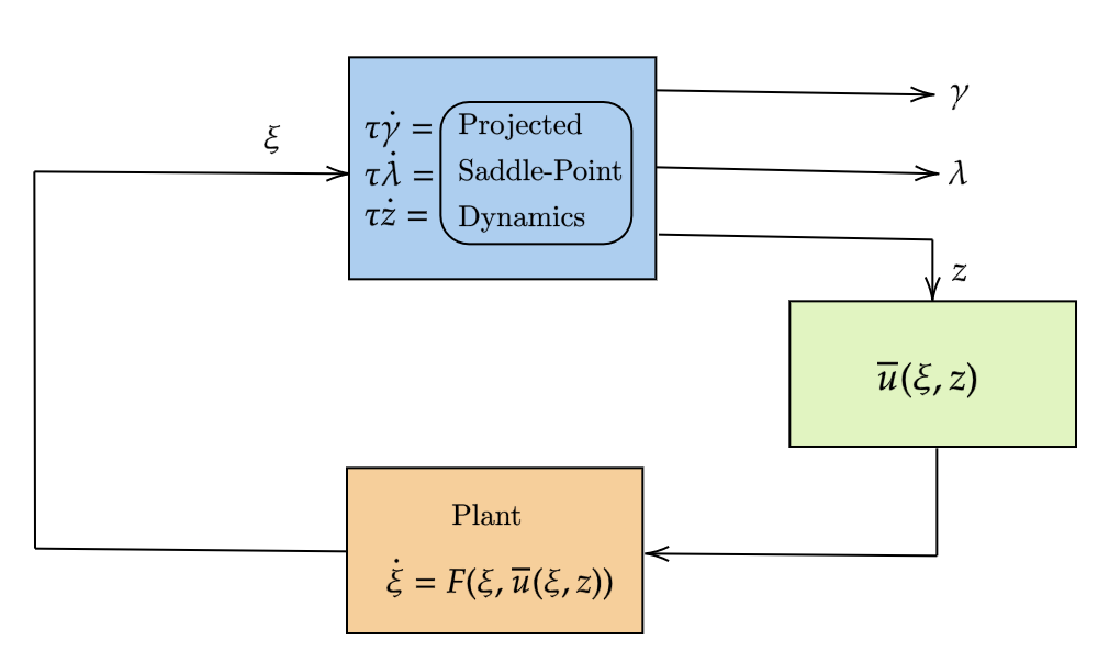
Figure 1: Block diagram of (19). The blue block updates the variables $\gamma$, $z$ and $\lambda$ using the projected saddle-point dynamics of the regularized version of (17). In parallel, the plant is updated using the controller $\bar{u}$.

We assume that the projected saddle-point dynamics can be run at a faster rate than the plant. Introducing a timescale separation parameter $\tau>0$ to model this, the interconnection of the projected saddle-point dynamics with the plant leads to the following dynamical system:

$$\tau\dot{\gamma}_{i} =-\nabla_{\gamma_{i}}f_{i}(\xi_{i},\gamma_{i})-\sum_{\{k\in[p]\;:\;i\in\mathcal{G}_{k}\}}\lambda_{i}^{k}\nabla_{\gamma_{i}}g_{i}^{k}(\xi_{\mathcal{N}_{i}},\gamma_{i}),~{}$$ (19a)

$$\tau\dot{z}_{i}^{k} =-\epsilon z_{i}^{k}-\sum_{j\in\mathcal{N}_{i}\cap\mathcal{G}_{k}}(\lambda_{i}^{k}-\lambda_{j}^{k}),~{}$$ (19b)

$$\tau\dot{\lambda}_{i}^{k} =[g_{i}^{k}(\xi_{\mathcal{N}_{i}},\gamma_{i})+\sum_{j\in\mathcal{N}_{i}\cap\mathcal{G}_{k}}(z_{i}^{k}-z_{j}^{k})]_{\lambda_{i}^{k}}^{+}~{},$$ (19c)

$$\dot{\xi}_{i} =F_{i}(\xi_{i},\bar{u}_{i}(\xi_{i},z_{\mathcal{N}_{i}})),~{}$$ (19d)

for all $i\in[N]$ and $k\in P_{i}$. We henceforth denote $\gamma=[\gamma_{1},\ldots,\gamma_{N}]$, $\lambda_{i}=\{\lambda_{i}^{k}\}_{k\in P_{i}}$ for all $i\in[N]$ and $\lambda=[\lambda_{1},\ldots,\lambda_{N}]$. Hence, our proposed algorithmic solution is the controller $\bar{u}_{i}$ for all $i\in[N]$ implemented for the current value of the state variables $\xi_{i}$ and $z_{\mathcal{N}_{i}}$ in (19).

V Analysis of the Solution: Distributed Character, Safety, and Stability

In this section we establish the properties of the controller proposed in Section IV. Before stating the main result, we introduce various assumptions regarding problem (18) and discuss their sensibleness.

Assumption 2

(Feasibility of optimization problem): For all $i\in[N]$, the optimization problem (18) is feasible for all $\xi_{\mathcal{N}_{i}}\in^{n|\mathcal{N}_{i}|}$ and $z_{\mathcal{N}_{i}}\in^{\sum_{j\in\mathcal{N}_{i}}|P_{j}|}$.

Remark V.1

(Handling feasibility in practice): Problem (18) is feasible if $z_{\mathcal{N}_{i}}=z_{\mathcal{N}_{i}}^{*,\epsilon}(\xi)$: $u_{i}^{*,\epsilon}(\xi)$ is a solution of (18) because of Proposition II.1 and Assumption 1. Hence, if $z_{\mathcal{N}_{i}}$ is close to $z_{\mathcal{N}_{i}}^{*,\epsilon}(\xi)$, then (18) is often feasible. Moreover, in practice, one can also include the CBF constraints in (14) only when they are close to being active to reduce the number of overall constraints and facilitate feasibility.  $\bullet$

Assumption 3

(Availability of optimizer in real time): The function $\bar{u}_{i}$ is instantaneously available to agent $i$ for all $i\in[N]$.

Assumption 3 is a reasonable abstraction of what happens in practical scenarios, such as (14), which is a quadratic program and can be solved efficiently [24]. In fact, if $M\leq 2$, $\bar{u}$ can even be found in closed form [25, Theorem 1].

Assumption 4

(Lipschitzness of optimizer): The functions $u^{*,\epsilon}$, $z^{*,\epsilon}$ and $\bar{u}$ are locally Lipschitz in their domains of definition.

Remark V.2

(Conditions that ensure Lipschitzness): Under twice continuous differentiability of the objective function and constraints, Slater’s condition and the constant-rank constraint qualification (resp. the linear independence of the gradients of the active constraints), [26] (resp. [27]) shows that the solution of parametric optimization problems such as (18) or (17) is locally Lipschitz. Recently, [7] gives conditions that ensure the weaker notion of point-Lipschitzness, which ensures existence of solutions of the closed-loop system.  $\bullet$

We next show that the controller $\bar{u}$ is safe and asymptotically converges to $u^{*,\epsilon}$ when implemented in conjunction with the projected saddle-point dynamics as in (19). This, together with its distributed character, means that it meets all the desired properties. For to the problem described in Section III, this means that $\bar{u}$ achieves obstacle and inter-agent collision avoidance, and asymptotically converges to the closest controller to $u_{\text{nom}}=[u_{\text{nom},1},\ldots,u_{\text{nom},N}]$ that satisfies the safety constraints. In particular, if the agents are far from any of the obstacles in the environment and the CBF constraints in (14) are inactive, $\bar{u}$ converges to $u_{\text{nom}}$ and steers the leader towards the desired waypoint and the followers towards their formation positions.

Proposition V.3

(Convergence of algorithm): Suppose that Assumptions 1-4 hold. Then,

1. the controller $\bar{u}$ is safe, i.e., if the initial conditions of (19) are such that $g_{i}^{k}(\xi_{\mathcal{N}_{i}}(0),\bar{u}_{i}(\xi_{i}(0),z_{\mathcal{N}_{i}}(0)))\leq 0$ for all $k\in[p]$, then the trajectories of (19) satisfy

   $$\sum_{i\in V(\mathcal{G}_{k})}g_{i}^{k}(\xi_{\mathcal{N}_{i}}(t),\bar{u}_{i}(\xi_{i}(t),z_{\mathcal{N}_{i}}(t)))\leq 0,$$ (20)

   for all $k\in[p]$ and $t\geq 0$;

2. if the origin is globally asymptotically stable for the dynamical system $\dot{\xi}=F(\xi,u^{*,\epsilon}(\xi))$, then for any initial condition of (19) $c_{0}:=(\gamma_{0},z_{0},\lambda_{0},\xi_{0})\in^{nN}\times^{q}\times^{q}\times^{nN}$, $\delta>0$ and $\epsilon>0$, there exist $\tau_{c_{0},\delta,\epsilon}>0$ and $r_{\xi_{0}}$ such that, if $\max\{\lVert\gamma_{0}-u^{*,\epsilon}(\xi_{0})\rVert,\lVert z_{0}-z^{*,\epsilon}(\xi_{0})\rVert,\lVert\lambda_{0}-\lambda^{*,\epsilon}(\xi_{0})\rVert\}<r_{\xi_{0}}$, and $\tau<\tau_{c_{0},\delta,\epsilon}$, then the trajectories of (19) are such that, for all $t>0$,

   $$\lVert\gamma(t)-u^{*,\epsilon}(\xi(t))\rVert\leq\delta,\quad\lVert z(t)-z^{*,\epsilon}(\xi(t))\rVert\leq\delta,$$

   $$\lVert\lambda(t)-\lambda^{*,\epsilon}(\xi(t))\rVert\leq\delta,\quad\lVert\xi(t)\rVert\leq\delta,$$

   $$\lVert\bar{u}(\xi(t),z(t))-u^{*,\epsilon}(\xi(t))\rVert\leq\delta.$$

Proof:

First we show (i). By definition of $\bar{u}$, we have

$$g_{i}^{k}(\xi_{\mathcal{N}_{i}}(t),\bar{u}_{i}(\xi_{i}(t),z_{\mathcal{N}_{i}}(t)))+\!\!\sum_{j\in\mathcal{N}_{i}\cap V(\mathcal{G}_{k})}\!\!(z_{i}^{k}(t)-z_{j}^{k}(t))\leq 0,$$ (21)

for all $i\in[N]$, $k\in[p]$ and $t\geq 0$. Adding (21) for all $i\in V(\mathcal{G}_{k})$, we obtain (20) for all $k\in[p]$ and $t\geq 0$. Next we show (ii). Since the dynamics in (19) are not differentiable due to the presence of the $[\cdot]_{+}$ operator, the standard version of Tikhonov’s theorem for singular perturbations [28, Theorem 11.2] is not applicable. Instead we use [29], which gives a Tikhonov-type singular perturbation statement for differential inclusions. For non-smooth ODEs like (19) we need to check the following assumptions. First, the dynamics (19) are well-defined because Assumption 2 guarantees that $\bar{u}(\xi,z)$ is well-defined for all $\xi\in^{nN}$ and $z\in^{q}$. Second, the dynamics (19) are locally Lipschitz because of the Lipschitzness of the gradients of $f$ and $g$, and the max operator, as well as the Lipschitzness of $F_{i}$ for all $i\in^{n}$ and assumption 4. Third, the existence and uniqueness of the equilibrium of the fast dynamics follows from the fact that (23) has a strongly convex objective function and convex constraints, which implies that it has a unique KKT point. Fourth, we need to show the Lipschitzness and asymptotic stability of the reduced-order model

$$\dot{\xi}=F(\xi,\bar{u}(\xi,z^{*,\epsilon}(\xi))).$$ (22)

Lipschitzness follows from Assumption 4, and asymptotic stability of (22) follows from the fact that $\bar{u}(\xi,z^{*,\epsilon}(\xi))=u^{*,\epsilon}(\xi)$ for all $\xi\in^{n}$ (cf. Proposition II.1) and the hypothesis that the origin of $\dot{\xi}=F(\xi,u^{*,\epsilon}(\xi))$ is asymptotically stable. Finally, we need to show the asymptotic stability of the fast dynamics for every fixed value of the slow variable. This follows from [18, Theorem 5.1]. Finally, note also that the origin is the only equilibrium point of (22) by assumption. The result follows from [29, Theorem 3.1 and Corollary 3.4]. ∎

If the constraints in (16) correspond to the CBF conditions of some safe set, as it is the case in (14), Proposition V.3(i) implies that the safe set is forward invariant under the dynamics (19). We finalize this section with two remarks regarding the assumptions of Proposition V.3.

Remark V.4

(Proximity of the constraint mismatch variables to their optimal values): Proposition V.3 requires that the initial conditions of $\gamma$, $z$ and $\lambda$ are close enough to their respective optimizers $\gamma^{*,\epsilon}(\xi_{0}),z^{*,\epsilon}(\xi_{0})$ and $\lambda^{*,\epsilon}(\xi_{0})$. This is due to the technical nature of the proof of [29, Theorem 3.1], which requires the fast variables to be in a ball of radius $r$ around the solution manifold to show the stability of the interconnected system – otherwise the interconnected system might fail to be stable. The satisfaction of these conditions can be achieved by running first the projected saddle-point dynamics of the regularized version of optimization problem (17) offline for a fixed value of the state $\xi$ equal to $\xi_{0}$ within an accuracy smaller than $r_{\xi_{0}}$.  $\bullet$

Remark V.5

(Global asymptotic stability of the reduced-order model): The assumption in Proposition V.3 (ii) requires that the controller $u^{*,\epsilon}$ is globally asymptotically stabilizing. In the context of the problem outlined in Section III, this means that enforcing the obstacle avoidance and inter-agent collision avoidance does not disrupt the stabilizing character of the nominal controllers (i.e., their steering towards the desired waypoints or desired formation positions of interest). Recent work [30, 22] gives conditions under which the solution of a CBF-based QP of the form (14) with a nominal stabilizing controller retains its stability properties.  $\bullet$

VI Experimental validation

Here we show the performance of the proposed distributed control design (19) in simulation and in physical robotic platforms for a team of differential-drive robots, cf. Section III.

VI-A Parameter Tuning

Our experiments underscore the sensitivity of the control design to the choice of parameters. In particular, even if all waypoints lie in safe areas of the safe space, certain sequences of waypoints might lead to some of the agents of the team reaching deadlocks near the boundary of the obstacles. This is a well-known issue of CBF-based controllers, cf. [31, 22]. In practice, we have observed that this behavior can be avoided by choosing a sequence of waypoints such that the straight-lines connecting pairs of consecutive waypoints are free of collisions with the environment, and promoting in (14) larger values of the angular velocity control input, which allow the vehicle more manoeuvrability (we accomplish the latter by selecting the matrix $G$ as $[5,0;0,1]$). We keep the other control design parameters constant across the different experiments, with values $l=0.2$, $\alpha_{c}^{ij}=2.0$ for all $i\in[N]$, $j\in N_{i}$, $\alpha_{k}=2.0$ for all $k\in[M]$, $d_{\min}=1.0$, $\eta_{k}=1.5$ for all $k\in[M]$, $\epsilon=0.001$, and $\tau=0.1$. Given the initial condition $x(0)$, we follow the procedure described in Remark V.4 to initialize the variables $\gamma,z$ and $\lambda$ in (19) before executing the controller. For each robot $i$, the set $N_{i}$ is taken as the two closest robots to agent $i$ in the initial positions. Since the robots attempt to maintain a fixed formation, this set of two closest robots remains mostly constant throughout the execution of the controller.

VI-B Experiments

We have tested our algorithm in different simulation and hardware environments. For the simulation environments we have employed a high-fidelity Unity simulator on an Ubuntu Laptop with Intel Core i7-1355U (4.5 GHz). We run (19) by integrating it using the function odeint from the Python library SCIPY [32] and implement $\bar{u}$ using the convex optimization library CVXOPT [33]. The first simulation environment consists of a series of red cilindrical, cubic, and spherical obstacles. A team of 5 Husky robots initially in a x-like formation traverses the environment while avoiding collision with obstacles and other robots of the team. The simulated robots have the same LIDAR and sensor capabilities as the real ones, and these are used to run a SLAM system that allows each robot to localize itself in the environment and obtain its current state, which is needed to run (19) and implement $\bar{u}$. Figure 2 shows 3 different snapshots of the experiment and the trajectories followed by the robots. The robots successfully complete the task by avoiding collisions with the obstacles and other teammates and reaching all the waypoints while maintaining the desired formation. Figure 3 shows the evolution of the distance to the desired formation position for each follower and the distance to the different obstacles for the leader agent.

Figure 2: Snapshots of the first simulation environment with color coded trajectories for the different robots. The intensity of the color decreases with time. In the last snapshot, the red x’s indicate the three different waypoints for the leader of the team. The environment has dimensions $20$m $\times$ $30$m.

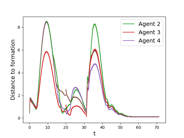
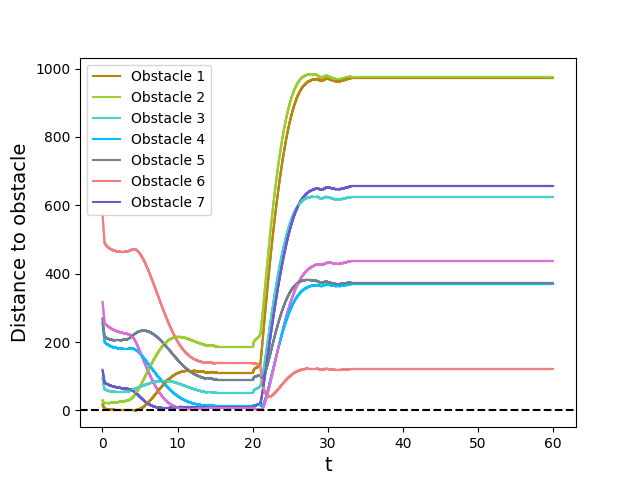
Figure 3: Evolution in the first simulation environment, cf. Figure 2. (left): Distance to the desired formation position over time for the different followers. All followers asymptotically converge to their desired formation positions. (right): Distance to the different obstacles over time for the leader.

The second simulation is in an environment with eight different rooms. Initially, a team of three Husky robots is located in one of the rooms, cf. Figure 4(left). The team traverses the environment while maintaining a triangular formation by following the leader (the robot tracing a green trajectory). The leader follows three waypoints consecutively as seen in Figure 4(right). Collision avoidance with the walls is achieved by approximating them with a set of ellipsoidal barrier functions. The team successfully completes the task by avoiding collision with the walls and between the robots, and reaching all waypoints while maintaining the desired formation.

Figure 4: Snapshots of the second simulation environment with color coded trajectories for the different robots. The intensity of the color increases with time. In the last snapshot, the red x’s indicate the four different waypoints for the leader of the team. The environment has dimensions $20$m $\times$ $50$m.

We have also validated our distributed control design in hardware in a team of 3 Jackal robots, which are small, entry-level research-focused robots with fully integrated GPS, IMU, and LIDAR sensors. The team is initially positioned as shown in Figure 5(left). The blue and grey cilinders are modelled as obstacles using CBFs. The team traverses the environment while maintaining a triangular formation by following the leader (the robot tracing the green trajectory). The leader follows two waypoints consecutively as seen in Figure 5(right). All computations are done onboard with the computers of each of the robots. Similarly as in the simulation experiments, the robots’ LIDAR sensors are used to run a SLAM system that allows each robot to localize itself in the environment and obtain its current state.

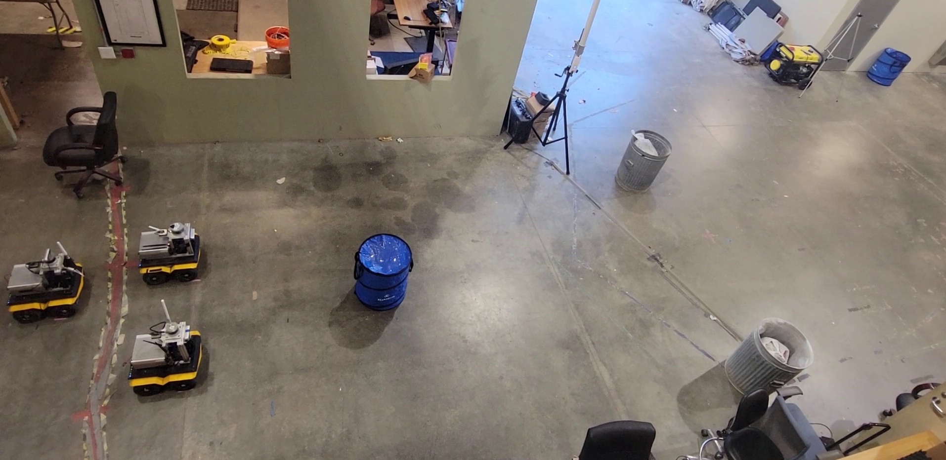
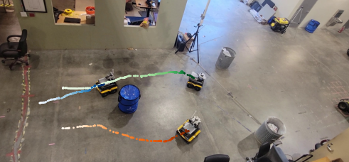
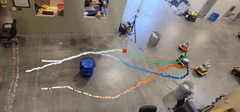
Figure 5: Snapshots of the hardware experiment with color coded trajectories for the different robots. The intensity of the color increases with time. In the last snapshot, the red x’s indicate the two different waypoints for the leader of the team. The environment has dimensions $4$m $\times$ $50$m.

VII Conclusions

We have proposed a distributed controller design based on the algorithmic solution of state-dependent network optimization algorithms with coupling constraints. When interconnected with the network dynamics, our controller is guaranteed to be asymptotically optimal and satisfy the constraints of the optimization problem at all times. We have leveraged the proposed framework to provide a distributed solution that achieves safe navigation for a team of differential-drive robots in environments with obstacles, avoiding collisions and maintaining a desired formation, using control barrier functions. We have illustrated its performance both in simulation and with real robots. Future work will design sequences of waypoints that ensure the network optimization problem remains feasible at all times, investigate heuristics to tune the parameters of our controller for improved performance, and explore the extension to settings with partial knowledge of the environment and the obstacles.

The regularized version of (17) takes the following form:

$$\min\limits_{u\in^{mN},z\in^{q}}\sum_{i=1}^{N}f_{i}(\xi_{i},u_{i})+\epsilon\sum_{k=1}^{p}\sum_{j\in V(\mathcal{G}_{k})}(z_{j}^{k})^{2},$$ (23)

$$\text{s.t.}\quad g_{i}^{k}(\xi_{\mathcal{N}_{i}},u_{i})+\!\!\!\!\!\!\!\sum_{j\in\mathcal{N}_{i}\cap V(\mathcal{G}_{k})}\!\!\!\!(z_{i}^{k}\!-\!z_{j}^{k})\leq 0,\ i\!\in\!V(\mathcal{G}_{k}),\ k\!\in\![p].$$

The next sensitivity result shows that the solution to (23) and (17) can be made close.

Lemma .1

(Sensitivity of regularized problem): Let $u^{*}$ be continuous, and assume $u^{*,\epsilon}$ is continuous for all $\epsilon>0$. Let $\mathcal{K}\subset^{nN}$ be a compact set and $\delta>0$. Then, there exists $\bar{\epsilon}_{\mathcal{K},\delta}>0$ such that if $\epsilon<\bar{\epsilon}_{\mathcal{K},\delta}$, then $\lVert u^{*,\epsilon}(\xi)-u^{*}(\xi)\rVert\leq\delta$ for all $\xi\in\mathcal{K}$.

Proof:

By [17, Lemma 4.2], for each $\xi\in\mathcal{K}$, there exists $\bar{\epsilon}_{\xi,\delta}>0$ such that if $\epsilon<\bar{\epsilon}_{\xi,\delta}$, then $\lVert u^{*,\epsilon}(\xi)-u^{*}(\xi)\rVert\leq\frac{\delta}{2}$. Now, since $u^{*,\epsilon}$ and $u^{*}$ are continuous, there exists a neighborhood $\mathcal{N}_{\xi}$ of $\xi$ such that $\lVert u^{*,\epsilon}(\hat{\xi})-u^{*}(\hat{\xi})\rVert\leq\delta$ for all $\hat{\xi}\in\mathcal{N}_{\xi}$. Since $\cup_{\xi\in\mathcal{K}}\mathcal{N}_{\xi}$ is an open covering of the compact set $\mathcal{K}$, there exists a finite subcover, i.e., there exists $N_{\mathcal{K}}\in\mathbb{Z}_{>0}$ and $\xi_{1},\xi_{2},\ldots,\xi_{N_{\mathcal{K}}}$ such that $\mathcal{K}\subset\cup_{i=1}^{N_{\mathcal{K}}}\mathcal{N}_{\xi_{i}}$. The result follows by letting $\bar{\epsilon}_{\mathcal{K},\delta}:=\min\{\bar{\epsilon}_{\xi_{1},\delta},\ldots,\bar{\epsilon}_{\xi_{N_{\mathcal{K}}},\delta}\}$. ∎

Lemma .1 ensures that in all of the results in Section IV, one can assume a fixed value of $\epsilon$ has been chosen sufficiently small to guarantee a desired maximum distance between the optimizers of the regularized and unregularized problems in a compact set of interest.

References

- [1] A. D. Ames, S. Coogan, M. Egerstedt, G. Notomista, K. Sreenath, and P. Tabuada, “Control barrier functions: theory and applications,” in European Control Conference, Naples, Italy, 2019, pp. 3420–3431.
- [2] P. Wieland and F. Allgöwer, “Constructive safety using control barrier functions,” IFAC Proceedings Volumes, vol. 40, no. 12, pp. 462–467, 2007.
- [3] A. D. Ames, X. Xu, J. W. Grizzle, and P. Tabuada, “Control barrier function based quadratic programs for safety critical systems,” IEEE Transactions on Automatic Control, vol. 62, no. 8, pp. 3861–3876, 2017.
- [4] A. Hauswirth, S. Bolognani, G. Hug, and F. Dörfler, “Optimization algorithms as robust feedback controllers,” arXiv preprint arXiv:2103.11329, 2021.
- [5] M. Colombino, E. Dall’Anese, and A. Bernstein, “Online optimization as a feedback controller: Stability and tracking,” IEEE Transactions on Control of Network Systems, vol. 7, no. 1, pp. 422–432, 2020.
- [6] B. J. Morris, M. J. Powell, and A. D. Ames, “Continuity and smoothness properties of nonlinear optimization-based feedback controllers,” in IEEE Conf. on Decision and Control, Osaka, Japan, Dec 2015, pp. 151–158.
- [7] P. Mestres, A. Allibhoy, and J. Cortés, “Robinson’s counterexample and regularity properties of optimization-based controllers,” Systems & Control Letters, 2023, submitted. Available at https://arxiv.org/abs/2311.13167.
- [8] R. W. Brockett, “Dynamical systems that sort lists, diagonalize matrices, and solve linear programming problems,” Linear Algebra and Its Applications, vol. 146, pp. 79–91, 1991.
- [9] U. Helmke and J. B. Moore, Optimization and Dynamical Systems. Springer, 1994.
- [10] M. Colombino, J. W. Simpson-Porco, and A. Bernstein, “Towards robustness guarantees for feedback-based optimization,” IEEE Conf. on Decision and Control, pp. 6207–6214, 2019.
- [11] A. Allibhoy and J. Cortés, “Control barrier function-based design of gradient flows for constrained nonlinear programming,” IEEE Transactions on Automatic Control, vol. 69, no. 6, 2024, to appear.
- [12] A. Colot, Y. Chen, B. Cornélusse, J. Cortés, and E. Dall’Anese, “Optimal power flow pursuit via feedback-based safe gradient flow,” IEEE Transactions on Smart Grid, 2024, submitted.
- [13] U. Borrmann, L. Wang, A. D. Ames, and M. Egerstedt, “Control barrier certificates for safe swarm behavior,” IFAC-PapersOnLine, vol. 48, no. 27, pp. 68–73, 2015.
- [14] L. Wang, A. Ames, and M. Egerstedt, “Safety barrier certificates for collisions-free multirobot systems,” IEEE Transactions on Robotics, vol. 33, no. 3, pp. 661–674, 2017.
- [15] M. Jankovic and M. Santillo, “Collision avoidance and liveness of multi-agent systems with CBF-based controllers,” in IEEE Conf. on Decision and Control, Austin, TX, USA, 2021, pp. 6822–6828.
- [16] X. Tan and D. V. Dimarogonas, “Distributed implementation of control barrier functions for multi-agent systems,” IEEE Control Systems Letters, vol. 6, pp. 1879–1884, 2022.
- [17] P. Mestres and J. Cortés, “Distributed and anytime algorithm for network optimization problems with separable structure,” in IEEE Conf. on Decision and Control, Singapore, 2023, pp. 5457–5462.
- [18] A. Cherukuri, E. Mallada, S. H. Low, and J. Cortés, “The role of convexity in saddle-point dynamics: Lyapunov function and robustness,” IEEE Transactions on Automatic Control, vol. 63, no. 8, pp. 2449–2464, 2018.
- [19] A. Cherukuri and J. Cortés, “Distributed algorithms for convex network optimization under non-sparse equality constraints,” in Allerton Conf. on Communications, Control and Computing, Monticello, IL, Sep. 2016, pp. 452–459.
- [20] P. Glotfelter, I. Buckley, and M. Egerstedt, “Hybrid nonsmooth barrier functions with applications to provably safe and composable collision avoidance for robotic systems,” IEEE Robotics and Automation Letters, vol. 4, no. 2, pp. 1303–1310, 2019.
- [21] M. Aicardi, G. Casalino, A. Bicchi, and A. Balestrino, “Closed Loop Steering of Unicycle-like Vehicles via Lyapunov Techniques,” IEEE Robotics and Automation Magazine, vol. 2, no. 1, pp. 27–35, 1995.
- [22] P. Mestres and J. Cortés, “Optimization-based safe stabilizing feedback with guaranteed region of attraction,” IEEE Control Systems Letters, vol. 7, pp. 367–372, 2023.
- [23] X. Xu, “Constrained control of input-output linearizable systems using control sharing barrier functions,” Automatica, vol. 87, pp. 195–201, 2018.
- [24] B. Stellato, G. Banjac, P. Goulart, A. Bemporad, and S. Boyd, “OSQP: an operator splitting solver for quadratic programs,” Mathematical Programming Computation, vol. 12, pp. 637–672, 2020.
- [25] X. Tan and D. V. Dimarogonas, “On the undesired equilibria induced by control barrier function based quadratic programs,” Automatica, vol. 159, p. 111359, 2013.
- [26] J. Liu, “Sensitivity analysis in nonlinear programs and variational inequalities via continuous selections,” SIAM Journal on Control and Optimization, vol. 33, no. 4, pp. 1040–1060, 1995.
- [27] S. M. Robinson, “Strongly regular generalized equations,” Mathematics of Operations Research, vol. 5, no. 1, pp. 43–62, 1980.
- [28] H. Khalil, Nonlinear Systems, 3rd ed. Englewood Cliffs, NJ: Prentice Hall, 2002.
- [29] F. Watbled, “On singular perturbations for differential inclusions on the infinite interval,” Journal of Mathematical Analysis and Applications, vol. 310, no. 2, pp. 362–378, 2005.
- [30] W. S. Cortez and D. V. Dimarogonas, “On compatibility and region of attraction for safe, stabilizing control laws,” IEEE Transactions on Automatic Control, vol. 67, no. 9, pp. 7706–7712, 2022.
- [31] M. F. Reis, A. P. Aguilar, and P. Tabuada, “Control barrier function-based quadratic programs introduce undesirable asymptotically stable equilibria,” IEEE Control Systems Letters, vol. 5, no. 2, pp. 731–736, 2021.
- [32] P. Virtanen, R. Gommers, T. E. Oliphant et al., “SciPy 1.0: Fundamental Algorithms for Scientific Computing in Python,” Nature Methods, vol. 17, pp. 261–272, 2020.
- [33] M. S. Andersen, J. Dahl, and L. Vandenberghe, “CVXOPT: A python package for convex optimization, version 1.1.6.” Available at cvxopt.org, 2013, 2013.