SMC Is All You Need: Parallel Strong Scaling

Abstract

In the general framework of Bayesian inference, the target distribution can only be evaluated up-to a constant of proportionality. Classical consistent Bayesian methods such as sequential Monte Carlo (SMC) and Markov chain Monte Carlo (MCMC) have unbounded time complexity requirements. We develop a fully parallel sequential Monte Carlo (pSMC) method which provably delivers parallel strong scaling, i.e. the time complexity (and per-node memory) remains bounded if the number of asynchronous processes is allowed to grow. More precisely, the pSMC has a theoretical convergence rate of MSE$=O(1/NR)$, where $N$ denotes the number of communicating samples in each processor and $R$ denotes the number of processors. In particular, for suitably-large problem-dependent $N$, as $R\rightarrow\infty$ the method converges to infinitesimal accuracy MSE$=O(\varepsilon^{2})$ with a fixed finite time-complexity Cost$=O(1)$ and with no efficiency leakage, i.e. computational complexity Cost$=O(\varepsilon^{-2})$. A number of Bayesian inference problems are taken into consideration to compare the pSMC and MCMC methods.

1 Introduction

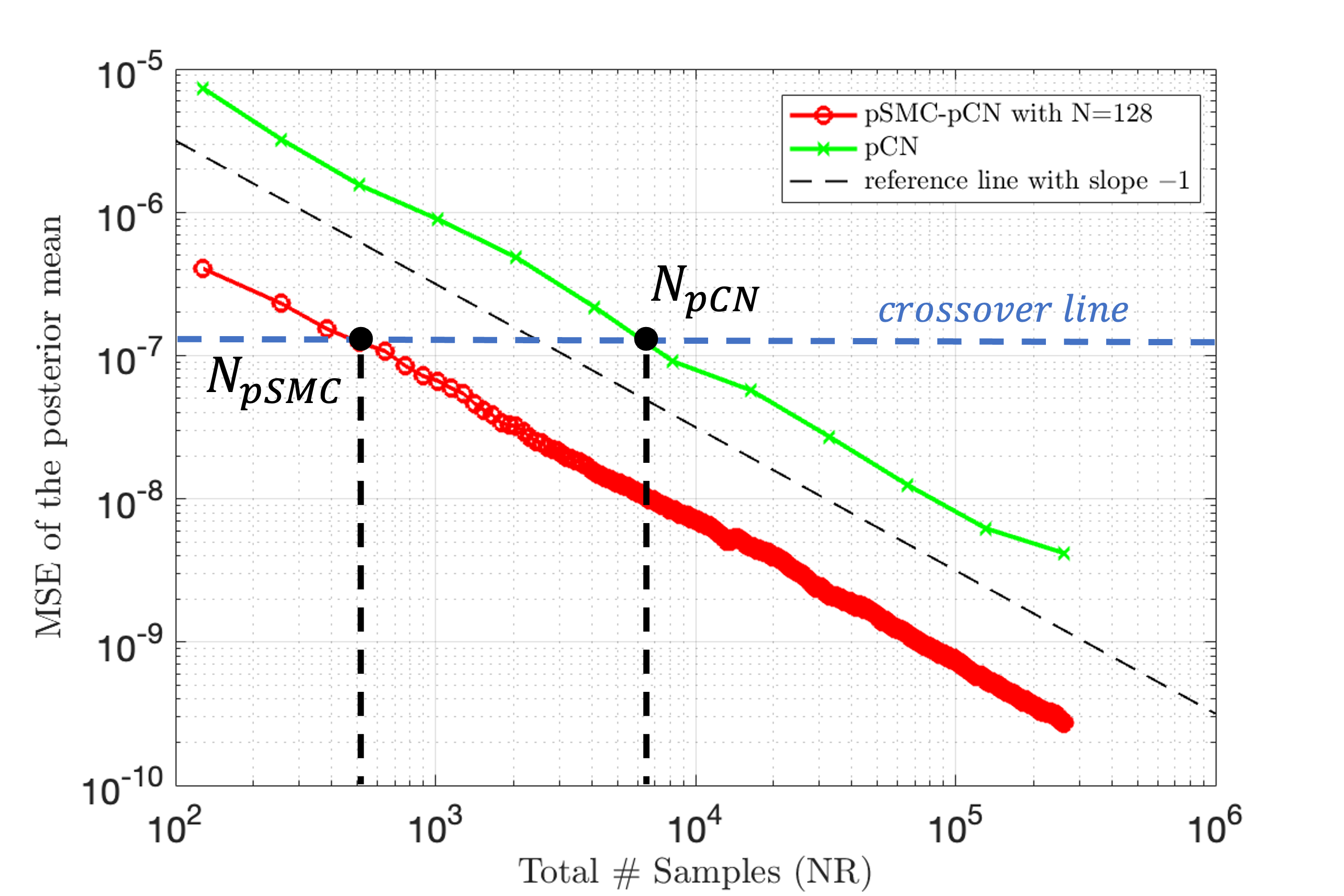
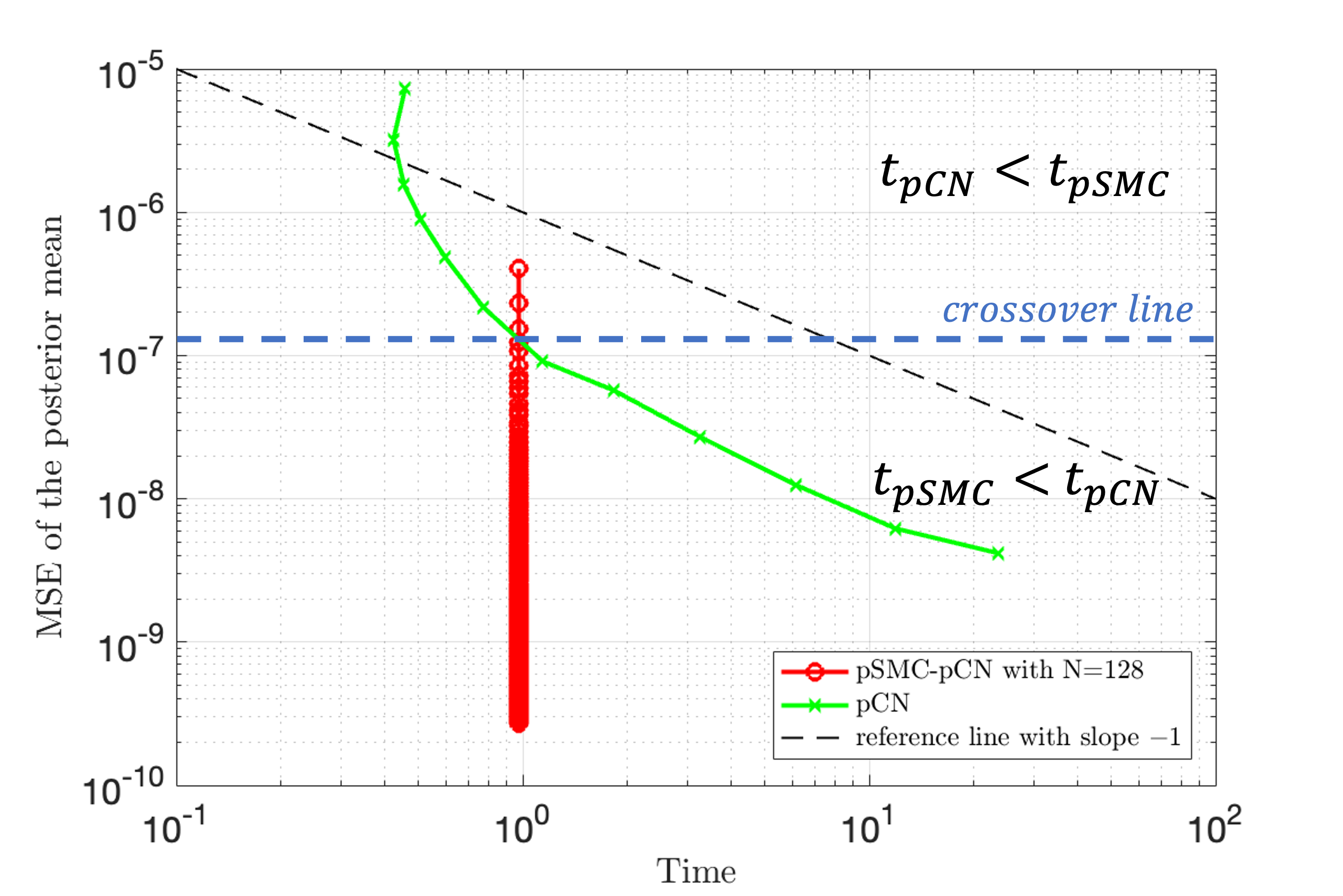
Figure 1: Convergence of the MCMC method pCN, and our pSMC method with pCN kernel. The crossover line separates the pSMC-preferred regime with the pCN-preferred regime. The example is a Gaussian Bayesian linear model with $m\times d=16\times 4$ dimensional design matrix. See Section 4.1 for further details.

The Bayesian paradigm for machine learning can be traced back at least to the 1990s [MacKay, 1992, Neal, 1993, Hinton et al., 1986, Ng and Jordan, 1999, Bengio, 2000, Andrieu et al., 2003, Bishop, 2006, Murphy, 2012]. It is attractive because it delivers the Bayes estimator, along with principled quantification of uncertainty. However, in general the posterior (target) distribution can only be evaluated up-to a constant of proportionality, and the only consistent methods available for inference are of Monte Carlo type: notably Markov chain Monte Carlo (MCMC) and sequential Monte Carlo (SMC). These are still too expensive to be used in practice for anything except ground truth approximation for toy problems, and variational Bayesian approximation methods have taken centre stage in the context of Bayesian deep learning [Blundell et al., 2015, Gal and Ghahramani, 2016]. The present work addresses the computational intractability head-on by proposing a method which can distribute the workload across arbitrarily many workers. As such, the aim is to revive interest in Bayesian MC methods as both optimal and practical.

Given data $\mathcal{D}$, the Bayesian posterior distribution over $\theta\in\mathsf{\Theta}\in\mathbb{R}^{d}$ is given by:

$$\pi(\theta)\propto\mathcal{L}(\theta)\pi_{0}(\theta),$$ (1)

where $\mathcal{L}(\theta):=\mathcal{L}(\mathcal{D}|\theta)$ is the likelihood for the given data $\mathcal{D}$ and $\pi_{0}(\theta)$ is the prior. The Bayes estimator of a quantity of interest $\varphi:\mathsf{\Theta}\rightarrow\mathbb{R}$ is $\int_{\mathsf{\Theta}}\varphi(\theta)\pi(\theta)d\theta$. It minimizes the appropriate frequentist risk at the population level and can therefore be considered optimal.

Markov chain Monte Carlo methods (MCMC) originated with the famous Metropolis-Hastings (MH) methods [Metropolis et al., 1953, Hastings, 1970], and are the favoured approach to consistently approximate this kind of target distribution in general. MCMC has seen widespread use and rigorous development in statistics from the turn of the millennium [Gelfand and Smith, 1990, Geyer, 1992, Robert et al., 1999, Roberts and Tweedie, 1996, Duane et al., 1987]. One crowning achievement is overcoming the so-called “curse-of-dimensionality”, i.e. exponential degradation, in the rate of convergence. Nonetheless, some dimension-dependence typically remains in the constant for the aforementioned MCMC methods. It was recently shown that the performance of a carefully constructed MH kernel [Neal, 1998] can be completely dimension-independent [Cotter et al., 2013]. We adopt the name precondition Crank-Nicholson (pCN) method, introduced in the latter. Shortly thereafter, the convergence properties of vanilla pCN were further improved by leveraging Hessian and/or covariance information in the transition kernel [Law, 2014, Cui et al., 2016, Rudolf and Sprungk, 2018, Beskos et al., 2017]. The Hamiltonian Monte Carlo (HMC) method Duane et al. [1987], Neal [1993], Houlsby et al. [2011] is a hybrid method which interleaves Metropolis-Hastings type accept/reject with evolution in an extended phase-space to circumvent random walk behaviour and enable better mixing. This is perhaps the most popular MCMC method in use in the machine learning community. Despite its attractive properties, MCMC is much more expensive to use in practice in comparison to point-estimators or variational methods and is still in minority use. There has been some effort in parallelizing MCMC [Chen et al., 2016], with the most elegant and widely-recognized work being Jacob et al. [2020]. Nonetheless, these methods lack theory and/or are awkward and cumbersome to implement in practice, and have not caught on.

The sequential Monte Carlo (SMC) sampler [Del Moral et al., 2006] is an alternative population-based method which developed at the turn of the millennium Jarzynski [1997], Berzuini and Gilks [2001], Gilks and Berzuini [2001], Neal [2001], Chopin [2002]. The SMC sampler approximates the target distribution $\pi$ through a sequence of tempering distributions $\pi_{j}$, starting from a simulable distribution such as the prior $\pi_{0}$. A population of sample “particles” from $\pi_{0}$ evolve through importance re-sampling (selection) and MCMC moves (mutation) between successive tempering distributions. See the following for recent thorough introductions Dai et al. [2022], Chopin et al. [2020]. SMC gracefully handles multi-modality and facilitates adaptive tuning of the Markov kernel, with only a small theoretical efficiency overhead with respect to MCMC. It also delivers an unbiased estimator of the normalizing constant, or model evidence, which can be useful in practice. Furthermore, the structure of SMC method facilitates parallelisation at multiple levels.

The parallel implementation of the SMC method has already been considered in Vergé et al. [2015], Whiteley et al. [2015], however the existing methods involve communication between all samples, which hinders implementation. The island particle model [Vergé et al., 2015] separates the total number of sample $NR$ into $R$ islands and each island has $N$ samples. Two levels of resampling is needed in each tempering step: first, particles within each island are selected by resampling separately, and then islands themselves undergo selection by resampling at the island level. The method guarantees the MSE$=O(1/NR)$ convergence rate, but requires (frequent) communication between all samples, thereby undermining the parallelism in a sense: all processes have to wait for the slowest one and the method is exposed to I/O bottlenecks at every sync point. Without these interactions, the island particle method has a penalty of $1/N^{2}$, and as $R\gg N$, the penalty becomes noticeable.

The present work introduces the parallel SMC (pSMC) sampler, which can be viewed as a judicious estimator built from an island particle filter without any interaction between islands. We provide a simple proof that our estimator converges with the rate MSE$=O(1/NR)$, and without the $1/N^{2}$ bias, under reasonable and mild assumptions. In particular, the estimator delivers parallel strong scaling, in the sense that for any given problem it converges for fixed (suitably large) $N$ as $R\rightarrow\infty$, and without any loss of efficiency: with $R$ non-interacting processors, the method converges at the rate $MSE=O(1/R)$ with $O(1)$ time complexity. It has come to our attention after writing this that the very general $\alpha$SMC method [Whiteley et al., 2015] actually includes a very similar method as a special case, hence also overcoming the interaction limitation and bias of the island particle filter, however it is mentioned only parenthetically and not simulated or investigated thoroughly. That work is focused instead on achieving stability for online SMC algorithms, on the infinite time horizon, in exchange for allowing communication between all samples.

The paper is organized as follows. In Section 2, we restate the algorithm for a single SMC and provide a summary of various MCMC kernels. In Section 3, the general framework of pSMC is established. In Section 3.1, the theoretical results for the convergence of pSMC are given. In Section 4, a number of Bayesian inference problems, including the Gaussian, trace-class neural network, and quantum state tomography problems, are examined in order to compare the pSMC and pCN. In Section 5, the conclusion and additional discussion are addressed.

2 SMC sampler

Define the target distribution as $\pi(\theta)=f(\theta)/Z$, where $Z=\int_{\mathsf{\Theta}}f(\theta)d\theta$ and $f(\theta):=\mathcal{L}(\theta)\pi_{0}(\theta)$. Given a quantity of interest $\varphi:\mathsf{\Theta}\rightarrow\mathbb{R}$, for simplicity, we define

$$f(\varphi):=\int_{\mathsf{\Theta}}\varphi(\theta)f(\theta)d\theta=f(1)\pi(\varphi),$$

where $f(1)=\int_{\mathsf{\Theta}}f(\theta)d\theta=Z$.

So, the target expectation can be computed by

$$\pi(\varphi)=\frac{f(\varphi)}{f(1)}.$$

Define $h_{1},...,h_{J-1}$ by $h_{j}=f_{j+1}/f_{j}$, where $f_{1}=\pi_{0},f_{J}=f=\mathcal{L}(\theta)\pi_{0}(\theta)$, and define $\pi_{j}=f_{j}/Z_{j}$ where $Z_{j}=\int_{\mathsf{\Theta}}f_{j}d\theta$. For $j=2,...,J$, we let $f_{j}$ define in a annealing scheme:

$$f_{j}=f_{1}^{1-\lambda_{j}}f_{J}^{\lambda_{j}}=\mathcal{L}(\theta)^{\lambda_{j}}\pi_{0}(\theta),$$

where $0=\lambda_{1}<\lambda_{2}<\cdots<\lambda_{J}=1$ and $\lambda_{j}$ will be chosen adaptively according to the effective sample size (ESS), see Example 2.1.

Example 2.1 (Adaptive tempering).

In order to keep the sufficient diversity of sample population, we let the effective sample size to be at least $ESS_{\min}=N/2$ at each tempering $\lambda_{j-1}$ and use it compute the next tempering $\lambda_{j}$. For $j$th tempering, we have weight samples $\{w^{k}_{j-1},\theta^{k}_{j-1}\}_{k=1}^{N}$, then the ESS is computed by

$$ESS=\frac{1}{\sum_{k=1}^{N}(w^{k}_{j-1})^{2}},$$

where $w^{k}_{j-1}=\mathcal{L}(\theta^{k}_{j-1})^{\lambda_{j}-\lambda_{j-1}}/\sum_{k=1}^{N}\mathcal{L}(\theta_{j-1}^{k})^{\lambda_{j}-\lambda_{j-1}}$. Let $h=\lambda_{j}-\lambda_{j-1}$, the effective sample size can be presented as a function of $h$, ESS$(h)$. Using suitable root finding method, one can find $h^{*}$ such that $ESS(h^{*})=ESS_{\min}$, then set the next tempering $\lambda_{j}=\lambda_{j-1}+h^{*}$.

Now let $\mathcal{M}_{j}$ for $j=2,\dots,J$ be Markov transition kernels such that $(\pi_{j}\mathcal{M}_{j})(d\theta)=\pi_{j}(d\theta)$, analogous to any suitable MCMC kernel [Geyer, 1992, Robert et al., 1999, Cotter et al., 2013, Law, 2014]. This operation must sufficiently decorrelate the samples, and as such we typically define the MCMC kernels ${\mathcal{M}_{j}}$ by $M$ steps of some basic MCMC kernel, where $M$ may or may not be 1. We call $M$ the mutation parameter.

Algorithm 1 SMC sampler

  Generate $\theta^{i}_{1}\sim\pi_{1}$ for $i=1,...,N$ and $Z^{N}_{1}=1$.

  for $j=2$ to $J$ do

     Store $Z^{N}_{j}=Z^{N}_{j-1}\frac{1}{N}\sum_{k=1}^{N}\mathcal{L}(\theta_{j-1}^{k})^{\lambda_{j}-\lambda_{j-1}}$.

     for $i=1$ to $N$ do

        Define $w^{i}_{j}=\mathcal{L}(\theta_{j-1}^{k})^{\lambda_{j}-\lambda_{j-1}}/\sum_{k=1}^{N}\mathcal{L}(\theta_{j-1}^{k})^{\lambda_{j}-\lambda_{j-1}}$.

        Resample: Select $I_{j}^{i}\sim\{w_{j}^{1},...,w_{j}^{N}\}$ and let $\hat{\theta}_{j}^{i}=\theta_{j-1}^{I_{j}^{i}}$.

        Mutate: Draw $\theta_{j}^{i}\sim\mathcal{M}_{j}(\hat{\theta}_{j}^{i},\cdot)$.

     end for

  end for

One can observe that

$$\pi_{j}(h_{j})=\frac{1}{Z_{j}}\int\frac{f_{j+1}(\theta)}{f_{j}(\theta)}f_{j}(\theta)d\theta=\frac{Z_{j+1}}{Z_{j}}.$$

Since we let $\pi_{J}=\pi$ be the target distribution and $Z_{1}=1$, the normalisation constant of $\pi$ is given by

$$Z_{J}=Z_{1}\prod_{j=1}^{J-1}\pi_{j}(h_{j})=\prod_{j=1}^{J-1}\pi_{j}(h_{j}).$$

From Algorithm 1, we can define the following estimators:

$$\pi_{j}^{N}(h_{j}) :=\frac{1}{N}\sum_{i=1}^{N}h_{j}(\theta_{j}^{i}),\ i=1,...,J,$$ (2)

$$Z_{J}^{N} :=\prod_{j=1}^{J-1}\pi_{j}^{N}(h_{j}),$$

$$f_{J}^{N}(\varphi) :=\prod_{j=1}^{J-1}\pi_{j}^{N}(h_{j})\pi_{J}^{N}(\varphi)=Z_{J}^{N}\pi_{J}^{N}(\varphi).$$

Hence, the sequential Monte Carlo estimator for estimating the expectation of the quantity of interest is given by

$$\hat{\varphi}_{\text{SMC}}=\pi^{N}(\varphi)=\pi_{J}^{N}(\varphi)=\frac{f_{J}^{N}(\varphi)}{Z_{J}^{N}}=\frac{f^{N}(\varphi)}{f^{N}(1)}.$$ (3)

The SMC sampler can employ and potentially accelerate any appropriate MCMC approach. Here, the following MCMC kernels are introduced.

2.1 Pre-conditioned Crank-Nicolson kernel

By slightly changing the random walk MH kernel, one can ensure stability of the proposal chain and stationarity with respect to a specified Gaussian distribution. For posteriors with Gaussian priors, including for Gaussian measures over infinite-dimensional function spaces this leads to a stable MH method which depends only on the properties of the likelihood. For a prior $N(\mu_{0},\Sigma_{0})$, the pCN proposal is

$$\theta^{\prime}=(a-\beta^{2})^{1/2}(\theta-\mu_{0})+\mu_{0}+\Sigma_{0}^{1/2}\delta\,,\qquad\delta\sim N(0,I_{d})\,.$$

See Neal [1998], Cotter et al. [2013] for further details.

An enhancement for the pCN kernel involves employing the operator-weighted proposal [Law, 2014, Cui et al., 2016], which employs the covariance matrix of the current state within the mutation kernel rather than the identity matrix, thus improving mixing when the likelihood informs certain directions much more than others. The general pCN kernel is given by

$$\theta^{\prime}=\Sigma_{0}^{1/2}(I_{d}-\beta^{2}D)^{1/2}\Sigma_{0}^{-1/2}(\theta-\mu_{0})+\mu_{0}+\Sigma_{0}^{1/2}\beta D^{1/2}\delta\,.$$

The scaling matrix $D$ should be chosen according to the information present in the likelihood. A simple and computationally convenient choice which is particularly amenable to use within SMC is to build it from an approximation of the target covariance [Beskos et al., 2018]. In the present work we adopt the simplest and cheapest choice and let $D=\text{diag}(\widehat{\text{var}}[\theta])$. The approximation of the variance, $\widehat{\text{var}}$, will be built from the current population of samples in the SMC case, and adaptively constructed in the MCMC case [Haario et al., 2001, Chen et al., 2016]. See also [Rudolf and Sprungk, 2018, Beskos, 2014, Zahm et al., 2022].

Algorithm 2 pCN kernel

  Give a current state $\theta$, the distribution $\pi_{j}$, a scaling parameter $\beta$.

  for $m=1$ to $M$ do

     Generate $\theta^{\prime}=\Sigma_{0}^{1/2}(I_{d}-\beta^{2}D)^{1/2}\Sigma_{0}^{-1/2}(\theta-\mu_{0})+\mu_{0}+\Sigma_{0}^{1/2}\beta D^{1/2}\delta$ where $\delta\sim N(0,I_{d})$ and $u\sim U([0,1])$.

     if $u\leq\min\Big{\{}1,\frac{\mathcal{L}(\theta^{\prime})^{\lambda_{j}}}{\mathcal{L}(\theta)^{\lambda_{j}}}\Big{\}}$ then

        $\theta=\theta^{\prime}$.

     else

        $\theta=\theta$.

     end if

  end for

2.2 Hamiltonian Monte Carlo

Algorithm 3 Hamiltonian Monte Carlo kernel

  Give a current state $\theta$, the distribution $\pi_{j}$ and a mass matrix $M_{0}$.

  Generate a initial momentum $p\sim N(0,M_{0})$.

  for $m=1$ to $M$ do

     for $l=1$ to $L$ do

        Generate $\theta_{l\Delta t}$ and $p_{l\Delta t}$ from (LABEL:eqn:leapfrog_step) with $\theta_{0}=\theta$ and $p_{0}=p$

     end for

     Let $\theta^{\prime}=\theta_{L\Delta t}$ and generate $u\sim U([0,1])$

     if $u\leq\min\Big{\{}1,\frac{H(\theta^{\prime},p^{\prime})}{H(\theta,p)}\Big{\}}$ then

        $\theta=\theta^{\prime}$ and $p=p^{\prime}$.

     else

        $\theta=\theta$ and $p=p$.

     end if

  end for

Hamiltonian Monte Carlo (HMC) kernel [Duane et al., 1987, Neal et al., 2011, Houlsby et al., 2011, Cobb and Jalaian, 2021] is essentially a gradient-based MCMC kernel on an extended state-space. We first build a Hamiltonian $H(\theta,p)$ with additional auxiliary “momentum” vector $p$ of the same dimension as the state $\theta$

$$H(\theta,p)=-\log\pi_{j}(\theta)+\frac{1}{2}p^{\top}M_{0}^{-1}p,$$ (4)

where $M_{0}$ is a mass matrix, so that $\frac{1}{Z}\exp(H(\theta,p))$ is a target distribution on the extended space, where the momentum can be simulated exactly $p\sim N(0,M_{0})$.

From physics we know that the Hamiltonian dynamics conserve energy, hence avoiding local random-walk type behaviour and allowing ballistic moves in position:

$$\frac{d\theta}{dt}=\frac{\partial H}{\partial p}=M_{0}^{-1}p,$$ (5)

$$\frac{dp}{dt}=\frac{\partial H}{\partial\theta}=\nabla_{\theta}\log\pi_{j}(\theta)\,.$$

A carefully constructed symplectic-integrator is capable of conserving energy as well, for example the leapfrog integrator Leimkuhler and Reich [2004]:

$$p_{t+\Delta t/2}=p_{t}+\frac{\Delta t}{2}\frac{dp}{dt}(\theta_{t}),$$ (6)

$$\theta_{t+\Delta t}=\theta_{t}+\Delta t\frac{d\theta}{dt}(p_{t+\Delta t/2}),$$

$$p_{t+\Delta t}=p_{t+\Delta t/2}+\frac{\Delta t}{2}\frac{dp}{dt}(\theta_{t+\Delta t}),$$

where $t$ is the leapfrog step iteration and $\Delta t$ is the step size.

Each step of the HMC method is summarized as follows:

• simulate a random momentum $p\sim N(0,M_{0})$ (hence jumping to a new energy contour);

• approximate the Hamiltonian dynamics using $L$ steps from (LABEL:eqn:leapfrog_step);

• correct numerical error from (ii) with an MH accept/reject step for $\frac{1}{Z}\exp(H(\theta,p))$.

See Algorithm 3.

3 Parallel SMC method

By separating $NR$ samples into $R$ processors with $N$ samples in each, the parallel SMC sampler has a $R$ times lower time complexity than a single SMC sampler. This reduction in time complexity is crucial if we encounter an expensive SMC, which is common in the high-dimensional Bayesian inference problem. More importantly, under reasonable and mild assumptions we will demonstrate the strong scaling property for pSMC: the cost decreases linearly with the number of cores with constant time. The Algorithm 4 displays the parallel SMC method.

Algorithm 4 Parallel SMC sampler

  for $r=1$ to $R$ do

     Run Algorithm 1, output $\theta^{N,r}$.

     Compute the estimators $Z^{N,r}$, $f^{N,r}(\varphi)$, $f^{N,r}(1)$ and $\pi^{N,r}(\varphi)$ by (2).

  end for

Following from Algorithm 4, we can define the unnormalized estimators

$$F^{N,R}(\varphi) =\frac{1}{R}\sum_{r=1}^{R}f^{N,r}(\varphi),$$ (7)

$$F^{N,R}(1) =\frac{1}{R}\sum_{r=1}^{R}f^{N,r}(1)=\frac{1}{R}\sum_{r=1}^{R}Z^{N,r}.$$ (8)

Then, the parallel SMC estimator for estimating $\pi[\varphi]$ is given by

$$\hat{\varphi}_{\text{pSMC}}=\frac{F^{N,R}(\varphi)}{F^{N,R}(1)}=\frac{\sum_{r=1}^{R}f^{N,r}(\varphi)}{\sum_{r=1}^{R}f^{N,r}(1)}.$$ (9)

3.1 Theoretical results for parallel strong scaling

In order to make use of (9), we define $f^{N,r}(\zeta)$ both for quantity of interest $\zeta=\varphi$ and $\zeta=1$. We denote that $|\zeta|_{\infty}=\max_{\theta\in\mathsf{\Theta}}|\zeta(\theta)|$ in the following equations. $C_{\zeta}$ denotes the constant depended on the function $\zeta$. Note that using $\varphi$ with one-dimensional output is without loss of generality for our convergence results, and the following proof can be directly generalized to the multi-output function by using the inner product.

Assumption 3.1.

Let $J\in\mathbb{N}$ be given, for each $j\in\{1,...,J\}$, there exists a $C>0$ such that for all $\theta\in\mathsf{\Theta}$,

$$C^{-1}<\ f_{j}(\theta),\ \mathcal{L}(\theta)\leq C.$$

Assumption 3.2.

Let $J\in\mathbb{N}$ be given, for each $j\in\{1,...,J\}$, there exists a $\rho\in(0,1)$ such that for any $(u,v)\in\mathsf{\Theta}^{2}$, $A$ is a measureable set from the space containing all the measureable subset of $\mathsf{\Theta}$,

$$\int_{A}\mathcal{M}_{j}(u,du^{\prime})\geq\rho\int_{A}\mathcal{M}_{j}(v,dv^{\prime}).$$

First, we restate the convergence result for the non-parallelized SMC method in Proposition 3.3, which is from Del Moral [2004].

Proposition 3.3.

Assume Assumption 3.1 and 3.2. Then, for any $J\in\mathbb{N}$, there exists a $C>0$ such that for any $N\in\mathbb{N}$, suitable $\zeta:\mathsf{\Theta}\rightarrow\mathbb{R}$,

$$\mathbb{E}[(f^{N}(\zeta)-f(\zeta))^{2}]\leq\frac{C|\zeta|_{\infty}^{2}}{N}.$$ (10)

In addition, the estimator is unbiased $\mathbb{E}[f^{N}(\zeta)]=f(\zeta)$.

Lemma 3.4.

Assume Assumption 3.1 and 3.2. Then, for any $J\in\mathbb{N}$, there is a $C>0$ such that for any $N,R\in\mathbb{N}$, suitable $\zeta:\mathsf{\Theta}\rightarrow\mathbb{R}$,

$$\mathbb{E}[(F^{N,R}(\zeta)-f(\zeta))^{2}]\leq\frac{C|\zeta|_{\infty}^{2}}{NR}.$$

Theorem 3.5.

Assume Assumption 3.1 and 3.2. Then, for any $J\in\mathbb{N}$, there exists a $C_{\varphi}>0$, which depends on $\varphi$, such that for any $R\in\mathbb{N}$,

$$\mathbb{E}[(\hat{\varphi}_{\text{pSMC}}-\pi(\varphi))^{2}]\leq\frac{C_{\varphi}}{NR}.$$ (11)

Then the strong scaling in the parallel SMC is described as the MSE defined in (11) decreases as $1/R$ for $R$ nodes, for suitable variables value ($M$,$N$,$J$), with constant time.

3.2 Discussion of pSMC in practice

Table 1: Comparison between pCN and pSMC regarding to the time cost, memory cost and MSE.

	Time Cost	Memory Cost	MSE
pCN	COST$(d,m)NR$	$d(m+NR)$	$C_{\sf MCMC}^{2}(d,m)/NR$
pSMC	${\sf COST}(d,m){\sf COST}_{\sf over}(d,m)N$	$d(m+N)$	$C_{\sf SMC}^{2}(d,m)/NR$

Let $m$ denote the number of observations in the data. As Theorem 3.5 suggests, the nuisance parameters $(M,N,J)$ must be chosen large enough to ensure rapid convergence in $R$. For MCMC the error will be bounded by $C_{\sf MCMC}(d,m)/NR$, and the time (and total) cost will grow like ${\sf COST}(d,m)NR$, where ${\sf COST}$ is the basic cost of evaluating the likelihood (target) . Meanwhile, the error of SMC will be bounded by $C_{\sf SMC}(d,m)/N$, while the time cost will grow like ${\sf COST}(d,m)MJN$. Since $M$ and $J$ will also depend on $(d,m)$ – and need to be chosen larger for more complex targets – we will denote by ${\sf COST}_{\sf over}(d,m):=MJ$ the cost overhead of SMC vs MCMC for a given total number of samples.

Finally, we can achieve a fixed MSE of $\varepsilon^{2}$ with MCMC by selecting $NR=C_{\sf MCMC}(d,m)\varepsilon^{-2}$, which incurs a complexity of

$${\sf COST}(d,m)NR={\sf COST}(d,m)C_{\sf MCMC}(d,m)\varepsilon^{-2}\,.$$

Similarly, the time complexity of SMC will be

$${\sf COST}(d,m){\sf COST}_{\sf over}(d,m)N={\sf COST}(d,m){\sf COST}_{\sf over}(d,m)C_{\sf SMC}(d,m)\varepsilon^{-2}/R\,.$$

Equating these two, we can estimate the crossover

$$R>{\sf COST}_{\sf over}(d,m)C_{\sf SMC}(d,m)/C_{\sf MCMC}(d,m)\,.$$

For suitably chosen $M,J$, we expect $C_{\sf SMC}(d,m)\approx C_{\sf MCMC}(d,m)$, so the crossover should be roughly equivalent to ${\sf COST}_{\sf over}(d,m)$ processors.

The memory cost of $N$ samples of size $d$ is $Nd$, and the memory cost of storing the data is $O(dm)$. The latter may be considerably smaller, and even inconsequential, for neural network models with large number of parameters and smaller input dimension. Nonetheless, we take $O(d(m+N))$ as a proxy for the per process memory requirements of SMC. Meanwhile, if the quantity of interest is known a priori and estimated online, then MCMC samples do not need to be stored, resulting in a memory cost of only $O(dm)$. Of course, if one intends to perform inference in the future without saving samples, then the total memory cost is $O(d(m+NR))$, but the samples could be (thinned and) offloaded at checkpoints, so this can nevertheless be kept under control.

Clearly we require a minimum $N\gg C_{\sf SMC}(d,m)$ in order for the SMC theory to make sense, and we have indeed found that convergence slows or stops if this condition is not satisfied. This can be viewed as sufficient maximum population diversity. Furthermore, the samples must decorrelate sufficiently, leading to a minimum $M$, and they must be be rejuvenated sufficiently often, leading to a minimum $J$. Both of these conditions can also spoil convergence. Conventional advice suggests that it is safe to select $M=J=N=O(\max\{m,d\})$ Chopin et al. [2020]. If $d=m$, then the crossover occurs when $R>d^{2}$, and the memory requirement per processor is also $O(d^{2})$. In practice, we have found that the minimum required $M$ and $J$ often increase much slower than $O(d)$, so the crossover often occurs earlier than $d^{2}$.

Computing and storing the log-likelihood instead of the likelihood itself wherever possible in SMC sampler is preferred in practice to avoid numerical over/underflow. See Appendix A for further details.

4 Simulations

Table 2: The MSE, number of nodes for pSMC, and total time until the crossover point (see Figure 1) for the Gaussian examples, using pCN as the MCMC kernel.

	Gaussian m$\times$d = 64			Gaussian m$\times$d = 1024
	m=16 > d	m = 8 = d	m=4 < d	m = 64 > d	m = 32 = d	m = 16 < d
MSE	1.2332e-07	7.3838e-04	3.1846e+00	6.0035e-07	2.8125e-02	1.9128e+01
No.node	4	2	1	1	20	1
Time	0.9749	1.7513	1.7521	1.3517	6.0139	14.3041

Table 3: The MSE, number of nodes for pSMC, and total time until the crossover point (see Figure 1) for the non-Gaussian example of QST regression. For BNN classification, MSE is replaced with mean KL-divergence.

	QST (pCN)			BNN (HMC)
	(d,m) = (16,6)	(d,m) = (64,36)	(d,m) = (256,216)	iris (d,m) = (15,50)	MNIST (d,m) = (1177,50)
MSE/Loss	4.0111e-04	1.5068e-03	4.5424e-05	1.3936e-04	6.7747e-02
No.node	1	1	681	33	26
Time	0.0456	0.6681	29.6914	13.2356	34.5685

Applications of pSMC with different MCMC kernels on various Bayesian inference problems with/without analytical solutions are provided in this section. The notations pSMC-pCN and pSMC-HMC denote parallel SMC with pCN and HMC transition kernels, respectively.

4.1 High-dimensional Gaussian cases

Bayesian inference of Gaussian distributions are always tractable, in which the analytical solution of the posterior are solvable. Numerical verification of the convergence rate and strong scaling property of pSMC is provided by computing the MSE in relation to the analytical solution.

Consider a toy Gaussian inference example with $m$ observations ($y$) and $d$-dimensional parameter ($\theta$). Assume we have data $\mathcal{D}=\{y,X\}$, where $y\in\mathbb{R}^{m}$ and $X\in\mathbb{R}^{m\times d}$, and parameter $\theta\in\mathbb{R}^{d}$ connected by the following inverse problem:

$$y=X\theta+\nu,\ \nu\sim N(0,\sigma^{2}I_{m}),$$ (12)

where $X$ is the design matrix. If we let $\pi_{0}(\theta)=N(\mu_{0},\Sigma_{0})$, this is one of very few problems with an analytical Bayesian posterior, which will provide a convenient ground truth for measuring convergence. In particular, the posterior distribution is a multivariate Gaussian distribution $N(\mu,\Sigma)$, where

$$\mu=\Sigma(\Sigma_{0}^{-1}\mu_{0}+\frac{1}{\sigma^{2}}X^{T}y),\ \Sigma=(\Sigma_{0}^{-1}+\frac{1}{\sigma^{2}}X^{T}X)^{-1}.$$

See e.g. [Bishop, 2006].

In the following tests, we compare pSMC-pCN with pCN performance in estimation of the posterior mean, $\mu=\mathbb{E}[\theta|\mathcal{D}]$. Let $X\in\mathbb{R}^{m\times d}$ be a randomly selected full rank matrix and $\sigma=0.01$. The observations are generated as

$$y=X\theta^{*}+\nu,$$ (13)

where $\theta^{*}\sim\pi_{0}$ and $\nu\sim N(0,\sigma^{2}I_{m})$ are independent.

Three cases are examined: the over-observed case ($m\gg d$), the full-observed case ($m=d$) and the partial-observed case ($m\ll d$). If the number of observed data has been qualified or overqualified, parameter $\theta$ is expected to be estimated accurately by pSMC-pCN and pCN methods. On the opposite, if the parameter is estimated under loss of information, which could lead to an inaccurate capture of some of the components of the data, pCN may perform poorly on the dimension with less information; on the other hand, pSMC-pCN will perform well on all dimensions of $\theta$.

The expected $-1$ convergence rate of pSMC-pCN and pCN are verified numerically in the left plots of figures in Appendix D.1. Note for the partially observed case, we have verified that convergence does happen if we run the chain for much much longer (not shown). Recall we defined the crossover point for fixed $M,N,J$ as the minimum number of nodes when pSMC has a lower MSE than MCMC. See Figure 1. We report the current MSE, the number of nodes for pSMC-pCN, and the time at the crossover points with pCN for the various different regimes in Table 2. The full convergence diagrams are given in the Appendix D.1. The improvement of pSMC is clearly the greatest in the wide case of partial observations $m<d$ for the Gaussian, suggesting that the method may be quite well-suited to small(er) data cases.

4.2 Quantum State Tomography problems

Quantum State Tomography (QST) is one application area where an accurate approximation of the Bayesian mean estimator is particularly valuable, but due to exponential scaling of the state-space as the number of qubits grows it quickly becomes computationally prohibitive [Lukens et al., 2020, 2021]. In a $Q$-qubit quantum system with $2-$level quantum information carriers, we intend to infer the $2^{Q}\times 2^{Q}$ density matrix $\rho(\theta)$ through the parameter $\theta\in\mathbb{R}^{d}$, where the $\rho$ is parameterized by $\theta\in\mathbb{R}^{d}$ with $d=2^{2(Q+1)}$ such that any value within $\theta$’s support returns a physical matrix. We consider using the Bayesian state estimation on $3^{Q}$ measurements with $2^{Q}$ outcomes for $S$ quantum states, respectively. There are then $m=6^{Q}$ total measurements for each quantum state, which can be described by a sequence of positive operators $\Lambda_{i}$ for $i\in\{1,...,m\}$ and corresponding observed counts $\mathcal{D}=\{c_{1},...,c_{m}\}$.

Following from Born’s rule, the likelihood is given by

$$\mathcal{L}(\theta)=\prod_{i=1}^{m}[\operatorname{Tr}\rho(\theta)\Lambda_{i}]^{c_{i}}.$$ (14)

Hence, the posterior distribution is,

$$\pi(\theta)\propto\mathcal{L}(\theta)\pi_{0}(\theta),$$ (15)

where $\pi_{0}$ is a standard Gaussian prior $N(0,I)$.

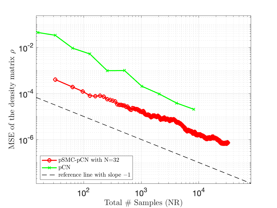
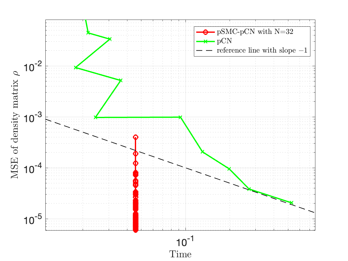
Figure 7: Convergence of the quantum state tomography example for $m=6$ and $d=16$. In pSMC, the number of mutation steps is $M=d$; in pCN, the number of burn-in samples is $0$. For both methods, the number of states is $S=10$.

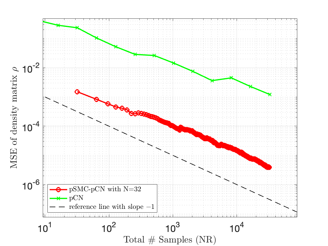
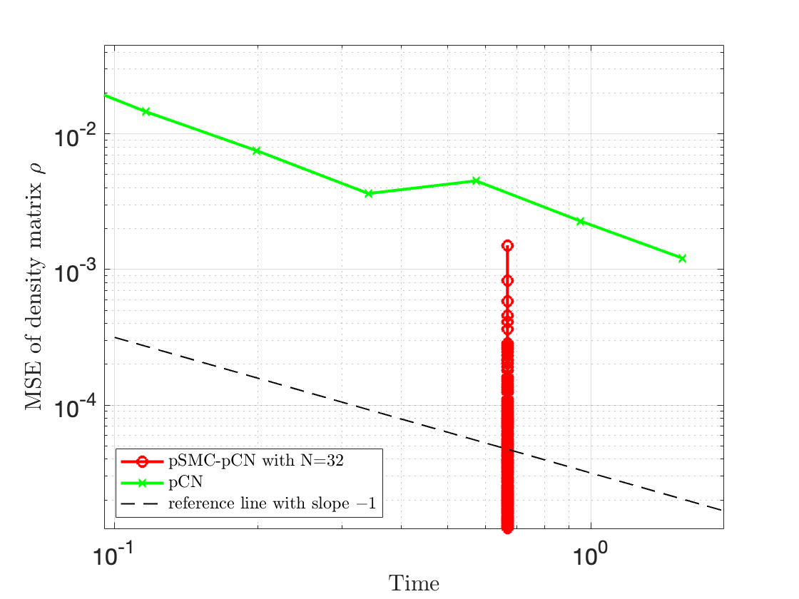
Figure 8: Convergence of the quantum state tomography example for $m=36$ and $d=64$. In pSMC, the number of mutation steps is $M=d$; in pCN, the number of burn-in samples is $0$. For both methods, the number of states is $S=10$.

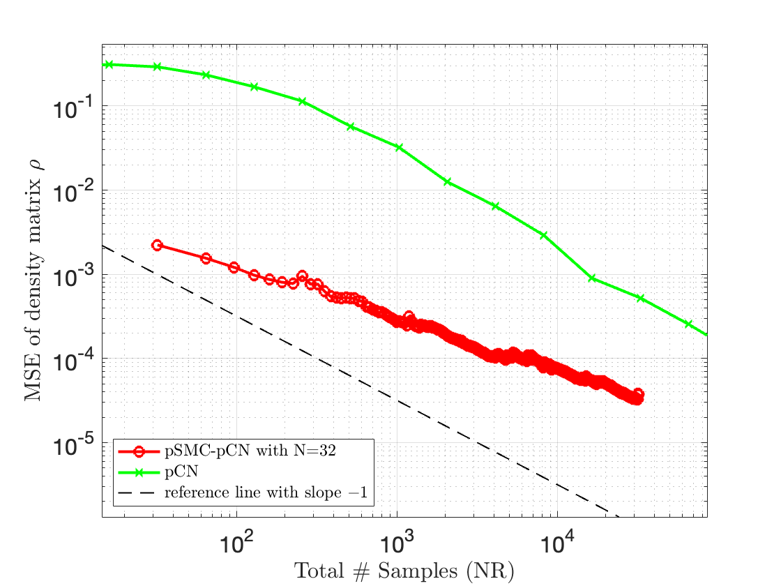
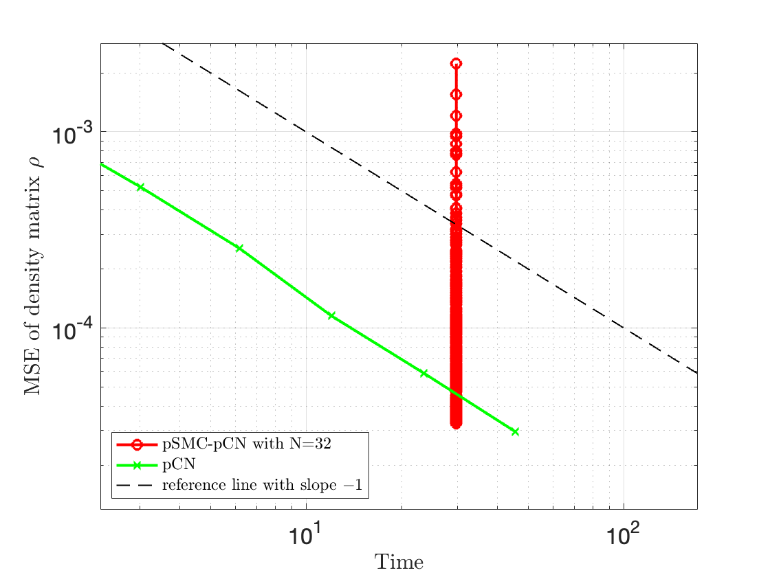
Figure 9: Convergence of the quantum state tomography example for $m=216$ and $d=256$. In pSMC, the number of mutation steps is $M=d$; in pCN, the number of burn-in samples is $0$. For both methods, the number of states is $S=10$.

We compare pSMC-pCN (with $N=32$) and pCN for $Q=1,2,3$ qubits, i.e. $(d,m)=(16,6),(64,36),(256,216)$. The quantity of interest is $\varphi=\rho$. See Figures 7, 8 and 9. The expected $1/NR$ convergence rate for pSMC is verified in the left plots in the above figures. The right plots in those figures represent the strong scaling property in pSMC and the crossover point is shown in Table 3.

4.3 Bayesian Neural Network Examples

HMC has gained widespread acceptance and favour in high-dimensional models, like the neural networks. In this section, we compare pSMC-HMC with HMC using BNN examples with similar settings cited in Cobb and Jalaian [2021].

Suppose we have data set $\mathcal{D}=\{(x_{1},y_{1}),...,(x_{m},y_{m})\}$, where $x_{i}\in\mathbb{R}^{n}$ are inputs associated to output labels $y_{i}\in\mathsf{Y}$. Let $D\in\mathbb{N}$, $(n_{0},...,n_{D})\in\mathbb{N}^{D+1}$ with $n_{0}=n$ for the input layer. Let weights be $A_{i}\in\mathbb{R}^{n_{i}\times n_{i-1}}$ and biases be $b_{i}\in\mathbb{R}^{n_{i}}$ for $i\in\{1,...,D\}$, we denote $\theta:=((A_{1},b_{1}),...,(A_{D},b_{D}))$. The layer is defined by

$$g_{1}(x,\theta) :=A_{1}x+b_{1},$$

$$g_{d}(x,\theta) :=A_{i}\sigma_{n_{i-1}}(g_{i-1}(x))+b_{i},\ \ i\in\{2,...,D-1\},$$

$$g(x,\theta) :=A_{D}\sigma_{n_{D-1}}(g_{D-1}(x))+b_{D},$$

where $\sigma_{i}(u):=(\nu(u_{1}),...,\nu(u_{i}))^{T}$ with ReLU activation $\nu(u)=\max\{0,u\}$.

In the regression example, we have $\mathsf{Y}=\mathbb{R}^{n_{D}}$ and can assume the data as follows, in which the data is defined in a continuous space,

$$y_{i}=g(x_{i},\theta)+\nu_{i},\ \epsilon\sim N(0,\sigma^{2}I),$$ (16)

where $i=\{1,...,m\}$. Then the likelihood for the regression problem (16) can be computed as

$$\mathcal{L}(\theta)=\prod_{i=1}^{m}\exp(-\frac{1}{2\sigma^{2}}\left\lVert y_{i}-g(x_{i},\theta)\right\rVert^{2}).$$

In the discrete data set, like the classification problems, we have $\mathsf{Y}=\{1,...,K\}$ and $n_{D}=K$, then we instead define the so-called softmax function as

$$h_{k}(x,\theta)=\frac{\exp(g_{k}(x,\theta))}{\sum_{j=1}^{K}\exp(g_{j}(x,\theta))},\ k\in\mathsf{Y},$$ (17)

and define $h(x,\theta)=(h_{1}(x,\theta),...,h_{K}(x,\theta))$ as a categorical distribution on $K$ outcomes based on data $x$. Then we assume that $y_{i}\sim h(x_{i})$ for $i=\{1,...,m\}$.

Now, the likelihood for the classification problem (17) can be computed as

$$\mathcal{L}(\theta)=\prod_{i=1}^{m}\prod_{k=1}^{K}h_{k}(x_{i},\theta)^{\mathds{1}_{[y_{i}=k]}},$$

where $\mathds{1}_{[y_{i}=k]}=1$ if $y_{i}=k$ and $0$ otherwise.

Given a Gaussian prior $\pi_{0}=N(0,I)$, the posterior distribution of $\theta$ is

$$\pi(\theta)\propto\mathcal{L}(\theta)\pi_{0}(\theta).$$ (18)

In the following examples, the QOI is interpreted as $\varphi=g$ in the regression problem and as the softmax function of the output, $\varphi=h$, in the classification problem. Rather than considering MSE as in the regression example, the mean centred cross-entropy (KL-divergence) is used as metric between the estimated Bayesian ground truth $\varphi_{g}$ and the Bayesian estimators $\hat{\varphi}$ in the classification cases as follows

$$L(\varphi_{g},\hat{\varphi})=\sum_{i=1}^{K}\varphi_{g,i}\log(\varphi_{g,i})-\sum_{i=1}^{K}\varphi_{g,i}\log(\hat{\varphi}_{i}).$$

4.3.1 Iris Classification Example

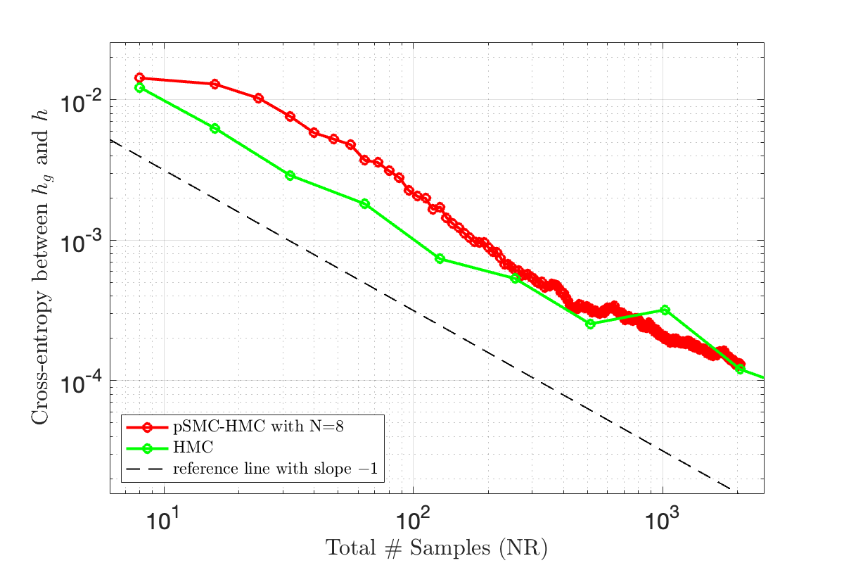
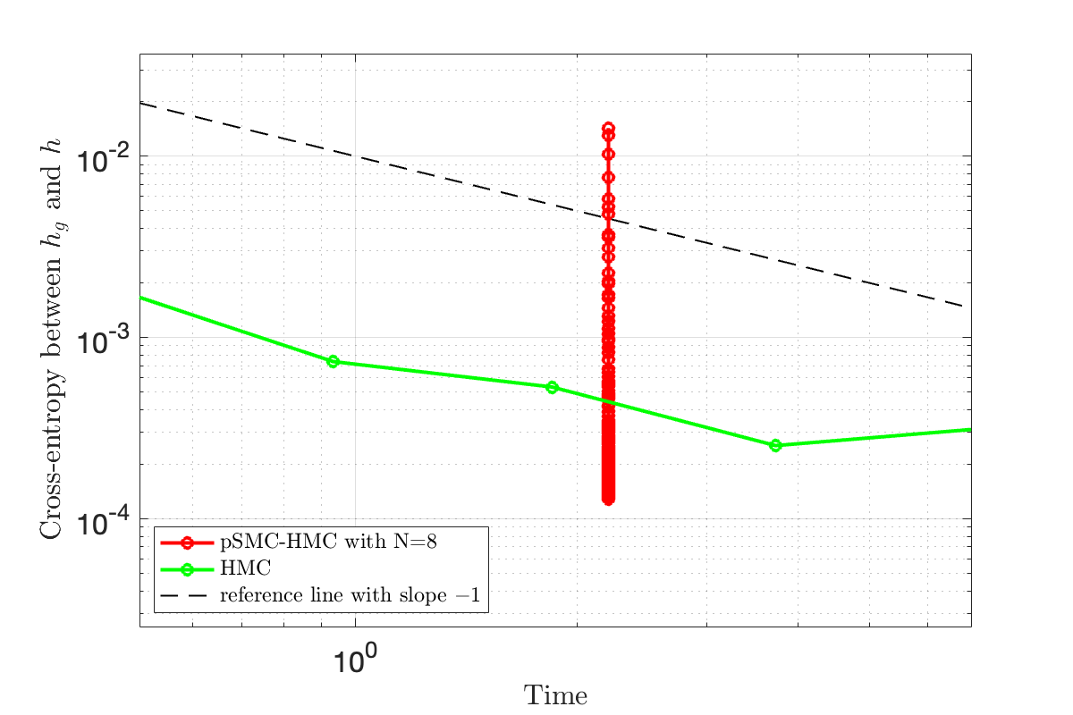
Figure 10: Convergence of the iris classification example. For both methods, the number of realizations is $10$, $L=20$, $M=1$, $\Delta=0.1$, $M_{0}=I$.

Consider a fully connected deep neural network with only one layer for learning a three-class classification problem on iris data set, that is $D=1$, $n_{0}=4$ and $n_{1}=K=3$, then the dimension of the parameter $\theta$ in neural network is $d=15$. There are $150$ data points in the iris data set, with the first $m=50$ be the training set and the remaining $100$ be the testing set. The precision parameter in likelihood is $\sigma=1$. We take $L=20$, $M=1$, $\Delta t=0.1$ and $M_{0}=I$ in HMC. The convergence results are shown in Figure 10 and crossover point is given in table 3.

4.3.2 MNIST Classification Example

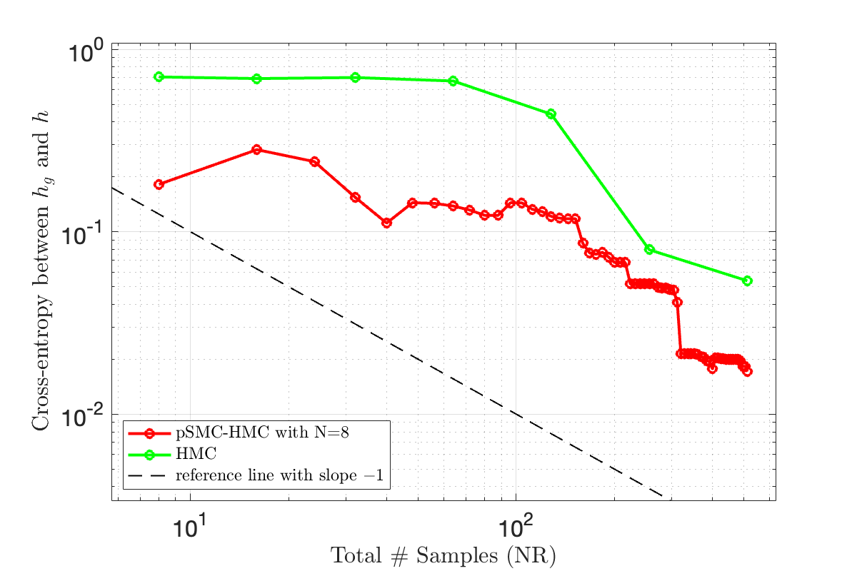
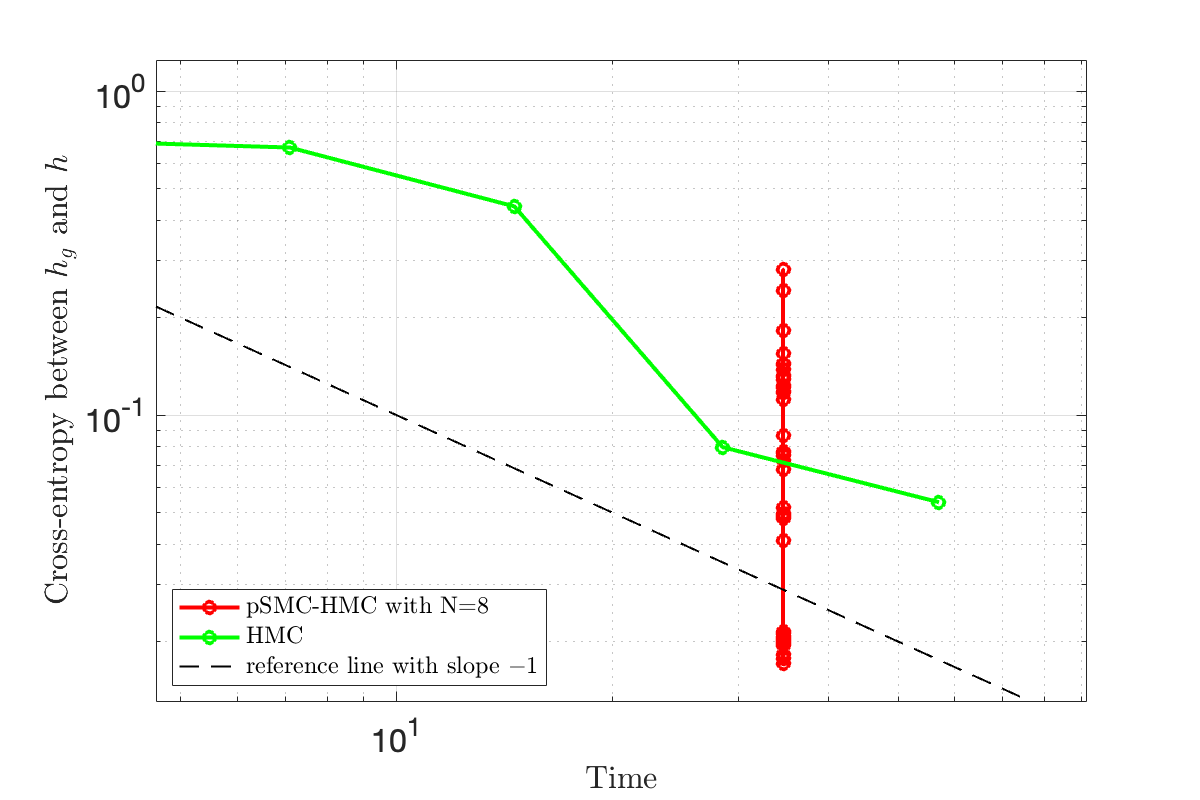
Figure 11: Convergence of the MNIST classification example. For both methods, the number of realizations is $10$, $L=20$, $M=1$, $\Delta t=0.001$, $M_{0}=0.01I$.

Now, we consider a convolution neural network with two convolution layers followed by two fully connected layers, each convolution layer with $5$ input channels and output channels, $5\times 5$ kernel and stride as $1$. Then the dimensional of parameter $\theta$ is $d=1177$. Using this neural network, we intend to learn a binary classification problem on the MNIST data set by taking the image for "0" and "1". We take the first $m=50$ images for training and following $100$ images for testing. The precision parameter in likelihood is $\sigma=1$. We take $L=20$, $M=1$, $\Delta t=0.001$ and $M_{0}=0.01I$ in HMC. The convergence results are shown in Figure 11 and crossover point is given in table 3.

5 Conclusion

The pSMC method has been introduced and proven to deliver parallel strong scaling, leading to a more practically applicable class of consistent Bayesian methods. In particular, any MCMC kernel can be plugged into pSMC and the efficiency of MCMC is preserved, while asynchronous parallel processing can be easily and straightforwardly leveraged with full parallel efficiency. This property has been verified and illustrated on a range of numerical examples in the context of machine learning. Most notably, this paves the way to high-accuracy optimal Bayesian solution to larger problems than were accessible before. It is very exciting future work to really push the limits of this method with modern HPC.

Appendix A Techniques for pSMC in practice

It is worth noting that when computing the likelihoods in a single SMC in practice, it may occur computational small numbers that the computer will recognize as 0. Fortunately, if one takes the logarithm of the number, the computer can store much smaller values. So, instead of using the likelihood itself, we store and use the log-likelihood, taking the exponential as needed. We use log-likelihood for unnormalized weights and adjust it with a constant for the small number of importance sampling weights. An additional trick is provided below to further avoid the small computational number issue when calculating the constant in the parallel SMC estimator (9).

The procedure is defined as follows: for core $r=1,...,R$,

$$Z^{N,r} =\prod_{j=1}^{J}\sum_{i=1}^{N}\omega_{j}^{i,r}=\prod_{j=1}^{J}\Delta K_{j}^{r}\Delta\hat{Z}_{j}^{r}=K^{r}\hat{Z}^{r},$$

where $\Delta K_{j}^{r}=\exp(\max_{i}\log(w_{j}^{i,r}))$ and $K^{r}=\prod_{j=1}^{J}\Delta K_{j}^{r}$; $\Delta{\hat{Z}}_{j}^{r}=\sum_{i=1}^{N}\hat{w}_{j}^{i,r}=\sum_{i=1}^{N}\exp(\log(w_{j}^{i,r})-\max_{i}\log(w_{j}^{i,r}))$ and $\hat{Z}^{r}=\prod_{j=1}^{J}\Delta\hat{Z}_{j}^{r}$. For the small number of importance sampling weights $w_{j}^{i,r}$, we work with log-likelihood for unnormalized weights and modify it with a constant $\hat{w}_{j}^{i,r}$.

Using the same trick again on the normalized constant over $R$ cores, we have, for core $r$,

$$Z^{N,r}=K^{r}\hat{Z}^{r}=\exp(\log(\hat{Z}^{r})+\log(K^{r})-\log(K))K,$$

where $\log(K)=\max_{r}(\log(\hat{Z}^{r})+\log(K^{r}))$. Since the term $K$ will be cancelled out as we compute the parallel SMC estimator, so we only need the term $\exp(\log(\hat{Z}^{r})+\log(K^{r})-\log(K))$, which could further avoid the computational error due to the small number $K$.

Appendix B Parameterization of $\rho(\theta)$ in QST

The $2^{Q}\times 2^{Q}$ density matrix $\rho(\theta)$ are parameterized by a given parameter $\theta$ with $4(2^{Q})^{2}$ non-negative real numbers distributed from the standard normal distribution. The first $2(2^{Q})^{2}$ numbers populate the real and imaginary parts of a $2^{Q}\times 2^{Q}$ matrix which through the Mezzadri algorithm is converted to a $2^{Q}\times 2^{Q}$ unitary $U$ [Mezzadri, 2006]. One can construct $U$ with the QR decomposition routines:

1. Construct a $2^{Q}\times 2^{Q}$ complex random matrix $D$ by the other $2(2^{Q})^{2}$ entries left in $\theta$.

2. Use QR decomposition to get $D=BP$.

3. Create the diagonal matrix $P_{\text{sign}}=\text{diag}(\frac{p_{11}}{|p_{11}|},...,\frac{p_{2^{Q}2^{Q}}}{|p_{2^{Q}2^{Q}}|})$, where $p_{ii}=[P]_{ii}$ for $i=1,2,3,...,2^{Q}$.

4. Construct the unitary matrix $U$ as $U=BP_{\text{sign}}$.

The second $2(2^{Q})^{2}$ parameters fill a complex $2^{Q}\times 2^{Q}$ matrix $C$, then $\rho(\theta)$ can be constructed following Al Osipov et al. [2010]:

$$\rho(\theta)=\frac{(I_{2^{Q}}+U)CC^{\text{H}}(I_{2^{Q}}+U^{\text{H}})}{\text{Tr}[(I_{2^{Q}}+U)CC^{\text{H}}(I_{2^{Q}}+U^{\text{H}})]}.$$

Appendix C Proofs

The proofs of the various results in the paper are presented here, along with restatements of the results.

C.1 Proof relating to Lemma 3.4

Lemma 4.4 Assume Assumption 3.1 and 3.2. Then, for any $J\in\mathbb{N}$, there is a $C>0$ such that for any $N,R\in\mathbb{N}$, suitable $\zeta:\mathsf{\Theta}\rightarrow\mathbb{R}$,

$$\mathbb{E}[(F^{N,R}(\zeta)-f(\zeta))^{2}]\leq\frac{C|\zeta|_{\infty}^{2}}{NR}.$$

Proof.

$$\mathbb{E}[(F^{N,R}(\zeta)-f(\zeta))^{2}] =\mathbb{E}\bigg{[}\bigg{(}\frac{1}{R}\sum_{r=1}^{R}(f^{N,r}(\zeta)-f(\zeta))\bigg{)}^{2}\bigg{]}$$

$$=\frac{1}{R^{2}}\mathbb{E}\bigg{[}\sum_{r=1}^{R}(f^{N,r}(\zeta)-f(\zeta))^{2}+\sum_{r=1}^{R}\sum_{r^{\prime}=1}^{R}(f^{N,r}(\zeta)-f(\zeta))(f^{N,r^{\prime}}(\zeta)-f(\zeta))\bigg{]}$$

$$=\frac{1}{R^{2}}\sum_{r=1}^{R}\mathbb{E}[(f^{N,r}(\zeta)-f(\zeta))^{2}]+\frac{1}{R^{2}}\sum_{r=1}^{R}\sum_{r^{\prime}=1}^{R}\mathbb{E}[(f^{N,r}(\zeta)-f(\zeta))]\mathbb{E}[(f^{N,r^{\prime}}(\zeta)-f(\zeta))].$$ (19)

By Proposition 3.3, three expectation terms in (19) are expressed as follows

$$\mathbb{E}[(f^{N,r}(\zeta)-f(\zeta))^{2}]\leq\frac{C|\zeta|_{\infty}^{2}}{N},\ \mathbb{E}[(f^{N,r}(\zeta)-f(\zeta))]=0.$$

Then, we conclude

$$\mathbb{E}[(F^{N,R}(\zeta)-f(\zeta))^{2}]\leq\frac{C|\zeta|_{\infty}^{2}}{NR}.$$

∎

C.2 Proof relating to Theorem 3.5

Theorem 4.5 Assume Assumption 3.1 and 3.2. Then, for any $J\in\mathbb{N}$, there exists a $C_{\varphi}>0$, which depends on $\varphi$, such that for any $R\in\mathbb{N}$,

$$\mathbb{E}[(\hat{\varphi}_{\text{pSMC}}-\pi(\varphi))^{2}]\leq\frac{C_{\varphi}}{NR}.$$ (20)

Then the strong scaling in the parallel SMC is described as the MSE defined in (20) decreases as $1/R$ for $R$ nodes, for suitable variables value ($M$,$N$,$J$), with constant time.

Proof.

$$\mathbb{E}[(\hat{\varphi}_{\text{pSMC}}-\pi(\varphi))^{2}] =\mathbb{E}\bigg{[}\bigg{(}\frac{F^{N,R}(\varphi)}{F^{N,R}(1)}-\frac{f(\varphi)}{f(1)}\bigg{)}^{2}\bigg{]}$$

$$=\mathbb{E}\bigg{[}\bigg{(}\frac{F^{N,R}(\varphi)}{F^{N,R}(1)}-\frac{F^{N,R}(\varphi)}{f(1)}+\frac{F^{N,R}(\varphi)}{f(1)}-\frac{f(\varphi)}{f(1)}\bigg{)}^{2}\bigg{]}$$

Applying Cauchy-Schwartz inequality, we have

$$\leq 2\mathbb{E}\bigg{[}\bigg{(}\frac{F^{N,R}(\varphi)}{F^{N,R}(1)}-\frac{F^{N,R}(\varphi)}{f(1)}\bigg{)}^{2}\bigg{]}+2\mathbb{E}\bigg{[}\bigg{(}\frac{F^{N,R}(\varphi)}{f(1)}-\frac{f(\varphi)}{f(1)}\bigg{)}^{2}\bigg{]}$$

$$\leq\frac{2|F^{N,R}(\varphi)|_{\infty}^{2}}{|F^{N,R}(1)|^{2}|f(1)|^{2}}\mathbb{E}[(F^{N,R}(1)-f(1))^{2}]+\frac{2}{|f(1)|^{2}}\mathbb{E}\big{[}(F^{N,R}(\varphi)-f(\varphi))^{2}\big{]}$$ (21)

Assume Assumption 3.1, there exists a $C_{\varphi}^{\prime}$ such that $\frac{2|F^{N,R}(\varphi)|_{\infty}^{2}}{|F^{N,R}(1)|^{2}|f(1)|^{2}}\leq C_{\varphi}^{\prime}$, and there exists a $C^{\prime}$ such that $\frac{2}{|f(1)|^{2}}\leq C^{\prime}$. Then, following (21), we have

$$\mathbb{E}[(\hat{\varphi}_{\text{pSMC}}-\pi(\varphi))^{2}] \leq C_{\varphi}^{\prime}\mathbb{E}[(F^{N,R}(1)-f(1))^{2}]+C^{\prime}\mathbb{E}\big{[}(F^{N,R}(\varphi)-f(\varphi))^{2}\big{]}$$

By Lemma 3.4 with $$\zeta=\varphi \zeta=1$$ and respectively, we have

$$\leq\frac{C_{\varphi}^{\prime}C}{NR}+\frac{C^{\prime}C|\varphi|_{\infty}^{2}}{NR}$$

$$\text{Let }C_{\varphi}=C_{\varphi}^{\prime}C+C^{\prime}C|\varphi|_{\infty}^{2}\text{, we have}$$

$$\leq\frac{C_{\varphi}}{NR}.$$

∎

Appendix D Figures

D.1 Gaussian cases

Figure 2: Convergence of the Gaussian case for $m=d=8$. In pSMC, the number of mutation steps is $M=10$; in pCN, the number of burn-in samples is $10000$. For both methods, the number of realizations is $100$.

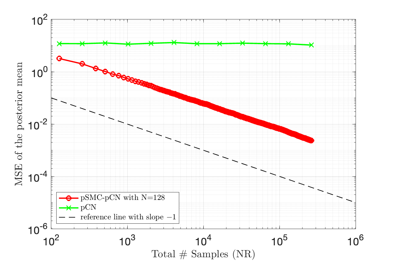
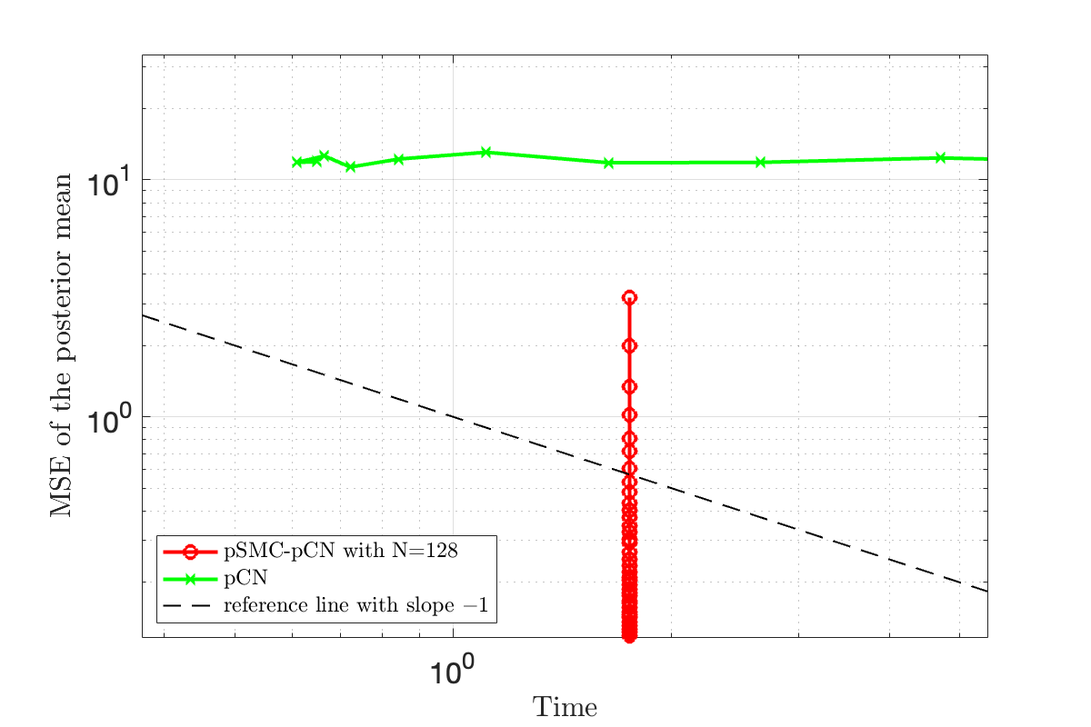
Figure 3: Convergence of the Gaussian case for $m=4$ and $d=16$. In pSMC, the number of mutation steps is $M=10$; in pCN, the number of burn-in samples is $5000$. For both methods, the number of realizations is $100$.

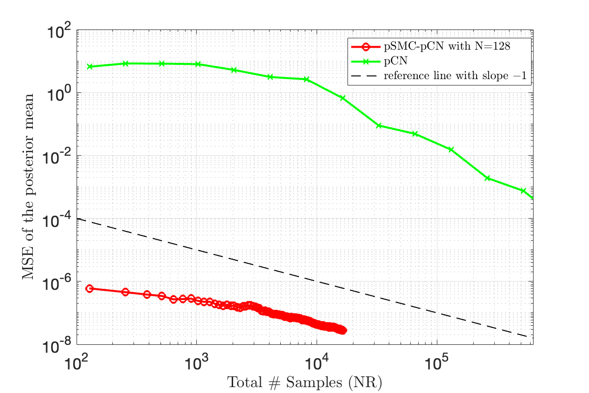
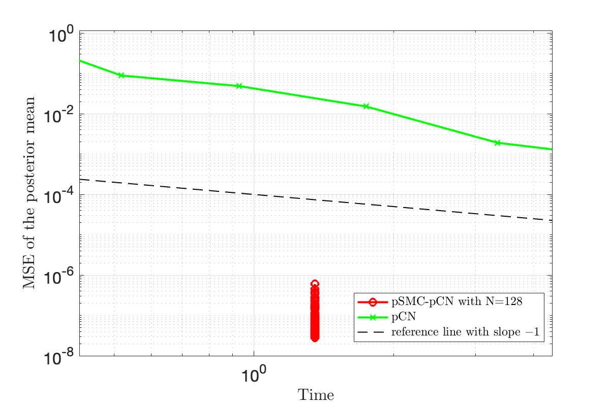
Figure 4: Convergence of the Gaussian case for $m=64$ and $d=16$. In pSMC, the number of mutation steps is $M=d$; in pCN, the number of burn-in samples is $10000$. For both methods, the numbers of realizations is $10$.

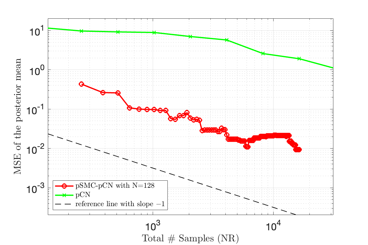
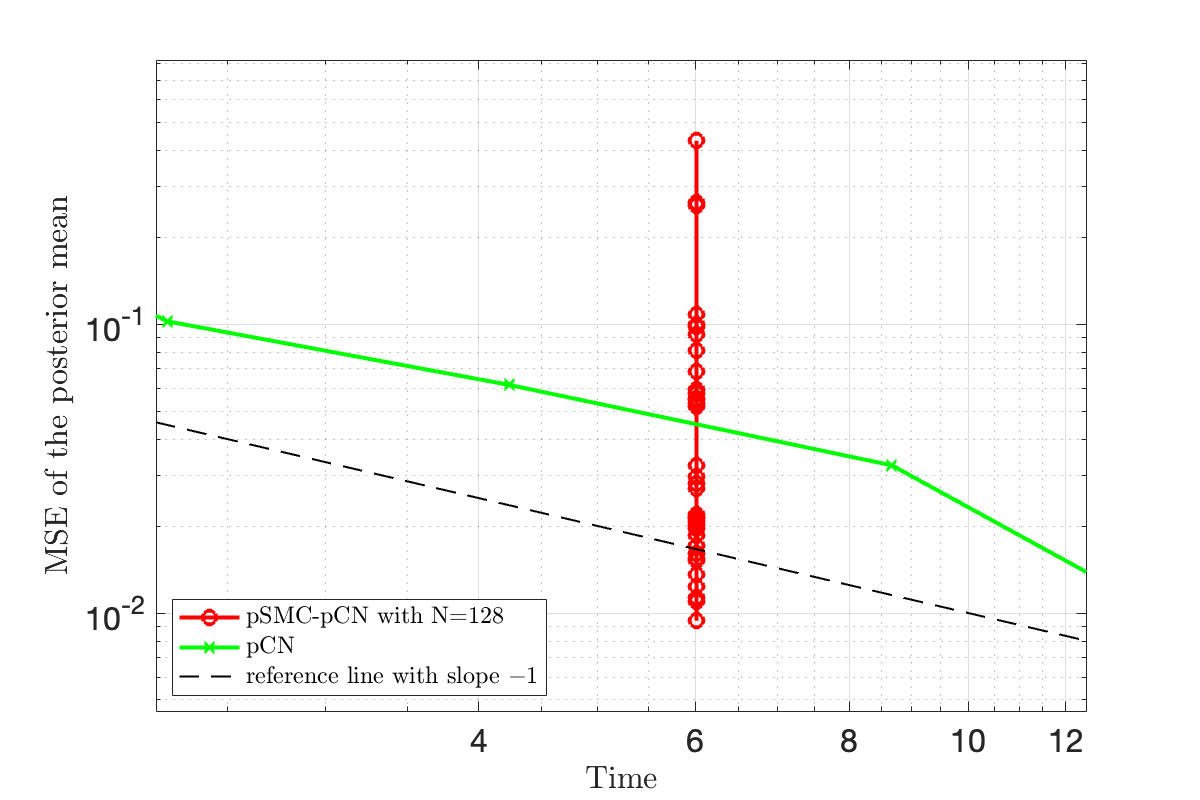
Figure 5: Convergence of the Gaussian case for $m=d=32$. In pSMC, the number of mutation steps is $M=d$; in pCN, the number of burn-in samples is $10000$. For both methods, the number of realizations is $10$.

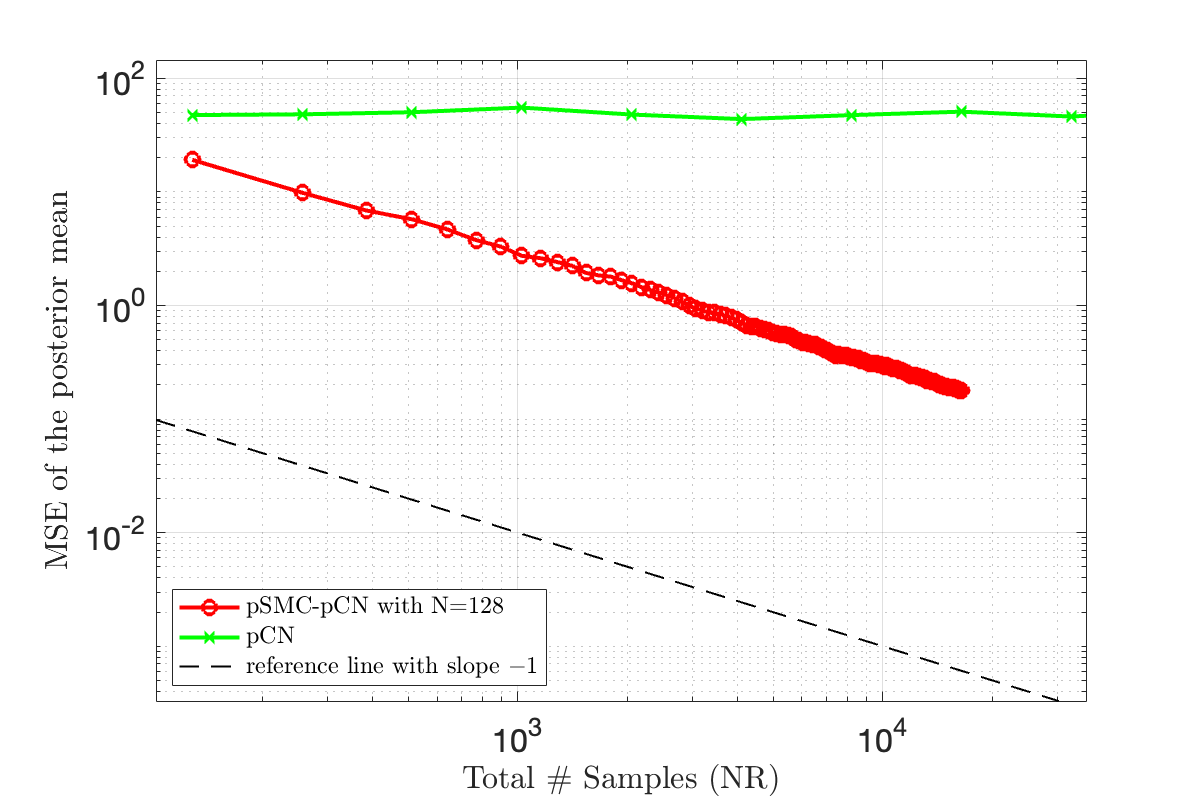
Figure 6: Convergence of the Gaussian case for $m=16$ and $d=64$. In pSMC, the number of mutation steps is $M=d$; in pCN, the number of burn-in samples is $10000$. For both methods, the number of realizations is $10$.

D.2 Quantum State Tomography problem

D.3 Bayesian Neural Network Examples

References

- Al Osipov et al. [2010] V Al Osipov, Hans-Juergen Sommers, and K Życzkowski. Random bures mixed states and the distribution of their purity. Journal of Physics A: Mathematical and Theoretical, 43(5):055302, 2010.
- Andrieu et al. [2003] Christophe Andrieu, Nando De Freitas, Arnaud Doucet, and Michael I Jordan. An introduction to mcmc for machine learning. Machine learning, 50:5–43, 2003.
- Bengio [2000] Yoshua Bengio. Probabilistic neural network models for sequential data. In Proceedings of the IEEE-INNS-ENNS International Joint Conference on Neural Networks. IJCNN 2000. Neural Computing: New Challenges and Perspectives for the New Millennium, volume 5, pages 79–84. IEEE, 2000.
- Berzuini and Gilks [2001] Carlo Berzuini and Walter Gilks. Resample-move filtering with cross-model jumps. Sequential Monte Carlo Methods in Practice, pages 117–138, 2001.
- Beskos [2014] Alexandros Beskos. A stable manifold mcmc method for high dimensions. Statistics & Probability Letters, 90:46–52, 2014.
- Beskos et al. [2017] Alexandros Beskos, Mark Girolami, Shiwei Lan, Patrick E Farrell, and Andrew M Stuart. Geometric mcmc for infinite-dimensional inverse problems. Journal of Computational Physics, 335:327–351, 2017.
- Beskos et al. [2018] Alexandros Beskos, Ajay Jasra, Kody Law, Youssef Marzouk, and Yan Zhou. Multilevel sequential monte carlo with dimension-independent likelihood-informed proposals. SIAM/ASA Journal on Uncertainty Quantification, 6(2):762–786, 2018.
- Bishop [2006] Christopher M Bishop. Pattern recognition and machine learning, volume 4. Springer, 2006.
- Blundell et al. [2015] Charles Blundell, Julien Cornebise, Koray Kavukcuoglu, and Daan Wierstra. Weight uncertainty in neural network. In International conference on machine learning, pages 1613–1622. PMLR, 2015.
- Chen et al. [2016] Yuxin Chen, David Keyes, Kody JH Law, and Hatem Ltaief. Accelerated dimension-independent adaptive metropolis. SIAM Journal on Scientific Computing, 38(5):S539–S565, 2016.
- Chopin [2002] Nicolas Chopin. A sequential particle filter method for static models. Biometrika, 89(3):539–552, 2002.
- Chopin et al. [2020] Nicolas Chopin, Omiros Papaspiliopoulos, et al. An introduction to sequential Monte Carlo, volume 4. Springer, 2020.
- Cobb and Jalaian [2021] Adam D Cobb and Brian Jalaian. Scaling hamiltonian monte carlo inference for bayesian neural networks with symmetric splitting. In Uncertainty in Artificial Intelligence, pages 675–685. PMLR, 2021.
- Cotter et al. [2013] Simon L Cotter, Gareth O Roberts, Andrew M Stuart, and David White. Mcmc methods for functions: modifying old algorithms to make them faster. 2013.
- Cui et al. [2016] Tiangang Cui, Kody JH Law, and Youssef M Marzouk. Dimension-independent likelihood-informed mcmc. Journal of Computational Physics, 304:109–137, 2016.
- Dai et al. [2022] Chenguang Dai, Jeremy Heng, Pierre E Jacob, and Nick Whiteley. An invitation to sequential monte carlo samplers. Journal of the American Statistical Association, 117(539):1587–1600, 2022.
- Del Moral [2004] Pierre Del Moral. Feynman-kac formulae. Springer, 2004.
- Del Moral et al. [2006] Pierre Del Moral, Arnaud Doucet, and Ajay Jasra. Sequential monte carlo samplers. Journal of the Royal Statistical Society Series B: Statistical Methodology, 68(3):411–436, 2006.
- Duane et al. [1987] Simon Duane, Anthony D Kennedy, Brian J Pendleton, and Duncan Roweth. Hybrid monte carlo. Physics letters B, 195(2):216–222, 1987.
- Gal and Ghahramani [2016] Yarin Gal and Zoubin Ghahramani. Dropout as a bayesian approximation: Representing model uncertainty in deep learning. In international conference on machine learning, pages 1050–1059. PMLR, 2016.
- Gelfand and Smith [1990] Alan E Gelfand and Adrian FM Smith. Sampling-based approaches to calculating marginal densities. Journal of the American statistical association, 85(410):398–409, 1990.
- Geyer [1992] Charles J Geyer. Practical markov chain monte carlo. Statistical science, pages 473–483, 1992.
- Gilks and Berzuini [2001] Walter R Gilks and Carlo Berzuini. Following a moving target—monte carlo inference for dynamic bayesian models. Journal of the Royal Statistical Society: Series B (Statistical Methodology), 63(1):127–146, 2001.
- Haario et al. [2001] Heikki Haario, Eero Saksman, and Johanna Tamminen. An adaptive metropolis algorithm. Bernoulli, pages 223–242, 2001.
- Hastings [1970] W Keith Hastings. Monte carlo sampling methods using markov chains and their applications. 1970.
- Hinton et al. [1986] Geoffrey E Hinton, Terrence J Sejnowski, et al. Learning and relearning in boltzmann machines. Parallel distributed processing: Explorations in the microstructure of cognition, 1(282-317):2, 1986.
- Houlsby et al. [2011] Neil Houlsby, Ferenc Huszár, Zoubin Ghahramani, and Máté Lengyel. Bayesian active learning for classification and preference learning. arXiv preprint arXiv:1112.5745, 2011.
- Jacob et al. [2020] Pierre E Jacob, John O’Leary, and Yves F Atchadé. Unbiased markov chain monte carlo methods with couplings. Journal of the Royal Statistical Society Series B: Statistical Methodology, 82(3):543–600, 2020.
- Jarzynski [1997] Christopher Jarzynski. Equilibrium free-energy differences from nonequilibrium measurements: A master-equation approach. Physical Review E, 56(5):5018, 1997.
- Law [2014] Kody JH Law. Proposals which speed up function-space mcmc. Journal of Computational and Applied Mathematics, 262:127–138, 2014.
- Leimkuhler and Reich [2004] Benedict Leimkuhler and Sebastian Reich. Simulating hamiltonian dynamics. Number 14. Cambridge university press, 2004.
- Lukens et al. [2020] Joseph M Lukens, Kody JH Law, Ajay Jasra, and Pavel Lougovski. A practical and efficient approach for bayesian quantum state estimation. New Journal of Physics, 22(6):063038, 2020.
- Lukens et al. [2021] Joseph M Lukens, Kody JH Law, and Ryan S Bennink. A bayesian analysis of classical shadows. npj Quantum Information, 7(1):113, 2021.
- MacKay [1992] David JC MacKay. A practical bayesian framework for backpropagation networks. Neural computation, 4(3):448–472, 1992.
- Metropolis et al. [1953] Nicholas Metropolis, Arianna W Rosenbluth, Marshall N Rosenbluth, Augusta H Teller, and Edward Teller. Equation of state calculations by fast computing machines. The journal of chemical physics, 21(6):1087–1092, 1953.
- Mezzadri [2006] Francesco Mezzadri. How to generate random matrices from the classical compact groups. arXiv preprint math-ph/0609050, 2006.
- Murphy [2012] Kevin P Murphy. Machine learning: a probabilistic perspective. 2012.
- Neal [1998] Radford Neal. Regression and classification using gaussian process priors. Bayesian statistics, 6:475, 1998.
- Neal [1993] Radford M Neal. Bayesian learning for neural networks, volume 118. Springer Science & Business Media, 1993.
- Neal [2001] Radford M Neal. Annealed importance sampling. Statistics and computing, 11:125–139, 2001.
- Neal et al. [2011] Radford M Neal et al. Mcmc using hamiltonian dynamics. Handbook of markov chain monte carlo, 2(11):2, 2011.
- Ng and Jordan [1999] Andrew Ng and Michael Jordan. Approximate inference a lgorithms for two-layer bayesian networks. Advances in neural information processing systems, 12, 1999.
- Robert et al. [1999] Christian P Robert, George Casella, and George Casella. Monte Carlo statistical methods, volume 2. Springer, 1999.
- Roberts and Tweedie [1996] Gareth O Roberts and Richard L Tweedie. Exponential convergence of langevin distributions and their discrete approximations. Bernoulli, pages 341–363, 1996.
- Rudolf and Sprungk [2018] Daniel Rudolf and Björn Sprungk. On a generalization of the preconditioned crank–nicolson metropolis algorithm. Foundations of Computational Mathematics, 18:309–343, 2018.
- Vergé et al. [2015] Christelle Vergé, Cyrille Dubarry, Pierre Del Moral, and Eric Moulines. On parallel implementation of sequential monte carlo methods: the island particle model. Statistics and Computing, 25(2):243–260, 2015.
- Whiteley et al. [2015] Nick Whiteley, Anthony Lee, and Kari Heine. On the role of interaction in sequential monte carlo algorithms. Bernoulli, 22(1):494–529, 2015.
- Zahm et al. [2022] Olivier Zahm, Tiangang Cui, Kody Law, Alessio Spantini, and Youssef Marzouk. Certified dimension reduction in nonlinear bayesian inverse problems. Mathematics of Computation, 91(336):1789–1835, 2022.