Schrödinger Connections: From Mathematical Foundations Towards Yano-Schrödinger Cosmology

Lehel Csillag
Ludwig Maximillian University Munich, csillag.lehel@physik.uni-muenchen.de
Technical University Munich, lehel.csillag@tum.de
Babe\textcommabelows-Bolyai University, csillag.lehel@stud.ubbcluj.ro
Abstract

In the present paper we introduce a novel coordinate-free formulation of Schrödinger connections, which are a special class of affine connections, first considered by Schrödinger. After recasting some basic properties in a differential geometric language, we show that Schrödinger connections can be realized through torsion, non-metricity or both. Considering a semi-symmetric type of torsion and a Weyl type non-metricity, the curvature tensors of Weyl-Schrödinger, Yano-Schrödinger and Friedmann-Weyl-Schrödinger connections are calculated. With the help of a de Sitter type FLRW metric and a Yano-Schrödinger connection, we construct for the first time in the literature an explicit example of a non-static Einstein manifold realized by torsion. Having presented the mathematical foundations, we propose a geometric generalization of standard general relativity based on Yano-Schrödinger geometry. After formulating the Einstein equations, we derive the Friedmann equations and obtain analytical de Sitter solutions. The physical feasability of the proposed theory is tested by considering a cosmological model in which matter is conserved. The theoretical predictions of Yano-Schrödinger gravity are compared with observational data for the Hubble function and with the standard $\Lambda$CDM paradigm. Our results show that Yano-Schrödinger gravity could be a plausible alternative to standard general relativity.

1 Introduction

The advancement of early 20th-century theoretical physics was closely intertwined with developments in mathematics. General relativity exemplifies this, being a product of collaborative efforts between mathematicians and physicists. Einstein and Hilbert’s theory presented an elegant geometric perspective on gravity to physicists, while simultaneously opening up new research domains like geometric analysis for mathematicians.

During the early days of general relativity, mathematicians identified two key mathematical premises of Einstein’s theory: metric compatibility and torsion-freeness of the affine connection. These conditions uniquely define the Levi-Civita connection. This realization led mathematicians to propose extensions to Einstein’s theory, by either giving up on metric-compatibility or integrating torsion. Among these, Weyl and Cartan are recognized for their significant contributions [1, 2, 3, 4, 5].

Physicists, aiming for distinct objectives [6], also suggested modifications to Einstein’s theory by incorporating torsion and non-metricity. Interestingly, in 1924, just before his death, Friedmann, renowned for his influential cosmological equations, introduced a new connection, which he called the semi-symmetric connection [7].

This connection remained mostly unnoticed by physicists, until recently. In [8], a unified field theory was proposed, which is based on a semi-symmetric connection. Zangiabadi and Zahari mention that semi symmetric connections could also describe a motion on the surface of the earth. If the movement is such that the person is always facing a definite point, like the North pole, then this displacement is semi-symmetric and metric [9, 10].

On the other hand, the mathematical aspects of semi-symmetric connections have been thoroughly examined [11, 12, 13, 14, 15, 16, 17]. These investigations came as a follow up of Kentaro Yano’s foundational work [18], in which a geometric, coordinate-free description of semi-symmetric metric connections is presented.

Despite their interesting mathematical properties, semi-symmetric connections lack a main physical requirement. They do not preserve lengths of autoparallely transported curves. The same issue is also present in other modified gravity theories, most notably in Weyl’s unification theory [19]. Weyl, based on London’s work [20], showed that a satisfactory theory of electromagnetism can be obtained, if the scale factor is replaced by a complex phase. This is the origin of the well-known $U(1)$ gauge theory [21].

Einstein’s objections for the non-preservation of length in this geometry has lead to the abandonment of the theory in the physics community, until recently. In a series of papers [22, 23, 24, 25, 26], a novel perspective on Weyl geometry was introduced, in which a scalar degree of freedom was extracted by linearizing the action with the help of an auxiliary scalar field. The physical implications of this theory were thoroughly studied in [27, 28, 29, 30, 31].

Interestingly, Schrödinger found a general affine connection that ensures the preservation of lengths during autoparallel transport. In a manner similar to the semi-symmetric connection, Schrödinger’s connection has also been overlooked in both mathematical and physics research, despite its remarkable property of being able to overcome Einstein’s objections. It has been reassessed from a physics standpoint, with Klemm and Ravera introducing a three-dimensional metric affine gravity theory, whose field equations give rise to a Schrödinger connection [32]. Additionally, physically realistic cosmological models within a Weyl-Schrödinger type geometry have been investigated in a recent paper [33].

The present work has two objectives, which could be interesting for both mathematicians and physicists. For the mathematical community, we would like to introduce Schrödinger connections in a coordinate-free manner, providing a basis for further studies. Our secondary objective is to reconsider the semi-symmetric connection through Schrödinger’s perspective and test its viability to explain observational data.

This paper is organized as follows. Section 2 provides a novel, geometric and coordinate-free exposition of Schrödinger connections. Within this section, in 2.1 some physically remarkable properties of Schrödinger connections are presented. In subsection 2.2 the focus shifts to providing examples of Schrödinger connections, culminating in theorem 2.10. The mathematical exposition ends by presenting the curvature tensors for a general Schrödinger connection. Section 3 is dedicated to expressing Schrödinger connections in terms more familiar to the physics community. We start by showing that our general results from section 2 reproduce some formulae used in the physics literature, then move on to compute the curvature tensors of specific Schrödinger geometries. An example of particular interest is the Yano-Schrödinger connection, because it is the physically reasonable version of the semi-symmetric connection considerd by Friedmann, as it preserves lengths of autoparallelly transported curves. Within this geometry, in subsection 3.2, through theorem 3.10 we provide for the first time in the literature an explicit example of an Einstein manifold with torsion, whose metric is not static. Section 4 is devoted to show the physical plausability of Yano-Schrödinger connections. We propose a generalization of standard general relativity, by considering the Einstein field equations in Yano-Schrödinger geometry. We derive the Friedmann equations, in which additional terms appear, due to the semi-symmetric type of torsion. These terms are interpreted as a form of geometric dark energy, validated through comparison with observational data. We then find analytical de Sitter solutions in this geometry and justify our interpretation. For this purpose, we reformulate the Friedmann equations in the redshift representation and examine a model where both ordinary matter and the additional torsion-derived terms are conserved, and we compare the model’s theoretical predictions for the Hubble function with both observational data and the standard $\Lambda$CDM paradigm. A summary of results, outlook and further research perspectives are provided in section 5. Some algebraic and calculational details can be found in A and B.

2 Mathematical Foundations of Schrödinger Geometry

Historically, Schrödinger’s goal was to find the most general affine connection $\nabla$, which preserves lengths of vectors that are autoparallelly transported. In his book [34], he concluded that this connection should be represented by the following Christoffel symbols

$$\tensor{\Gamma}{{}^{\lambda}_{\mu}{}_{\nu}}=\tensor{\gamma}{{}^{\lambda}_{\mu}{}_{\nu}}+g^{\lambda\rho}S_{\rho\mu\nu},$$ (2.1)

where $\tensor{\gamma}{{}^{\lambda}_{\mu}{}_{\nu}}$ denotes the Christoffel symbols of the Levi-Civita connection and $S_{\rho\mu\nu}$ is a tensor satisfying

$$S_{\rho\mu\nu}=S_{\rho\nu\mu},\;\;S_{(\rho\mu\nu)}=0.$$ (2.2)

For contemporary mathematicians, reading Schrödinger’s work might be challenging due to its reliance on local coordinates and outdated terminology. To bridge this gap, we reinterpret Schrödinger’s concepts using a coordinate-free, geometric approach. Let’s begin with the definition.

2.1 Geometric Definition and Physically Remarkable properties

Definition 2.1.

Let $(M,g)$ be a semi-Riemannian manifold and denote with $\overset{\circ}{\nabla}$ the Levi-Civita connection. An affine connection $\nabla$ on $M$ is called a Schrödinger connection if

$$\nabla_{X}Y=\overset{\circ}{\nabla}_{X}Y+U(-,X,Y)\;\;\forall X,Y\in\Gamma(TM),$$ (2.3)

where $U$ is a $(1,2)$ tensor-field satisfying the following two conditions for all vector fields $X,Y$ and one-forms $\omega$:

  1. $(a)$

    symmetry in last two entries

    $$U(\omega,X,Y)=U(\omega,Y,X);$$ (2.4)
  2. $(b)$

    cyclicity

    $\displaystyle U(\omega,X,Y)+U\left(\omega,Y,X\right)+U(X^{\flat},\omega^{\sharp},Y)$ (2.5)
    $\displaystyle+$ $\displaystyle U(X^{\flat},Y,\omega^{\sharp})+U(Y^{\flat},\omega^{\sharp},X)+U(Y^{\flat},X,\omega^{\sharp})=0,$

    where $X^{\flat}=g(X,-)$ and $\omega^{\sharp}=g^{-1}(\omega,-)$ are the musical isomorphisms.

Remark 2.2.

The cyclicity condition can be simplified by using symmetry. In particular, symmetry implies that

$$U(-,X,Y)=U(-,Y,X)\;\;\forall X,Y\in\Gamma(TM).$$ (2.6)

Hence, cyclicity takes the form

$$U(\omega,X,Y)+U(X^{\flat},\omega^{\sharp},Y)+U(Y^{\flat},\omega^{\sharp},X)=0.$$ (2.7)
Remark 2.3.

One could misleadingly think that Schrödinger connections are unique. This is not the case, in fact there are infinitely many. Each choice of the $(1,2)$-tensor field $U$ gives rise to a valid Schrödinger connection. To specify the Schrödinger connection, one often specifies $U$, or considers it fixed. Thus, a specified Schrödinger connection is denoted by $(\nabla,U)$.

To relate with Schrödinger’s work, we formally introduce the Schrödinger tensor, whose components coincide with (2.2).

Definition 2.4.

Let $(M,g)$ be a semi-Riemannian manifold with a given Schrödinger connection $(\nabla,U)$. The Schrödinger tensor $S$ associated to the Schrödinger connection $(\nabla,U)$ is defined as

$$S:\Gamma(TM)\times\Gamma(TM)\times\Gamma(TM)\to C^{\infty}(M),\;\;S(A,X,Y):=U(A^{\flat},X,Y).$$ (2.8)
Proposition 2.5.

Let $\nabla$ be an affine connection on a semi-Riemannian manifold $(M,g)$ of the form

$$\nabla_{X}Y=\overset{\circ}{\nabla}_{X}Y+U(-,X,Y),$$ (2.9)

where $U(-,X,Y)$ is a $(1,2)$-tensor field and $X,Y$. Then the following are equivalent:

  1. (i)𝑖(i)

    The pair $(U,\nabla)$ is a Schrödinger connection;

  2. (ii)𝑖𝑖(ii)

    For all vector fields $A,X,Y$ the Schrödinger tensor $S$ associated to $U$ satisfies

    $$S(A,X,Y)=S(A,Y,X),\;\;S(A,X,Y)+S(Y,A,X)+S(X,Y,A)=0.$$
Proof.

The proof follows immediately from the definitions provided

$$S(A,X,Y)=U\left(A^{\flat},X,Y\right)=U\left(A^{\flat},Y,X\right)=S(A,Y,X),$$
$\displaystyle S(A,X,Y)+S(Y,A,X)+S(X,Y,A)=$
$\displaystyle=$ $\displaystyle U\left(A^{\flat},X,Y\right)+U\left(Y^{\flat},A,X\right)+U\left(X^{\flat},Y,A\right)=0.$

Schrödinger connections have two remarkable properties:

  1. (S$1$)

    They are torsion-free;

  2. (S$2$)

    The length of autoparallelly transported vectors does not change.

We begin by establishing property (S$2$), as it is this characteristic that renders Schrödinger connections physically significant, making them overcome Einstein’s concerns. First, we prove a more general proposition, from which (S$2$) can be directly obtained.

Proposition 2.6.

Let $\nabla$ be an affine conneciton on a semi-Riemannian manifold $(M,g)$ of the form

$$\nabla_{X}Y=\overset{\circ}{\nabla}_{X}Y+U(-,X,Y)$$ (2.10)

for vector fields $X,Y$ and a $(1,2)$-tensor field $U$. For all vector fields $X$, which satisfy $\nabla_{X}X=0$, the following are equivalent:

  1. (i)𝑖(i)

    $\nabla_{X}(g(X,X))=0$,

  2. (ii)𝑖𝑖(ii)

    $U\left(X^{\flat},X,X\right)=0$.

Proof.

Fix an arbitrary vector field $A\in\Gamma(TM)$ and suppose it is the tangent to a $\nabla$-autoparallel curve, so that $\nabla_{A}A=0$. Observe that substituting $X=Y=A$ in equation (2.10), we get

$$\overset{\circ}{\nabla}_{A}A+U(-,A,A)=0.$$ (2.11)

Since $\overset{\circ}{\nabla}$ is the Levi-Civita connection, we have $\overset{\circ}{\nabla}g=0$, so

$\displaystyle\nabla_{A}(g(A,A))$ $\displaystyle=\overset{\circ}{\nabla}_{A}(g(A,A))$
$\displaystyle=\overset{\circ}{\nabla}_{A}g(A,A)+g\left(\overset{\circ}{\nabla}_{A}A,A\right)+g\left(A,\overset{\circ}{\nabla}_{A}A\right)$
$\displaystyle=2g\left(\overset{\circ}{\nabla}_{A}A,A\right)=-2g(U(-,A,A),A)$
$\displaystyle=-2U\left(A^{\flat},A,A\right),$

where in the last step we used equation (2.11). Hence

$$\nabla_{A}(g(A,A))=-2U\left(A^{\flat},A,A\right).$$ (2.12)

Therefore the condition that the parallel transport of $\nabla$ preserves lengths is equivalent to

$$U\left(A^{\flat},A,A\right)=0,\;\;\text{as desired}.$$

Corollary 2.7.

Schrödinger connections preserve the length of autoparallelly transported curves.

Proof.

By definition, the $(1,2)$-tensor field $U$ of a Schrödinger connection satisfies

$$U(\omega,X,Y)+U\left(X^{\flat},\omega^{\sharp},Y\right)+U\left(Y^{\flat},\omega^{\sharp},X\right)=0$$ (2.13)

for all $X,Y\in\Gamma(TM)$ and $\omega\in\Omega^{1}(M)$. Choose $X=Y=A,\omega=A^{\flat}$, so

$$U\left(A^{\flat},A,A\right)+U\left(A^{\flat},A,A\right)+U(A^{\flat},A,A)=0\iff U\left(A^{\flat},A,A\right)=0.$$

In the following, we prove (S$1$).

Proposition 2.8.

Schrödinger connections are torsion-free.

Proof.

The torsion tensor of an affine connection $\nabla$ is defined as

$$T(\omega,X,Y)=\omega(\nabla_{X}Y-\nabla_{Y}X-[X,Y]),\;\;\forall\omega\in\Omega^{1}(M),X,Y\in\Gamma(TM).$$

For Schrödinger connections, one obtains

$$T(\omega,X,Y)=\omega\left(\overset{\circ}{\nabla}_{X}Y+U(-,X,Y)-\overset{\circ}{\nabla}_{Y}X-U(-,Y,X)-[X,Y]\right),$$

which can be equivalently rewritten as

$$T(\omega,X,Y)=U(\omega,X,Y)-U(\omega,Y,X),$$ (2.14)

since the Levi-Civita connection is torsion-free. Symmetry of $U$ implies

$$T(\omega,X,Y)=0\;\;\forall\omega\in\Omega^{1}(M),X,Y\in\Gamma(TM),$$ (2.15)

thus concluding the proof. ∎

Remark 2.9.

Attention has to be paid to the preceeding proposition. While it is claimed that Schrödinger connections can be realized by torsion, it’s crucial to distinguish between the terms realized and have. A subsequent proposition will be presented, implementing Schrödinger connections via the torsion tensor of a distinct connection. However, it is essential to note that the realization of the Schrödinger connection $(\nabla,U)$ through this method does not imply that the connection itself possesses a non-vanishing torsion tensor.

2.2 Realizations Using Torsion and Non-Metricity

After exploring the fundamental properties of Schrödinger connections, we move on to present particular instances of these connections, selecting $U$ to represent either the torsion or non-metricity of a distinct affine connection. The findings of this section can be summarized in the following theorem.

Theorem 2.10 (Realization of Schrödinger Connections).

Let $\nabla$ be an affine connection $\nabla$ on a semi-Riemannian manifold $(M,g)$ of the form

$$\nabla_{X}Y=\overset{\circ}{\nabla}_{X}Y+U(-,X,Y),$$ (2.16)

where $U(-,X,Y)$ is a $(1,2)$-tensor field. Fix a different affine connection $\overset{A}{\nabla}$ with torsion tensor $\overset{A}{T}$,non-metricity $\overset{A}{Q}$ satisfying

$$\overset{A}{Q}(X,Y,Z)+\overset{A}{Q}(Z,X,Y)+\overset{A}{Q}(Y,Z,X)=0$$ (2.17)

and let $\pi,W$ be two one-forms on $M$. If $U(\omega,X,Y)$ is given by any of the following list

  1. (i)𝑖(i)

    $U(\omega,X,Y)=\frac{1}{2}\left(\overset{A}{T}\left(X^{\flat},Y,\omega^{\sharp}\right)+\overset{A}{T}\left(Y^{\flat},X,\omega^{\sharp}\right)\right)$,

  2. (ii)𝑖𝑖(ii)

    $U(\omega,X,Y)=\frac{1}{2}\left(X^{\flat}\left(\pi\left(\omega^{\sharp}\right)Y-\pi(Y)\omega^{\sharp}\right)+Y^{\flat}\left(\pi\left(\omega^{\sharp}\right)Y-\pi(X)\omega^{\sharp}\right)\right)$,

  3. $(iii)$

    $U(\omega,X,Y)=-\overset{A}{Q}\left(\omega^{\sharp},X,Y\right)$,

  4. $(iv)$

    $U(\omega,X,Y)=-2W\left(\omega^{\sharp}\right)g(X,Y)-2W(Y)g\left(\omega^{\sharp},X\right)-2W(X)g\left(\omega^{\sharp},Y\right),$

  5. $(v)$

    $\begin{aligned} U(\omega,X,Y)&=\frac{1}{2}\left(X^{\flat}\left(\pi\left(\omega^{\sharp}\right)Y-\pi(Y)\omega^{\sharp}\right)+Y^{\flat}\left(\pi\left(\omega^{\sharp}\right)Y-\pi(X)\omega^{\sharp}\right)\right)\\ &-2W\left(\omega^{\sharp}\right)g(X,Y)-2W(Y)g\left(\omega^{\sharp},X\right)-2W(X)g\left(\omega^{\sharp},Y\right),\end{aligned}$

then $\nabla$ is a Schrödinger connection.

We will dedicate the rest of the section to prove each item in the above theorem in detail.

Proposition 2.11.

Let $(M,g)$ be a semi-Riemannian manifold with an affine connection $\overset{A}{\nabla}$, whose torsion $\overset{A}{T}$ is non-vanishing. Then, the pair $(\nabla,U)$ defined by

$$U(\omega,X,Y)=\frac{1}{2}\left(\overset{A}{T}\left(X^{\flat},Y,\omega^{\sharp}\right)+\overset{A}{T}\left(Y^{\flat},X,\omega^{\sharp}\right)\right)$$ (2.18)

is a Schrödinger connection.

Proof.

To prove $(\nabla,U)$ is a Schrödinger connection, we have to verify both symmetry and cyclicity. We start with symmetry and compute

$$U(\omega,Y,X)=\frac{1}{2}\left(\overset{A}{T}\left(Y^{\flat},X,\omega^{\sharp}\right)+\overset{A}{T}\left(X^{\flat},Y,\omega^{\sharp}\right)\right).$$ (2.19)

It is evident that the right hand sides of equations (2.18) and (2.19) agree. Consequently, it follows that

$$U(\omega,Y,X)=U(\omega,X,Y),$$ (2.20)

thereby establishing symmetry. For cyclicity, we have

$$U(\omega,X,Y)=\frac{1}{2}\left({\color[rgb]{1,0,0}\overset{A}{T}\left(X^{\flat},Y,\omega^{\sharp}\right)}+{\color[rgb]{0,0,1}\overset{A}{T}\left(Y^{\flat},X,\omega^{\sharp}\right)}\right)$$ (2.21)
$$U\left(X^{\flat},\omega^{\sharp},Y\right)=\frac{1}{2}\left({\color[rgb]{0,0.75,0.16}\overset{A}{T}\left(\omega,Y,X\right)}+{\color[rgb]{0,0,1}\overset{A}{T}\left(Y^{\flat},\omega^{\sharp},X\right)}\right)$$ (2.22)
$$U\left(Y^{\flat},\omega^{\sharp},X\right)=\frac{1}{2}\left({\color[rgb]{0,0.75,0.16}\overset{A}{T}\left(\omega,X,Y\right)}+{\color[rgb]{1,0,0}\overset{A}{T}\left(X^{\flat},\omega^{\sharp},Y\right)}\right).$$ (2.23)

After summing equations (2.21), (2.22), (2.23), the right-hand side cancels out entirely, as coded in colors, thanks to the symmetries of the torsion tensor. Hence, the desired equality

$$U(\omega,X,Y)+U\left(X^{\flat},\omega^{\sharp},Y\right)+U\left(Y^{\flat},\omega^{\sharp},X\right)=0$$ (2.24)

is obtained. ∎

Corollary 2.12.

The Schrödinger tensor of a Schrödinger connection $(\nabla,U)$ implemented by torsion $\overset{A}{T}$ of an affine connection is given by

$\displaystyle S:\Gamma(TM)\times\Gamma(TM)\times\Gamma(TM)\to C^{\infty}(M)$ (2.25)
$\displaystyle S(A,X,Y)=\frac{1}{2}\left(\overset{A}{T}\left(Y^{\flat},X,A\right)+\overset{A}{T}\left(X^{\flat},Y,A\right)\right)$

In the introduction we mentioned that Kentaro Yano explored the mathematical properties of an interesting connection, with torsion of the semi-symmetric type. In the following, recalling this notion, we provide an example of a Schrödinger connection, which is realized this way.

Definition 2.13.

On a semi-Riemannian manifold $(M,g)$ a connection $\nabla$ is called semi-symmetric if there exists a one-form $\pi$ such that

$$T(\omega,X,Y)=\omega(\pi(Y)X-\pi(X)Y)\;\;\forall X,Y\in\Gamma(TM),\omega\in\Omega^{1}(M).$$
Corollary 2.14.

Given a one-form $\pi$, the pair $(\nabla,U)$ defined by

$$U(\omega,X,Y)=\frac{1}{2}\left(X^{\flat}\left(\pi\left(\omega^{\sharp}\right)Y-\pi(Y)\omega^{\sharp}\right)+Y^{\flat}\left(\pi\left(\omega^{\sharp}\right)Y-\pi(X)\omega^{\sharp}\right)\right)$$

is a Schrödinger connection, called the Yano-Schrödinger connection.

In the following, we will implement a Schrödinger connection using the non-metricity tensor, which is defined as

$$Q(X,Y,Z)=-(\nabla_{X}g)(Y,Z),\;\;\forall X,Y,Z\in\Gamma(TM).$$ (2.26)
Proposition 2.15.

Let $(M,g)$ be a semi-Riemannian manifold with an affine connection $\overset{A}{\nabla}$, whose non-metricity $\overset{A}{Q}$ is non-vanishing and satisfies

$$\overset{A}{Q}(X,Y,Z)+\overset{A}{Q}(Z,Y,X)+\overset{A}{Q}(X,Z,Y).$$ (2.27)

Then, there exists a Schrödinger connection $(\nabla,U)$, which is implemented by $\overset{A}{Q}$.

Proof.

We define the Schrödinger connection $(\nabla,U)$ as

$$U(\omega,X,Y)=-\overset{A}{Q}\left(\omega^{\sharp},X,Y\right)\;\;\forall\omega\in\Omega^{1}(M),X,Y\in\Gamma(TM).$$ (2.28)

To see that $U$ is symmetric in its last two entries, it suffices to show that the non-metricity is, which is a direct consequence of the Leibniz rule for the connection $\overset{A}{\nabla}$. For cyclicity, consider

$$U\left(Y^{\flat},\omega^{\sharp},X\right)=-\overset{A}{Q}\left(Y,\omega^{\sharp},X\right),$$ (2.29)
$$U\left(X^{\flat},\omega^{\sharp},Y\right)=-\overset{A}{Q}\left(X,\omega^{\sharp},Y\right)=-\overset{A}{Q}\left(X,Y,\omega^{\sharp}\right).$$ (2.30)

We sum up the three equations (2.28),(2.29) and (2.30). By assumption (2.27), the right hand sides vanish, so

$$U(\omega,X,Y)+U\left(Y^{\flat},\omega^{\sharp},X\right)+U\left(X^{\flat},\omega^{\sharp},Y\right)=0,$$ (2.31)

which is exactly the cyclicity condition. ∎

A notable and heavily used non-metricity in physics is the one introduced by Weyl, which is closely associated with conformal geometry. Like the semi-symmetric connection, this non-metricity is fully characterized by a one-form $W$

$$Q\left(X,Y,Z\right)=-2W(X)g(Y,Z).$$ (2.32)

This type of non-metricity gives rise to the Weyl-Schrödinger connection $(\nabla,U)$, which is specified by

$$U(\omega,X,Y)=2W\left(\omega^{\sharp}\right)g(X,Y)+2W(Y)g\left(\omega^{\sharp},X\right)+2W(X)g\left(\omega^{\sharp},Y\right).$$

Until now, we have implemented Schrödinger connections using either non-metricity or torsion independently. However, it is possible to construct them by employing both non-metricity and torsion simultaneously.

Proposition 2.16.

Let $W,\pi$ be one-forms on a semi-Riemannian manifold $(M,g)$. Then the pair $(\nabla,U)$ given by

$\displaystyle U(\omega,X,Y)$ $\displaystyle=\frac{1}{2}\left(X^{\flat}\left(\pi\left(\omega^{\sharp}\right)Y-\pi(Y)\omega^{\sharp}\right)+Y^{\flat}\left(\pi\left(\omega^{\sharp}\right)X-\pi(X)\omega^{\sharp}\right)\right)$ (2.33)
$\displaystyle-2W\left(\omega^{\sharp}\right)g(X,Y)-2W(Y)g\left(\omega^{\sharp},X\right)-2W(X)g\left(\omega^{\sharp},Y\right)$

is a Schrödinger-connection, called the Friedmann-Weyl-Schrödinger connection.

The terminology used here is purely historical and reflects the contributions of Friedmann, Schouten, Yano, and Weyl. Friedmann and Schouten introduced semi-symmetric connections, while Yano extensively studied the geometry of metric connections falling within the same class. Weyl, on the other hand, considered a specific type of non-metricity. A comprehensive overview of the connections discussed in this section can be found in Table $1$.

2.3 Curvature Tensors

We conclude the mathematical exposition by computing the curvature tensor of a general Schrödinger connection.

Proposition 2.17.

The Riemann curvature tensor of a Schrödinger connection $(\nabla,U)$ takes the form

$\displaystyle Riem(\omega,Z,X,Y)=\overset{\circ}{Riem}(\omega,Z,X,Y)+\left(\overset{\circ}{\nabla}_{X}U\right)(\omega,Y,Z)$
$\displaystyle-\left(\overset{\circ}{\nabla}_{Y}U\right)(\omega,X,Z)+U(\omega,X,U(-,Y,Z))$
$\displaystyle-U(\omega,Y,U(-,X,Z)).$

where $\overset{\circ}{{Riem}}$ denotes the Riemann tensor of the Levi-Civita connection.

Proof.

The Riemann tensor of an affine connection $\nabla$ is given by

$$Riem(\omega,Z,X,Y)=\omega\left(\nabla_{X}\nabla_{Y}Z-\nabla_{Y}\nabla_{X}Z-\nabla_{[X,Y]}Z\right)$$

To streamline the notation, we introduce the expression

$$Riem(\omega,Z,X,Y)=\omega\left(\operatorname{Riem}(-,Z,X,Y)\right).$$

In the following, we evaluate $\operatorname{Riem}(-,X,Y,Z)$ through a series of steps. We begin with the definition, then expand it in two steps using the definition of a Schrödinger connection:

$\displaystyle\operatorname{Riem}(-,Z,X,Y)=\nabla_{X}\nabla_{Y}Z-\nabla_{Y}\nabla_{X}Z-\nabla_{[X,Y]}Z$
$\displaystyle=\nabla_{X}\left(\overset{\circ}{\nabla}_{Y}Z+U(-,Y,Z)\right)-\nabla_{Y}\left(\overset{\circ}{\nabla}_{X}Z+U(-,X,Z)\right)$
$\displaystyle-\overset{\circ}{\nabla}_{[X,Y]}Z-U(-,[X,Y],Z)$
$\displaystyle=\overset{\circ}{\nabla}_{X}\left(\overset{\circ}{\nabla}_{Y}Z+U(-,Y,Z)\right)+U\left(-,X,\overset{\circ}{\nabla}_{Y}Z+U(-,Y,Z)\right)$
$\displaystyle-\overset{\circ}{\nabla}_{Y}\left(\overset{\circ}{\nabla}_{X}Z+U(-,Y,Z)\right)-U\left(-,Y,\overset{\circ}{\nabla}_{X}Z+U(-,X,Z)\right)$
$\displaystyle-\overset{\circ}{\nabla}_{[X,Y]}Z-U(-,[X,Y],Z).$

On the right-hand side, we expand the brackets using multilinearity of $U$:

$\displaystyle{\color[rgb]{0,0,1}\overset{\circ}{\nabla}_{X}\overset{\circ}{\nabla}_{Y}Z}+\overset{\circ}{\nabla}_{X}(U(-,Y,Z))+U\left(-,X,\overset{\circ}{\nabla}_{Y}Z\right)+U(-,X,U(-,Y,Z))$
$\displaystyle{\color[rgb]{0,0,1}-\overset{\circ}{\nabla}_{Y}\overset{\circ}{\nabla}_{X}Z}-\overset{\circ}{\nabla}_{Y}(U(-,X,Z))-U\left(-,Y,\overset{\circ}{\nabla}_{X}Z\right)-U(-,Y,U(-,X,Z))$
$\displaystyle{\color[rgb]{0,0,1}-\overset{\circ}{\nabla}_{[X,Y]}Z}-U(-,[X,Y],Z).$

The combined terms in blue can be identified with the Riemann tensor of the Levi-Civita connection, hence

$\displaystyle\overset{\circ}{\operatorname{Riem}}(-,Z,X,Y)+{\color[rgb]{1,0,0}\overset{\circ}{\nabla}_{X}(U(-,Y,Z))}+U\left(-,X,\overset{\circ}{\nabla}_{Y}Z\right)$
$\displaystyle+U(-,X,U(-,Y,Z)){\color[rgb]{1,0,0}-\overset{\circ}{\nabla}_{Y}(U(-,X,Z))}-U\left(-,Y,\overset{\circ}{\nabla}_{X}Z\right)$
$\displaystyle-U(-,Y,U(-,X,Z))-U(-,[X,Y],Z).$

Applying the Leibniz Rule to the terms highlighted in red yields

$\displaystyle\overset{\circ}{\operatorname{Riem}}(-,Z,X,Y)+\left(\overset{\circ}{\nabla}_{X}U\right)(-,Y,Z){\color[rgb]{0,0.6,0}+U\left(-,\overset{\circ}{\nabla}_{X}Y,Z\right)}$
$\displaystyle{\color[rgb]{0.5,0,1}+U\left(-,Y,\overset{\circ}{\nabla}_{X}Z\right)}{\color[rgb]{1,.5,0}+U\left(-,X,\overset{\circ}{\nabla}_{Y}Z\right)}+U(-,X,U(-,Y,Z))$
$\displaystyle-\left(\overset{\circ}{\nabla}_{Y}U\right)(-,X,Z){\color[rgb]{0,0.6,0}-U\left(-,\overset{\circ}{\nabla}_{Y}X,Z\right)}{\color[rgb]{1,.5,0}-U\left(-,X,\overset{\circ}{\nabla}_{Y}Z\right)}$
$\displaystyle{\color[rgb]{0.5,0,1}-U\left(-,Y,\overset{\circ}{\nabla}_{X}Z\right)}-U(-,Y,U(-,X,Z)){\color[rgb]{0,0.6,0}-U(-,[X,Y],Z)}.$

The green terms disappear due to the torsion-freeness of the Levi-Civita connection. The purple and orange terms cancel out, leaving us with

$\displaystyle\operatorname{Riem}(-,Z,X,Y)=\overset{\circ}{\operatorname{Riem}}(-,X,Y,Z)+\left(\overset{\circ}{\nabla}_{X}U\right)(-,Y,Z)$
$\displaystyle-\left(\overset{\circ}{\nabla}_{Y}U\right)(-,X,Z)+U(-,X,U(-,Y,Z))$
$\displaystyle-U(-,Y,U(-,X,Z)).$

Therefore, for the Riemann tensor, we achieve the desired result

$\displaystyle Riem(\omega,Z,X,Y)=\overset{\circ}{Riem}(\omega,Z,X,Y)+\left(\overset{\circ}{\nabla}_{X}U\right)(\omega,Y,Z)$
$\displaystyle-\left(\overset{\circ}{\nabla}_{Y}U\right)(\omega,X,Z)+U(\omega,X,U(-,Y,Z))$
$\displaystyle-U(\omega,Y,U(-,X,Z)).$

Corollary 2.18.

The Ricci curvature of a Schrödinger connection $(\nabla,U)$ is

$\displaystyle Ric(Z,Y)$ $\displaystyle=\overset{\circ}{Ric}(Z,Y)+\left(\overset{\circ}{\nabla}_{X}U\right)\left(X^{\flat},Y,Z\right)$ (2.34)
$\displaystyle-\left(\overset{\circ}{\nabla}_{Y}U\right)\left(X^{\flat},X,Z\right)+U\left(X^{\flat},X,U(-,Y,Z)\right)$
$\displaystyle-U\left(X^{\flat},Y,U(-,X,Z)\right).$
Corollary 2.19.

The Ricci scalar of a Schrödinger connection $(\nabla,U)$ is

$\displaystyle R$ $\displaystyle=\overset{\circ}{R}+\left(\overset{\circ}{\nabla}_{X}U\right)\left(X^{\flat},Y,Y\right)$ (2.35)
$\displaystyle-\left(\overset{\circ}{\nabla}_{Y}U\right)\left(X^{\flat},X,Y\right)+U\left(X^{\flat},X,U(-,Y,Y)\right)$
$\displaystyle-U\left(X^{\flat},Y,U(-,X,Y)\right).$

3 Local Description: A physicist perspective

In this section, in contrast to the earlier global approach, we choose local charts. First, we show that the coordinate expressions for Schrödinger connections implemented by non-metricity as presented in [33] can be directly obtained from our global formulae. Subsequently, we calculate and present new coordinate expressions for the curvature tensors of Yano-Schrödinger, Weyl-Schrödinger, and Friedmann-Weyl-Schrödinger geometries.

3.1 Coordinate Expressions for Curvature Tensors

The results of this subsection are summarized in the following theorem.

Theorem 3.1.

The three introduced geometries have the following curvature properties:

  1. 1.

    Yano-Schrödinger

    1. (i)𝑖(i)

      Ricci tensor: $R_{\mu\nu}=\overset{\circ}{R}_{\mu\nu}+g_{\mu\nu}\overset{\circ}{\nabla}_{\alpha}\pi^{\alpha}-\frac{1}{2}\overset{\circ}{\nabla}_{\mu}\pi_{\nu}+\overset{\circ}{\nabla}_{\nu}\pi_{\mu}-\frac{1}{2}g_{\mu\nu}\pi^{\alpha}\pi_{\alpha}-\frac{1}{4}\pi_{\nu}\pi_{\mu},$

    2. (ii)𝑖𝑖(ii)

      Ricci scalar: $R=\overset{\circ}{R}+\frac{9}{2}\overset{\circ}{\nabla}_{\mu}\pi^{\mu}-\frac{9}{4}\pi_{\alpha}\pi^{\alpha}$,

  2. 2.

    Weyl-Schrödinger

    1. (i)𝑖(i)

      Ricci tensor: $R_{\mu\nu}=\overset{\circ}{R}_{\mu\nu}+2\overset{\circ}{\nabla}_{\alpha}W^{\alpha}g_{\mu\nu}+2\overset{\circ}{\nabla}_{\mu}W_{\nu}-10\overset{\circ}{\nabla}_{\nu}W_{\mu}+16W_{\rho}W^{\rho}g_{\mu\nu}+8W_{\nu}W_{\mu}$

    2. (ii)𝑖𝑖(ii)

      Ricci scalar: $R=\overset{\circ}{R}+72W_{\rho}W^{\rho},$

  3. 3.

    Friedmann-Weyl-Schrödinger

    1. (i)𝑖(i)

      Ricci tensor: $R_{\mu\nu}=\overset{\circ}{R}_{\mu\nu}+\overset{YS}{R}_{\mu\nu}+\overset{WS}{R}_{\mu\nu}+7g_{\mu\nu}\pi_{\rho}W^{\rho}-5\pi_{\mu}W_{\nu}-5\pi_{\nu}W_{\mu}$,

    2. (ii)𝑖𝑖(ii)

      Ricci scalar: $R=\overset{\circ}{R}+\overset{YS}{R}+\overset{WS}{R}-2\overset{\circ}{R}+18\pi_{\rho}W^{\rho},$

    where we have introduced the notations $\overset{YS}{R}_{\mu\nu},\overset{YS}{R},\overset{WS}{R}_{\mu\nu},\overset{WS}{R}$ for the Ricci tensor and scalar of the Yano-Schrödinger and Weyl-Schrödinger geometries, respectively.

We start by proving that our coordinate-free definition of a Schrödinger connection (2.3) reproduces the well-known physics formula (2.2). Choosing a local chart $X=\partial_{\nu},Y=\partial_{\mu}$ and employing the definition of Christoffel symbols yields

$\displaystyle\nabla_{\partial_{\nu}}\partial_{\mu}$ $\displaystyle=\overset{\circ}{\nabla}_{\partial_{\nu}}\partial_{\mu}+U(-,\partial_{\nu},\partial_{\mu})$ (3.1)
$\displaystyle\tensor{\Gamma}{{}^{\rho}}_{\mu\nu}\partial_{\rho}$ $\displaystyle=\tensor{\gamma}{{}^{\rho}_{\mu}{}_{\nu}}\partial_{\rho}+U(-,\partial_{\nu},\partial_{\mu}).$

To extract the components, we act with a covector field $dx^{\lambda}$, dual to the vector fields

$$\tensor{\Gamma}{{}^{\lambda}_{\mu}{}_{\nu}}=\tensor{\gamma}{{}^{\lambda}_{\mu}{}_{\nu}}+\tensor{U}{{}^{\lambda}_{\nu}{}_{\mu}}.$$ (3.2)

We relate $U$ and $S$ in coordinates, by expressing the coordinate-free definition of the Schrödinger tensor in the same chart

$$S\left(\partial_{\lambda},\partial_{\nu},\partial_{\mu}\right)=U\left(g(\partial_{\lambda},-),\partial_{\nu},\partial_{\mu}\right)\iff S_{\lambda\nu\mu}=g_{\lambda\beta}\tensor{U}{{}^{\beta}_{\nu}{}_{\mu}}\iff g^{\lambda\rho}S_{\lambda\nu\mu}=\tensor{U}{{}^{\rho}_{\nu}{}_{\mu}}.$$ (3.3)

Hence, equation (3.2) can be written as

$$\tensor{\Gamma}{{}^{\lambda}_{\mu}{}_{\nu}}=\tensor{\gamma}{{}^{\lambda}_{\mu}{}_{\nu}}+g^{\rho\lambda}S_{\rho\nu\mu}.$$ (3.4)

It’s important to note that we cannot yet conclude that $S_{\rho\nu\mu}$ corresponds to the Schrödinger tensor in physics. Proposition 2.5 in the local chart $A=\partial_{\rho},X=\partial_{\nu},Y=\partial_{\mu}$ directly implies

$$S(\partial_{\rho},\partial_{\nu},\partial_{\mu})=S(\partial_{\rho},\partial_{\mu},\partial_{\nu}),\;\;S(\partial_{\rho},\partial_{\nu},\partial_{\mu})+S(\partial_{\mu},\partial_{\rho},\partial_{\nu})+S(\partial_{\nu},\partial_{\mu},\partial_{\rho})=0,$$

which is in perfect accordance with (2.2)

$$S_{\rho\nu\mu}=S_{\rho\mu\nu},\;\;S_{(\rho\nu\mu)}=0.$$

Hence, our approach reproduces the general framework of Schrödinger connections in the physical literature.

In [33] a thorough investigation of the cosmological consequences of a gravitational theory based on a Schrödinger connection implemented through non-metricity has been conducted. In particular, the authors present an explicit formula for the Ricci curvature. We will demonstrate that our coordinate-free approach yields the same outcome when a coordinate system is selected.

Let’s choose $X=\partial_{\alpha},Y=\partial_{\nu},Z=\partial_{\mu}$ and consider equation (2.34). This implies

$\displaystyle Ric(\partial_{\mu},\partial_{\nu})$ $\displaystyle=\overset{\circ}{Ric}(\partial_{\mu},\partial_{\nu})+\left(\overset{\circ}{\nabla}_{\partial_{\alpha}}U\right)\left(dx^{\alpha},\partial_{\nu},\partial_{\mu}\right)$
$\displaystyle-\left(\overset{\circ}{\nabla}_{\partial_{\nu}}U\right)\left(dx^{\alpha},\partial_{\alpha},\partial_{\mu}\right)+U\left(dx^{\alpha},\partial_{\alpha},U(-,\partial_{\nu},\partial_{\mu})\right)$
$\displaystyle-U\left(dx^{\alpha},\partial_{\nu},U(-,\partial_{\alpha},\partial_{\mu})\right).$

Using the definition of components in a chart, we obtain

$$R_{\mu\nu}=\overset{\circ}{R}_{\mu\nu}+\overset{\circ}{\nabla}_{\alpha}\tensor{U}{{}^{\alpha}_{\nu}{}_{\mu}}-\overset{\circ}{\nabla}_{\nu}\tensor{U}{{}^{\alpha}_{\alpha}{}_{\mu}}+\tensor{U}{{}^{\alpha}_{\alpha}{}_{\rho}}\tensor{U}{{}^{\rho}_{\nu}{}_{\mu}}-\tensor{U}{{}^{\alpha}_{\nu}{}_{\rho}}\tensor{U}{{}^{\rho}_{\alpha}{}_{\mu}}.$$ (3.5)

Now, let’s consider the Schrödinger connection $(\nabla,U)$ implemented through non-metricity in the chart $\omega^{\sharp}=dx^{\alpha},X=\partial_{\alpha},Y=\partial_{\nu}$

$$\tensor{U}{{}^{\alpha}_{\mu}{}_{\nu}}=-\tensor{Q}{{}^{\alpha}_{\mu}{}_{\nu}}=-\tensor{Q}{{}^{\alpha}_{\nu}{}_{\mu}}.$$

In this case, the components of the Ricci tensor (3.5) take the form

$$R_{\mu\nu}=\overset{\circ}{R}_{\mu\nu}-\overset{\circ}{\nabla}_{\alpha}\tensor{Q}{{}^{\alpha}_{\mu}{}_{\nu}}+\overset{\circ}{\nabla}_{\nu}\tensor{Q}{{}^{\alpha}_{\alpha}{}_{\mu}}+\tensor{Q}{{}^{\alpha}_{\alpha}{}_{\rho}}\tensor{Q}{{}^{\rho}_{\mu}{}_{\nu}}-\tensor{Q}{{}^{\alpha}_{\nu}{}_{\rho}}\tensor{Q}{{}^{\rho}_{\mu}{}_{\alpha}},$$ (3.6)

which is in perfect agreement with the result obtained in [33]. The Ricci scalar reads

$$R=\overset{\circ}{R}-\overset{\circ}{\nabla}_{\alpha}\tensor{Q}{{}^{\alpha}{}^{\nu}_{\nu}}+\overset{\circ}{\nabla}_{\nu}\tensor{Q}{{}^{\alpha}_{\alpha}{}^{\nu}}+\tensor{Q}{{}^{\alpha}_{\alpha}{}_{\rho}}\tensor{Q}{{}^{\rho}{}^{\nu}_{\nu}}-\tensor{Q}{{}^{\alpha}_{\nu}{}_{\rho}}\tensor{Q}{{}^{\rho}{}^{\nu}_{\alpha}}.$$ (3.7)

We note that in this case, it was assumed that $Q_{\nu\rho\mu}+Q_{\mu\nu\rho}+Q_{\rho\mu\nu}=0$.

3.1.1 Weyl-Schrödinger Geometry

Let’s proceed to demonstrate the theorem presented at the beginning of this section. Recall that the Schrödinger-Weyl connection is defined as follows:

$$U(\omega,X,Y)=-2W\left(\omega^{\sharp}\right)g(X,Y)-2W(Y)g\left(\omega^{\sharp},X\right)-2W(X)g\left(\omega^{\sharp},Y\right).$$ (3.8)

Choosing a local chart $\omega=dx^{\alpha},X=\partial_{\mu},Y=\partial_{\nu}$ leads to

$$U\left(dx^{\alpha},\partial_{\mu},\partial_{\nu}\right)=2W\left(g^{\alpha\rho}\partial_{\rho}\right)g(\partial_{\mu},\partial_{\nu})+2W(\partial_{\nu})g\left(g^{\alpha\rho}\partial_{\rho},\partial_{\mu}\right)+2W(\partial_{\mu})g\left(g^{\alpha\rho}\partial_{\rho},\partial_{\nu}\right).$$ (3.9)

After some simplification, one obtains

$$\tensor{U}{{}^{\alpha}_{\mu}{}_{\nu}}=2W^{\alpha}g_{\mu\nu}+2W_{\nu}\delta^{\alpha}_{\mu}+2W_{\mu}\delta^{\alpha}_{\nu}.$$ (3.10)

The Ricci tensor can be computed as

$\displaystyle R_{\mu\nu}=\overset{\circ}{R}_{\mu\nu}$ $\displaystyle+\overset{\circ}{\nabla}_{\alpha}\left(2W^{\alpha}g_{\mu\nu}+2W_{\nu}\delta^{\alpha}_{\mu}+2W_{\mu}\delta^{\alpha}_{\nu}\right)-\overset{\circ}{\nabla}_{\nu}\left(2W^{\alpha}g_{\alpha\mu}+2W_{\mu}\delta^{\alpha}_{\alpha}+2W_{\alpha}\delta^{\alpha}_{\mu}\right)$ (3.11)
$\displaystyle+\left(2W^{\alpha}g_{\alpha\rho}+2W_{\rho}\delta^{\alpha}_{\alpha}+2W_{\alpha}\delta^{\alpha}_{\rho}\right)\left(2W^{\rho}g_{\mu\nu}+2W_{\nu}\delta^{\rho}_{\mu}+2W_{\mu}\delta^{\rho}_{\nu}\right)$
$\displaystyle-\left(2W^{\alpha}g_{\nu\rho}+2W_{\rho}\delta^{\alpha}_{\nu}+2W_{\nu}\delta^{\alpha}_{\rho}\right)\left(2W^{\rho}g_{\alpha\mu}+2W_{\mu}\delta^{\rho}_{\alpha}+2W_{\alpha}\delta^{\rho}_{\mu}\right)$
$\displaystyle=\overset{\circ}{R}_{\mu\nu}$ $\displaystyle+2\overset{\circ}{\nabla}_{\alpha}W^{\alpha}g_{\mu\nu}+2\overset{\circ}{\nabla}_{\mu}W_{\nu}+2\overset{\circ}{\nabla}_{\nu}W_{\mu}-2\overset{\circ}{\nabla}_{\nu}W_{\mu}-8\overset{\circ}{\nabla}_{\nu}W_{\mu}-2\overset{\circ}{\nabla}_{\nu}W_{\mu}$
$\displaystyle+12W_{\rho}\left(2W^{\rho}g_{\mu\nu}+2W_{\nu}\delta^{\rho}_{\mu}+2W_{\mu}\delta^{\rho}_{\nu}\right)$
$\displaystyle-4W_{\mu}W_{\nu}-4W_{\nu}W_{\mu}-4W^{\alpha}W_{\alpha}g_{\nu\mu}-4W_{\rho}W^{\rho}g_{\nu\mu}-4W_{\nu}W_{\mu}-4W_{\mu}W_{\nu}$
$\displaystyle-4W_{\nu}W_{\mu}-16W_{\nu}W_{\mu}-4W_{\nu}W_{\mu}$
$\displaystyle=\overset{\circ}{R}_{\mu\nu}$ $\displaystyle+2\overset{\circ}{\nabla}_{\alpha}W^{\alpha}g_{\mu\nu}+2\overset{\circ}{\nabla}_{\mu}W_{\nu}-10\overset{\circ}{\nabla}_{\nu}W_{\mu}+24W_{\rho}W^{\rho}g_{\mu\nu}+24W_{\mu}W_{\nu}+24W_{\nu}W_{\mu}$
$\displaystyle-40W_{\nu}W_{\mu}-8W^{\alpha}W_{\alpha}g_{\mu\nu}$
$\displaystyle=\overset{\circ}{R}_{\mu\nu}$ $\displaystyle+2\overset{\circ}{\nabla}_{\alpha}W^{\alpha}g_{\mu\nu}+2\overset{\circ}{\nabla}_{\mu}W_{\nu}-10\overset{\circ}{\nabla}_{\nu}W_{\mu}+16W_{\rho}W^{\rho}g_{\mu\nu}+8W_{\nu}W_{\mu}.$

The Ricci scalar can be obtained by a simple contraction

$\displaystyle R$ $\displaystyle=\overset{\circ}{R}+8\overset{\circ}{\nabla}_{\alpha}W^{\alpha}+2\overset{\circ}{\nabla}_{\mu}W^{\mu}-10\overset{\circ}{\nabla}_{\nu}W^{\nu}+64W_{\rho}W^{\rho}+8W^{\mu}W_{\mu}$ (3.12)
$\displaystyle=\overset{\circ}{R}+72W_{\rho}W^{\rho}.$

3.1.2 Yano-Schrödinger Geometry

Recall that the Yano-Schrödinger connection is defined as

$$U(\omega,X,Y)=\frac{1}{2}\left(X^{\flat}\left(\pi\left(\omega^{\sharp}\right)Y-\pi(Y)\omega^{\sharp}\right)+Y^{\flat}\left(\pi\left(\omega^{\sharp}\right)X-\pi(X)\omega^{\sharp}\right)\right)$$ (3.13)

Choosing a local chart $\omega=dx^{\alpha},X=\partial_{\mu},Y=\partial_{\nu}$ gives

$\displaystyle U\left(dx^{\alpha},\partial_{\mu},\partial_{\nu}\right)=$ $\displaystyle\frac{1}{2}\left(g_{\mu\rho}dx^{\rho}\left(\pi\left(g^{\alpha\sigma}\partial_{\sigma}\right)\partial_{\nu}\right)-\pi(\partial_{\nu})g^{\sigma\alpha}\partial_{\sigma}\right)$ (3.14)
$\displaystyle+\frac{1}{2}g_{\nu\rho}dx^{\rho}\left(\pi\left(g^{\alpha\sigma}\partial_{\sigma}\right)\partial_{\mu}-\pi(\partial_{\mu})g^{\alpha\sigma}\partial_{\sigma}\right)$
$\displaystyle=$ $\displaystyle\frac{1}{2}\left(g_{\mu\rho}g^{\alpha\sigma}\pi_{\sigma}\delta^{\rho}_{\nu}-g_{\mu\rho}g^{\sigma\alpha}\pi_{\nu}\delta^{\rho}_{\sigma}\right)+\frac{1}{2}\left(g_{\nu\rho}g^{\alpha\sigma}\pi_{\sigma}\delta^{\rho}_{\mu}-g_{\nu\rho}\pi_{\mu}g^{\alpha\sigma}\delta^{\rho}_{\sigma}\right)$
$\displaystyle=$ $\displaystyle\frac{1}{2}\left(g_{\mu\nu}\pi^{\alpha}-\delta^{\alpha}_{\mu}\pi_{\nu}+g_{\nu\mu}\pi^{\alpha}-\delta^{\alpha}_{\nu}\pi_{\mu}\right)=g_{\mu\nu}\pi^{\alpha}-\frac{1}{2}\left(\delta^{\alpha}_{\mu}\pi_{\nu}+\delta^{\alpha}_{\nu}\pi_{\mu}\right).$

Hence, after simplifications, we have

$$\tensor{U}{{}^{\alpha}_{\mu}{}_{\nu}}=g_{\mu\nu}\pi^{\alpha}-\frac{1}{2}\left(\delta^{\alpha}_{\mu}\pi_{\nu}+\delta^{\alpha}_{\nu}\pi_{\mu}\right).$$ (3.15)

The Ricci tensor is computed as

$\displaystyle R_{\mu\nu}=\overset{\circ}{R}_{\mu\nu}$ $\displaystyle+\overset{\circ}{\nabla}_{\alpha}\left(g_{\mu\nu}\pi^{\alpha}-\frac{1}{2}\left(\delta^{\alpha}_{\mu}\pi_{\nu}+\delta^{\alpha}_{\nu}\pi_{\mu}\right)\right)-\overset{\circ}{\nabla}_{\nu}\left(g_{\mu\alpha}\pi^{\alpha}-\frac{1}{2}\left(\delta^{\alpha}_{\mu}\pi_{\alpha}+\delta^{\alpha}_{\alpha}\pi_{\mu}\right)\right)$ (3.16)
$\displaystyle+\left(g_{\rho\alpha}\pi^{\alpha}-\frac{1}{2}\left(\delta^{\alpha}_{\rho}\pi_{\alpha}+\delta^{\alpha}_{\alpha}\pi_{\rho}\right)\right)\left(g_{\mu\nu}\pi^{\rho}-\frac{1}{2}\left(\delta^{\rho}_{\mu}\pi_{\nu}+\delta^{\rho}_{\nu}\pi_{\mu}\right)\right)$
$\displaystyle-\left(g_{\rho\nu}\pi^{\alpha}-\frac{1}{2}\left(\delta^{\alpha}_{\rho}\pi_{\nu}+\delta^{\alpha}_{\nu}\pi_{\rho}\right)\right)\left(g_{\mu\alpha}\pi^{\rho}-\frac{1}{2}\left(\delta^{\rho}_{\mu}\pi_{\alpha}+\delta^{\rho}_{\alpha}\pi_{\mu}\right)\right)$
$\displaystyle=\overset{\circ}{R}_{\mu\nu}$ $\displaystyle+g_{\mu\nu}\overset{\circ}{\nabla}_{\alpha}\pi^{\alpha}-\frac{1}{2}\overset{\circ}{\nabla}_{\mu}\pi_{\nu}-\frac{1}{2}\overset{\circ}{\nabla}_{\nu}\pi_{\mu}-\overset{\circ}{\nabla}_{\nu}\pi_{\mu}+\frac{1}{2}\overset{\circ}{\nabla}_{\nu}\pi_{\mu}+2\overset{\circ}{\nabla}_{\nu}\pi_{\mu}$
$\displaystyle+\left(\pi_{\rho}-\frac{1}{2}\pi_{\rho}-2\pi_{\rho}\right)\left(g_{\mu\nu}\pi^{\rho}-\frac{1}{2}\left(\delta^{\rho}_{\mu}\pi_{\nu}+\delta^{\rho}_{\nu}\pi_{\mu}\right)\right)$
$\displaystyle-g_{\rho\nu}\pi^{\alpha}g_{\mu\alpha}\pi^{\rho}+\frac{1}{2}\left(g_{\rho\nu}\pi^{\alpha}\delta^{\rho}_{\mu}\pi_{\alpha}+g_{\rho\nu}\pi^{\alpha}\delta^{\rho}_{\alpha}\pi_{\mu}+\delta^{\alpha}_{\rho}\pi_{\nu}g_{\mu\alpha}\pi^{\rho}+\delta^{\alpha}_{\nu}\pi_{\rho}g_{\mu\alpha}\pi^{\rho}\right)$
$\displaystyle-\frac{1}{4}\left(\delta^{\alpha}_{\rho}\pi_{\nu}\delta^{\rho}_{\mu}\pi_{\alpha}+\delta^{\alpha}_{\rho}\pi_{\nu}\delta^{\rho}_{\alpha}\pi_{\mu}+\delta^{\alpha}_{\nu}\pi_{\rho}\delta^{\rho}_{\mu}\pi_{\alpha}+\delta^{\alpha}_{\nu}\pi_{\rho}\delta^{\rho}_{\alpha}\pi_{\mu}\right)$
$\displaystyle=\overset{\circ}{R}_{\mu\nu}$ $\displaystyle+g_{\mu\nu}\overset{\circ}{\nabla}_{\alpha}\pi^{\alpha}-\frac{1}{2}\overset{\circ}{\nabla}_{\mu}\pi_{\nu}+\overset{\circ}{\nabla}_{\nu}\pi_{\mu}-\frac{3}{2}g_{\mu\nu}\pi_{\rho}\pi^{\rho}+\frac{3}{4}\pi_{\mu}\pi_{\nu}+\frac{3}{4}\pi_{\nu}\pi_{\mu}-\pi_{\nu}\pi_{\mu}$
$\displaystyle+$ $\displaystyle\frac{1}{2}\left(\pi^{\alpha}\pi_{\alpha}g_{\mu\nu}+\pi_{\nu}\pi_{\mu}+\pi_{\nu}\pi_{\mu}+g_{\mu\nu}\pi_{\rho}\pi^{\rho}\right)-\frac{1}{4}\left(\pi_{\nu}\pi_{\mu}+4\pi_{\nu}\pi_{\mu}+\pi_{\nu}\pi_{\mu}+\pi_{\nu}\pi_{\mu}\right)$
$\displaystyle=\overset{\circ}{R}_{\mu\nu}$ $\displaystyle+g_{\mu\nu}\overset{\circ}{\nabla}_{\alpha}\pi^{\alpha}-\frac{1}{2}\overset{\circ}{\nabla}_{\mu}\pi_{\nu}+\overset{\circ}{\nabla}_{\nu}\pi_{\mu}-\frac{1}{2}g_{\mu\nu}\pi^{\alpha}\pi_{\alpha}-\frac{1}{4}\pi_{\nu}\pi_{\mu}$

Hence, the Ricci scalar takes the form

$\displaystyle R$ $\displaystyle=\overset{\circ}{R}+4\overset{\circ}{\nabla}_{\alpha}\pi^{\alpha}-\frac{1}{2}\overset{\circ}{\nabla}_{\mu}\pi^{\mu}+\overset{\circ}{\nabla}_{\nu}\pi^{\nu}-2\pi^{\alpha}\pi_{\alpha}-\frac{1}{4}\pi_{\nu}\pi^{\nu}$ (3.17)
$\displaystyle=\overset{\circ}{R}+\frac{9}{2}\overset{\circ}{\nabla}_{\mu}\pi^{\mu}-\frac{9}{4}\pi_{\alpha}\pi^{\alpha}.$

The calculation for the Friedmann-Weyl-Schrödinger geometry is more tedious and can be found in A. In this section, we only present its $U$-tensor, which is simply the sum of the $U$-tensors of Yano-Schrödinger and Weyl-Schrödinger geometries

$$\tensor{U}{{}^{\alpha}_{\mu}{}_{\nu}}=g_{\mu\nu}\pi^{\alpha}-\frac{1}{2}\left(\delta^{\alpha}_{\mu}\pi_{\nu}+\delta^{\alpha}_{\nu}\pi_{\mu}\right)+2W^{\alpha}g_{\mu\nu}+2W_{\nu}\delta^{\alpha}_{\mu}+2W_{\mu}\delta^{\alpha}_{\nu}.$$ (3.18)
Geometry $\scriptstyle{T(\omega,X,Y)}$ $\scriptstyle{Q(X,Y,Z)}$ $\scriptstyle{2U(\omega,X,Y)}$
Levi-Civita $\scriptstyle 0$ $\scriptstyle 0$ $\scriptstyle 0$
Weyl-Schrödinger $\scriptstyle 0$ $\scriptstyle-2W(X)g(Y,Z)$ $\!\begin{aligned} &\scriptstyle{-4W\left(\omega^{\sharp}\right)g(X,Y)}\\ &\scriptstyle{-4W(Y)g\left(\omega^{\sharp},X\right)}\\ &\scriptstyle{-4W(X)g\left(\omega^{\sharp},Y\right)}\end{aligned}$
Yano-Schrödinger $\scriptstyle\omega(\pi(Y)X-\pi(X)Y)$ $\scriptstyle 0$ $\!\begin{aligned} \scriptstyle{+}&\scriptstyle{X^{\flat}\left(\pi\left(\omega^{\sharp}\right)Y-\pi(Y)\omega^{\sharp}\right)}\\ \scriptstyle{+}&\scriptstyle{Y^{\flat}\left(\pi\left(\omega^{\sharp}\right)Y-\pi(x)\omega^{\sharp}\right)}\\ \end{aligned}$
Friedmann-Weyl-Schrödinger $\scriptstyle\omega(\pi(Y)X-\pi(X)Y)$ $\scriptstyle-2W(X)g(Y,Z)$ $\!\begin{aligned} \scriptstyle-&\scriptstyle 2W\left(\omega^{\sharp}\right)g(X,Y)\\ -&\scriptstyle 2W(Y)g\left(\omega^{\sharp},X\right)\\ \scriptstyle-&\scriptstyle 2W(X)g\left(\omega^{\sharp},Y\right)\\ \scriptstyle+&\scriptstyle X^{\flat}\left(\pi\left(\omega^{\sharp}\right)Y-\pi(Y)\omega^{\sharp}\right)\\ \scriptstyle+&\scriptstyle Y^{\flat}\left(\pi\left(\omega^{\sharp}\right)Y-\pi(x)\omega^{\sharp}\right)\\ \end{aligned}$
Table 1: Examples of Schrödinger Geometries

3.2 Einstein-Schrödinger Manifolds

Einstein manifolds are of particular importance for physics, since they serve as solutions to the Einstein equations in vacuum. While these manifolds have been well-studied in Riemannian geometry [35], they have only recently become a topic of interest in metric-affine theories. In [36] Klemm and Ravera introduced the concept of an Einstein manifold with torsion and non-metricity and provided a characterization in terms of partial differential equations in local coordinates.

A specific instance of this is when the non-metricity is of the Weyl type, leading to what’s known as an Einstein-Weyl space. These spaces have been the subject of research [37], and recently, the challenge of finding an action principle for the Einstein-Weyl equations was resolved [36]. Moreover, Einstein-Weyl spaces with torsion have also been explored [38].

In this section we explore Einstein-Schrödinger manifolds, following the idea that Schrödinger connections could be implemented via a Weyl-type non-metricity or a semi-symmetric torsion. We will present a concrete example of a non-static Einstein manifold with torsion by solving a differential equation in a chart. To start, let us review the basic notion of an Einstein metric.

Definition 3.2.

A semi-Riemannian metric $g$ on a smooth manifold $M$ is called an Einstein metric if there exists a smooth function $\lambda:M\to\mathbb{R}$, such that

$$\overset{\circ}{R}_{\mu\nu}=\lambda g_{\mu\nu}.$$ (3.19)
Remark 3.3.

Note that for a general affine connection $\nabla$ equation (3.19) does not make sense, as $R_{\mu\nu}$ is not symmetric in general. Hence, we will symmetrize in our following definition accordingly.

Definition 3.4.

A semi-Riemannian manifold $(M,g)$ equipped with a Schrödinger connection $(\nabla,U)$ is called an Einstein-Schrödinger manifold if there exists a smooth function $\lambda:M\to\mathbb{R}$ such that

$$R_{(\mu\nu)}=\lambda g_{\mu\nu}.$$ (3.20)
Remark 3.5.

Einstein-Schrödinger manifolds need not be Einstein manifolds in the usual sense. Nevertheless, choosing $(\nabla,U)$ to be the Levi-Civita connection, we obtain an Einstein manifold. In case we choose a different connection, but an Einstein metric, we get a partial differential equation in charts for the torsion and non-metricity part.

Proposition 3.6.

Let $(M,g)$ be a semi-Riemannian manifold equipped with a Yano-Schrödinger connection $(\nabla,U)$. Then the following are equivalent:

  1. (i)𝑖(i)

    $(M,g)$ is an Einstein-Schrödinger manifold.

  2. (ii)𝑖𝑖(ii)

    $\overset{\circ}{R}_{\mu\nu}-\frac{1}{8}g_{\mu\nu}\overset{\circ}{\nabla}_{\alpha}\pi^{\alpha}+\frac{1}{2}\overset{\circ}{\nabla}_{\mu}\pi_{\nu}+\frac{1}{2}\overset{\circ}{\nabla}_{\nu}\pi_{\mu}+\frac{1}{16}g_{\mu\nu}\pi^{\alpha}\pi_{\alpha}-\frac{1}{4}\pi_{\nu}\pi_{\mu}=\frac{1}{4}\overset{\circ}{R}g_{\mu\nu}$.

Proof.

The symmetrization of the Ricci tensor of the Yano-Schrödinger connection is given by

$\displaystyle R_{(\mu\nu)}$ $\displaystyle=\overset{\circ}{R}_{\mu\nu}+g_{\mu\nu}\overset{\circ}{\nabla}_{\alpha}\pi^{\alpha}-\frac{1}{4}\overset{\circ}{\nabla}_{\mu}\pi_{\nu}-\frac{1}{4}\overset{\circ}{\nabla}_{\nu}\pi_{\mu}+\frac{1}{2}\overset{\circ}{\nabla}_{\nu}\pi_{\mu}+\frac{1}{2}\overset{\circ}{\nabla}_{\mu}\pi_{\nu}-\frac{1}{2}g_{\mu\nu}\pi^{\alpha}\pi_{\alpha}-\frac{1}{4}\pi_{\nu}\pi_{\mu}$ (3.21)
$\displaystyle=\overset{\circ}{R}_{\mu\nu}+g_{\mu\nu}\overset{\circ}{\nabla}_{\alpha}\pi^{\alpha}+\frac{1}{4}\overset{\circ}{\nabla}_{\mu}\pi_{\nu}+\frac{1}{4}\overset{\circ}{\nabla}_{\nu}\pi_{\mu}-\frac{1}{2}g_{\mu\nu}\pi^{\alpha}\pi_{\alpha}-\frac{1}{4}\pi_{\nu}\pi_{\mu}.$

By contracting the condition to be an Einstein-Schrödinger manifold, we obtain

$$\overset{\circ}{R}+4\overset{\circ}{\nabla}_{\alpha}\pi^{\alpha}+\frac{1}{4}\overset{\circ}{\nabla}_{\mu}\pi^{\mu}+\frac{1}{4}\overset{\circ}{\nabla}_{\mu}\pi^{\mu}-2\pi^{\alpha}\pi_{\alpha}-\frac{1}{4}\pi^{\alpha}\pi_{\alpha}=4\lambda,$$ (3.22)

from which expressing $\lambda$ gives

$$\lambda=\frac{1}{4}\left(\overset{\circ}{R}+\frac{9}{2}\overset{\circ}{\nabla}_{\mu}\pi^{\mu}-\frac{9}{4}\pi^{\alpha}\pi_{\alpha}\right).$$ (3.23)

Hence $(M,g)$ is Einstein iff

$$\overset{\circ}{R}_{\mu\nu}+g_{\mu\nu}\overset{\circ}{\nabla}_{\alpha}\pi^{\alpha}+\frac{1}{2}\overset{\circ}{\nabla}_{\mu}\pi_{\nu}+\frac{1}{2}\overset{\circ}{\nabla}_{\nu}\pi_{\mu}-\frac{1}{2}g_{\mu\nu}\pi^{\alpha}\pi_{\alpha}-\frac{1}{4}\pi_{\nu}\pi_{\mu}=\frac{1}{4}\left(\overset{\circ}{R}+\frac{9}{2}\overset{\circ}{\nabla}_{\alpha}\pi^{\alpha}-\frac{9}{4}\pi^{\alpha}\pi_{\alpha}\right)g_{\mu\nu}$$ (3.24)

Rearranging leads to the desired result

$$\overset{\circ}{R}_{\mu\nu}-\frac{1}{8}g_{\mu\nu}\overset{\circ}{\nabla}_{\alpha}\pi^{\alpha}+\frac{1}{2}\overset{\circ}{\nabla}_{\mu}\pi_{\nu}+\frac{1}{2}\overset{\circ}{\nabla}_{\nu}\pi_{\mu}+\frac{1}{16}g_{\mu\nu}\pi^{\alpha}\pi_{\alpha}-\frac{1}{4}\pi_{\nu}\pi_{\mu}=\frac{1}{4}\overset{\circ}{R}g_{\mu\nu}.$$ (3.25)

Corollary 3.7.

A semi-Riemannian manifold $(M,g)$ equipped with an Einstein metric and a Yano-Schrödinger connection $(\nabla,U)$ is an Einstein-Schrödinger manifold iff

$$-\frac{1}{8}g_{\mu\nu}\overset{\circ}{\nabla}_{\alpha}\pi^{\alpha}+\frac{1}{2}\overset{\circ}{\nabla}_{\mu}\pi_{\nu}+\frac{1}{2}\overset{\circ}{\nabla}_{\nu}\pi_{\mu}+\frac{1}{16}g_{\mu\nu}\pi^{\alpha}\pi_{\alpha}-\frac{1}{4}\pi_{\nu}\pi_{\mu}=0.$$ (3.26)
Proposition 3.8.

Let $(M,g)$ be a semi-Riemannian manifold equipped with a Weyl-Schrödinger connection $(\nabla,U)$. Then the following are equivalent:

  1. (i)𝑖(i)

    $(M,g)$ is an Einstein-Schrödinger manifold.

  2. (ii)𝑖𝑖(ii)

    $\overset{\circ}{R}_{\mu\nu}+2\overset{\circ}{\nabla}_{\alpha}W^{\alpha}g_{\mu\nu}-4\overset{\circ}{\nabla}_{\mu}W_{\nu}-4\overset{\circ}{\nabla}_{\nu}W_{\mu}-2W_{\rho}W^{\rho}g_{\mu\nu}+8W_{\nu}W_{\mu}=\frac{1}{4}\overset{\circ}{R}g_{\mu\nu}$

Proof.

The symmetrization of the Ricci tensor of the Weyl-Schrödinger connection $(\nabla,U)$ reads

$\displaystyle R_{(\mu\nu)}$ $\displaystyle=\overset{\circ}{R}_{\mu\nu}+2\overset{\circ}{\nabla}_{\alpha}W^{\alpha}g_{\mu\nu}+\overset{\circ}{\nabla}_{\mu}W_{\nu}+\overset{\circ}{\nabla}_{\nu}W_{\mu}-5\overset{\circ}{\nabla}_{\nu}W_{\mu}-5\overset{\circ}{\nabla}_{\mu}W_{\nu}+16W_{\rho}W^{\rho}g_{\mu\nu}+8W_{\nu}W_{\mu}$ (3.27)
$\displaystyle=\overset{\circ}{R}_{\mu\nu}+2\overset{\circ}{\nabla}_{\alpha}W^{\alpha}g_{\mu\nu}-4\overset{\circ}{\nabla}_{\mu}W_{\nu}-4\overset{\circ}{\nabla}_{\nu}W_{\mu}+16W_{\rho}W^{\rho}g_{\mu\nu}+8W_{\nu}W_{\mu}.$

By contracting the condition to be Einstein-Schrödinger manifold, we get

$$\overset{\circ}{R}+8\overset{\circ}{\nabla}_{\alpha}W^{\alpha}-4\overset{\circ}{\nabla}_{\mu}W^{\mu}-4\overset{\circ}{\nabla}_{\mu}W^{\mu}+64W_{\rho}W^{\rho}+8W^{\mu}W_{\mu}=4\lambda,$$ (3.28)

from which expressing $\lambda$ yields

$$\lambda=\frac{1}{4}\overset{\circ}{R}+18W_{\mu}W^{\mu}$$ (3.29)

Thus $(M,g)$ is Einstein iff

$$\overset{\circ}{R}_{\mu\nu}+2\overset{\circ}{\nabla}_{\alpha}W^{\alpha}g_{\mu\nu}-4\overset{\circ}{\nabla}_{\mu}W_{\nu}-4\overset{\circ}{\nabla}_{\nu}W_{\mu}+16W_{\rho}W^{\rho}g_{\mu\nu}+8W_{\nu}W_{\mu}=\left(\frac{1}{4}\overset{\circ}{R}+18W_{\rho}W^{\rho}\right)g_{\mu\nu},$$ (3.30)

which yields the desired result

$$\overset{\circ}{R}_{\mu\nu}+2\overset{\circ}{\nabla}_{\alpha}W^{\alpha}g_{\mu\nu}-4\overset{\circ}{\nabla}_{\mu}W_{\nu}-4\overset{\circ}{\nabla}_{\nu}W_{\mu}-2W_{\rho}W^{\rho}g_{\mu\nu}+8W_{\nu}W_{\mu}=\frac{1}{4}\overset{\circ}{R}g_{\mu\nu}$$ (3.31)

Corollary 3.9.

A semi-Riemannian manifold $(M,g)$ equipped with an Einstein metric and a Weyl-Schrödinger connection $(\nabla,U)$ is an Einstein-Schrödinger manifold iff

$$2\overset{\circ}{\nabla}_{\alpha}W^{\alpha}g_{\mu\nu}-4\overset{\circ}{\nabla}_{\mu}W_{\nu}-4\overset{\circ}{\nabla}_{\nu}W_{\mu}-2W_{\rho}W^{\rho}g_{\mu\nu}+8W_{\nu}W_{\mu}=0.$$ (3.32)

We conclude the section with a surprising non-static Einstein-Schrödinger manifold. It is widely known that $\mathbb{R}^{4}$ equipped with the homogeneous, isotropic, spatially flat metric

$$ds^{2}=dt^{2}-a(t)^{2}\delta_{ij}dx^{i}dx^{j}$$ (3.33)

is not an Einstein manifold. We have seen that if we equip $\left(\mathbb{R}^{4},ds^{2}\right)$ with a Yano-Schrödinger connection, it has a potential to become an Einstein-Schrödinger manifold, given that the local differential equations admit solutions. In the following theorem, we will show that in a De Sitter type metric, they indeed admit analytical solutions, providing a non-static Einstein-Schrödinger manifold.

Theorem 3.10.

There exists an Einstein-Schrödinger manifold $(M,g,\nabla,U)$, where the metric $g$ is not static.

Proof.

The proof is constructive. We start with the spacetime $\mathbb{R}^{4}$ and equip it with the metric

$$ds^{2}=-dt^{2}+a(t)^{2}\delta_{ij}dx^{i}dx^{j},$$ (3.34)

where we assume that $\frac{\dot{a}}{a}=H_{0}$ is a non-zero constant. In proposition 3.6 we have shown that the considered manifold is Einstein-Schrödinger iff the equation

$$\overset{\circ}{R}_{\mu\nu}-\frac{1}{8}g_{\mu\nu}\overset{\circ}{\nabla}_{\alpha}\pi^{\alpha}+\frac{1}{2}\overset{\circ}{\nabla}_{\mu}\pi_{\nu}+\frac{1}{2}\overset{\circ}{\nabla}_{\nu}\pi_{\mu}+\frac{1}{16}g_{\mu\nu}\pi^{\alpha}\pi_{\alpha}-\frac{1}{4}\pi_{\nu}\pi_{\mu}=\frac{1}{4}\overset{\circ}{R}g_{\mu\nu}$$ (3.35)

is satisfied. As we equipped $\mathbb{R}^{4}$ with the metric (3.34), equation (3.35) reduces to a differential equation for $\pi$. As the metric possesses high symmetry, we assume that

$$\pi_{\mu}=(\psi(t),0,0,0)\iff\pi^{\mu}=(-\psi(t),0,0,0).$$ (3.36)

Hence the quintuple $\left(\mathbb{R}^{4},ds^{2},\nabla,U\right)$ is an Einstein-Schrödinger manifold iff the following coupled system of differential equations is satisfied for $\psi(t)$

$$-3\frac{\ddot{a}}{a}+\frac{1}{8}\left(-\dot{\psi}-3\frac{\dot{a}}{a}\psi\right)+\frac{1}{2}\dot{\psi}+\frac{1}{2}\dot{\psi}+\frac{1}{16}\psi^{2}-\frac{1}{4}\psi^{2}=-\frac{6}{4}\left(\frac{\ddot{a}}{a}+\frac{\dot{a}^{2}}{a^{2}}\right),$$ (3.37)
$$a\ddot{a}+2\dot{a}^{2}-\frac{1}{8}a^{2}\left(-\dot{\psi}-3\frac{\dot{a}}{a}\psi\right)-a\dot{a}\psi-\frac{1}{16}a^{2}\psi^{2}=\frac{6}{4}a^{2}\left(\frac{\ddot{a}}{a}+\frac{\dot{a}^{2}}{a^{2}}\right).$$ (3.38)

Rearranging and algebraically simplifying we get

$$-\frac{3}{2}\frac{\ddot{a}}{a}+\frac{3}{2}\frac{\dot{a}^{2}}{a^{2}}+\frac{3}{8}\frac{\dot{a}}{a}\psi+\frac{7}{8}\dot{\psi}-\frac{3}{16}\psi^{2}=0,$$ (3.39)
$$-\frac{1}{2}\frac{\ddot{a}}{a}+\frac{1}{2}\frac{\dot{a}^{2}}{a^{2}}+\frac{1}{8}\dot{\psi}-\frac{5}{8}\frac{\dot{a}}{a}\psi-\frac{1}{16}\psi^{2}=0.$$ (3.40)

Introducing $H=\frac{\dot{a}}{a}$, we can rewrite the above equations as

$$-\frac{3}{2}H^{2}-\frac{3}{2}\dot{H}+\frac{3}{2}H^{2}+\frac{3}{8}H\psi+\frac{7}{8}\dot{\psi}-\frac{3}{16}\psi^{2}=0,$$ (3.41)
$$-\frac{1}{2}H^{2}-\frac{1}{2}\dot{H}+\frac{1}{2}H^{2}+\frac{1}{8}\dot{\psi}-\frac{5}{8}H\psi-\frac{1}{16}\psi^{2}=0.$$ (3.42)

Our assumption that $H$ is constant implies

$$6H\psi+14\dot{\psi}-3\psi^{2}=0,$$ (3.43)
$$2\dot{\psi}-10H\psi-\psi^{2}=0,$$ (3.44)

which can be equivalently rewritten as

$$12\dot{\psi}+16H\psi-2\psi^{2}=0.$$ (3.45)

Equation (3.45) is a Bernoulli differential equation with the general solution

$$\psi(t)=-\frac{8H}{e^{\frac{4}{3}H(t_{0}+t)}-1}$$ (3.46)

where $t_{0}$ is an arbitrary integration constant fixed by the initial condition $\psi(0)$. ∎

Corollary 3.11.

There exists an Einstein-Schrödinger manifold $(M,g,\nabla,U)$, whose metric $g$ is not an Einstein metric.

4 Physical Applications

This section explores the possibility of using a Yano-Schrödinger connection in understanding the universe. We propose a new theory of gravity based on this geometry. After formulating the Einstein field equations, we derive the Friedmann equations, in which the extra terms coming from the torsion part of the connection are interpreted as an effective geometric type dark energy, an interpretation to be justified later. We find analytical de Sitter solutions of the modified Einstein equations. Finally, to check if our theory is correct, we develop a model of the universe that includes both regular matter and dark matter, such that both are conserved in time. We then compare how well our proposed model fits with the observational data of the Hubble function and the standard $\Lambda$CDM paradigm.

Let us start the investigation by formulating the Einstein field equations. First of all, we postulate that

$$R_{(\mu\nu)}-\frac{1}{2}Rg_{\mu\nu}=8\pi T_{\mu\nu},$$ (4.1)

where $R_{\mu\nu}$ and $R$ are the Ricci tensor and Ricci scalar of the Yano-Schrödinger geometry, respectively. Using equations (3.16),(3.17) we obtain

$\displaystyle\overset{\circ}{R}_{\mu\nu}$ $\displaystyle+g_{\mu\nu}\overset{\circ}{\nabla}_{\alpha}\pi^{\alpha}+\frac{1}{4}\overset{\circ}{\nabla}_{\mu}\pi_{\nu}+\frac{1}{4}\overset{\circ}{\nabla}_{\nu}\pi_{\mu}-\frac{1}{2}g_{\mu\nu}\pi^{\alpha}\pi_{\alpha}-\frac{1}{4}\pi_{\nu}\pi_{\mu}$ (4.2)
$\displaystyle-\frac{1}{2}g_{\mu\nu}\left(\overset{\circ}{R}+\frac{9}{2}\overset{\circ}{\nabla}_{\alpha}\pi^{\alpha}-\frac{9}{4}\pi_{\alpha}\pi^{\alpha}\right)=8\pi T_{\mu\nu}.$

We rearrange the equation to see the explicit contribution of the torsion $\pi$

$$\overset{\circ}{R}_{\mu\nu}-\frac{1}{2}g_{\mu\nu}\overset{\circ}{R}-\frac{5}{4}g_{\mu\nu}\overset{\circ}{\nabla}_{\alpha}\pi^{\alpha}+\frac{1}{4}\left(\overset{\circ}{\nabla}_{\mu}\pi_{\nu}+\overset{\circ}{\nabla}_{\nu}\pi_{\mu}\right)+\frac{5}{8}g_{\mu\nu}\pi^{\alpha}\pi_{\alpha}-\frac{1}{4}\pi_{\nu}\pi_{\mu}=8\pi T_{\mu\nu}.$$ (4.3)

If we assume that the torsion $\pi$ is zero, then the equations we are working with become the same as Einstein’s original equations. The extra four terms in our equations come from the considered type of torsion, and we think of these as a type of dark energy, which is introduced by the modified geometry. Right now, it might not be obvious why we think of these terms this way. However, this idea will make more sense when we apply the field equations to a specific model of the universe.

4.1 The Generalized Friedmann Equations

In this subsection, we derive the generalized Friedmann equations in Yano-Schrödinger geometry. The starting point is the generalized Einstein equation (4.3). We consider an isotropic, homogeneous and spatially flat FLRW metric, which is described by

$$ds^{2}=-dt^{2}+a^{2}(t)\delta_{ij}dx^{i}dx^{j},$$ (4.4)

where latin indices take the values $1,2,3$. For the matter content, we choose a perfect fluid

$$T_{\mu\nu}=\rho u_{\mu}u_{\nu}+p(u_{\mu}u_{\nu}+g_{\mu\nu}).$$ (4.5)

The problem is taken into account in a comoving coordinate system, where

$$u_{\nu}=(1,0,0,0)\iff u^{\nu}=(-1,0,0,0).$$ (4.6)

As we are in a highly symmetric case, we choose

$$\pi_{\nu}=(\psi(t),0,0,0)\iff\pi^{\nu}=(-\psi(t),0,0,0).$$ (4.7)

From now on, we won’t write out explicitly the time-dependence of $a(t)$. With the above assumptions, a derivation detailed in B gives the following evolution equations

$$3\frac{\dot{a}^{2}}{a^{2}}-\frac{3}{4}\dot{\psi}-\frac{15}{4}\frac{\dot{a}}{a}\psi+\frac{3}{8}\psi^{2}=8\pi\rho,$$ (4.8)
$$-2\frac{\ddot{a}}{a}-\frac{\dot{a}^{2}}{a^{2}}+\frac{5}{4}\dot{\psi}+\frac{13}{4}\frac{\dot{a}}{a}\psi-\frac{5}{8}\psi^{2}=8\pi p.$$ (4.9)

By introducing the Hubble function $H=\frac{\dot{a}}{a}$, they can be represented as

$$3H^{2}=8\pi\rho+\frac{3}{4}\dot{\psi}+\frac{15}{4}H\psi-\frac{3}{8}\psi^{2}=8\pi(\rho+\rho_{DE}),$$ (4.10)
$$3H^{2}+2\dot{H}=-8\pi p+\frac{5}{4}\dot{\psi}+\frac{13}{4}H\psi-\frac{5}{8}\psi^{2}=-8\pi(p+p_{DE}),$$ (4.11)

where we have defined the additional terms coming from torsion

$$\rho_{DE}=\frac{1}{32\pi}\left(3\dot{\psi}+15H\psi-\frac{3}{2}\psi^{2}\right),$$ (4.12)
$$p_{DE}=\frac{1}{32\pi}\left(-5\dot{\psi}-13H\psi+\frac{5}{2}\psi^{2}\right).$$ (4.13)

The energy conservation equation

$$\dot{\rho}+\dot{\rho}_{DE}+3H\left(\rho+\rho_{DE}+p+p_{DE}\right)=0$$ (4.14)

can be equivalently reformulated as

$$\dot{\rho}+3H(\rho+p)+\frac{1}{32\pi}\frac{d}{dt}\left(3\dot{\psi}+15H\psi-\frac{3}{2}\psi^{2}\right)+\frac{3H}{32\pi}\left(-2\dot{\psi}+2H\psi+\psi^{2}\right)=0.$$ (4.15)

As an indicator of the accelerating/decelerating nature of the cosmological expansion we use the deceleration parameter

$$q=\frac{d}{dt}\frac{1}{H}-1=-\frac{\dot{H}}{H^{2}}-1.$$ (4.16)

In our concrete case, using the Friedmann equations, this can be computed:

$$q=\frac{1}{2}+\frac{3}{2}\frac{p+p_{DE}}{\rho+\rho_{DE}}=\frac{1}{2}+\frac{3}{2}\frac{8\pi p-\frac{1}{4}\left(5\dot{\psi}+13H\psi-\frac{5}{2}\psi^{2}\right)}{8\pi\rho+\frac{3}{4}\left(1\dot{\psi}+5H\psi-\frac{1}{2}\psi^{2}\right)}.$$ (4.17)

4.2 The De Sitter Solution

De Sitter solutions are of particular interest, as they are attractors of cosmological models, described by the constancy of the Hubble function. For our theory, considering $p=\rho=0$ with $H=H_{0}=\operatorname{constant}$, the Friedmann equations (4.10),(4.11) give

$$3H_{0}^{2}=\frac{3}{4}\dot{\psi}+\frac{15}{4}H_{0}\psi-\frac{3}{8}\psi^{2},$$ (4.18)
$$3H_{0}^{2}=\frac{5}{4}\dot{\psi}+\frac{13}{4}H_{0}\psi-\frac{5}{8}\psi^{2}.$$ (4.19)

They lead to the following evolution equation for $\psi$

$$\frac{1}{2}\dot{\psi}-\frac{1}{2}H_{0}\psi-\frac{1}{4}\psi^{2}=0,$$ (4.20)

with the general solution

$$\psi(t)=-\frac{2H_{0}e^{2H_{0}t_{0}+H_{0}t}}{e^{2H_{0}t_{0}+H_{0}t}-1}$$ (4.21)

where $t_{0}$ is an arbitrary integration constant. In the late universe, we have

$$\lim_{t\to\infty}\psi(t)=-2H_{0}.$$ (4.22)

This means that torsion becomes a negative constant for large times.

If $\rho=0$, but $p\neq 0$, the first Friedmann equation (4.10) takes the form

$$3H_{0}^{2}=\frac{3}{4}\dot{\psi}+\frac{15}{4}H_{0}\psi-\frac{3}{8}\psi^{2}.$$ (4.23)

Equation (4.23) admits an analytical solution, given by

$$\psi(t)=\sqrt{17}H_{0}\tanh\left(\frac{1}{2}\left(\sqrt{17}H_{0}t_{0}-\sqrt{17}H_{0}t\right)\right)+5H_{0},$$ (4.24)

where $t_{0}$ is an arbitrary integration constant. In the large time limit, we have

$$\lim_{t\to\infty}\psi(t)=-\sqrt{17}H_{0}+5H_{0},$$ (4.25)

that is, the torsion vector $\psi(t)$ takes positive values when $t$ is large. Then, from equation (4.11), we obtain the time evolution of the pressure

$\displaystyle p(t)=\frac{1}{8\pi}\Bigg{\{}$ $\displaystyle-3H_{0}^{2}+\frac{5}{4}\left(-\frac{1}{2}17H_{0}^{2}\operatorname{sech}^{2}\left(\frac{1}{2}\left(\sqrt{17}H_{0}t_{0}-\sqrt{17}H_{0}t\right)\right)\right)$ (4.26)
$\displaystyle+\frac{13}{4}H_{0}\left(\sqrt{17}H_{0}\tanh\left(\frac{1}{2}\left(\sqrt{17}H_{0}t_{0}-\sqrt{17}H_{0}t\right)\right)+5H_{0}\right)$
$\displaystyle-\frac{5}{8}\left(\sqrt{17}H_{0}\tanh\left(\frac{1}{2}\left(\sqrt{17}H_{0}t_{0}-\sqrt{17}H_{0}t\right)\right)+5H_{0}\right)^{2}\Bigg{\}}.$

In the large time limit, the pressure becomes a constant fully determined by the Hubble function

$$\lim_{t\to\infty}p(t)=\frac{1}{8\pi}\left(-3H_{0}^{2}-\frac{13}{4}\sqrt{17}H_{0}^{2}+\frac{65}{4}H_{0}^{2}-\frac{5}{8}\left(-\sqrt{17}H_{0}+5H_{0}\right)^{2}\right).$$ (4.27)

In the presence of dust matter, with $p=0$, during the de Sitter evolution the Friedmann equations become

$$3H_{0}^{2}=8\pi\rho+\frac{3}{4}\dot{\psi}+\frac{15}{4}H_{0}\psi-\frac{3}{8}\psi^{2},$$ (4.28)
$$3H_{0}^{2}=\frac{5}{4}\dot{\psi}+\frac{13}{4}H_{0}\psi-\frac{5}{8}\psi^{2},$$ (4.29)

giving for the time evolution of $\omega$ the equation

$$0=-8\pi\rho+\frac{1}{2}\dot{\psi}-\frac{1}{2}H_{0}\psi-\frac{1}{4}\psi^{2},$$ (4.30)

which is a Riccati equation, that cannot be solved exactly.

4.3 Dimensionless Representation

We rewrite the equations in a dimensionless form by introducing a quintuple $(h,\tau,\Psi,r,P)$ defined as

$$H=H_{0}h,\tau=H_{0}t,\psi=H_{0}\Psi,\rho=\frac{3H_{0}^{2}}{8\pi}r,p=\frac{3H_{0}^{2}}{8\pi}P.$$ (4.31)

Using this parametrization, the dimensionless Friedmann equations are given by

$$h^{2}=r+\frac{1}{4}\frac{d\Psi}{d\tau}+\frac{5}{4}h\Psi-\frac{1}{8}\Psi^{2},$$ (4.32)
$$3h^{2}+2\frac{dh}{d\tau}=-3P+\frac{5}{4}\frac{d\Psi}{d\tau}+\frac{13}{4}h\Psi-\frac{5}{8}\Psi^{2}.$$ (4.33)

The energy balance equation (4.14) takes the dimensionless form

$\displaystyle\frac{3}{8\pi}\frac{dr}{d\tau}+3h\left(\frac{3}{8\pi}r+\frac{3}{8\pi}P\right)$ $\displaystyle+\frac{1}{32\pi}\frac{d}{d\tau}\left(3\frac{d\Psi}{d\tau}+15h\Psi-\frac{3}{2}\Psi^{2}\right)$ (4.34)
$\displaystyle+\frac{3h}{32\pi}\left(-2\frac{d\Psi}{d\tau}+2h\Psi+\Psi^{2}\right)=0.$

A straightforward algebraic simplification yields

$$\frac{dr}{d\tau}+3h(r+P)+\frac{1}{12}\frac{d}{d\tau}\left(3\frac{d\Psi}{d\tau}+15h\Psi-\frac{3}{2}\Psi^{2}\right)+\frac{h}{4}\left(-2\frac{d\Psi}{d\tau}+2h\Psi+\Psi^{2}\right)=0.$$ (4.35)

4.4 Redshift Representation

To compare the proposed theory with observational data for the Hubble function and the $\Lambda$CDM model, we introduce the redshift variable, which is defined as

$$1+z=\frac{1}{a}\implies\frac{d}{d\tau}=-(1+z)h(z)\frac{d}{dz}.$$ (4.36)

In redshift space, equations (4.32),(4.33) and (4.34) take the following form

$$h^{2}(z)=r(z)-\frac{1}{4}(1+z)h(z)\frac{d\Psi(z)}{dz}+\frac{5}{4}h(z)\Psi(z)-\frac{1}{8}\Psi^{2}(z)$$ (4.37)
$$3h^{2}(z)-2(1+z)h(z)\frac{dh(z)}{dz}=-3P(z)-\frac{5}{4}(1+z)(h)\frac{d\Psi(z)}{dz}+\frac{13}{4}h(z)\Psi(z)-\frac{5}{8}\Psi^{2}(z)$$ (4.38)
$\displaystyle-(1+z)h(z)\frac{dr(z)}{dz}+3h(z)(r(z)+P(z))$ (4.39)
$\displaystyle-\frac{1}{12}(1+z)h(z)\frac{d}{dz}\left(-3(1+z)h(z)\frac{d\Psi(z)}{dz}+15h(z)\Psi(z)-\frac{3}{2}\Psi^{2}(z)\right)$
$\displaystyle+\frac{h(z)}{4}\left(2(1+z)h(z)\frac{d\Psi(z)}{dz}+2h(z)\Psi(z)+\Psi^{2}(z)\right)=0$

In the following section, we will test Yano-Schrödinger gravity, by a detailed comparison with the standard $\Lambda$CDM model and a small sample of observational data, obtained for the Hubble function.

In the $\Lambda$CDM model the Hubble function is expressed as

$$H=H_{0}\sqrt{\frac{\Omega_{m}}{a^{3}}+\Omega_{\Lambda}}=H_{0}\sqrt{\Omega_{m}(1+z)^{3}+\Omega_{\Lambda}},$$ (4.40)

where $\Omega_{m}=\Omega_{b}+\Omega_{DM}$, $\Omega_{b}=\rho_{b}/\rho_{cr}$, $\Omega_{DM}=\rho_{DM}/\rho_{cr}$ and $\Omega_{\Lambda}=\Lambda/\rho_{cr}$, where $\rho_{cr}$ is the critical density of the Universe. $\Omega_{b}$, $\Omega_{DM}$ and $\Omega_{DE}$ represent the density parameters of the baryonic matter, dark matter, and dark energy, respectively. The deceleration parameter is given by

$$q(z)=\frac{3(1+z)^{3}\Omega_{m}}{2\left[\Omega_{\Lambda}+(1+z)^{3}\Omega_{m}\right]}-1.$$ (4.41)

For our analysis of the matter and dark energy density parameters in the $\Lambda$CDM model, we will use the following values: $\Omega_{DM}=0.2589$, $\Omega_{b}=0.0486$, and $\Omega_{\Lambda}=0.6911$, based on the data from [39] . This makes the total matter density parameter $\Omega_{m}=0.3075$, excluding the radiation’s contribution in the late Universe. The current deceleration parameter value, $q(0)=-0.5912$, suggests that the Universe is currently expanding at an accelerating rate. We will use Hubble function values from the data compiled in reference [40].

To compare our model with the $\Lambda$CDM model, we’ll also use the $Om(z)$ diagnostic [41], a crucial tool for differentiating alternative cosmological models. The $Om(z)$ function is defined as

$$Om(z)=\frac{H^{2}(z)/H_{0}^{2}-1}{(1+z)^{3}-1}=\frac{h^{2}(z)-1}{(1+z)^{3}-1}.$$ (4.42)

In the case of the $\Lambda$CDM model, $Om(z)$ is a constant equal to the present day matter density $r(0)=0.3075$. However, in other theories of gravity that differ from the $\Lambda$CDM model, changes in the value of $Om(z)$ over time indicate different types of cosmic evolution. Specifically, if $Om(z)$ increases (positive slope), it suggests a phantom-like evolution. On the other hand, if $Om(z)$ decreases (negative slope), it points to a quintessence-like dynamics.

4.5 Cosmological Model

In our current theory, we lack a dynamical equation for $\Psi$, leaving our system underdetermined. To be able to solve the cosmological equations, we have to consider specific a model, where an equation of motion for torsion is specified. We propose the physically reasonable assumption, that both matter and dark matter are independently conserved in the universe:

$$\dot{\rho}+3H(\rho+p)=0\;\;\text{and}\;\;\dot{\rho}_{DE}+3H(\rho_{DE}+p_{DE})=0.$$ (4.43)

Alternatively, these equations can be reformulated in terms of redshift

$$-(1+z)h(z)\frac{dr(z)}{dz}+3h(z)(r(z)+P(z))=0,$$ (4.44)
$\displaystyle-\frac{1}{12}(1+z)h(z)\frac{d}{dz}\left(-3(1+z)h(z)\frac{d\Psi(z)}{dz}+15h(z)\Psi(z)-\frac{3}{2}\Psi^{2}(z)\right)$ (4.45)
$\displaystyle+\frac{h(z)}{4}\left(2(1+z)h(z)\frac{d\Psi(z)}{dz}+2h(z)\Psi(z)+\Psi^{2}(z)\right)=0.$

In our scenario, we treat matter as a pressureless dust, which leads to the function

$$r(z)=r(0)(1+z)^{3},$$ (4.46)

where $r(0)$ is the present day matter energy density. Hence, for equation (4.37) we have

$$h^{2}(z)=r(0)(1+z)^{3}-\frac{1}{4}(1+z)h(z)\frac{d\Psi(z)}{dz}+\frac{5}{4}h(z)\Psi(z)-\frac{1}{8}\Psi^{2}(z).$$ (4.47)

The evolution equations of a Yano-Schrödinger cosmological model with pressureless dust, where both matter and dark matter are conserved take the final form

$$3h^{2}(z)-2(1+z)h(z)\frac{dh(z)}{dz}=-\frac{5}{4}(1+z)h(z)\frac{d\Psi(z)}{dz}+\frac{13}{4}h(z)\Psi(z)-\frac{5}{8}\Psi^{2}(z),$$ (4.48)
$\displaystyle-\frac{1}{12}(1+z)h(z)\frac{d}{dz}\left(12h^{2}(z)-4r(0)(1+z)^{3}\right)$ (4.49)
$\displaystyle+\frac{h(z)}{4}\left(8r(0)(1+z)^{3}-8h^{2}(z)+12h(z)\Psi(z)\right)=0.$

The system of differential equations (4.48)-(4.49) has to be integrated with the initial conditions $h(0)=1$ and $\Psi(0):=\Psi_{0}$.

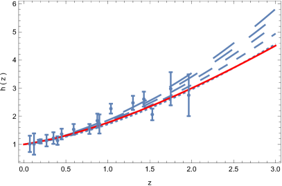
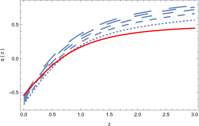
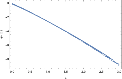
As one can see from Figure 1, for the considered range of parameters, our model can reproduce the observational data of the Hubble function. Moreover, for redshifts $0\leq z<2$, the predictions of the proposed model are in almost exact accordance with those of the standard $\Lambda$CDM paradigm. For $z>2$, there is a small deviation in the values predicted for the Hubble function, our model predicting larger values. Small deviations also appear in the deceleration parameter. It is important to mention that the behaviour of the cosmological parameters depends on the choice of inital condition $\Psi(0)$. Interestingly, this choice does not affect heavily the behaviour of the torsion vector $\Psi(z)$, only at higher redshifts, as can be seen from Figure 2.

Om(z)𝑂𝑚𝑧Om(z) 
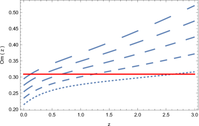
as represented in Figure 2 is very different as compared to the diagnostic function of the ΛΛ\LambdaCDM model, in which Om(z)𝑂𝑚𝑧Om(z) is constant. Our model predicts a positive slope for Om(z)𝑂𝑚𝑧Om(z), which indicates a phantom-like evolution.

Refer to caption
Refer to caption
Figure 1: Variations of the dimensionless Hubble function $h(z)$(left panel), and of the deceleration parameter $q(z)$ (right panel) for the initial conditions $\Psi(0)=-0.06$ (dotted curve), $\Psi(0)=-0.08$ (short dashed curve), $\Psi(0)=-0.10$ (dashed curve) , $\Psi(0)=-0.12$ (long dashed curve) and $\Psi(0)=-0.14$ (ultra long dashed curve), respectively. The observational data for the Hubble function are represented with their error bars, while the red curve depicts the predictions of the $\Lambda$CDM model.
Refer to caption
Refer to caption
Figure 2: Variations of the dimensionless torsion vector $\Psi(z)$ (left panel), and of the $Om(z)$ function (right panel) for the initial conditions $\Psi(0)=-0.06$ (dotted curve), $\Psi(0)=-0.08$ (short dashed curve), $\Psi(0)=-0.10$ (dashed curve) , $\Psi(0)=-0.12$ (long dashed curve) and $\Psi(0)=-0.14$ (ultra long dashed curve), respectively. The red curve represents the predictions of the $\Lambda$CDM model.

5 Summary and Outlook

In the present work, we described a class of affine connection, first considered by Schrödinger, in a coordinate-free manner, providing mathematicians with a basis for further studying their properties. After outlining their basic properties, we gave examples of such connections, realized through either torsion, non-metricity or both, culminating in the definition of three distinct geometries: Weyl-Schrödinger, Yano-Schrödinger and Friedmann-Weyl-Schrödinger. We obtained explicit formulae for the curvature tensors of the aforementioned three connections, with the help of which we provided for the first time in the literature an explicit example of a non-static Einstein-Schrödinger manifold realized by torsion. To demonstrate the applicability of the introduced mathematics, we proposed a geometric generalization of standard general relativity, in which the effects of dark energy have a firm geometric foundation. In contrast to the standard approach, in which these effects are explained by a cosmological constant $\Lambda$, often associated with dark energy, our proposed model explains the observational data using a generalized geometry, in which lengths are preserved, making the geometry physically reasonable.

We would like to point out that our cosmological results are qualitative in nature. To confirm or disprove the validity of Yano-Schrödinger gravity, a detailed analysis using Monte-Carlo methods for a large number of data sets is necessary. Nevertheless, for the data set presented in [40], our model fits well the observational data of the Hubble function.

This work could open several research directions, both in the direction of physics and mathematics. From a physical perspective, it would be interesting to provide actions, which lead to Schrödinger connections, similar to the one provided by Silke and Klemm in [32]. A long standing open problem of mathematical physics was solved in [42], where an action principle for the Einstein-Weyl equations was worked out. As Einstein-Weyl manifolds are simply Einstein manifolds equipped with a Weyl connection, it could be interesting to provide an action principle for Einstein-Schrödinger manifolds with a Weyl-type non-metricity.

From the mathematical perspective, the theory of Schrödinger connections is wide open, as they were not considered in the literature before. We hope that presenting in a geometric, coordinate-free way this class of affine connections, which are physically reasonable, will stern the interest of mathematicians to investigate their mathematical properties in more detail. Historically, this happened for semi-symmetric connections, which were first proposed by Friedmann and Schouten [7], but were largely ignored by mathematicians, until Kentaro Yano’s foundational paper [18], in which he presented the curvature tensors of this connection in a geometric, coordinate-free manner. This paper made the mathematical community more interested in semi-symmetric connections. Since then, researchers have been looking into subspaces that have a semi-symmetric connection. It remains an open question, whether any of the results from semi-symmetric connections could be translated or utilized in the theory of Yano-Schrödinger connections, which are realized by a semi-symmetric type of torsion.

Appendix A Ricci Tensor of Friedmann-Weyl-Schrödinger Geometry

$\displaystyle R_{\mu\nu}=\overset{\circ}{R}_{\mu\nu}$ $\displaystyle+\overset{\circ}{\nabla}_{\alpha}\left(g_{\mu\nu}\pi^{\alpha}-\frac{1}{2}\left(\delta^{\alpha}_{\mu}\pi_{\nu}+\delta^{\alpha}_{\nu}\pi_{\mu}\right)+2W^{\alpha}g_{\mu\nu}+2W_{\nu}\delta^{\alpha}_{\mu}+2W_{\mu}\delta^{\alpha}_{\nu}\right)$
$\displaystyle-\overset{\circ}{\nabla}_{\nu}\left(g_{\mu\alpha}\pi^{\alpha}-\frac{1}{2}\left(\delta^{\alpha}_{\mu}\pi_{\alpha}+\delta^{\alpha}_{\alpha}\pi_{\mu}\right)+2W^{\alpha}g_{\alpha\mu}+2W_{\mu}\delta^{\alpha}_{\alpha}+2W_{\alpha}\delta^{\alpha}_{\mu}\right)$
$\displaystyle+\left(g_{\rho\alpha}\pi^{\alpha}-\frac{1}{2}\left(\delta^{\alpha}_{\rho}\pi_{\alpha}+\delta^{\alpha}_{\alpha}\pi_{\rho}\right)+2W^{\alpha}g_{\alpha\rho}+2W_{\rho}\delta^{\alpha}_{\alpha}+2W_{\alpha}\delta^{\alpha}_{\rho}\right)\times$
$\displaystyle\times\left(g_{\mu\nu}\pi^{\rho}-\frac{1}{2}\left(\delta^{\rho}_{\mu}\pi_{\nu}+\delta^{\rho}_{\nu}\pi_{\mu}\right)+2W^{\rho}g_{\mu\nu}+2W_{\nu}\delta^{\rho}_{\mu}+2W_{\mu}\delta^{\rho}_{\nu}\right)$
$\displaystyle-\left(g_{\rho\nu}\pi^{\alpha}-\frac{1}{2}\left(\delta^{\alpha}_{\rho}\pi_{\nu}+\delta^{\alpha}_{\nu}\pi_{\rho}\right)+2W^{\alpha}g_{\nu\rho}+2W_{\rho}\delta^{\alpha}_{\nu}+2W_{\nu}\delta^{\alpha}_{\rho}\right)\times$
$\displaystyle\times\left(g_{\mu\alpha}\pi^{\rho}-\frac{1}{2}\left(\delta^{\rho}_{\mu}\pi_{\alpha}+\delta^{\rho}_{\alpha}\pi_{\mu}\right)+2W^{\rho}g_{\alpha\mu}+2W_{\mu}\delta^{\rho}_{\alpha}+2W_{\alpha}\delta^{\rho}_{\mu}\right)$
$\displaystyle=\overset{\circ}{R}_{\mu\nu}$ $\displaystyle+g_{\mu\nu}\overset{\circ}{\nabla}_{\alpha}\pi^{\alpha}-\frac{1}{2}\overset{\circ}{\nabla}_{\mu}\pi_{\nu}-{\color[rgb]{1,.5,0}\frac{1}{2}\overset{\circ}{\nabla}_{\nu}\pi_{\mu}}+2g_{\mu\nu}\overset{\circ}{\nabla}_{\alpha}W^{\alpha}+2\overset{\circ}{\nabla}_{\mu}W_{\nu}+{\color[rgb]{0,0,1}2\overset{\circ}{\nabla}_{\nu}W_{\mu}}$
$\displaystyle-{\color[rgb]{1,.5,0}\overset{\circ}{\nabla}_{\nu}\pi_{\mu}}+{\color[rgb]{1,.5,0}\frac{1}{2}\overset{\circ}{\nabla}_{\nu}\pi_{\mu}}+{\color[rgb]{1,.5,0}2\overset{\circ}{\nabla}_{\nu}\pi_{\mu}}-{\color[rgb]{0,0,1}2\overset{\circ}{\nabla}_{\nu}W_{\mu}}-{\color[rgb]{0,0,1}8\overset{\circ}{\nabla}_{\nu}W_{\mu}}-{\color[rgb]{0,0,1}2\overset{\circ}{\nabla}_{\nu}W_{\mu}}$
$\displaystyle+\left(-\frac{3}{2}\pi_{\rho}+12W_{\rho}\right)\times\left(g_{\mu\nu}\pi^{\rho}-\frac{1}{2}\left(\delta^{\rho}_{\mu}\pi_{\nu}+\delta^{\rho}_{\nu}\pi_{\mu}\right)+2W^{\rho}g_{\mu\nu}+2W_{\nu}\delta^{\rho}_{\mu}+2W_{\mu}\delta^{\rho}_{\nu}\right)$
$\displaystyle-{\color[rgb]{1,0,0}\pi_{\nu}\pi_{\mu}}+{\color[rgb]{0,1,1}\frac{1}{2}g_{\mu\nu}\pi^{\alpha}\pi_{\alpha}}+{\color[rgb]{1,0,0}\frac{1}{2}\pi_{\nu}\pi_{\mu}}-{\color[rgb]{1,0,1}2W_{\nu}\pi_{\mu}}-{\color[rgb]{0,0.6,0}2\pi_{\nu}W_{\mu}}-{\color[rgb]{0.45,0.01,0.92}2g_{\mu\nu}\pi^{\alpha}W_{\alpha}}$
$\displaystyle+{\color[rgb]{1,0,0}\frac{1}{2}\pi_{\nu}\pi_{\mu}}-{\color[rgb]{1,0,0}\frac{1}{4}\pi_{\mu}\pi_{\nu}}-{\color[rgb]{1,0,0}\pi_{\nu}\pi_{\mu}}+{\color[rgb]{0,0.6,0}\pi_{\nu}W_{\mu}}+{\color[rgb]{0,0.6,0}4\pi_{\nu}W_{\mu}}+{\color[rgb]{0,0.6,0}W_{\mu}\pi_{\nu}}$
$\displaystyle+{\color[rgb]{0,1,1}\frac{1}{2}g_{\mu\nu}\pi_{\rho}\pi^{\rho}}-{\color[rgb]{1,0,0}\frac{1}{4}\pi_{\nu}\pi_{\mu}}-{\color[rgb]{1,0,0}\frac{1}{4}\pi_{\nu}\pi_{\mu}}+{\color[rgb]{0.45,0.01,0.92}g_{\mu\nu}\pi_{\rho}W^{\rho}}+{\color[rgb]{0,0.6,0}\pi_{\nu}W_{\mu}}+{\color[rgb]{1,0,1}W_{\nu}\pi_{\mu}}$
$\displaystyle-{\color[rgb]{0,0.6,0}2W_{\mu}\pi_{\nu}}+{\color[rgb]{0.45,0.01,0.92}W^{\alpha}\pi_{\alpha}g_{\mu\nu}}+{\color[rgb]{1,0,1}W_{\nu}\pi_{\mu}}-{\color[rgb]{0.0600000000000001,0.46,1}4W_{\mu}W_{\nu}}-{\color[rgb]{0.0600000000000001,0.46,1}4W_{\nu}W_{\mu}}-{\color[rgb]{0.4,0,0}4W^{\alpha}W_{\alpha}g_{\mu\nu}}$
$\displaystyle-{\color[rgb]{0.45,0.01,0.92}2g_{\mu\nu}W_{\rho}\pi^{\rho}}+{\color[rgb]{0,0.6,0}W_{\mu}\pi_{\nu}}+{\color[rgb]{1,0,1}W_{\nu}\pi_{\mu}}-{\color[rgb]{0.4,0,0}4W_{\rho}W^{\rho}g_{\mu\nu}}-{\color[rgb]{0.0600000000000001,0.46,1}4W_{\nu}W_{\mu}}-{\color[rgb]{0.0600000000000001,0.46,1}4W_{\mu}W_{\nu}}$
$\displaystyle-{\color[rgb]{1,0,1}2W_{\nu}\pi_{\mu}}+{\color[rgb]{1,0,1}W_{\nu}\pi_{\mu}}+{\color[rgb]{1,0,1}4W_{\nu}\pi_{\mu}}-{\color[rgb]{0.0600000000000001,0.46,1}4W_{\nu}W_{\mu}}-{\color[rgb]{0.0600000000000001,0.46,1}16W_{\nu}W_{\mu}}-{\color[rgb]{0.0600000000000001,0.46,1}4W_{\mu}W_{\nu}}$
$\displaystyle=\overset{\circ}{R}_{\mu\nu}$ $\displaystyle+g_{\mu\nu}\overset{\circ}{\nabla}_{\alpha}\pi^{\alpha}-\frac{1}{2}\overset{\circ}{\nabla}_{\mu}\pi_{\nu}+{\color[rgb]{1,.5,0}\overset{\circ}{\nabla}_{\nu}\pi_{\mu}}+2g_{\mu\nu}\overset{\circ}{\nabla}_{\alpha}W^{\alpha}+2\overset{\circ}{\nabla}_{\mu}W_{\nu}-{\color[rgb]{0,0,1}10\overset{\circ}{\nabla}_{\nu}W_{\mu}}$
$\displaystyle-\frac{3}{2}g_{\mu\nu}\pi_{\rho}\pi^{\rho}+\frac{3}{4}\pi_{\mu}\pi_{\nu}+\frac{3}{4}\pi_{\nu}\pi_{\mu}-3g_{\mu\nu}\pi_{\rho}W^{\rho}-3\pi_{\mu}W_{\nu}-3\pi_{\nu}W_{\mu}$
$\displaystyle+12g_{\mu\nu}W_{\rho}\pi^{\rho}-6W_{\mu}\pi_{\nu}-6W_{\nu}\pi_{\mu}+24g_{\mu\nu}W^{\rho}W_{\rho}+24W_{\mu}W_{\nu}+24W_{\nu}W_{\mu}$
$\displaystyle-{\color[rgb]{1,0,0}\frac{7}{4}\pi_{\nu}\pi_{\mu}}+{\color[rgb]{0,1,1}g_{\mu\nu}\pi_{\rho}\pi^{\rho}}+{\color[rgb]{1,0,1}4W_{\nu}\pi_{\mu}}+{\color[rgb]{0,0.6,0}4\pi_{\nu}W_{\mu}}-{\color[rgb]{0.45,0.01,0.92}2g_{\mu\nu}W_{\rho}\pi^{\rho}}-{\color[rgb]{0.0600000000000001,0.46,1}40W_{\nu}W_{\mu}}-{\color[rgb]{0.4,0,0}8W_{\rho}W^{\rho}g_{\mu\nu}}$
$\displaystyle=\overset{\circ}{R}_{\mu\nu}$ $\displaystyle+g_{\mu\nu}\overset{\circ}{\nabla}_{\alpha}\pi^{\alpha}-\frac{1}{2}\overset{\circ}{\nabla}_{\mu}\pi_{\nu}+\overset{\circ}{\nabla}_{\nu}\pi_{\mu}-\frac{1}{2}g_{\mu\nu}\pi^{\rho}\pi_{\rho}-\frac{1}{4}\pi_{\nu}\pi_{\mu}$
$\displaystyle+2g_{\mu\nu}\overset{\circ}{\nabla}_{\alpha}W^{\alpha}+2\overset{\circ}{\nabla}_{\mu}W_{\nu}-10\overset{\circ}{\nabla}_{\nu}W_{\mu}+16W_{\rho}W^{\rho}g_{\mu\nu}+8W_{\nu}W_{\mu}$
$\displaystyle+7g_{\mu\nu}\pi_{\rho}W^{\rho}-5\pi_{\mu}W_{\nu}-5\pi_{\nu}W_{\mu}.$

Appendix B Derivation of Friedmann Equations

In this appendix we derive the generalized Friedmann equations in Schrödinger-Yano gravity, using the assumptions from section 4.1. As a starting point, recall that in the standard Riemannian geometry for the Levi-Civita connection the components of the Ricci tensor are given by

$$\overset{\circ}{R}_{00}=-3\frac{\ddot{a}}{a},\;\;\overset{\circ}{R}_{11}=\overset{\circ}{R}_{22}=\overset{\circ}{R}_{33}=a\ddot{a}+2\dot{a}^{2}.$$ (B.1)

The Ricci scalar takes the well-known form

$$\overset{\circ}{R}=6\left(\frac{\ddot{a}}{a}+\frac{\dot{a}^{2}}{a^{2}}\right),$$ (B.2)

while the non-vanishing Christoffel symbols read

$$\tensor{\gamma}{{}^{0}_{i}{}_{j}}=a\dot{a}\delta_{ij},$$ (B.3)
$$\tensor{\gamma}{{}^{i}_{0}{}_{j}}=\frac{\dot{a}}{a}\delta^{i}_{j},\;\;i,j=1,2,3.$$ (B.4)

The generalized Einstein equation (4.3) in the $00$ component takes the form

$$\overset{\circ}{R}_{00}-\frac{1}{2}g_{00}\overset{\circ}{R}-\frac{5}{4}g_{00}\overset{\circ}{\nabla}_{\alpha}\pi^{\alpha}+\frac{1}{4}\left(\overset{\circ}{\nabla}_{0}\pi_{0}+\overset{\circ}{\nabla}_{0}\pi_{0}\right)+\frac{5}{8}g_{00}\pi^{\alpha}\pi_{\alpha}-\frac{1}{4}\pi_{0}\pi_{0}=8\pi T_{00}$$ (B.5)

Before evaluating the above equation, we will compute some terms that appear explicitly. With our assumptions, we have

$$\pi_{0}=\psi,\;\;\pi^{0}=-\psi,\;\;T_{00}=\rho,$$ (B.6)

from which we get

$$\overset{\circ}{\nabla}_{0}\pi_{0}=\dot{\psi}.$$ (B.7)

The covariant divergence of $\pi$ is given by

$$\overset{\circ}{\nabla}_{\alpha}\pi^{\alpha}=-\dot{\psi}-3\frac{\dot{a}}{a}\psi.$$ (B.8)

Substituting everything back into (B.5) we obtain

$$-3\frac{\ddot{a}}{a}+\frac{1}{2}6\left(\frac{\ddot{a}}{a}+\frac{\dot{a}^{2}}{a^{2}}\right)+\frac{5}{4}\left(-\dot{\psi}-3\frac{\dot{a}}{a}\psi\right)+\frac{1}{4}\left(2\dot{\psi}\right)+\frac{5}{8}\psi^{2}-\frac{1}{4}\psi^{2}=8\pi\rho.$$ (B.9)

A straightforward algebraic simplification leads to

$$3\frac{\dot{a}^{2}}{a^{2}}-\frac{3}{4}\dot{\psi}-\frac{15}{4}\frac{\dot{a}}{a}\psi+\frac{3}{8}\psi^{2}=8\pi\rho.$$ (B.10)

By introducing the Hubble function $H=\frac{\dot{a}}{a}$, we have the first Friedmann equation

$$3H^{2}=8\pi\rho+\frac{3}{4}\dot{\psi}+\frac{15}{4}H\psi-\frac{3}{8}\psi^{2}.$$ (B.11)

For the second Friedmann equation, we consider the $ii$ components of the Einstein equation (4.3)

$$\overset{\circ}{R}_{ii}-\frac{1}{2}g_{ii}\overset{\circ}{R}-\frac{5}{4}g_{ii}\overset{\circ}{\nabla}_{\alpha}\pi^{\alpha}+\frac{1}{4}\left(\overset{\circ}{\nabla}_{i}\pi_{i}+\overset{\circ}{\nabla}_{i}\pi_{i}\right)+\frac{5}{8}g_{ii}\pi^{\alpha}\pi_{\alpha}-\frac{1}{4}\pi_{i}\pi_{i}=8\pi T_{ii}.$$ (B.12)

Thanks to the symmetry the equations will take the same form for all spatial indices $i$. For simplicity, we consider $i=1$. From our conventions, it can be seen that

$$\pi_{1}=0,\;\;T_{11}=pa^{2}.$$ (B.13)

So for the Einstein equation in the $11$ component we have

$$a\ddot{a}+2\dot{a}^{2}-a^{2}\frac{1}{2}6\left(\frac{\ddot{a}}{a}+\frac{\dot{a}^{2}}{a^{2}}\right)-\frac{5}{4}a^{2}\left(-\dot{\psi}-3\frac{\dot{a}}{a}\psi\right)+\frac{1}{4}\left(2(-a\dot{a}\psi)\right)-\frac{5}{8}a^{2}\psi^{2}=8\pi pa^{2}.$$ (B.14)

Multiplying the terms out yields

$$a\ddot{a}+2\dot{a}^{2}-3a\ddot{a}-3\dot{a}^{2}+\frac{5}{4}a^{2}\dot{\psi}+\frac{15}{4}a\dot{a}\psi-\frac{1}{2}a\dot{a}\psi-\frac{5}{8}a^{2}\psi^{2}=8\pi pa^{2}.$$ (B.15)

Collecting the terms and dividing by $a^{2}$ results in

$$-2\frac{\ddot{a}}{a}-\frac{\dot{a}^{2}}{a^{2}}+\frac{5}{4}\dot{\psi}+\frac{13}{4}\frac{\dot{a}}{a}\psi-\frac{5}{8}\psi^{2}=8\pi p,$$ (B.16)

which can be equivalently rewritten as

$$-2\dot{H}-2H^{2}-H^{2}+\frac{5}{4}\dot{\psi}+\frac{13}{4}H\psi-\frac{5}{8}\psi^{2}=8\pi p.$$ (B.17)

Thus the final form of the second Friedmann equation is obtained

$$3H^{2}+2\dot{H}=-8\pi p+\frac{5}{4}\dot{\psi}+\frac{13}{4}H\psi-\frac{5}{8}\psi^{2}.$$ (B.18)

Acknowledgments

The author would like to thank Collegium Talentum Hungary and the StarUBB institute, for the research scholarships provided. Discussions with Prof. Tiberiu Harko and Tudor Patuleanu are highly appreciated.

References

  • [1] H. Weyl In Sitzungsberichte der Königlich Preussischen Akademie der Wissenschaften zu Berlin, 1918, pp. 465
  • [2] É. Cartan In Comptes Rendus de l’Académie des Sciences (Paris) 174, 1922, pp. 593
  • [3] É. Cartan In Annales de l’École Normale Supérieure 40, 1923, pp. 325
  • [4] É. Cartan In Annales de l’École Normale Supérieure 41, 1924, pp. 1
  • [5] É. Cartan In Annales de l’École Normale Supérieure 42, 1925, pp. 17
  • [6] H..M. Goenner “On the History of Unified Field Theories” In Living Reviews in Relativity 7, 2004
  • [7] A. Friedmann and J.A. Schouten “Über die Geometrie der halbsymmetrischen Übertragung” In Mathematische Zeitschrift 21, 1924, pp. 211–223
  • [8] Gh. Fasihi-Ramandi “Semi-Symmetric connection formalism for unification of gravity and electromagnetism” In Journal of Geometry and Physics 144, 2019, pp. 245–250
  • [9] E. Zangiabadi and Z. Nazari “Semi-Riemannian manifold with semi-symmetric connections” In Journal of Geometry and Physics 169, 2021, pp. 104341
  • [10] J.A. Schouten “Ricci Calculus, An Introduction to Tensor Analysis and Geometrical Applications” Berlin-Göttingen-Heidelberg: Springer-Verlag, 1954
  • [11] B. Barua and A.K. Ray “Some properties of semisymmetric metric connection in a Riemannian manifold” In Indian Journal of Pure and Applied Mathematics 16, 1985, pp. 736–740
  • [12] U.C. De and S.C. Biswas “On a type of semi-symmetric metric connection on a Riemannian manifold” In Publications de l’Institut Mathématique (Beograd) 61, 1997, pp. 90–96
  • [13] T. Imai “Notes on semi-symmetric metric connections” In Tensor, New Series 24, 1972, pp. 293–296
  • [14] N.S. Agashe and M.R. Chafle “A semi-symmetric non-metric connection on a Riemannian manifold” In Indian Journal of Pure and Applied Mathematics 23, 1992, pp. 399–409
  • [15] K. Amur and S.S. Pujar “On submanifolds of a Riemannian manifold admitting a metric semi-symmetric connection” In Tensor 32, 1978, pp. 35–38
  • [16] S. Sharfuddin and S.I. Husain “Semi-symmetric metric connections in almost contact manifolds” In Tensor 30, 1976, pp. 133–139
  • [17] Ibrahim Al-Dayel and Meraj Ali Khan “Impact of Semi-Symmetric Metric Connection On Homology of Warped Product Pointwise Semi-Slant Submanifolds of an Odd-Dimensional Sphere” In Symmetry 15.8, 2023, pp. 1606
  • [18] K. Yano “On Semi-Symmetric Metric Connection” In Revue Roumaine de Mathématique Pures et Appliquées 15, 1970, pp. 1579–1586
  • [19] J.T. Wheeler “Weyl Geometry” In General Relativity and Gravitation 50.7, 2018, pp. 80
  • [20] F. London “Quantum Mechanical interpretation of the Weyl theory” In Zeitschrift für Physik 42, 1927, pp. 375
  • [21] L.’ Raifeartaigh “The Dawning of Gauge Theory” Princeton, NJ: Princeton University Press, 1997, pp. 249
  • [22] D.. Ghilencea “Gauging scale symmetry and inflation: Weyl versus Palatini gravity” In European Physical Journal C 81, 2021, pp. 510
  • [23] D.. Ghilencea “Standard Model in Weyl conformal geometry” In European Physical Journal C 82, 2022, pp. 23
  • [24] D.. Ghilencea “Non-metric geometry as the origin of mass in gauge theories of scale invariance” In European Physical Journal C 83, 2023, pp. 176
  • [25] M. Weisswange, D.. Ghilencea and D. Stöckinger “Quantum scale invariance in gauge theories and applications to muon production” In Physical Review D 107, 2023, pp. 085008
  • [26] D.. Ghilencea and C.. Hill “Renormalization group for nonminimal $\phi^{2}R$ couplings and gravitational contact interactions” In Physical Review D 107, 2023, pp. 085013
  • [27] J.-Z. Yang, S. Shahidi and T. Harko “Black hole solutions in the quadratic Weyl conformal geometric theory of gravity” In European Physical Journal C 82, 2022, pp. 1171
  • [28] P. Burikham, T. Harko, K. Pimsamarn and S. Shahidi “Dark matter as a Weyl geometric effect” In Physical Review D 107, 2023, pp. 064008
  • [29] M. Craciun and T. Harko “Testing Weyl geometric gravity with the SPARC galactic rotation curves database” To be published in 2024 In Physics of the Dark Universe
  • [30] T. Harko and S. Shahidi “Coupling matter and curvature in Weyl geometry: conformally invariant $f(R,L_{m})$ gravity” In European Physical Journal C 82, 2022, pp. 219
  • [31] T. Harko and S. Shahidi “Palatini formulation of the conformally invariant $f(R,L_{m})$ gravity theory” In European Physical Journal C 82, 2022, pp. 1003
  • [32] Silke Klemm and Lucrezia Ravera In Physics Letters B 817, 2021, pp. 136291
  • [33] Lei Ming, Shi-Dong Liang, Hong-Hao Zhang and Tiberiu Harko In Physical Review D 109, 2024, pp. 024003
  • [34] E. Schrödinger “Space-time Structure” Cambridge University Press, 1954
  • [35] A. Besse “Einstein Manifolds” Springer-Verlag Berlin Heidelberg New York, 1987
  • [36] Silke Klemm and Lucrezia Ravera “Einstein manifolds with torsion and nonmetricity” In Physical Review D 101, 2020, pp. 044011
  • [37] Lionel Mason “The Einstein-Weyl equations, scattering maps, and holomorphic disks” In Mathematical Research Letters 16, 2009, pp. 291–301
  • [38] Mustafa Deniz Turkoglu “Geometry of Weyl Spaces with a Special Connection” PhD thesis
  • [39] Y. al. “Planck 2018 results. I. Overview and the cosmological legacy of Planck” In Astronomy and Astrophysics 641, 2020, pp. A1
  • [40] H. Boumaza and K. Nouicer “Growth of matter perturbations in the bi-Galileons field model” In Physical Review D 100, 2019, pp. 124047
  • [41] V. Sahni, A. Shafieloo and A.. Starobinsky “Two new diagnostics of dark energy” In Physical Review D 78, 2008, pp. 103502
  • [42] Silke Klemm and Lucrezia Ravera In Journal of Geometry and Physics 158, 2020, pp. 103958