Improved Evidential Deep Learning via a Mixture of Dirichlet Distributions

Abstract

This paper explores a modern predictive uncertainty estimation approach, called evidential deep learning (EDL), in which a single neural network model is trained to learn a meta distribution over the predictive distribution by minimizing a specific objective function. Despite their strong empirical performance, recent studies by Bengs et al. identify a fundamental pitfall of the existing methods: the learned epistemic uncertainty may not vanish even in the infinite-sample limit. We corroborate the observation by providing a unifying view of a class of widely used objectives from the literature. Our analysis reveals that the EDL methods essentially train a meta distribution by minimizing a certain divergence measure between the distribution and a sample-size-independent target distribution, resulting in spurious epistemic uncertainty. Grounded in theoretical principles, we propose learning a consistent target distribution by modeling it with a mixture of Dirichlet distributions and learning via variational inference. Afterward, a final meta distribution model distills the learned uncertainty from the target model. Experimental results across various uncertainty-based downstream tasks demonstrate the superiority of our proposed method, and illustrate the practical implications arising from the consistency and inconsistency of learned epistemic uncertainty.

1 Introduction

Uncertainty quantification (UQ) has become an increasingly important task for building trustworthy machine learning systems. Accurate estimation of uncertainty in the prediction is crucial to enhance the reliability of a predictive model, especially for high-stake applications such as medical diagnosis (Begoli et al., 2019; Djulbegovic et al., 2011). For a high-level overview on the fast-moving field, we refer a reader to comprehensive survey papers (Abdar et al., 2021; Gawlikowski et al., 2021).

Many UQ approaches adopt a Bayesian perspective and leverage a posterior distribution over model parameters to capture uncertainty. Several approaches have been proposed for operationalizing Bayesian variants of neural networks (Neal, 2012; Blundell et al., 2015; Sato & Nakagawa, 2014). Others use ensembles (Lakshminarayanan et al., 2017) or Monte Carlo dropout (Gal & Ghahramani, 2016), to capture predictive uncertainties. These approaches, however, often suffer from expensive computational costs, as they involve training, storing, and running multiple models.

More recently, researchers have proposed evidential deep learning (EDL) in which a single neural network and a single forward pass through the network is used to estimate the uncertainty of a prediction at a given point; see, e.g., a recent survey paper (Ulmer et al., 2023). The core idea is to learn a model mapping input data to the parameters of a meta distribution, which is a distribution over the predictive distribution. For example, in classification, the model parameterizes a Dirichlet distribution to represent the distribution of a categorical distribution over possible labels. Such a meta distribution effectively captures various types of uncertainties: i.e., the epistemic uncertainty and aleatoric uncertainty can be represented by the spread and mean of the output Dirichlet distribution, respectively.

Despite the promising performance of existing EDL methods in various downstream tasks, such as out-of-distribution (OOD) detection, theoretical understanding on the learned uncertainty from this type of UQ model has been lacking. Recently, Bengs et al. (2022) identified a fundamental issue with the learned uncertainties from this approach—the learned epistemic uncertainty does not vanish even in the asymptotic limit of infinite training samples. This can lead to inflated uncertainties and undesirable downstream outcomes in the finite-sample scenarios encountered in practice.

This paper aims to fill the fundamental gap between the theory and practice in the EDL approach. As a theoretical investigation, in a spirit similar to (Bengs et al., 2022), we provide a complementary, yet unifying perspective on the existing EDL approaches proposed in the literature. We provide a sharper characterization of the optimal meta distribution defined by a wide class of the existing methods, and reveal that existing methods train the meta distribution to fit a sample-size-independent target distribution. We empirically demonstrate that this leads to spurious epistemic uncertainty that does not vanish in the infinite-sample limit. Fig. 1 illustrates the behavior; see Sec. 3 for the details.

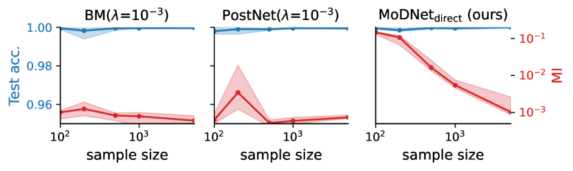
Figure 1: Epistemic uncertainty and test accuracy v.s. number of training data. Existing methods (Belief Matching (BM) (Joo et al., 2020) and Posterior Network (PostNet) (Charpentier et al., 2020)) learn spurious epistemic uncertainty. Our method (ModNet) learns epistemic uncertainty that monotonically vanishes with more data, as shown in the last column; see Sec. 3.3 for the details.

Building upon the insight, we provide a practical solution by constructing a target distribution that allows for the epistemic uncertainty to shrink with increasing training samples. We propose a new latent variable model based on a mixture of Dirichlet distributions and employ variational inference for approximating the posterior distribution. The resulting posterior predictive meta distribution becomes peakier with more training data, exhibiting the naturally diminishing behavior in epistemic uncertainty for in-distribution data. Hence, finally, we propose to use an auxiliary UQ model to distill the posterior-predictive meta distribution, leading to the desired behavior in epistemic uncertainty as well as efficient test-time performance and better OOD generalization. We empirically validate our theory and demonstrate the superiority of our proposed method in the UQ downstream tasks as well as the consequence of the well-behaved epistemic uncertainty.

Summary of contributions. In this paper, we aim to clarify and address the common issue of the learned epistemic uncertainty in the EDL approach by providing the following insights: (1) we offer a sharper theoretical analysis than (Bengs et al., 2022) on the behavior of the existing EDL methods by unifying several representative objective functions; (2) we empirically demonstrate the issue in the learned epistemic uncertainty with real-data experiments; (3) we propose a novel method that can effectively mitigate the issue towards more reliable Uncertainty Quantification (UQ). To the best of our knowledge, this is the first attempt to address and rectify the issue in the literature.

2 Preliminaries

In this paper, we focus on the classification problem: we wish to learn an underlying distribution $p(x,y)$ over $\mathcal{X}\times\mathcal{Y}$ from data $\mathcal{D}=\{(x_{i},y_{i})\}_{i=1}^{N}$ drawn from an underlying data distribution $p(x,y)$, where $\mathcal{Y}\mathrel{\mathop{\mathchar 58\relax missing}}=[C]\mathrel{\mathop{\mathchar 58\relax missing}}=\{1,\ldots,C\}$ is a discrete label set. In addition to accurately learning the conditional distribution $\eta_{y}(x)\mathrel{\mathop{\mathchar 58\relax missing}}=p(y\mathchoice{\mspace{1.0mu}|\mspace{1.0mu}}{|}{|}{|}x)$, we wish to quantify “uncertainty” of the learned probabilistic classifier.

Arguably, the most widely studied UQ approach is the Bayesian approach, in which a parametric classifier $p(y\mathchoice{\mspace{1.0mu}|\mspace{1.0mu}}{|}{|}{|}x,\psi)$ is trained via Bayesian principle, and inference is performed with the predictive posterior distribution $p(y\mathchoice{\mspace{1.0mu}|\mspace{1.0mu}}{|}{|}{|}x,\mathcal{D})\mathrel{\mathop{\mathchar 58\relax missing}}=\int p(y\mathchoice{\mspace{1.0mu}|\mspace{1.0mu}}{|}{|}{|}x,\psi)p(\psi\mathchoice{\mspace{1.0mu}|\mspace{1.0mu}}{|}{|}{|}\mathcal{D})\mathop{}\!\mathrm{d}\psi$, where $p(\psi\mathchoice{\mspace{1.0mu}|\mspace{1.0mu}}{|}{|}{|}\mathcal{D})$ is the model posterior distribution. As alluded to earlier, the Bayesian approach is computationally demanding due to the intractability of $p(\psi\mathchoice{\mspace{1.0mu}|\mspace{1.0mu}}{|}{|}{|}\mathcal{D})$ and the need for computing the integration over $\psi$. We thus focus on the EDL approach, where it is common to assume the best single model $\psi^{\star}$ with data $\mathcal{D}$, without the Bayesian inference (Ulmer et al., 2023).

2.1 Evidential Deep Learning

The EDL approach is based on further decomposing the probabilistic classifier $p_{\psi}(y\mathchoice{\mspace{1.0mu}|\mspace{1.0mu}}{|}{|}{|}x)\mathrel{\mathop{\mathchar 58\relax missing}}=p(y\mathchoice{\mspace{1.0mu}|\mspace{1.0mu}}{|}{|}{|}x,\psi)$ as $p_{\psi}(y\mathchoice{\mspace{1.0mu}|\mspace{1.0mu}}{|}{|}{|}x)=\int_{\Delta^{C-1}}p_{\psi}(\boldsymbol{\pi}\mathchoice{\mspace{1.0mu}|\mspace{1.0mu}}{|}{|}{|}x)p(y\mathchoice{\mspace{1.0mu}|\mspace{1.0mu}}{|}{|}{|}\boldsymbol{\pi})\mathop{}\!\mathrm{d}\boldsymbol{\pi}$, where a probability vector $\boldsymbol{\pi}\in\Delta^{C-1}$ is the categorical distribution over $C$ classes, $p(y\mathchoice{\mspace{1.0mu}|\mspace{1.0mu}}{|}{|}{|}\boldsymbol{\pi})\mathrel{\mathop{\mathchar 58\relax missing}}=\pi_{y}$ denotes the categorical likelihood model, and the meta distribution $p_{\psi}(\boldsymbol{\pi}\mathchoice{\mspace{1.0mu}|\mspace{1.0mu}}{|}{|}{|}x)$ is a distribution over the probability simplex $\Delta^{C-1}$, which is thus sometimes called a second-order distribution (Bengs et al., 2022). In this paper, we call it a local UQ model, as it quantifies an uncertainty of prediction for each point locally. This decomposition can be formally understood as assuming that a label $y$ is generated for each $x$ based on the generative model $p_{\psi}(\boldsymbol{\pi}\mathchoice{\mspace{1.0mu}|\mspace{1.0mu}}{|}{|}{|}x)p(y\mathchoice{\mspace{1.0mu}|\mspace{1.0mu}}{|}{|}{|}\boldsymbol{\pi})$; see Fig. 2 for its schematic illustration.

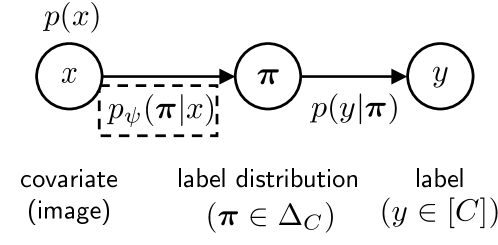
Figure 2: Graphical illustration of the standard EDL model.

For classification, it is common to parameterize the meta distribution $p_{\psi}(\boldsymbol{\pi}\mathchoice{\mspace{1.0mu}|\mspace{1.0mu}}{|}{|}{|}x)$ by the Dirichlet distribution $\mathsf{Dir}(\boldsymbol{\pi};\boldsymbol{\alpha}_{\psi}(x))$ mainly due to its computational tractability from the conjugacy to the categorical likelihood model. Here, each point $x$ has an associated concentration parameter $\boldsymbol{\alpha}_{\psi}(x)\in\mathbb{R}_{\geq 0}^{C}$. We expect $\boldsymbol{\alpha}_{\psi}(x)$ to capture the amount of certainty for the prediction made by the model at a query point $x$. The induced predictive label distribution is then

$$p_{\psi}(y\mathchoice{\mspace{1.0mu}|\mspace{1.0mu}}{|}{|}{|}x)\mathrel{\mathop{\mathchar 58\relax missing}}=\int p_{\psi}(\boldsymbol{\pi}\mathchoice{\mspace{1.0mu}|\mspace{1.0mu}}{|}{|}{|}x)p(y\mathchoice{\mspace{1.0mu}|\mspace{1.0mu}}{|}{|}{|}\boldsymbol{\pi})\mathop{}\!\mathrm{d}\boldsymbol{\pi}=\frac{\alpha_{\psi,y}(x)}{\sum_{y^{\prime}=1}^{C}\alpha_{\psi,y^{\prime}}(x)}.$$

If we parameterize $\boldsymbol{\alpha}_{\psi}(x)$ as $\alpha_{\psi,y}(x)=\exp({\mathbf{w}}_{y}^{\intercal}{\bf f}_{\phi}(x))$ for each $y\in[C]$ with some function $f_{\phi}$ and weight vectors $\mathbf{w}_{1},\ldots,\mathbf{w}_{C}$, it becomes equivalent to the standard softmax parameterization. If we simply train $\psi$ with the standard maximum likelihood objective $D(p(x,y)~{}\|~{}p(x)p_{\psi}(y\mathchoice{\mspace{1.0mu}|\mspace{1.0mu}}{|}{|}{|}x))$, it makes no difference from the standard softmax-based learning. Hence, different optimization objectives are needed for training the meta distribution $p_{\psi}(\boldsymbol{\pi}\mathchoice{\mspace{1.0mu}|\mspace{1.0mu}}{|}{|}{|}x)$.

2.2 Existing EDL Methods: Overview

The different methods in the EDL approach assume a different parametric form of the UQ model and distinct learning criteria. We remark that a recent survey paper (Ulmer et al., 2023) overviews several different methods in the EDL literature, partitioning the literature into prior-network (PriorNet) type methods (Malinin & Gales, 2018, 2019) and posterior-network (PostNet) type methods (Chen et al., 2018; Joo et al., 2020; Charpentier et al., 2020, 2022; Shen et al., 2023). We find, however, the dichotomy rather unnatural, as we show in the next section, the widely adopted PriorNet and PostNet type objectives are exactly equivalent, in sharp contrast to the common understanding.

The distinguishing feature in the PriorNet and PostNet is then the parametric form of $\boldsymbol{\alpha}_{\psi}(x)$. In earlier works such as (Chen et al., 2018; Malinin & Gales, 2018, 2019; Joo et al., 2020), $\boldsymbol{\alpha}_{\psi}(x)$ is typically parameterized by a direct output of a neural network; we call this direct parametrization. Later, Charpentier et al. (2020) brought up a potential issue with the direct parametrization that $\boldsymbol{\alpha}_{\psi}(x)$ can potentially take arbitrary values on the unseen (i.e., out-of-distribution, or OOD) data points. They proposed a more sophisticated parameterization of the form $\boldsymbol{\alpha}_{\psi}(x)\leftarrow\boldsymbol{\alpha}_{0}+\mathbf{N}_{\psi}(x)$, where, for $y\in[C]$, $(\mathbf{N}_{\psi}(x))_{y}\mathrel{\mathop{\mathchar 58\relax missing}}=N\hat{p}(y)p_{\psi_{2}}(f_{\psi_{1}}(x)\mathchoice{\mspace{1.0mu}|\mspace{1.0mu}}{|}{|}{|}y)$, $\hat{p}(y)\mathrel{\mathop{\mathchar 58\relax missing}}=N_{y}/N$, $N_{y}$ denotes the number of data points with label $y$, $N\mathrel{\mathop{\mathchar 58\relax missing}}=\sum_{y\in[C]}N_{y}$, $x\mapsto f_{\psi_{1}}(x)$ a feature extractor, and $p_{\psi_{2}}(z\mathchoice{\mspace{1.0mu}|\mspace{1.0mu}}{|}{|}{|}y)$ a tractable density model such as normalizing flows (Kobyzev et al., 2020) for each $y\in[C]$. The rationale behind the parameterization is twofold. First, it explicitly resembles the posterior distribution update of the Dirichlet distribution, explicitly forcing $\boldsymbol{\alpha}_{\psi}(x)$ to have large values as $N\to\infty$. Second, it explicitly forces the uncertainty has finite constrained budget, i.e., $\int_{\mathcal{X}}\mathds{1}_{C}^{\intercal}\mathbf{N}_{\psi}(x)\mathop{}\!\mathrm{d}x=N$, so that the $\boldsymbol{\alpha}_{\psi}(x)$ cannot output high values for OOD data. We call this density parameterization.

2.3 Definition of Uncertainty and Its Measures

In EDL, the uncertainty captured by $p_{\psi}(\boldsymbol{\pi}\mathchoice{\mspace{1.0mu}|\mspace{1.0mu}}{|}{|}{|}x)$ and $p_{\psi}(y\mathchoice{\mspace{1.0mu}|\mspace{1.0mu}}{|}{|}{|}x)$ are called the epistemic uncertainty and aleatoric (data) uncertainty, respectively. Epistemic uncertainty captures the model’s lack of knowledge arising from the mismatch in the training distribution and test distribution. That is, the distribution $p_{\psi}(\boldsymbol{\pi}\mathchoice{\mspace{1.0mu}|\mspace{1.0mu}}{|}{|}{|}x_{0})$ should be dispersed if the model is uncertain on the particular query point $x_{0}$, and sharp otherwise. As the adjective epistemic suggests, this uncertainty is supposed to vanish at points in the support of the underlying distribution, when the model has observed infinitely many samples. In contrast, the aleatoric uncertainty captures the inherent uncertainty in $p(y\mathchoice{\mspace{1.0mu}|\mspace{1.0mu}}{|}{|}{|}x)$, and thus must be invariant to the sample size in principle.

We consider two standard metrics to measure epistemic uncertainty: (1) differential entropy (DEnt) $h_{\psi}(\boldsymbol{\pi}\mathchoice{\mspace{1.0mu}|\mspace{1.0mu}}{|}{|}{|}x)\mathrel{\mathop{\mathchar 58\relax missing}}=-\int p_{\psi}(\boldsymbol{\pi}\mathchoice{\mspace{1.0mu}|\mspace{1.0mu}}{|}{|}{|}x)\log p_{\psi}(\boldsymbol{\pi}\mathchoice{\mspace{1.0mu}|\mspace{1.0mu}}{|}{|}{|}x)d\boldsymbol{\pi}$; (2) mutual information (MI) $I_{\psi}(y;\boldsymbol{\pi}\mathchoice{\mspace{1.0mu}|\mspace{1.0mu}}{|}{|}{|}x)\mathrel{\mathop{\mathchar 58\relax missing}}=h_{\psi}(\boldsymbol{\pi}\mathchoice{\mspace{1.0mu}|\mspace{1.0mu}}{|}{|}{|}x)-\operatorname{\mathsf{E}}_{p(y\mathchoice{\mspace{1.0mu}|\mspace{1.0mu}}{|}{|}{|}\boldsymbol{\pi})}[h_{\psi}(\boldsymbol{\pi}\mathchoice{\mspace{1.0mu}|\mspace{1.0mu}}{|}{|}{|}x,y)]$. The resulting probabilistic classifier $p_{\psi}(y\mathchoice{\mspace{1.0mu}|\mspace{1.0mu}}{|}{|}{|}x)$ captures both epistemic and aleatoric uncertainties without distinction, and the total uncertainty is often measured via two standard metrics: (1) entropy (Ent) of $p_{\psi}(y\mathchoice{\mspace{1.0mu}|\mspace{1.0mu}}{|}{|}{|}x)$, i.e., $H\left(p_{\psi}(y\mathchoice{\mspace{1.0mu}|\mspace{1.0mu}}{|}{|}{|}x)\right)$; (2) max probability (MaxP) of $p_{\psi}(y\mathchoice{\mspace{1.0mu}|\mspace{1.0mu}}{|}{|}{|}x)$, i.e., $\max_{y}p_{\psi}(y\mathchoice{\mspace{1.0mu}|\mspace{1.0mu}}{|}{|}{|}x)$.

Before we proceed, we remark that there are conflicting definitions of epistemic uncertainty in the literature. On the one hand, earlier works in the classical Bayesian approach defined the uncertainty in the Bayesian posterior $p(\psi\mathchoice{\mspace{1.0mu}|\mspace{1.0mu}}{|}{|}{|}\mathcal{D})$ (Gal et al., 2016; Hüllermeier & Waegeman, 2021) as epistemic uncertainty, which is thus also referred to as model uncertainty. On the other hand, most methods in the EDL approach follow the convention in our paper, which was originally called distributional uncertainty by Malinin & Gales (2018), not aiming to quantify the model uncertainty. It is important to make the distinction clear, and we refer an interested reader to the related discussion in (Ulmer et al., 2023, Sec. 3.3) and references therein.

3 A Unifying View on EDL Objectives

As hinted above, we provide a unifying view on the representative objective functions in EDL, including PriorNet objectives (Malinin & Gales, 2018, 2019) and PostNet objective (Charpentier et al., 2020, 2022). While these objective functions are expressed in seemingly different forms, we show that they are exactly equivalent to each other; other existing objective functions can be viewed as their variants. This analysis will clarify the behavior of a UQ model in the nonparametric and infinite-sample limit.

3.1 Tempered Likelihood Model

Table 1: Overview of representative EDL methods. The objective $\mathcal{L}(\psi)$ in (3) subsumes these objectives as special cases.

Method	Loss name	$D(\cdot,\cdot)$	prior $\boldsymbol{\alpha}_{0}$	$\gamma_{\mathsf{ood}}$	$\boldsymbol{\alpha}_{\psi}(x)$ parametrization
FPriorNet (Malinin & Gales, 2018)	F-KL loss	fwd. KL	$=\mathds{1}_{C}$	$>0$	direct
RPriorNet (Malinin & Gales, 2019)	R-KL loss	rev. KL	$=\mathds{1}_{C}$	$>0$	direct
Belief Matching (Chen et al., 2018; Joo et al., 2020)	VI loss	rev. KL	$\in\mathbb{R}_{>0}^{C}$	$=0$	direct
PostNet (Charpentier et al., 2020, 2022)	UCE loss	rev. KL	$=\mathds{1}_{C}$	$=0$	density

Let $p(\boldsymbol{\pi})\mathrel{\mathop{\mathchar 58\relax missing}}=\mathsf{Dir}(\boldsymbol{\pi};\boldsymbol{\alpha}_{0})$ be the prior Dirichlet distribution with concentration parameter $\boldsymbol{\alpha}_{0}\in\mathbb{R}_{>0}^{C}$. A standard choice is $\boldsymbol{\alpha}_{0}=\mathds{1}_{C}$ (all-one vector), which corresponds to the uniform distribution over the simplex. In EDL, a UQ model $p_{\psi}(\boldsymbol{\pi}\mathchoice{\mspace{1.0mu}|\mspace{1.0mu}}{|}{|}{|}x)$ is expected to fall back to this prior distribution $p(\boldsymbol{\pi})$ if the model is uncertain at a given point $x$. We note that other choices of $\boldsymbol{\alpha}_{0}$ can be used to promote some other desired property (Nandy et al., 2020).

Given a probability vector $\boldsymbol{\pi}\in\Delta^{C-1}$, recall that the likelihood model is the categorical distribution $p(y\mathchoice{\mspace{1.0mu}|\mspace{1.0mu}}{|}{|}{|}\boldsymbol{\pi})\mathrel{\mathop{\mathchar 58\relax missing}}=\pi_{y}$. It is convenient to introduce a model with tempered likelihood to introduce our unified framework. For $\nu>0$, we define the tempered joint distribution over $(\boldsymbol{\pi},y)$ as

$$p_{\nu}(\boldsymbol{\pi},y)\mathrel{\mathop{\mathchar 58\relax missing}}=\frac{p(\boldsymbol{\pi})p^{\nu}(y\mathchoice{\mspace{1.0mu}|\mspace{1.0mu}}{|}{|}{|}\boldsymbol{\pi})}{\int p(\boldsymbol{\pi})\sum_{y\in[C]}p^{\nu}(y\mathchoice{\mspace{1.0mu}|\mspace{1.0mu}}{|}{|}{|}\boldsymbol{\pi})\mathop{}\!\mathrm{d}\boldsymbol{\pi}}.$$ (1)

By the conjugacy of the Dirichlet distribution for the multinomial distribution, it is easy to check that

$$p_{\nu}(\boldsymbol{\pi}\mathchoice{\mspace{1.0mu}|\mspace{1.0mu}}{|}{|}{|}y)\mathrel{\mathop{\mathchar 58\relax missing}}=\frac{p_{\nu}(\boldsymbol{\pi},y)}{\int p_{\nu}(\boldsymbol{\pi},y)\mathop{}\!\mathrm{d}\boldsymbol{\pi}}=\mathsf{Dir}(\boldsymbol{\pi};\boldsymbol{\alpha}_{0}+\nu{\bf e}_{y}).$$ (2)

Here, ${\bf e}_{y}\in\mathbb{R}^{C}$ is the one-hot vector activated at $y\in[C]$.

3.2 A Unifying Divergence Minimization Framework

We define a unified objective function as

$$\mathcal{L}(\psi) \mathrel{\mathop{\mathchar 58\relax missing}}=\operatorname{\mathsf{E}}_{p(x,y)}[D({p_{\nu}(\boldsymbol{\pi}\mathchoice{\mspace{1.0mu}|\mspace{1.0mu}}{|}{|}{|}y)},{p_{\psi}(\boldsymbol{\pi}\mathchoice{\mspace{1.0mu}|\mspace{1.0mu}}{|}{|}{|}x)})]$$

$$\quad+\gamma_{\mathsf{ood}}\operatorname{\mathsf{E}}_{p_{\textsf{ood}}(x)}[D({p(\boldsymbol{\pi})},{p_{\psi}(\boldsymbol{\pi}\mathchoice{\mspace{1.0mu}|\mspace{1.0mu}}{|}{|}{|}x)})],$$ (3)

for some divergence function $D(\cdot,\cdot)$, a tempering parameter $\nu>0$, and an OOD regularization parameter $\gamma_{\mathsf{ood}}\geq 0$.

This objective function closely resembles the form of PriorNet objectives when $\boldsymbol{\alpha}_{0}\leftarrow\mathds{1}_{C}$, although $p_{\nu}(\boldsymbol{\pi}\mathchoice{\mspace{1.0mu}|\mspace{1.0mu}}{|}{|}{|}y)$ was not originally understood as a tempered likelihood model. In particular, with the reverse Kullback–Leibler (KL) divergence $D(p,q)=D(q~{}\|~{}p)$, it becomes equivalent to the reverse PriorNet (RPriorNet) (Malinin & Gales, 2019). PriorNet used $\gamma_{\mathsf{ood}}>0$, assuming that OOD data are explicitly available. With the forward KL divergence $D(p,q)=D(p~{}\|~{}q)$, it becomes equivalent to the forward PriorNet (FPriorNet) (Malinin & Gales, 2018). It is known that the FPriorNet objective requires an additional auxiliary loss $\log\frac{1}{{p_{\psi}(y\mathchoice{\mspace{1.0mu}|\mspace{1.0mu}}{|}{|}{|}x)}}$ to ensure high accuracy, and thus it was proceeded by RPriorNet. Hence, in what follows, we will focus on the reverse-KL objective.

There exists another set of objective functions that do not require an OOD distribution ($\gamma_{\mathsf{ood}}=0$). Chen et al. (2018); Joo et al. (2020) proposed an objective function of the form $\mathcal{L}_{\textsf{VI}}(\psi)\mathrel{\mathop{\mathchar 58\relax missing}}=\operatorname{\mathsf{E}}_{p(x,y)}[\ell_{\textsf{VI}}(\psi;x,y)]$, where the variational inference (VI) loss $\ell_{\textsf{VI}}(\psi;x,y)$ is defined as

$$\ell_{\textsf{VI}}(\psi;x,y)\!\mathrel{\mathop{\mathchar 58\relax missing}}=\!\operatorname{\mathsf{E}}_{p_{\psi}(\boldsymbol{\pi}\mathchoice{\mspace{1.0mu}|\mspace{1.0mu}}{|}{|}{|}x)}\Bigl{[}\log\frac{1}{p(y\mathchoice{\mspace{1.0mu}|\mspace{1.0mu}}{|}{|}{|}\boldsymbol{\pi})}\Bigr{]}\!+\!\lambda D(p_{\psi}(\boldsymbol{\pi}\mathchoice{\mspace{1.0mu}|\mspace{1.0mu}}{|}{|}{|}x)\|p(\boldsymbol{\pi})\!).$$

Here, the hyperparameter $\lambda>0$ balances the first term which forces $p_{\psi}(\boldsymbol{\pi}\mathchoice{\mspace{1.0mu}|\mspace{1.0mu}}{|}{|}{|}x)$ to learn the label distribution and the second term $D(p_{\psi}(\boldsymbol{\pi}\mathchoice{\mspace{1.0mu}|\mspace{1.0mu}}{|}{|}{|}x)~{}\|~{}p(\boldsymbol{\pi}))$ which promotes $p_{\psi}(\boldsymbol{\pi}\mathchoice{\mspace{1.0mu}|\mspace{1.0mu}}{|}{|}{|}x)$ to be close to the prior $p(\boldsymbol{\pi})$. Even though they are in seemingly different forms, the VI objective turns out to be equivalent to the RPriorNet objective, with the 1-1 relationship between the tempering parameter $\nu$ and the regularization parameter $\lambda$ being reciprocal $\lambda=\nu^{-1}$; see Lemma A.1.

PostNet (Charpentier et al., 2020, 2022) proposed to use yet another objective in a similar form, $\mathcal{L}_{\textsf{UCE}}(\psi)\mathrel{\mathop{\mathchar 58\relax missing}}=\operatorname{\mathsf{E}}_{p(x,y)}[\ell_{\textsf{UCE}}(\psi;x,y)]$, where the uncertainty-aware cross entropy (UCE) loss is defined as

$$\ell_{\textsf{UCE}}(\psi;x,y)\mathrel{\mathop{\mathchar 58\relax missing}}=\operatorname{\mathsf{E}}_{p_{\psi}(\boldsymbol{\pi}\mathchoice{\mspace{1.0mu}|\mspace{1.0mu}}{|}{|}{|}x)}\Bigl{[}\log\frac{1}{p(y\mathchoice{\mspace{1.0mu}|\mspace{1.0mu}}{|}{|}{|}\boldsymbol{\pi})}\Bigr{]}-\lambda h({p_{\psi}(\boldsymbol{\pi}\mathchoice{\mspace{1.0mu}|\mspace{1.0mu}}{|}{|}{|}x)}).$$

Although their original derivation is based on a general framework for updating belief distributions (Bissiri et al., 2016), UCE loss is equivalent to VI loss with $\boldsymbol{\alpha}_{0}\leftarrow\mathds{1}_{C}$, since $D(p_{\psi}(\boldsymbol{\pi}\mathchoice{\mspace{1.0mu}|\mspace{1.0mu}}{|}{|}{|}x)~{}\|~{}p(\boldsymbol{\pi}))=-h(p_{\psi}(\boldsymbol{\pi}\mathchoice{\mspace{1.0mu}|\mspace{1.0mu}}{|}{|}{|}x))+\text{(const)}$.

3.3 Discussion

This unifying view warrants several important remarks. First, it shows that the PriorNet vs. PostNet dichotomy in (Ulmer et al., 2023) does not accurately reflect how the methods actually work, as they are based on the same objective. Given this, the differences in PriorNet and PostNet are whether the OOD data is assumed or not and which parameterization is used (direct vs. density). In what follows, we will consider both types of parameterization.

A more direct implication of the divergence minimization view is that we can now characterize the behavior of the learned meta distribution, when the global minimizer is found. We remark that a similar property was also discussed in (Malinin & Gales, 2019, Sec. 3) for the RPriorNet objective; through our unification, this also applies to the behavior of the VI and UCE objectives (with $\gamma_{\mathsf{ood}}=0$).

Lemma 3.1.

Given ${p(\boldsymbol{\pi})=\mathsf{Dir}(\boldsymbol{\pi};\boldsymbol{\alpha}_{0})}$ and $\nu>0$, recall ${p_{\nu}(\boldsymbol{\pi}\mathchoice{\mspace{1.0mu}|\mspace{1.0mu}}{|}{|}{|}y)}=\mathsf{Dir}(\boldsymbol{\pi};{\boldsymbol{\alpha}_{0}+\nu{\bf e}_{y}})$ from (2). Then,

$$\min_{\psi}\operatorname{\mathsf{E}}_{p(x,y)}[D({p_{\psi}(\boldsymbol{\pi}\mathchoice{\mspace{1.0mu}|\mspace{1.0mu}}{|}{|}{|}x)}~{}\|~{}{p_{\nu}(\boldsymbol{\pi}\mathchoice{\mspace{1.0mu}|\mspace{1.0mu}}{|}{|}{|}y)})]$$

$$\equiv\min_{\psi}\operatorname{\mathsf{E}}_{p(x)}[D(\mathsf{Dir}({\boldsymbol{\alpha}_{\psi}(x)})~{}\|~{}\mathsf{Dir}({\boldsymbol{\alpha}_{0}+\nu\boldsymbol{\eta}(x)}))].$$

where $\boldsymbol{\eta}(x)\mathrel{\mathop{\mathchar 58\relax missing}}=[p(1\mathchoice{\mspace{1.0mu}|\mspace{1.0mu}}{|}{|}{|}x),\ldots,p(C\mathchoice{\mspace{1.0mu}|\mspace{1.0mu}}{|}{|}{|}x)]=\operatorname{\mathsf{E}}_{p(y\mathchoice{\mspace{1.0mu}|\mspace{1.0mu}}{|}{|}{|}x)}[{\bf e}_{y}]$.

In particular, by the standard argument in the M-estimation theory, the lemma implies that the asymptotic behavior of the empirical risk minimizer (ERM) of the reverse-KL objective should converge to $\psi^{\star}$ such that $\boldsymbol{\alpha}_{\psi^{\star}}(x)\equiv\boldsymbol{\alpha}_{0}+\nu\boldsymbol{\eta}(x)$, under mild regularity conditions. In words, when the local UQ model $\boldsymbol{\alpha}_{\psi}(x)$ is trained with the reverse-KL objective, it is forced to fit a scaled-and-shifted version of the target conditional probability $\boldsymbol{\eta}(x)$. This implies that even with infinite data, the epistemic uncertainty does not vanish. Although the density parameterization seems to detour the issue by explicitly taking account the sample size in the parameterization of $\boldsymbol{\alpha}_{\psi}(x)$, we empirically observe that the inconsistency still persists, e.g., as shown in Fig. 1.

Bengs et al. (2022) recently also showed that the UCE loss, which is simply the reverse-KL objective for $\boldsymbol{\alpha}=\mathds{1}_{C}$ in our view, is not appropriate in a similar sense. This result can be understood as a more general and sharper mathematical characterization of the behavior of the reverse-KL objective, with a simpler argument based on distribution matching.

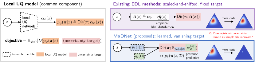
Figure 3: Overview of the EDL methods and the proposed method. Together with the white box (left), the purple box (top, right), and blue box (bottom, right) provide a high-level illustration of the existing methods in EDL and the new method MoDNet, respectively. Here, $p_{\theta}(z\mathchoice{\mspace{1.0mu}|\mspace{1.0mu}}{|}{|}{|}x)$ and $q_{\varphi}(\boldsymbol{\Pi})$ denote the cluster assignment network (Fig. 4) and the variational posterior distribution (Sec. 4.2) for VI, respectively.

4 Towards Learning Consistent Uncertainty

In EDL, each point $x$ is associated to its own meta distribution $\mathsf{Dir}(\boldsymbol{\pi};\boldsymbol{\alpha}_{\psi}(x))$. At a high level, the shortcoming of standard EDL methods stem from the absence of a proper uncertainty target for $\boldsymbol{\alpha}_{\psi}(x)$ to match. This insight leads us to construct and use a faithful uncertainty target. In this section, we introduce a new probabilistic model based on a mixture of Dirichlet distributions, and aim to learn the model based on the classical Bayesian approach, so that the consistent uncertainty is captured by design.

4.1 A Mixture of Dirichlet Distributions Model

We propose a new generative latent variable model. Recall that we denote $C$ as the number of classes. A high-level idea of our generative model assumption is that there exist $K$ clusters, where the $k$-th cluster is associated with a label distribution $\boldsymbol{\pi}^{(k)}\in\Delta^{C-1}$, for each $k\in[K]$. We assume that each image $x$ is assigned to a cluster by a cluster assignment model $p_{\theta}(z\mathchoice{\mspace{1.0mu}|\mspace{1.0mu}}{|}{|}{|}x)$ , and the associated label is then drawn from $\boldsymbol{\pi}^{(z)}$. We regard the $K$ label distributions (probability vectors) $\boldsymbol{\Pi}\mathrel{\mathop{\mathchar 58\relax missing}}=(\boldsymbol{\pi}^{(k)})_{k=1}^{K}$ as unknown parameters, and we assume a prior distribution $p(\boldsymbol{\Pi})$ based on the Bayesian principle. We aim to use the posterior distribution $p_{\theta}(\boldsymbol{\Pi}\mathchoice{\mspace{1.0mu}|\mspace{1.0mu}}{|}{|}{|}\mathcal{D})$ to define the uncertainty target for each point $x$.

We first assume the product Dirichlet distribution as a prior distribution over $\boldsymbol{\Pi}$, i.e., $p(\boldsymbol{\Pi})\mathrel{\mathop{\mathchar 58\relax missing}}=\prod_{k=1}^{K}\mathsf{Dir}(\boldsymbol{\pi}^{(k)};\mathds{1}_{C})$. Given the unknown label distributions for each cluster, we assume the following data generation process. Once a data point (say, image) $x_{n}$ is generated by the underlying data distribution $p(x)$, $x_{n}$ is assigned to one of the $K$ clusters via a discrete latent variable $z_{n}\in[K]$ via a cluster assignment model $p_{\theta}(z\mathchoice{\mspace{1.0mu}|\mspace{1.0mu}}{|}{|}{|}x)$. Then, a label $y_{n}$ is generated based on the likelihood model $p(y\mathchoice{\mspace{1.0mu}|\mspace{1.0mu}}{|}{|}{|}z,\boldsymbol{\Pi})=\boldsymbol{\pi}_{y}^{(z)}$. Mathematically, the generative model is $p_{\theta}(\{x_{n},z_{n},y_{n}\}_{n=1}^{N}\mathchoice{\mspace{1.0mu}|\mspace{1.0mu}}{|}{|}{|}\boldsymbol{\Pi})\mathrel{\mathop{\mathchar 58\relax missing}}=\prod_{n=1}^{N}p(x_{n})p_{\theta}(z_{n}\mathchoice{\mspace{1.0mu}|\mspace{1.0mu}}{|}{|}{|}x_{n})p(y_{n}\mathchoice{\mspace{1.0mu}|\mspace{1.0mu}}{|}{|}{|}z_{n},\boldsymbol{\Pi})$. Note that the only trainable component in this model is $p_{\theta}(z\mathchoice{\mspace{1.0mu}|\mspace{1.0mu}}{|}{|}{|}x)$; see Fig. 4.

Intuitively, one would expect the posterior distribution $p_{\theta}(\boldsymbol{\Pi}\mathchoice{\mspace{1.0mu}|\mspace{1.0mu}}{|}{|}{|}\mathcal{D})$ to converge, under some mild regularity assumptions, to a singular distribution whose mass is concentrated around a single point $\boldsymbol{\Pi}_{o}\in(\Delta^{C-1})^{K}$ in the infinite-sample limit, and thus the posterior predictive distribution $p_{\theta}(\boldsymbol{\pi}\mathchoice{\mspace{1.0mu}|\mspace{1.0mu}}{|}{|}{|}x,\mathcal{D})$ to be concentrated as well. This intuition underpins the introduction of this Bayesian model. We empirically demonstrate that the learned UQ model quantifies vanishing epistemic uncertainty for training data, as expected.

After fitting this model to data, we will perform inference based on the posterior predictive distribution defined as

$$p_{\theta}(\boldsymbol{\pi}\mathchoice{\mspace{1.0mu}|\mspace{1.0mu}}{|}{|}{|}x,\mathcal{D}) \mathrel{\mathop{\mathchar 58\relax missing}}=\operatorname{\mathsf{E}}_{p_{\theta}(\boldsymbol{\Pi}\mathchoice{\mspace{1.0mu}|\mspace{1.0mu}}{|}{|}{|}\mathcal{D})p_{\theta}(z\mathchoice{\mspace{1.0mu}|\mspace{1.0mu}}{|}{|}{|}x)}[p(\boldsymbol{\pi}\mathchoice{\mspace{1.0mu}|\mspace{1.0mu}}{|}{|}{|}\boldsymbol{\Pi},z)]$$

$$=\sum_{z=1}^{K}\operatorname{\mathsf{E}}_{p_{\theta}(\boldsymbol{\Pi}\mathchoice{\mspace{1.0mu}|\mspace{1.0mu}}{|}{|}{|}\mathcal{D})}[\delta(\boldsymbol{\pi}-\boldsymbol{\pi}^{(z)})].$$

Here, $p(\boldsymbol{\pi}\mathchoice{\mspace{1.0mu}|\mspace{1.0mu}}{|}{|}{|}\boldsymbol{\Pi},z)\mathrel{\mathop{\mathchar 58\relax missing}}=\delta(\boldsymbol{\pi}-\boldsymbol{\pi}^{(z)})$ denotes the Dirac delta function centered at $\boldsymbol{\pi}^{(z)}$.

Figure 4: Graphical illustration of the proposed model.

4.2 Variational Inference

To train the latent variable model, we employ the variational inference (VI) as a surrogate for the maximum likelihood estimation principle. For a variational posterior distribution $q_{\varphi}(\boldsymbol{\Pi})$ as a surrogate for the model posterior $p_{\theta}(\boldsymbol{\Pi}\mathchoice{\mspace{1.0mu}|\mspace{1.0mu}}{|}{|}{|}\mathcal{D})$, the VI objective, which is the (negative) evidence lower bound (ELBO), becomes (see Sec. B.2 for the derivation):

$$\mathsf{NELBO}(\theta,\varphi)$$ (4)

$$= D(q_{\varphi}(\boldsymbol{\Pi})~{}\|~{}p(\boldsymbol{\Pi}))+\sum_{n=1}^{N}\operatorname{\mathsf{E}}_{q_{\varphi}(\boldsymbol{\Pi})}\Bigl{[}\log\frac{1}{\operatorname{\mathsf{E}}_{p_{\theta}(z\mathchoice{\mspace{1.0mu}|\mspace{1.0mu}}{|}{|}{|}x_{n})}[\boldsymbol{\pi}_{y_{n}}^{(z)}]}\Bigr{]}.$$

To minimize the VI objective in practice, we need to choose $q_{\varphi}(\boldsymbol{\Pi})$ so that it becomes reparameterizable to allow a low-variance unbiased gradient estimator. Note that the cluster assignment probabilities $p_{\theta}(z\mathchoice{\mspace{1.0mu}|\mspace{1.0mu}}{|}{|}{|}x)$ and the variational distribution $q_{\varphi}(\boldsymbol{\Pi})$ need to be learned given $\mathcal{D}$. For the distribution over the cartesian product of probability simplexes, it is natural to consider $q_{\varphi}(\boldsymbol{\Pi})$ as a product of Dirichlet distributions $\{\mathsf{Dir}(\boldsymbol{\pi};\boldsymbol{\alpha}_{\varphi}^{(k)})\}_{k=1}^{K}$, analogous to the standard mean-field approximation. Here, $(\boldsymbol{\alpha}_{\varphi}^{(k)})_{k=1}^{K}$ are the variational parameters to be optimized.

A Dirichlet distribution, however, is not reparameterizable; thus, there is no straightforward unbiased gradient estimator concerning $\varphi$. We thus propose to use the multivariate Kumaraswamy (mvK) distribution as a reparameterizable proxy to Dirichlet distributions (Stirn et al., 2019). The mvK distribution generates a sample from the same stick-breaking process for Dirichlet distributions, but with a different base distribution called the Kumaraswamy distribution, which allows a closed-form inverse CDF. A mvK distribution is characterized by a concentration parameter as in Dirichlet distributions and has a similar form of the Dirichlet distribution with the same parameter.

4.3 Uncertainty Distillation

After training, the predictive posterior $p_{\theta}(\boldsymbol{\pi}\mathchoice{\mspace{1.0mu}|\mspace{1.0mu}}{|}{|}{|}x,\mathcal{D})$, can serve as a target distribution for the final meta distribution to be fitted to for the desired behavior for in-distribution data. However, it is not capable of quantifying sample-wise uncertainty for OOD detection, as it is designed to behave as expected only for in-distribution data, without controlling the behavior for OOD points. We also empirically observed that directly using the (approximate) predictive posterior does not directly lead to good performance in OOD detection. Since a local UQ model in EDL has proven to have such a nice capability as it fits a local meta distribution for each individual sample, we propose to exploit the best of both worlds: we train a local UQ model to distill the uncertainty from the learned posterior $p_{\theta}(\boldsymbol{\pi}\mathchoice{\mspace{1.0mu}|\mspace{1.0mu}}{|}{|}{|}x,\mathcal{D})$ in the second-stage, preserving its own local-UQ capability.

The distillation can be performed through the reverse-KL divergence minimization. That is, we train a local UQ model $p_{\psi}(\boldsymbol{\pi}\mathchoice{\mspace{1.0mu}|\mspace{1.0mu}}{|}{|}{|}x)=\mathsf{Dir}(\boldsymbol{\pi};\boldsymbol{\alpha}_{\psi}(x))$ by solving

$$\min_{\psi}\operatorname{\mathsf{E}}_{p(x)}[D(p_{\psi}(\boldsymbol{\pi}\mathchoice{\mspace{1.0mu}|\mspace{1.0mu}}{|}{|}{|}x)~{}\|~{}p_{\theta}(\boldsymbol{\pi}\mathchoice{\mspace{1.0mu}|\mspace{1.0mu}}{|}{|}{|}x,\mathcal{D}))].$$

We approximate the intractable term $p_{\theta}(\boldsymbol{\pi}\mathchoice{\mspace{1.0mu}|\mspace{1.0mu}}{|}{|}{|}x,\mathcal{D})$ as

$$p_{\theta}(\boldsymbol{\pi}\mathchoice{\mspace{1.0mu}|\mspace{1.0mu}}{|}{|}{|}x,\mathcal{D}) \stackrel{{\scriptstyle\mathchoice{\hbox to0.0pt{\hss$\displaystyle{(a)}$\hss}}{\hbox to0.0pt{\hss$\textstyle{(a)}$\hss}}{\hbox to0.0pt{\hss$\scriptstyle{(a)}$\hss}}{\hbox to0.0pt{\hss$\scriptscriptstyle{(a)}$\hss}}}}{{\approx}}\operatorname{\mathsf{E}}_{q_{\varphi}(\boldsymbol{\Pi})p_{\theta}(z\mathchoice{\mspace{1.0mu}|\mspace{1.0mu}}{|}{|}{|}x)}[p(\boldsymbol{\pi}\mathchoice{\mspace{1.0mu}|\mspace{1.0mu}}{|}{|}{|}\boldsymbol{\Pi},z)]$$

$$\stackrel{{\scriptstyle\mathchoice{\hbox to0.0pt{\hss$\displaystyle{(b)}$\hss}}{\hbox to0.0pt{\hss$\textstyle{(b)}$\hss}}{\hbox to0.0pt{\hss$\scriptstyle{(b)}$\hss}}{\hbox to0.0pt{\hss$\scriptscriptstyle{(b)}$\hss}}}}{{\approx}}\operatorname{\mathsf{E}}_{p_{\theta}(z\mathchoice{\mspace{1.0mu}|\mspace{1.0mu}}{|}{|}{|}x)}[\mathsf{Dir}(\boldsymbol{\pi};\boldsymbol{\alpha}_{\varphi}^{(z)})]$$

$$\stackrel{{\scriptstyle\mathchoice{\hbox to0.0pt{\hss$\displaystyle{(c)}$\hss}}{\hbox to0.0pt{\hss$\textstyle{(c)}$\hss}}{\hbox to0.0pt{\hss$\scriptstyle{(c)}$\hss}}{\hbox to0.0pt{\hss$\scriptscriptstyle{(c)}$\hss}}}}{{\approx}}\mathsf{Dir}(\boldsymbol{\pi};\operatorname{\mathsf{E}}_{p_{\theta}(z\mathchoice{\mspace{1.0mu}|\mspace{1.0mu}}{|}{|}{|}x)}[\boldsymbol{\alpha}_{\varphi}^{(z)}]).$$ (5)

Here, $(a)$ follows from replacing the posterior $p_{\theta}(\boldsymbol{\Pi}\mathchoice{\mspace{1.0mu}|\mspace{1.0mu}}{|}{|}{|}\mathcal{D})$ with the variational posterior $q_{\varphi}(\boldsymbol{\Pi})$; $(b)$ follows by regarding the learned concentration parameters under mvK distributions as the those under Dirichlet distributions for the sake of computational efficiency; $(c)$ becomes tight if and only if the cluster assignment distribution $(p_{\theta}(z\mathchoice{\mspace{1.0mu}|\mspace{1.0mu}}{|}{|}{|}x))_{z\in[K]}$ is a one-hot vector for every $x$. Letting $\boldsymbol{\alpha}_{\theta,\varphi}^{\mathsf{target}}(x)\mathrel{\mathop{\mathchar 58\relax missing}}=\operatorname{\mathsf{E}}_{p_{\theta}(z\mathchoice{\mspace{1.0mu}|\mspace{1.0mu}}{|}{|}{|}x)}[\boldsymbol{\alpha}_{\varphi}^{(z)}]$, we regard $\mathsf{Dir}(\boldsymbol{\pi};\boldsymbol{\alpha}_{\theta,\varphi}^{\mathsf{target}}(x))$ as a whole as the target for the final meta distribution, and the reverse-KL objective can then be approximated and upper bounded as

$$\operatorname{\mathsf{E}}_{p(x)}[D(p_{\psi}(\boldsymbol{\pi}\mathchoice{\mspace{1.0mu}|\mspace{1.0mu}}{|}{|}{|}x)~{}\|~{}p_{\theta}(\boldsymbol{\pi}\mathchoice{\mspace{1.0mu}|\mspace{1.0mu}}{|}{|}{|}x,\mathcal{D}))]$$

$$\stackrel{{\scriptstyle\mathchoice{\hbox to0.0pt{\hss$\displaystyle{\eqref{eq:approx_posterior}}$\hss}}{\hbox to0.0pt{\hss$\textstyle{\eqref{eq:approx_posterior}}$\hss}}{\hbox to0.0pt{\hss$\scriptstyle{\eqref{eq:approx_posterior}}$\hss}}{\hbox to0.0pt{\hss$\scriptscriptstyle{\eqref{eq:approx_posterior}}$\hss}}}}{{\approx}}\operatorname{\mathsf{E}}_{p(x)}\bigl{[}D(p_{\psi}(\boldsymbol{\pi}\mathchoice{\mspace{1.0mu}|\mspace{1.0mu}}{|}{|}{|}x)~{}\|~{}\mathsf{Dir}(\boldsymbol{\pi};\boldsymbol{\alpha}_{\theta,\varphi}^{\mathsf{target}}(x)))\bigr{]},$$ (6)

The final objective is (6) to fit the local UQ model $p_{\psi}(\boldsymbol{\pi}\mathchoice{\mspace{1.0mu}|\mspace{1.0mu}}{|}{|}{|}x)$.

We call the entire model and training method the Mixture of Dirichlet distributions Network, MoDNet in short. In what follows, we indicate the mode of parameterization as a subscript, i.e., MoDNet_direct and MoDNet_density. See Fig. 3 for a comparison to the standard EDL methods.

5 Experiments

We demonstrate the superior empirical performance of our proposed method from two perspectives. First, we conduct a comprehensive comparison between our proposed approach and existing EDL-based methods on UQ downstream tasks. Next, we delve deeper into revealing the inconsistency issue of existing approaches, and substantiate how MoDNet can effectively mitigate the issue. More results and implementation details can be found in Sec. D and C.

5.1 Experiment Settings

Baselines. We focus on comparing representative EDL methods, including (1) RPriorNet (Malinin & Gales, 2019), (2) PostNet (Charpentier et al., 2020), (3) Belief Matching (BM) (Joo et al., 2020). We omit the comparison with ensemble distribution distillation method (Malinin et al., 2020) due to its training instability and sensitivity to hyper-parameter tuning. In addition, we also include two classical UQ methods: (1) Deep Ensemble (Ensemble) (Lakshminarayanan et al., 2017) that trains multiple models with different random initialization; (2) Monte Carlo Dropout (Dropout) (Gal & Ghahramani, 2016) that approximates the Bayesian inference using random dropout.

Benchmark. We conduct an extensive evaluation using three in-distribution datasets to train the uncertainty models: MNIST, CIFAR10, and CIFAR100. For the OOD detection task, we select four OOD datasets for each in-distribution dataset: we use Omiglot, FashionMNIST, KMNIST, and corrupted MNIST as OOD datasets for MNIST; we use SVHN, FMNIST, TinyImageNet, and corrupted CIFAR10 (CIFAR100) as OOD datasets for CIFAR10 (CIFAR100).

Implementation Details. For different datasets, we employ different base architectures: a simple convolution neural network for MNIST, VGG16 (Simonyan & Zisserman, 2014) for CIFAR10, and ResNet18 (He et al., 2016) for CIFAR100. For quantifying different types of uncertainties, we use uncertainty metrics defined in Section 2.3. We evaluate the UQ downstream performance through the Area Under the ROC Curve (AUROC) and Area Under the Precision-Recall Curve (AUPR). When computing these, we treat in-distribution (correctly classified) test samples as the negative class and outlier (misclassified) samples as the positive class. Reported numbers are averaged over five runs.

5.2 UQ Downstream Tasks

We consider two UQ downstream tasks: (1) OOD data detection, where the goal is to identify the OOD data based on the learned epistemic uncertainty; (2) Selective classification, where the goal is to identify the wrongly predicted samples at the test stage based on total uncertainty, as wrong prediction can occur from either high epistemic or high aleatoric uncertainty, or both. A model with desired UQ capability is expected to output high uncertainties for OOD (wrong predicted) samples, while outputting low uncertainty for in-distribution (correctly predicted) samples.

Results. The OOD detection AUROC results are presented in Table 2; see Table 6 for AUPR results and Table 8 for CIFAR100 in Appendix. The results reveal the advantage of EDL methods over the classical UQ approaches, primarily attributed to their strong capability to capture epistemic uncertainty. On the three benchmark datasets, our proposed approaches consistently yield comparable or better AUROC scores than existing SOTA EDL methods. The Selective Classification AUROC results are presented in Table 3 (see Table 7 for AUPR results and Table 9 for CIFAR100 in Appendix). Across all three benchmark datasets, MoDNet consistently outperforms the existing EDL-based approaches. It is important to note that while Bayesian UQ methods (Ensemble and Dropout) demonstrate strong performance, they necessitate significantly more computational resources.

Table 2: OOD Detection AUROC score. MI and DEnt stand for Mutual Information and Differential Entropy. The first row in the header indicates the ID data and the second the OOD data. FMNIST and TImageNet are shorthands for FashionMNIST and TinyImageNet.

Methods	Metric	MNIST				CIFAR10
		Omniglot	FMNIST	KMNIST	Corrupted	SVHN	FMNIST	TImageNet	Corrupted
Ensemble	MI	$99.5_{\pm 0.0}$	$87.0_{\pm 0.3}$	$89.5_{\pm 0.2}$	$99.0_{\pm 0.1}$	$74.2_{\pm 0.7}$	$75.0_{\pm 0.6}$	$73.7_{\pm 0.4}$	$77.9_{\pm 0.3}$
Dropout	MI	$82.9_{\pm 0.1}$	$78.1_{\pm 0.1}$	$69.4_{\pm 0.1}$	$97.8_{\pm 0.0}$	$58.3_{\pm 0.0}$	$56.8_{\pm 0.0}$	$54.3_{\pm 0.0}$	$71.5_{\pm 0.0}$
R-KL PriorNet	MI	$\bf 99.9_{\pm 0.1}$	$97.7_{\pm 0.9}$	$94.8_{\pm 0.7}$	$\bf 99.9_{\pm 0.0}$	$37.3_{\pm 21.2}$	$51.5_{\pm 13.4}$	$48.1_{\pm 10.9}$	$51.7_{\pm 29.4}$
	DEnt	$\bf 99.9_{\pm 0.1}$	$97.7_{\pm 0.8}$	$94.6_{\pm 0.8}$	$\bf 99.9_{\pm 0.0}$	$66.8_{\pm 24.3}$	$73.7_{\pm 7.7}$	$65.5_{\pm 8.3}$	$77.4_{\pm 25.7}$
BM	MI	$\bf 99.9_{\pm 0.1}$	$98.0_{\pm 2.4}$	$96.7_{\pm 0.8}$	$\bf 99.9_{\pm 0.1}$	$94.9_{\pm 3.2}$	$\bf 90.0_{\pm 1.8}$	$81.2_{\pm 5.1}$	$97.1_{\pm 0.1}$
	DEnt	$\bf 99.9_{\pm 0.1}$	$98.0_{\pm 2.3}$	$96.6_{\pm 0.9}$	$\bf 99.9_{\pm 0.1}$	$95.5_{\pm 3.4}$	$\bf 91.0_{\pm 1.7}$	$84.5_{\pm 3.2}$	$\bf 97.5_{\pm 0.1}$
PostNet	MI	$99.1_{\pm 0.7}$	$98.8_{\pm 0.3}$	$96.2_{\pm 1.4}$	$99.4_{\pm 0.4}$	$89.0_{\pm 4.6}$	$86.7_{\pm 2.2}$	$84.5_{\pm 1.2}$	$92.6_{\pm 6.6}$
	DEnt	$99.4_{\pm 0.1}$	$99.1_{\pm 0.2}$	$97.1_{\pm 1.0}$	$99.5_{\pm 0.4}$	$89.4_{\pm 4.5}$	$87.2_{\pm 2.1}$	$84.9_{\pm 1.2}$	$93.0_{\pm 6.3}$
MoDNetdensity	MI	$99.5_{\pm 0.3}$	$99.0_{\pm 0.8}$	$96.9_{\pm 0.3}$	$\bf 99.9_{\pm 0.1}$	$93.1_{\pm 0.7}$	$86.6_{\pm 2.9}$	$84.4_{\pm 2.0}$	$95.9_{\pm 1.2}$
	DEnt	$99.6_{\pm 0.2}$	$99.2_{\pm 0.7}$	$97.2_{\pm 0.3}$	$\bf 99.9_{\pm 0.1}$	$93.1_{\pm 0.6}$	$86.4_{\pm 2.9}$	$84.5_{\pm 2.0}$	$95.8_{\pm 1.1}$
MoDNetdirect	MI	$\bf 99.9_{\pm 0.1}$	$\bf 99.7_{\pm 0.1}$	$\bf 98.7_{\pm 0.3}$	$\bf 99.9_{\pm 0.1}$	$\bf 95.0_{\pm 1.5}$	$89.2_{\pm 1.6}$	$\bf 86.2_{\pm 0.9}$	$95.7_{\pm 2.7}$
	DEnt	$\bf 99.9_{\pm 0.2}$	$\bf 99.7_{\pm 0.1}$	$\bf 98.6_{\pm 0.3}$	$\bf 99.9_{\pm 0.2}$	$\bf 96.\par 0_{\pm 1.3}$	$\bf 91.3_{\pm 1.3}$	$\bf 86.7_{\pm 1.4}$	$96.9_{\pm 1.5}$

Table 3: Performance evaluation for selective classification. Ent and MaxP stand for Entropy and Max Probability, respectively.

Methods	Metric	MNIST		CIFAR10
		Test Acc	AUROC	Test Acc	AUROC
Ensemble	Ent	$99.7_{\pm 0.0}$	$\bf 99.2_{\pm 0.0}$	$92.6_{\pm 0.0}$	$91.3_{\pm 0.1}$
	MaxP	$99.7_{\pm 0.0}$	$\bf 99.2_{\pm 0.0}$	$92.6_{\pm 0.0}$	$\bf 92.4_{\pm 0.2}$
Dropout	Ent	$99.4_{\pm 0.0}$	$98.3_{\pm 0.1}$	$85.9_{\pm 0.0}$	$88.9_{\pm 0.1}$
	MaxP	$99.4_{\pm 0.0}$	$98.3_{\pm 0.2}$	$85.9_{\pm 0.0}$	$89.1_{\pm 0.1}$
RPriorNet	Ent	$99.4_{\pm 0.0}$	$91.7_{\pm 1.2}$	$84.7_{\pm 2.8}$	$74.1_{\pm 4.7}$
	MaxP	$99.4_{\pm 0.0}$	$91.8_{\pm 1.2}$	$84.7_{\pm 2.8}$	$79.5_{\pm 4.2}$
BM	Ent	$99.5_{\pm 0.0}$	$95.0_{\pm 0.6}$	$88.5_{\pm 0.5}$	$89.2_{\pm 0.6}$
	MaxP	$99.5_{\pm 0.0}$	$95.0_{\pm 0.6}$	$88.5_{\pm 0.5}$	$89.2_{\pm 0.6}$
PostNet	Ent	$99.4_{\pm 0.1}$	$95.8_{\pm 2.0}$	$88.5_{\pm 0.3}$	$89.1_{\pm 0.4}$
	MaxP	$99.4_{\pm 0.1}$	$95.8_{\pm 2.0}$	$88.5_{\pm 0.3}$	$89.1_{\pm 0.3}$
MoDNetdensity	Ent	$98.3_{\pm 0.2}$	$\mathbf{98.5}_{\pm 0.5}$	$87.9_{\pm 0.6}$	$88.1_{\pm 1.5}$
	MaxP	$98.3_{\pm 0.2}$	$\mathbf{98.5}_{\pm 0.5}$	$87.9_{\pm 0.6}$	$88.1_{\pm 1.5}$
MoDNetdirect	Ent	$99.3_{\pm 0.0}$	$97.0_{\pm 1.1}$	$88.6_{\pm 0.9}$	$\mathbf{90.2}_{\pm 0.3}$
	MaxP	$99.3_{\pm 0.0}$	$97.0_{\pm 1.1}$	$88.6_{\pm 0.9}$	$\mathbf{90.2}_{\pm 0.3}$

Discussion. For a fair comparison, we used the same base model architecture for all methods. The primary distinction between MoDNet and other EDL methods lies in adopting different uncertainty targets. The UQ downstream performance further demonstrates the effectiveness of our approach over the fixed uncertainty target. Interestingly, the results indicate that the density parameterization does not enhance the UQ performance over the direct parameterization, both in MoDNet and EDL baselines, indicating that direct parameterization can be considered the first choice in practice. The counter-intuitive results might be due to the limited expressiveness of the flow model.

5.3 Consistent Epistemic Uncertainty Quantification

In the previous section, most of the EDL baselines showed promising performance on the UQ downstream tasks, aligned with the findings in the literature. The issue demonstrated in Sec. 3 and Fig. 1 does not kick in these tasks, as there is no comparison over different models trained with different sample sizes, and the best $\lambda$ was used for each method for given datasets. However, we remark that, if a practitioner deploys the learned epistemic uncertainty to design a system, expecting the epistemic uncertainty to vanish as she acquires more data, the standard EDL methods could potentially lead to an unexpected consequence.

In this section, we aim to empirically demonstrate the vulnerabilities and potential risk of the inconsistently learned epistemic uncertainty in existing EDL methods in the model selection problem in multi-source domain adaptation. This will demonstrate how the consistently learned epistemic uncertainty quantification plays a crucial role.

5.3.1 Empirical Demonstration

Before we proceed, we remark on the demonstration of the (in)consistency in the learned epistemic uncertainty in Fig. 1, where Fig. 5(a) presents the complete set of experimental results with varying $\lambda$ and different parameterization (direct or density). Here, we investigate the behavior of the learned epistemic uncertainty of EDL methods and MoDNet by tracking the averaged MI $\operatorname{\mathsf{E}}_{p(x)}[I_{\psi}(y;\boldsymbol{\pi}\mathchoice{\mspace{1.0mu}|\mspace{1.0mu}}{|}{|}{|}x)]$ on a test set in relation to the size of training data, with a simple dataset of a mixture of three Gaussians in $\mathbb{R}^{2}$. We sampled data of varying sizes ($N\in\{100,200,500,1000,2000,5000\}$) to create different training datasets to train the UQ models and maintain a single test dataset with fixed size ($N=2000$) to evaluate their test accuracy and averaged epistemic uncertainty. We trained a simple neural-network EDL model using the reverse KL objective with $\lambda=\nu^{-1}\in\{10^{-1},10^{-2},10^{-3}\}$, with direct and density parameterization, corresponding to belief matching (BM) and PostNet, respectively. As predicted by Lemma 3.1, the MI is almost constant with respect to the sample size for the existing EDL methods, as observed in the first three columns of Fig. 5(a). Additionally, the scale of epistemic uncertainty also varies as a different $\lambda$ is used. On the other hand, our model MoDNet present monotonically decreasing and eventually vanishing epistemic uncertainty for in-distribution test data.

We further demonstrate the issue with MNIST dataset. As before, we varied the training data size ($N\in\{1000,2000,5000,10000,20000,50000\}$) to train the UQ models and evaluated the test accuracy and averaged epistemic uncertainty of each model using a test dataset of fixed size ($N=10000$). The results are shown in Fig. 5(b). A similar behavior is exhibited as in the toy example, which further corroborates that the learned uncertainty from the standard EDL approach is not being learned in a faithful way, whereas our MoDNet can effectively mitigate this issue.

Table 4: Performance evaluation for model selection. The numbers in the table indicate the gap in accuracy (%) between the best and retrieved models. Lower accuracy gap indicates better model selection, and zero value indicates perfect model selection. SDigits stands for Synthetic Digits dataset.

Methods	MNIST	SVHN	USPS	MNIST-M	SDigits	Avg.
PostNet (fixed $\lambda$)	$12.6_{\pm 6.5}$	$\bf 0.0_{\pm 0.0}$	$\bf 0.0_{\pm 0.0}$	$\bf 0.0_{\pm 0.0}$	$2.8_{\pm 2.3}$	3.1
BM (fixed $\lambda$)	$17.7_{\pm 1.2}$	$8.6_{\pm 7.2}$	$\bf 0.0_{\pm 0.0}$	$\bf 0.0_{\pm 0.0}$	$15.1_{\pm 7.7}$	8.3
PostNet (tuned $\lambda$)	$6.6_{\pm 9.0}$	$8.1_{\pm 4.1}$	$53.6_{\pm 1.1}$	$23.9_{\pm 29.5}$	$2.1_{\pm 2.0}$	18.9
BM (tuned $\lambda$)	$6.2_{\pm 4.0}$	$7.9_{\pm 6.8}$	$43.6_{\pm 3.8}$	$33.5_{\pm 27.5}$	$2.3_{\pm 4.6}$	18.7
MoDNetdensity	$\bf 0.0_{\pm 0.0}$	$4.2_{\pm 4.2}$	$\bf 0.0_{\pm 0.0}$	$\bf 0.0_{\pm 0.0}$	$1.6_{\pm 1.8}$	$\bf 1.2$
MoDNetdirect	$\bf 0.0_{\pm 0.0}$	$6.1_{\pm 5.2}$	${\bf 0.0_{\pm 0.0}}$	${\bf 0.0_{\pm 0.0}}$	${\bf 1.3_{\pm 1.5}}$	1.5

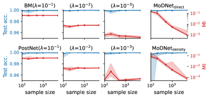
(a)

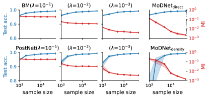
(b)

Figure 5: Epistemic Uncertainty and Test Accuracy v.s. Number of Training Data. Existing methods (BM and PostNet) fail to learn consistent epistemic uncertainty. Learned uncertainty from our UQ model (with either direct or density parameterization) monotonically vanishes as the sample size increases, as shown in the last column.

5.3.2 Application: Model Selection in Multi-Source Domain Adaptation

As we introduced in Section 5.2, selective classification abstains from predictions with high total uncertainty to mitigate the risk of making mistakes. A similar type of abstention, but at a higher level, can be useful in other applications, such as multi-source domain adaptation; see Appendix D.2. Suppose that we wish to make predictions on a target task, given multiple pre-trained models, where not all of them are capable of making accurate predictions. Without additional label information from the target task, it is reasonable to use model’s epistemic uncertainty on the target task to select the best model. Intuitively, high epistemic uncertainty indicates the model’s insufficient knowledge about the target task, and we should avoid selecting such a model.

Formally, given multiple pre-trained UQ models $\{\theta_{j}\}_{j=1}^{m}$ trained on $m$ source domains, and a target domain dataset $\mathcal{D}^{t}=\{(x^{t}_{n},y^{t}_{n})\}_{n=1}^{N}$, we aim to identify the optimal pre-trained UQ model that can achieve best prediction accuracy on $\mathcal{D}^{t}$ based on the average epistemic uncertainty evaluated on $\mathcal{D}^{t}$. Specifically, the epistemic uncertainty of of $j$-th source model evaluated on $\mathcal{D}^{t}$ is obtained using the average mutual information, i.e., $\mathsf{MI}_{j}\mathrel{\mathop{\mathchar 58\relax missing}}=\frac{1}{N}\sum_{n=1}^{N}I_{\theta_{j}}(y;\boldsymbol{\pi}\mathchoice{\mspace{1.0mu}|\mspace{1.0mu}}{|}{|}{|}x^{t}_{n})$. Then, the optimal model is obtained by selecting the model with the lowest epistemic uncertainty, i.e., $\theta^{*}=\theta_{\arg\min_{j\in[m]}\mathsf{MI}_{j}}$. This task requires epistemic uncertainty to be well-calibrated at the model level, i.e., as source models are pre-trained using datasets with different sizes and data distributions, the epistemic uncertainty should reflect these factors and maintain comparability across models. As we discussed in Sec. 5.3.1, existing EDL approaches usually cannot meet such requirements.

We provide an empirical evaluation using the DigitsFive benchmark, which contains five different domains of digit recognition tasks, including MNIST, SVHN, USPS, MNISTM, and Synthetic Digits. Assuming the pre-trained UQ models on these five domain datasets are available, we randomly pick pre-trained models of four domains, and treat the remaining domain as target task to be tested on, resulting in the total five model selection tasks. We evaluate the test accuracy of the selected model among the other four candidates and compare it with the the actual best model by reporting the gap in accuracy (%).

To compare MoDNet with PostNet and BM, we consider two different settings to train the baselines: (1) use a fixed regularization weight $\lambda=10^{-3}$ to train the models with different domains; (2) select the best $\lambda$ based on validation accuracy evaluated on the source task, where $\lambda$ might be different for different domains. Note that (2) better reflects a practical setup, as tuning the hyperparameter using a validation set is common. The results are summarized in Table 4. It can be seen that with the best $\lambda$’s, the baselines fail to identify the optimal model for all the five tasks due to un-calibrated scales in the measured uncertainty. In contrast, MoDNet can achieve much smaller accuracy gaps than the baseline methods by quantifying more calibrated epistemic uncertainties, coherent with its very definition.

6 Concluding Remarks

Our work calls for the community’s attention to the inconsistency in the learned epistemic uncertainty based on the existing methods in evidential deep learning. We propose a new evidential deep learning method that outputs predictive epistemic uncertainty, demonstrating consistent behavior in accordance with its own definition. We exhibit the superior performance of the new method MoDNet in the standard UQ downstream tasks, as well as demonstrate its potential ability in a model selection problem. An exciting future direction is to explore the idea beyond classification, as in, e.g., a recent attempt of Charpentier et al. (2022).

Appendix A Details of Existing EDL Objectives

A.1 Prior Network Objective

Prior networks (Malinin & Gales, 2018, 2019) proposed to use the following form of objectives:

$$\operatorname{\mathsf{E}}_{p(x,y)}[D({p_{\nu}(\boldsymbol{\pi}\mathchoice{\mspace{1.0mu}|\mspace{1.0mu}}{|}{|}{|}y)},{p_{\psi}(\boldsymbol{\pi}\mathchoice{\mspace{1.0mu}|\mspace{1.0mu}}{|}{|}{|}x)})+\gamma_{\mathsf{ood}}\operatorname{\mathsf{E}}_{p_{\textsf{ood}}(x)}[D({p(\boldsymbol{\pi})},{p_{\psi}(\boldsymbol{\pi}\mathchoice{\mspace{1.0mu}|\mspace{1.0mu}}{|}{|}{|}x)})].$$

Here, $\nu(\in\{10^{2},10^{3}\})$ and $\gamma_{\mathsf{ood}}$ are hyperparameters.

• The F-KL objective (Malinin & Gales, 2018) is when $D(p,q)=D(p~{}\|~{}q)$. The in-distribution objective can be written as

  $$\operatorname{\mathsf{E}}_{p(x,y)}[D({p_{\nu}(\boldsymbol{\pi}\mathchoice{\mspace{1.0mu}|\mspace{1.0mu}}{|}{|}{|}y)}~{}\|~{}{p_{\psi}(\boldsymbol{\pi}\mathchoice{\mspace{1.0mu}|\mspace{1.0mu}}{|}{|}{|}x)})]=\operatorname{\mathsf{E}}_{p(x)}[D(\operatorname{\mathsf{E}}_{p(y\mathchoice{\mspace{1.0mu}|\mspace{1.0mu}}{|}{|}{|}x)}[p_{\nu}(\boldsymbol{\pi}\mathchoice{\mspace{1.0mu}|\mspace{1.0mu}}{|}{|}{|}y)]~{}\|~{}p_{\psi}(\boldsymbol{\pi}\mathchoice{\mspace{1.0mu}|\mspace{1.0mu}}{|}{|}{|}x))]+\mathsf{(const.)}.$$

  This implies that minimizing the F-KL objective function forces the unimodal UQ model $p_{\psi}(\boldsymbol{\pi}\mathchoice{\mspace{1.0mu}|\mspace{1.0mu}}{|}{|}{|}x)$ to fit the mixture of Dirichlet distributions $\operatorname{\mathsf{E}}_{p(y\mathchoice{\mspace{1.0mu}|\mspace{1.0mu}}{|}{|}{|}x)}[p_{\nu}(\boldsymbol{\pi}\mathchoice{\mspace{1.0mu}|\mspace{1.0mu}}{|}{|}{|}y)]$. Since the mixture can be multimodal when $p(y\mathchoice{\mspace{1.0mu}|\mspace{1.0mu}}{|}{|}{|}x)$ is not one-hot, or equivalently, if aleatoric uncertainty is nonzero, the F-KL objective will drive the UQ model to spread the probability mass over the simplex, which possibly leads to low accuracy.

• The R-KL objective (Malinin & Gales, 2019) is when $D(p,q)=D(q~{}\|~{}p)$. Unlike the F-KL objective, the in-distribution objective can be written as

  $$\operatorname{\mathsf{E}}_{p(x,y)}[D({p_{\psi}(\boldsymbol{\pi}\mathchoice{\mspace{1.0mu}|\mspace{1.0mu}}{|}{|}{|}x)}~{}\|~{}{p_{\nu}(\boldsymbol{\pi}\mathchoice{\mspace{1.0mu}|\mspace{1.0mu}}{|}{|}{|}y)})]=\operatorname{\mathsf{E}}_{p(x)}[D({p_{\psi}(\boldsymbol{\pi}\mathchoice{\mspace{1.0mu}|\mspace{1.0mu}}{|}{|}{|}x)}~{}\|~{}\mathsf{Dir}(\boldsymbol{\pi};\boldsymbol{\alpha}_{0}+\nu\boldsymbol{\eta}(x)))]+\mathsf{(const.)}.$$

  Since $p_{\psi}(\boldsymbol{\pi}\mathchoice{\mspace{1.0mu}|\mspace{1.0mu}}{|}{|}{|}x)$ is being fit to another Dirichlet distribution $\mathsf{Dir}(\boldsymbol{\pi};\boldsymbol{\alpha}_{0}+\nu\boldsymbol{\eta}(x))$, it no longer has the issue of the F-KL objective above. We note in passing that Nandy et al. (2020) proposed an ad-hoc objective such that $\boldsymbol{\alpha}_{\psi}(x)<1$ for OOD $x$’s.

A.2 Variational Inference Objective

The variational inference (VI) loss was proposed by Chen et al. (2018); Joo et al. (2020) in the following form:

$$\ell_{\textsf{VI}}(\psi;x,y)\mathrel{\mathop{\mathchar 58\relax missing}}=\operatorname{\mathsf{E}}_{p_{\psi}(\boldsymbol{\pi}\mathchoice{\mspace{1.0mu}|\mspace{1.0mu}}{|}{|}{|}x)}\Bigl{[}\log\frac{1}{p(y\mathchoice{\mspace{1.0mu}|\mspace{1.0mu}}{|}{|}{|}\boldsymbol{\pi})}\Bigr{]}+\lambda D(p_{\psi}(\boldsymbol{\pi}\mathchoice{\mspace{1.0mu}|\mspace{1.0mu}}{|}{|}{|}x)~{}\|~{}p(\boldsymbol{\pi})).$$ (7)

Although the original derivation is a bit involved, we can rephrase the key logic in the paper by the following variational relaxation:

$$D(p(x,y)~{}\|~{}p(x)p_{\lambda^{-1}}(y))\leq D(p(x,y)p_{\psi}(\boldsymbol{\pi}\mathchoice{\mspace{1.0mu}|\mspace{1.0mu}}{|}{|}{|}x)~{}\|~{}p(x)p_{\lambda^{-1}}(\boldsymbol{\pi},y)),$$

where $p_{\nu}(y)$ is induced by the tempered distribution $p_{\nu}(\boldsymbol{\pi},y)\propto p(\boldsymbol{\pi})p^{\nu}(y\mathchoice{\mspace{1.0mu}|\mspace{1.0mu}}{|}{|}{|}\boldsymbol{\pi})$. The inequality is a simple application of a form of data processing inequality (Cover & Thomas, 2006). We remark that the original name, “ELBO loss,” is a misnomer for this loss function, as the right-hand side simply bounds a constant on the left-hand side, as opposed to the negative ELBO, which bounds the negative log-likelihood.

Lemma A.1.

Let $\nu\mathrel{\mathop{\mathchar 58\relax missing}}=\lambda^{-1}$. Then, we have

$$\min_{\psi}\operatorname{\mathsf{E}}_{p(x,y)}[\ell_{\mathsf{VI}}(\psi;x,y)]\equiv\min_{\psi}\operatorname{\mathsf{E}}_{p(x,y)}[D(p_{\psi}(\boldsymbol{\pi}\mathchoice{\mspace{1.0mu}|\mspace{1.0mu}}{|}{|}{|}x)~{}\|~{}p_{\nu}(\boldsymbol{\pi}\mathchoice{\mspace{1.0mu}|\mspace{1.0mu}}{|}{|}{|}y))].$$

Proof.

Note that by the chain rule of KL divergence, we have on the one hand

$$D(p(x,y)p_{\psi}(\boldsymbol{\pi}\mathchoice{\mspace{1.0mu}|\mspace{1.0mu}}{|}{|}{|}x)~{}\|~{}p(x)p_{\nu}(\boldsymbol{\pi},y))=D(p(x,y)~{}\|~{}p(x)p_{\nu}(y))+\operatorname{\mathsf{E}}_{p(x,y)}[D(p_{\psi}(\boldsymbol{\pi}\mathchoice{\mspace{1.0mu}|\mspace{1.0mu}}{|}{|}{|}x)~{}\|~{}p_{\nu}(\boldsymbol{\pi}\mathchoice{\mspace{1.0mu}|\mspace{1.0mu}}{|}{|}{|}y)].$$

Hence,

$$\min_{\psi}\operatorname{\mathsf{E}}_{p(x,y)}[D(p_{\psi}(\boldsymbol{\pi}\mathchoice{\mspace{1.0mu}|\mspace{1.0mu}}{|}{|}{|}x)~{}\|~{}p_{\nu}(\boldsymbol{\pi}\mathchoice{\mspace{1.0mu}|\mspace{1.0mu}}{|}{|}{|}y))]\equiv\min_{\psi}D(p(x,y)p_{\psi}(\boldsymbol{\pi}\mathchoice{\mspace{1.0mu}|\mspace{1.0mu}}{|}{|}{|}x)~{}\|~{}p(x)p_{\nu}(\boldsymbol{\pi},y)).$$ (8)

On the other hand, we have

$$D(p(x,y)p_{\psi}(\boldsymbol{\pi}\mathchoice{\mspace{1.0mu}|\mspace{1.0mu}}{|}{|}{|}x)~{}\|~{}p(x)p_{\nu}(\boldsymbol{\pi},y))$$

$$=\operatorname{\mathsf{E}}_{p(x,y)p_{\psi}(\boldsymbol{\pi}\mathchoice{\mspace{1.0mu}|\mspace{1.0mu}}{|}{|}{|}x)}\Bigl{[}\log\frac{p(x,y)p_{\psi}(\boldsymbol{\pi}\mathchoice{\mspace{1.0mu}|\mspace{1.0mu}}{|}{|}{|}x)}{p(x)p_{\nu}(\boldsymbol{\pi},y)}\Bigr{]}$$

$$=\operatorname{\mathsf{E}}_{p(x,y)q_{\psi}(\boldsymbol{\pi}\mathchoice{\mspace{1.0mu}|\mspace{1.0mu}}{|}{|}{|}x)}\Bigl{[}\log\frac{p(x,y)p_{\psi}(\boldsymbol{\pi}\mathchoice{\mspace{1.0mu}|\mspace{1.0mu}}{|}{|}{|}x)}{p(x)p(\boldsymbol{\pi})p^{\nu}(y\mathchoice{\mspace{1.0mu}|\mspace{1.0mu}}{|}{|}{|}\boldsymbol{\pi})}\Bigr{]}+\log B$$

$$=\operatorname{\mathsf{E}}_{p(x,y)}\Bigl{[}\nu\operatorname{\mathsf{E}}_{p_{\psi}(\boldsymbol{\pi}\mathchoice{\mspace{1.0mu}|\mspace{1.0mu}}{|}{|}{|}x)}\Bigl{[}\log\frac{1}{p(y\mathchoice{\mspace{1.0mu}|\mspace{1.0mu}}{|}{|}{|}\boldsymbol{\pi})}\Bigr{]}+D(p_{\psi}(\boldsymbol{\pi}\mathchoice{\mspace{1.0mu}|\mspace{1.0mu}}{|}{|}{|}x)~{}\|~{}p(\boldsymbol{\pi}))\Bigr{]}+D(p(x,y)~{}\|~{}p(x))+\log B$$

$$=\operatorname{\mathsf{E}}_{p(x,y)}[\ell_{\mathsf{VI}}(\psi;x,y)]+D(p(x,y)~{}\|~{}p(x))+\log B.$$

Here, we let $B\mathrel{\mathop{\mathchar 58\relax missing}}=\sum_{y}\int p(\boldsymbol{\pi})p^{\nu}(y\mathchoice{\mspace{1.0mu}|\mspace{1.0mu}}{|}{|}{|}\boldsymbol{\pi})\mathop{}\!\mathrm{d}\boldsymbol{\pi}$ is the normalization constant, which satisfies $p_{\nu}(\boldsymbol{\pi},y)=\frac{1}{B}p(\boldsymbol{\pi})p^{\nu}(y\mathchoice{\mspace{1.0mu}|\mspace{1.0mu}}{|}{|}{|}\boldsymbol{\pi})$. This implies that

$$\min_{\psi}D(p(x,y)p_{\psi}(\boldsymbol{\pi}\mathchoice{\mspace{1.0mu}|\mspace{1.0mu}}{|}{|}{|}x)~{}\|~{}p(x)p_{\nu}(\boldsymbol{\pi},y))\equiv\min_{\psi}\operatorname{\mathsf{E}}_{p(x,y)}[\ell_{\mathsf{VI}}(\psi;x,y)].$$ (9)

Combining (9) and (8), we prove the desired equivalence. ∎

A.3 Uncertainty Cross Entropy Objective

Charpentier et al. (2020, 2022) proposed to use the uncertainty cross-entropy loss, which is defined as

$$\ell_{\textsf{UCE}}(\psi;x,y)\mathrel{\mathop{\mathchar 58\relax missing}}=\nu\operatorname{\mathsf{E}}_{p_{\psi}(\boldsymbol{\pi}\mathchoice{\mspace{1.0mu}|\mspace{1.0mu}}{|}{|}{|}x)}\Bigl{[}\log\frac{1}{p(y\mathchoice{\mspace{1.0mu}|\mspace{1.0mu}}{|}{|}{|}\boldsymbol{\pi})}\Bigr{]}-h({p_{\psi}(\boldsymbol{\pi}\mathchoice{\mspace{1.0mu}|\mspace{1.0mu}}{|}{|}{|}x)}).$$

In (Charpentier et al., 2020, 2022), this loss function was originally motivated from a general framework for updating belief distributions (Bissiri et al., 2016).

As alluded to earlier, however, it is a special instance of the VI objective of Joo et al. (2020) when $\boldsymbol{\alpha}_{0}=\mathds{1}$, since $p(\boldsymbol{\pi})=\mathsf{Dir}(\boldsymbol{\pi};\mathds{1})=\frac{1}{B(\mathds{1})}=(C-1)!$ and thus

$$D(p_{\psi}(\boldsymbol{\pi}\mathchoice{\mspace{1.0mu}|\mspace{1.0mu}}{|}{|}{|}x)~{}\|~{}p(\boldsymbol{\pi})) =\operatorname{\mathsf{E}}_{p_{\psi}(\boldsymbol{\pi}\mathchoice{\mspace{1.0mu}|\mspace{1.0mu}}{|}{|}{|}x)}\Bigl{[}\log\frac{p_{\psi}(\boldsymbol{\pi}\mathchoice{\mspace{1.0mu}|\mspace{1.0mu}}{|}{|}{|}x)}{p(\boldsymbol{\pi})}\Bigr{]}$$

$$=-h(p_{\psi}(\boldsymbol{\pi}\mathchoice{\mspace{1.0mu}|\mspace{1.0mu}}{|}{|}{|}x))-\operatorname{\mathsf{E}}_{p_{\psi}(\boldsymbol{\pi}\mathchoice{\mspace{1.0mu}|\mspace{1.0mu}}{|}{|}{|}x)}[\log p(\boldsymbol{\pi})]$$

$$=-h(p_{\psi}(\boldsymbol{\pi}\mathchoice{\mspace{1.0mu}|\mspace{1.0mu}}{|}{|}{|}x))-\log(C-1)!.$$

Since the VI loss (7) also only uses $\boldsymbol{\alpha}_{0}=\mathds{1}$ in the original paper (Joo et al., 2020), this implies that the VI loss and the UCE loss are essentially equivalent.

A.4 Ensemble Distribution Distillation Objective

We note that a distillation approach from the Bayesian ensemble can also be understood within a variant of the divergence minimization framework (3). The ensemble distribution distillation (EnD²) method (Malinin et al., 2020) first trains a set of randomly initialized classifiers to construct an ensemble $\{q_{\psi^{(i)}}(\cdot\mathchoice{\mspace{1.0mu}|\mspace{1.0mu}}{|}{|}{|}x)\}_{i=1}^{M}$ for $M$ sufficiently large. Regarding the ensemble as a sample proxy to the distribution $q(\boldsymbol{\pi}\mathchoice{\mspace{1.0mu}|\mspace{1.0mu}}{|}{|}{|}x)$, it then aims to summarize the ensemble information with a single UQ model $p_{\psi}(\boldsymbol{\pi}\mathchoice{\mspace{1.0mu}|\mspace{1.0mu}}{|}{|}{|}x)$ by minimizing

$$\mathcal{L}_{\textsf{EnD}^{2}}(\psi)\mathrel{\mathop{\mathchar 58\relax missing}}=\operatorname{\mathsf{E}}_{p(x)}[D(\hat{q}(\boldsymbol{\pi}\mathchoice{\mspace{1.0mu}|\mspace{1.0mu}}{|}{|}{|}x)~{}\|~{}p_{\psi}(\boldsymbol{\pi}\mathchoice{\mspace{1.0mu}|\mspace{1.0mu}}{|}{|}{|}x))],$$

where $\hat{q}(\boldsymbol{\pi}\mathchoice{\mspace{1.0mu}|\mspace{1.0mu}}{|}{|}{|}x)$ is an empirical distribution with samples $\{q_{\psi^{(i)}}(\cdot\mathchoice{\mspace{1.0mu}|\mspace{1.0mu}}{|}{|}{|}x)\}_{i=1}^{M}$.

Appendix B Deferred Technical Details

B.1 Proof of Lemma 3.1

Proof.

Note that

$$p(y\mathchoice{\mspace{1.0mu}|\mspace{1.0mu}}{|}{|}{|}x)\log\prod_{y=1}^{K}{p_{\nu}(\boldsymbol{\pi}\mathchoice{\mspace{1.0mu}|\mspace{1.0mu}}{|}{|}{|}y)} =\sum_{y=1}^{K}p(y\mathchoice{\mspace{1.0mu}|\mspace{1.0mu}}{|}{|}{|}x)(\langle\boldsymbol{\alpha}_{0}+\nu{\bf e}_{y},\log\boldsymbol{\pi}\rangle-\log B(\boldsymbol{\alpha}_{0}+\nu{\bf e}_{y}))$$

$$=\langle\boldsymbol{\alpha}_{0}+\nu\boldsymbol{\eta}(x),\log\boldsymbol{\pi}\rangle-\operatorname{\mathsf{E}}_{p(y\mathchoice{\mspace{1.0mu}|\mspace{1.0mu}}{|}{|}{|}x)}[\log B(\boldsymbol{\alpha}_{0}+\nu{\bf e}_{y})]$$

$$=\log\mathsf{Dir}(\boldsymbol{\pi};\boldsymbol{\alpha}_{0}+\nu\boldsymbol{\eta}(x))+\operatorname{\mathsf{E}}_{p(y\mathchoice{\mspace{1.0mu}|\mspace{1.0mu}}{|}{|}{|}x)}\Bigl{[}\log\frac{B(\boldsymbol{\alpha}_{0}+\nu\boldsymbol{\eta}(x))}{B(\boldsymbol{\alpha}_{0}+\nu{\bf e}_{y})}\Bigr{]}.$$

Hence,

$$\operatorname{\mathsf{E}}_{p(y\mathchoice{\mspace{1.0mu}|\mspace{1.0mu}}{|}{|}{|}x)}[D({q_{\psi}(\boldsymbol{\pi}\mathchoice{\mspace{1.0mu}|\mspace{1.0mu}}{|}{|}{|}x)}~{}\|~{}{p_{\nu}(\boldsymbol{\pi}\mathchoice{\mspace{1.0mu}|\mspace{1.0mu}}{|}{|}{|}y)})] =D\Bigl{(}{q_{\psi}(\boldsymbol{\pi}\mathchoice{\mspace{1.0mu}|\mspace{1.0mu}}{|}{|}{|}x)}~{}~{}\Big{\|}~{}\prod_{y=1}^{K}p_{\nu}(\boldsymbol{\pi}\mathchoice{\mspace{1.0mu}|\mspace{1.0mu}}{|}{|}{|}y)^{p(y\mathchoice{\mspace{1.0mu}|\mspace{1.0mu}}{|}{|}{|}x)}\Bigr{)}$$

$$=D({q_{\psi}(\boldsymbol{\pi}\mathchoice{\mspace{1.0mu}|\mspace{1.0mu}}{|}{|}{|}x)}~{}\|~{}\mathsf{Dir}(\boldsymbol{\pi};\boldsymbol{\alpha}_{0}+\nu\boldsymbol{\eta}(x)))+\text{(const.)}.\qed$$

B.2 Derivation of ELBO Loss (4)

The negative ELBO can be derived as a variational relaxation of the negative log-likelihood $-\log p_{\theta}(\mathcal{D})$. That is, for a variational posterior distribution $q_{\varphi}(\boldsymbol{\Pi})$,

$$\log\frac{1}{p_{\theta}(\mathcal{D})}\leq\log\frac{1}{p_{\theta}(\mathcal{D})}+D(q_{\varphi}(\boldsymbol{\Pi})~{}\|~{}p_{\theta}(\boldsymbol{\Pi}\mathchoice{\mspace{1.0mu}|\mspace{1.0mu}}{|}{|}{|}\mathcal{D}))\mathrel{\mathop{=}}\mathchar 58\relax\mathsf{NELBO}(\theta,\varphi).$$

After rearranging the terms, the negative ELBO can be written in a computable form as follows:

$$\mathsf{NELBO}(\theta,\varphi) =-\operatorname{\mathsf{E}}_{q_{\varphi}(\boldsymbol{\Pi})}[\log p_{\theta}(\boldsymbol{\Pi},\mathcal{D})]+\operatorname{\mathsf{E}}_{q_{\varphi}(\boldsymbol{\Pi})}[\log q_{\varphi}(\boldsymbol{\Pi})]$$

$$=D(q_{\varphi}(\boldsymbol{\Pi})~{}\|~{}p_{\theta}(\boldsymbol{\Pi}))+\operatorname{\mathsf{E}}_{q_{\varphi}(\boldsymbol{\Pi})}\Bigl{[}\log\frac{1}{p_{\theta}(\mathcal{D}\mathchoice{\mspace{1.0mu}|\mspace{1.0mu}}{|}{|}{|}\boldsymbol{\Pi})}\Bigr{]}$$

$$=D(q_{\varphi}(\boldsymbol{\Pi})~{}\|~{}p_{\theta}(\boldsymbol{\Pi}))+\sum_{n=1}^{N}\operatorname{\mathsf{E}}_{q_{\varphi}(\boldsymbol{\Pi})}\Bigl{[}\log\frac{1}{p_{\theta}(y_{n}\mathchoice{\mspace{1.0mu}|\mspace{1.0mu}}{|}{|}{|}x_{n},\boldsymbol{\Pi})}\Bigr{]}+\text{(const.)}$$

$$=D(q_{\varphi}(\boldsymbol{\Pi})~{}\|~{}p_{\theta}(\boldsymbol{\Pi}))+\sum_{n=1}^{N}\operatorname{\mathsf{E}}_{q_{\varphi}(\boldsymbol{\Pi})}\Bigl{[}\log\frac{1}{\operatorname{\mathsf{E}}_{p_{\theta}(z\mathchoice{\mspace{1.0mu}|\mspace{1.0mu}}{|}{|}{|}x_{n})}[\boldsymbol{\pi}_{y_{n}}^{(z)}]}\Bigr{]}+\text{(const.)}.$$

Appendix C Experiment Setup

C.1 Data Processing

Data Split.

(1) UQ Downstream Tasks: For in-distribution datasets MNIST, CIFAR10, and CIFAR100, we partition the original training data into two subsets: a training set and a validation set, using an $80\%/20\%$ split ratio. The testing set of these datasets is utilized as in-distribution samples for evaluation. For OOD datasets, we utilize their testing sets as OOD data. To maintain consistency in sample size, we ensured that each OOD dataset contains exactly 10,000 samples, matching the number of in-distribution samples. (2) Model Selection Tasks: we trained models using the training sets of five distinct datasets: MNIST, SVHN, USPS, MNISTM, and Synthetic Digits to obtain corresponding pre-trained models. Next, we evaluate the epistemic uncertainty as well as test accuracy on their testing sets.

Details about OOD Dataset.

For all the OOD datasets, we standardized the dataset images by resizing them to dimensions of 32x32 pixels. Additionally, all gray-scale images were converted to a three-channel format. The following datasets are selected for the OOD detection task:

• Omniglot: This dataset includes 1,632 handwritten characters from 50 distinct alphabets. We randomly select 10,000 images from the Omniglot testing set to serve as OOD samples.

• Fashion-MNIST: Contains article images of clothes and serves as OOD dataset for both MNIST and CIFAR datasets.

• KMNIST: Images of handwritten characters from Japanese Kuzushiji texts.

• SVHN: The Street View House Numbers (SVHN) dataset contains images of house numbers sourced from Google Street View. We use 10,000 images from its testing set as OOD samples for the CIFAR dataset.

• TinyImageNet (TIM): As a subset of the larger ImageNet dataset, TIM’s validation set, containing 10,000 images, is used as OOD samples for the CIFAR datasets.

• Corrupted: This is an artificially created dataset, generated by applying perturbations such as Gaussian blurring, pixel permutation, and contrast re-scaling to the original testing images.

C.2 Model Details

Base Model Architecture.

To ensure a fair comparison, we use the same base model architecture as PostNet (Charpentier et al., 2020). We describe the base model architecture for different tasks as follows:

• Synthetic 2-D Gaussian Data: We utilize a simple Multi-Layer Perceptron (MLP) model. This model comprises three linear layers, each with a hidden dimension of 64, each followed by the ReLU activation function.

• Simple Image Classification datasets (MNIST, Digits-Five): We use a convolution neural network consisting of three convolutional layers, each with a hidden dimension of 64 and kernel size of 5, followed by a Max-pooling layer of size 2 and a final linear layer. Each layer is followed by a ReLU activation function.

• Complex Datasets (CIFAR10 and CIFAR100): We adopt the existing model architecture VGG16 (Simonyan & Zisserman, 2014) and ResNet18 (He et al., 2016) as the base model.

UQ Model.

The UQ model of most EDL methods consists of a base model feature extractor and a UQ head. The feature extractor takes the data as input and extracts the latent features. The UQ head then takes the latent feature to parameterize a Dirichlet distribution $\mathsf{Dir}(\boldsymbol{\pi};\boldsymbol{\alpha}_{\psi}(x))$. As we discussed in Sec. 2.2, different EDL method mainly differs from the parametric form of $\boldsymbol{\alpha}_{\psi}(x)$, either direct parameterization or density parameterization, which is achieved by using different types of UQ head. We describe the model architecture of these two different UQ heads as follows:

• Direct Parameterization: the UQ head of direct parameterization is similar to a typical classification head, which consists of two linear layers with hidden dimension 64, equipped with a ReLU activation between the two layers.

• Density Parameterization: density parameterization adopts a density model. We use a radial flow model with a flow length of 6 to estimate class-wise density, which results in the creation of multiple flow models corresponding to the number of classes in datasets.

MoDNet.

In our proposed method, we adopt the local UQ model architecture, the same as other EDL approaches, for distilling the target constructed by the mixture of the Dirichlet distributions model. Our mixture of Dirichlet distributions model consists of $K$ Dirichlet clusters and serves as the variational posterior distribution. Additionally, it includes a cluster assignment network used to output probabilities for cluster assignments. As discussed in Section 4.2, we employ the multivariate Kumaraswamy distribution as a reparameterizable approximation for Dirichlet distributions. The base model architecture of the cluster assignment network is the same as the local UQ model, followed by a classification head. The classification head is composed of two linear layers with a hidden dimension of 64 and a ReLU activation function to predict the probabilities of cluster assignments.

C.3 Baseline Details

For all the EDL baseline methods, we use the same base model architecture and training configurations. In alignment with the original paper (Malinin & Gales, 2019), we select OOD data specific to each in-distribution dataset. For the MNIST dataset, the Corrupted MNIST dataset is used as OOD data. Similarly, CIFAR100 serves as the OOD data for CIFAR10, and TinyImageNet is utilized as the OOD data for CIFAR100. Additionally, for both the Ensemble and Monte Carlo Dropout methods, we set the number of ensemble and dropout samples to 100.

C.4 Implementation Details

Training Details.

The training of MoDNet consists of two stages. First, we train the mixture of Dirichlet distributions model to learn the consistent uncertainty target, and then a separate local UQ model is trained to distill such uncertainty target by minimizing the symmetric KL divergence loss, i.e., the summation of both forward KL divergence and reverse KL divergence. The mixture of the Dirichlet distributions model and local UQ model shares the same base model architecture, but their model parameter is not shared. It is possible to share the base model parameter, but we empirically observe that this is less effective compared with training two independent models. We train both models for 1000 epochs with early stopping of patience 10. The model is evaluated on a validation set with frequency 5, and the optimal model with the lowest validation loss is returned. We use Adam optimizer without weight decay or learning rate schedule during model optimization. All experiments are implemented in PyTorch using a Tesla V100 GPU with 32 GB memory. The PyTorch implementation can be found in Supplementary Material.

Details of Mixture of Dirichlet Distributions Model.

Training of mixture of Dirichlet distributions model requires optimizing variational parameter of $K$ multivariate Kumaraswamy distribution clusters $(\boldsymbol{\alpha}_{\varphi}^{(k)})_{k=1}^{K}$. Although random initialization is typical for neural networks, it does not work well for the optimization of $(\boldsymbol{\alpha}_{\varphi}^{(k)})_{k=1}^{K}$ in terms of training loss. Instead, we adopt another initialization strategy, i.e., we initialize $(\boldsymbol{\alpha}_{\varphi}^{(k)})_{k=1}^{K}$ with a diagonal matrix with dimension $C\times C$ and diagonal value of $100$, and the remaining $K-C$ vectors with random values between $0$ and $1$, where $K>C$. This design choice encourages the multivariate Kumaraswamy distribution to be concentrated towards one corner of simplex for each possible class, so that the label distribution sampled from it will also be more peaky. To ensure the value of $(\boldsymbol{\alpha}_{\varphi}^{(k)})_{k=1}^{K}$ is non-negative, we use the exponential function as the activation function, the same as the activation function of local UQ model output. The default number of clusters $K$ in our model is typically set to twice the number of classes $C$ in the datasets. We empirically observe that the performance remains relatively stable with $K>C$. Additionally, the optimization of the objective in Equation 4 requires Monte Carlo samples to approximate the expectations. We set the number of samples to 4 for all the experiments. Empirically, we observe that increasing the number of Monte Carlo samples does not further improve the performance.

Hyper-parameters.

The hyper-parameters of training MoDNet for different datasets are summarized in Table 5, where $K$ denotes the number of clusters; $lr_{\boldsymbol{\alpha}_{\varphi}}$, $lr_{p_{\theta}(z\mathchoice{\mspace{1.0mu}|\mspace{1.0mu}}{|}{|}{|}x)}$ and $lr_{\text{local}}$ denotes the learning rate used to optimize variational parameter, cluster assignment network, and local UQ model, respectively; latent-dim ($p_{\theta}(z\mathchoice{\mspace{1.0mu}|\mspace{1.0mu}}{|}{|}{|}x)$) and latent-dim (local) denotes the dimension of latent feature (before feeding into final linear layers) of cluster assignment network and local UQ model, respectively.

Table 5: Hyper-parameters for training MoDNet.

Dataset	Batch Size	$K$	$lr_{\boldsymbol{\alpha}_{\varphi}}$	$lr_{p_{\theta}(z\mathchoice{\mspace{1.0mu}|\mspace{1.0mu}}{|}{|}{|}x)}$	$lr_{\text{local}}$	latent-dim ($p_{\theta}(z\mathchoice{\mspace{1.0mu}|\mspace{1.0mu}}{|}{|}{|}x)$)	latent-dim (local)
Toy Data	64	3	$1\times 10^{-2}$	$1\times 10^{-2}$	$1\times 10^{-2}$	128	6
MNIST	64	20	$1\times 10^{-3}$	$1\times 10^{-3}$	$1\times 10^{-4}$	128	6
Digits-Five	64	20	$1\times 10^{-4}$	$1\times 10^{-3}$	$1\times 10^{-4}$	128	6
CIFAR10	64	20	$5\times 10^{-4}$	$1\times 10^{-3}$	$2.5\times 10^{-4}$	128	6
CIFAR100	256	200	$1\times 10^{-3}$	$1\times 10^{-3}$	$2.5\times 10^{-4}$	128	12

Appendix D Additional Experiment Results

Table 6: OOD detection AUPR score. MI and Dent stand for Mutual Information and Differential Entropy.

ID Data	Method	Metric	Omniglot	FMNIST	KMNIST	Corrupted
MNIST	Ensemble	MI	$98.4_{\pm 0.1}$	$92.3_{\pm 0.1}$	$93.9_{\pm 0.1}$	$95.5_{\pm 0.3}$
	Dropout	MI	$87.4_{\pm 0.0}$	$82.1_{\pm 0.1}$	$81.2_{\pm 0.0}$	$92.2_{\pm 0.1}$
	RPriorNet	MI	$\bf 99.9_{\pm 0.1}$	$98.3_{\pm 0.6}$	$95.9_{\pm 0.7}$	$99.9_{\pm 0.0}$
		Dent	$\bf 99.9_{\pm 0.1}$	$98.3_{\pm 0.6}$	$95.7_{\pm 0.7}$	$99.9_{\pm 0.0}$
	BM	MI	$\bf 99.9_{\pm 0.1}$	$98.6_{\pm 1.4}$	$97.5_{\pm 0.6}$	$99.7_{\pm 0.6}$
		Dent	$\bf 99.9_{\pm 0.1}$	$98.6_{\pm 1.3}$	$97.5_{\pm 0.5}$	$99.7_{\pm 0.6}$
	PostNet	MI	$98.3_{\pm 0.9}$	$98.4_{\pm 0.5}$	$96.7_{\pm 1.0}$	$97.2_{\pm 1.7}$
		Dent	$98.9_{\pm 0.6}$	$98.8_{\pm 0.3}$	$97.4_{\pm 0.8}$	$97.8_{\pm 1.6}$
	MoDNetdensity	MI	$99.5_{\pm 0.7}$	$98.6_{\pm 1.0}$	$96.6_{\pm 0.8}$	$\bf 99.9_{\pm 0.4}$
		Dent	$99.2_{\pm 0.7}$	$99.0_{\pm 1.1}$	$96.9_{\pm 0.8}$	$\bf 99.9_{\pm 0.6}$
	MoDNetdirect	MI	$\bf 99.8_{\pm 0.3}$	$\bf 99.7_{\pm 0.1}$	$\bf 98.7_{\pm 0.4}$	$\bf 99.6_{\pm 0.4}$
		Dent	$\bf 99.6_{\pm 0.5}$	$\bf 99.6_{\pm 0.2}$	$\bf 98.6_{\pm 0.3}$	$\bf 99.4_{\pm 0.7}$
ID Data	Method	Metric	SVHN	FMNIST	TImageNet	Corrupted
CIFAR10	Ensemble	MI	$61.3_{\pm 0.4}$	$66.3_{\pm 0.5}$	$65.6_{\pm 0.3}$	$62.4_{\pm 0.3}$
	Dropout	MI	$52.5_{\pm 0.0}$	$53.4_{\pm 0.0}$	$53.6_{\pm 0.0}$	$58.0_{\pm 0.0}$
	RPriorNet	MI	$43.9_{\pm 11.3}$	$52.2_{\pm 8.9}$	$51.9_{\pm 8.5}$	$53.1_{\pm 17.7}$
		Dent	$66.4_{\pm 18.2}$	$71.8_{\pm 6.0}$	$65.0_{\pm 6.9}$	$75.9_{\pm 20.7}$
	BM	MI	$91.7_{\pm 5.1}$	$87.8_{\pm 2.3}$	$78.9_{\pm 4.2}$	$\bf 94.4_{\pm 1.7}$
		Dent	$92.8_{\pm 5.5}$	$\bf 88.6_{\pm 2.3}$	$\bf 81.5_{\pm 3.3}$	$\bf 95.4_{\pm 1.6}$
	PostNet	MI	$83.1_{\pm 7.6}$	$83.8_{\pm 2.9}$	$\bf 81.4_{\pm 1.7}$	$87.2_{\pm 11.2}$
		Dent	$83.8_{\pm 7.5}$	$84.5_{\pm 2.8}$	$\bf 81.8_{\pm 1.8}$	$87.9_{\pm 11.0}$
	MoDNetdensity	MI	$89.5_{\pm 1.8}$	$84.2_{\pm 3.6}$	$\bf 81.2_{\pm 1.7}$	$\bf 93.8_{\pm 1.6}$
		Dent	$89.5_{\pm 1.4}$	$83.7_{\pm 3.4}$	$\bf 81.4_{\pm 1.6}$	$\bf 93.7_{\pm 1.2}$
	MoDNetdirect	MI	$\bf 92.4_{\pm 1.9}$	$86.9_{\pm 2.0}$	$\bf 82.0_{\pm 1.7}$	$\bf 91.8_{\pm 5.9}$
		Dent	$\bf 94.0_{\pm 1.1}$	$\bf 89.4_{\pm 1.4}$	$\bf 82.6_{\pm 2.6}$	$\bf 94.1_{\pm 3.7}$
ID Data	Method	Metric	SVHN	FMNIST	TImageNet	Corrupted
CIFAR100	Ensemble	MI	$55.0_{\pm 0.3}$	$53.9_{\pm 0.3}$	$54.7_{\pm 0.3}$	$49.1_{\pm 0.6}$
	Dropout	MI	$48.0_{\pm 0.0}$	$48.1_{\pm 0.0}$	$48.7_{\pm 0.0}$	$48.7_{\pm 0.0}$
	RPriorNet	MI	$51.0_{\pm 12.7}$	$48.9_{\pm 7.7}$	$51.8_{\pm 3.8}$	$\bf 53.1_{\pm 5.5}$
		Dent	$56.4_{\pm 14.9}$	$56.7_{\pm 5.7}$	$59.6_{\pm 4.2}$	$47.5_{\pm 6.0}$
	BM	MI	$\bf 65.2_{\pm 7.5}$	$73.9_{\pm 4.2}$	$71.3_{\pm 1.1}$	$48.9_{\pm 3.6}$
		Dent	$\bf 64.3_{\pm 7.1}$	$73.1_{\pm 4.7}$	$70.9_{\pm 1.0}$	$48.3_{\pm 3.4}$
	PostNet	MI	$\bf 63.4_{\pm 8.9}$	$61.8_{\pm 4.7}$	$58.1_{\pm 1.3}$	$\bf 52.0_{\pm 17.7}$
		Dent	$\bf 67.3_{\pm 8.4}$	$67.4_{\pm 5.4}$	$64.4_{\pm 1.5}$	$49.6_{\pm 16.8}$
	MoDNetdensity	MI	$45.7_{\pm 7.3}$	$44.6_{\pm 3.5}$	$46.7_{\pm 3.5}$	$\bf 51.8_{\pm 4.6}$
		Dent	$58.8_{\pm 6.8}$	$59.1_{\pm 4.2}$	$61.8_{\pm 2.4}$	$48.8_{\pm 4.5}$
	MoDNetdirect	MI	$53.4_{\pm 3.8}$	$64.5_{\pm 3.4}$	$66.8_{\pm 2.2}$	$48.1_{\pm 3.8}$
		Dent	$\bf 60.7_{\pm 6.5}$	$\bf 77.5_{\pm 3.1}$	$\bf 73.5_{\pm 0.2}$	$\bf 52.3_{\pm 3.5}$

Table 7: Selective classification AUPR score. Ent and MaxP stand for Entropy and Max Probability, respectively.

Method	Metric	MNIST		CIFAR10		CIFAR100
		Test Acc	AUPR	Test Acc	AUPR	Test Acc	AUPR
Ensemble	Ent	$99.7_{\pm 0.0}$	$30.1_{\pm 1.8}$	$92.6_{\pm 0.0}$	$42.4_{\pm 0.5}$	$70.6_{\pm 0.2}$	$61.1_{\pm 0.4}$
	MaxP	$99.7_{\pm 0.0}$	$33.2_{\pm 2.7}$	$92.6_{\pm 0.0}$	$48.6_{\pm 0.9}$	$70.6_{\pm 0.2}$	$67.0_{\pm 0.3}$
Dropout	Ent	$99.4_{\pm 0.0}$	$39.9_{\pm 1.2}$	$85.9_{\pm 0.0}$	$\bf 53.2_{\pm 0.2}$	$57.0_{\pm 0.1}$	$\bf 76.2_{\pm 0.1}$
	MaxP	$99.4_{\pm 0.1}$	$38.6_{\pm 1.3}$	$85.9_{\pm 0.0}$	$\bf 54.2_{\pm 0.4}$	$57.0_{\pm 0.1}$	$\bf 76.6_{\pm 0.1}$
RPriorNet	Ent	$99.4_{\pm 0.1}$	$38.0_{\pm 6.1}$	$84.7_{\pm 2.8}$	$36.0_{\pm 8.6}$	$47.2_{\pm 2.8}$	$71.1_{\pm 7.4}$
	MaxP	$99.4_{\pm 0.0}$	$39.3_{\pm 7.1}$	$84.7_{\pm 2.8}$	$45.6_{\pm 5.3}$	$47.2_{\pm 2.8}$	$77.9_{\pm 5.5}$
BM	Ent	$99.5_{\pm 0.0}$	$38.9_{\pm 4.4}$	$88.5_{\pm 0.5}$	$50.1_{\pm 0.9}$	$67.2_{\pm 0.5}$	$70.3_{\pm 0.6}$
	MaxP	$99.5_{\pm 0.0}$	$41.5_{\pm 5.0}$	$88.5_{\pm 0.5}$	$50.0_{\pm 1.1}$	$67.2_{\pm 0.5}$	$71.5_{\pm 0.3}$
PostNet	Ent	$99.4_{\pm 0.1}$	$38.9_{\pm 4.1}$	$88.5_{\pm 0.3}$	$50.8_{\pm 1.3}$	$61.6_{\pm 1.9}$	$69.6_{\pm 1.0}$
	MaxP	$99.4_{\pm 0.1}$	$40.5_{\pm 3.5}$	$88.5_{\pm 0.3}$	$50.9_{\pm 1.1}$	$61.6_{\pm 1.9}$	$72.4_{\pm 1.0}$
MoDNetdensity	Ent	$98.3_{\pm 0.2}$	$\bf 74.5_{\pm 3.3}$	$87.9_{\pm 0.6}$	$\bf 51.0_{\pm 3.1}$	$61.4_{\pm 0.8}$	$73.5_{\pm 1.4}$
	MaxP	$98.3_{\pm 0.2}$	$\bf 76.7_{\pm 3.3}$	$87.9_{\pm 0.6}$	$\bf 50.8_{\pm 3.3}$	$61.4_{\pm 0.8}$	$\bf 75.5_{\pm 1.0}$
MoDNetdirect	Ent	$99.3_{\pm 0.0}$	$37.7_{\pm 3.2}$	$88.6_{\pm 0.9}$	$\bf 52.2_{\pm 2.5}$	$67.3_{\pm 0.7}$	$72.3_{\pm 0.5}$
	MaxP	$99.3_{\pm 0.0}$	$38.6_{\pm 2.9}$	$88.6_{\pm 0.9}$	$\bf 52.0_{\pm 2.3}$	$67.3_{\pm 0.7}$	$73.1_{\pm 0.6}$

Table 8: OOD Detection AUROC score on CIFAR 100. MI and DEnt stand for Mutual Information and Differential Entropy.

Method	Metric	CIFAR100
		SVHN	FMNIST	TImageNet	Corrupted
Ensemble	MI	$63.3_{\pm 0.8}$	$53.9_{\pm 0.3}$	$63.2_{\pm 0.3}$	$\bf 57.7_{\pm 0.9}$
Dropout	MI	$52.3_{\pm 0.0}$	$52.3_{\pm 0.0}$	$52.3_{\pm 0.0}$	$\bf 57.7_{\pm 0.0}$
RPriorNet	MI	$52.8_{\pm 17.4}$	$50.5_{\pm 11.6}$	$53.0_{\pm 6.7}$	$\bf 60.8_{\pm 7.9}$
	DEnt	$58.3_{\pm 14.4}$	$60.6_{\pm 5.0}$	$62.1_{\pm 4.9}$	$49.6_{\pm 9.5}$
BM	MI	$\bf 67.2_{\pm 8.6}$	$\bf 78.3_{\pm 4.0}$	$75.0_{\pm 1.0}$	$54.4_{\pm 5.9}$
	DEnt	$\bf 66.5_{\pm 8.6}$	$\bf 77.6_{\pm 4.2}$	$74.7_{\pm 0.8}$	$53.7_{\pm 5.7}$
PostNet	MI	$\bf 66.0_{\pm 10.4}$	$67.3_{\pm 4.9}$	$63.7_{\pm 2.0}$	$48.8_{\pm 26.8}$
	DEnt	$\bf 68.1_{\pm 10.0}$	$71.7_{\pm 4.5}$	$69.7_{\pm 1.6}$	$45.2_{\pm 26.0}$
MoDNetdensity	MI	$45.6_{\pm 9.8}$	$43.8_{\pm 6.5}$	$46.5_{\pm 5.5}$	$\bf 53.2_{\pm 8.2}$
	DEnt	$\bf 65.1_{\pm 5.7}$	$64.9_{\pm 5.5}$	$68.1_{\pm 1.6}$	$43.8_{\pm 8.3}$
MoDNetdirect	MI	$58.3_{\pm 7.1}$	$74.1_{\pm 3.9}$	$74.1_{\pm 0.9}$	$48.1_{\pm 3.8}$
	DEnt	$\bf 62.1_{\pm 8.4}$	$\bf 80.5_{\pm 3.2}$	$\bf 76.8_{\pm 0.2}$	$52.3_{\pm 3.5}$

Table 9: Selective classification AUROC score on CIFAR 100. Ent and MaxP stand for Entropy and Max Probability, respectively.

Method	Metric	CIFAR100
		Test Acc	AUROC
Ensemble	Ent	$70.6_{\pm 0.2}$	$81.6_{\pm 0.2}$
	MaxP	$70.6_{\pm 0.2}$	$\bf 85.2_{\pm 0.1}$
Dropout	Ent	$57.0_{\pm 0.1}$	$83.6_{\pm 0.0}$
	MaxP	$57.0_{\pm 0.1}$	$83.7_{\pm 0.0}$
RPriorNet	Ent	$47.2_{\pm 2.8}$	$69.4_{\pm 6.4}$
	MaxP	$47.2_{\pm 2.8}$	$77.1_{\pm 4.8}$
BM	Ent	$67.2_{\pm 0.5}$	$83.7_{\pm 0.5}$
	MaxP	$67.2_{\pm 0.5}$	$84.2_{\pm 0.4}$
PostNet	Ent	$61.6_{\pm 1.9}$	$80.3_{\pm 0.7}$
	MaxP	$61.6_{\pm 1.9}$	$81.6_{\pm 0.6}$
MoDNetdensity	Ent	$61.4_{\pm 0.8}$	$82.9_{\pm 0.7}$
	MaxP	$61.4_{\pm 0.8}$	$83.5_{\pm 0.5}$
MoDNetdirect	Ent	$67.3_{\pm 0.7}$	$84.9_{\pm 0.1}$
	MaxP	$67.3_{\pm 0.7}$	$\mathbf{85.1}_{\pm 0.2}$

D.1 Additional Results on UQ Downstream Tasks

The AUPR results of OOD data detection and selective classification are shown in Table 6 and Table 7, respectively. The AUROC score results of OOD data detection and selective classification evaluated on the CIFAR 100 dataset are shown in Table 8 and Table 9, respectively.

D.2 Multi-Source Domain Adaptation

Machine learning models often face the challenges of domain shift (Quinonero-Candela et al., 2008), i.e., the source domain data used to train the model has different distribution from the target domain data at the testing stage. A key area of research in this context is unsupervised domain adaptation, which aims to adapt the model trained on labeled source data to the unlabeled target domain. In many cases, training data is gathered from multiple source domains (Guo et al., 2018), each exhibiting a varying degree of correlation to the target domain. Furthermore, due to concerns regarding privacy and data storage, the information of the source domain is usually unavailable, leaving only pre-trained source domain models for use (Liang et al., 2020). Therefore, an additional challenge arises that needs to be addressed, i.e., selecting the most suitable model from multiple options for effective adaptation to the target domain. Intuitively, the goal is to choose the pre-trained model that is most likely to achieve optimal accuracy in the target domain. However, this task is non-trivial due to the lack of access to both target domain labels and source domain data information. To overcome this challenge, a reasonable strategy is leveraging the epistemic uncertainty of a UQ model as the criterion for model selection, i.e., a model outputting the lowest epistemic uncertainty indicates a greater knowledge about the target domain, and is expected to yield the most accurate predictions.

References

- Abdar et al. (2021) Abdar, M., Pourpanah, F., Hussain, S., Rezazadegan, D., Liu, L., Ghavamzadeh, M., Fieguth, P., Cao, X., Khosravi, A., Acharya, U. R., Makarenkov, V., and Nahavandi, S. A review of uncertainty quantification in deep learning: Techniques, applications and challenges. Inf. fusion, 76:243–297, 2021.
- Begoli et al. (2019) Begoli, E., Bhattacharya, T., and Kusnezov, D. The need for uncertainty quantification in machine-assisted medical decision making. Nature Machine Intelligence, 1(1):20–23, 2019.
- Bengs et al. (2022) Bengs, V., Hüllermeier, E., and Waegeman, W. Pitfalls of epistemic uncertainty quantification through loss minimisation. In Adv. Neural Inf. Proc. Syst., 35, pp. 29205–29216, 2022.
- Bissiri et al. (2016) Bissiri, P. G., Holmes, C. C., and Walker, S. G. A general framework for updating belief distributions. J. R. Stat. Soc. B, 78(5):1103–1130, November 2016.
- Blundell et al. (2015) Blundell, C., Cornebise, J., Kavukcuoglu, K., and Wierstra, D. Weight uncertainty in neural network. In Adv. Neural Inf. Proc. Syst., 37, pp. 1613–1622. PMLR, July 2015. URL https://proceedings.mlr.press/v37/blundell15.html.
- Charpentier et al. (2020) Charpentier, B., Zügner, D., and Günnemann, S. Posterior network: Uncertainty estimation without OOD samples via Density-Based Pseudo-Counts. In Adv. Neural Inf. Proc. Syst., 33, pp. 1356–1367, June 2020.
- Charpentier et al. (2022) Charpentier, B., Borchert, O., Zügner, D., Geisler, S., and Günnemann, S. Natural posterior network: Deep Bayesian uncertainty for exponential family distributions. In Int. Conf. Learn. Repr., 2022.
- Chen et al. (2018) Chen, W., Shen, Y., Jin, H., and Wang, W. A Variational Dirichlet Framework for Out-of-Distribution Detection. arXiv preprint arXiv:1811.07308, November 2018.
- Cover & Thomas (2006) Cover, T. M. and Thomas, J. A. Elements of information theory. John Wiley & Sons, 2006.
- Djulbegovic et al. (2011) Djulbegovic, B., Hozo, I., and Greenland, S. Uncertainty in clinical medicine. In Philosophy of medicine, pp. 299–356. Elsevier, 2011.
- Gal & Ghahramani (2016) Gal, Y. and Ghahramani, Z. Dropout as a bayesian approximation: Representing model uncertainty in deep learning. In Proc. Int. Conf. Mach. Learn., 48, pp. 1050–1059. PMLR, June 2016. URL https://proceedings.mlr.press/v48/gal16.html.
- Gal et al. (2016) Gal, Y. et al. Uncertainty in deep learning. PhD thesis, University of Cambridge, 2016.
- Gawlikowski et al. (2021) Gawlikowski, J., Tassi, C. R. N., Ali, M., Lee, J., Humt, M., Feng, J., Kruspe, A., Triebel, R., Jung, P., Roscher, R., et al. A survey of uncertainty in deep neural networks. arXiv preprint arXiv:2107.03342, 2021.
- Guo et al. (2018) Guo, J., Shah, D. J., and Barzilay, R. Multi-source Domain Adaptation with Mixture of Experts. arXiv, September 2018.
- He et al. (2016) He, K., Zhang, X., Ren, S., and Sun, J. Deep residual learning for image recognition. In Proceedings of the IEEE conference on computer vision and pattern recognition, pp. 770–778, 2016.
- Hüllermeier & Waegeman (2021) Hüllermeier, E. and Waegeman, W. Aleatoric and epistemic uncertainty in machine learning: an introduction to concepts and methods. Mach. Learn., 110(3):457–506, March 2021. ISSN 0885-6125, 1573-0565. doi: 10.1007/s10994-021-05946-3.
- Joo et al. (2020) Joo, T., Chung, U., and Seo, M.-G. Being Bayesian about categorical probability. In Proc. Int. Conf. Mach. Learn., 119, pp. 4950–4961, February 2020.
- Kobyzev et al. (2020) Kobyzev, I., Prince, S. J., and Brubaker, M. A. Normalizing flows: An introduction and review of current methods. IEEE Trans. Pattern Anal. Mach. Intell., 43(11):3964–3979, 2020.
- Lakshminarayanan et al. (2017) Lakshminarayanan, B., Pritzel, A., and Blundell, C. Simple and scalable predictive uncertainty estimation using deep ensembles. In Adv. Neural Inf. Proc. Syst., 30, 2017.
- Liang et al. (2020) Liang, J., Hu, D., and Feng, J. Do we really need to access the source data? source hypothesis transfer for unsupervised domain adaptation. In Proc. Int. Conf. Mach. Learn., 119, pp. 6028–6039. PMLR, July 2020. URL https://proceedings.mlr.press/v119/liang20a.html.
- Malinin & Gales (2018) Malinin, A. and Gales, M. Predictive uncertainty estimation via prior networks. In Adv. Neural Inf. Proc. Syst., 31, February 2018.
- Malinin & Gales (2019) Malinin, A. and Gales, M. Reverse KL-divergence training of prior networks: Improved uncertainty and adversarial robustness. In Adv. Neural Inf. Proc. Syst., 32, May 2019.
- Malinin et al. (2020) Malinin, A., Mlodozeniec, B., and Gales, M. Ensemble distribution distillation. In Int. Conf. Learn. Repr., 2020. URL https://openreview.net/forum?id=BygSP6Vtvr.
- Nandy et al. (2020) Nandy, J., Hsu, W., and Lee, M. L. Towards maximizing the representation gap between in-domain & out-of-distribution examples. In Adv. Neural Inf. Proc. Syst., 33, pp. 9239–9250, 2020.
- Neal (2012) Neal, R. M. Bayesian learning for neural networks, volume 118. Springer Science & Business Media, 2012.
- Quinonero-Candela et al. (2008) Quinonero-Candela, J., Sugiyama, M., Schwaighofer, A., and Lawrence, N. D. Dataset shift in machine learning. Mit Press, 2008.
- Sato & Nakagawa (2014) Sato, I. and Nakagawa, H. Approximation analysis of stochastic gradient Langevin dynamics by using Fokker-Planck equation and Ito process. In Proc. Int. Conf. Mach. Learn., number 2 in 32, pp. 982–990. PMLR, June 2014. URL https://proceedings.mlr.press/v32/satoa14.html.
- Shen et al. (2023) Shen, M., Bu, Y., Sattigeri, P., Ghosh, S., Das, S., and Wornell, G. Post-hoc uncertainty learning using a dirichlet meta-model. In Proc. AAAI Conf. Artif. Intell., volume 37, pp. 9772–9781, 2023.
- Simonyan & Zisserman (2014) Simonyan, K. and Zisserman, A. Very deep convolutional networks for large-scale image recognition. arXiv preprint arXiv:1409.1556, 2014.
- Stirn et al. (2019) Stirn, A., Jebara, T., and Knowles, D. A new distribution on the simplex with auto-encoding applications. In Adv. Neural Inf. Proc. Syst., 32, 2019. URL https://proceedings.neurips.cc/paper_files/paper/2019/file/43207fd5e34f87c48d584fc5c11befb8-Paper.pdf.
- Ulmer et al. (2023) Ulmer, D., Hardmeier, C., and Frellsen, J. Prior and posterior networks: A survey on evidential deep learning methods for uncertainty estimation. Trans. Mach. Learn. Res., 2023. ISSN 2835-8856. https://www.jmlr.org/tmlr/papers/.