EasyFS: an Efficient Model-free Feature Selection Framework
via Elastic Transformation of Features

Abstract

Traditional model-free feature selection methods treat each feature independently while disregarding the interrelationships among features, which leads to relatively poor performance compared with the model-aware methods. To address this challenge, we propose an efficient model-free feature selection framework via elastic expansion and compression of the features, namely EasyFS, to achieve better performance than state-of-the-art model-aware methods while sharing the characters of efficiency and flexibility with the existing model-free methods. In particular, EasyFS expands the feature space by using the random non-linear projection network to achieve the non-linear combinations of the original features, so as to model the interrelationships among the features and discover most correlated features. Meanwhile, a novel redundancy measurement based on the change of coding rate is proposed for efficient filtering of redundant features. Comprehensive experiments on 21 different datasets show that EasyFS outperforms state-of-the art methods up to 10.9% in the regression tasks and 5.7% in the classification tasks while saving more than 94% of the time.

1 Introduction

With the rapid development of the Internet and modern industrialization, various industries are acquiring and accumulating data at an unprecedented pace (Yin et al., 2014). Despite the fast-growing data collection process, researchers face severe challenges when processing massive data that is inundated with numerous high-dimensional features, which significantly increases computational costs and leads to overfitting problems (Jia et al., 2022). As the key pre-processing procedure, feature selection aims to reduce the number of features, so as to reduce the timing cost and also enhance the interpretability of algorithms. In particular, by eliminating redundant or irrelevant input features, it allows models to more efficiently utilize data, thereby increasing users’ trust in the model’s predictive results and addressing the question of ‘why the algorithm is effective(Moradipari et al., 2022).

According to the dependency of the downstream classifier/regression model, existing feature selection techniques can be typically categorized into two types: model-aware and model-free methods. The model-aware methods optimize the features based on the downstream learning models. In particular, some genetic algorithm based research (Xue et al., 2018) (Chen et al., 2013) treat the learning model as a black box, and select the features which can lead to best performance based on the evaluation metrics provided by the downstream model. Another kind of model-aware methods (e.g., DFS(Li et al., 2016),STG(Yamada et al., 2020),LassoNet(Lemhadri et al., 2021), etc.) incorporate the feature selection process into the optimization process of learning models, and rely on the gradient descent optimization of the whole model with multiple rounds of iterative training. Most of the model-aware methods tend to be time-consuming, because the running and optimization of the downstream models are necessary, which usually adopt deep neural network architectures for high performance. Meanwhile, these feature selection procedures bind with specific downstream model, which is not flexible for further model selection.

Different from the model-aware methods, the model-free methods (Robnik-Šikonja & Kononenko, 2003b)(Gu et al., 2012)(Lin & Tang, 2006)(Meyer & Bontempi, 2006)(Roffo et al., 2020) are usually characterized by their lower computing cost and higher flexibility, which select the features with no need for any prior knowledge of downstream learning models. These methods typically rank the features according to the intrinsic properties of individual features (e.g., target correlation, variance, locality, information gain, etc.). While the features are usually correlated with each other in the practical complex use cases with high-dimensional feature space, ignoring the effects of feature interactions and fusion between features usually leads to weaker performance of existing model-free methods compared with the model-aware ones.

In this paper, we try to propose an efficient model-free feature selection framework based on the random projecting network, namely EasyFS, to achieve the following goals simultaneously: effectiveness, efficiency, and flexibility. In particular, the elastic transformation of features in EasyFS contains two opposite transformation procedures: feature extension and feature compression. In the feature extension stage, EasyFS introduces the interaction between the features by applying the lightweight random projecting network to extend the feature space with non-linear combinations of original features. In the feature compression stage, both relevance and redundancy of the features are considered to select the most correlated and less redundant features. Specifically, the redundancy of the features are efficiently measured by the change of coding rate, and deployed to filter out the less useful features. Compared with the traditional entropy-based redundancy measurement (Peng et al., 2005), which does not naturally support continuous variables and is relatively slow in computation, our proposed coding rate based measurement in a compact matrix form is easy to be accelerated with parallel matrix manipulation. Furthermore, with no need of invoking the downstream learning models, EasyFS is totally model-free and much more efficient than the model-aware methods, while even achieving better performance in the downstream tasks. The contributions are summarized as follows:

• We propose a novel model-free feature selection framework based on the elastic transformation of features, namely EasyFS, which utilizes the lightweight random projection network to expand the original features, so as to extract the deep relationships between features.

• We propose a efficient method to calculate the redundancy of features, which characterizes the global redundancy of features by computing the variation in coding rate of feature matrix after the removal of a specific feature. In comparison to traditional mutual information based redundancy measurement, this approach naturally supports continuous variables and is faster in computation.

• We have investigated the feature selection problems for both regression and classification tasks to verify the generalization capability of EasyFS. Comprehensive experiments on 21 tasks are conducted to show that EasyFS outperforms state-of-the art methods up to 10.9% in the regression tasks and 5.7% in the classification tasks while saving more than 94% of the time.

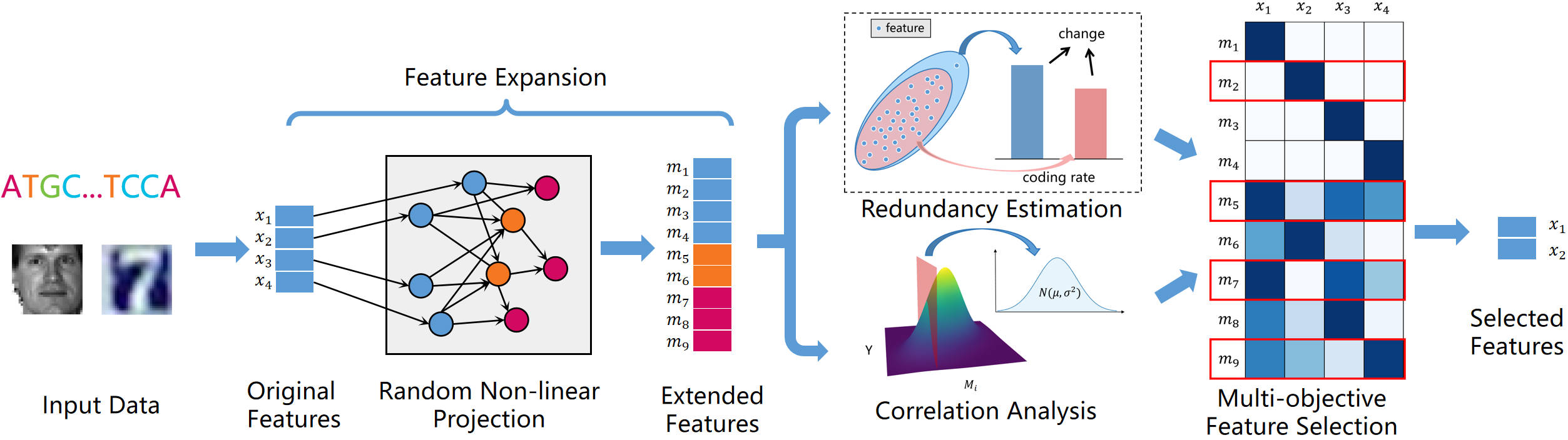
Figure 1: The pipe-line of EasyFS

2 Related Works

Supervised feature selection methods can be divided into model-aware and model-free methods roughly, based on whether there is a need to explicitly define the downstream learner.

In particular, the model-aware methods include the wrapper and embedded approaches according to (Zebari et al., 2020). The wrapper methods treat the learner as a black box. During each selection iteration, a specified number of features are selected and replaced based on the evaluation metrics provided by the downstream learner, so as to test and identify a better feature subset. E.g. HGEFS(Xue et al., 2018) performed feature selection by combining a genetic algorithm with the Extreme Learning Machine (ELM). The Ant Colony Optimization (ACO) has also been used for feature selection in image processing (Chen et al., 2013). All of above methods rely on the running of the downstream predictor, which makes the feature selection procedure time-consuming. Additionally, re-learning of the optimized features is usually required when the downstream learning models are changed, and these methods are prone to overfitting (Gan & Zhang, 2021).

The embedded approaches are another types of model-aware methods, which integrate the feature selection process into the training of the downstream learner. In particular, the EXtreme Gradient Boosting (XGB) (Chen & Guestrin, 2016) and Random Forest (RF)(Díaz-Uriarte & Alvarez de Andrés, 2006) are two commonly used embedded feature selection algorithms based on decision trees. Lasso(Tibshirani, 1996) utilized L1 regularization for input parameter sparsity. They assess the importance of each feature by evaluating its role and frequency of use at splitting decision points. Lasso(Tibshirani, 1996) utilized L1 regularization for input parameter sparsity. Recently, deep learning has gained widespread attention, and an increasing number of studies have focused on using neural networks for embedded feature selection. E.g. DFS (Li et al., 2016) added a sparse connection layer to the input of a multi-layer perceptron (MLP) to learn nonlinear relationships between features through deep connections. LassoNet (Lemhadri et al., 2021) employed skip connections and L1 regularization to implement feature ignoring. AEFS (Han et al., 2018) jointly learned a self-representation autoencoder model and the importance weights of each feature. Wojtas et al.(Wojtas & Chen, 2020) employed a joint training approach with two neural networks and incorporated a random local search process into learning to generate optimal feature subset. STG(Yamada et al., 2020) introduced random gates to the input layer of neural networks, offering theoretical insights of the feature selection procedure based on approximating of Bernoulli distribution. COMPFS(Imrie et al., 2022) proposed the group-wise feature selection using neural networks to identify sparse groups with minimal overlap. TSFS (Mirzaei et al., 2020) presented a teacher-student framework based feature selection method, which employed a teacher network to learn the optimal representation of low-dimensional data and utilized a student network for feature selection. CD-LSR(Xu et al., 2023) transforms the original problem into solving for a discrete selection matrix and utilizes the coordinate descent (CD) method for solving, to achieve sparse learning.

Different from above model-aware methods, the model-free feature selection is independent of the downstream learning algorithm, and ranks the features according to their statistical properties such as mutual information, correlation coefficient, variance, etc. As a typical model-free method, ReliefF (Robnik-Šikonja & Kononenko, 2003b) measured the importance of feature by comparing the feature differences of instances within and between classes. The Fisher Score(Gu et al., 2012) tried another way to measure the importance of feature by calculating the ratio of between-class mean variance to within-class variance. However, it is limited to classification problems. Some research based on mutual information (MRMR (Peng et al., 2005), CIFE(Lin & Tang, 2006) and DISR(Meyer & Bontempi, 2006)) aimed to minimize redundancy within feature subsets while maximizing relevance with the target. Nevertheless, the calculation of mutual information usually incurs a high computational cost, and does not inherently support continuous features. MIRFFS.(Hancer et al., 2018) adopted the differential evolution to address both single-objective and multi-objective problems. Inf-FS (Roffo et al., 2020) treated potential feature subsets as paths on a graph, based on which features were ranked and screened. ManiFeSt(Cohen et al., 2023) proposed a filter feature selection method based on manifold learning and Riemannian geometry.

3 METHODOLOGY

The pipeline of EasyFS is shown in Fig. 1, which contains four basic modules: 1) Feature Expansion through the random projecting network which aims to introduce non-linear combination of original features; 2) Correlation Analysis between the expanded features and downstream tasks based on conditional covariance; 3) Redundancy Estimation of the features based on the code rate of the feature matrix; 4)Multi-objective Feature Selection which aims to select most correlated and less redundant features. The detail of the design will be presented after the formal problem definition in the following sections.

3.1 Problem Formulation

The procedure of feature selection can be formalized as follows. Given a supervised dataset with the input $X\in\mathbb{R}^{d\times n}$, $d$ is the number of features and $n$ is the number of samples. $x_{i,j}$ represents the $i$-th feature of the $j$-th sample, and $X_{i}$ denotes the $i$-th feature across all samples. For the single objective regression problems, the labels are denoted as $Y\in\mathbb{R}^{n}$, representing continuous variables. For the classification problems, the labels are $Y\in\mathbb{R}^{n\times c}$, representing discrete variables. We use $S\subseteq\{1,2,\dots,d\}$ to represent the indices of the feature subset. The goal of feature selection is to find a feature subset $X_{S}=\{X_{i}:i\in S\}$ such that $\mathcal{L}(f_{\theta}(X_{s}),Y)$ is minimized as much as possible. Here, $\mathcal{L}$ is the loss function, and $f_{\theta}(.)$ is the downstream model.

3.2 Feature Expansion Via Random Projecting

Features in high-dimensional feature space of real-world systems tend to be non-independent, and learning the non-linear combination of the features may achieve significantly better performance than the classical linear models as verified by the fast developing deep neural networks. Thus evaluating the significance of the non-linear feature combinations can help to discover potentially more useful features. However, in the model-free feature selection framework, since the downstream learning model is unknown, we have no idea about how the features will be combined in the future. To exploit the potential of possible combinations of features, we propose a lightweight Random Non-linear Projection network, namely RNP for short, to achieve random non-linear combinations of features.

RNP adopts the randomly connected network like the reservoir model (Jaeger, 2002), which aims to capture the non-linear features from input time-series. As illustrated in Fig. 1, there are three types of nodes in the network: the input nodes, hidden nodes and enhancement nodes. The input nodes are densely connected to the hidden nodes, while the enhancement nodes is sparsely connected to other nodes. The adjacency matrix of the network is $W\in\mathbb{R}^{p\times p}$ where $p$ indicates the size of the network, initialized randomly using the standard normal distribution. The input feature vector $X\in\mathbb{R}^{d}$ is fed into the network, and propagated in the network for multiple rounds to achieve non-linear fusion of the features. $I_{t}\in\mathbb{R}^{p}$ denotes the signals transmitted on each node in the $t^{th}$ round of propagation. Initially $I_{0}=[X\quad 0]$, where the signals of the first $d$ input nodes are set as the input feature vector $X$, and the ones of left nodes are set as zero. $h_{t}\in\mathbb{R}^{p}$ represents the internal state of each node in the $t^{th}$ round. $h_{0}=0$. $M_{t}\in\mathbb{R}^{p}$ indicates the output signal of each node, which is calculated through the non-linear propagation procedure as follows:

$$I_{t+1}=ReLU(h_{t}+WI_{t})$$ (1)

$$h_{t+1}=h_{t}+WI_{t}-I_{t+1}$$ (2)

$$M_{t+1}=M_{t}+I_{t+1}$$ (3)

The ReLU activation function in Eq. 1 is used to introduce the non-linear transformation of the signals. The output signals $M_{t}$ at the final time step, is used as the non-linear expanded features with $p$ dimension, which is defined as $\hat{M}$:

$$\hat{M}=M_{T}$$ (4)

Here $T$ is the number of propagation rounds.

3.3 Correlation Analysis

To measure the significance of each expanded feature $\hat{M}$, we calculate the correlation between the features and the downstream classification/regression tasks. In particular, for the regression problems, Inspired by (Chen et al., 2017), we use the conditional covariance to characterize the correlation. The joint distribution of the $i^{th}$ feature $\hat{M_{i}}$ and the regression target Y can be fitted as a a two-dimensional Gaussian distribution as follows:

$$Y,\hat{M_{i}}\sim N(\mu_{i},\Sigma_{i})$$ (5)

$$\mu_{i}=\left(\begin{array}[]{l}\mu_{Y}\\ \mu_{\hat{M_{i}}}\end{array}\right)\Sigma_{i}=\begin{pmatrix}\sigma_{Y\hat{M_{i}}}&\sigma_{YY}\phantom{{}_{iii}}\\ \sigma_{\hat{M_{i}}Y}&\sigma_{\hat{M_{i}}\hat{M_{i}}}\end{pmatrix}$$ (6)

The conditional distribution of a two-dimensional Gaussian distribution is also a Gaussian distribution.

$$Y|\hat{M_{i}}\sim N(\mu_{Y}+\sigma_{Y\hat{M_{i}}}\sigma_{\hat{M_{i}}\hat{M_{i}}}^{-1}(\hat{M_{i}}-\mu_{\hat{M_{i}}}),\sigma_{Y|\hat{M_{i}}})$$ (7)

The conditional variance $\sigma_{Y|M_{i}}$ is:

$$\sigma_{Y|M_{i}}=\sigma_{YY}-\sigma_{Y\hat{M_{i}}}\sigma_{\hat{M_{i}}\hat{M_{i}}}^{-1}\sigma_{\hat{M_{i}}Y}$$ (8)

Smaller $\sigma_{Y|\hat{M_{i}}}$ indicates higher correlation between $\hat{M_{i}}$ and $Y$, so the correlation score of the feature $\hat{M_{i}}$ can be defined as:

$$L_{i}=\sigma_{Y|\hat{M_{i}}}$$ (9)

For classification problems, we directly use the standard deviation of the within-class features to measure the correlation between the feature $\hat{M_{i}}$ and the $k^{th}$ class:

$$L_{i}^{k}=\sqrt{Var(\{\hat{M}_{i,j}|Y_{j}=k\})}$$ (10)

Here $\hat{M}_{i,j}$ indicates the $i^{th}$ expanded feature of the $j^{th}$ instance. Smaller $L_{i}^{k}$ indicates the higher correlation between $\hat{M_{i}}$ and the $k^{th}$ class.

3.4 Redundancy Estimation

One important goal of feature selection is to filter out the redundant features. Mutual information has been broadly used as redundancy measurement by existing feature selection methods (Peng et al., 2005)(Ross, 2014). However, the calculation of mutual information for continuous features are timing costly. In this paper, we propose an efficient redundancy metric based on the coding rate (average coding length) of the feature matrix, which is firstly used by $MCR^{2}$ (Yu et al., 2020) to measure the compactness of the features. Given the feature matrix $\hat{M}\in\mathbb{R}^{p\times n}$, the coding rate (Yu et al., 2020) can be calculated as follows:

$$R(\boldsymbol{\hat{M}},\epsilon)=\frac{1}{2}\log\operatorname{det}\left(\boldsymbol{I}+\frac{p}{n\epsilon^{2}}\boldsymbol{\hat{M}}^{\top}\boldsymbol{\hat{M}}\right)$$ (11)

Here $\epsilon$ is constant to control the magnitude of coding precision. We represent the redundancy of a feature by examining the variation of the coding rate when the feature is removed from the instances. For the $i^{th}$ feature, the variation of the code rate is:

$$Q_{i}=R(\hat{M},\epsilon)-R(\hat{M}_{\ominus i},\epsilon)$$ (12)

Here $\hat{M}_{\ominus i}$ indicates the modified feature matrix of $\hat{M}$ by removing the $i^{th}$ row, which is corresponding to the $i^{th}$ feature. Larger $Q_{i}$ indicates less redundancy of the $i^{th}$ feature.

The calculation of Eq. 12 has to be run for each feature, so the measurement is costly for high dimensional feature space. To simplify the calculation of, we rewrite the measurement in a compact matrix form in Eq. 13.

$$\begin{split}Q&=\{Q_{1},Q_{2},...,Q_{p}\}\\ &=R(\boldsymbol{\hat{M}},\varepsilon)-\frac{1}{2}log(diag(det(G)G^{-1}))\\ \end{split}$$ (13)

$$G=\boldsymbol{I}+\frac{p-1}{n\epsilon^{2}}\boldsymbol{\hat{M}}^{\top}\boldsymbol{\hat{M}}$$ (14)

The detailed proof of Eq. 13 is provided in the Appendix A.

Meanwhile, for the classification problems, the redundancy measurement $Q_{i}^{k}$ is calculated for the $k^{th}$ class based on the feature matrix of the instances belonging to the class.

3.5 Multi-objective Feature Selection

In order to select most correlated and less redundant features, we combine the correlation measurement $L_{i}$ and $Q_{i}$ of the $i^{th}$ feature to evaluate its importance in the regression task:

$$S_{i}=L_{i}-\lambda_{1}Q_{i}(1-e^{-Q_{i}})$$ (15)

Where $\lambda_{1}$ is a positive constant used to control the fusion ratio. $L_{i}$ and $Q_{i}$ are both pre-processed with min-max normalization before fusion. To emphasize non-redundant features, we add a non-linear weight to the redundancy index, which is defined as $1-e^{-Q_{i}}$. $S_{i}$ can be used to evaluate the importance of the extended feature $\hat{M}_{i}$, where smaller $S_{i}$ indicates higher correlation and lower redundancy.

To perform the feature selection on the original features, we still need to obtain the influence of the original features on the extended features and reflect the importance of high-dimensional features back to the original features. According to Eq. 3, the extended feature is the accumulation of the non-linear propagation of the original feature. The support of original feature $X_{j}(j\leq d)$ on the extended feature $\hat{M}_{i}(i\leq q)$ can be defined based on the propagation matrix $W$ as follows:

$$E_{ij}=|(W+I)^{T}_{ij}|$$ (16)

Here $|\cdot|$ indicates the absolute value function.

After sorting $S_{i}$ for all expanded features in ascending order, we select the top $r\%$ extended features and calculate the importance of the $j^{th}$ original feature as the support of feature on the selected important extended features:

$$H_{j}={\textstyle{}\sum_{i\in Top\_r(\{S_{i}\})}}E_{ij}$$ (17)

Here $Top\_r(\cdot)$ indicates the index of the top $r\%$ values in $\{S_{i}|i\leq q\}$. Higher $H_{j}$ indicates high importance of the feature $X_{j}$.

By combining both of the correlation and redundancy measurements, the multi-object feature selection can be done by ranking the original features according to $H_{j}$ in descendant order. For the classification tasks, the similar evaluation can be done for feature selection, the detail of which is shown in the Appendix B. The full algorithm of the EasyFS covering the whole procedure of feature selection on classification/regression is detailed in the Appendix C.

Table 1: Regression task datasets

Dataset	#Samples	#Feature
COIL-2000	5822	85
CSD-1000R	500	100
SLICE	53500	385
SML	4137	26
SoyNAM-height	5128	4236
SoyNAM-oil	5128	4236
SoyNAM-moisture	5128	4236
SoyNAM-protein	5128	4236
Wheat599-env1	599	1279
Wheat599-env2	599	1279
Wheat599-env3	599	1279
Wheat599-env4	599	1279

4 Experiment

4.1 Experimental Configurations

Datasets.  We validate our method on 12 regression datasets and 9 classification datasets as shown in Table 1 and Table 2. Readers can refer to Appendix D for detailed description of the datasets.

Evaluation metrics. For the regression problem, in order to eliminate the diversity of the value range in different datasets, the Normalized Mean Square Error Loss NMSE is used as an evaluation metric like (Rustam et al., 2019):

$$NMSE=\frac{{\textstyle\sum_{n}^{i=1}|y_{i}-\hat{y_{i}}|^{2}}}{\sum_{n}^{i=1}|y_{i}-\hat{y}|^{2}}$$ (18)

Here $\hat{y_{i}}$ is the predicted label, $y_{i}$ is the true label, and $\hat{y}$ denotes the mean of the true labels. Meanwhile, for the classification tasks, the average classification accuracy (ACC) based on k-fold cross-validation is adopted as the evaluation metric like (Imrie et al., 2022).

Experimental setup. For each dataset, 5-fold cross-validation is conducted. For regression tasks, the Support Vector Machine Regression (SVR) with an RBF kernel is adopted as the downstream learner. For classification tasks, the Support Vector Machine Classification (SVM) with a linear kernel is used as the downstream learner. The parameters of the learners are set to their default values in Scikit-learn (Pedregosa et al., 2011). All experiments are conducted using a CPU running at 2.20 GHz and a Nvidia 1080ti GPU.

Baselines. Our proposed EasyFS is compared with several popular feature selection methods, including the model-free and model-aware algorithm as follows.

Table 2: Classification task datasets

Dataset	#Samples	#Feature	#Classes
COIL20	1440	1024	20
ORL	400	1024	40
PIE-05	3332	1024	68
TOX	171	5748	4
UMIST	575	1024	20
SVHN	99289	3072	10
warpAR10P	130	2400	10
YALE	165	1024	15
YALEB	2414	1024	38

1) Model-aware Methods

• spFSR(Akman et al., 2023) is a recently proposed method based on Simultaneous Perturbation Stochastic Approximation (SPSA) with Barzilai and Borwein (BB) non-monotone gains.

• The stochastic gate (STG) (Yamada et al., 2020) introduces a stochastic gating mechanism at the input layer of neural networks to select important features by gradient descent.

• Lassonet (Lemhadri et al., 2021) integrates the skip connections into ResNet (He et al., 2016) and utilizes L1 regularization to achieve feature selection.

• EXtreme Gradient Boosting (XGB) (Chen & Guestrin, 2016) and Random Forests (RF) (Díaz-Uriarte & Alvarez de Andrés, 2006) are commonly used ensemble learning algorithms based on the tree structure and also serve as embedded feature selection methods.

• LASSO (Tibshirani, 1996; Muthukrishnan & Rohini, 2016) is a classic embedded feature selection algorithm that combines regression with regularization to impose weight constraints.

2) Model-free Methods

• SPEC (Zhao & Liu, 2007) is based on spectral theory and assesses the importance of features by analyzing the spectral properties of the data.

• ReliefF (Robnik-Šikonja & Kononenko, 2003a) evaluates the importance of features by estimating their ability to distinguish neighboring samples. However, it is only applicable to classification problems.

• Fisher Score (Gu et al., 2012) is a statistical-based method for classification problems based on the measurement of the intra-class and inter-class differences.

• MCFS (Cai et al., 2010) integrates manifold learning and L1-regularized models to identify important features.

• PPMCC algorithm (Hall, 1999) utilizes the Pearson correlation coefficient to rank the importance of features.

• MI algorithm (Estévez et al., 2009) uses the mutual information between features and target variables to measure the feature importance.

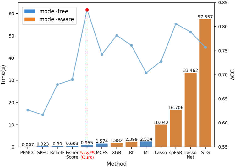
Figure 2: Runtime (by column) and Accuracy (by curve) on the YALE dataset

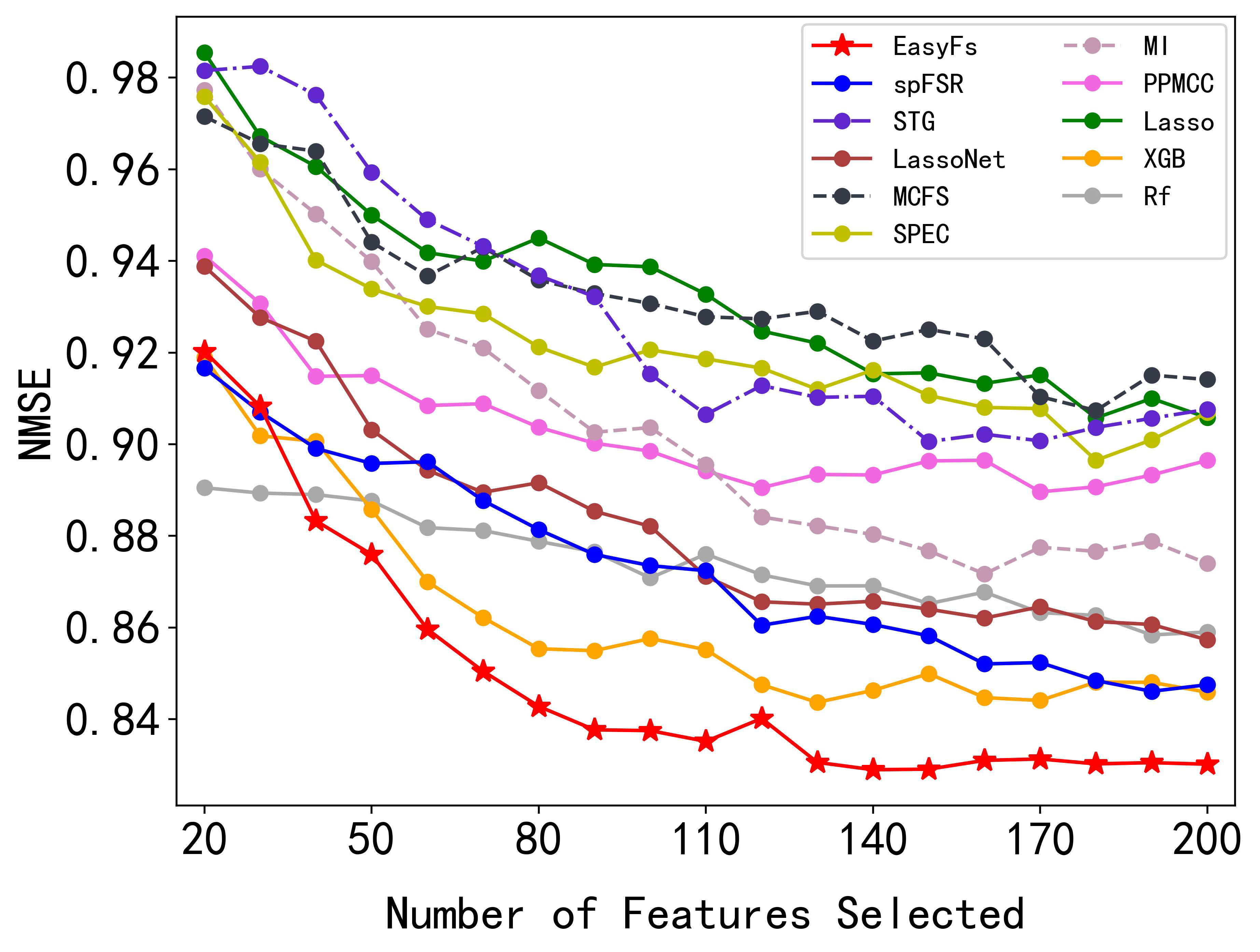
Figure 3: NMSE on the regression dataset SoyNAM-height. (Smaller NMSE is better)

Table 3: Regression Results of NMSE (Smaller is better)

[b] Dataset N_s spFSR LassoNet STG Rf XGB Lasso PPMCC MI SPEC MCFS EasyFS (Ours) COIL-2000 10 0.0125 0.0145 0.7610 0.0122 0.0121 0.0120 0.0127 0.0120 0.0122 0.7645 0.0115 ↓4.1% 20 0.0122 0.0144 0.7393 0.0118 0.0118 0.0116 0.0121 0.0119 0.0121 0.6812 0.0115 ↓1.3% CSD-1000R 10 0.8027 0.8251 0.8647 0.7731 0.7818 0.7346 0.7790 0.8280 0.8103 0.8184 0.6782 ↓7.7% 20 0.7478 0.7611 0.7890 0.6707 0.7482 0.6502 0.7284 0.7610 0.8056 0.6738 0.6163 ↓5.2% SLICE 10 0.5634 0.5335 0.6482 0.5561 0.5664 0.4217 0.6906 0.8730 0.9444 0.6110 0.4047 ↓4.0% 20 0.4245 0.4659 0.5107 0.4845 0.4216 0.3540 0.6866 0.8228 0.8310 0.4974 0.3379 ↓4.5% SML 10 0.0635 0.0446 0.4834 0.0414 0.0427 0.0411 0.0383 0.0410 0.0592 0.1090 0.0373 ↓2.6% 20 0.0365 0.0369 0.0431 0.0353 0.0350 0.0350 0.0359 0.0353 0.0390 0.0351 0.0350 ↓0.1% SoyNAM-height 50 0.8958 0.9031 0.9593 0.8876 0.8858 0.9500 0.9150 0.9399 0.9339 0.9441 0.8760 ↓1.1% 150 0.8582 0.8640 0.9006 0.8652 0.8499 0.9156 0.8964 0.8768 0.9106 0.9251 0.8291 ↓2.5% SoyNAM-moisture 50 0.8893 0.9201 1.0024 0.8841 0.9119 0.9956 0.8889 0.9313 0.9757 0.9834 0.8790 ↓0.6% 150 0.8788 0.9054 0.9908 0.8703 0.8844 0.9744 0.8776 0.9091 0.9448 0.9449 0.8508 ↓2.2% SoyNAM-oil 50 0.9392 0.9057 0.9835 0.9039 0.9104 0.9781 0.9225 0.9859 0.9551 0.9508 0.8872 ↓1.8% 150 0.9019 0.8897 0.9651 0.8779 0.8733 0.9397 0.9174 0.9495 0.9301 0.9450 0.8694 ↓0.5% SoyNAM-protein 50 0.8914 0.9586 0.9608 0.8836 0.8906 0.9467 0.9122 0.9467 0.9388 0.9379 0.8754 ↓0.9% 150 0.8771 0.9166 0.9715 0.8820 0.8692 0.9179 0.9234 0.9266 0.9050 0.9277 0.8523 ↓1.9% wheat599-env1 50 0.8135 0.8225 0.7653 0.8506 0.8062 0.8129 0.8378 0.9054 0.9072 0.8000 0.7363 ↓3.8% 150 0.7568 0.7604 0.7642 0.7779 0.7514 0.7619 0.7586 0.7766 0.8254 0.7590 0.6694 ↓10.9% wheat599-env2 50 0.8983 0.9417 0.9094 0.9285 0.9236 1.0162 0.9806 0.9192 0.9641 1.0003 0.8462 ↓5.8% 150 0.8235 0.8461 0.8719 0.8300 0.8392 0.8739 0.8576 0.8559 0.9923 0.8584 0.7941 ↓3.6% wheat599-env3 50 0.9282 0.9470 0.9415 0.9569 0.9691 0.9914 0.9814 1.0327 1.0037 1.0136 0.8842 ↓4.7% 150 0.8912 0.9237 0.8916 0.8904 0.9364 0.9233 0.9101 0.9546 0.9919 0.9148 0.8552 ↓3.9% wheat599-env4 50 0.8739 0.8962 0.8245 0.8425 0.8710 0.8578 0.9062 0.8566 0.9823 0.9280 0.8076 ↓2.0% 150 0.8238 0.8193 0.8193 0.8407 0.8357 0.8514 0.8487 0.8146 0.9742 0.8900 0.7646 ↓6.1%

• $N_{s}$ represents the number of selected features, and the best performance for the subset selection problem is highlighted in bold, while the second-best performance is indicated with an underscore.

Table 4: Classification Results of ACC (Larger is better)

[b] Dataset N_s spFSR Lasso Net STG Rf XGB Lasso PPMCC MI ReliefF SPEC MCFS Fisher Score EasyFS (Ours) COIL20 30 0.916 0.876 0.790 0.829 0.924 0.849 0.598 0.756 0.744 0.664 0.827 0.741 0.944 ↑2.2% 50 0.951 0.942 0.872 0.910 0.964 0.915 0.697 0.824 0.815 0.775 0.912 0.835 0.981 ↑1.8% ORL 30 0.882 0.823 0.795 0.812 0.823 0.815 0.615 0.642 0.688 0.557 0.805 0.765 0.893 ↑1.2% 50 0.925 0.893 0.893 0.905 0.907 0.887 0.705 0.735 0.767 0.725 0.878 0.838 0.950 ↑2.7% PIE-05 30 0.944 0.905 0.943 0.824 0.901 0.914 0.857 0.787 0.828 0.750 0.881 0.637 0.944 ↑0.0% 50 0.970 0.952 0.969 0.903 0.959 0.964 0.925 0.851 0.902 0.899 0.947 0.774 0.977 ↑0.7% TOX 30 0.748 0.830 0.656 0.714 0.743 0.731 0.690 0.749 0.649 0.579 0.696 0.626 0.860 ↑3.6% 50 0.778 0.860 0.778 0.784 0.789 0.696 0.749 0.772 0.678 0.708 0.732 0.684 0.895 ↑4.1% UMIST 30 0.962 0.941 0.934 0.927 0.972 0.937 0.586 0.788 0.816 0.798 0.901 0.917 0.963 ↓0.9% 50 0.976 0.962 0.950 0.965 0.977 0.970 0.732 0.857 0.894 0.890 0.970 0.958 0.979 ↑0.2% warpAR10P 30 0.892 0.869 0.823 0.877 0.908 0.815 0.638 0.815 0.800 0.562 0.831 0.862 0.946 ↑4.2% 50 0.946 0.908 0.846 0.900 0.962 0.823 0.769 0.862 0.815 0.569 0.908 0.923 0.985 ↑2.4% YALE 30 0.675 0.636 0.600 0.588 0.600 0.430 0.358 0.576 0.436 0.352 0.576 0.594 0.697 ↑3.3% 50 0.775 0.715 0.648 0.667 0.709 0.564 0.418 0.624 0.558 0.418 0.667 0.576 0.818 ↑5.5% YALEB 30 0.833 0.788 0.826 0.797 0.687 0.623 0.718 0.764 0.643 0.664 0.628 0.579 0.850 ↑2.0% 50 0.913 0.889 0.911 0.901 0.847 0.766 0.834 0.876 0.805 0.814 0.806 0.708 0.920 ↑0.8% SVHN 30 0.204 0.200 0.194 0.198 0.201 0.200 0.196 0.200 0.199 0.194 0.193 0.198 0.215 ↑5.4% 50 0.212 0.206 0.193 0.201 0.205 0.203 0.196 0.202 0.197 0.193 0.194 0.200 0.224 ↑5.7%

• $N_{s}$ represents the number of selected features, and the best performance for the subset selection problem is highlighted in bold, while the second-best performance is indicated with an underscore.

4.2 Experimental Result

We compare the performance of various feature selection methods on both regression and classification tasks in Tables 4 and 3, where $N_{s}$ represents the number of selected feature subsets. We also depict comparison curves for selected datasets at each step of two typical datasets will highest dimensions in Fig. 4 and Fig. 3. Reader can refer to Appendix F for the full results on all datasets. The results indicate that our proposed EasyFS outperforms the aforementioned feature selection methods in almost all cases. In particular, the superiority of EasyFS over the the second-best method by 5.7% on the SVHN classification dataset, and 10.9% On the wheat599-env1 regression dataset. For other feature selection algorithms, spFSR, STG, and XGB exhibit strong performance in classification tasks, while Lasso and spFSR perform well in regression tasks. Furthermore, we adding the visualization analysis of all methods to verify the effectivess of the model in the Appendix G.

Figure 4: ACC on the classification dataset Tox. (Higher ACC is better)

Additionally, we compared the runtime required by different algorithms to select the top 5% of features during feature selection on the YALE dataset in Fig. 2. It can be observed that the model-free algorithms such as ReliefF, PPMCC, and Fisher Score exhibit the fastest execution times, but have relatively much worse performance of the downstream classification task. In contrast, algorithms based on gradient descent, such as STG, LassoNet, and Lasso, have better classification performance, but require much more time, e.g. STG even taking 146 times longer than the ReliefF algorithm. Our method EasyFS have the highest classification performance while saving more than 94% time compared to the latest model-aware method spFSR.

Ablation. Based on the Wheat599-env1 dataset, we conducted experiments to test the effectiveness of three important modules of DeepFS: Random Non-linear Projection (RNP), Redundancy Estimation (RE), and Correlation Analysis (CA). As shown in Table 5, adding the RNP structure reduces the error by 10.87%, while building the RNP and its propagation process is also the main part of algorithm time consumption. The addition of CR reduced the error by 3.1% with a relatively minor impact on the running speed.

Table 5: Ablation Experiment

Dataset	RNP	CR	CA	Time(s)	NMSE
Wheat599 -env1	$\surd$	$\surd$	$\surd$	1.324	0.713
	$\surd$	$\times$	$\surd$	1.031	0.746
	$\times$	$\surd$	$\surd$	0.128	0.811
	$\times$	$\times$	$\surd$	0.007	0.837

Parameter Analysis. In EasyFS, the size of the Random Non-linear Projecting Network (RNP) and the hyperparameter $r$ for selecting the top $r\%$ high-dimensional features can influence the experimental results. We varied the feature range expanded by RNP from $\{0,300,...,1500\}$ and $r$ from $\{0.1,0.2,...,0.7\}$, and the experimental results are shown in Fig. 5. It can be observed that as the RNP size increases, the error rapidly decreases and then stabilizes with small fluctuations. The choice of $r$ needs to be within a reasonable range because selecting too few or too many high-dimensional features can lead to an increase of error. Selecting too many features introduces more unrelated features, while selecting too few may not utilize enough information of non-linear combinations of features.

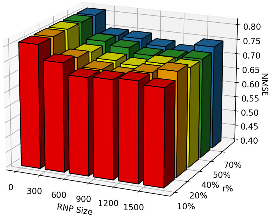
Figure 5: Parameter Analysis

5 conclusion

In this paper, we propose a high-performance model-free feature selection method via elastic transformation of features, namely EasyFS, to achieve the goals of effectiveness, efficiency and flexibility. EasyFS utilizes a Random Non-linear Projection Network to expanding the feature space and calculate the correlation of high-dimensional features. Meanwhile, a novel redundancy measurement based on coding rate is proposed to decrease the feature dimension efficiently. Comprehensive experiments on both classification and regression tasks, which are conducted based on 21 real-world datasets, show the superior performance of EasyFS on both of the precision of downstream tasks and the timing cost compared with state-of-the-art methods.

In the future, we will extend EasyFS to further support the feature selection in the multi-modal use cases.

Appendix A Coding Redundancy Matrix operation formula derivation

The spatial encoding rate formula for a certain batch of samples.

$$R(\boldsymbol{M},\epsilon)=\frac{1}{2}\log\operatorname{det}\left(\boldsymbol{I}+\frac{p}{n\epsilon^{2}}\boldsymbol{M}^{\top}\boldsymbol{M}\right)\in R^{p\times p}$$ (19)

If one column (a one-dimensional feature) is removed from M, get $M_{i^{\prime}}=\{M_{j}\mid j\in\{0,1,\ldots,l\},j\neq i\}$, it can be obtained that

$$R(\boldsymbol{M_{i^{\prime}}},\epsilon)=\frac{1}{2}\log\operatorname{det}\left(\boldsymbol{I}+\frac{p}{n\epsilon^{2}}\boldsymbol{M_{i^{\prime}}}^{\top}\boldsymbol{M_{i^{\prime}}}\right)\in R^{(p-1)\times(p-1)}$$ (20)

At this point, let

$$R(\boldsymbol{M_{i^{\prime}}},\epsilon)=\frac{1}{2}logdet(G_{i^{\prime}})$$ (21)

$$G=\boldsymbol{I}+\frac{p-1}{n\epsilon^{2}}\boldsymbol{M}^{\top}\boldsymbol{M}\in R^{p\times p}$$ (22)

Then, $G_{i^{\prime}}$ is exactly the value of $G$ after removing the i-th row and the i-th column.

$$G=\boldsymbol{I}+\frac{p-1}{n\epsilon^{2}}\boldsymbol{M}^{\top}\boldsymbol{M}\in R^{p\times p}$$ (23)

We want to calculate the determinant of $G_{i^{\prime}}$ for each iteration over i, which is ${det(G_{1^{\prime}}),det(G_{2^{\prime}}),...,det(G_{p^{\prime}})}$, and express it in matrix form.

$$\begin{bmatrix}det(G_{1^{\prime}})&0&\dots&0\\ 0&det(G_{1^{\prime}})&\dots&0\\ \vdots&\vdots&\ddots&\vdots\\ 0&0&\dots&det(G_{p^{\prime}})\\ \end{bmatrix}$$ (24)

Then, according to the definition of the adjugate matrix, these terms exactly correspond to the diagonal of the adjugate matrix of G, which is $diag(adj(G))$. The adjugate matrix can be calculated through the inverse of the matrix and its determinant as $adj(G)=det(G)G^{-1}$.

so

$$\{det(G_{1^{\prime}}),det(G_{2^{\prime}}),...,det(G_{p^{\prime}})\}=diag(det(G)G^{-1})$$ (25)

$$\{R(\boldsymbol{M_{1^{\prime}}},\epsilon),R(\boldsymbol{M_{2^{\prime}}},\epsilon),...,R(\boldsymbol{M_{n^{\prime}}},\epsilon)\}=\frac{1}{2}log(diag(det(G)G^{-1}))$$ (26)

$$\begin{split}Q&=\{Q_{1},Q_{2},....,Q_{n}\}\\ &=R(M,\epsilon)-\{R(\boldsymbol{M_{1^{\prime}}},\epsilon),R(\boldsymbol{M_{2^{\prime}}},\epsilon),...,R(\boldsymbol{M_{n^{\prime}}},\epsilon)\}\\ &=R(M,\epsilon)-\frac{1}{2}log(diag(det(G)G^{-1}))\end{split}$$ (27)

Appendix B Importance Evaluation of Features in the Classification Tasks

For the classification tasks, the importance of the $i^{th}$ extended features for the $k^{th}$ class can be defined similar with Eq. 15:

$$S_{i}^{k}=L_{i}^{k}-\lambda_{1}Q_{i}^{k}(1-e^{-Q_{i}^{k}})$$ (28)

Similar with Eq. 17, the importance of the $j^{th}$ original feature on the $k^{th}$ class can be defined as:

$$H_{j}^{k}={\textstyle{}\sum_{i\in Top\_r(\{S_{i}^{k}\})}}E_{ij}$$ (29)

Inspired by Fisher Score(Gu et al., 2012), Laplacian Scoree(He et al., 2005), and ReliefF(Robnik-Šikonja & Kononenko, 2003b), we further extend Eq. 29 by emphasize features with large inter-class variation as follows:

$$H_{i}^{k}={\textstyle{}\sum_{i\in Top\_r(\{S_{i}^{k}\})}}(\sigma_{i}^{\mu}+\lambda_{2}\sigma_{i}^{\sigma})E_{ij}$$ (30)

Here $\mu_{i}^{k}$ and $\sigma_{i}^{k}$ represent the mean and variance of the $i$-th feature within class $k$. $\sigma_{i}^{\mu}$ represent the variance of the inter-class means and $\sigma_{i}^{\sigma}$ to represent the variance of inter-class variances for the i-th feature.

The importance of the $j^{th}$ original feature is calculated as follows in the end:

$$H_{i}=\sum_{k=1}^{c}H_{i}^{k}$$ (31)

Appendix C Full Algorithm of EasyFS

Algorithm 1 EasyFS Algorithm.

0:  dataset$\{X,Y\}$; Hyperparameter $\lambda_{1},\lambda_{2},r$; $W$,$T$ for RNP parameter

1:  Calculate $E_{ij}$ by Eq. (16)

2:  Calculate $M$,Mapping features $f:\mathbb{R}^{d}\rightarrow\mathbb{R}^{p}$ via RNP

3:  if Regression Task then

4:     Calculate $G=\boldsymbol{I}+\frac{p-1}{n\epsilon^{2}}\boldsymbol{M}^{\top}\boldsymbol{M}$

5:     Calculate $Q=R(M,\varepsilon)-\frac{1}{2}log(diag(det(G)G^{-1}))$

6:     for i = 1,…,p do

7:        Calculate correlation $L_{i}=\sigma_{Y|M_{i}}=\sigma_{YY}-\sigma_{Y\hat{M_{i}}}\sigma_{\hat{M_{i}}\hat{M_{i}}}^{-1}\sigma_{\hat{M_{i}}Y}$

8:        Calculate $S_{i}=L_{i}-\lambda_{1}Q_{i}(1-e^{-Q_{i}})$

9:        Calculate feature importance $H_{i}$ by Eq. (17)

10:     end for

11:  else if Classification Task then

12:     for k = 1,…,c do

13:        Calculate $G=\boldsymbol{I}+\frac{p-1}{n\epsilon^{2}}\boldsymbol{M^{k}}^{\top}\boldsymbol{M^{k}}$

14:        Calculate $Q^{k}=R(M^{k},\varepsilon)-\frac{1}{2}log(diag(det(G)\allowbreak G^{-1}))$

15:        for i = 1,…,p do

16:           Calculate correlation $L_{i}^{k}$ by Eq. (10)

17:           Calculate $S_{i}^{k}=L_{i}^{k}-\lambda_{1}Q_{i}^{k}(1-e^{-Q_{i}^{k}})$

18:           Calculate $H_{i}^{k}$ by Eq. (30)

19:        end for

20:     end for

21:     Calculate feature importance $H_{i}$ by Eq. (31)

22:  end if

23:  Return rank($H_{i}$)

Appendix D Dataset Configurations

Regression task datasets. We validate our method on both regression and classification datasets. For regression tasks, we use a total of 12 datasets, including 4 single-target regression datasets and derived subsets from 8 multi-target gene expression datasets. Most of these datasets are sourced from the UCI Machine Learning Repository(Frank, 2010) and other publicly available datasets. SoyNAM(Liu et al., 2019) is a gene dataset comprising the genotype-phenotype relationships of 5128 soybean plants. It uses 4236 genes to predict various phenotypic traits of soybeans, including protein content, oil content, moisture content, and height. Each phenotype is treated as a separate prediction target since different genes influence each phenotype differently. Consequently, the dataset is divided into four distinct sub-datasets: SoyNAM-height, SoyNAM-oil, SoyNAM-moisture, and SoyNAM-protein. Wheat599(Wang et al., 2023) is a dataset consisting of 599 historical wheat lines obtained from the International Maize and Wheat Improvement Center (CIMMYT) Global Wheat Program(McLaren et al., 2005). The project involved multiple international wheat experiments, categorizing wheat-growing environments into four main climatic regions. The dataset records the yield of the same wheat genotypes in these four different production environments. Similarly, we treat these four environments as four separate targets, resulting in four sub-datasets: Wheat599-env1, Wheat599-env2, Wheat599-env3, and Wheat599-env4. The COIL-2000(Frank, 2010) dataset comprises information on 5822 customers of an insurance company. It aims to predict the customer type or class based on individual customer attributes such as whether they have received higher education, the number of children they have, income, and so on. SLICE(Frank, 2010) is a medical dataset that contains information from 71 patients and 53,500 CT images, using Histogram describing bone structures and Histogram describing air inclusions to predict Relative location of the image on the axial axis. The SML dataset collects environmental sensor data from rooftop sensors, including parameters such as temperature, humidity, and wind speed. It comprises 4,371 records of environmental sensor data. The CSD-1000R dataset, as described in (Musil et al., 2019), contains atomic environments of C, H, N, and O atoms extracted from the crystal structures of molecular compounds. This dataset is used for predicting their NMR chemical shielding. The number of samples and the number of features for all regression datasets are shown in Table 1.

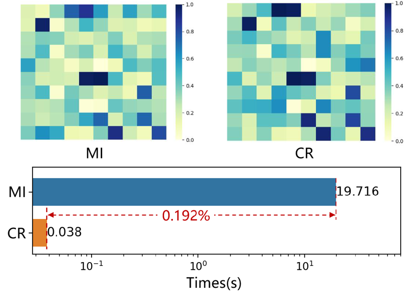
Figure 6: Comparison with mutual information

Classification task datasets. For classification tasks, we conducted experiments on 9 datasets. The COIL20 object recognition dataset(Nene et al., 1996) contains grayscale images of 20 objects captured from different angles. There are 72 images taken for each object, with images taken at 5-degree intervals. The ORL face dataset(Samaria & Harter, 1994), consisting of 400 images from 40 different individuals, was collected under various conditions such as different times, lighting conditions, facial expressions (open eyes/closed eyes, smiling/not smiling), and facial details (with glasses/without glasses). The PIE-05 dataset(Sim et al., 2002) consists of imaging data from 68 volunteers captured under 43 different lighting conditions, with four distinct facial expressions, and across 13 unique poses for each individual.We use the data captured by Camera 05, which comprises a total of 3332 images. UMIST(Graham & Allinson, 1998), warpAR10P(Li et al., 2017), YALE(Khalajzadeh et al., 2014), YALEB(Georghiades et al., 2001) are all face recognition datasets. The TOX dataset(Bolón-Canedo et al., 2014) is a biological dataset that includes 171 samples, each with 5748 genes. It is divided into four categories: non-cancer patients, controlled radiation therapy patients, cancer skin patients, and radiation therapy patients. SVHN (Street View House Numbers)(Netzer et al., 2011) is a digit recognition dataset obtained by cropping images of house numbers from street view scenes. It contains 99,289 color images of digits, each with a resolution of 32x32 pixels. Example of the SVHN dataset as shown in Fig. 9.The number of samples and features for all classification datasets is shown in Table 2.

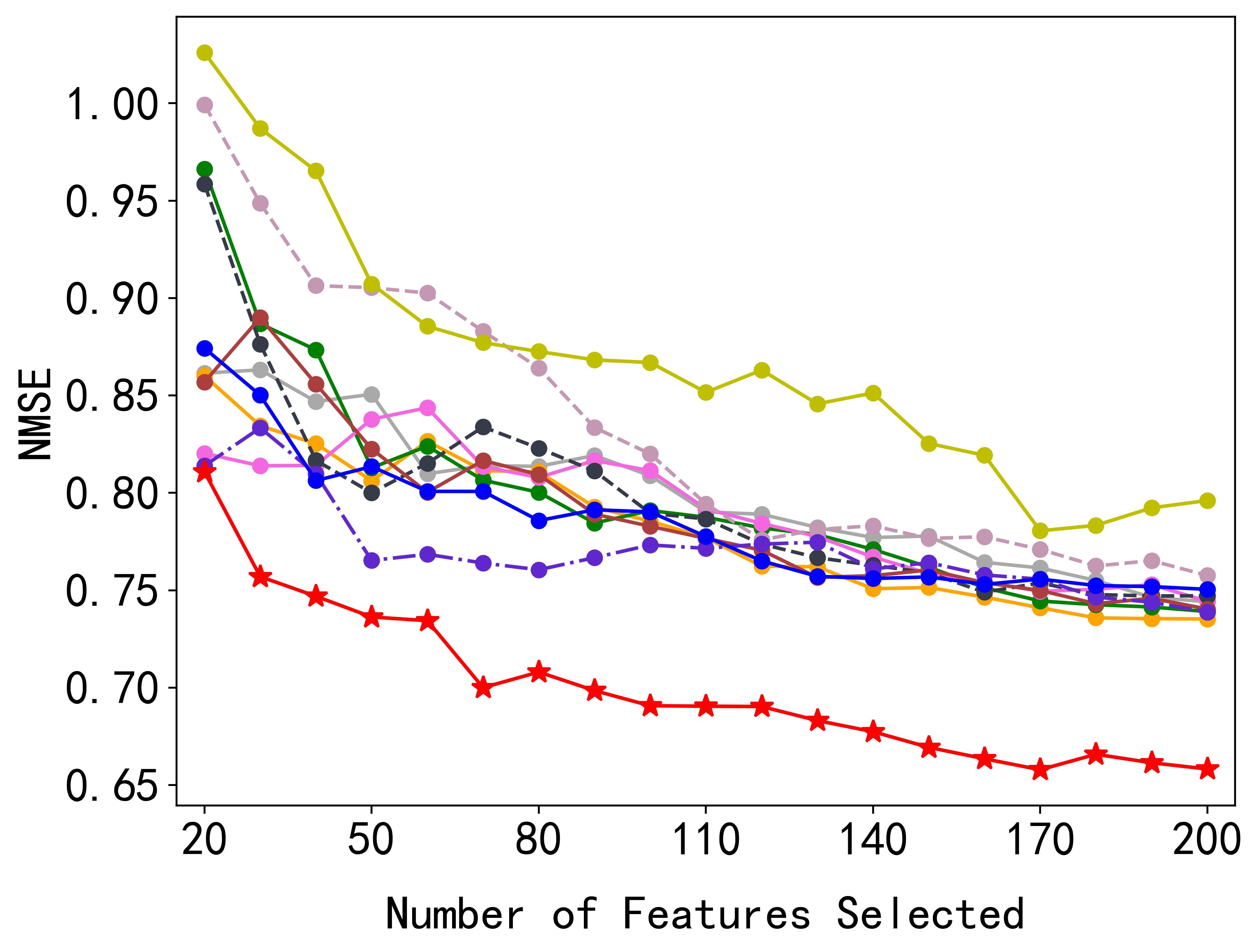
(a) Wheat599-env1

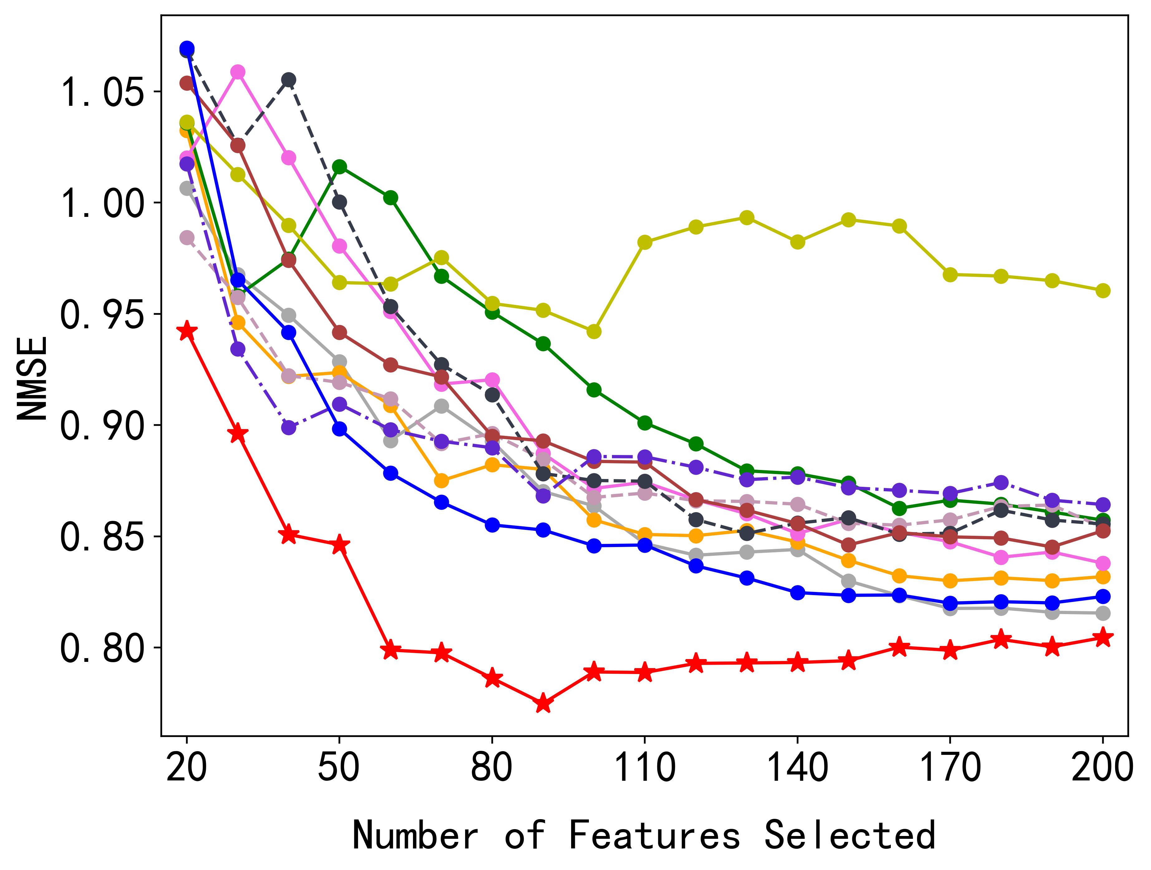
(b) Wheat599-env2

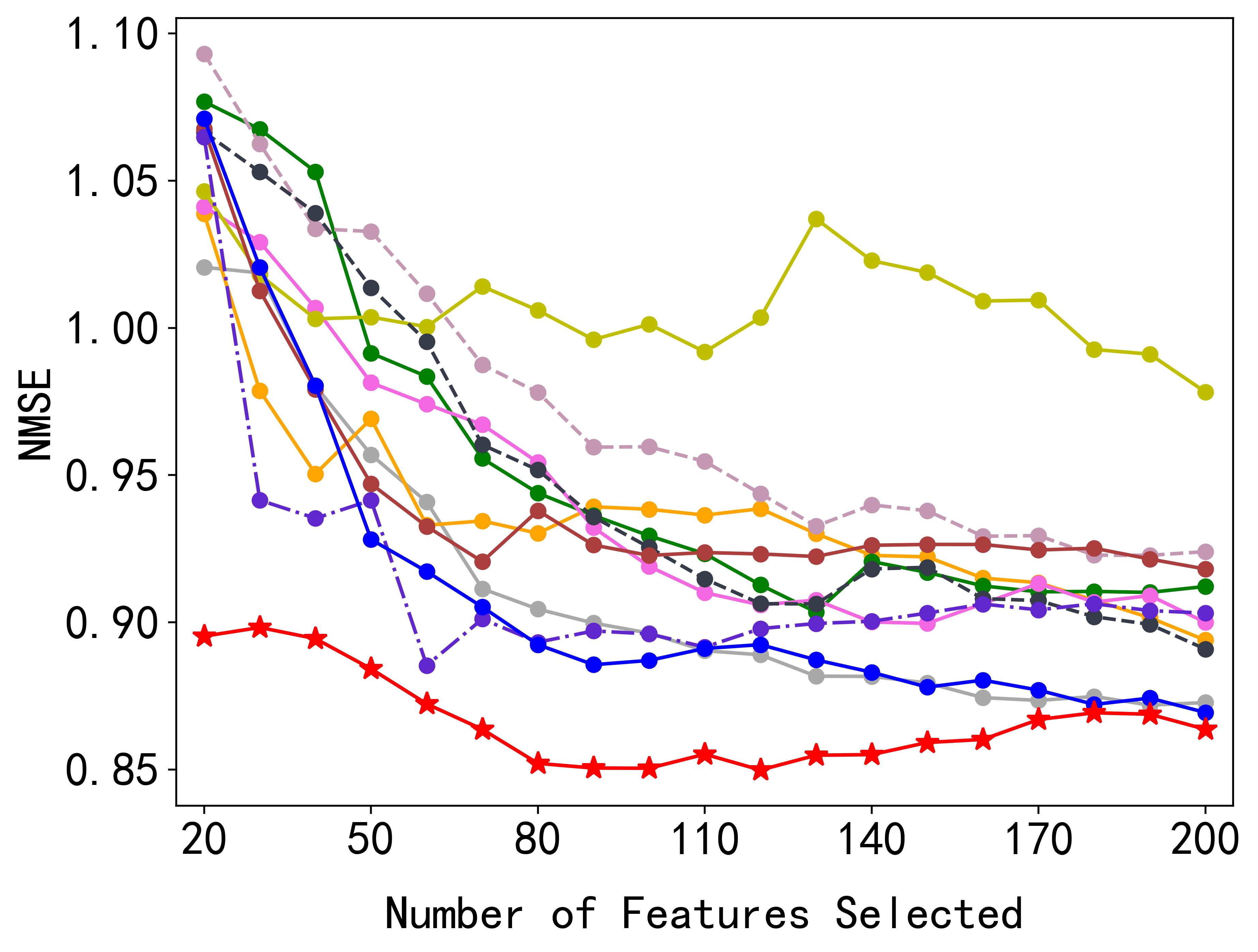
(c) Wheat599-env3

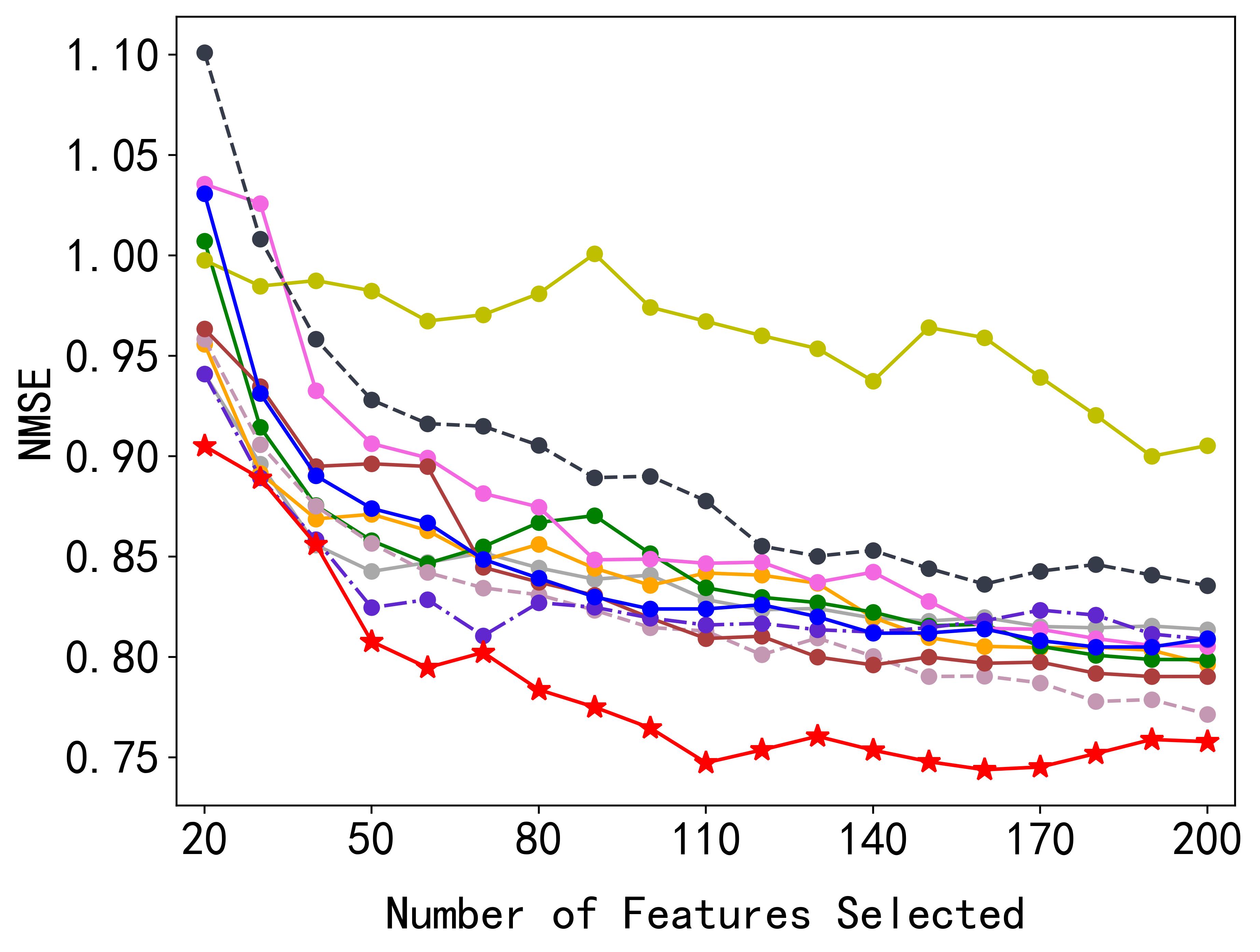
(d) Wheat599-env4

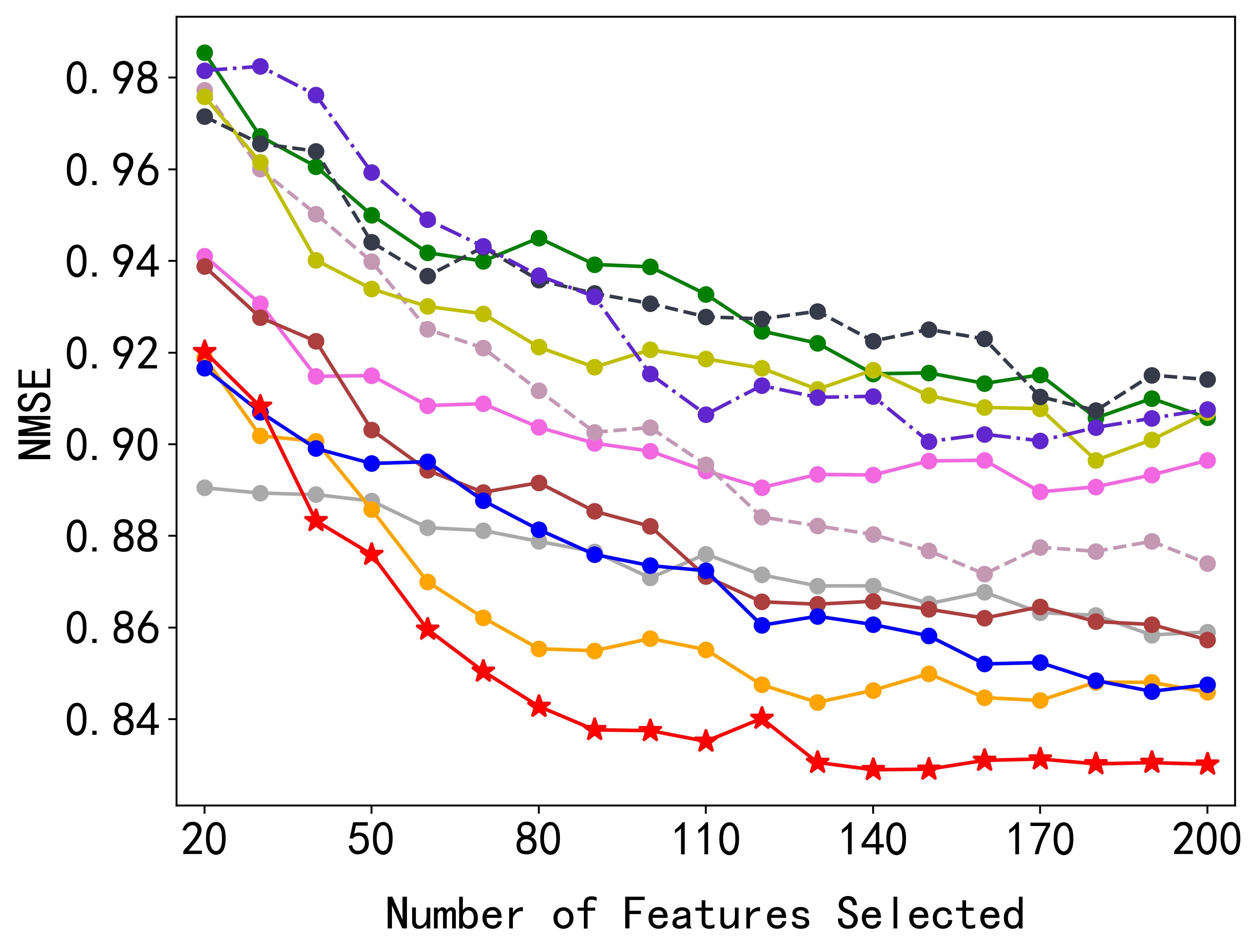
(e) SoyNAM-height

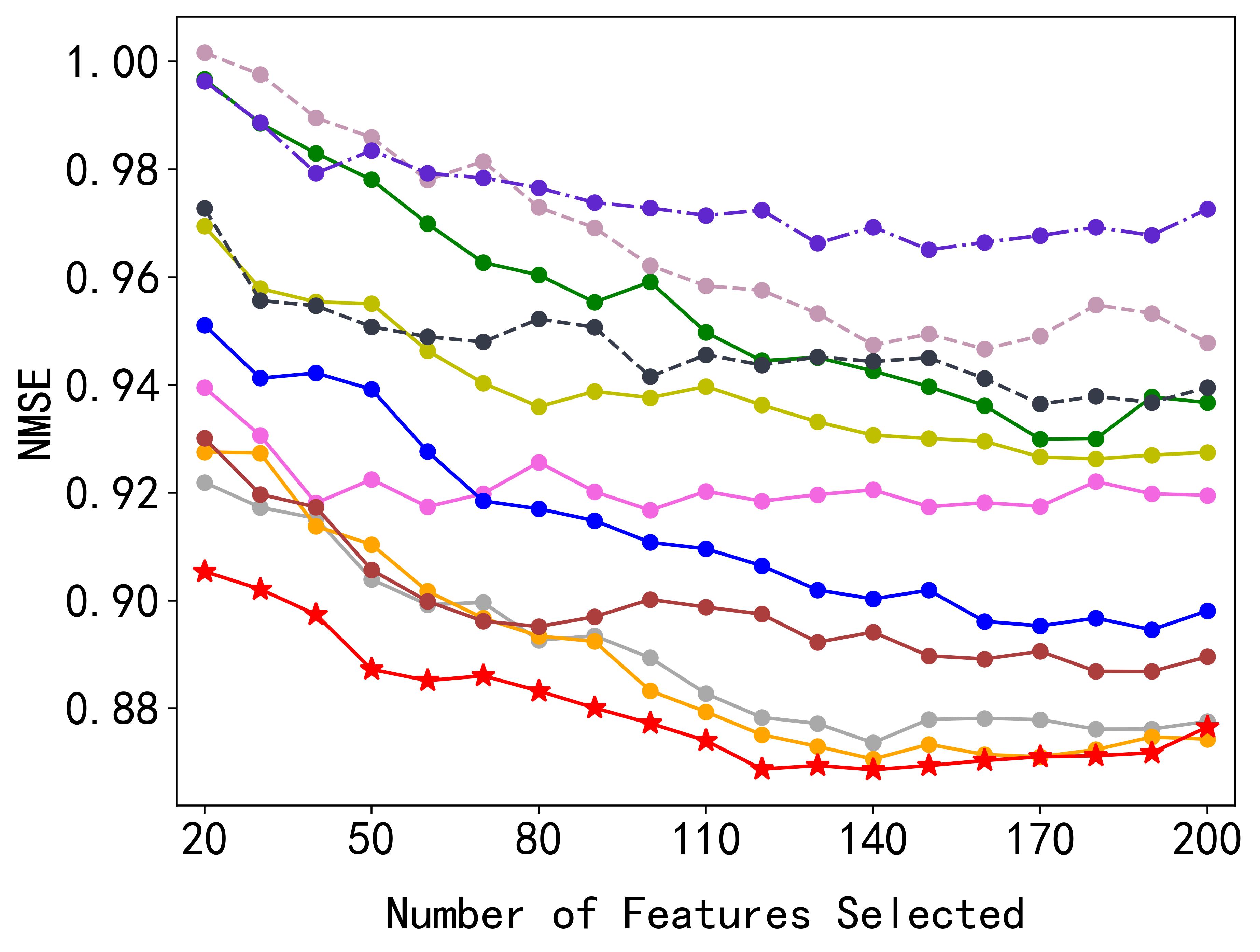
(f) SoyNAM-oil

(g) SoyNAM-moisture

(h) SoyNAM-protein

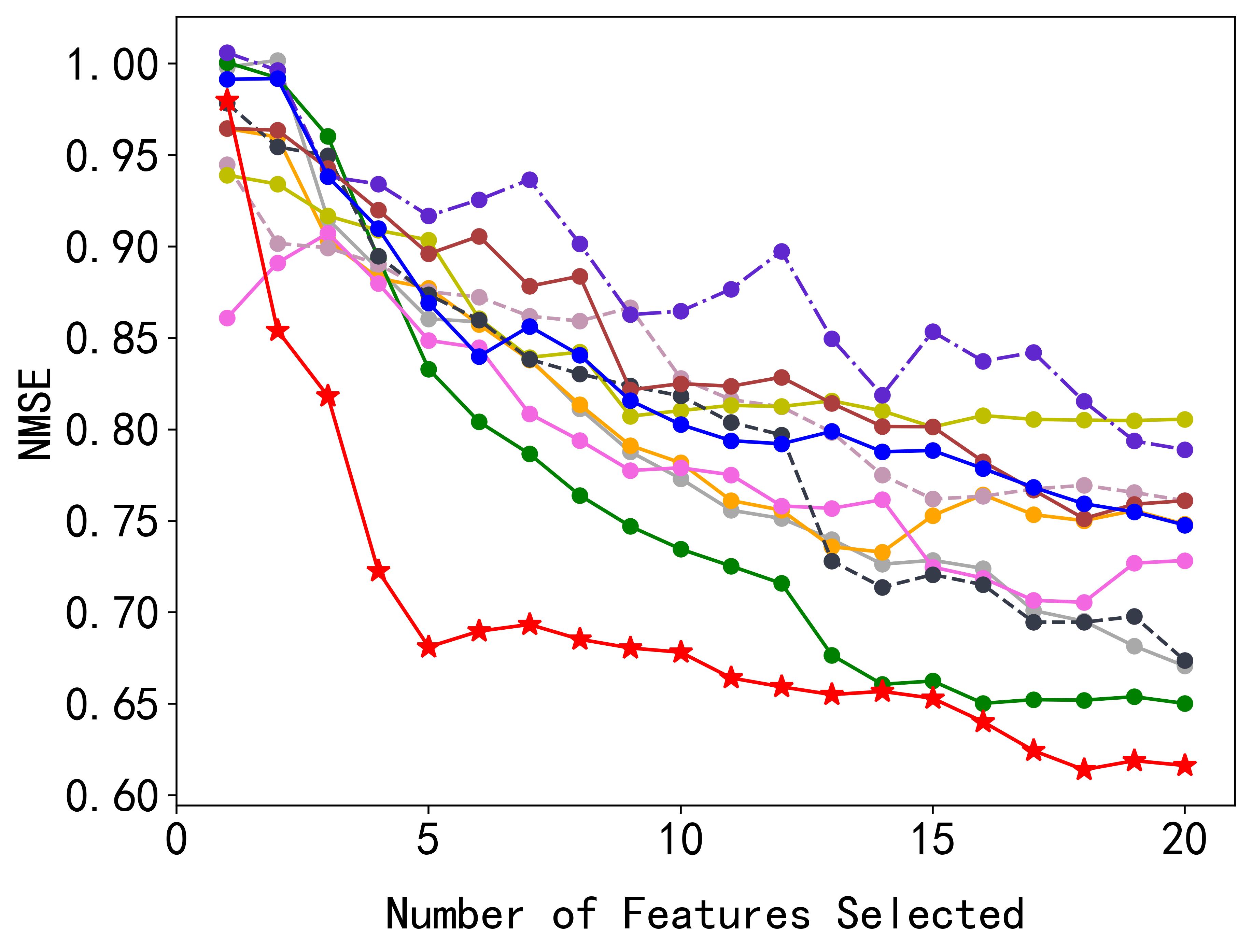
(i) CSD-1000R

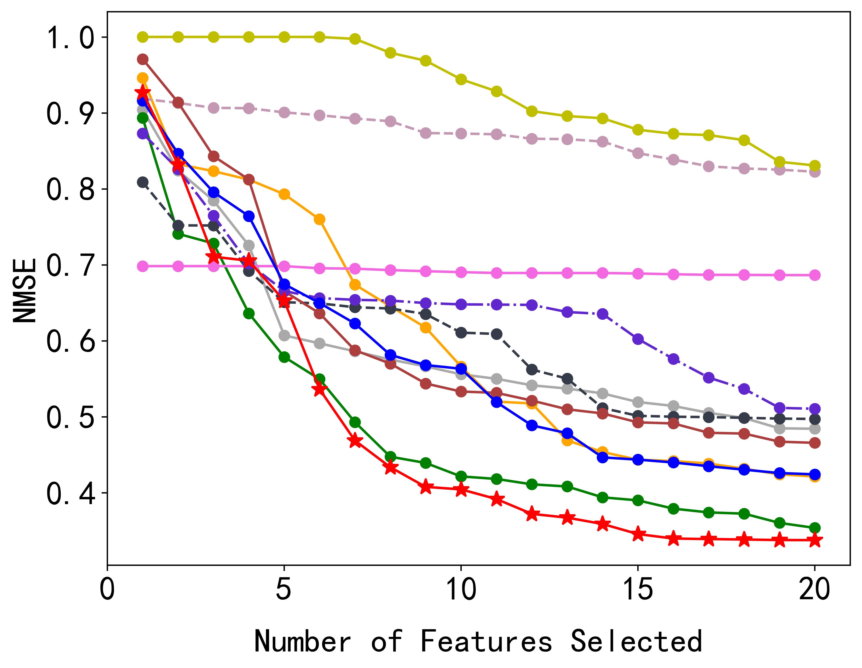
(j) SLICE

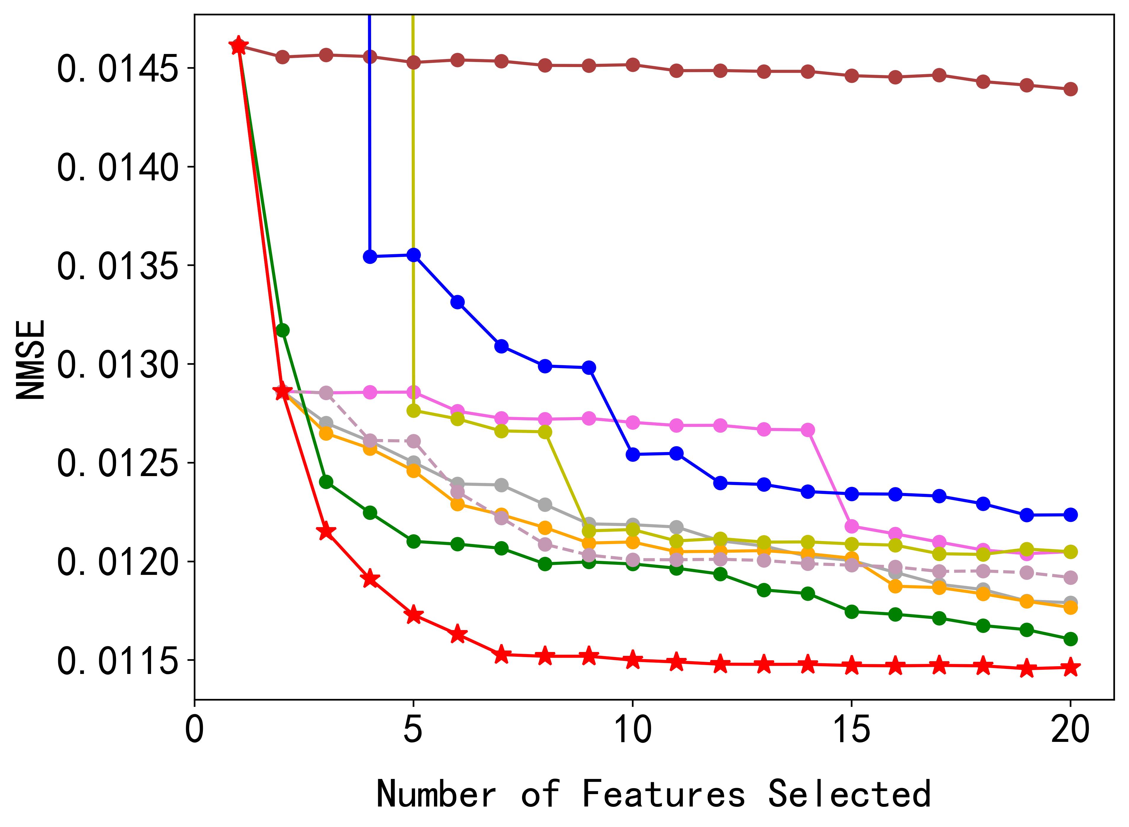
(k) COIL-2000

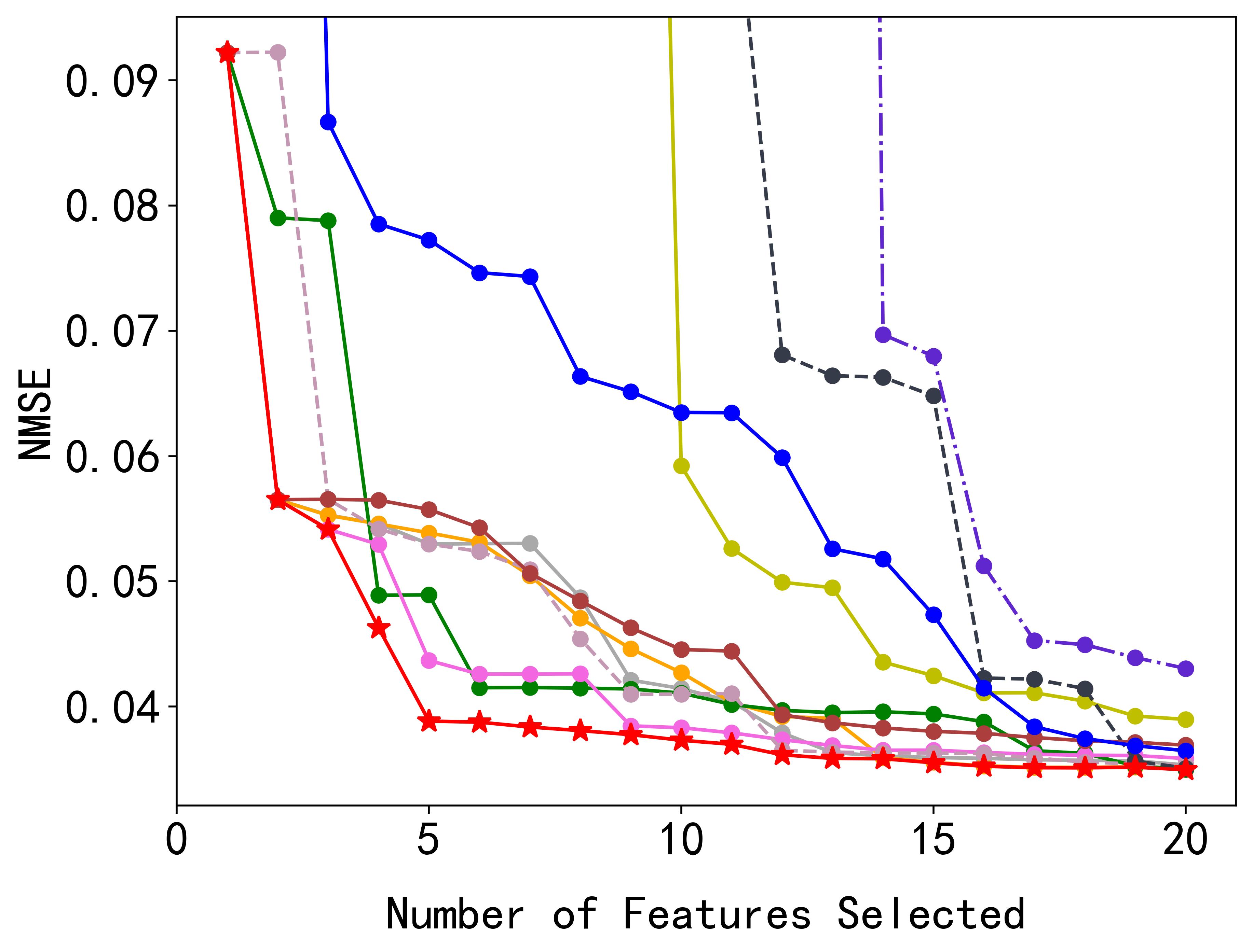
(l) SML

Figure 7: Regression dataset results

Appendix E Efficiency of Coding Redundancy

Comparison of CR and Mutual Information. When measuring the redundancy of features, we replace the traditional mutual information with our proposed coding redundancy (CR) to improve computational speed and provide natural support for continuous variables. To demonstrate the effectiveness of this replacement, we randomly selected 100 features from the ORL dataset and calculated the global redundancy of each feature using both CR and mutual information. We then appropriately normalized the results, as shown in Fig. 6. It can be observed that the global redundancy of features obtained using our method is nearly identical to the results from mutual information calculations. Moreover, in terms of computation time, our method is only 0.192% of the time required for mutual information, demonstrating that our proposed approach can replace mutual information to some extent when calculating global redundancy and provide a computational speedup.

Appendix F Regression and Classification Results

We depict comparison curves for all datasets in Fig. 7 and Fig. 8.

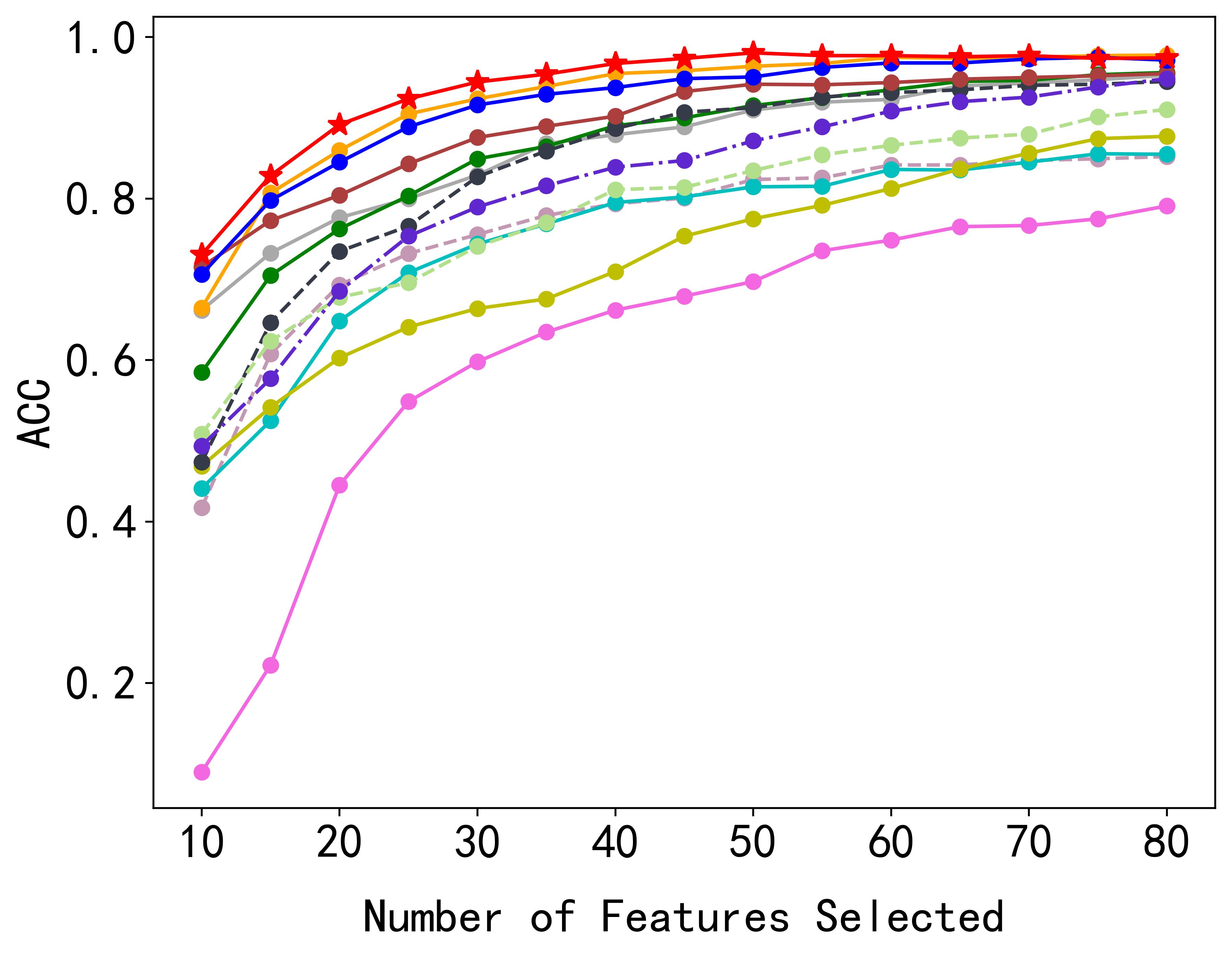
(a) COIL20

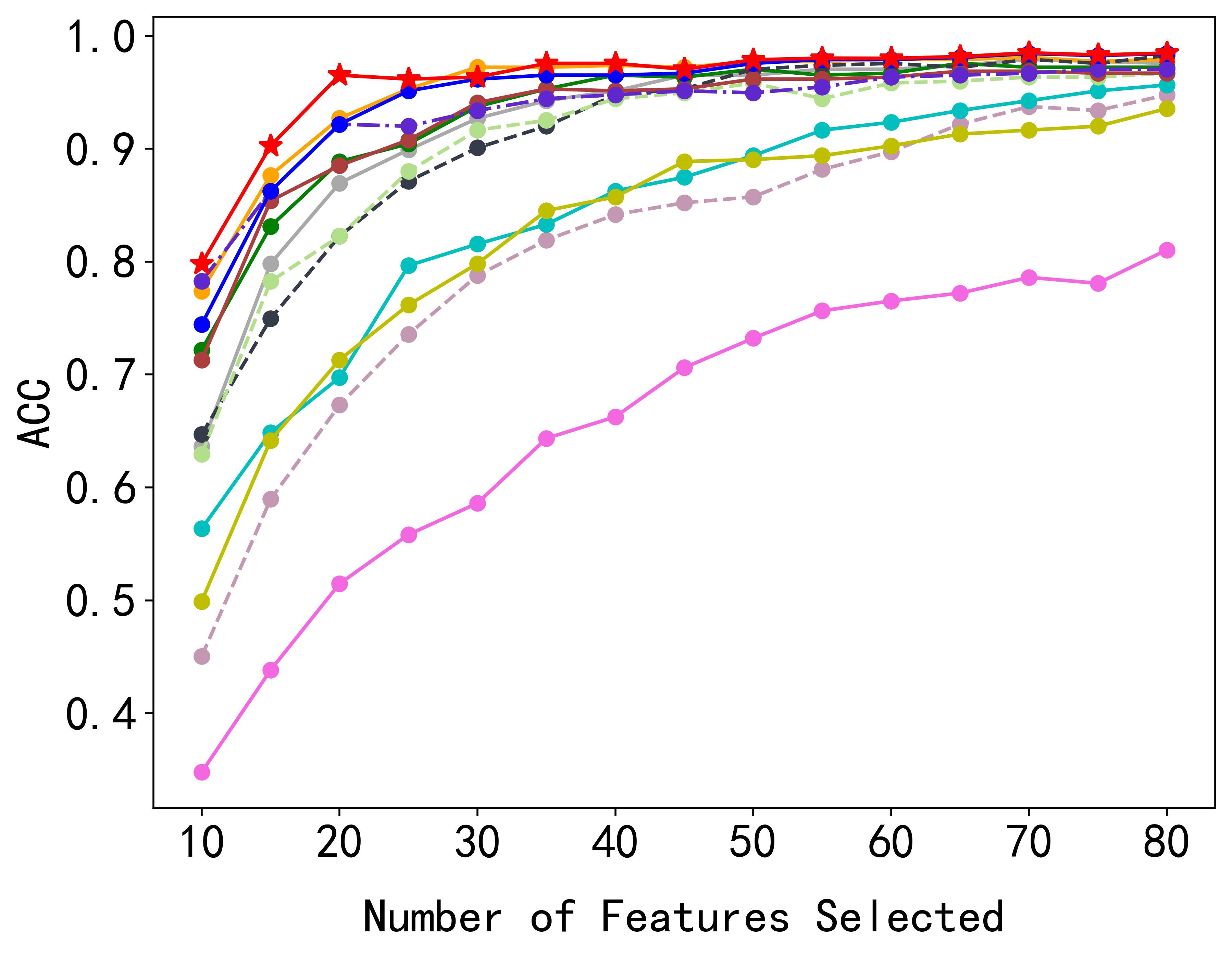
(b) UMIST

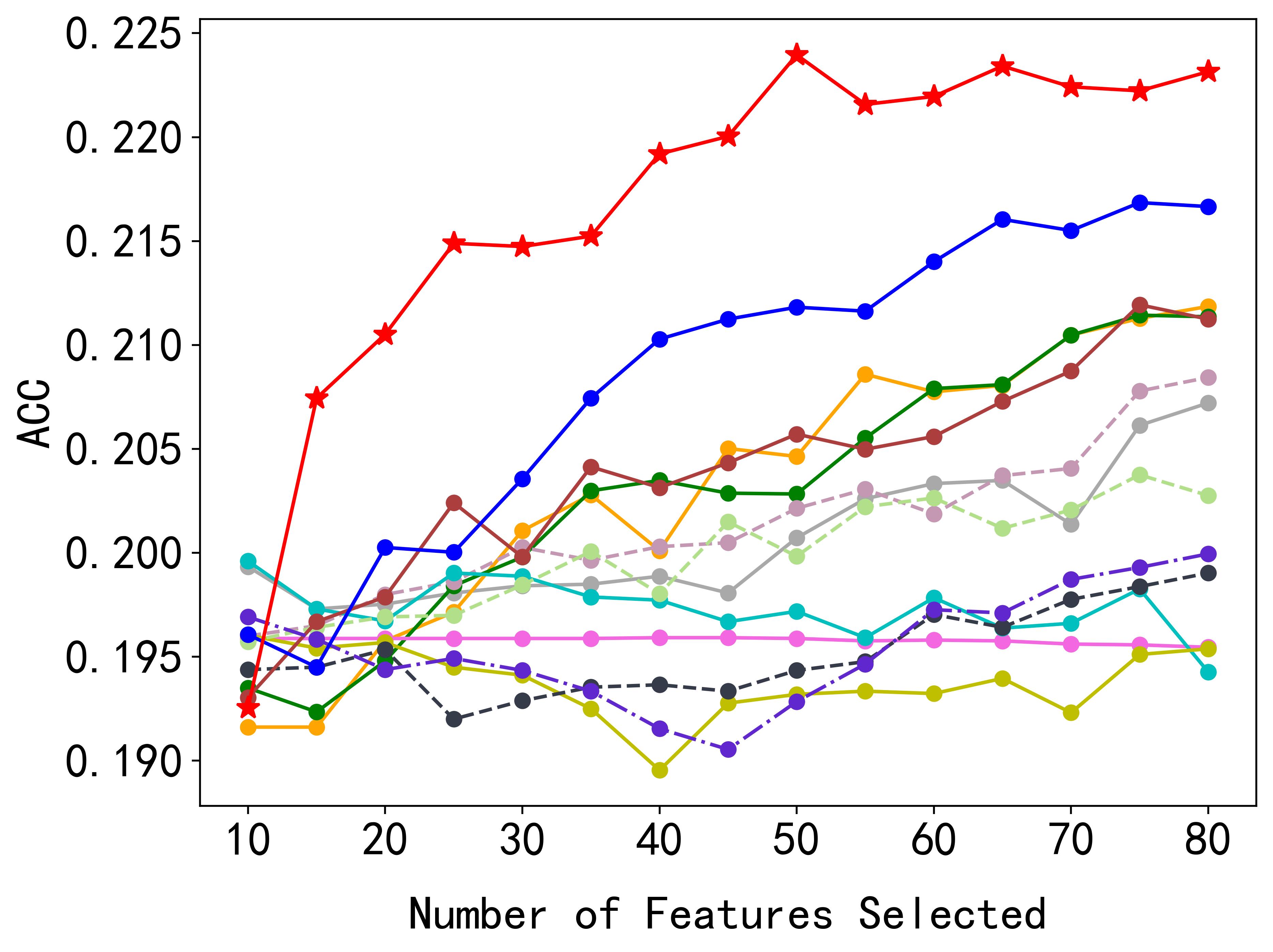
(c) SVHN

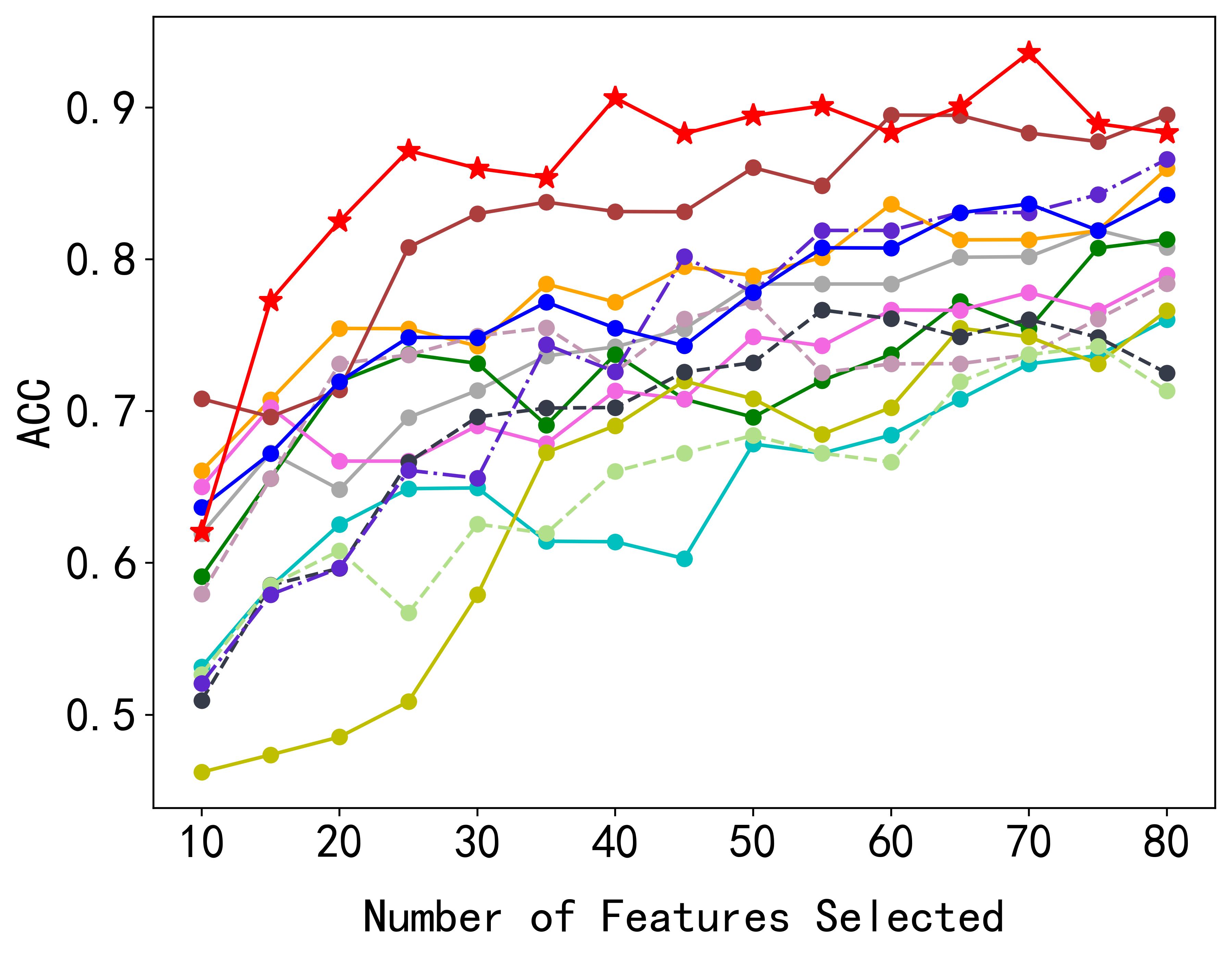
(d) TOX

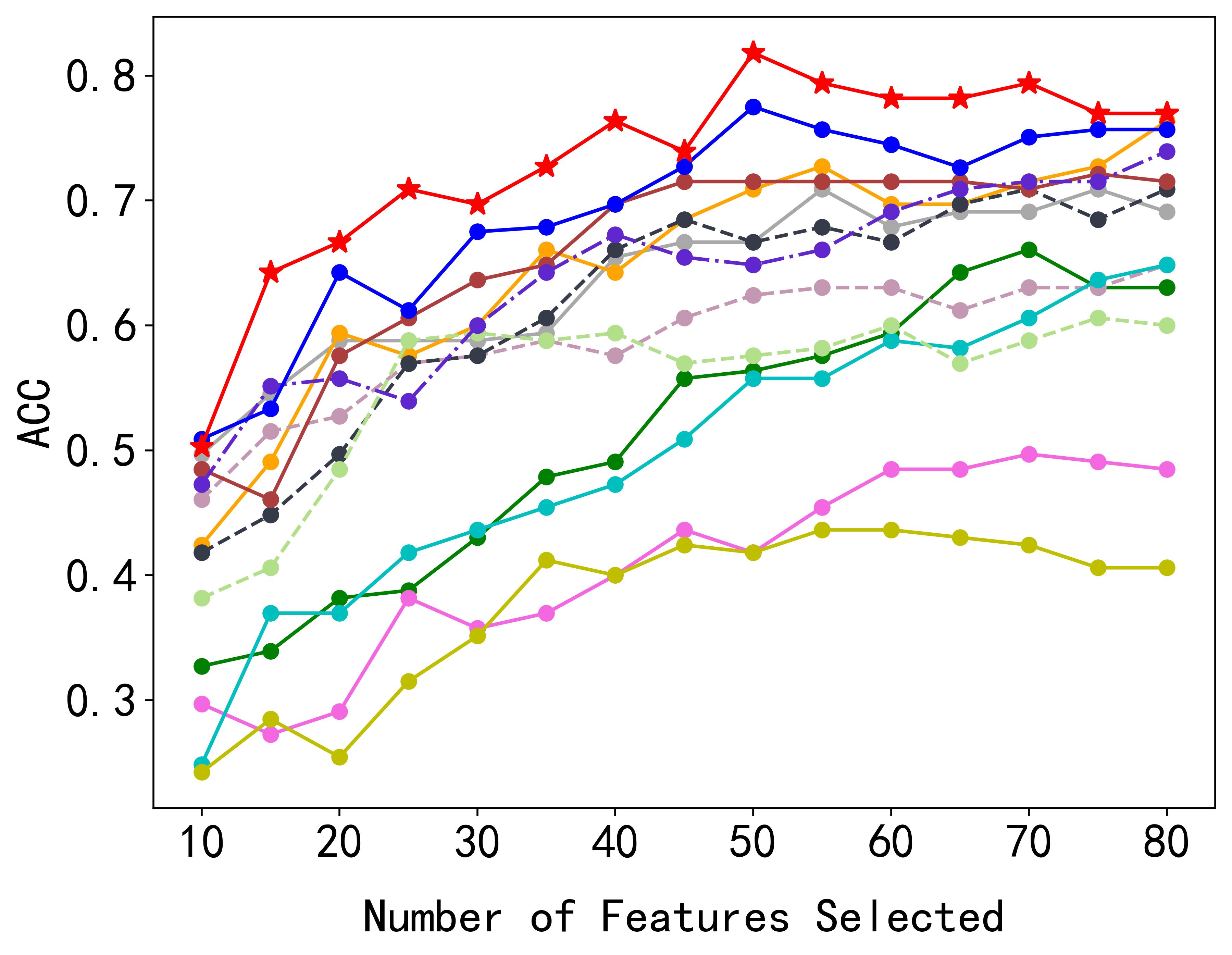
(e) YALE

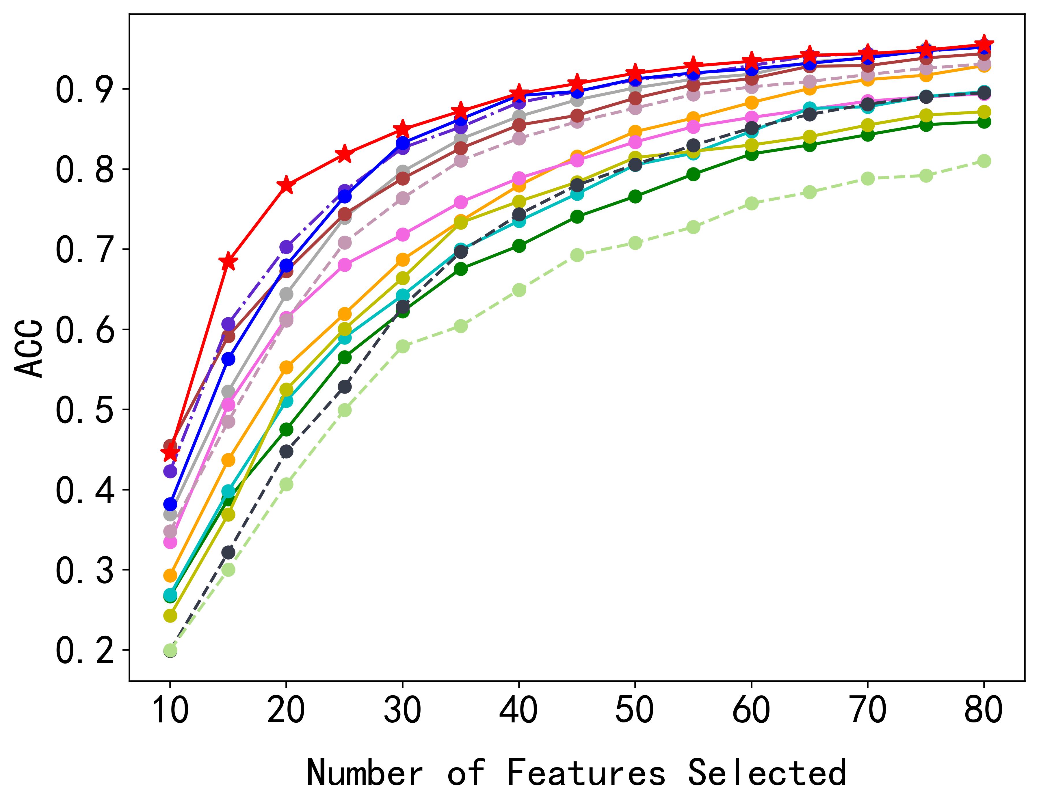
(f) YALEB

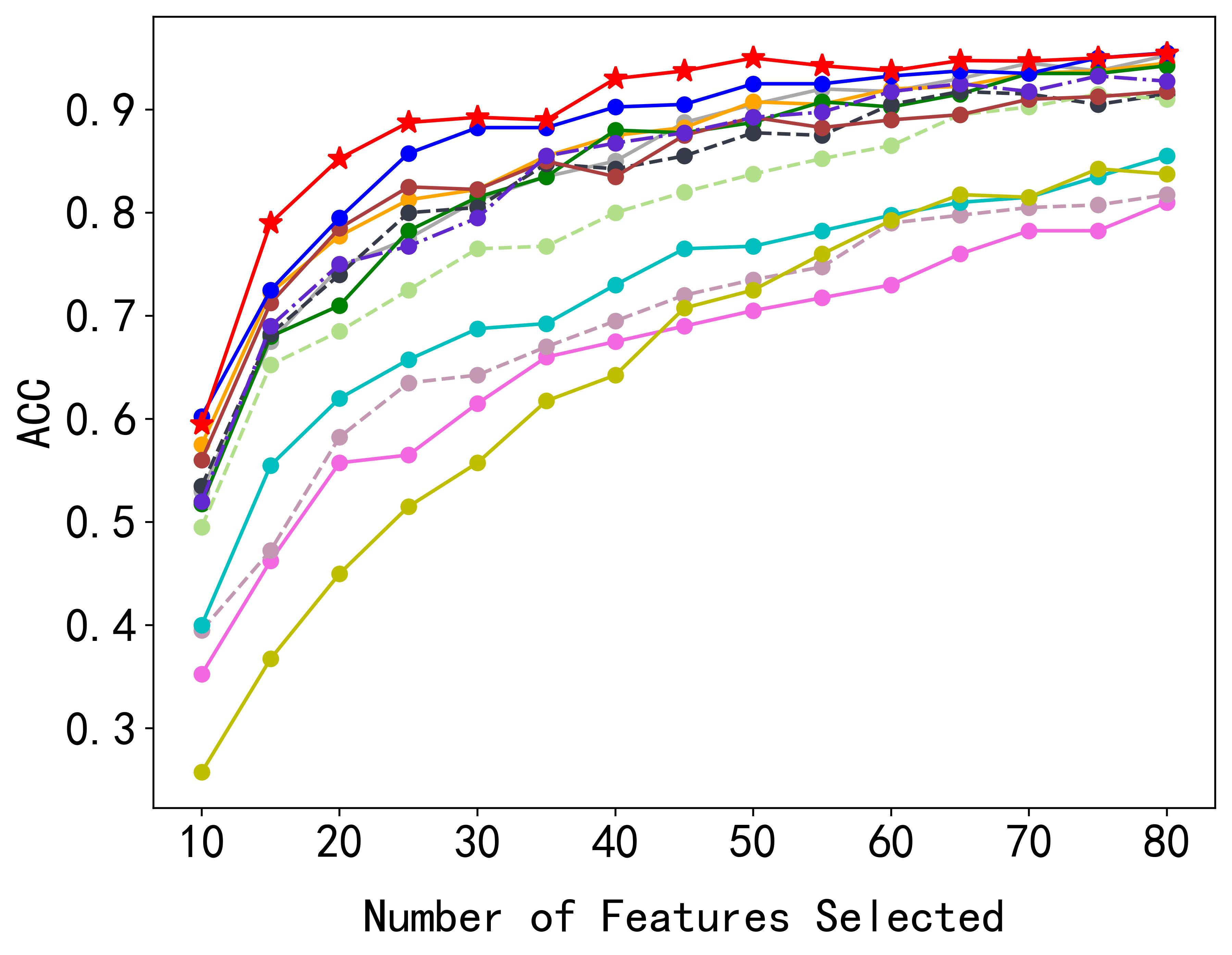
(g) ORL

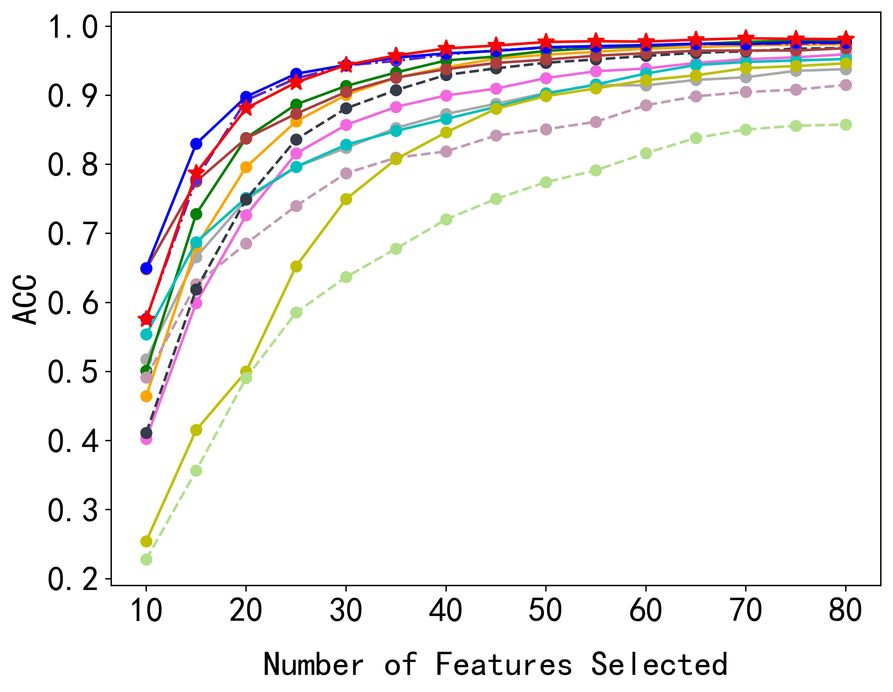
(h) PIE-05

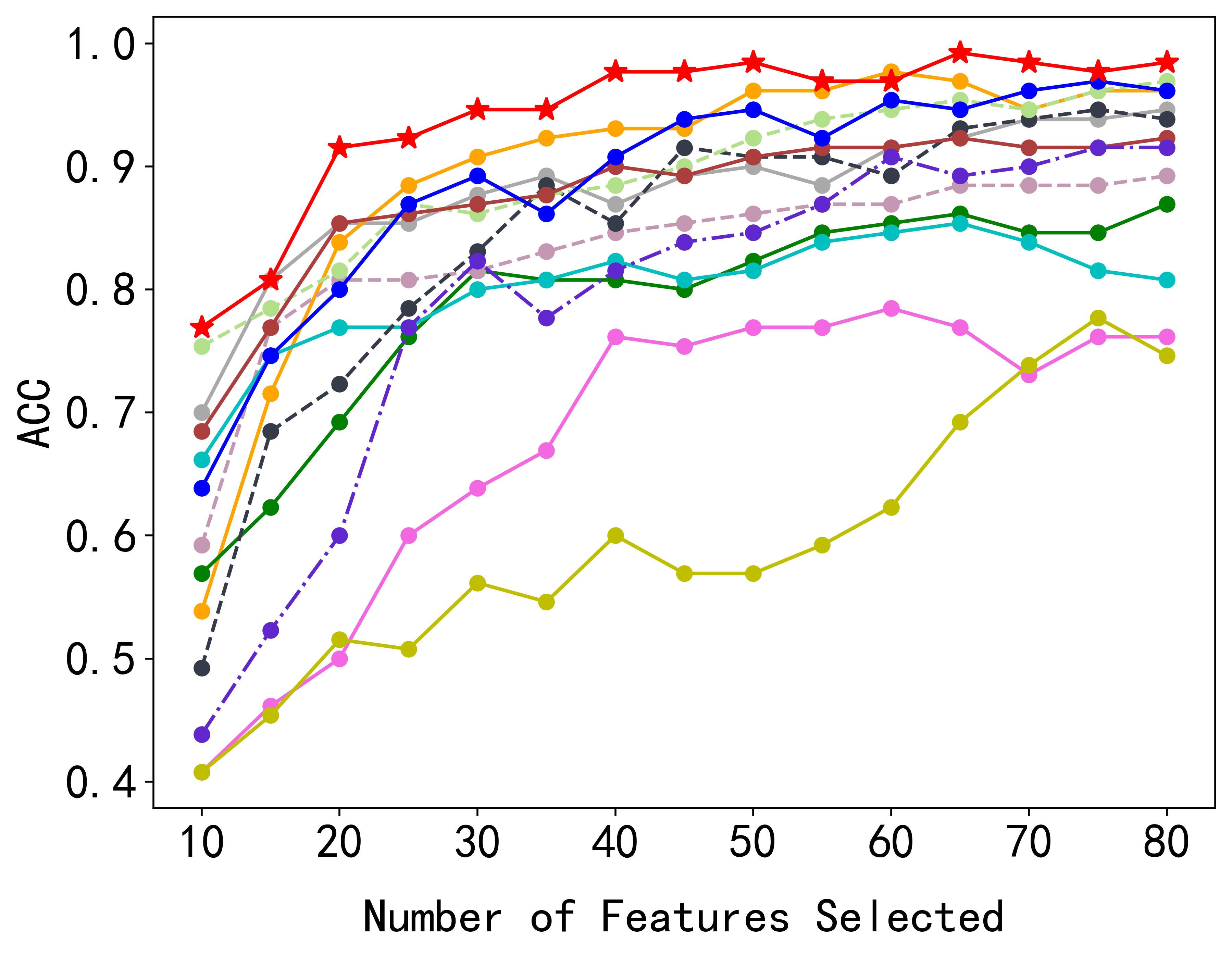
(i) warpAR10P

Figure 8: Classification dataset results

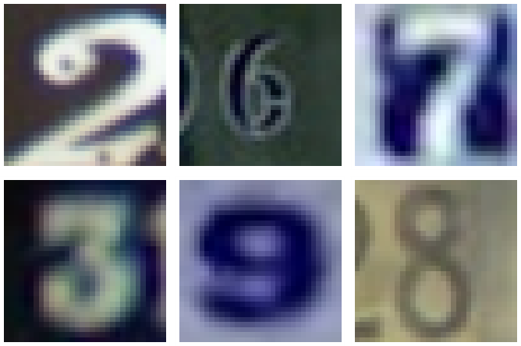
Figure 9: Example of the SVHN dataset

Appendix G Visualization Analysis

To further explore the differences in feature selection methods, we visualized the features selected by various methods in the SVHN dataset. Specifically, we ranked the features selected by each method, set the positions corresponding to the top 500 features to 255, set positions from 500 to 1500 to 127, and set the remaining positions to 0. Then, we merged the values of the three RGB channels to obtain the attention differences of the feature selection algorithms across the entire image. The results are shown in Fig. 10. It can be observed that our method focuses the most on the middle region of the image and gradually spreads to the edges, which aligns well with human observation patterns. In contrast, the STG algorithm and Relief algorithm are overly concentrated in the middle region of the image, which can result in poor performance when dealing with digits like 2 and 7 that occupy the top and bottom edges of the image, as shown in Fig. 9. XGB and Bf, on the other hand, have overly dispersed focus points and do not concentrate on the high-frequency areas where relevant information is likely to be found, potentially missing important information. PPMCC appears to focus too much on regions resembling noise, leading to increased attention to image edges.

Figure 10: Visualization of results

Appendix H Runtime Comparison

To further compare the differences in runtime among different algorithms, we selected the largest datasets for experiments in both regression and classification tasks. For the regression task, the SLICE dataset was used, while for the classification task, the SVHN dataset was chosen, with approximately the top 5% and top 2% of features selected, respectively. The experimental results are shown in Figure 11 and Figure 12. It can be observed that our time advantage becomes even more pronounced on large-scale datasets.

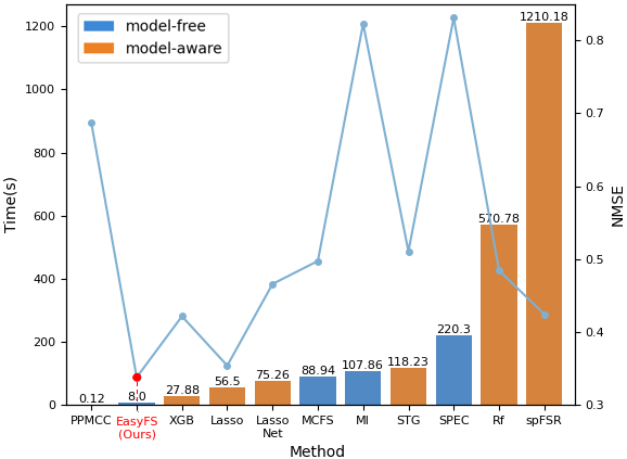
Figure 11: Runtime (by column) and NMSE (by curve) on the SLICE dataset

Figure 12: Runtime (by column) and Accuracy (by curve) on the SVHN dataset

References

- Akman et al. (2023) Akman, D. V., Malekipirbazari, M., Yenice, Z. D., Yeo, A., Adhikari, N., Wong, Y. K., Abbasi, B., and Gumus, A. T. k-best feature selection and ranking via stochastic approximation. Expert Systems with Applications, 213:118864, 2023.
- Bolón-Canedo et al. (2014) Bolón-Canedo, V., Sánchez-Marono, N., Alonso-Betanzos, A., Benítez, J. M., and Herrera, F. A review of microarray datasets and applied feature selection methods. Information sciences, 282:111–135, 2014.
- Cai et al. (2010) Cai, D., Zhang, C., and He, X. Unsupervised feature selection for multi-cluster data. In Proceedings of the 16th ACM SIGKDD international conference on Knowledge discovery and data mining, pp. 333–342, 2010.
- Chen et al. (2013) Chen, B., Chen, L., and Chen, Y. Efficient ant colony optimization for image feature selection. Signal processing, 93(6):1566–1576, 2013.
- Chen et al. (2017) Chen, J., Stern, M., Wainwright, M. J., and Jordan, M. I. Kernel feature selection via conditional covariance minimization. Advances in Neural Information Processing Systems, 30, 2017.
- Chen & Guestrin (2016) Chen, T. and Guestrin, C. Xgboost: A scalable tree boosting system. In Proceedings of the 22nd acm sigkdd international conference on knowledge discovery and data mining, pp. 785–794, 2016.
- Cohen et al. (2023) Cohen, D., Shnitzer, T., Kluger, Y., and Talmon, R. Few-sample feature selection via feature manifold learning. In International Conference on Machine Learning, pp. 6296–6319. PMLR, 2023.
- Díaz-Uriarte & Alvarez de Andrés (2006) Díaz-Uriarte, R. and Alvarez de Andrés, S. Gene selection and classification of microarray data using random forest. BMC bioinformatics, 7:1–13, 2006.
- Estévez et al. (2009) Estévez, P. A., Tesmer, M., Perez, C. A., and Zurada, J. M. Normalized mutual information feature selection. IEEE Transactions on neural networks, 20(2):189–201, 2009.
- Frank (2010) Frank, A. Uci machine learning repository. http://archive. ics. uci. edu/ml, 2010.
- Gan & Zhang (2021) Gan, M. and Zhang, L. Iteratively local fisher score for feature selection. Applied Intelligence, 51:6167–6181, 2021.
- Georghiades et al. (2001) Georghiades, A. S., Belhumeur, P. N., and Kriegman, D. J. From few to many: Illumination cone models for face recognition under variable lighting and pose. IEEE transactions on pattern analysis and machine intelligence, 23(6):643–660, 2001.
- Graham & Allinson (1998) Graham, D. B. and Allinson, N. M. Characterising virtual eigensignatures for general purpose face recognition. In Face recognition: from theory to applications, pp. 446–456. Springer, 1998.
- Gu et al. (2012) Gu, Q., Li, Z., and Han, J. Generalized fisher score for feature selection. arXiv preprint arXiv:1202.3725, 2012.
- Hall (1999) Hall, M. A. Correlation-based feature selection for machine learning. PhD thesis, The University of Waikato, 1999.
- Han et al. (2018) Han, K., Wang, Y., Zhang, C., Li, C., and Xu, C. Autoencoder inspired unsupervised feature selection. In 2018 IEEE international conference on acoustics, speech and signal processing (ICASSP), pp. 2941–2945. IEEE, 2018.
- Hancer et al. (2018) Hancer, E., Xue, B., and Zhang, M. Differential evolution for filter feature selection based on information theory and feature ranking. Knowledge-Based Systems, 140:103–119, 2018.
- He et al. (2016) He, K., Zhang, X., Ren, S., and Sun, J. Deep residual learning for image recognition. In Proceedings of the IEEE conference on computer vision and pattern recognition, pp. 770–778, 2016.
- He et al. (2005) He, X., Cai, D., and Niyogi, P. Laplacian score for feature selection. In Weiss, Y., Schölkopf, B., and Platt, J. (eds.), Advances in Neural Information Processing Systems, volume 18. MIT Press, 2005. URL https://proceedings.neurips.cc/paper_files/paper/2005/file/b5b03f06271f8917685d14cea7c6c50a-Paper.pdf.
- Imrie et al. (2022) Imrie, F., Norcliffe, A., Liò, P., and van der Schaar, M. Composite feature selection using deep ensembles. Advances in Neural Information Processing Systems, 35:36142–36160, 2022.
- Jaeger (2002) Jaeger, H. Adaptive nonlinear system identification with echo state networks. Advances in neural information processing systems, 15, 2002.
- Jia et al. (2022) Jia, W., Sun, M., Lian, J., and Hou, S. Feature dimensionality reduction: a review. Complex & Intelligent Systems, 8(3):2663–2693, 2022.
- Khalajzadeh et al. (2014) Khalajzadeh, H., Mansouri, M., and Teshnehlab, M. Face recognition using convolutional neural network and simple logistic classifier. In Soft Computing in Industrial Applications: Proceedings of the 17th Online World Conference on Soft Computing in Industrial Applications, pp. 197–207. Springer, 2014.
- Lemhadri et al. (2021) Lemhadri, I., Ruan, F., and Tibshirani, R. Lassonet: Neural networks with feature sparsity. In International conference on artificial intelligence and statistics, pp. 10–18. PMLR, 2021.
- Li et al. (2017) Li, J., Cheng, K., Wang, S., Morstatter, F., Trevino, R. P., Tang, J., and Liu, H. Feature selection: A data perspective. ACM computing surveys (CSUR), 50(6):1–45, 2017.
- Li et al. (2016) Li, Y., Chen, C.-Y., and Wasserman, W. W. Deep feature selection: theory and application to identify enhancers and promoters. Journal of Computational Biology, 23(5):322–336, 2016.
- Lin & Tang (2006) Lin, D. and Tang, X. Conditional infomax learning: An integrated framework for feature extraction and fusion. Lecture Notes in Computer Science,Lecture Notes in Computer Science, Jan 2006.
- Liu et al. (2019) Liu, Y., Wang, D., He, F., Wang, J., Joshi, T., and Xu, D. Phenotype prediction and genome-wide association study using deep convolutional neural network of soybean. Frontiers in genetics, 10:1091, 2019.
- McLaren et al. (2005) McLaren, C. G., Bruskiewich, R. M., Portugal, A. M., and Cosico, A. B. The international rice information system. a platform for meta-analysis of rice crop data. Plant Physiology, 139(2):637–642, 2005.
- Meyer & Bontempi (2006) Meyer, P. E. and Bontempi, G. On the Use of Variable Complementarity for Feature Selection in Cancer Classification, pp. 91–102. Jan 2006. doi: 10.1007/11732242˙9. URL http://dx.doi.org/10.1007/11732242_9.
- Mirzaei et al. (2020) Mirzaei, A., Pourahmadi, V., Soltani, M., and Sheikhzadeh, H. Deep feature selection using a teacher-student network. Neurocomputing, 383:396–408, 2020.
- Moradipari et al. (2022) Moradipari, A., Turan, B., Abbasi-Yadkori, Y., Alizadeh, M., and Ghavamzadeh, M. Feature and parameter selection in stochastic linear bandits. In International Conference on Machine Learning, pp. 15927–15958. PMLR, 2022.
- Musil et al. (2019) Musil, F., Willatt, M. J., Langovoy, M. A., and Ceriotti, M. Fast and accurate uncertainty estimation in chemical machine learning. Journal of chemical theory and computation, 15(2):906–915, 2019.
- Muthukrishnan & Rohini (2016) Muthukrishnan, R. and Rohini, R. Lasso: A feature selection technique in predictive modeling for machine learning. In 2016 IEEE international conference on advances in computer applications (ICACA), pp. 18–20. IEEE, 2016.
- Nene et al. (1996) Nene, S. A., Nayar, S. K., Murase, H., et al. Columbia object image library (coil-20). 1996.
- Netzer et al. (2011) Netzer, Y., Wang, T., Coates, A., Bissacco, A., Wu, B., and Ng, A. Y. Reading digits in natural images with unsupervised feature learning. 2011.
- Pedregosa et al. (2011) Pedregosa, F., Varoquaux, G., Gramfort, A., Michel, V., Thirion, B., Grisel, O., Blondel, M., Prettenhofer, P., Weiss, R., Dubourg, V., et al. Scikit-learn: Machine learning in python. the Journal of machine Learning research, 12:2825–2830, 2011.
- Peng et al. (2005) Peng, H., Long, F., and Ding, C. Feature selection based on mutual information criteria of max-dependency, max-relevance, and min-redundancy. IEEE Transactions on pattern analysis and machine intelligence, 27(8):1226–1238, 2005.
- Robnik-Šikonja & Kononenko (2003a) Robnik-Šikonja, M. and Kononenko, I. Theoretical and empirical analysis of relieff and rrelieff. Machine learning, 53:23–69, 2003a.
- Robnik-Šikonja & Kononenko (2003b) Robnik-Šikonja, M. and Kononenko, I. Theoretical and empirical analysis of relieff and rrelieff. Machine learning, 53:23–69, 2003b.
- Roffo et al. (2020) Roffo, G., Melzi, S., Castellani, U., Vinciarelli, A., and Cristani, M. Infinite feature selection: a graph-based feature filtering approach. IEEE Transactions on Pattern Analysis and Machine Intelligence, 43(12):4396–4410, 2020.
- Ross (2014) Ross, B. C. Mutual information between discrete and continuous data sets. PloS one, 9(2):e87357, 2014.
- Rustam et al. (2019) Rustam, Z., Kintandani, P., et al. Application of support vector regression in indonesian stock price prediction with feature selection using particle swarm optimisation. Modelling and Simulation in Engineering, 2019, 2019.
- Samaria & Harter (1994) Samaria, F. S. and Harter, A. C. Parameterisation of a stochastic model for human face identification. In Proceedings of 1994 IEEE workshop on applications of computer vision, pp. 138–142. IEEE, 1994.
- Sim et al. (2002) Sim, T., Baker, S., and Bsat, M. The cmu pose, illumination, and expression (pie) database. In Proceedings of fifth IEEE international conference on automatic face gesture recognition, pp. 53–58. IEEE, 2002.
- Tibshirani (1996) Tibshirani, R. Regression shrinkage and selection via the lasso. Journal of the Royal Statistical Society Series B: Statistical Methodology, 58(1):267–288, 1996.
- Wang et al. (2023) Wang, K., Abid, M. A., Rasheed, A., Crossa, J., Hearne, S., and Li, H. Dnngp, a deep neural network-based method for genomic prediction using multi-omics data in plants. Molecular Plant, 16(1):279–293, 2023.
- Wojtas & Chen (2020) Wojtas, M. and Chen, K. Feature importance ranking for deep learning. Advances in Neural Information Processing Systems, 33:5105–5114, 2020.
- Xu et al. (2023) Xu, L., Wang, R., Nie, F., and Li, X. Efficient top-k feature selection using coordinate descent method. In Proceedings of the AAAI Conference on Artificial Intelligence, volume 37, pp. 10594–10601, 2023.
- Xue et al. (2018) Xue, X., Yao, M., and Wu, Z. A novel ensemble-based wrapper method for feature selection using extreme learning machine and genetic algorithm. Knowledge and Information Systems, 57:389–412, 2018.
- Yamada et al. (2020) Yamada, Y., Lindenbaum, O., Negahban, S., and Kluger, Y. Feature selection using stochastic gates. In International Conference on Machine Learning, pp. 10648–10659. PMLR, 2020.
- Yin et al. (2014) Yin, S., Ding, S. X., Xie, X., and Luo, H. A review on basic data-driven approaches for industrial process monitoring. IEEE Transactions on Industrial electronics, 61(11):6418–6428, 2014.
- Yu et al. (2020) Yu, Y., Chan, K. H. R., You, C., Song, C., and Ma, Y. Learning diverse and discriminative representations via the principle of maximal coding rate reduction. Advances in Neural Information Processing Systems, 33:9422–9434, 2020.
- Zebari et al. (2020) Zebari, R., Abdulazeez, A., Zeebaree, D., Zebari, D., and Saeed, J. A comprehensive review of dimensionality reduction techniques for feature selection and feature extraction. Journal of Applied Science and Technology Trends, 1(2):56–70, 2020.
- Zhao & Liu (2007) Zhao, Z. and Liu, H. Spectral feature selection for supervised and unsupervised learning. In Proceedings of the 24th international conference on Machine learning, pp. 1151–1157, 2007.