YOLO-CIANNA: Galaxy detection with deep learning in radio data

Abstract

Context. The upcoming Square Kilometer Array (SKA) will set a new standard regarding data volume generated by an astronomical instrument, which is likely to challenge widely adopted data analysis tools that scale inadequately with the data size.

Aims. This study aims to develop a new source detection and characterization method for massive radio astronomical datasets by adapting modern deep-learning object detection techniques. These approaches have proved their efficiency on complex computer vision tasks, and we seek to identify their specific strengths and weaknesses when applied to astronomical data.

Methods. We introduce YOLO-CIANNA, a highly customized deep-learning object detector designed specifically for astronomical datasets. This paper presents the method and describes all the low-level adaptations required to address the specific challenges of radio-astronomical images. We demonstrate this method’s capabilities using simulated 2D continuum images from the SKA Observatory (SKAO) Science Data Challenge 1 (SDC1) dataset.

Results. Our method outperforms every other published result on the specific SDC1 dataset. Using the SDC1 metric, we improve the challenge-winning score by +139% and the score of the only other post-challenge participation by +61%. Our catalog has a detection purity of 94% while detecting 40 to 60 % more sources than previous top-score results with a total of almost 680000 properly detected sources. The trained model can also be forced to reach 99% purity in post-process and still detect 10 to 30% more sources than the other top-score methods. Our method is efficient at low signal-to-noise ratio and exhibits strong characterization accuracy. It is also capable of real-time detection, with a peak prediction speed of 500 images of $512{\times}512$ pixels per second on a single GPU.

Conclusions. YOLO-CIANNA achieves state-of-the-art detection and characterization results on the simulated SDC1 dataset. This is encouraging regarding its potential capability over observational data from SKA precursors. The method is open source and included in the wider CIANNA framework. We provide scripts to train and apply this method to the SDC1 dataset in the CIANNA repository.

1 Introduction

Modern astronomical instruments generate ever-increasing data volumes, following the need for better resolution, sensitivity, and larger wavelength coverage. Astronomical datasets are often highly dimensional and require precise encoding of the measurements due to a high dynamic range. In addition, it is often necessary to preserve the raw data due to iterative improvement of the analysis pipelines. Radio-astronomy is strongly affected by the explosion of data volumes, especially regarding giant radio interferometers. In particular, the upcoming Square Kilometer Array (SKA, Braun et al., 2019) is expected to have an unprecedented real-time data rate and to produce a remarkable amount of stored science data products with around 700 PB of archived data per year. This instrument is foreseen to have the necessary sensitivity to set constraints on the cosmic dawn and the epoch of reionization and to trace the evolution of astronomical objects over cosmological times. With such volume and complexity of data, some classical analysis methods and tools employed in radio astronomy for decades start to exhibit scaling limits.

In this context, the SKA Observatory (SKAO) started the organization of recurrent Science Data Challenges (SDCs) to gather astronomers from the international community around simulated datasets that resemble future SKA data products. The objective is to evaluate the suitability of existing analysis methods and encourage the development of new ones. It is also an opportunity for astronomers to get familiar with the nature of such datasets and to gain experience in their exploration.

The first edition, SDC1 (Bonaldi et al., 2021), focused on a source detection and characterization task over simulated continuum radio images at different frequencies and integration times. We show a cutout from one of the SDC1 images in Fig. 1, illustrating the source density and the high dynamical range. Source-finding is a common task in astronomy and is often the first analysis to be done on a newly acquired image product. It is already performed by a variety of classical methods, for example, SExtractor (Bertin & Arnouts, 1996), SFIND (Hopkins et al., 2002), CUTEX (Molinari et al., 2011), BLOBCAT (Hales et al., 2012), AEGEAN (Hancock et al., 2018), DUCHAMP (Whiting, 2012), PyBDSF (Mohan & Rafferty, 2015), PROFOUND (Robotham et al., 2018). The obtained source catalogs can then be augmented with characterization information and used as primary data for subsequent analyses. This task is strongly affected by the increase in volume and dimensionality, making it a good proxy to evaluate the upcoming data handling challenges.

In the past decade, we observed an explosion in the machine learning (ML) methods usage in all fields, including astronomy and astrophysics (Huertas-Company & Lanusse, 2023). One of the advantages of ML methods is their good performance and efficiency scaling with data size and dimensionality. There is a considerable variety of ML approaches, so we only focus here on methods based on the deep artificial neural networks formalism (LeCun et al., 2015). Deep learning approaches have been extensively used for computer vision tasks, including the leading object detection application (Russakovsky et al., 2015; Everingham et al., 2010; Lin et al., 2014). While detection models have been extensively used in other domains for several years, they are not yet widely adopted in the astronomical community.

Deep learning object detection methods are usually separated into three families (Zhao et al., 2018). The first one represents segmentation models. Their main advantage is identifying which pixels belong to a given object type (semantic segmentation). Their main drawback is their symmetric structure (encoder and decoder) and the amount of work to be done near the image resolution, making them compute-intensive. They can also be used as a convenient structure for denoising tasks. This family is mainly represented by the U-Net (Ronneberger et al., 2015) method. Due to their proximity with classical source detection approaches, they have been employed for a variety of astronomical applications (e.g., Akeret et al., 2017; Vafaei Sadr et al., 2019; Lukic et al., 2019; Paillassa et al., 2020; Bianco et al., 2021; Makinen et al., 2021; Sortino et al., 2023; Håkansson et al., 2023).

The second family corresponds to the region-based detectors. They are often based on multi-stage neural networks that split the detection task into a region proposal step and a detection refinement step. They are the most employed for mission-critical tasks due to their accuracy. While faster than segmentation methods, the high detection accuracy models are compute-intensive due to the multi-stage process. This family is mainly represented by the R-CNN method (Girshick et al., 2013) and all its derivatives (e.g., Fast R-CNN, Faster R-CNN). Examples of astronomical applications with these methods are more limited, but it is increasing (e.g., Wu et al., 2019; Jia et al., 2020; Lao et al., 2021; Yu et al., 2022; Sortino et al., 2023). There is a special variation of these methods that combines the region-based detection formalism with a mask prediction used to perform instance segmentation. They are mainly represented by the Mask R-CNN method (He et al., 2017), which is also increasingly used in astronomy (e.g., Burke et al., 2019; Farias et al., 2020; Riggi et al., 2023; Sortino et al., 2023). We note that region-based methods are commonly combined with feature pyramid network (Lin et al., 2016), which helps represent multiple scales in the detection task.

The last family consists of regression-based detectors, which are mostly based on single-stage neural networks. These methods are compute-efficient and often used for real-time object detection. They are mainly represented by the YOLO method and its sub-versions Redmon et al. (2015); Redmon & Farhadi (2016, 2018), but we can also cite SSD (Liu et al., 2015). There have been a few astronomical applications, mostly in the visible domain (González et al., 2018; He et al., 2021; Wang et al., 2021; Grishin et al., 2023; Xing et al., 2023).

We highlight that methods based on transformers (Vaswani et al., 2017) are now common in computer vision (Carion et al., 2020), and astronomical applications are just starting to be published (Gupta et al., 2024; He et al., 2023). We also note that some methods include deep learning parts in more classical source detection tools, which can improve the detection purity or the source characterization (e.g., Tolley et al., 2022). More references regarding deep learning methods for source detection can be found in Sortino et al. (2023) an Ndung’u et al. (2023).

This is the first paper of a series that aims to present a new source detection and characterization method called YOLO-CIANNA that was developed and used in the context of MINERVA’s (MachINe lEarning for Radioastronomy at Observatoire de Paris) team participation in the SDC2 (Hartley et al., 2023), enabling it to achieve first place. This first paper describes the method and presents its application over simulated 2D continuum images from the SDC1 dataset. A second paper will present an application over simulated 3D cubes of HI emission using the SDC2 dataset. The series will then continue applying the method to observational data from several SKA precursors.

The primary objective of this first paper is to describe the YOLO-CIANNA method, which is done in Sect. 2, and to present how we adapted it to account for the specific challenges of astronomical source detection. In Sect. 3, we present the SDC1 dataset, composed of comprehensive 2D images, and expose how we used it to construct a benchmark to evaluate our method’s detection and characterization capabilities. In Sect. 4, we present the detection result of our method and do a detailed analysis of the source catalog we obtained over the SDC1. We use these results to highlight the strengths and weaknesses of our detector, which are then discussed in Sect. 5. We also added three significant Appendix sections. The first one, Appendix A, presents the differences between our YOLO-CIANNA method and the classical YOLO implementation. In Appendix B, we present how the classical network architecture associated with YOLO would perform on the SDC1. And finally, Appendix A, presents an alternative training area definition for the SDC1.

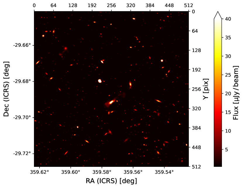
Figure 1: Cutout of 512 square pixels in the SDC1 560 MHz 1000h simulated field. Minimum and maximum cutting values are those used for our object detector, but the image dynamic is not altered.

2 Method

Our method was inspired by the You Only Look Once (YOLO, Redmon et al., 2015; Redmon & Farhadi, 2016, 2018) approach, a regression-based deep learning object detector. While region-based approaches like R-CNN (Girshick et al., 2013) are often considered the most accurate object detectors, regression-based methods present a straightforward single network architecture, making them more compute-efficient at a given detection accuracy. Both families can reach state-of-the-art accuracy depending on implementation details and architecture design. YOLO-like methods are usually preferred for real-time detection applications. In this context, our choice of exploring a YOLO-inspired regression-based approach was driven by i) fewer implementation constraints, ii) a strong emphasis on compute performance considering the upcoming data volume of radio-astronomical surveys, and iii) the single network regression-based structure on which it is easier to add more predictive capabilities.

In this section, we present the main design and properties of our custom object detection method along with necessary general concepts about object detection for non-expert readers. Despite being depicted for an astronomical application, our method remains suitable for general-purpose object detection (Appendix A.8). For clarity, we describe the whole method from scratch, which includes aspects from the classical YOLO implementation and our dedicated modifications. The added or modified elements in comparison to the three first classical versions from the original author, YOLO-V1 (Redmon et al., 2015), YOLO-V2 (Redmon & Farhadi, 2016), and YOLO-V3 (Redmon & Farhadi, 2018) will be mentioned. Still, the more technical and in-depth justifications for these changes are presented in Appendix A. Even though the modifications we brought to the YOLO algorithm are substantial, we still refer to our approach as YOLO-CIANNA in this paper for the sake of simplicity.

The implementation was made inside the custom high-performance deep learning framework CIANNA (Convolutional Interactive Artificial Neural Networks by/for Astrophysicists). The implementation and usage details can be found on the CIANNA wiki pages. For reproducibility purposes, we provide example scripts for training and applying the method to the SDC1 dataset in the CIANNA git repository.

To ease the understanding of the technical parts of the paper for readers unfamiliar with ML terminology, we list a few technical terms we use and the associated descriptions we have for them. The most common ML terms are not defined but can be found in any proper ML textbook or review (LeCun et al., 2015).

• Bounding box: in classical computer vision, the smallest rectangular box that includes all the visible pixels belonging to a specific object in a given image.

• Expressivity: refers to the predictive strength of a network. The higher the expressivity, the more complex or diverse the predictions can be. The expressivity increases with the number of weights and layers in a network.

• Receptive field: corresponds to all the input pixels that can contribute to the activation of a neuron at a specific point in the network. It represents the maximum size of the patterns that can be identified in the input space.

• Reduction factor: the ratio between the input layer spatial dimension and the output layer spatial dimension.

2.1 Bounding boxes for object detection

Our method uses a fully convolutional neural network (CNN) structure to construct a mapping from a 2D input image to a regular output grid of detection units. Each output grid cell represents a small area of the input image with a size that depends on the ratio between the input and the output grid resolutions. Each grid cell is tasked to detect all possible objects whose center is located inside the input region it represents. To characterize an object, we rely on the bounding box formalism that encodes an object as a four-dimension vector composed of the box center and its size ($x,y,w,h$), which are the quantities that the detection units must predict. Our method belongs to the supervised learning approaches, so it relies on a training set composed of images with a list of all the visible objects to be detected. Each object can be encoded as a target bounding box that the detector will be tasked to predict using only information from the input image. This can be done through an optimization process, also called learning, which is an iterative process that aims at minimizing a loss function $\mathcal{L}$, also called an error function, that compares the target boxes with the predicted boxes at the current step. This loss should encompass all the object properties to be predicted. To ease the method description, we first write an abstract loss as

$$\mathcal{L}=\mathcal{L}_{pos}+\mathcal{L}_{size}+\mathcal{L}_{prob}+\mathcal{L}_{obj}+\mathcal{L}_{class}+\mathcal{L}_{param}.$$ (1)

The aim of the Sects. 2.1 to 2.4 is to describe all of the loss sub-parts. Our complete detailed loss function is presented in Sect. 2.7 with Eq. 14.

For now, we only describe the case of a single box prediction per grid cell. The more realistic case of multiple objects per grid cell is presented in Sect. 2.5. To represent a bounding box, each grid cell must predict a 4-element vector ($o^{x},o^{y},o^{w},o^{h}$) that maps to the box’s geometric properties following

$$x =o^{x}+g_{x},$$ (2)

$$y =o^{y}+g_{y},$$ (3)

$$w =p_{w}\mathrm{e}^{(o^{w})},$$ (4)

$$h =p_{h}\mathrm{e}^{(o^{h})}.$$ (5)

Each grid cell is only tasked to position the object center inside its dedicated area, which is obtained using two sigmoid-activated values ($o^{x},o^{y}$). The position of the grid cell in the full image must then be added to obtain the real position of the object, which is expressed by the ($g_{x},g_{y}$) coordinates. The object size is obtained by an exponential transform of the predicted values ($o^{w},o^{h}$) that acts as a scaling on a pre-defined size prior ($p_{w},p_{h}$). This is equivalent to an anchor-box formalism (Ren et al., 2015) as discussed in Sect. 2.5. The corresponding bounding box construction on the output grid is illustrated in Fig. 2.

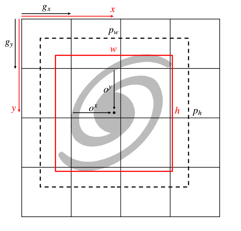
Figure 2: Illustration of the YOLO bounding box representation. The different quantities correspond to Eqs. 2 to 5. The dashed black box corresponds to the theoretical prior ($o_{w}=o_{h}=0$), while the red box represents the scaled network predicted size.

With this formalism, it is possible to construct a network output layer with a $\left<g_{w},g_{h},4\right>$ grid that is capable of positioning and scaling a bounding box for each grid cell. For each prediction-target pair, we use a sum-of-square error to compute the output loss function for center coordinates and sizes (Sect. 2.7). The error is not computed on the sigmoid-activated positions but on the raw output for the sizes after target conversion using $\hat{o}^{w}=\log(w/p_{w})$ and $\hat{o}^{h}=\log(h/p_{h})$. This results in the following loss terms

$$\mathcal{L}_{pos} =\sum_{i=0}^{N_{g}}\mathds{1}_{i}^{match}\left((o^{x}_{i}-\hat{o}^{x}_{i})^{2}+(o^{y}_{i}-\hat{o}^{y}_{i})^{2}\right),$$ (6)

$$\mathcal{L}_{size} =\sum_{i=0}^{N_{g}}\mathds{1}_{i}^{match}\left((o^{w}_{i}-\hat{o}^{h}_{i})^{2}+(o^{h}_{i}-\hat{o}^{h}_{i})^{2}\right),$$ (7)

where the hat values represent the target for the corresponding predicted value, the sum over $i$ represents all the grid cells with $N_{g}=g_{w}{\times}g_{h}$, and $\mathds{1}_{i}^{match}$ is a mask to identify the predicted boxes that have an associated target box (Sect. 2.6). The grid cells that do not contain any object have no contribution to these loss terms. All these elements follow the classical YOLO formalism. We discuss the possible limitations of using bounding boxes to describe astronomical objects in Sect. 5.2.2.

We emphasize that nothing prevents the size of the predicted box from being larger than the area mapped by a grid cell up to the size of the full image. Each grid cell receives information from a large area corresponding to the backbone network receptive field. The receptive fields of nearby grid cells usually overlap, but a target box center can only lie in one grid cell. Due to the fully convolutional structure required for our method, each grid cell represents a localized prediction using identical weights. It is equivalent to having a single detector that scans different regions of the same image but in a more efficient way from a network architecture standpoint. This approach is equivalent to what is done starting with YOLO-V2 but differs from the one introduced in YOLO-V1. More details about the effect of the fully convolutional architecture and the corresponding output grid encoding are provided in Appendix A.1 and A.2.

2.2 Detection probability and objectness score

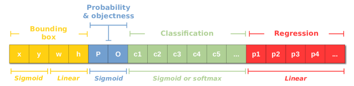
Figure 3: Illustration of the output vector of a single detection unit. The elements are colored by type. The corresponding activation functions are indicated. For multiple detection units per grid cell, this vector structure is repeated on the same axis (Sect. 2.5).

To obtain a working object detector, we not only have to predict bounding boxes but also to evaluate the chances that they indeed contain an object. For this, we add a self-assessed detection probability prediction $P$ to each detection unit, which is constrained during training. This term uses a sigmoid activation and adds a sum-of-square error contribution to the loss. Due to our grid structure, we have one possible box per grid cell. In a context with only a few target boxes in the image, most of the grid cells map irrelevant background regions. During training, we identify the predicted boxes that best represent each target box and attribute them a target probability of $\hat{P}=1$. For all the remaining empty predicted boxes, we associate a target probability of $\hat{P}=0$. To compensate for the probable imbalance between the number of matching and empty predictions, we must define a usually small $\lambda_{void}$ factor to apply to the loss term representing empty predicted boxes. This helps balance the contribution of the two terms. The resulting loss term can be written as

$$\mathcal{L}_{prob}=\sum_{i=0}^{N_{g}}\mathds{1}_{i}^{match}(P_{i}-1)^{2}+\mathds{1}_{i}^{void}\lambda_{void}(P_{i}-0)^{2},$$ (8)

where the sum over $i$ represents all the grid cells, $\mathds{1}_{i}^{match}$ is a mask to identify the predicted boxes that match a target box, and $\mathds{1}_{i}^{void}$ a mask to identify the empty predicted boxes. Due to the stochasticity of the training process, it should result in a continuous probability distribution. At prediction time, the probability is used to identify the grid cells that should contain an object.

This probability definition contains no information about how well the predicted box represents the object. To account for this, we must define a metric that measures the proximity and resemblance between two bounding boxes. The classical metric for object detection is the intersection over union (IoU, Everingham et al., 2010; Lin et al., 2014). It is defined as the surface area of the intersection between two boxes, A and B, divided by the surface area of their union, which is expressed as

$${\rm IoU}=\frac{A\cap B}{A\cup B}.$$ (9)

This quantity takes values between 0 and 1 depending on the amount of overlap. The IoU can then be used to select the best prediction for a given target and quantify the quality of the prediction, but more generally, it can be used to compare two boxes of any kind. This classical IoU is the most commonly used in computer vision, but it presents some weaknesses for astronomical applications. We present a few alternative matching metrics better suited to our application case in Appendix A.4. Because several hyper-parameters of our method depend on this choice of metric, we will use a generic ${\rm fIoU}$ term that can be replaced by the selected matching metric in all the following equations. The default choice for our detector is the distance-IoU (DIoU Zheng et al., 2019), as it includes information about the distance between the center of the two boxes to compare. For all cases where it matters, the selected metric function is linearly rescaled in the 0 to 1 range if it was not already the case.

From this, we add a self-assessed score $O$ called ”objectness” to each predicted box, which is also constrained during training. The objectness is defined as the combination of an object presence probability $P_{obj}$ and the ${\rm fIoU}$ between the predicted box and the target box, expressed as

$$O=P_{obj}\times{\rm fIoU}.$$ (10)

As for the probability, this new term uses a sigmoid activation and adds a sum-of-square error contribution to the loss. The objectness is constrained like the probability by considering that $\hat{P}_{obj}=1$ for prediction-target matches, while $\hat{P}_{obj}=0$ for empty predicted boxes. The difference is the target objectness for the prediction that matches that is defined as $\hat{O}={\rm fIoU}$, following Eq.10, using the ${\rm fIoU}$ of the identified prediction-target couple. The resulting loss term can be written as

$$\mathcal{L}_{obj}=\sum_{i=0}^{N_{g}}\mathds{1}_{i}^{match}(O_{i}-{\rm fIoU})^{2}+\mathds{1}_{i}^{void}\lambda_{void}(O_{i}-0)^{2},$$ (11)

using the same notations as for Eq. 8. We stress that ${\rm fIoU}$ is used as a scalar in this equation. The derivative of the corresponding matching function is not computed for gradient propagation, so $\mathcal{L}_{obj}$ does not contribute to updating the position and size of the prediction. After training, we should obtain a continuous objectness distribution representing a global detection score that includes a self-assessment of the predicted box quality. We note that the classical YOLO formalism only predicts objectness, while YOLO-CIANNA predicts both probability and objectness. They can then be used independently or in association to construct advanced prediction filtering conditions (Sect. 2.8).

With this formalism, we formulate only two statuses for a predicted box, either a match or empty, while in practice, multiple predicted boxes can try to represent the same target simultaneously. This is common if the target box center is positioned at the edge of a grid cell or if the boxes are large. This will be even more common with multiple detections per grid cell (Sect. 2.5). In such a case, only the best-predicted box will be considered a match. The remaining plausible detections are called good-but-not-best (GBNB) predictions. The previous formalism would result in a loss that lowers the objectness of these GBNB predictions, actively forcing relevant features to fade. To prevent this, we define a representation quality threshold ${\rm fIoU}\geq L^{{\rm fIoU}}_{gbnb}$ above which the corresponding boxes are excluded from both $\mathds{1}_{i}^{match}$ and $\mathds{1}_{i}^{void}$ masks. In summary, there are three types of contribution to the loss: i) the best detection for each target updates its box position and size while increasing its probability and objectness, ii) the background boxes lower their probability and objectness, and iii) the GBNB boxes are ignored.

2.3 Classification

The detected box can be enriched with a classification capability. With the classical YOLO formalism, it can be done by adding $N_{c}$ components, corresponding to all the possible classes, to the output vector of the detected boxes. The activation of these components can either be i) a sigmoid for all classes using a sum-of-square error, which allows multi-labeling, or ii) a soft-max activation, which corresponds to exponentiating all the outputs and normalizing them so their sum is equal to 1, with a cross-entropy error. These two options are available in our method. In both cases, only the best detection for each target box updates its classes by comparing the target class vector with the predicted one. There is no contribution to the class loss from both GBNB and background predictions. The resulting loss term for a soft-max activation with a cross-entropy error can be written as

$$\mathcal{L}_{class}=\sum_{i=0}^{N_{g}}\mathds{1}_{i}^{match}\sum_{k}^{N_{C}}\left(-\hat{C}_{i}^{k}\log(C_{i}^{k})\right),$$ (12)

where the sum over $k$ represents all the classes for a given predicted box, and $C_{i}^{k})$ is the corresponding class output for the $k$-th class of the predicted box $i$. We note that classification was not used for the SDC1 as discussed in Sect. 3.1, but it is used for benchmarks on computer vision datasets in Appendix A.8.

2.4 Additional parameters prediction

For astrophysical applications, we usually need to predict source properties like the flux or some geometric properties not described by a bounding box formalism. For this, we propose to add $N_{p}$ components to the output vector of the detected boxes, corresponding to all the additional parameters to predict. The activation of these components is linear with a sum-of-square error contribution to the loss. The respective contribution of these parameters to the loss can be scaled with a set of $\gamma^{p}$ factors. The resulting loss term can be written as

$$\mathcal{L}_{param}=\sum_{i=0}^{N_{g}}\mathds{1}_{i}^{match}\sum_{k=0}^{N_{p}}\gamma^{k}\left(p^{k}_{i}-\hat{p}^{k}_{i}\right)^{2},$$ (13)

where the sum over $k$ represents all the independent parameters for a given predicted box, and $p_{i}^{k}$ is the corresponding parameter output for the $k$-th parameter of the predicted box $i$. We emphasize that it is a strong added value of our YOLO-CIANNA method, allowing it to predict an arbitrary number of added values per detection for any application while preserving the one-stage formalism specific to regression-based object detectors.

2.5 Multiple boxes per grid-cell

With the present definition, the detector output would have a shape of $\left<g_{w},g_{h},(6+N_{c}+N_{p})\right>$, where $g_{w}$ and $g_{h}$ are the grid dimensions, the six static parameters are the box coordinates, probability, and objectness ($x,y,w,h,P,O$), $N_{c}$ is the number of classes, and $N_{p}$ is the number of additional parameters. While the geometric and detection score parameters are always present, both $N_{c}$ and $N_{p}$ are problem-dependent and user-defined. The typical vector for each grid cell with highlighted sub-parts and the corresponding activation functions is illustrated in Fig. 3.

Application cases for which only one object would have to be detected per grid element are uncommon, and high grid resolutions are computationally expensive (Appendix A.2). To overcome this, the classical YOLO approach expands the output vector at each grid cell to contain multiple boxes by stacking their independent vector as a longer 1D vector. The new output shape is then $\left<g_{w},g_{h},N_{b}{\times}(6+N_{c}+N_{p})\right>$, with $N_{b}$ the number of independent boxes predicted by each grid cell. We define an individual size-prior ($p_{w},p_{h}$) for each possible box in a given grid cell, which impacts the size scaling in Eqs. 4 and 5. This definition helps to distribute objects over the available boxes on a given grid cell based on box sizes and shapes. The prior list is the same for each grid cell due to the fully convolutional network backbone required for our method (Appendix A.1). In the latter, we refer to these independent predictive elements as ”detection units”. For example, a network set capable of predicting up to 6 independent boxes per grid cell is composed of 6 detection units. Some detection units can have the same size prior, but they still represent independent predictions.

Because scales or shapes are unlikely to be evenly represented in the training sample, the detection units should adapt their positive-to-negative detection ratio to rebalance their probability and objectness distribution (Sect. 2.2). For this, a $\lambda_{void}^{b}$ factor is defined for each detection unit. These factors must be adjusted so the objections and probability responses are sufficiently similar for all detection units to be compared during prediction filtering (Sect. 2.8).

2.6 Target-Prediction association function

With multiple box predictions per grid cell, it is necessary to establish a clear process to decide which detection unit should be associated with each target box. Inside our YOLO-CIANNA method, we introduce a new prediction-aware association process. Our approach is very different than the one used in the classical YOLO formalism, which only uses the size priors to define the theoretical best matches. Our method proposes solutions to identified limitations of the classical YOLO for astronomical applications, especially regarding images with a high density of small objects. An in-depth comparison of our approach with the classical YOLO is presented in Appendix A.3.

The main objective of our association process is to find the best target-prediction pairs regarding a specific ${\rm fIoU}$ matching metric. We start by setting $\mathds{1}^{void}=1$ for all detection units. Then, we identify all predicted boxes that are a good enough representation of at least one target regarding our ${\rm fIoU}\geq L^{{\rm fIoU}}_{gbnb}$ threshold. This comparison is made for all detection units and all targets regardless of their center position. All objects that respect this criterion are removed from $\mathds{1}^{void}$. The rest of the association algorithm aims to find the ”best match” for each target box through an iterative process. First, matching scores for all possible target-prediction pairs in a grid cell are stored in a scoring matrix. Then, the best current score in the matrix is used to define a new target-prediction pair that is added to the $\mathds{1}^{match}$ mask and removed from $\mathds{1}^{void}$ if it was not already the case. The full row and column corresponding to the target and detection unit of the best match are masked in the score matrix. This search process is repeated until the score matrix is empty or fully masked. As presented in Sect. 2.2, the best match associations contribute to all sub-parts of the loss, while the detection units that remained in $\mathds{1}^{void}$ contribute only to the probability and objectness following Eq. 11. The remaining GBNB detection units not being part of either $\mathds{1}^{match}$ or $\mathds{1}^{void}$ do not contribute to the loss.

To account for edge cases, size imbalance, or training difficulty, we added several specific refinements inside our custom YOLO-CIANNA association process, which we detail in an appendix section dedicated to advanced subtleties of our method (Appendix A.6). The global association function algorithm is presented in Fig. 4 in a way that separates the simplified association process and the advanced association with refinements.

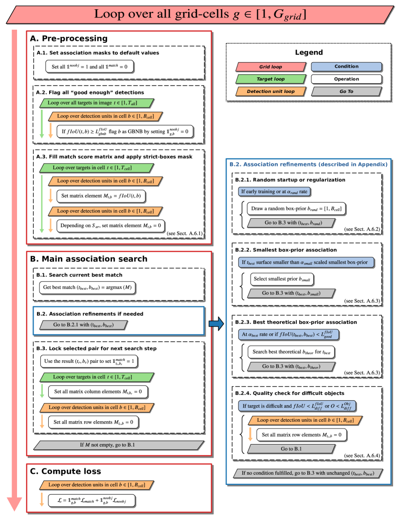
Figure 4: Summary of the target-prediction association algorithm of YOLO-CIANNA. All the steps are done independently by each grid cell. All the elements are executed in order from top to bottom, with the left column representing the general case for the association. All the refinements corresponding to the B.2 block are described in Sect. A.6.

2.7 YOLO-CIANNA complete loss function

Depending on the application, it might be useful to balance the relative importance of the predicted quantities. For example, high precision on the predicted size might not be necessary when detecting small objects, while center position becomes the main factor of prediction quality. Following the classical YOLO approach, we have loss scaling factors for the box position $\lambda_{pos}$, the box size $\lambda_{size}$, the probability $\lambda_{prob}$, the objectness $\lambda_{obj}$, the classes $\lambda_{class}$, and the extra parameters $\lambda_{param}$.

While loss scaling balances the general final importance of each predicted quantity, it does not allow the network to guide its expressivity regarding its current prediction dynamically. For example, adjusting the predicted class of a detection unit that does not yet properly position or detect the corresponding object is irrelevant, and it might even reinforce wrong features or add noise to the training. To add this capability, we enriched the custom loss of our YOLO-CIANNA method with prediction quality limits over some predicted properties. While the position and the size are always updated for a match, we added quality limits for the objectness $L^{{\rm fIoU}}_{O\_good}$, the probability $L^{{\rm fIoU}}_{P\_good}$, the classification $L^{{\rm fIoU}}_{C\_good}$, and the extra-parameters $L^{{\rm fIoU}}_{p\_good}$. Each loss sub-part is set to zero if the current ${\rm fIoU}$ between the target and predicted boxes is below its specific quality threshold.

This quality limit principle, combined with other association refinements, results in what we call a ”cascading loss” that varies during training to guide the network expressivity toward the important aspects, not adjusting currently irrelevant properties. A complete description of this process and the effect it has on training performances and loss monitoring is given in Appendix A.7. With all the previously introduced elements, we can define our complete YOLO-CIANNA loss function for one image as

$$\begin{split}\mathcal{L}=&\sum_{i=0}^{N_{g}}\sum_{j=0}^{N_{b}}\mathds{1}_{ij}^{match}\begin{aligned} \Biggl{(}&\lambda_{pos}&&\left[(o^{x}_{ij}-\hat{o}^{x}_{ij})^{2}+(o^{y}_{ij}-\hat{o}^{y}_{ij})^{2}\right]\\ +&\lambda_{size}&&\left[(o^{w}_{ij}-\hat{o}^{h}_{ij})^{2}+(o^{h}_{ij}-\hat{o}^{h}_{ij})^{2}\right]\\ +&\lambda_{class}&&\mathds{1}_{ij}^{C\_good}\sum_{k}^{N_{C}}\left(-\hat{C}_{ij}^{k}\log(C_{ij}^{k})\right)\\ +&\lambda_{param}&&\mathds{1}_{ij}^{p\_good}\sum_{k}^{N_{p}}\gamma^{k}\left(p^{k}_{ij}-\hat{p}^{k}_{ij}\right)^{2}\\ +&\lambda_{prob}&&\mathds{1}_{ij}^{P\_good}\left(P_{ij}-1\right)^{2}\\ +&\lambda_{obj}&&\mathds{1}_{ij}^{O\_good}\left(O_{ij}-{\rm fIoU}_{ij}\right)^{2}\Biggl{)}\end{aligned}\\ +&\sum_{i=0}^{N_{g}}\sum_{j=0}^{N_{b}}\mathds{1}_{ij}^{void}\lambda_{void}^{j}\begin{aligned} &\Biggl{(}\lambda_{prob}\left(P_{ij}-0\right)^{2}+\lambda_{obj}\left(O_{ij}-0\right)^{2}\Biggl{)}.\end{aligned}\\ \end{split}$$ (14)

In this equation, in addition to the already defined parameters, the first sum runs over all the elements of the output grid for a single image $N_{g}$, and the second sum runs over all the detection units in a grid cell $N_{b}$. All the values with a hat represent the targets for the corresponding predicted values, and the $\mathds{1}_{ij}^{X\_good}$ are masks that identify the predicted boxes that respect the prediction quality limit of each sub-parts. This loss is written for a classification based on a soft-max activation with a cross-entropy error, but a sigmoid activation with a sum-of-square error is also available in our implementation.

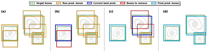
Figure 5: Illustration of the NMS process in a given image. The dashed boxes are the target, and the solid boxes are the predictions. The line widths of the boxes are scaled on their respective objectness score. The colors indicate the state of the box in the NMS process at different steps. Frame (a) represents the targets and the raw network predictions that remain after the objectness filtering. Frames (b) and (c) represent two successive steps of the NMS process with a different best current box. Frame (d) represents the remaining boxes after completion of the NMS.

2.8 Prediction filtering and non-maximum suppression

We expect a properly trained detector to order its predictions by quality based on the predicted objectness score for each detection unit. The raw detector output is always a static list of boxes of size $\left<g_{w},g_{h},N_{b}{\times}(6+N_{c}+N_{p})\right>$ regardless of the input content. Consequently, the predicted boxes must be filtered based on their objectness score to remove those that are unlikely to represent an object. By design, the number of actually detectable objects in the image should be low compared to the total number of detection units in the grid. Therefore, most of the predicted boxes belong to the background type with a low objectness score.

While the continuous objectness score is the best direct representation of the detector’s inner workings, it is incompatible with some final metric that needs a list of considered ”good” detections. Visualizing the predicted boxes also requires filtering to preserve only the plausible detection. In such cases, an objectness threshold can be used to remove low-confidence detections. This is usually done on a validation or test dataset not used for training but for which the targets are known. The threshold can be optimized to maximize a detection metric on this test dataset.

The main difficulty is that all detection units have fitted their objectness independently. Due to the fully convolutional structure of the network, a given detection unit represents the same objectness fitting over the full grid, meaning that the same threshold can be used. On the contrary, the predicted objectness between two independent detection units is not comparable as it depends on the type and frequency of targets associated with each of them at training time. The classical solution is to fit an individual objectness threshold for each of them. However, it considers that predictions from different detection units are independent, which is not true for most applications. Still, fitting a per-detection-unit objectness threshold removes the vast majority of false positives. To achieve the best results, the objectness regimes must be homogenized between the different detection units from the start by adjusting the individual $\lambda_{void}^{b}$ factors (Sect. 2.5). While this is mainly an empirical and iterative process, the main principle is to balance the ratio between detection and background cases based on how the objects from the training sample are expected to distribute over the detection units.

With most false positives removed, there can still be multiple high-objectness predictions that represent the same object. To preserve only the best-detected box for each object, we use a classical post-processing step called non-maximum suppression (NMS, Felzenszwalb et al., 2010; Girshick et al., 2013). It consists of an iterative search for the box with the highest objectness score in the image to remove all the overlapping predicted boxes. To consider that there is an overlap, the two boxes must verify ${\rm fIoU}>L^{{\rm fIoU}}_{NMS}$ with the ${\rm fIoU}$ being computed between the two predicted boxes. All boxes with a lower objectness score than the highest-scoring box are removed, and the best box is added to a static prediction list. This process is repeated until no boxes are left in the raw-prediction list. It is illustrated in Fig. 5.

The NMS is done regardless of what detection unit generated the predicted boxes, demonstrating that they are not independent as they can remove each other based on their respective objectness. This is one of the main reasons to force all detection units to have similar objectness distributions. The detection quality can only be evaluated after the NMS, so searching for the best $\lambda_{void}^{b}$ factors is dependent on the $L^{{\rm fIoU}}_{NMS}$ and respectively.

3 Dataset description and network training

In this section, we present the main aspects of the SDC1 data along with the expected products and the associated metrics. A complete description of the SDC1 challenge and its data products can be found in Bonaldi et al. (2021), while the underlying T-RECS simulation is detailed in (Bonaldi et al., 2019). We also present the pre-processing of the data to construct our training sample. From this, we describe our best-performing network architecture and specify the corresponding setup and hyper-parameters for our YOLO-CIANNA detector.

3.1 Sub-challenge definition

The SDC1 is a source detection and characterization task in simulated SKA-like data products (Sect. 1) that comprises nine 4GB images (three frequencies, with three integration times each) of the same field. The SDC1 is only modestly challenging regarding data volume, especially compared to the SDC2 with its 1TB data cube. Still, it represents significant challenges for detection methods in many other aspects. All the images have the same size of 32768 square pixels. As the frequency increases, the angular resolution improves while the field of view reduces. Therefore, images at different frequencies only partially overlap, meaning that the problem to solve varies with the position in the field. In addition, the number of detectable sources varies significantly with the integration time and frequency (Table 2 in Bonaldi et al., 2021). We also note that all the images are considered noise-limited, even at the highest 1000h integration time. As a benchmark for our YOLO-CIANNA, we chose to use the 560 MHz - 1000h image due to its larger field of view, higher total number of sources, and larger source density per square pixel. This image is an appropriate benchmark for our YOLO-CIANNA method, representing a difficult astronomical detection context with a high dynamic and a high density of small sources with occasional blending. While our method could technically work for the other SDC1 images, it would not be more informative regarding its capabilities. The consequences and limits of this choice are further discussed in Sect. 5.2.1.

In the original challenge, participating teams were provided a True catalog for a small fraction of the image. This was supposed to facilitate method development and tuning but also allow training of supervised ML approaches. At the time, the full underlying True catalog was unavailable, and the teams had to submit their result to a remote scoring service. After the challenge, the organizers released the full True catalog, the scoring code in open source (Clarke & Collinson, 2021), and the submitted source catalogs from the participating teams. This allows anyone to either reproduce the challenge conditions or to use the full simulated field for other purposes. In this study, we use only the training catalog to constrain our detector to benchmark our method comparatively to other approaches. We then use the full True catalog only to present an in-depth analysis of our detector performances. Since the scorer allows individual image scoring (for all frequencies and exposure), we can produce a detection catalog for the 560 MHz - 1000h image that is directly comparable to other team submissions during and after the challenge.

3.2 Image and source catalog description

The 560 MHz - 1000h image has a field of view of $5.5$ square degrees, which contains the primary beam out to the first null. It has a full size of 32768 square pixels, a pixel size of $0.6$ arcsec, and an imaging resolution in the Gaussian approximation of $1.5$ arcsec full width at half-maximum. The noise level at this exposure and frequency is estimated at $2.55{\times}10^{-7}$ $\mbox{Jy}.\mbox{beam}^{-1}$. An example sub-field of 512 square pixels from this image is presented in Fig. 1. The simulated image contains no systematic instrumental effects like calibration, pointing, or deconvolution errors, making it unrealistically clean (Sect. 5.3). The image is not primary-beam corrected, but the corresponding primary beam image is available as ancillary data. With this setup, the instrument sensitivity decreases on the edges, but it preserves a uniform noise level over the full field. While we could convert the image to a beam-corrected one, it is better for the detector to work on the constant noise image and to detect sources from their apparent brightness (Sect. 3.5). The apparent flux of a source can be obtained by multiplying the flux from the True catalog by the interpolated primary beam value at the source’s central position.

The SDC1 challenge task is to detect and characterize the sources. The expected parameters for each source are the coordinates ($RA$, $Dec$), the integrated source flux $f$, the core fraction $c_{f}$ if different from zero, the major and minor axis ($Bmaj,Bmin$), the major axis position angle $PA$, and a classification $C$ (one of AGN-steep, AGN-flat, or star-forming galaxy). The provided True catalog provides all these properties for each source, allowing the training of supervised methods. From Sect. 5.3 in Bonaldi et al. (2021), the classification is considered difficult as it is only feasible on the fraction of the field where all frequencies are available. For this reason, we focused on getting the best performances on a detection and characterization problem only.

3.3 SDC1 scoring metric

The first element of the scorer is a match criterion. Due to source density, relying only on the central positions of the sources to establish proper matches is not enough. The SDC1 scorer uses a combination of the position, the size, and the predicted flux accuracies to represent a global matching score defined as

$$E_{tot} =\sqrt{E^{2}_{pos}+E^{2}_{size}+E^{2}_{flux}}\text{, with}$$ (15)

$$E_{pos} \propto\sqrt{(x-\hat{x})^{2}+(y-\hat{y})^{2}}/\hat{S}^{\prime}\text{,}$$ (16)

$$E_{size} \propto\left|S-\hat{S}\right|/\hat{S}^{\prime}\text{, and}$$ (17)

$$E_{flux} \propto\left|f-\hat{f}\right|/\hat{f},$$ (18)

where the true values from the catalog are indicated with a hat, ($x,y$) is the central coordinates in pixels corresponding to ($RA,Dec$), $S$ is the average value of $Bmaj$ and $Bmin$, $S^{\prime}$ is the largest axis convolved with the synthesized-beam, and $f$ is the source flux. We note that the difference between $S$ and $S^{\prime}$ is present in the scorer code but not specified in Bonaldi et al. (2021) or the challenge documentation. To prevent false detections due to the high source density, the scorer defines a strict match threshold value for $E_{tot}$. Each sub-part of the error is normalized to a value considered representative of a $1\sigma$ error. In the scorer, the normalization coefficients are set to $0.93$ for the position, $0.36$ for the flux, and $4.38$ for the size, all using the catalog units defining a global $1\sigma$ error. These individual limits were obtained by fitting the distribution of the corresponding values on the combination of all the submitted catalogs at the challenge time. A match is then defined if $E_{tot}<5\sigma$, which was optimized to reduce the average random association chance of all submitted catalogs below 10 percent. We note that the scorer distinguishes false detection into two categories: either ”False” if there is no target source closer than 1.5 times the predicted size convolved with the beam, or ”bad” if it passes this distance limit but has a too high $E_{tot}$.

From a list of identified matches, a global score that captures both the detection and the characterization has to be defined. The SDC1 scorer attributes a score of up to one point for each match depending on its characterization quality and penalizes every false detection with a strict minus one point. The characterization evaluation is decomposed into seven individual sub-scores that all respect the following scoring rule (based on the scorer code) for a single source

$$s_{i}^{j}=\min{\left(1,\frac{T^{j}}{E_{i}^{j}}\right)},$$ (19)

where $j$ represents the sub-score part and $i$ a single source from the match list, $T^{j}$ is a threshold for this sub-score part, and finally, $E_{i}^{j}$ and $s_{i}^{j}$ correspond to the error term and the final sub-score part for this source. We list all the sub-score parts and their corresponding $E^{j}$ function and $T^{j}$ values in Table 1, and we illustrate the typical score as a function of the error regarding a given threshold value in Fig. 6.

We note that all of the sub-part error functions are based on a relative error, which has an asymmetric behavior. When overestimating the value, the error can rise infinitely, while underestimating a strictly positive prediction will never lower the relative error below -1. The issue is that these errors are associated with symmetric score response functions. As a consequence, the score is likely to be higher when underestimating the predictions, which is unlikely to naturally happen on quantities that have minimum practical values due to instrumental limits like the $flux$, $Bmaj$, and $Bmin$. While the effect is minor for the sub-part scoring, we note that for the matching criteria, it will result in excluding properly detected faint sources for which the noise caps the minimum predictable flux. This aspect is discussed in more detail in Sects. 4.5 and 5.1.

The final score for a given source and the average sub-part score for all sources are

$$s_{i}=\frac{1}{7}\sum_{j}^{7}s_{i}^{j}\quad\text{ and }\quad\bar{s}^{j}=\sum_{i}^{N_{match}}s_{i}^{j}.$$ (20)

To obtain the full SDC1 score, there is a scaling between the different frequencies and integration times. However, since we limit this study to a single image, there is no need for these definitions. The average source score for matching sources is

$$\bar{s}=\frac{1}{N_{match}}\sum_{i}^{N_{match}}{s_{i}},$$ (21)

and the final SDC1 score for a single image is then

$$M_{s}=\sum_{i}^{N_{match}}{s_{i}}-N_{false}.$$ (22)

When scoring a submitted catalog, the training area is excluded, so detection performances are evaluated only for examples that were not used to constrain the detector.

Table 1: Error functions and threshold values for all sub-scores.

Sub-part	Error function $E^{j}$	Threshold $T^{j}$
Position	$\sqrt{(x-\hat{x})^{2}+(y-\hat{y})^{2}}/\hat{S}^{\prime\prime}$	0.3
Flux Density	$\left|f-\hat{f}\right|/\hat{f}$	0.1
Major axis	$\left|Bmaj-\hat{Bmaj}\right|/\hat{Bmaj}$	0.3
Minor axis	$\left|Bmin-\hat{Bmin}\right|/\hat{Bmin}$	0.3
Position angle	$\left|PA-\hat{PA}\right|$	10.0
Classification	$1\text{ if }C=\hat{C}\text{, }0\text{ otherwise}$
Core fraction	$\left|cf-\hat{cf}\right|/0.75$	0.05

Note: $\hat{S}^{\prime\prime}$ is the target source average size convolved with twice the synthesized beam size, which is different from $\hat{S}^{\prime}$

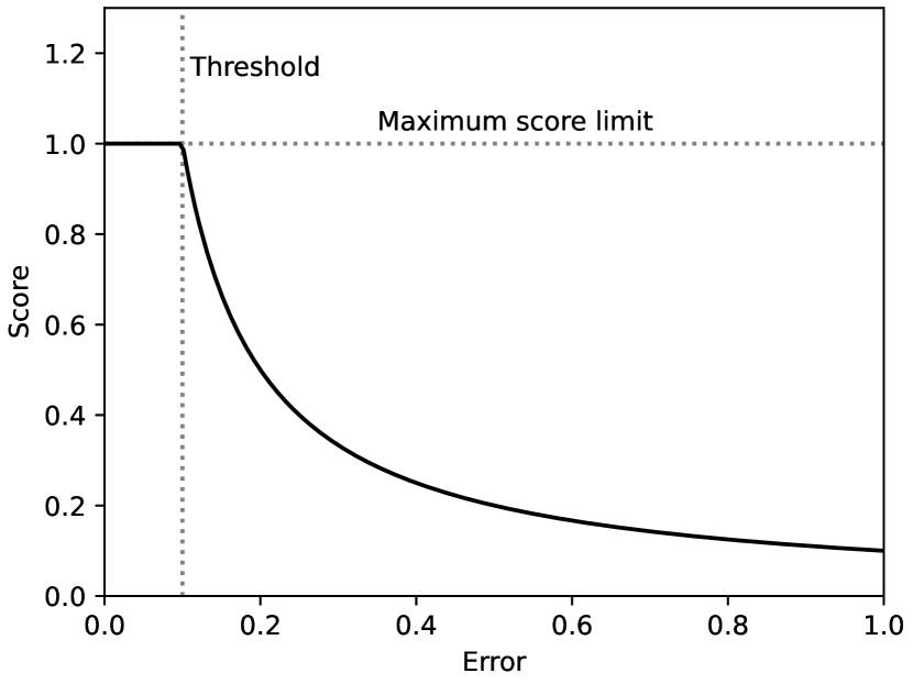
Figure 6: Generic scoring function response for a source parameter with $T=0.1$ as a function of the prediction error.

3.4 Selection function

The full simulation of the SDC1 contains more than five million sources. Due to the simulated noise, only a fraction of these sources are detectable in the image. In Bonaldi et al. (2021), they estimated that only around 758000 sources are above the noise level by $5\sigma$ in the 560 MHz - 1000h image. This construction is problematic for supervised ML methods as they are very sensitive to wrong labeling during training. For an object detector, it goes two ways: i) if a source is detectable but not labeled as a target box, the network lowers the detection objectness of all predicted boxes that try to detect similar sources; ii) if there is a target box for a source that the network is incapable of detecting, it increases the objectness of non-representative features, likely background noise. Consequently, to achieve good detection performances, we must construct a training sample that is both complete and pure regarding the detectability of the sources it contains. For this, we defined a selection function based on the source properties of the provided True-catalog.

Our selection function combines the apparent source flux $f_{a}$ in Jy, and a surface brightness estimate $S_{b}$ computed as

$$S_{b} =f_{a}/(W_{pix}\times H_{pix})\text{, where}$$ (23)

$$W_{pix} =(2/P_{s})\times\max{(1.2,Bmaj)}\text{ and }$$ (24)

$$H_{pix} =(2/P_{s})\times\max{(0.6,Bmin)}.$$ (25)

The size saturation values are in arcsec and correspond to a two and one-pixel size, respectively, and $P_{s}$ represents the pixel size in arcsec used to obtain the box size in pixels. The apparent source flux is obtained by multiplying the integrated source flux by the interpolated primary beam value at the central coordinates of the source. The selection function to keep a source in our training sample is then defined as

$$\cases{S}_{b}>1.0\times 10^{-7}&\text{if }f>=7.0\times 10^{-6}\\ S_{b}>2.5\times 10^{-7}\text{ \& }f>1.65\times 10^{-6}\text{otherwise}.{}$$ (26)

We represent these cuts over a 2D histogram of the source surface against apparent flux for the training area in Fig. 7. In this figure, the top left patchy distribution corresponds to steep spectrum AGN. The flat spectrum AGN and star-forming galaxies follow the same principal distribution but are strongly unbalanced with only a few flat spectrum AGN. In practice, both types of AGNs are mostly undetectable with the 560 MHz - 1000h setup and, therefore, are strongly underrepresented after our selection function. This also contributes to the identified difficulty of the classification task in the SDC1 result paper (Sect. 5.3 in Bonaldi et al., 2021). The hard cut visible at the bottom left of the distribution results from the prefiltering done directly by SKAO, which is characterized by the ”selected” flag in the training catalog. Due to our size clipping, most of the surface range of this space is collapsed at a minimum surface, represented by the dotted grey line. We observed that lower clipping limits tend to increase the number of non-visible objects that pass the selection.

We represent the effect of our selection function regarding the apparent flux distribution in Fig. 8. We also illustrate the effect of our selection on a small field in Fig. 9. We see that it misses some apparent compact signals, which can result from several effects: i) the local noise contribution can increase the perceived apparent flux of a very faint source, ii) it can correspond to blended faint point sources that add their flux at the same location, and iii) it can also be a bright, compact part of a globally large and faint source that does not respect the surface brightness limit. Regardless of their origin, these non-labeled compact signals will likely confuse the network training, but properly handling them would require a more complex selection function. We will see in Sects. 4.2 and 4.5 that the detector can still detect these types of sources, but since the perceived flux will not match the True catalog content, they are likely to be considered as false detections. We tried to adapt the selection process and our threshold values, but the current formulation produced the best results. We also tried to define our surface brightness using a more common astronomical size definition by convolving the $Bmaj$ and $Bmin$ with the synthesized beam. Still, it always resulted in lower detector scores after training.

In Appendix C.2, we discuss an alternative way to construct this function iteratively using the prediction of a naively trained network to evaluate the detectability of the sources.

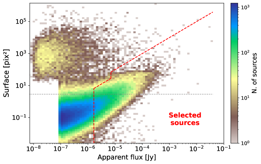
Figure 7: 2D histogram of the source surfaces as a function of their apparent flux. The surface is equivalent to $S_{b}$ but without minimum size clipping. The dotted grey line indicates the saturated minimum surface with clipping. The red dashed line represents our selection function.

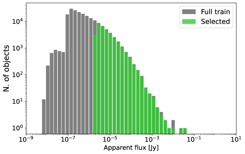
Figure 8: Source apparent flux distribution histogram in log scale and using log-bins for the True catalog of the training region and the training catalog after the selection function.

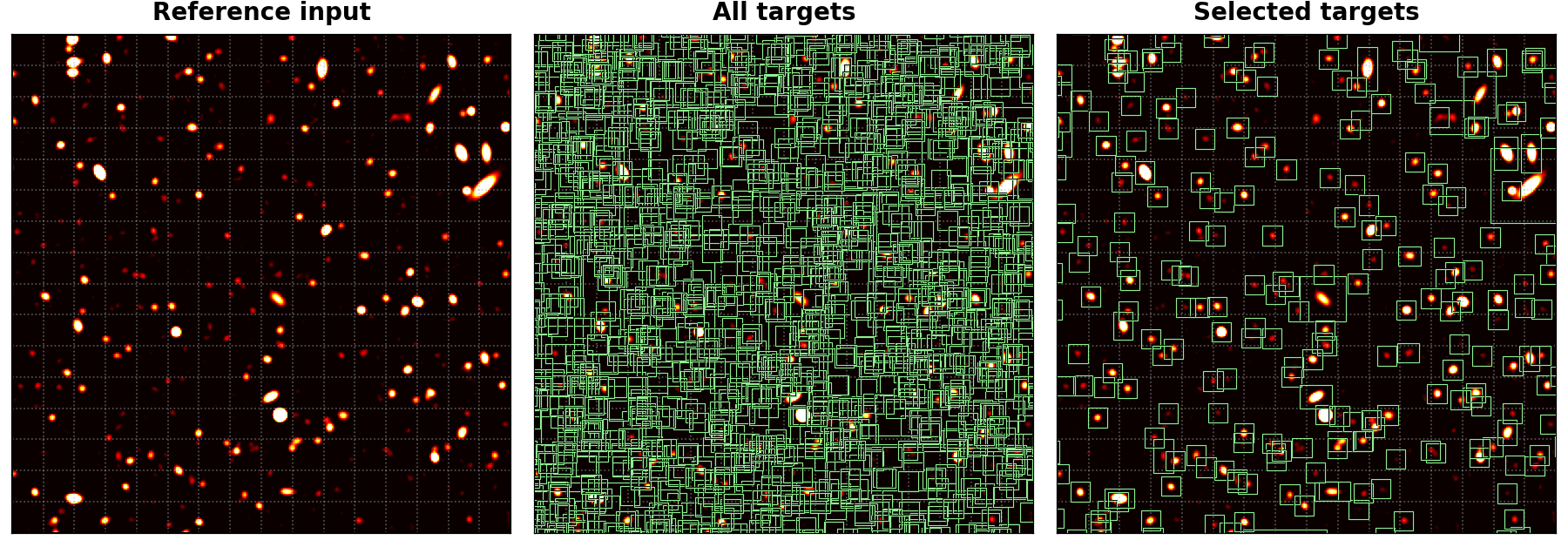
Figure 9: Illustration of the selection function over a typical input field. The background image represents an identical $256{\times}256$ input patch in all frames, centered on $RA=0.1$ deg, $Dec=-30.2$ deg, using the re-normalized input dynamic but saturated at half the maximum value to increase visual contrast. The displayed grid corresponds to the detector output grid mapping for a network reduction factor of 16. The left frame is provided as an image reference, the middle frame represents all the target boxes from the True catalog, and the right frame represents the remaining target boxes after our selection function.

3.5 Training area

Using the challenge setup, the provided training area only spans a small part of the image center, corresponding to a surface of about $0.308$ square degree. The associated training catalog contains 190552 sources (using the pre-defined ”selected” flag), corresponding to roughly $3.6\%$ of the sources from the full True catalog. Applying our custom selection function to this region drops the number of sources to 33813. Due to the effect of the primary beam sensitivity over the image field, the central area is not a good representation of other parts of the image. The learned features and context awareness of a detector trained on this region are unlikely to generalize properly in other parts of the image. We represent the distribution of sources that pass our selection function based on apparent source brightness for the full image field using the full True cat in Fig. 10. The footprint of the primary beam sensitivity is clearly visible. The provided training area corresponds to the red box. A more suited training area definition could have been a narrow band over a full radius of the image, which we explore in Appendix C. To mitigate the generalization issue while still following the original challenge definition, two classical approaches would be to constrain the detector to be flux agnostic and only perform morphological detection or to reject all sources outside a given radius from the image center.

We propose another approach that uses other regions of the image without adding any target sources. We observed that detecting an object above a given radius from the image center becomes very unlikely. From this, we added two ”noise only” regions to our training sample that are sufficiently far from the image center to be considered devoid of any detectable source. We selected two rectangular regions of identical width and height of 2000 and 5600 pixels, respectively, that are both vertically centered in the image but on opposite sides horizontally with a margin to the image edge of 250 pixels (Fig. 10). These regions lie between the primary beam’s main lobe and the first sidelobe. We acknowledge that the emptiness assumption is not completely true for multiple reasons and that it necessarily results in some non-labeled visible sources. Still, including cutouts from the ”mostly noise” context in the training sample is vastly beneficial regarding global detector performances. Training examples are mostly drawn randomly in the default training area but at a low $5\%$ rate in one of the two noise-only regions. This forces the network to understand the dynamic of parts of the image where it is not expected to detect anything. We observed that networks trained with this process can interpolate between the two regimes and provide much better results for the full image without manually excluding difficult regions. Compared to training on the default region only, the best achievable challenge score is increased by more than 10% with this approach.

Figure 10: 2D histogram of the central coordinates of the sources from the full True catalog that pass our selection function. The red box indicates the default SDC1 training area, and the orange boxes indicate our additional noise-only regions.

3.6 Network backbone architecture

As introduced in Sect. 2.1, our method requires a fully convolutional neural network backbone to create a mapping from a 2D input image to a regular output grid. Efficient neural network architectures can be built by stacking convolutional layers while progressively reducing the spatial dimension to filter the relevant information and construct higher-level representations of the input content, forming a CNN (Simonyan & Zisserman, 2014; LeCun et al., 2015). With a fully convolutional structure, the last layer is responsible for encoding the output grid of the detector. Its spatial dimension represents the output grid, and the filters encode all the output vector elements for each grid cell. It also results in the output grid size being controlled by the reduction factor of the backbone network, which corresponds to the total spatial reduction of the network from its input to the output. The properties of a fully convolutional architecture and its impact on our method design are further detailed in Appendix A.1.

With a fully convolutional architecture, we could technically use any input dimension (Appendix A.1) and even use different input sizes for training and prediction. In this section, we consider the input size to be $256{\times}256$ pixels (Sect. 3.8). Regarding the reduction factor, we found that a value of 16 resulted in the best detection accuracy, which means that the training output grid is composed of $16{\times}16$ cells. Considering the source density of the 560 MHz - 1000h image, each grid cell has to detect multiple sources, which was the motivation behind most of the adjustments we made to our association process in comparison to the classical YOLO (Appendix A.3).

At this point, it would be tempting to adopt the classical YOLO-V2 architecture, darknet-19 (Redmon & Farhadi, 2016), as we successfully used it with CIANNA for other contexts with our custom association process (Appendix A.8). We discuss this possibility and explain why it would lead to poor performances in Appendix B. Instead, we meticulously explored increasingly complex custom backbone architectures. We specifically looked for an architecture that is both compute-efficient and capable of achieving high detection accuracy. An illustration of our final architecture is presented in Fig. 11.

Our architecture is based on a few educated guesses, but it also requires exploration through score optimization. We first note that the spatial dimension is always reduced by convolution operations instead of pooling operations. In comparison to pooling operations, it helps preserve the apparent flux information, and it better represents continuous objects with no sharp edges. The first layer has larger filters to grasp more continuous luminosity profiles, while the second layer performs a local compression (both spatially and in the number of filters), mainly acting as a local noise filter. Then, for a few layers, we progressively increase the number of filters while decreasing the spatial dimension at a rate that maximizes computation performances. After the 7th layer, we start alternating large layers with $3{\times}3$ filters and smaller layers with $1{\times}1$ filters, which is typical of the YOLO darknet architecture. This structure alternates searches for local spatial coherency with representation compressions. It improves compute performance and reduces the global number of parameters compared to a more classical stacking of identically sized $3{\times}3$ layers. We also note that our third spatial-dimension reduction layer (8th layer in global) is also considered a compression layer. The second last layer has a 25% dropout rate, which is used for regularization (Srivastava et al., 2014).

Following what is done in the darknet-19 architecture, we tested adding group normalization (GN, Wu & He, 2018) at various places in the network, but it almost always degraded the best achievable score by a few percent (Appendix B). This is likely because this type of normalization tends to lose the absolute values of the input pixels, making it more difficult to predict the flux accurately. Since the normalization is made on the full spatial dimension, it might also affect the dynamic in a way that makes faint sources more difficult to detect. The only place where GN produces a beneficial effect is near the end of the network, after the last spatial correlation, at a point where the flux value is likely fully re-encoded in the high-level features. This specific normalization layer has several beneficial effects, including a speed up and stabilization of the training process and also a small improvement of the best achievable score of about $2\%$.

The full architecture contains 17 convolution layers for a total of around 12.62 million weights. We note that almost 76% of these weights are concentrated at the network’s end in the connections between layers 14 to 16. With this architecture, the receptive field for a given grid cell at the output layer is 100 pixels. This means that each detection unit will only capture information in an input region with a typical diameter of 100 pixels center on its grid cell. It limits both the maximum size of the sources that can be detected with this architecture and the context windows that each detection unit can use. We discuss the limits of the current network structure and potential architecture improvements in Sect. 5.2 and Appendix A.8.1.

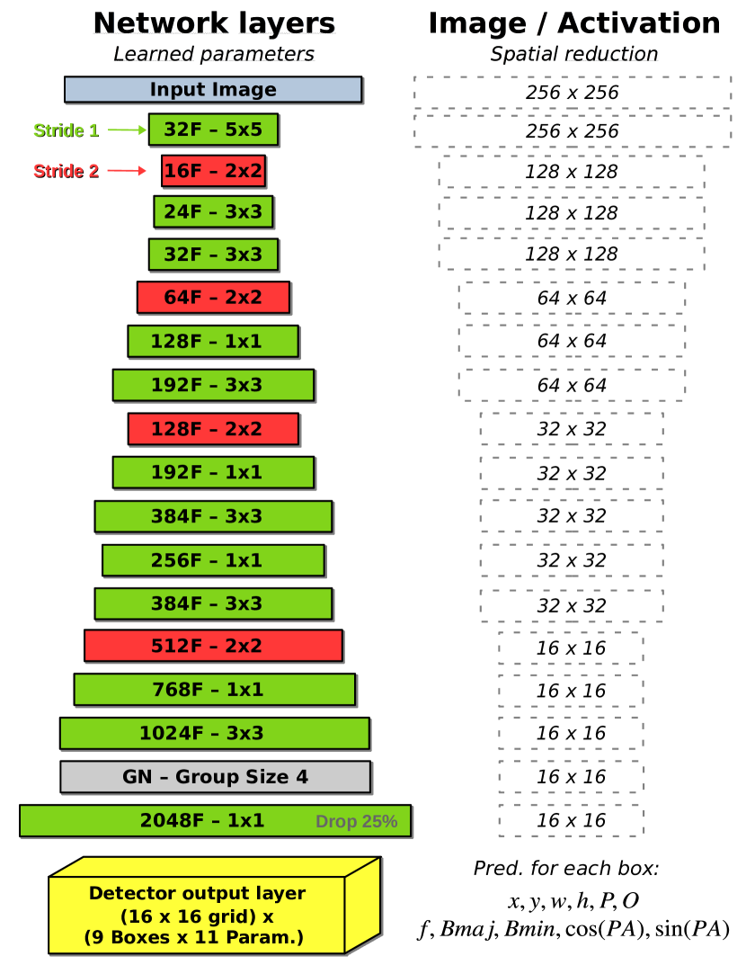
Figure 11: Illustration of our final CNN backbone architecture. The left column provides the layer structural properties, while the right column indicates the spatial output dimension for each layer starting from a $256{\times}256$ input size. The input image is on the top, and layers are stacked in order vertically. The width of a layer represents its number of filters. The green color indicates a layer that preserves the spatial dimension, while the red color indicates a reduction. The full output dimensions of the detector grid output are reminded at the end with the list of the predicted parameters for each box.

3.7 YOLO-CIANNA configuration

3.7.1 Input normalization

Input normalization is a critical requirement to obtain good detection performances in our specific context. This aspect is particularly difficult for astronomical images due to the very high dynamic range. Everyday-life images are usually encoded using three 8-bit integers, resulting in 256 possible values for each color. Converting an astronomical image to a similar format would induce a huge information loss. We found that 16-bit floating-point quantization was sufficient for the SDC1 image after other input transformations, but some astronomical datasets are likely to require 32-bit floating-point encoding. It is also useful to offset the raw dynamic to represent the low flux regime better. In our case, we redefine our minimum and maximum values as $min_{p}=4{\times}10^{-7}\,\mbox{Jy}.\mbox{beam}^{-1}$ and $max_{p}=4{\times}10^{-5}\,\mbox{Jy}.\mbox{beam}^{-1}$, and apply a scaled hyperbolic tangent for all pixel values. Our full renormalization can be summarized as

$$p_{i}^{\prime}=\tanh{\left(3\times\frac{p_{i}-min_{p}}{max_{p}-min_{p}}\right)},$$ (27)

where $p_{i}$ is the raw pixel value in $\mbox{Jy}.\mbox{beam}^{-1}$ clipped with the two limits, and $p_{i}^{\prime}$ is the pixel value as it is presented to the network. This normalization remaps all input data in the 0 to 1 range and grants most of this range to low signal values using an almost linear regime to maximize the available information to distinguish the sources from the noise. The counterpart is a flattening of the dynamic for high fluxes, but bright sources require less accuracy on the pixel values to obtain a good relative flux estimate.

3.7.2 Detection units settings

To configure our detection units, we must first define our target boxes. The True catalog does not contain the necessary information to define them in the classical computer vision way. Instead, we define our boxes as centered on the source central coordinates and with a size that is scaled on its major and minor axes. For each target source, we first define a rectangular box with $\hat{w}_{PA=0}=2\times Bmaj$ and $\hat{h}_{PA=0}=2\times Bmin$ corresponding to $PA=0$. This box is then rotated to correspond to the actual $\hat{PA}$ of the source, and we search for the smallest square box that contains the four rotated vertex. The resulting dimensions are clipped in the 5 to 64 pixels range to obtain the final $\hat{w}$ and $\hat{h}$ dimensions that are used to define our target box for the corresponding source (Fig. 9). The minimum clipping implies that all unresolved point sources get the same minimum size. We stress that in our specific context, box sizes do not have to be very accurate. Firstly, they do not constrain the receptive field in any way, meaning that the network can use information outside the box to make the detection. Secondly, they are only used during association so the detector can be trained, the important $Bmaj$ and $Bmin$ values being predicted as additional parameters (Sect. 3.7.3).

We define the number of detection units and their size priors based on the target source density and their box-size distribution. We chose to have three size regimes: i) a small regime that is composed of several detection units with an identical $6{\times}6$ size prior, ii) an intermediate regime with two detection units with the same surface but two aspect ratios with size priors of $9{\times}12$ and $12{\times}9$ respectively, and iii) a large regime to represent all sources up to our maximum size clipping value with a single detection unit with a $24{\times}24$ size prior. We illustrate how the target sources distribute over these size-priors based on the smallest Euclidian distance with their respective size Fig. 12. It indicates that most of the sources would be theoretically associated with the smallest size regime. From this, we tried having all our detection units in the small regime, which resulted in bad detection accuracy for all target sizes. This confirms that the source size remains an appropriate first-order criterion for distributing the network expressivity over the detection units, even with such a massive target size regime imbalance.

With the small-source density being high, we need to be capable of detecting several of them in the same grid cell. For this, we use several identical detection units in the small regime. We searched for the optimum number of $6{\times}6$ detection units and observed good results in the 4 to 8 range. Too few detection units limit the number of detectable objects, and it might force them to encapsulate multiple contexts, preventing them from being detected simultaneously at prediction time. Conversely, too many boxes dilute the context diversity and increase the training difficulty. We settled our detector to have 6 small detection units. With the 3 detection units from the two other size regimes, our detector predicts a total number of 9 independent boxes in the same grid cell. We will discuss the fact that all these detection units are never used simultaneously in practice and how the actual predictions are distributed among them in Sect. 4.2.

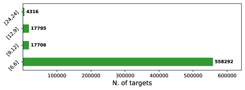
Figure 12: Target distribution over the closest box size priors. The association is made using the Euclidean distance in the 2D size space.

3.7.3 Source properties to predict

With our method, regardless of the application, each detection unit must always predict the box center coordinates ($x,y$), the box size ($w,h$), and one of or both the probability $P$ and the Objectness $O$. For all the remaining parameters requested by the SDC1 task, namely the source flux $f$, the major axis size $Bmaj$, the minor axis size $Bmin$, and the position angle $PA$, we can use the extra-parameter prediction capability of YOLO-CIANNA (Sect. 2.4). As stated in Sect. 3.1, we choose to ignore source classification and the associated core fraction and, therefore, do not predict these properties. Still, the scorer requires values for these parameters to compute the per-source score. We then adopt the simple approach of setting a constant value for these parameters for all sources. We found that setting $cf=0.0375$ and $C=2$ (corresponding to SFG) resulted in the best average sub-scores over the full catalog with $\bar{s}^{cf}=0.9865$ and $\bar{s}^{C}=0.9734$.

For all the extra parameters, their output activation is linear (Fig. 3), and we have to normalize them to be all in a similar range. For the source flux, we apply minimum and maximum clipping limits so $f$ is in the $[1.9{\times}10^{-6},2{\times}10^{-3}]$ Jy range, followed by a log10 rescale. The resulting distribution is then linearly rescaled in the 0 to 1 range using the clipping limits as interval edges. We stress that our target is the apparent flux in Jy, obtained by multiplying the integrated source fluxes from the True catalog by the interpolated primary beam value at the source central coordinates. $Bmaj$ and $Bmin$ follow the same normalization scheme, with $Bmaj$ in the $[0.9,60.0]$ arcsec range and $Bmin$ in the $[0.3,30.0]$ arcsec range. For $PA$, it is very important to consider if the source is resolved or not. Trying to predict the position angle of an unresolved source would result in training noise. We first search for all sources with $Bmaj\leq 1.8$ arcsec and attribute them a target of $\hat{PA}=0$. We note that this filtering only applies when defining the target and that nothing prevents the detector from predicting an angle for smaller sources at prediction time. We then define two predicted parameters, $\cos{(PA)}$ and $\sin{(PA)}$. Considering that the target $PA$ is in the $[-90,90]$ degree range, we linearly rescale $\sin{(PA)}$ to the 0 to 1 range. Due to angular symmetries and degeneracies of PA, predicting both $\cos{(PA)}$ and $\sin{(PA)}$ with the network and then reconstructing the predicted $PA$ to add to the source catalog works better than a direct angle prediction. In summary, each box predicts the following vector for each source $\left<x,y,w,h,P,O,f,Bmaj,Bmin,\cos{(PA)},\sin{(PA)}\right>$. As discussed in Sect. 2.4, we can set independent $\gamma^{p}$ scaling values for all parameters to balance their respective importance in the loss. We list the $\gamma^{p}$ we used for all parameters in Table 3.

3.7.4 Remaining hyper-parameters

We list all the hyper-parameters for our application here for reproducibility purposes, even if some of them are only described in the appendix Appendix A.3, with the advanced description of the association process of YOLO-CIANNA. We use the alternative ${\rm DIoU}$ matching metric, described in Appendix. A.4, which implies that the $L^{{\rm fIoU}}$ limits can take values in the -1 to 1 range. Following our nine detection units definition with 3 scales, we set $\lambda_{void}=0.15$ for the 6 small detection units and $\lambda_{void}=0.01$ for the 3 larger ones. The different $\lambda$ scaling factors, along with the corresponding pre-activation scaling and limit values, are given in Table 2. The various $L^{{\rm fIoU}}$ and some other remaining hyperparameters are given in Table 3. For a more exhaustive view of all the detector hyperparameters, we recommend reading the provided example SDC1 scripts archived with CIANNA V1.0.

Table 2: List of scaling and limits related to the loss sub-parts.

	Pos.	Size	Prob.	Obj.	Param.
$\lambda$	36.0	0.2	0.5	2.0	5.0
Pre-activ. scaling	0.5	0.5	0.2	0.5	0.5
Pre-activ. max	6.0	1.2	6.0	6.0	1.5
Pre-activ. min	-6.0	-1.2	-6.0	- 6.0	-0.2

Table 3: List of some of the detector hyperparameters.

Parameter	$\gamma^{f}$	$\gamma^{Bmaj}$	$\gamma^{Bmin}$	$\gamma^{cos{(PA)}}$	$\gamma^{\sin{(PA)}}$
Value	2.0	2.0	1.0	0.5	0.5
Parameter	$L^{{\rm fIoU}}_{gbnb}$	$L^{{\rm fIoU}}_{low}$	$L^{{\rm fIoU}}_{P\_good}$	$L^{{\rm fIoU}}_{O\_good}$	$L^{{\rm fIoU}}_{p\_good}$
Value	0.5	-0.1	-0.3	-0.3	-0.1
Parameter	$S_{ar}$	$\alpha_{small}$	$N_{rand}$	$\alpha_{best}$	$\alpha_{rand}$
Value	0	0.0	16000	0.90	0.02

3.8 Detector training

The layer weights are initialized to random values following a Glorot normal initialization (Glorot & Bengio, 2010), the batch size is set to $b_{s}=16$, and the numerical resolution is set to full 32-bit floating point for all network elements. Our default learning rate is $1.5{\times}10^{-4}$ with an exponential decay of $5{\times}10^{-4}$ as a function of the training iteration up to a minimum value of $5\%$ of the default learning rate. A constant weight update momentum of 0.8 is also used. No weight decay is used since it always resulted in lower scores. The first 40 iterations are done using an increasing learning rate up to the reference value, and the initial random association is set to $N_{rand}=16000$ (Appendix A.6.2).

With our fully convolutional architecture, we could technically use any input size that is a multiple of the network reduction factor (see Appendix A.1). A too-small input size can cause many cutout edge effects, and a too-large input size reduces the number of examples that can be constructed from a finite training area, increasing the chances of overtraining. For our specific application, we observed that a training input size of $256{\times}256$ pixels resulted in the best achievable score. During training, we dynamically generate groups of 1600 augmented images that we refer to as a training iteration. For each example, we draw a random pixel position inside the training area, extract a small region corresponding to our network input size, and apply multiple pixel-preserving operations randomly from vertical or horizontal flips and $90$ or $-90$ degree rotations. Due to how astronomical images are constructed, any transformation that resamples the pixels must be avoided. Images from the additional noise region are selected at a low $5\%$ rate and follow the same augmentation rules. By cutting out patches of the larger image, sources on the edges of a patch might be cut, which can have a strong negative impact on the detector capabilities (see Sect. 3.4). We tried various approaches for handling these sources (Appendix A.6.4) but obtained the best scores with a simple exclusion of any target box that is not fully contained in the cutout.

Because the labeled area is small, we need to preserve all of it in our training sample. Our validation dataset is then defined from the same region and catalog but using a fixed grid of non-overlapping patches for a total of 100 images. We acknowledge that this is non-optimal as it would fail to identify overtraining. However, we can rely on the SDC1 scorer to provide an independent metric on a separate dataset to evaluate our detector performances at a regular iteration interval. We also use the score over the full image field to optimize the individual objectness limits for all detection units from a trained network. We emphasize that this optimization is a simple refinement and that we would still achieve more than $95\%$ of our best score with naive guesses on these values instead of searching for the best ones.

With this setup, the detector reaches a high score after only 400 iterations, but the larger sources are not properly constrained, and the global characterization is sub-optimal. The detector usually requires around 3000 iterations to converge. After that, it oscillates for a few hundred iterations and eventually exhibits overtraining, lowering the score by up to $5\%$. We present the validation loss with scoring stamps every 200 iterations in Fig. 13. We note that using stricter values for parameters that control the association process like $L^{{\rm fIoU}}_{gbnb}$ or $L^{{\rm fIoU}}_{low}$ would speed up the training. It would result in more stable results, but it usually decreases the best achievable score by a small amount.

On an RTX 4090 GPU and by doing image augmentation on the CPU in parallel, we can reach almost 400 images per second of training performances. Reaching iteration 3000 takes around 3.5 hours. With the current training setup, the GPU memory footprint of the network is around 8GB. A save file representing the model at a given iteration requires 50MB of storage. We tried using different types of mixed-precision along with Nvidia AI-dedicated tensor-cores acceleration for training, but it always resulted in a decrease in score of about $2\%$. Still, it speeds up network training compute performance by a factor of up to $1.8$ while preserving the relative performance impact of various hyperparameters, allowing a more efficient exploration of network architectures and hyperparameter combinations.

3.9 Prediction pipeline

Table 4: First NMS rejection limit pairs.

$L^{{\rm fIoU}}_{NMS}$	0.05	-0.1	-0.3	-0.5
$L^{Obj}_{NMS}$	1.0	0.7	0.5	0.3

To use our trained detector on the full SDC1 image, we need to decompose it into patches. As before, due to the fully convolutional structure of our detector and its resolution static prediction (Appendix A.1), we can technically use any input size for prediction. As for training, decomposing the image into patches results in sources being close to the edges of a patch, which are then poorly detected or characterized. To overcome this at prediction time, we use overlapping patches with an overlap size of 32 pixels, corresponding to the size of two grid cells and half our maximum clipping size for our target boxes. Each source is then more likely to be well represented by at least one patch. In case of multiple detections of the same source by two patches, the objectness score can be used to select the best one through an inter-patch NMS process. From there, we observed that larger patches tend to produce better results as they reduce the proportion of sources close to an edge. We settled for a prediction input size of $512{\times}512$ pixels, which results in a good balance between prediction quality and compute efficiency. By setting a small offset on the edges of the full image, we can obtain a map made of $67{\times}67$ partially overlapping patches.

For each of them, we first apply a per-detection-unit objectness threshold filtering. The threshold values are obtained through score optimization by identifying the objectness interval contributing positively to the score (Sect. 3.3 and Eq. 22). We also add a rejection criterion based on the average pixel flux value in the box area as a function of the predicted objectness score to exclude many small false detections induced by very large and bright sources. Multiple detections are then filtered by the NMS process for each patch (Sect. 2.8), using multiple $L^{{\rm fIoU}}_{NMS}$ and $L^{Obj}_{NMS}$ thresholds pairs that are given in Table 4. Following the NMS process, considering the best current score box, any other box that respects one of the condition pairs ${\rm DIoU}>L^{{\rm fIoU}}_{NMS}$ and $O<L^{Obj}_{NMS}$ is removed. With this setup, the rejection chance is based on a combination of the detection confidence and the distance to other confident detection. To filter multiple detections from overlapping patches, we use a secondary inter-patch NMS process. It works exactly as the first NMS but with a constant $L^{{\rm fIoU}}_{NMS}=-0.15$. From the filtered box list, we can construct a catalog in the scorer format by inverting our normalizations on the predicted parameters and also convert the predicted apparent flux back to a real flux using the interpolated primary beam value at the position of the detection.

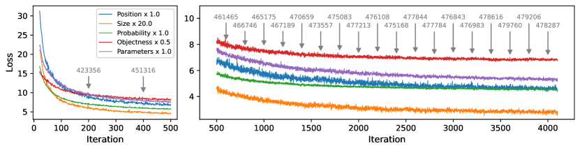
Figure 13: Evolution of the validation loss sub-parts during training, using the ”natural” loss representation (Appendix A.7). The first 20 iterations are skipped. Optimized scores obtained using the procedure described in Sect. 3.9 are displayed every 200 iterations (one or two points differences can be observed compared to Table 5 due to rounding of the objectness thresholds).

On an RTX 4090 GPU, the raw prediction compute performance at the largest available batch size is around 300 images per second for an input size of $512{\times}512$ pixels, or almost 80 million pixels per second. The raw processing time for the full 4GB image of 32768 square pixels after the network loading is around 15 seconds. To this, we need to add the post-processing time of the prediction pipeline, which strongly depends on the minimum objectness threshold values for the different detection units. With an end-to-end Python processing pipeline that only produces the converted detection catalog, this processing time can be reduced to approximately 40s on a single CPU core (Ryzen 9 5900X). Interestingly, the detection performances are fully preserved when doing the prediction in mixed-precision using 16-bit numerical computations with a 32-bit accumulator when necessary, allowing the use of Nvidia AI-dedicated tensor-cores compute units available on modern GPU architectures. With this, we can reach around 500 images of size $512{\times}512$ per second, or around 130 million pixels per second, of raw computing performance. At this point, saving the results on our local high-end SSD storage becomes the limiting factor, and the network loading time becomes comparable to the prediction time over the full image. This confirms that our method is perfectly suited for very large surveys and real-time source detection (Sect. 5.3).

4 Results and Analysis

In this section, we present the results of our best training setup over the full field of the selected SDC1 image. We stress that there are small variations of results from retraining a network using the same training setup, with typical variations of the best achievable score around $\pm 0.5\%$. In practice, the detailed analyses carried out on this specific training hold perfectly with any training using the same setup. The results in this section are ordered following the post-processing pipeline from the raw predicted quantities up to the predicted source catalog using the challenge format. The validation loss curve as a function of the training iteration is presented in Fig. 13. This figure also indicates the optimized score at a regular interval of 200 iterations. The following results are presented for iteration 3600, which achieved the best score for this specific training.

4.1 Patch-divided prediction results

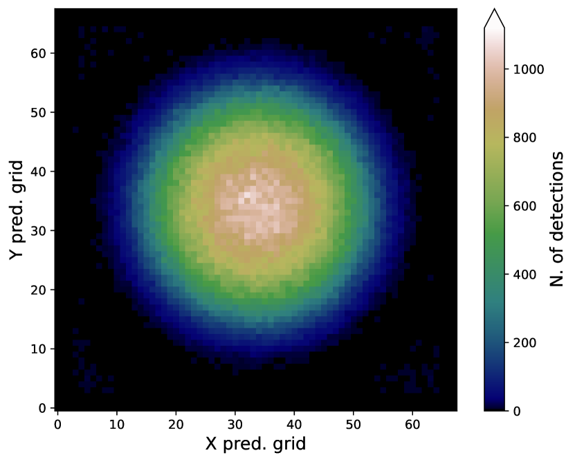
Figure 14: 2D representation of the full SDC1 image field decomposed into overlapping patches. Each pixel corresponds to a specific patch, and the color represents the number of detected sources after objectness filtering and in-patch NMS. The central coordinates of the field are $\textrm{RA}=0$ deg, $\textrm{Dec}=-30$ deg.

From the raw model prediction, after applying the first objectness filtering and the in-patch NMS, we can obtain a list of all the detected sources per patch. We represent the respective number of sources for all patches over the full image field in Fig. 14. We note that some sources are counted multiple times in this representation because the inter-patch NMS has not yet been applied. We see that the detector sensitivity follows the primary beam imprints over the full image. We do not observe a clear overdensity of detected sources in the training area region, which would be a clear sign of overtraining.

To analyze in detail the behavior of the individual detection units from our detector output (Sect. 2.5), we represent a histogram of the number of found-useful detections per grid cell for all patches in Fig. 15. Here, empty grid cells are excluded, but they represent the more common case, especially considering that we keep patches far from the image center. We observe that cases with 6 or more detections are very few, 4 or 5 detections are not common but significant, and most non-empty grid cells contain less than 3 detections. Further analysis indicates that only around $26\%$ of the non-empty grid cells have more than 1 detection, and this proportion drops to $4.5\%$ for more than 2 detections. In fact, the in-patch NMS process removes $78\%$ of the raw good detections. This indicates that many detection units are in use and capable of detecting real sources, but they often end up detecting the same sources. Still, we observed that lowering the number of detection units lowers the score, indicating that they are useful for some specific contexts or that having more detection units better distributes the information. To further verify this idea, we represent in Fig. 16 a histogram of the number of predictions per detection unit for the whole image. The distribution over the different detection units from the small-size regime is relatively homogeneous, confirming that all detection units are useful. We also observe that the relative proportions of each size regime are well preserved regarding the theoretical target distribution from Fig. 12, which confirms that our association process properly distributes the information over the available size regimes.

To have a better view of the representation regime of individual detection units, we can look at their respective distribution of predicted sizes and aspect ratios in Fig. 17. We observe that some boxes are more specialized regarding aspect ratios, which is natural for the intermediate size regime due to the two different ratios of size priors. The behavior of the small-size regime detection units is more surprising, as it appears to prefer a positive aspect ratio for small but resolved sources. The cause of this behavior remains unidentified, but we can firmly state that it does not come from the training sample for which the target box aspect ratios are well balanced. Finally, the detection unit from the large-size regime and usually one or two from the small-size regime predict boxes with actual sizes that would be more representative of the intermediate regime. Due to the significant difference in aspect ratio, only one of the intermediate-size regime detection units is likely to be used in a given grid cell. In cases where two or more sources of intermediate size have to be detected in the same grid cell, a small or large box with a square prior might be preferable to using the wrong aspect ratio box of the appropriate size regime. This effect is less visible if we train our detector using only square priors.

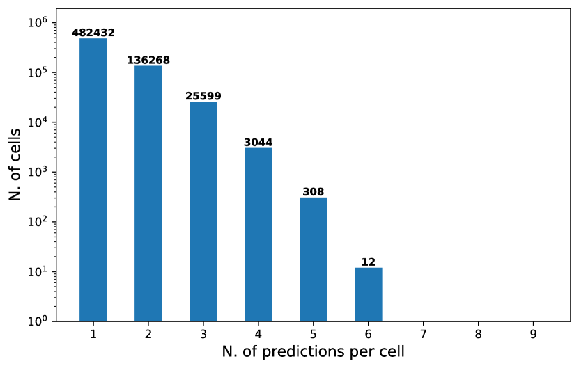
Figure 15: Distribution of the non-empty grid cells regarding the number of detections in each cell, after objectness filtering and in-patch NMS.

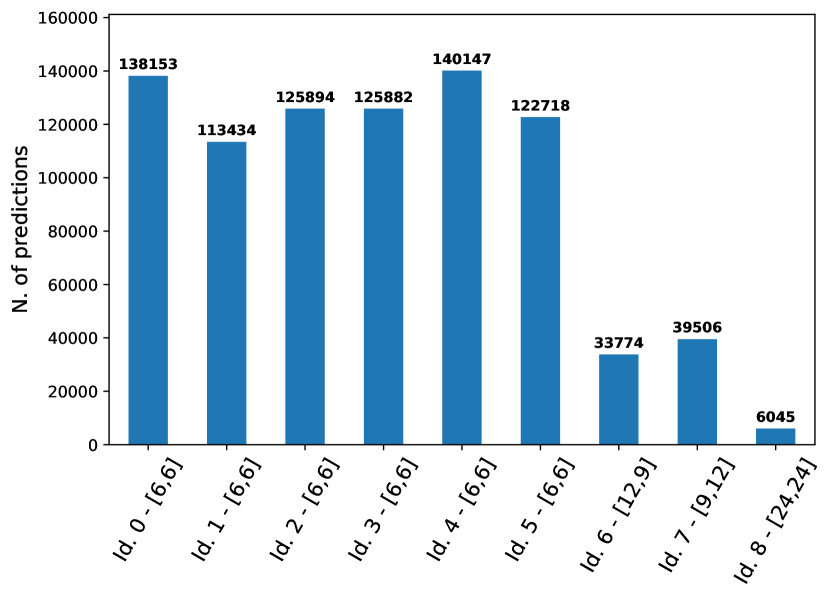
Figure 16: Distribution of the detections regarding the detection unit that produced them, after objectness filtering and in-patch NMS. The size prior is indicated for each detection unit.

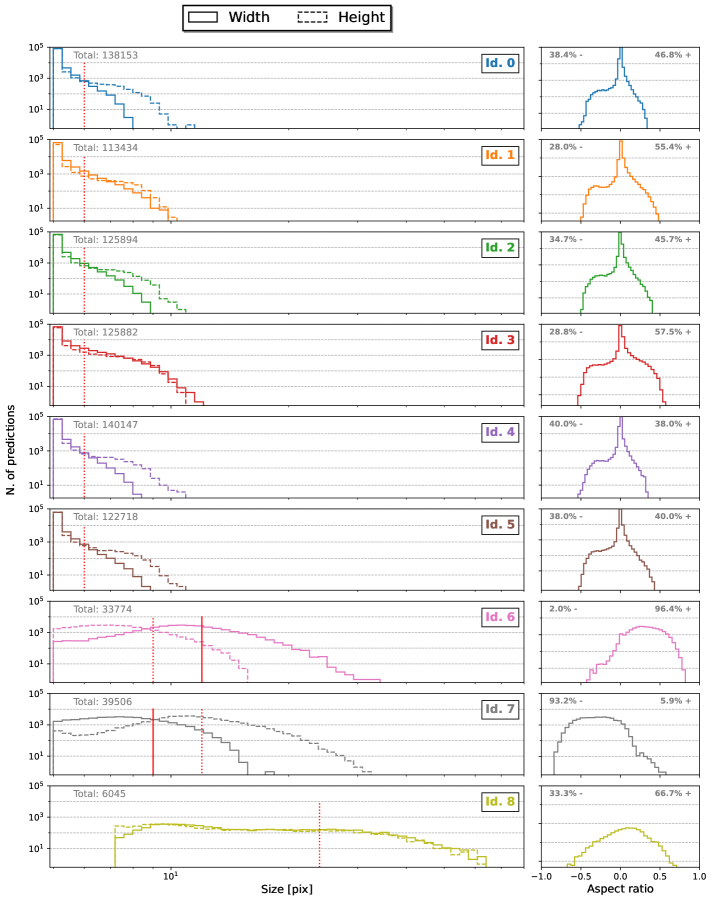
Figure 17: Histograms of the predicted heights, widths, and aspect ratios for every detection unit. The aspect ratio is computed as $(w-h)/\max{(w,h)}$. The total number of predictions and the proportion of strictly positive and negative aspect ratios are also given for each detection unit. The red vertical lines indicate the width and height of the size priors.

4.2 Full catalog scoring

Table 5: . List of SDC1 scores and related properties for source catalogs from different teams and methods.

Team (method)	$M_{s}$ (Score)	$N_{det}$	$N_{match}$	$N_{false}$	$N_{bad}\in N_{false}$	Purity	$\bar{s}$
Post-challenge results
MINERVA (YOLO-CIANNA-ref)	479758	718760	677025	41735	15787	94.19%	0.7703
MINERVA (YOLO-CIANNA-alt)	414937	538649	533659	4990	2402	99.07%	0.7869
JLRAT2 (JSFM2)	298201	502146	484212	17934	2274	96.43%	0.6529
Original challenge results
Engage-SKA (PROFOUND)	200939	421992	418384	3608	2677	99.15%	0.4889
Shanghai (multiple methods)	158841	292646	291553	1093	698	99.63%	0.5486
ICRAR (CLARAN)	142784	279898	259806	20092	6875	92.82%	0.6269
…	…	…	…	…	…	…	…

Note. The bold element represents the target metric that is optimized for each result.

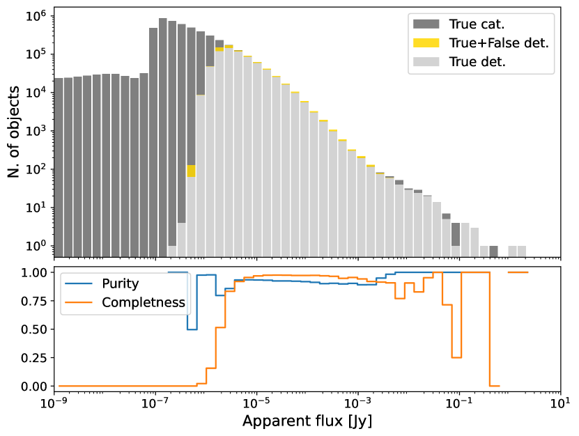
YOLO-CIANNA-ref

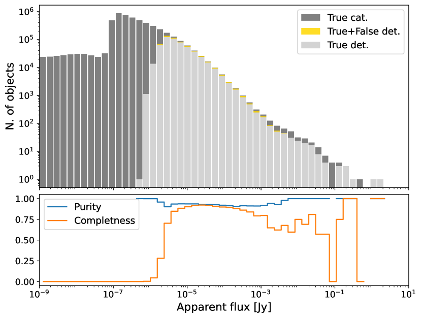
YOLO-CIANNA-alt

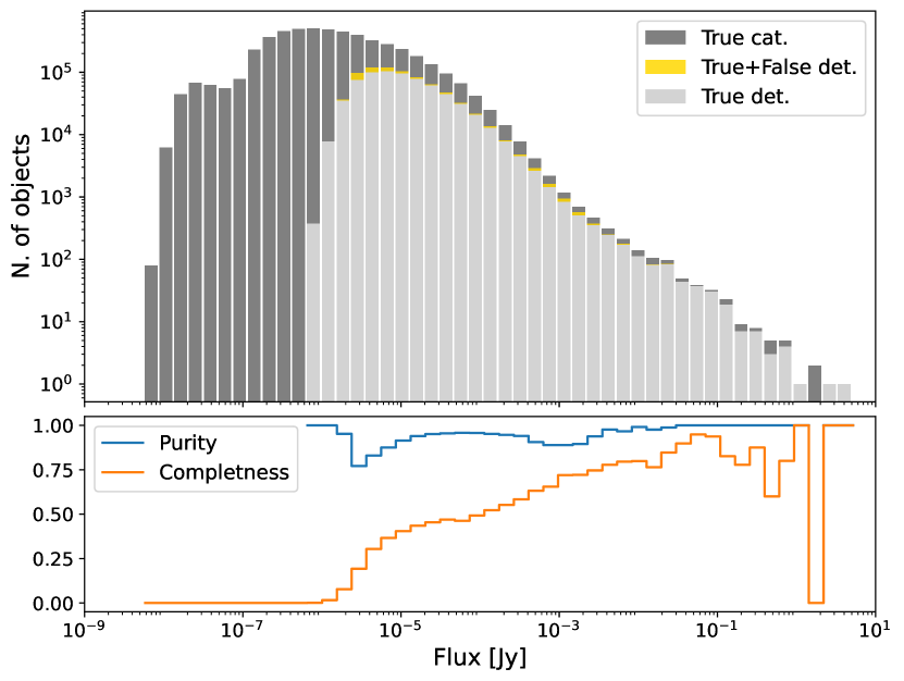
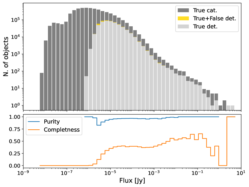
Figure 18: Histograms of the sources as a function of their flux using logarithmic bins for the underlying True catalog and the predicted sources in the testing area. The true source flux is used for matches, while the predicted flux is used for false positives. The bottom part of each frame represents the purity and completeness of each bin of the histograms (defined in Sect. 4.2). The top frames use the apparent flux after multiplication with the primary beam, while the bottom frames use the integrated flux. The left column represents the results for the YOLO-CIANNA-ref model, and the right column the YOLO-CIANNA-alt model.

After the inter-patch NMS filtering and conversion of all the predicted source parameters, we obtain a source catalog for the full image that can be put through the SDC1 scorer (Sect. 3.3). It automatically excludes the training area from both the submitted and True source catalogs and produces a detection score for the rest of the image. Our reference score for this model is presented in Table. 5 under the name YOLO-CIANNA-ref, along with other scores from the top three originally participating teams on the same single 560 MHz - 1000h image. The Engage-SKA team used the ProFound package (Robotham et al., 2018), which is a collection of astronomical image processing and analysis tools that produce segmentation maps. The Shanghai team worked with a combination of three classical astronomical source-detector packages, namely AEGEAN (Hancock et al., 2018), DUCHAMP (Whiting, 2012), and SExtractor (Bertin & Arnouts, 1996), but ended up using only the last one to construct its catalog. Finally, the ICRAR team used a deep learning approach with the CLARAN method (Wu et al., 2019), with a region-based method similar to R-CNN (Girshick et al., 2013). We note the participation of another team that used a very shallow convolutional network structure for segmentation, achieving a much lower score with the ConvoSource method (Lukic et al., 2019). We also include another post-challenge score from Yu et al. (2022), which is a refinement of the JLRAT team that participated in the original challenge but with a lower submitted score, also with a deep learning-based method using a combination of a region-based approach with a feature pyramid network. Their new catalog is publicly available and is provided in the scorer format, allowing us to include their result on the same image in the table. Our reference score catalog is also made publicly available with the present paper so the full table can be reproduced. In addition to the challenge score, we also indicate the number of sources retrieved, the precision of the submitted catalog, and the average source characterization score.

The source catalog obtained with our YOLO-CIANNA detector improves the best-submitted score of the originally participating teams by +139% and the score of the only other published post-challenge score by +61%, which already significantly outperformed what was submitted during the challenge. We observe that the teams that competed in the challenge and obtained good scores are the ones that focused on catalog purity. This is likely to be due to their relatively low average source characterization score, which is discussed in Sect. 4.4. As the apparent flux should be an appropriate first-order proxy to represent the detection difficulty, we present the apparent flux distribution of our detections in comparison to the True catalog in Fig. 18. We also present the completeness and purity of our catalog for each flux bin. The completeness represents the proportion of total sources we successfully detected, and the purity represents the proportion of the proposed detection that are real sources. These quantities are computed based on the full True catalog and SDC1 matching criteria. Comparing this flux distribution with the one from our selected training sample (Fig. 8), we observe that our detector can identify sources outside its training flux range close to the noise limit. This is likely to correspond to sources for which the perceived apparent flux was increased by the local noise or blended faint sources that add their flux so the network detects them as a single brighter source (Sect. 3.4). These two cases will result in sources with a target apparent flux close to or below the detection limit to be detected. This out-of-range detection capability is clearly visible in the example fields from Fig. 20. We also see that the completeness is high in the intermediate apparent flux range but drops progressively at lower flux values. While it can be explained by sources getting under the detection noise limits, it can also come from sources too blended to be detected individually. In such a context, the prediction will be associated with the brightest target, removing mostly low apparent flux sources. These missed sources are also visible in the example fields from Fig. 20. On the other side of the flux range, our detector does not recover a few bright sources, which can be explained by the absence of similar examples in our training sample. While they are too few to influence the scoring by their absence, they can still have a strong effect by adding false positives, which is discussed in Sects. 3.9 and 4.1.

4.3 Alternative purity focused detection

By trying to optimize for the best possible SDC1 score, we are forced toward a predefined catalog purity. In fact, our per-source characterization score defines the ratio of true-to-false detection above which the detections add score points (Sect. 3.3). This relation is not linear, as objects that are difficult to detect will likely be difficult to characterize. This is why we optimize the score using the ordered detection in objectness, which reflects the network confidence (Sect. 3.9). If catalog purity is the main concern, we can adjust the objectness threshold selection to select more confident detections without retraining the detector. With this approach, we can evaluate the performance of a given trained detector in different confidence regimes. We define the YOLO-CIANNA-alt catalog, obtained by searching for objectness thresholds that enforce a 99% purity on the same network. The corresponding score is presented in Table. 5. This purity-focused catalog produces a score that is 13% lower than our reference result but still much higher than other submissions. We observe that the average source score also increases with this selection, which confirms that the predicted objectness captures information about both the detection and characterization difficulty of the sources.

We represent the apparent flux distribution of this purity focus catalog in Fig. 18. Comparing this distribution with our reference result shows that the detections at low and high apparent fluxes get removed first. While the link between low flux and difficulty is straightforward, it is less clear why bright objects get removed more than intermediate apparent flux regimes. Our interpretation would be that the small number of bright source examples in the training sample leads to poor characterization, resulting in lower detection confidence. By looking at the distribution of false positives over the full image, we observe a much more homogeneous distribution than with the YOLO-CIANNA-ref model. Therefore, the optimized set of objectness thresholds for the purity-focused model seems to be driven by regions of the image that are in the intermediate beam regime that is interpolated between our training regions.

As discussed in Sect. 2.2, having a confidence score that is mapped by a continuous function means that the network samples all its sensitivity regimes simultaneously. From a user perspective, a given trained model can be adapted to various applications with either completeness or purity requirements. We discuss how this principle could be used to design an alternative detection metric in Sect. 5.2.

4.4 Source characterization

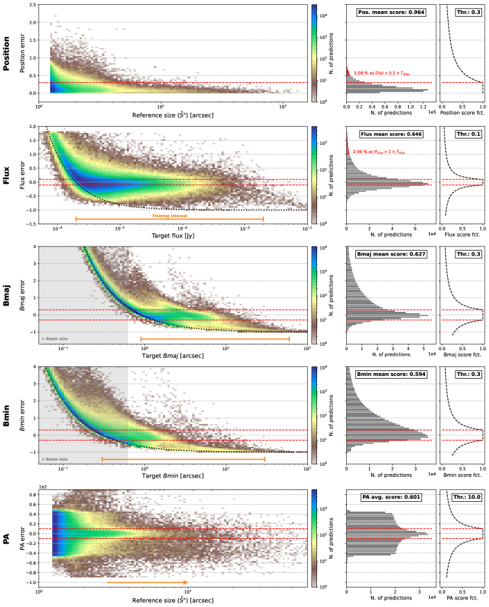
Figure 19: 2D histograms of the different parameter errors defined by the scorer as a function of relevant difficulty proxies. The left column represents the 2D histograms. The right column represents a 1D histogram of the relative error projected over the same axis as the left column. To the right of this projection and using the same axis projection, we indicate the specific response of the score function for each parameter following Eq. 19 and Fig. 6. The red dashed line indicates the edges of the area for which the parameter score is saturated at its maximum value. The orange lines and arrow indicate the reference values that are represented by the training sample. The gray overlay represents the area of the distribution for sources that are smaller than the beam size.

In addition to the global score, the scorer code can be configured to produce detailed results, including the list of sources that are considered a match, along with the predicted and target properties for each of them. In the following sections, we use these products to perform a detailed analysis of the characterization capabilities of our YOLO-CIANNA detector.

A primordial aspect of our produced source catalog is its high source characterization performance with $\bar{s}=0.7703$. Before analyzing it in detail, it is important to highlight that parameter prediction accuracy is impossible to decorelate from the detection capability. The average parameter score ignores the fact that the characterization is not equally difficult for all sources. For example, we could choose to detect the 10 sources that are the easiest to characterize and obtain a very high characterization score. In contrast, a method that detects many sources, including some that are difficult to characterize, would obtain a lower average characterization score even if it is better at characterizing the specific 10 easiest sources. This effect is well illustrated by the increase in average source score for our alternative purity-focused results compared to our reference score result in Table 5. Overall, this average source score metric penalizes more efficient source detectors that properly detect more difficult sources. To overcome this limitation, it would be possible to order or bin the sources by difficulty before evaluating the characterization capability of different methods on each bin. However, it seems impossible to define a characterization or detection difficulty proxy that would be method agnostic. The best yet incomplete proxies we have are source brightness or signal-to-noise ratio (SNR) measurements. A better solution to compare method characterization capabilities would be to use subsets of sources that are detected by the different methods. In our opinion, this is a significant limitation of the analysis from both SDC1 and SDC2 summary papers.

Our approach to overcome this difficulty is to use 2D histograms of the parameter errors from sources considered as matches by the scorer as a function of a difficulty proxy, which is presented in Fig. 19. This figure also comprises histograms of the sources regarding only the parameter errors, which are directly aligned with their respective score response functions to ease the comparison. The following sub-sections detail the prediction capability for each type of predicted parameter.

We achieve a very high positioning score of $\bar{s}^{pos}=0.964$, which is, in fact, a requirement for reaching a high detection recall and precision regarding the scorer match criteria. For point sources to be considered a match, we must reach sub-pixel positioning accuracy (Sect. 3.3). This typically explains why we configured our detector with a strong focus on the position loss in Table 2. From this point of view, the 0.3 error threshold for the position seems quite permissive and is not very useful in comparing methods regarding their positioning accuracy.

Regarding the flux prediction, the distribution mostly centers on the score function response, granting a good average flux score of $\bar{s}^{flux}=0.646$. As for the position, sources with a bad flux prediction are more likely to be rejected based on the scorer match condition (Sect. 3.3), imposing practical limits on the accessible flux dispersion. For faint sources, the detector overestimates the flux, which is typical of regression prediction when generalizing below the training range limit. Overall, the detector tends to predict the minimum flux value it was trained on for any fainter objects. Still, we note that the faintest sources are only detectable when the local noise increases their apparent flux. This can result in a selection effect that is likely to bias the network training to overestimate the underlying flux of faint sources. This can explain the spreading of the flux predictions above the minimum training value prediction. For the few bright sources, we see that our detector underestimates the predicted flux, which is induced by our maximum value at training time. We also note that the pixel cut limits combined with the dynamic rescale we applied to our input image could contribute to these flux prediction limits (Sect. 3.7.1). Still, trying other normalization cuts did not result in significant flux prediction improvements.

Regarding $Bmaj$ and $Bmin$, the global predictions are convincing and centered on the score response function with $\bar{s}^{Bmaj}=0.627$ and $\bar{s}^{Bmin}=0.594$, but we observe the same type of out-limit generalization behaviors. Here, these effects are reinforced by the fact that the True values to be predicted are not convolved with the synthesized beam. In practice, the detector is expected to predict non-available information for most point sources that are actually detectable. Still, we observe that predictions for $Bmin$ are surprisingly not completely collapsed toward a single solution below the synthesized beam size. In practice, we have adjusted our clipping values to reflect this capability that was observed during our first testing, so it is now at the best limit we could reach. For $Bmaj$ specifically, we observe that the predictions are distributed over two independent prediction regimes that both follow the same type of error function. This separation is induced by the source distribution over different detection units based on their size. This creates a discontinuity as only detection units with a large size prior are properly constrained to predict large $Bmaj$ values, while it is the opposite for detection units with small size priors. We note that this effect is strongly mitigated by the addition of the random box association regularization in our association function (Appendix A.6 and Fig. 4) that forces detection units to generalize outside of their size range. By forcing more detection unit independence, the different size regimes get more separated in the figure.

For the position angle, the average score is surprisingly high with $\bar{s}^{PA}=0.601$, considering that most detected sources are smaller than the beam resolution limit. From the distribution, we observe that the prediction is not too noisy and that small sources distribute evenly over the error range, while the prediction accuracy improves progressively with the increase in source size.

4.5 Example fields

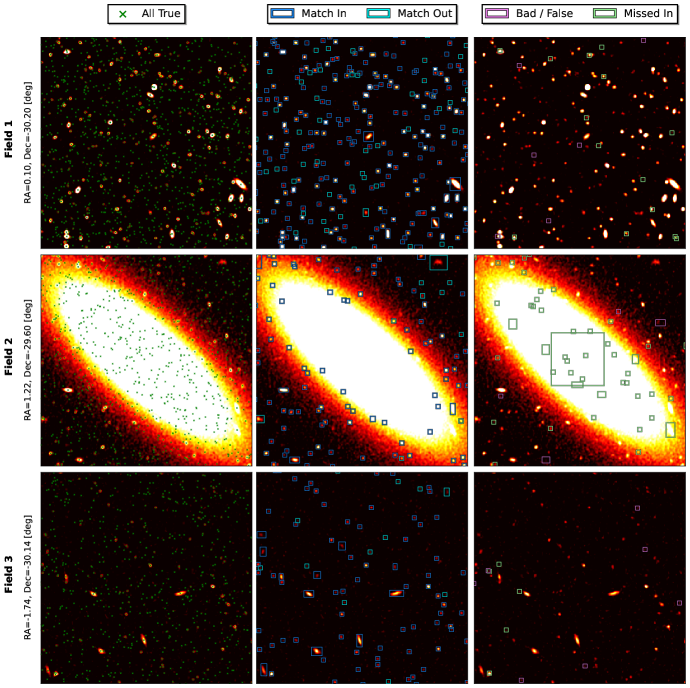
Figure 20: Distribution of sources and predictions for three 256 square pixels example fields. The background images use the same clipping and normalization as the network input (Sect. 3.7.1) but are saturated at $50\%$ of the maximum. Each line represents a different field. Left: scatter plot of the central source coordinates from the full True catalog. Middle: boxes for predictions that match a true source based on the scorer. The match-out boxes indicate properly detected sources with a target flux below the minimum value in the training sample, so outside our selection function criteria (discussed in Sect. 4.2). Right: boxes for true sources that pass our selection function but are not detected, and boxes for predictions that are false positives based on the scorer.

We illustrate the detected boxes from our reference model over a few example fields from the SDC1 image outside the training area in Fig. 20. We use the same field size as our training input window, namely $256{\times}256$ pixels. The first field represents the central region where our detector reaches peak detection performance. This field illustrates the capability of our detector to identify faint sources outside of its training interval (Sect. 4.2). A few sources are considered missed, but almost all of them are blended with sources that are already properly detected. The few false detections can be separated into three cases: i) it is near a properly detected source, but our NMS process did not remove it, ii) it is near a source, but the matching criterion failed, certainly due to the target flux being lower than the minimum accessible flux, or iii) it is near a compact signal that does not correspond to a source. The first and second cases are the most common.

The second field illustrates the extreme case of a large resolved galaxy. As previously stated, there is no similar source in the training area that the network could have learned to identify. Therefore, missing the large source itself was expected. However, this field illustrates our detector capability to prevent false detections in such a context. There are only a few detections considered to be false, and most of them seem to represent a real underlying source, indicating that the matching criteria likely rejected it because of the predicted flux or size. Several blended sources are also properly detected on the edges of the large source. We purposely saturated all the images at the lower half of the input dynamic to improve the readability of the figure for faint sources. This explains why the detector manages to identify blended sources in bright regions that appear saturated. There are many missed sources in this context, which are just completely hidden by the bright source and, therefore, undetectable.

The last field illustrates a region far from the image center but still in a primary beam regime where several sources can be detected. This is typical of the intermediate regime between the default training area and our noise-only areas. With this field, we can verify the capability of our detector to interpolate between the two training contexts. While most sources are properly detected, we observe that the number of false positives is slightly higher than in the first field while still preserving a relatively high purity. There are only a few considered missed, and their origin is likely the same as in the two other fields. This field is typical of the regions of the full field for which we identify an overdensity of false detection in Fig 21.

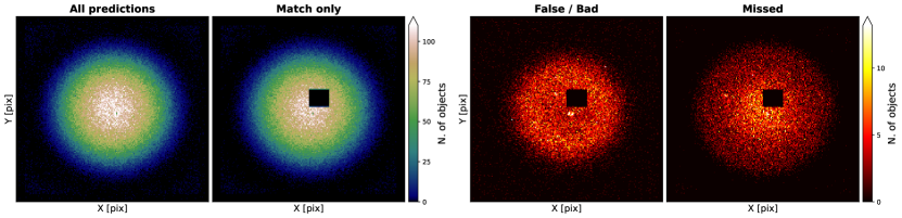
Figure 21: Distribution of various kinds of ”objects” over the full SDC1 field, minus the training area when necessary, for the YOLO-CIANNA-ref model. The match and false detections are based on the scorer, while the missed ones are based on our selection function. This figure represents absolute numbers of detections and not relative ones, so the distribution is relevant, but the actual value is scaled by the total number of detections. The central coordinates of the field are RA=0 deg, Dec=-30 deg.

4.6 Full field distribution

Using the match criterion from the scorer, we can look at the match distribution over the full field and the distribution of false positives and missed sources, which are all illustrated in Fig. 21. As expected, all distributions follow the primary beam imprint over the field. The striking feature of this figure is that the false positives seem more concentrated in a ring that spans from the farthest point of the training area up to the edge of the primary beam. This is a direct consequence of the training area definition, and this specific distribution is more pronounced when we do not include the two additional noise-only regions in our training sample (Sect. 3.5). The distribution of missed sources based on our selection function mostly follows the primary beam footprint, illustrating that our detector completeness is mostly uniform over the full field. Both the distribution of false and missed exhibit compact over-densities of a few pixels, corresponding to the position of the few very large and bright sources.

5 Discussion

5.1 Challenge definition and scorer biases

The SDC1 successfully gathered research teams to adapt, develop, and evaluate detection methods on a controlled dataset with a fixed evaluation metric. Even now that the challenge itself has ended, it remains a very valuable dataset in its challenge form and even more valuable with the added information about the full True catalog. However, as we stated in Sect. 3.2, the use of 4GB images does not really prepare the community for handling data-intensive workloads. The SDC2 and SDC3 editions are more challenging in this regard. In addition, our study highlighted a few limitations that are the result of some design choices of the challenge. In this section, we discuss these specific aspects and also propose a few directions that could help the design of future challenges.

5.1.1 Training area

In Bonaldi et al. (2021), the authors highlight that the source classification aspect is made challenging due to the small number of detectable sources for which all the frequencies are available and the strong class imbalance. As the frequency increases, the size of the training area is also reduced, leading to a very small training sample for supervised learning methods. More generally, they do not illustrate or discuss the distribution of the true sources and false positives over the full image field to highlight the potential effects of the training area selection. We have extensively discussed how having only access to a central part of the image for training affects the generalization capability of our detector Sect. 3.5 and proposed a workaround by adding the two extra noise-only training regions. In Appendix. C, we explore an alternative training region that spans over a full field radius to encapsulate all the sensitivity regimes from the primary beam. We demonstrate that this simple change solved most of the related issues. Overall, the SDC1 falls in a classical definition hiccup regarding supervised learning approaches, that is, having a training sample that does not represent the final task to perform. Interestingly, this aspect was corrected for the SDC2 (Hartley et al., 2023) by providing the training example in the form of an independent data cube, which is another statistical realization of the same underlying simulation.

5.1.2 True catalog properties

We discussed in Sect. 3.4 how much the construction of the training sample matters, especially regarding the selection of detectable sources only. While sampling the transition between detectable and non-detectable sources with a sufficient margin is a good thing, keeping the vast majority of nondetectable objects in the reference True catalog can cause several issues. At testing time, it strongly increases the chance of random association. To counterbalance this effect, strong matching criteria have been used in the SDC1 scorer, which then causes the rejection of properly detected sources too often. We note that in Bonaldi et al. (2021), the authors indicate that background faint sources contribute to the realism of the image noise. Still, most of them could have been ignored during scoring to reduce the random matches over undetectable sources. In all cases, a selection function must be defined to select a specific point in the detectable to undetectable transition. In this regard, the provided True catalog could have contained more information directly from the simulation instead of just the source properties to predict. This would have allowed the construction of a more advanced selection function while not changing the amount of information in the image from which the detection has to be made.

Some other design choices do not directly impact the detector performances but could have been made differently to serve other purposes. For example, the True catalog contains the absolute real values for each source. An alternative approach would have been to provide a single noised realization for each target parameter and accompany them with uncertainty measurements. It would have improved the realism of the reference catalog, considering how target sources can be acquired from real observations, and it would have been possible to add uncertainty predictions to the task by including it in the scorer.

5.1.3 Scorer metric

The main impactful choices are naturally in the evaluation metric itself in the form of the scorer (Sect. 3.3). Firstly, several error thresholds are permissive. Consequently, multiple detection methods with different characterization capabilities will have similar scores for the corresponding source parameters. Secondly, several parameters use an asymmetrical relative error with a symmetrical score response function. This implies that underestimated predictions tend to achieve better scores. Finally, several error functions do not consider the structural limits of the predicted parameters, like resolution limits, which affect, for example, the $Bmaj$, $Bmin$, and $PA$ parameters. Reaching a minimum observational limit for a parameter while the target can be smaller results in a strong positive relative error that is more penalized. This is striking for the Flux, $Bmaj$, and $Bmin$ error distribution illustrated in Fig. 19. Because the score added by a properly detected source depends on its characterization score, successfully detecting difficult sources is poorly rewarded compared to detecting obvious ones. As we discussed in Sect. 4.4, since characterization scores are averaged over all the detected sources regardless of their intrinsic difficulty, a good detector with a good characterization capability will have a lower characterization score than a less complete detector with poor characterization capability. In this regard, one appropriate approach for comparing two method characterization capabilities would be to use subsets of sources identified by the two detectors. In this regard, we strongly encourage any future method application to the SDC1 dataset to include figures that represent the distributed parameter errors as a way to evaluate their characterization capability (e.g., Fig. 19).

To maximize its score, a detector has to identify a maximum number of objects while preserving a given purity dictated by its average source characterization score. However, due to how the scorer was tuned, the accessible score range is quite narrow and does not change much with the actual characterization quality. It means that this challenge is, in fact, strongly detection-focused because an additional identified source always contributes a similar score while a false positive always contributes -1. It is equivalent to having set a fixed purity requirement and tasked teams to compete to achieve the best completion at this purity level. Still, the set of match criteria includes predicted characteristics like the flux and the size of the source. However, to prevent random association with the many non-detectable objects, the detection thresholds on these parameters have been set to strict values. As for the source characterization, the match criterion uses asymmetrical relative errors on quantities with instrumental limitations. When defining a match, the effect of the synthesized beam on the size and position has been accounted for, but nothing was done regarding the predicted flux. Consequently, sources that are perfectly detected regarding the instrument limits can still be considered false positives if their True catalog flux is slightly overestimated due to the relative error asymmetry. In addition, since these sources get lower characterization scores, the detection purity in this regime has to be higher to add a positive score, biasing the detector to remove them more than necessary. This results in underestimating the capability of very strong detectors in low SNR regimes, for which it would be very interesting to compare the various method capabilities.

Another drawback of this scoring approach is that it expects a list of considered true detections, which does not exploit the capability of some methods to order all their detections by confidence. In classical computer vision challenges, they request a per-detection score that is sorted to construct a completeness-purity curve based on a match criterion. The integral of this curve is then used to evaluate the detector capability over its full sensitivity range. We provide more details on constructing the classical mean average precision (mAP) metric in Appendix. A.8.2. Interestingly, since the SDC1 scorer represents a matching criterion, it can be used to construct an AP metric. The match information can then be used to sample the completeness-purity curve. We present the raw and smoothed completeness-purity curve for our YOLO-CIANNA-ref model in Fig. 22, along with the binned purity as a function of the objectness for each detection unit. Since most of the objects in the simulation are non-detectable, the resulting AP is low, but it should remain sensitive to variations in detection capability. As a reference, we achieve ${\rm AP_{SDC1}}=14.3428\%$. While this is an interesting alternative detection metric, it does not account for the source characterization of the detected sources, except as a part of the match criteria.

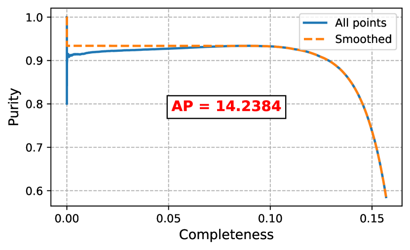
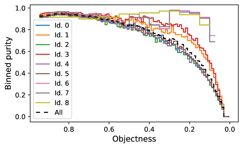
Figure 22: Detector sensitivity curves for the YOLO-CIANNA-ref model. The top frame represents the raw and smoothed purity-completeness curve on which the AP is computed. The bottom frame represents the binned purity as a function of the objectness for all detection units. The bin size is 0.01, 0.05, and 0.1 for the small, intermediate, and large size-prior regimes, respectively.

5.2 Method weaknesses and possible improvements

Our YOLO-CIANNA method has been proven capable of reaching a very high score on the SDC1 challenge dataset. However, there are a lot of aspects that can be discussed and improved.

5.2.1 SDC1 specific limitations

In this study, we tackled only a sub-problem compared to the original challenge description. We only applied our method to the 560 MHz - 1000h image and excluded the classification and core fraction estimate. We could have used a combination of images at different frequencies as independent input channels, but we would have been limited to the overlapping area of these images. The combination of the 560 MHz and 1400 MHz images would be an interesting case study for our method as the highest frequency would help reduce source confusion and even allow a simple attempt of classification. Still, our application to the single 560 MHz - 1000h image was sufficient to demonstrate the capabilities of our YOLO-CIANNA source detector in a context with a high density of small sources and occasional blending. It also allowed us to illustrate the high source characterization accuracy of our method. Regarding the specific case of very large and bright sources that are not detected, we discussed that it results from the lack of similar examples in the training area content and that it is not an intrinsic limitation of our method. One approach to recover these objects in the current setup would have been to downsample the image to reduce the apparent size of all objects and apply the same trained detector to recover the large sources. As discussed in Sect. 3.8 and Appendix A.1, changing the apparent resolution of the objects has a significant impact on what is considered to be the instrumental limits, hence the absence of rescaling augmentation in our training. However, using rescaled input with a trained network to recover only sources that are far from the resolution limit is a viable solution. Regarding the predicted parameters, simple scaling rules could be used to reconstruct the original quantities. We did not include this approach in this study as it would increase the complexity of the prediction for only a marginal number of recoverable sources.

We exposed in Sect. 5.1.2 that adding noise and uncertainty to the parameters to predict in the training catalog would have been more realistic. From a pure regularization point of view, we tried adding random noise realizations to the target parameters in our augmentation during the training process. While it stabilizes the training, it slightly reduces the best achievable score. Still, it demonstrates that including the uncertainty range is technically straightforward. To properly use target uncertainty and include it in the scoring procedure, our method would have to predict uncertainty as well. By having dropout in our network architecture, our YOLO-CIANNA method is already capable of using MC-dropout to predict posterior distributions for all the predicted parameters, which scales with the uncertainty (Srivastava et al., 2014; Gal & Ghahramani, 2015).

5.2.2 Method limitations

Currently, the depth of our architecture is limited due to vanishing gradient as we still lack some widely adopted architectural elements that mitigate this effect, as exposed in Appendix A.8.1. Even considering our limited accessible architecture space, and despite exploring tens of variations, we might have missed some specific architecture construction that would outperform our YOLO-CIANNA-ref model. It goes the same way regarding our selection of hyper-parameter values, especially considering their number and their strong interdependence.

An obvious limitation of our YOLO-CIANNA method is that it is supervised. In this regard, we already discussed how the training area and catalog representativity affect the capability of our method. We also presented the importance of the purity and completeness of the training sample when designing our selection function (Sect. 3.4), which we consider still unsatisfying despite several attempts to improve it. Consequently, the trained model is constrained to a very specific instrumental setup, and generalization toward other datasets is likely to be difficult (Sect. 5.3). There are ways to force the network to be more independent of the exact training dataset. For example, it can be forced to base its decision on relative contrasts and morphologies rather than the absolute signal, but the absolute source flux would have to be retrieved differently. We could also have a single network trained on images from various instruments and configurations and provide the instrumental setup as an external input. This way, the common features between similar images would be mutualized into a single model.

Then, we have limitations that are linked to the construction of our method. The most striking is that we predict bounding boxes to detect mostly elliptical objects that typically fade with the distance to the center. In practice, the network has to fit luminosity profiles with a significant part that can be below the noise level to identify the objects properly. This task is inherently different than searching for the box that contains all the visible pixels of a given object, which justifies several adaptations we made in both the method itself and the network backbone architecture. This specific property of astronomical source detection explains why most source detection methods are based on segmentation. The main issue with segmentation methods is that they are compute-intensive. In this regard, bounding-box-based detection methods are more efficient in discriminating what part of the input signal is relevant to the task to perform. From this, we consider that the best approach would be to apply segmentation methods on restrained regions around the sources detected with another method like ours.

Another structural limitation is that we must know in advance the density of sources that we expect to detect and at which typical size and resolution. Starting with YOLO-V3, the classical implementation adds the possibility of having detection at different reduction factors using the same network, which slightly elevates this issue. In addition, grid-based detection can bias the estimated confidence of objects near grid element edges and construct an artificial discretization of the detection space. A possible solution would be to have overlapping grid cells, which would complexify the association process and the post-process filtering. As a long-term objective, we would like to modify our method to recursively extract boxes of different sizes until it considers that nothing is left in the detection area, which is likely to be feasible using transformer principles (e.g., Carion et al., 2020; Zhang et al., 2021; Fang et al., 2021). By doing this, we could remove the need to define the number of required detection units.

In our method, we already strongly modify the association process in comparison to the classical YOLO approach (Sect. 2.6 and Appendix A.3). By using a prediction-aware association process, we added more information about the current network confidence to guide the training. However, we limited our matching score metric to geometrical properties. Another approach would be to include some of the additional predicted properties. For example, we could include the predicted flux and position angle of a source to select the best current detection in the association process, which would be more similar to classical astronomical cross-matching criteria.

5.3 Generalization to real observational data

In this paper, we evaluated and discussed the performances of YOLO-CIANNA on a simulated dataset. We will now have to evaluate its capability over real observational data. The only strong requirement for the method is to have a training sample representative of the dataset to which it will be applied. Several approaches could generate a confident target dataset compatible with an application over observational data.

One approach would be simulations since they provide complete and unambiguous target catalogs. The difficulty is that it must be as realistic as possible regarding source shapes and properties. But more importantly, it must be realistic regarding all the elements the detector must ignore. This includes possible diffuse signals, characteristic instrumental noise, or artifacts of various kinds and origins. Overall, the instrumental model is often more critical regarding supervised detector performances than the target catalog, which is an identified weakness of the SDC1 dataset (Sect. 3.2). Any lack of realism in the training sample would result in missed interesting objects, false detections, or unpredictable behaviors due to unconstrained contexts. While the SDC1 dataset can be a great way to train supervised approaches before applying them to similar radio astronomical data, there is much more value in the underlying T-RECS simulation that was used to construct it (Bonaldi et al., 2019). Such simulation could generate simulated observations for various radio telescopes on which dedicated detectors could be trained. We also note that much effort has been put into the realism of the instrumental data pipeline for the simulated data used in the latest SDC3. These improvements could be used to construct a new simulated continuum dataset. In practice, even if a detector trained solely on simulated data could be directly applied to observational data, it would be more realistic to consider the simulated images as pretraining datasets and always have a fine-tuning step over some real images.

Another approach would be to use solely observed data to define a training sample for a given instrument. While realism is assured, it is more difficult to define the target examples. One classical approach in computer vision is to rely on human labeling through crowd science. While it was already extensively used for astronomical datasets and noticeably for galaxy identification (e.g., Lintott et al., 2008; Banfield et al., 2015), it presents several difficulties. First, analyzing this type of dataset usually requires more expert knowledge than tagging everyday-life images. Then, due to the source density, the diversity of morphologies, and the variety of contexts, a large crowd-science campaign would be required to obtain exploitable results. This limitation explains why some studies only call for visual inspection of litigious cases after automated detection. The more robust and classical alternative would be to obtain strong observational confirmations for a limited number of examples using other instruments or simply with more integration time on the same instrument. The difficulty is that instrument time is expensive and difficult to obtain. A possible solution would be to observe only a limited amount of source candidates obtained from a detector trained in another way to refine its training sample.

In practice, we have already attempted to apply our YOLO-CIANNA-ref model to surveys from SKA precursor instruments. We noticeably explored the respective closest frequency from the LOFAR (LOw-Frequency ARray) Two-metre Sky Survey (LoTSS, Shimwell et al., 2022), and the Rapid ASKAP (Australian Square Kilometre Array Pathfinder) Continuum Survey (RACS, McConnell et al., 2020). Performing a direct application of our SDC1-trained model over images from instruments with a different resolution and sensitivity requires adapting the image dynamic and the object’s apparent size to be similar to what was seen during training. Then, the detector sensitivity can be adjusted through the objectness thresholds to achieve the desired completeness or purity. Our preliminary results with this approach are encouraging for both surveys, the main drawback being a too high amount of false detection around bright sources that produce radial artifacts. Still, we are confident that our method will be capable of understanding such context through complementary training using observational examples.

As exposed in Sect. 3.9, our method implementation allows for a very compute-efficient source-detector. Our method is perfectly suited for real-time object detection, which could be used either to perform low-level analysis and flagging inside data-heavy pipelines or as an integrated module for added-value data visualization and exploration. We are currently exploring how to deploy our method as a standardized service using virtual observatory tools to interact with image viewers through an API. It would allow users to perform detection and characterization on the fly from a list of pre-trained models with the possibility of adjusting several prediction-related hyper-parameters. We are developing experimental support for these functionalities in the YaFITS viewer (Salome et al., 2021).

5.4 Numerical environmental footprint

We want to finish this paper by evaluating the computational numerical footprint of the present study. Most of it was performed on a single workstation equipped with an AMD Ryzen 5900X and a single high-end NVIDIA GPU (RTX 3090 at the start, then replaced by an RTX4090). Our typical load is mostly GPU-dominated. We measured the power consumption of our workstation during training at $\approx 0.5kW$. Between the first step of this study and the publication of this paper, 3 years have passed, during which we estimate the total number of computing hours invested to be around 13000 hours. Depending on the source, the estimated carbon intensity (CI) of the consumed electricity for a given country can vary greatly. Based on a worst-case scenario for France, we will consider the CI to be 100 g of ${\rm CO_{2}\text{-e}/kWh}$ (Moro & Lonza, 2018). The total impact for this study would then be around 650 kg of ${\rm CO_{2}\text{-e}}$. Interestingly, we can evaluate the impact of a single training of our current architecture at 0.3 kg of ${\rm CO_{2}\text{-e}}$. For prediction, the measurement would change depending on the CI of the user localization. Using our CI, when doing the prediction at a $512{\times}512$ input size using mixed-precision, every g of ${\rm CO_{2}\text{-e}}$ corresponds to processing 36000 images.

We acknowledge that a ${\rm CO_{2}\text{-e}}$ metric cannot fully represent the environmental impact. We only accounted for the power consumption, while the full impact should include hardware production cost and many more aspects of the research process. We also note that the numerical environmental footprint of data analysis is mostly negligible regarding the estimated impact of astronomical facilities (Knödlseder et al., 2022). This is especially true for the simulated SDC1 image we used, which would correspond to 1000h of integration time with the future SKA. Still, we think that our simple evaluation provides a valuable order of magnitude regarding the impact of deep learning methods when actively trying to produce compute-efficient models.

6 Conclusion

In this paper, we presented a new deep-learning source detection and characterization method called YOLO-CIANNA that was inspired by the widely adopted YOLO regression-based object detector. We used the SKAO SDC1 dataset as a benchmark for evaluating our method capability on simulated continuum radio images that should resemble upcoming SKA data products.

We highlighted that astronomical data presents specific properties that challenge the classical design of deep-learning detection methods. Typical astronomical images representing large fields with high sensitivity have a huge dynamical range and are crowded with small objects of a few pixels that can be blended. We introduced the new elements of our custom method that account for these specificities, like using a prediction-aware association function during training and putting the focus on the central position prediction. We added to our method the capability of predicting an arbitrary number of additional parameters, allowing it to characterize the detected astronomical sources while preserving a single prediction stage. We also expanded our loss to include more conditional contributions, resulting in a cascading loss process that progressively guides the detector expressivity toward a more complex and complete problem as it gets better at solving the task. In the dedicated Appendix A.3, we provided more details about our custom association process and highlighted the differences with the classical YOLO implementation. Our method achieves the same level of performance as the classical YOLO implementation for classical computer vision datasets using a given network backbone.

We identified that some specificities of the challenge design required special attention. Deep-learning methods being extremely sensitive to the completeness and purity of the training sample, we presented a selection function that filters extract the detectable sources from the complete reference catalog. In its default configuration, the SDC1 training area does not represent the full image due to the shape of the primary beam response. We presented an approach that uses the accessible full image to enrich the training sample with noise-only fields. We demonstrated that this approach allows our detector to interpolate between these two training regimes and achieve good results at the scale of the full image. In a dedicated Appendix C, we propose an alternative training area that represents a radius of the full image, which proved to solve the representativity issue.

We introduced a custom network architecture backbone for our method that we optimized regarding the specificities of astronomical images while preserving the relevant structural element of a typical YOLO darknet-19 architecture. In a dedicated Appendix B, we evaluate the performance of the default darknet-19 architecture backbone on the SDC1 task using our adapted detection formalism. This test showed that architectures designed for everyday-life images are not suited for astronomical data and that our custom architecture significantly outperforms it. We also disprove the classical assumptions that low-level features trained on everyday-life images would be good candidates for domain adaptation toward astronomical data.

For performing the prediction over the large $32768{\times}32768$ input image of the SDC1, we established a prediction pipeline that decompose it into overlapping patches used as individual input for our detector. By combining our method with a fully convolutional network backbone, it is possible to use any input image size for the patches and obtain roughly the same results, except for edges and receptive field effects. We presented a complete post-processing approach that removes multiple detections while preserving blended sources that are confidently detected and that account for the overlapping areas between patches.

In its current setup, our YOLO-CIANNA detector strongly outperformed the other methods that were applied to the SDC1 dataset. We achieved a +139% score improvement in the challenge metric compared to the team that reached first place during the challenge. Even in comparison with another post-challenge result, we still achieve a score that is higher by 61%. Our reference catalog has a detection purity of more than 94% while detecting 40 to 60% more sources than the other top-score methods. We also demonstrated that it is possible to constrain the purity regime of a given trained model in post-processing. This capability was used to produce a catalog with 99% purity that still detects 10 to 30% more sources than the other top-score methods. Our YOLO-CIANAN detector presents excellent completeness and purity over a large apparent flux range. Our detector is especially efficient at low SNR regimes, and we are likely to have reached a structural limit on this aspect. Regarding source characterization, our method also significantly outperforms all the other submissions.

We are working on applying our YOLO-CIANNA detector to observational data from the LOFAR and RACS instruments and are confident that it will be a great tool for analyzing upcoming SKA science data products. Our method is also very compute efficient, allowing us to reach real-time detection capability that could be deployed as a service and integrated into astronomical image viewers, especially in the context of the future SKA SRC.

For reproducibility purposes, the training and prediction scripts that allow us to construct our YOLO-CIANNA-ref result are provided alongside this paper in the form of an example directory dedicated to the SDC1 in our CIANNA repository. We also provide simplified notebooks for visualizing the model results and making discovering the method itself easier. The exact scripts are archived with the CIANNA V1.0 release, while the YOLO-CIANNA-ref model is archived with an independent DOI and linked as a data product of CIANNA.

Appendix A Method details and comparison to the classical YOLO

The classical YOLO method has been specifically designed for detecting objects in everyday life images. These usually respect some implicit properties like objects with sharp features, objects obscuring each other, images being not too noisy and with a limited dynamic range, images being relatively not crowded, and detectable objects being relatively large in pixel size. In contrast, astronomical images can have a considerable dynamic range, be noisy or have strong and complex instrumental artifacts, be crowded with objects that might be as small as a few pixels, have blending between objects, and have object types or classes that are very degenerate. Some of these difficulties were addressed at various places in Sects. 2 and  3. In this section, we expose some specific differences between our method and the classical YOLO implementation that should make it more suitable for astronomical source detection. We focus on improving the capability to detect multiple similar objects in a given grid cell and the cascading loss principle we implemented to balance the network expressivity. Finally, to verify that our modified method still performs well for classical object detection, we apply it to some standard computer vision datasets and compare our results to the classical YOLO-V2.

A.1 Fully convolutional network specificities

In Sects. 2.1 and 3.6, we stated that our network architecture creates a mapping from a 2D input image to a regular output grid corresponding to independent regions of the input image. We also exposed that a succession of convolution operations is appropriate for this mapping as they apply an identical filter to various regions of an image. A convolution is translational equivariant, meaning that if the input content is shifted, the convolution response is equally shifted in the same direction. Interestingly, in the traditional YOLO-V1 implementation, the last few layers were not convolutional. It means that the detection units from each grid cell had their own set of weights and that their prediction was position-dependent in the image. In this version, the box position was not structurally tied to the input area corresponding to the grid cell, and the receptive field of the network was always equal to the full image. However, this approach does not fully exploit the translational equivariance of the convolution operation to construct a real position-agnostic object detector.

Starting with YOLO-V2, they switched to fully convolutional formalism, which we also adopted for our method. This type of architecture naturally reduces the spatial dimension up to the desired output grid resolution. This presents two main advantages. First, each grid cell is the direct spatial reduction of an input region of the size of the network reduction factor. For example, a network that contains four $2{\times}2$ pooling layers has a reduction factor of $2^{4}=16$ in both dimensions, which would map an input image of size $128{\times}128$ to an $8{\times}8$ output grid, with each element directly mapping a $16{\times}16$ region in the input image. Adding convolution layers with overlapping filters between the spatial reductions increases the input receptive field. This way, each output grid cell can search objects in a much larger area but remains ”structurally” centered on the appropriate input region. Second, a fully convolutional architecture preserves translational equivariance for shift values that are multiples of the network reduction factor. Using a convolutional layer as output, the grid cells share the same weight vector. It means that the output layer defines a single ”detector” that is applied independently to sub-parts of the image to construct the grided output. This property ensures that the objectness score has the same meaning for a given detection unit over all the grid cells for post-prediction filtering (Sect. 2.8). It also strongly helps the training process since objects centered on different grid cells contribute to training the same position-agnostic set of weights.

An interesting side effect of having a fully convolutional structure is that we can use any input size that is a multiple of the reduction factor. Doing so will only change the size of the output grid but not the detector’s behavior at the level of a detection unit. In classical computer vision applications, the detections must be invariant to the apparent scale of an object and its resolutions. To do so, the network must be trained using various resolutions and encode the bounding boxes in a resolution invariant format, for example, predicting the box sizes as fractions of the image size. In the classical YOLO implementation (starting with V2), this principle is mostly used to adjust the computational cost and the detection accuracy of the same model by adjusting the input resolution used at prediction time. While this approach helps preserve resolution invariance, it is not quite suited to our astronomical applications. In our datasets, the pixel size is valuable information regarding the instrument limitations. In particular, due to the synthesized beam effect acting as a resolution limit, downscaling an image by a factor of two will not result in sources that look similar to sources of half the size. It goes the same way for the flux value that can not be trivially preserved when changing the scaling of an astronomical image. For these reasons, we decided to drop the detector invariance to the apparent scale. Instead, we consider all the predicted box quantities directly related to a fixed pixel scale constrained during training. By doing this, our detector will predict the same detection box for a specific source regardless of the input size as long as the necessary information is contained in the input field. With this, we could technically apply our detector to the full $32768{\times}32768$ input image of the SDC1 in a single prediction path. This should produce the same results as with our overlapping patches split, or even better results as it would eliminate edge effects created by the patch decomposition. We use this principle in Sects 3.8 and 3.9, independently optimizing the training and prediction input sizes regarding their respective constraints.

A.2 Grid resolution and detection unit density

With a fully convolutional architecture, the output grid resolution depends on the input size and the chosen network backbone reduction factor. Because the number of detection units per grid cell is fixed before training (Sect. 2.5), the total number of detectable objects in an image is defined by the output grid resolution. This can be seen as a limit in the classical YOLO implementation since the detector is expected to be scale and resolution-invariant, which cannot be the case as it changes the number of available detection units. With our non-scale-invariant approach, the only quantity that matters is the density of objects at a given resolution. We consider our pixel size representing a fixed angular scale defined by the instrument resolution limit. From there, increasing the input size is simply equivalent to having a larger field of view in the sky, and the pixel size of the objects does not change. From this, we need to define our reduction factor and the number of detection units per grid cell to be representative of the source density in the field.

In the classical YOLO method, the multiple detection units per grid cell were not designed to handle simultaneous multiple detections. In everyday-life images, objects are considered to obstruct each other. In most cases, only a single object of a given scale can be detected by a grid cell simultaneously. The multiple detection units per grid cell are just a way to distribute the objects by apparent size or aspect ratio. Due to this construction, the default YOLO association process during the training phase was not designed to detect multiple objects of similar size and centered in the same grid cell, as we discuss in Sect. A.3.

From this, the classical answer to a high object density in the images is to reduce the input size represented by each grid cell so they detect mostly one object each. The issue with this approach is that it forces the network to have a higher resolution while still reaching a given expressivity, having a large enough receptive field, and being capable of constructing complex patterns. In practice, typical 2D astronomical images with high sensitivity are so crowded that reaching the appropriate reduction factor is unrealistic. This would result in a network that is computationally costly and challenging to train. While using a finner output grid resolution is helpful up to some point, we need to reach the target object density by being capable of detecting multiple similar objects in each grid cell. This can be done by switching to a prediction-aware association function as exposed in Sects. 2.6 and A.3. For our reference network backbone, we chose a reduction factor of 16 (Sect. 3.6), which is lower than the typical reduction factor of 32 from the YOLO-V2 architecture (darknet-19) but still high enough so our network remains trainable and preserves good computing performances.

A.3 Prediction-aware association

To train our detector, we must be capable of associating a target box with the detection unit that will be tasked to represent it (Sect. 2.6). Due to the output grid formalism, a target box is automatically associated with the grid cell that contains its center. The role of the association function is then to associate the target box with one of the available detection units in that grid cell. In the classical YOLO implementation, the association process is designed to base its decision only on the size priors of each detection unit. For this, it will consider that all target and predicted boxes are centered on the same coordinates and only compare their respective IoU, as illustrated in Fig. 23. This association function searches for the size-prior that should theoretically be the best suited if the detection was perfectly centered. As stated in Sect. A.2, this comes from the idea that all detection units are supposed to represent mutually exclusive size regimes that are unlikely to be required simultaneously.

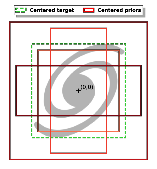
Figure 23: Illustration of a zero-centered comparison between a target in dashed green and different theoretical detection units in shades of red. This represents the classical YOLO association process in a grid cell.

To detect multiple small objects in a single grid cell, we need to have multiple detection units with comparable size priors. For this, we base our association function on the current position and size of the predicted box instead of their size priors. In such a case, the best theoretical associate would be counter-productive and force the network to make irrelevant associations. To illustrate this effect, we present in Fig. 24 a case with three target boxes and four predictions from independent detection units, all in the same grid cell, and the resulting association based on both the theoretical-prior association and the best current prediction association. We observe that the first one considers that no prediction is properly placed but that their size is relatively good, while the second one considers that the network is already relatively good at detecting the objects and that it is mostly the predicted size that needs to be adjusted.

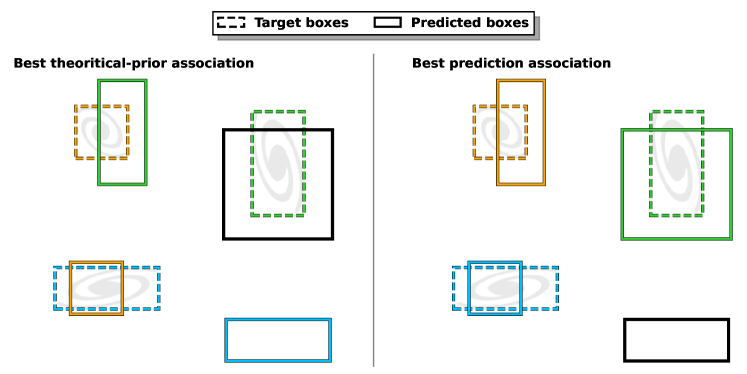
Figure 24: Comparison of the target-prediction association in a grid cell using two different association functions. The color indicates which prediction was associated with each target. The association results are illustrated for the default YOLO association function that is based on the best theoretical priors (left) and for an association function that uses the best current network prediction (right).

A.4 Box matching metric

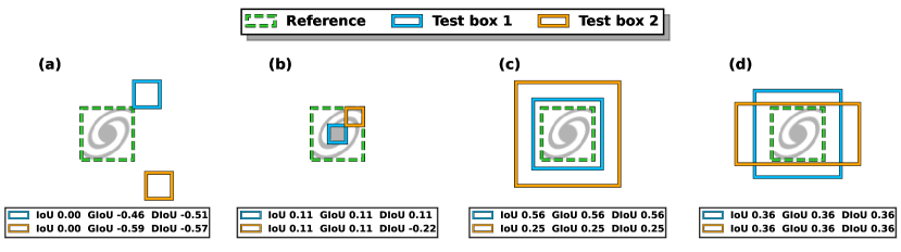
Figure 25: Comparison of three IoU-based metrics in different contexts. For all cases, the reference box is the dashed green box, and two test boxes in blue and orange are compared. The IoU-based metrics are always obtained by computing between a given case and the reference.

A prediction-aware association function has to be capable of selecting which prediction is the best current representation of the target. It means that we need a box-matching metric that is capable of discriminating between all the possible predictions in our specific context. The classical IoU matching criteria defined in Sect. 2.1 with Eq. 9 present strong limitations. To illustrate them, we compare IoU computations between a reference box and two possible test boxes in different contexts in Fig. 25. The main problem is that the IoU is equal to zero for all couple of boxes that have no intersection regardless of their distance (Fig. 25, frame A). For our specific astronomical applications where objects can be much smaller than the input size mapped by a grid cell, we need to be capable of attributing a different match score to non-intersecting boxes based on their distance to the reference. For this, we can use the Generalized IoU (GIoU, Rezatofighi et al. 2019) that makes use of the smallest box C that encloses the two boxes A and B to be compared by refining the default IoU following

$${\rm GIoU}={\rm IoU}-\frac{C-(A\cup B)}{C}.$$ (28)

The GIoU can take values from -1 to 1 while still being equal to the IoU in cases where C is equal to one of the two boxes. While leveraging the first limitation, the GIoU remains insufficient to distinguish between test boxes fully contained inside the reference box. In such a context, we would like to attribute a different match score based on the distance between the box centers (Fig. 25, frame B). For this, we can use the Distance IoU (DIoU, Zheng et al. 2019). This matching metric combines the classical IoU with the ratio between the distance of the box centers $A_{c}$ and $B_{c}$ and the smallest enclosing box diagonal-length $d$ in the form

$${\rm DIoU}={\rm IoU}-\frac{\rho^{2}(A_{c},B_{c})}{d^{2}},$$ (29)

where $\rho$ represents the Euclidean distance between the two center coordinates. The DIoU can take values from -1 to 1 while being equal to the IoU and GIoU in cases where the two boxes have the same center, corresponding to $\rho^{2}(A_{c},B_{c})=0$ (Fig. 25, frame C and D). This last metric is well suited for astronomical applications, but it remains limited in cases where the aspect ratio of the boxes matters. For example, all the metrics we described would give the same results for two test boxes with the same center and identical surface but different aspect ratios (Fig. 25, frame D). This could be included in a more refined matching metric like the Complete IoU (CIoU, Zheng et al. 2019).

We stress that all these IoU variants are only used as match criteria. The bounding-box-related loss remains a simple sum-of-square error on the box position and size following what was presented in Sect. 2.1 and Eqs. 6 and 7. This contrasts with what is described in the papers describing these metrics, where they are presented as alternative loss functions for object detection methods. In practice, all these matching metrics are implemented within YOLO-CIANNA and can be selected regarding the application. The predicted objectness uses the corresponding metric (re-scaled between 0 and 1 if necessary) to follow Eqs. 10 and 11, so the predicted score reflects all the related subtleties.

A.5 Association ordering effect

With multiple target objects and multiple predictions in the same grid cell, the association ordering starts to matter. In the original YOLO, it is done by looping over the target list for each grid cell. Having multiple targets on the same grid element would mean that they are very different in size, so they are considered unlikely to require the same detection unit. With an association process based on the current network prediction, any detection unit can be the best representation for any target regardless of its size prior. We defined our YOLO-CIANNA association function to be a search for the highest value in a matching score matrix that contains the ${\rm fIoU}$ for all the target-prediction pairs as described in Sect. 2.6. We illustrate the effect of such an association function compared to a loop over the targets and a loop over the predictions in Fig. 26. With our approach, if there are not enough detection units to accommodate all the targets, the well-detected objects will get associated first, which is not the case with the two approaches based on loops.

Interestingly, in the YOLO-V1 formalism, the output can be seen as a single grid cell of the size of the input image. This is due to the dense output layer and to the encoding of the predicted box center coordinates in a way that allows them to be positioned anywhere in the image regardless of the grid cell that predicts them. Therefore, all the association problems we identified when handling multiple objects per grid cell were also present in this V1 implementation but at the scale of the full image. We observe that several tricks similar to ours were used to mitigate the identified association issues. In particular, the association process at that time was based on the current predictions of the network instead of the best theoretical association. In a way, adopting a positioning system that forces each box to belong to a small grid element can be seen as a structural solution to the association issues, allowing the classical YOLO to switch to a non-prediction-aware association. Still, this solution alone is not viable for very small objects, as discussed in Sect. A.2.

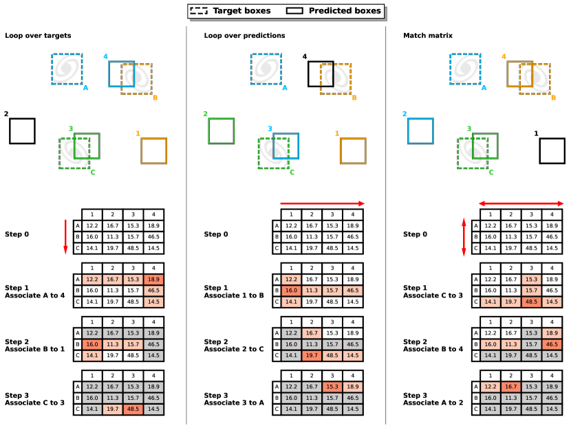
Figure 26: Comparison of the target-prediction association in a grid cell regarding the search order. The color indicates which prediction was associated with each target. All predictions and targets have the same size and shape, respectively. The prediction-target pairs are compared using a scaled $({\rm DIoU}+1){\times}0.5{\times}100$ and the results for all pairs are displayed in a matching matrix. For each step of the association process, the rows and columns corresponding to the targets and predictions are highlighted in light red, with the intersection being the match score for this pair. For all subsequent steps, the now unavailable elements in the matrix are shown in gray. The three frames compare different association results, along with the corresponding association steps highlighted in the match score matrix, when looping over the targets (left), looping over the predictions (middle), or searching for the maximum value in the score matrix (right).

A.6 Association refinements

Using a prediction-aware association implies that the network is free to try to distribute the diversity of objects over the detection units independently of their size prior. This added degree of freedom increases the training difficulty. Therefore, completely removing the theoretical box-prior association process is usually inefficient. This section describes several refinements we added to our default prediction-aware association process described in Sect. 2.6 to constrain the accessible solutions and guide the training process. Regarding our complete loss function (Eq. 14), these refinements will only affect the content of the $\mathds{1}^{match}$ and $\mathds{1}^{noobj}$ masks. Most of them occur after a target-prediction couple has been selected in the association search and are applied sequentially in a mutually exclusive way, following the blue B.2 frame in Fig. 4. Consequently, the association ordering matters, and a detection unit associated with a given target is not eligible as a possible solution for all the following targets, even during the refinement conditions. It also means that the current target-prediction pair found by the default association search is preserved if no box-prior that respects the different refinement conditions is available.

We emphasize that we describe all the available refinements in our method, whether or not they have been employed in the present study. Since most of them have a regularization effect, they can be useful to stabilize the training process while lowering the best achievable score. However, listing all the accessible refinement in the same place will allow future reference, and it should also allow other research teams to explore alternative efficient configurations that we might have missed.

A.6.1 Strict detection unit association

The first and most obvious refinement is to prevent some detection units from being associated with targets that are too different from their size prior. We do this by defining a ”strict association range” $S_{ar}$ that represents the number of detection units that are available to a target object of a given size. For example, with $S_{ar}=3$, each target can only be associated with the three detection units with the closest theoretical size priors. In practice, we do this by masking elements in the matching score matrix before starting the association process (A.3 frame in Fig. 4). The association is still based on the best current prediction but only using a subset of detection units. Interestingly, we can see the classical YOLO-V2 association process as a special case where $S_{ar}=1$.

For this selection to work, we must define which detection units best suit a given target. For this reason, we implemented three different theoretical proximity measurements. The first one is identical to YOLO-V2 and uses a zero-centered IoU comparison. The second one uses the Euclidean distance between the target and the prior of each detection unit in the 2D box-size space. The third one searches for the minimum absolute value for the target size by comparing what would be $\hat{o}_{w}$ and $\hat{o}_{h}$ for each detection, which is equivalent to measuring a distance in the exponentiated and prior-scaled size space. Our preference goes to the last definition as it is more directly related to the loss expression (Eq. 7). The classical zero-centered IoU was mainly kept so our method can emulate a classical YOLO association.

In the specific context of multiple small objects in the same grid cell, we might need to define multiple detection units with an identical size prior, as we did in Sect. 3.7.2. If that is the case, we consider that all detection units with identical priors are made available together and only count for a single $S_{ar}$ increment. For example, with a list of size-priors $p_{w}=p_{h}=\left[6,6,6,6,12,24\right]$ and $S_{ar}=2$, a square target of size $\hat{w}=\hat{h}=7$ could be associated to all the detection units except the one with the largest size prior. All the detection units with $p_{w}=p_{h}=6$ are considered to represent the same scale and account for the first $S_{ar}$ increment, and the second one is the single detection unit with $p_{w}=p_{h}=12$. With this definition, we can discriminate regarding size scales, with some of them being represented by more possible detection units than others. Ultimately, we expect detection units with identically sized priors to specialize based on criteria other than size or shape. By construction, we define that a value of $S_{ar}=0$ implies that this refinement is turned off and that all detection units are available.

A.6.2 Startup and forced random association

At the beginning of the training, when all the weights are still close to their initialization values, the network can be very sensitive to gradient explosion. In addition, the network can be prone to solution collapse, with only a few detection units actively trying to represent all the targets. Due to our prediction-aware association, it is more difficult to reintegrate the unconstrained detection unit as they are less likely to represent a good match than the already constrained ones. One solution to mitigate this issue is to have a low starting learning rate that progressively increases (Sect. 3.8). However, it works best when combined with a second solution, which is to deactivate the prediction-aware association for a given number of iterations $N_{rand}$ and perform a random target-prediction matching instead (B.2.1 frame in Fig. 4). With this method, each detection unit sees a variety of examples representative of the full training dataset distribution, which constrains them to a range of plausible values while preserving enough diversity to prevent solution collapse. These solutions are already part of some versions of the classical YOLO implementation.

For both the default YOLO and our adapted method, having our detection units specialize in some categories of objects is an efficient way to distribute the network expressivity. However, having mostly independent detection units might result in discontinuities in the predicted values for some object properties. This effect can be striking for additional parameters predicted with the formalism presented in Sect. 2.4. For example, when predicting a source flux, there is an overall scaling with the source size. Consequently, if the detection units are mostly distributed over the object size, they can only learn the corresponding subset of the flux relation. Having access to only a sub-part of the parameter space to be predicted can lead to poor constrain of the underlying function, especially on the edges of the sub-part interval.

Our method can ensure some representation overlap between our detection unit directly from the permissive association process when $S_{ar}>1$. However, this approach only allows representation overlap and does not guarantee it. As for random startup, forcing random associations would allow each detection unit to access parts of the underlying function outside its usual specific parameter sub-space. From this, we added the possibility of a random association at a user-defined rate $\alpha_{rand}$ (also B.2.1 frame in Fig. 4), which ensures better continuity of predicted parameters across all detection units. A side effect of this random association is that it acts as an additional training regularization and helps prevent solution collapse. A very low value for $\alpha_{rand}$ around one or two percent is usually enough to obtain a strong regularization effect. While this solution mitigates the apparition of discontinuities, it can still be observed for some of the parameters represented in Fig. 19 from Sect. 4.4, especially on $Bmaj$ and $Bmin$.

A.6.3 Forced specific detection unit association

For the same reasons we added the strict detection unit association (Appendix A.6.1), there are specific cases where stronger constraints can be beneficial. The first forced association is for small objects that are difficult to identify or position because their features are often badly resolved. Also, for small objects, higher precision is required on the positioning to achieve a given prediction-target overlap, which also means that the chances of a random match are low. For these reasons, it is often useful to force the association of very small objects with the detection unit with the smallest size prior in contexts where $S_{ar}>1$. Interestingly, this idea is also present in the YOLO-V1 but was abandoned after switching to the fully convolutional formalism in YOLO-V2. In our method, this forced association is made by comparing the target surface to a limit value that is defined as $\alpha_{small}{\times}s_{w}{\times}s_{h}$, with $s_{w}$ and $s_{h}$ the width and height of the smallest size-prior, and $\alpha_{s}$ a user-defined scaling factor (B.2.2 frame in Fig. 4). If multiple detection units have an identical size-prior that is the smallest, they are all considered viable options. The new target-prediction pair is selected by searching for the best current prediction in this subset of detection units. This is equivalent to having a special value of $S_{ar}=1$ for very small targets, regardless of the global value of $S_{ar}$.

The second forced association searches for the best theoretical detection unit. In our default association process, ordering the association following the matching score matrix helps to associate predictions with the target object they are actively trying to represent. On the contrary, this process is not helpful when a target object is not currently represented by any of the remaining predictions placed randomly in the background. For illustration, in Fig. 26, target A does not have any good association, and the choice to associate it with prediction 2 rather than prediction 1 is solely based on distance. While it can be a good criterion to select the current best prediction when it is actually trying to represent the object, it becomes less informative with predictions that are so far away that they do not represent anything and are likely random. In such a case, it might be better to associate the target with the available detection unit that should theoretically be the best suited to represent it. In this regard, the classical YOLO association, which is based solely on this principle, can be considered a good ”default” association when no assumption can be made regarding each prediction’s relevance other than its prior size. In our method, this forced association with the best theoretical detection unit is adopted when ${\rm fIoU}\leq L^{{\rm fIoU}}_{low}$ with ${\rm fIoU}$ the score of the current target-prediction pair and $L^{{\rm fIoU}}_{low}$ a user-defined threshold. When this refinement is triggered, it will search for the best theoretical prior as described in Appendix A.6.1 accounting for multiple identical priors and excluding already locked boxes (B.2.3 frame in Fig. 4). In addition, this refinement can also serve as a regularization by defining a user-defined rate $\alpha_{best}$ at which this refinement is applied regardless of the ${\rm fIoU}$ value for the current target-prediction pair. This specifically helps prevent solution collapse in cases where $S_{ar}$ is large by forcing all detection units to be used at some point. We found that $\alpha_{best}=0.05$ works well as a regularization for datasets based on everyday life images.

This last refinement can also be used in another way. By setting it to a high value up to $\alpha_{best}=0.95$ in association with a large $S_{ar}$, we are emulating a case where $S_{ar}=1$ but allowing another detection unit that is currently better at detecting a given object to get the association at a low $1-\alpha_{best}$ rate. This type of setup is especially useful for contexts with a strongly imbalanced scale distribution in the training sample, and it is also better at improving the continuity of the predicted parameters across the available detection units. We stress that this approach is very different from a setup with $S_{ar}=1$ and a low $\alpha_{rand}$ rate for which the quality of the current prediction would never matter.

A.6.4 Difficult flagging and quality check

All target objects are not equally difficult to detect, be it due to specific class features, apparent size, strong context dependency, partial obscuring from another object, or proximity to the edges of an image. Moreover, the detection difficulty is not a discrete property. From this, deciding if an object should be included as a target in the training sample regarding a specific application and set of objectives is complex. However, there are cases where both removing or keeping the object can degrade the network performance. For an object only partially visible on the edge of an image, the network might not always be capable of detecting it depending on the apparent features and the current network state. As exposed in Sect. 3.4, if we choose to remove the object while the network is confident in predicting its presence, it will be tasked to lower the objectness score of all objects with similar detectable features. In the opposite case, keeping an object while the network cannot identify any relevant feature will add a lot of noise to the training. This scenario is actually common, especially when performing data augmentation. A classical systematic approach for handling objects close to an edge is to keep them as targets if at least 50% of their expected size is visible in the input data. With this approach, the capability of the network to detect the object can strongly depend on which half is visible. For a target labeled as a cat, having its face visible with the associated features would be more valuable than having just its backside, which could be confused with the likely many similar classes in the training sample.

Several reasons could make an object difficult but not impossible to detect. For all these strongly application-dependent cases, we designed a ”difficult flag” that can be attributed to any target object and for which we apply a ”positive reinforcement only” update. Any target with this flag activated is considered a match if the network is confident enough in its current prediction. This is controlled by two user-defined thresholds based on the predicted box quality ${\rm fIoU}\geq L^{{\rm fIoU}}_{diff}$ and current confidence $O\geq L^{Obj}_{diff}$ of the network (B.2.4 frame in Fig. 4). If one of these limits is not fulfilled, we consider there is no match, but the target still counts for defining the GBNB masks. It means that a good match with low confidence is not penalized, allowing its confidence to increase with further training from similar targets. These limits are tested after all the association refinements, so if the quality condition is not fulfilled, the associated detection unit is considered free for subsequent associations.

Difficult objects are obviously difficult to detect but can also be difficult to classify or characterize. For example, predicting the flux of an astronomical source cut on the edge of the image requires the network to learn symmetrical assumptions that are only required and constrained for this specific context. It is sometimes better to rely on a confident target to properly define the interesting features and to only try to detect or characterize difficult objects based on resemblance. To encapsulate these subtleties, our difficult flag can take different values controlling which parameters get updated when the object passes the quality check: ”0” when the object is not difficult; ”1” when all the parameters should be updated; ”2” when the box geometry, objectness, and probability should be updated, but not the class nor the extra parameters; and ”3” when only the objectness and probability should be updated. All these flagging only affect training and are not reflected in the prediction outside the general objectness score.

A.7 YOLO-CIANNA cascading loss

In sect. 2.7, we introduced the concept of cascading loss, which refers to the fact that the loss varies during training as a function of the current state of the network prediction. This is a direct consequence of having a prediction-aware association in addition to various quality checks on the loss sub-parts and multiple association refinements. In practice, at the beginning of the training, the loss should be dominated by position and size updates toward the most obvious target objects. As the network improves for these objects, their respective loss term will lower, making the contribution from less obvious objects more dominant. Simultaneously, the obvious objects will become sufficiently well detected for other aspects like the objectness, the class, or the additional parameters to be included. From the loss perspective, it results in a competition between better characterizing the obvious objects and starting to detect less obvious ones.

In summary, the better the network gets, the more complete and complex the loss becomes. The objective is to order the network expressivity toward the most important aspects at a given point in the training, not bothering to adjust currently irrelevant properties. Looking at the evolution of the validation loss during training, we usually observe that the loss for the parameters with a quality threshold starts low, then increases before lowering again and reaching a first plateau. This behavior tends to repeat several times during the training with a lower increase and subsequent plateau with a smaller value each time, hence the ”cascading” name. The same behavior can also appear on objectness and probability independently of the fitting limits due to possible regime change in the object distribution over the detection units or simply due to the ”difficult” flagged objects being progressively integrated into the loss.

However, it becomes difficult to identify overtraining with a loss that does not monotonously decrease. To counter this, our implementation contains a parameter to select if the monitored loss on the validation datasets should include all the refinements and limits (”complete” loss) or not (”natural” loss). In the second case, only the base association process is maintained, all difficult objects are ignored, and all the loss parameters are computed for every association regardless of their quality. This usually results in a more classical loss behavior suitable for monitoring overtraining while keeping the cascading loss for the training dataset only. In Fig. 13, we use the ”natural” loss, so the cascading effect is not visible in the monitored validation loss.

A.8 Classical detection dataset benchmark

This section presents a quick summary of the results we obtained on classical object detection datasets using our YOLO-CIANNA method. This aims to validate that our implementation is at least on par with the classical YOLO-V2 performances for everyday images and that our modifications and refinements in the context of astronomical images have not impaired the capabilities of our method for other applications. Since our objective is to evaluate the effect of our low-level modifications, we tried to reproduce the darknet-19 architecture from YOLO-V2 as closely as possible. The later darknet-53 from YOLO-V3 is currently out of reach with CIANNA. We then present classical benchmark results of our slightly modified architecture on the ImageNet, Pascal VOC, and COCO datasets. We only present the most critical aspects of these benchmarks because analyzing them is not the scope of this paper. Still, all the corresponding scripts with all the parameters are provided on the CIANNA git repository and archived with the V1.0 release.

A.8.1 YOLO-CIANNA structural limitations

Our CIANNA framework can already build and train various CNN architectures. However, we still miss some currently widespread structural elements and optimization techniques. Indeed, the overall complexity and diversity of methods in the global ML research field pushed us to implement functionalities and capabilities regarding their usefulness for our specific subset of astronomical applications. We describe here two features that are missing to reproduce the YOLO-V2 and V3 architectures exactly, namely the batch normalization and the skip connections.

While network expressivity, and therefore predictive performance, is supposed to increase with the number of layers, there is a point where it becomes counterproductive to add more layers due to vanishing gradient issues during the training process. This problem is long known (Bengio et al. 1994), and many proposed improvements of deep neural network structures over the last decades were directly aimed at mitigating this issue (e.g., the rectified linear unit activation, Xu et al. 2015). One of the widely adopted mitigation techniques is based on inter-layer normalization. The most common is the batch normalization (BN, Ioffe & Szegedy 2015) that renormalizes the activation map elements of a given filter over the full current batch to have a common mean and variance that is learned during training. It homogenizes the training between layers, strongly mitigating the vanishing gradient issue, and it also regularizes the network over the batch content during training. While the first effect would be beneficial in our case to allow for deeper architecture, the second one pushes the network to ignore the absolute value of the activation map content and rather works only on relative contrast. We expected this to be at least partly detrimental for astronomical images with a large dynamic or when trying to predict pixel-value-dependent parameters like the source flux.

For this reason, the implementation of BN was postponed, and we rater focused on implementing a known alternative technique called group-normalization (GN, Wu & He 2018). It works by normalizing over the activation map elements of a given group of filters but independently for each image in a batch. It preserves the vanishing gradient mitigation principle while removing the regularization aspect. It was demonstrated that replacing all BN operations with GN usually leads to similar performances on many computer vision tasks (Wu & He 2018). Contrary to BN, it comes with an independent hyper-parameter, the group size $g_{s}^{l}$, that defines the number of filters $s$ to be normalized together at a giver layer $l$. Interestingly, implementing GN provides access to two other classical layer normalization methods that are specific cases of GN, the layer normalization with $g_{s}^{l}=N_{f}$ (Lei Ba et al. 2016) and the instance normalization with $g_{s}^{l}=1$ (Ulyanov et al. 2017).

Another typical way to construct deeper networks is to build skip-connections or residual connections (He et al. 2015). These two approaches counter the vanishing gradient problem by adding shortcuts between the layers. In both cases, the shortcut usually spans over a few layers considered as a block, and very deep architectures can be built by stacking several blocks. The network will be first trained as a shallower network to propagate the error up to the higher layers and then progressively get more layers involved to refine its solution with a higher expressivity. Currently, this process is missing from CIANNA, which limits the network depth for some applications. Still, we have not yet encountered an astronomical application for which this is the clear main limiting factor. The absence of skip-connections explains why we cannot reproduce large architectures like darknet-53 from YOLO-V3. In this regard, our emulation of the darknet-19 from YOLO-V2 is also a simplification as we miss the one skip-connect near the end of the network, which can have a significant impact on performances for small objects (Appendix A.8.5).

A.8.2 Mean average precision metric

The classical metric used for object detection tasks is the mean average precision (mAP). While mAP can refer to slightly different quantities depending on the challenge, they all usually rely on the computation of the area under a recall-precision curve. The mAP is analog to the receiver operating characteristic curve (ROC) but for object detection tasks. In practice, mAP computation works as follows. All object detectors are expected to produce a score for their detection and sort them for the full dataset. Each prediction is then flagged as a true detection or a false positive using a match criterion that is usually based on a threshold limit using the classical IoU (Sect. 2.1 and Eq. 9). From this ordered list of true and false detections, it is possible to construct a running precision and recall quantity. The constructed raw recall-precision curve can present local drops due to some high-confidence objects sometimes being flagged as false detections. Therefore, the curve is modified to respect $p(r)=\max_{\tilde{r}>r}p(\tilde{r})$. The average precision (AP) is then obtained by computing the integral over this interpolated precision-recall curve.

Usually, the AP is computed for each class individually. All the AP values are then averaged to construct a more general mAP score. For some challenges, mAP is computed for a single IoU value and expressed as mAP@IoU. For others, multiple IoU thresholds can be used independently or together to construct an averaged mAP over a given IoU range. Overall, this metric has the advantage of considering the full sensitivity of a given detector, which better represents the full discrimination capability between the background and the objects to detect (Sect. 5.1).

A.8.3 Imagenet classification pre-training

Following the description in Redmon & Farhadi (2016), we build a network backbone as similar as possible to the darknet-19 architecture, which comprises 19 convolutional layers and a few pooling layers. The main structural difference is that we use GN instead of BN. We first train this backbone on the ImageNet-2012 dataset (ILSVRC-2012, Russakovsky et al. 2015) composed of roughly 1.2 million single-label images with 1000 possible classes. This dataset’s size and diversity make it useful to pre-train networks to identify generic low-level features that are likely relevant for various applications. Due to the missing BN regularization, we must compensate with a more diverse data augmentation, still following common augmentation recipes. We first trained our network at the typical $224{\times}224$ input resolution up to a loss plateau that achieved a Top-1 accuracy of 70.1% and a Top-5 accuracy of 89.4$ on the validation dataset. We then further train the network at a $448{\times}448$ input resolution, which is closer to the desired input resolution for our object detectors that will use this model as pretraining. With access to finer features, the network achieved a Top-1 accuracy of 73.9 and a Top-5 accuracy of 91.9. For comparison, the classical darknet-19 architecture reaches a top-1 accuracy of 76.5% and a top-5 accuracy of 93.3%. The remaining difference is likely due to the absence of BN in our architecture, which results in a lack of appropriate regularization. When diverging slightly more from the original darknet-19 to include more regularization in another form, we can close the accuracy gap, for example, by adding multiple dense layers with a high dropout rate between the global average pooling and the output layer. The corresponding scripts with all the hyper-parameters and the testing notebook are available in the CIANNA git repository, along with example applications to images from the test dataset.

A.8.4 PASCAL-VOC object detection

The PASCAL-VOC (PASCAL Visual Object Classes, Everingham et al. 2010) dataset was a yearly computer vision challenge that ran from 2005 to 2012 and that included an object detection task. This dataset is still commonly used as a benchmark to compare the performances of different object detectors. One classical approach with this dataset is to combine the training and validation dataset from the 2007 and 2012 editions onto a single training sample and to evaluate the performances on the 2007 public test dataset of 5000 images or the 2012 hidden test dataset using the submission server. With this construction, the training set comprises roughly 16500 images with target bounding boxes of 20 possible classes. Using our high-resolution pre-trained backbone on ImageNet, we can drop the last pooling and output layer and add three new convolutional layers with $3{\times}3$ filters plus GN. Finally, we add our detection layer. The input resolution is also changed for a $416{\times}416$ input, which results in a $13{\times}13$ output grid. We note that in the original YOLO-V2 architecture, there is an additional skip connection between the second last layer and the layer just before the last pooling so that the network can access higher-resolution features for its prediction. As stated in Appendix A.8.1, the absence of this skip-connect will likely affect detection performances. While we could completely emulate the default YOLO association process, we use some of our method refinements to overcome the few structural limits we face. For example, we use the ${\rm DIoU}$ as matching score, $S_{ar}=3$, $L^{{\rm fIoU}}_{low}=-0.1$, $L^{{\rm fIoU}}_{C_{g}ood}=-0.1$, $\alpha_{best}=0.05$, and difficult object flagging. With these adjustments and a more diverse data augmentation, we achieve an ${\rm mAP@0.5}$ of 75.29% on the PASCAL 2007 test dataset. At the same resolution, the original YOLO-V2 model achieves 76.8%. Considering the structural limitations of our network that prevent us from perfectly emulating the original YOLO-V2 architecture, this result is a strong demonstration of the efficiency of our YOLO-CIANNA method. The corresponding scripts with all the hyper-parameters and the testing notebook are available in the CIANNA git repository, along with example applications to images from the test dataset.

A.8.5 COCO object detection

Table 6: Results comparison for COCO using the dedicated challenge metrics on the test-dev 2017 dataset.

	${\rm AP_{0.5:0.95}}$	${\rm AP_{0.5}}$	${\rm AP_{0.75}}$	${\rm AP_{S}}$	${\rm AP_{M}}$	${\rm AP_{L}}$	${\rm AR_{1}}$	${\rm AR_{10}}$	${\rm AR_{100}}$	${\rm AR_{S}}$	${\rm AR_{M}}$	${\rm AR_{L}}$
YOLO-V2	21.6	44.0	19.2	5.0	22.4	35.5	20.7	31.6	33.3	9.8	36.5	54.4
YOLO-CIANNA	22.2	40.1	22.2	4.1	22.9	38.3	20.8	30.3	31.3	4.4	34.5	55.4

The COCO (Common Objects in Context, Lin et al. 2014) dataset was also a yearly computer vision challenge that ran from 2014 to 2017, and that included an object detection task. Like PASCAL, the COCO is still commonly used as a benchmark to compare the performances of different object detectors. In the 2017 version, the training set comprises roughly 118000 images, the validation set comprises 5000 images, and the hidden test set comprises roughly 40000 images (accessible through a test server). For the detection task, the objects are labeled with over 1000 classes. We use the same network backbone with pretraining on ImageNEt, with the same set of hyper-parameters we used for PASCAL and a $416{\times}416$ input resolution. Our result on the test dataset obtained using the submission server is presented in Table 6 using all the COCO metrics and is compared with the result of the classical YOLO-V2. We first observe that our method is competitive with the classical YOLO-V2 detector on this dataset despite our structural limitations. In addition, these metrics indicate that our method retrieves more large objects and better reconstructs the objects it manages to detect. However, the lower ${\rm mAP@0.5}$ score indicates that we recover fewer objects overall. This is likely due to a poorer detection of small objects, confirmed by the small ${\rm AR_{S}}$ corresponding to recall at small scales. This result was expected, considering that we lack the ending skip connection to allow our method to preserve more resolved features at the detection layer. The corresponding scripts with all the hyper-parameters and the testing notebook are available in the CIANNA git repository, along with example applications to images from the test dataset.

Regarding computing performances, we can achieve 690 images per second at this resolution using an RTX 4090 GPU with mixed precision enabled. On a much lighter A2000 mobile GPU, we still reach above 60 images per second, meaning that our implementation is perfectly suited for real-time detection on modern entry-level hardware. We note that this level of performance is similar to the one achieved by the original YOLO-V2 darknet implementation if we consider the raw TFlops scaling between our GPU and the one they used in the corresponding paper.

Finally, we highlight that our result is far from the current top scores on the COCO dataset that use much stronger architectures, but it is not our scope to compete with them. The presented benchmarks validate the method for a given relatively light architecture. Most of the time, the architectures that are truly useful for astronomical datasets are quite shallow due to much less feature diversity and complexity, the main challenges being placed in other aspects of the method design.

Appendix B Classical YOLO-V2 backbone for SDC1

When first exploring the suitability of a given machine learning method to a new problem, the classical approach is to look at how this method was applied to a similar problem. This is especially true regarding network architectures and hyperparameters since exploring these aspects from scratch without prior knowledge of what type of architecture might be efficient can be extremely costly in terms of time and computing resources. In addition, if the new application is sufficiently close to other well-known applications of the same method, you can use pre-trained models to save some training time or improve the performance of your application. The global idea is that time and computing resources have already been invested in searching for the optimum architecture and hyper-parameters. We note that it is the approach used in Sortino et al. (2023) when testing the capability of a YOLO architecture on a source detection problem and that they concluded on improved results when using a pre-trained model. In fact, achieving apparently good results with known architectures or with pre-trained models does not guarantee that it is suited for the new application. In worst cases, it can even lead to the false conclusion that a specific approach usually tied to a given architecture is inefficient or unsuited for a specific application. To participate in this global discussion, we explore in this section the results we obtained on the SDC1 dataset using the classical YOLO-V2 darknet-19 architecture in a naive way and compare it to our reference result with our custom architecture.

B.1 Selection of architectures and training setups

While the classical YOLO-V2 formalism could be emulated with our implementation, doing a thorough and documented comparison of the individual effects of all the modifications we made one by one would be too complicated. Here, we preserved all the data preparation, training setup, hyper-parameters selection, detection units setup, and prediction pipeline construction that we defined in Sect. 3 and only modified the network backbone and the starting weights. As a consequence, the setup of the last layer remains identical to our reference setup. To achieve the desired 16 reduction factor, we needed to cut a part of the darknet-19 architecture due to its reduction factor of 32. The classical way to do that is to preserve the first layers before the reduction factor reaches 32. Applying this approach to the architecture we used to emulate darknet-19 for the classical VOC datasets in the previous appendix section allows us to preserve the first 13 convolutional layers.

To provide interesting comparative results, we used two slightly different architectures. The first one is similar to using the pre-trained ImageNet network and modifying it for object detection. It is done by adding three new sets of convolutional layers with 1024 filters of size $3{\times}3$ followed by a GN, starting after our cut in the darknet-19 architecture, and then adding our detection layer. The only differences are the location of the pre-train architecture cut and the fact that we use the COCO model as our pre-trained network, which was already a detection task. We refer to this first architecture as YOLO-V2-base. The second one uses the same pre-trained part but uses the head of our adapted architecture consisting of the last 4 layers in Fig. 11 instead of the typical YOLO head. This structure has a more progressive increase in size and includes dropout regularization. We refer to this second architecture as YOLO-V2-regul. It is important to note the YOLO-V2-regul architecture is composed of 14.4 million parameters, which is very similar to our custom architecture. In contrast, the YOLO-V2-base is almost twice the size with a total of 28.3 million parameters, which is explained by the differences in the last 4 layers. In terms of computing performances, the YOLO-V2-regul architecture has almost the same performances as our custom architecture, while the YOLO-V2-base is around 20% slower.

We performed two independent training for each architecture, the first using the pre-trained weights for the corresponding layers and the second from scratch with classical random weight initialization for all layers. It means that we have a total of four independent models to compare. We use the same prediction pipeline with the parameters described in Sect. 3.9 still with a $512{\times}512$ input resolution for the four of them.

B.2 Results and discussion

Table 7: . List of SDC1 scores and related properties for source catalogs from different architectures.

Method	$M_{s}$ (Score)	$N_{det}$	$N_{match}$	$N_{false}$	$N_{bad}\in N_{false}$	Purity	$\bar{s}$
YOLO-V2-regul-scratch	445093	688112	645626	42486	15070	93.83%	0.7552
YOLO-V2-base-pretrain	423077	665304	620685	44619	16003	93.29%	0.7535
YOLO-V2-regul-pretrain	411541	642153	600193	41960	13398	93.47%	0.7556
YOLO-V2-base-scratch	386395	644371	591039	53332	15020	91.72%	0.7440

The best score results for each of the four models are presented in Table 7. The best of these four models has a score $7\%$ lower than the best score achieved by our custom architecture, the latter reaching better scores after only 400 iterations (Fig. 13). We stress that the difference between these scores is always significantly larger than the score variability we observed over multiple training of the same setup with our reference architecture. This indicates that the observed ordering between these models is significant. We observe that for the YOLO-V2-base architecture, the pretraining improves the detection results, while it degrades it for the lighter YOLO-V2-regul architecture. The apparent flux distribution for these four models is very similar to our reference model. The main difference between these models is their completeness at a given purity, allowing some of them to detect more sources. We also note that these models can be ordered identically by their flux characterization score, which is coherent as the predicted flux accuracy is one of the match criteria.

Our interpretation of these results is that the truncated darknet-19 architecture is not adapted to our application and encapsulates too much expressivity to be properly constrained by our training data. It appears that the pretraining does not encapsulate relevant information but rather acts as a startup regularization by reducing the accessible parameter space, preventing the network from over-fitting. The training of the YOLO-V2-base-scratch model is very unstable as we observe variations of about 100000 points between successive control steps when continuing the training after the best score iteration, which is a striking demonstration of overfitting. This model exhibits the poor results of an unconstrained network, while the YOLO-V2-regul-scratch demonstrates that adding a small amount of structural regularisation solves this issue better than pretraining. In our opinion, the strongest demonstration of the irrelevance of the features learned on COCO for our problem is that the YOLO-V2-regul-scratch model significantly outperforms the YOLO-V2-regul-pretrain model. In addition, we tested a variety of alternative setups around our YOLO-V2-regul architecture by changing the number of layers that start from their pre-trained weights. From this, we observe that the best achievable score degrades as the number of pre-trained layers increases. In this regard, we consider the common empirical observation about obtaining better results using pre-trained models as incomplete and possibly misleading regarding the relevance of low-level features learned from everyday-life images for astronomical datasets (e.g., Sortino et al. 2023; Wu et al. 2019). In addition, pre-trained models do not necessarily train faster than the others on this specific application, which is another sign of the non-relevant features they are starting from.

Finally, achieving a better result with our custom backbone indicates that architectures that have been proved efficient on everyday-life images are not necessarily arranged in a way that is suited for extracting information in astronomical images. A striking difference between the two architectures is the absence of inter-layer normalization. We already identified in Sect. 3.6 that using GN between almost all layers in our custom architecture significantly reduces our best achievable score because it alters the absolute value of the input pixels, which contains information about the flux and the dynamic. Still, the presence of GN is not enough to explain the lower result of the YOLO-V2-regul-scratch model, highlighting that other architectural design choices matter.

Appendix C Alternative training area for the SDC1

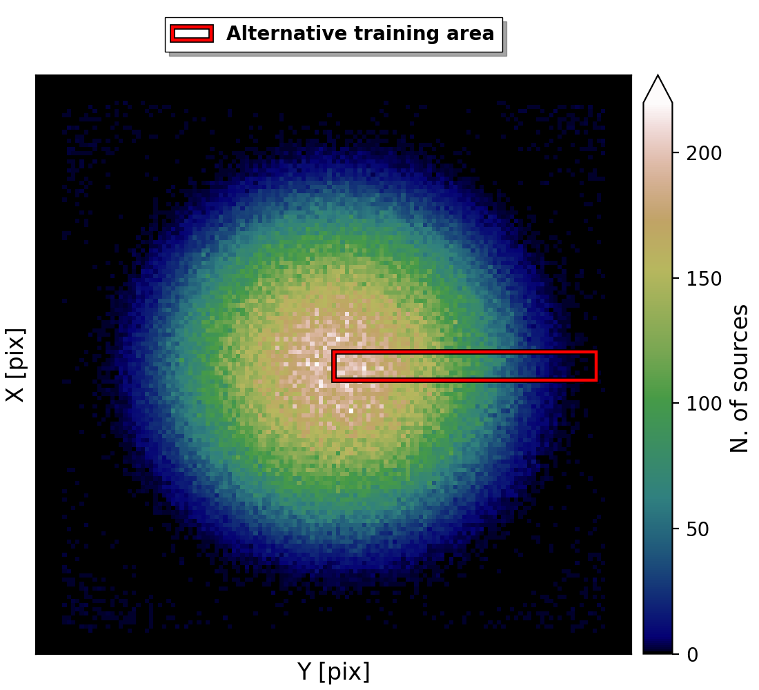
Figure 27: 2D histogram of the central coordinates of the sources from the full True catalog that passes our selection function. The red box indicates our modified SDC1 training area.

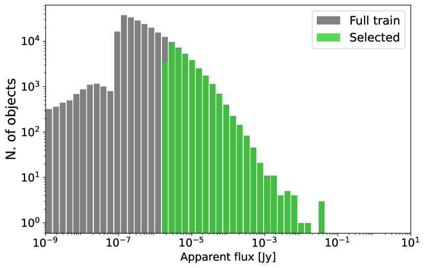
Figure 28: Source flux distribution histogram in log scale and using log-bins for the True catalog of the training region and the training catalog from our modified training area after the selection function.

Table 8: . List of scores and related properties based on the alternative training area for source catalogs from different architectures.

Method	$M_{s}$ (Score)	$N_{det}$	$N_{match}$	$N_{false}$	$N_{bad}\in N_{false}$	Purity	$\bar{s}$
YOLO-CIANNA-alt-train-large-bootstrap	502656	723655	690894	32761	12991	95.47%	0.7750
YOLO-CIANNA-alt-train-large	486053	709689	674404	35285	14380	95.02%	0.7730
YOLO-CIANNA-alt-train-ref	484145	708954	672906	36048	14988	94.91%	0.7731

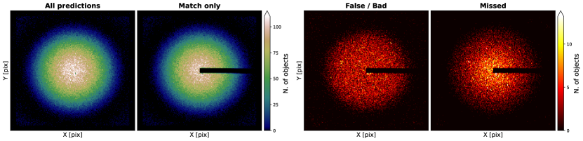
Figure 29: Distribution of various kinds of ”objects” over the full SDC1 field, minus our alternative training area when necessary, for the YOLO-CIANNA-alt-train-ref model. The match and false detections are based on the scorer, while the missed ones are based on our selection function. The central coordinates of the field are RA=0 deg, Dec=-30 deg.

We exposed in Sect. 3.5 the issues that arise from having access to only a small sub-part of the center of the full image to train our detector. Due to the convolution with the primary beam, the flux sensitivity varies in the image field, and this variation is impossible to represent with only the provided training region. We mitigated this issue by adding two regions of the image that we consider empty in our training sample to provide examples of noise-only fields. The results presented in Sect. 4 demonstrated that this approach allows the detector to perform relatively homogeneously on the whole image. This section explores how the result varies when using a training area more suited for supervised learning approaches regarding the image field variation.

C.1 Reference architecture

We use the post-challenge access to the full True catalog and define a new training area that spans from the center of the image up to the right edge, representing a radius of the primary beam. To evaluate only the effect of the training region, we need to preserve an identical number of examples. In practice, we adjust the thickness of the training radius to have a similar training sample size after selection than what we had in the default training area (Sect. 3.4). Our alternative training area is then a rectangular region with $-2.80\leq RA\leq 0.00$ degrees and $-30.12\leq Dec\leq-29.88$ degrees as illustrated in Fig. 27, and that contains 34913 selected sources that follow the flux distribution presented in Fig. 28. We observe that the amount of unselected sources at low apparent flux is much higher than for the reference catalog, which is simply an effect of having sources in all the primary beam sensitivity regimes from 1 to 0.

We train our network using the same configuration as our reference model and only change the training sample, which results in the YOLO-CIANNA-alt-train-ref model. The prediction is also made as before, but we had to alter the SDC1 scorer code to modify the training area definition. Using this modified code, we can obtain a score, presented in Table 8, and a list of matching sources to produce the same diagnostics as for our YOLO-CIANNA-ref catalog. While the scores cannot be directly compared due to the different testing areas, the number of detected sources is relatively similar to our YOLO-CIANNA-ref catalog. The purity is even slightly improved by 0.70%. The histogram of the apparent flux of the detected sources is presented in Fig. 31, exhibiting a similar distribution to our YOLO-CIANNA-ref result. The average source score is also slightly higher, resulting from a better source score that is likely the result of being provided with examples from all the primary beam regimes. Looking at individual fields produces results visually similar to our YOLO-CIANNA-ref model. However, looking at the distribution of false positive detections over the full image field from Fig. 29 demonstrates that our alternative training area results in a detector with more homogeneous detection performances. Overall, it demonstrates that this definition of training sample would have been a better representation of the image context by exhibiting better generalization results than our approach with the extra noise-only regions.

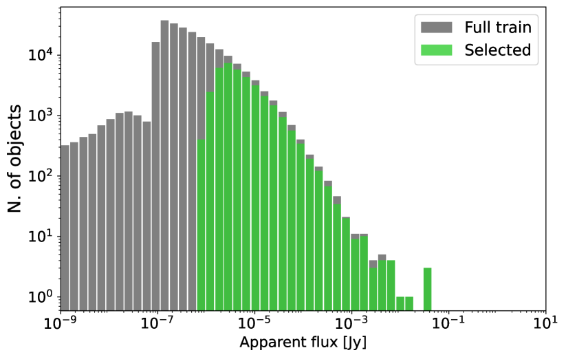
Figure 30: Source flux distribution histogram in log scale and using log-bins for the True catalog of the training region and the training catalog area after a single step of bootstrap refinement.

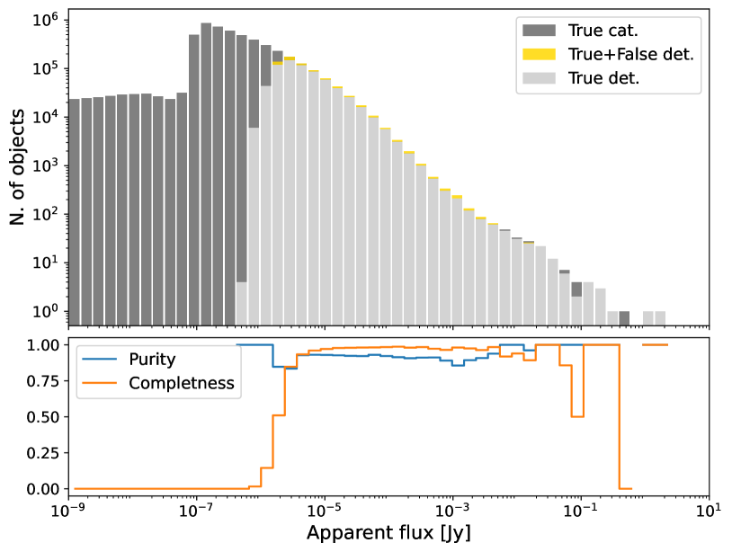
YOLO-CIANNA-alt-train-ref

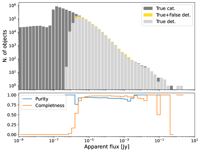
YOLO-CIANNA-alt-train-large-bootstrap

Figure 31: Histograms of the sources as a function of their apparent flux using logarithmic bins for the underlying True catalog and predicted sources in our modified testing area. The bottom part of each frame represents the purity and completeness of each bin of the histograms. The top frame is the results for the YOLO-CIANNA-alt-train-ref model, and the bottom frame is the YOLO-CIANNA-alt-train-large-bootstrap model.

C.2 Larger architecture and bootstrap training

An interesting side effect of this alternative training area is that the network training is slightly more stable. From this observation, we tried providing a bit of extra expressivity with less regularization by replacing the second last layer of our default architecture with two $1{\times}1$ convolutional layers, the first one with 3072 filters and a dropout of 30% and the second one with 2048 filters, constructing the YOLO-CIANNA-alt-train-large model. Training this new architecture with our alternative training area only modestly improves the score. This improvement can not be considered significant since it is of the same order as our typical multiple-training-identical-setup variability.

However, this network’s extra expressivity and stability make it suitable for testing the effect of a bootstrap approach for refining our selection function. In the following, we expose the main principle of this method, but it will be presented in more detail in the second paper of the series. The main idea is that instead of deciding which objects from the simulation should be considered detectable, we land this decision on the detector itself. This can be done by using a trained network on our hand-made selection function to make a prediction over the training region. The obtained detections can then be matched with the underlying list of real objects in the simulation to construct a new training sample. We stress that this process is never used to inject a network prediction as a new target directly. The properties from the True catalog sources that were successfully detected are used to define the new training sample. This approach requires stable training, as selecting a prediction before network convergence or when the network overtrains can harm the produced selection function. This approach can be repeated several times using the successively trained network detections to refine the selection function used for the next training.

We tested this approach on our reference model with the default SDC1 training area, but it did not improve the result significantly. With the default training area, any change in our hand-made selection function results in significant variations in the best achievable score. This variability comes mainly from the detections in the intermediate primary beam regime for which the network has to interpolate from the discontinuous training area. This effect is corrected with the alternative training sample, and the bootstrap training approach becomes useful. It is especially relevant in this context where the visibility of a source is strongly dependent on the beam regime, which was less the case when having access only to a central training area with less sensitivity variation. In such a context, having the network provide information on which sources can be considered visible is especially useful.

We apply this approach to our larger architecture and only do one bootstrap step. We present the resulting selection function in Fig. 30. Compared to our handmade custom function, it removes targets for almost all apparent flux values. The most plausible explanation is that it removes blended sources that are impossible to detect. Another effect is to smooth the low-cut flux in a larger flux interval. The score of the resulting model is indicated in Table 8, and the predicted sources flux distribution in Fig. 31. While all the diagnostics show results that are very similar to what we obtain with our reference architecture on our alternative training sample, we observe a significative score improvement of more than $3\%$, correlated with a better flux characterization score with $\bar{s}^{flux}=0.680$. More improvement would likely be achievable by searching the optimum architecture and hyper-parameters setup with this new training sample.

Overall, this approach removes the necessity for a well-defined selection function. This could be especially useful in a highly dimensional input space where defining a selection function by hand can be difficult. With this approach, the starting selection function could even be the catalog of a less performant detection method. Still, this approach requires access to all the possible targets regardless of their visibility, so only real detections are kept at each step. While a simulated dataset is the best-case scenario for this approach, it could still be employed on observed datasets by confirming the proposed detections with additional observations.