Mean field control of droplet dynamics with high order finite element computations

Abstract

Liquid droplet dynamics are widely used in biological and engineering applications, which contain complex interfacial instabilities and pattern formulation such as droplet merging, splitting, and transport. This paper studies a class of mean field control formulation towards these droplet dynamics. They are used to control and maintain the manipulation of droplets in applications. We first formulate the droplet dynamics as gradient flows of free energies in modified optimal transport metrics with nonlinear mobilities. We then design an optimal control problem for these gradient flows. We lastly apply the primal-dual hybrid gradient algorithm with high-order finite element methods to simulate the proposed mean field control problems. Numerical examples, including droplet formation, bead-up/spreading, transport, and merging/splitting on a two-dimensional spatial domain, demonstrate the effectiveness of the proposed mean field control mechanism.

1 Introduction

The dynamics of liquid droplets on solid substrates have been extensively investigated for the past two decades due to their significant connections to a wide range of biological and engineering applications, including heat and mass transfer (Ji & Witelski, 2018), vapor and particle capture (Sadeghpour et al., 2021, 2019), filtration and digital microfluidics (Kim, 2001). These droplet systems often exhibit complex pattern formation rendered by the interactions between the surface tension of the free interface and other physical effects. Fundamental droplet manipulation operations, such as droplet transport, merging, and splitting, have been explored experimentally through various mechanisms such as electrodewetting (Chu et al., 2023; Li et al., 2019), electrochemical oxidation (Khoshmanesh et al., 2017), and coalescence-induced propulsion (Jiang et al., 2022). Developing robust control mechanisms for droplet dynamics by varying external fields is essential to optimize the manipulation of droplets for practical applications. In this work, we will focus on mean field control of droplet dynamics in volatile thin liquid films.

Thin layers of viscous fluids spreading on solid substrates, often referred to as coating flows, have been studied in the context of tear films in human eyes and surface painting processes. When the solid substrate is hydrophobic or non-wetting, the fluid on the substrate spontaneously undergoes a sequence of instabilities and morphological changes, leading to the formation of dry spots and an array of interacting droplets. This fascinating dewetting phenomenon arises from the interplay of the intermolecular forces between the solid substrate and the fluid and the surface tension of the fluid.

In the limit of low Reynolds number, lubrication theory and thin-film models for free-surface flows have been widely used to model the droplet dynamics (Oron et al., 1997). Specifically, a classical long-wave thin-film equation can be cast into a gradient dynamics form (Thiele et al., 2016):

$$\frac{\partial h}{\partial t}=\nabla\cdot\left(V_{1}(h)\nabla\frac{\delta}{\delta h}\mathcal{E}(h)\right)-V_{2}(h)\frac{\delta}{\delta h}\mathcal{E}(h),\quad\text{ on }[0,T]\times\Omega,$$ (1.1)

where $h(t,x)$ represents the free surface height of the fluid film, $\mathcal{E}$ is an energy functional, and $V_{1}(h)\geq 0$ and $V_{2}(h)\geq 0$ are mobility functions associated with mass-conserving and non-mass-conserving contributions to the dynamics. We assume homogeneous Neumann boundary conditions $V_{1}(h)\nabla\frac{\delta}{\delta h}\mathcal{E}(h)\cdot\bm{\nu}=0$ on the domain boundary $\partial\Omega$, where $\bm{\nu}$ is the outward normal direction on $\partial\Omega$.

For a volatile thin-film on a hydrophobic substrate heated or cooled from below (Ji & Witelski, 2018; Ajaev & Homsy, 2001; Ajaev, 2005), vapor condensation or fluid evaporation occurs and leads to non-mass-conserving dynamics. In this case, typical mobility functions in (1.1) take the forms

$$V_{1}(h)=h^{3},\quad V_{2}(h)=\displaystyle\frac{\gamma}{h+K},$$ (1.2)

where $V_{1}(h)$ originates from the no-slip boundary condition at the liquid-solid interface, $V_{2}(h)$ term characterizes the non-mass-conserving liquid evaporation or condensation, $\gamma\geq 0$ is a phase change rate, $K>0$ is a kinetic parameter. The energy $\mathcal{E}(h)$ is given by

$$\mathcal{E}(h)=\int_{\Omega}\frac{\alpha^{2}}{2}|{\nabla{h}}|^{2}+U(h)\,dx\,,$$ (1.3)

where $\alpha>0$, and $U(h)$ is a local free energy relating to the wettability property of the substrate (Glasner & Witelski, 2003). When the substrate is dewetting or hydrophobic, the simplest forms of $U(h)$ and the corresponding disjoining pressure $\Pi(h)$ are given by

$$U^{\prime}(h)=\Pi(h)-\mathcal{P}_{*},\qquad\Pi(h)=\frac{\epsilon^{2}}{h^{3}}\left(1-\frac{\epsilon}{h}\right),$$ (1.4)

where $\mathcal{P}_{*}$ gives the influence of the temperature difference between the liquid film and the surrounding vapor phase. The parameter $\epsilon$ in $\Pi(h)$ sets a positive lower bound for the liquid height at which the attractive van der Waals forces balance with the short-range Born repulsion (Oron & Bankoff, 2001; Bertozzi et al., 2001; Ji & Witelski, 2018). The dynamic pressure $P$ of the free surface is given by

$$P(h)=\frac{\delta\mathcal{E}}{\delta h}=\Pi(h)-\mathcal{P}_{*}-\alpha^{2}{\nabla^{2}h},$$ (1.5)

where $\nabla^{2}h$ gives the linearized curvature of the free surface. We also have the following energy dissipation property:

$$\frac{d\mathcal{E}}{dt}=-\mathcal{I}(h)\leq 0,$$ (1.6)

where the dissipation rate

$$\mathcal{I}(h):=\int_{\Omega}\left(V_{1}(h)|\nabla P(h)|^{2}+V_{2}(h)|P(h)|^{2}\right)dx$$ (1.7)

is called the generalized Fisher information functional.

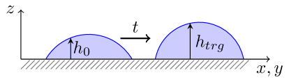
Figure 1: Schematic figure for the mean field control from the initial droplet profile $h_{0}(x,y)$ to the target droplet profile $h_{trg}(x,y)$.

Despite the wealth of modeling and analytical results on droplet dynamics, the field of controlling these free surface flows is still in its early stages of development. For instance, researchers have explored reduced-order-model-based control of liquid films governed by the classical Kuramoto-Sivashinsky (KS) equation, employing distributed control across the whole domain (Armaou & Christofides, 2000; Christofides & Armaou, 2000; Lee & Tran, 2005). Boundary control and optimal control of the KS equation have also been studied in the works of Katz & Fridman (2020); Al Jamal & Morris (2018); Coron & Lü (2015); Maghenem et al. (2022); Liu & Krstić (2001); Tomlin et al. (2019). However, the literature on controlling thin-film equations is relatively limited. For example, Klein & Prohl (2016) investigated optimal control of a simplified thin-film equation with only the fourth-order term. In the work of Samoilova & Nepomnyashchy (2019), the authors considered a linear proportional control for suppressing the Marangoni instability in a thin liquid film evolving on a plane. Cimpeanu et al. (2021) proposed an active control strategy of liquid film flows by incorporating information from reduced-order models. The work of Wray et al. (2022) focused on the electrostatic control for thin films underneath an inclined surface. Shankar et al. (2022) studied optimal transport and control of droplets of an active fluid. More recently, Biswal et al. (2024) studied the optimal boundary control of a thin-film equation describing thin liquid films flowing down a vertical cylinder. The mean field control of reaction-diffusion equations Mielke (2011); Fu et al. (2023a); Li et al. (2022a) and regularized conservation laws Li et al. (2023, 2022b) have been studied. In this direction, a recent work of Gao & Qi (2024) also discussed the control of coherent structures in turbulent flows using mean field games.

In this study, we demonstrate the application of mean field control (MFC) techniques for manipulating droplet dynamics within the framework of thin-film equations. The objective of MFC is to design and transport the droplets governed by the classical lubrication theory. See Figure 1 for an example of the transport and deformation of a droplet on a two-dimensional spatial domain from the initial surface height profile $h_{0}(x,y)$ to the target height profile $h_{trg}(x,y)$. We first illustrate the formulation of optimal control of thin-film equations as below. The constraint is given with the background of original physical dynamics, where the control variables contain both vector field and source terms with the above-mentioned nonlinear mobility functions $V_{1}(h)$ and $V_{2}(h)$. The minimization is then taken under the kinetic energy originating from the generalized Fisher information functional, adding suitable potential energy and terminal functionals. We then derive two equivalent formulations, for the latter one we develop the minimization systems of the proposed MFC problems in Proposition 2.1. They can be viewed as the forward-backward controlled systems of thin film dynamics.

We remark that the proposed MFC problem is motivated by the optimal transport theory (Villani, 2008). We study the optimal control problem associated with the gradient flow formulation from the thin-film equation in a generalized Wasserstein space. In particular, the control formulation itself is a generalization of the Benamou-Brenier formula (Benamou & Brenier, 2000), where we further consider the evolution of fluid dynamics under the thin-film equation as background. The proposed minimization system is the generalization of Wasserstein-2 type geodesics.

In simulations, our approach also utilizes high-order finite element computations to achieve this objective. Compared to previous work in Fu et al. (2023a), we remark that the second-order Laplacian term in the dynamic pressure $P$ in (1.5) brings additional difficulties in the simulation of proposed MFC problems. We construct several new constraints and Lagrange multipliers associated with primal-dual hybrid gradient methods Chambolle & Pock (2011); Carrillo et al. (2023) to handle the constraints associated with the dynamic pressure $P$.

The structure of the paper is as follows. In Section 2, we discuss the mean field control of droplet dynamics in thin-film equations. In Section 3, the high-order space-time finite element discretization and its associated primal-dual hybrid gradient optimization solver for the proposed mean field control problem is presented. Numerical results for the mean field control of droplet dynamics using the developed high-order finite element computations are presented in Section 4, followed by concluding remarks and discussions in Section 5.

2 Mean field control of droplet dynamics

This section presents the main formulation of mean field control (MFC) problems for the thin-film equation (1.1). We follow our previous work on MFC for (second-order) reaction-diffusion systems (Fu et al., 2023b). A byproduct of our MFC formulation is a new Jordan–Kinderlehrer–Otto (JKO) scheme for the PDE (1.1), which is similar to the variational time implicit scheme discussed in Fu et al. (2023a); see Remark 3 below.

Two new challenges emerge for MFC of (1.1). First, the energy functional (1.3) contains the gradient of the surface height, $\nabla h$, hence (1.1) is therefore a fourth-order PDE. Second, both mobility functions $V_{1}(h)$ and $V_{2}(h)$ are convex functions of $h$ (see (1.2)), which make the MFC problem a nonconvex optimization problem. The current work mainly focuses on the MFC formulation of droplet dynamics and its associated high-order finite element discretization. We will address the first challenge and show how the MFC framework for reaction-diffusion systems developed in Fu et al. (2023b) can be naturally adopted here using additional auxiliary variables. A corresponding high-order space-time finite element discretization and its solution procedure using the primal-dual hybrid gradient (PDHG) method will be presented in Section 3. We leave theoretical investigations on the (non)convexity issue of the proposed mean-field control problem for future work.

2.1 Droplet dynamics induced distances and MFCs

The energy dissipation law (1.6) and its associated Fisher information functional (1.7) naturally induce a metric distance between two positive surface heights $h_{0}$ and $h_{1}$, as we define in the following.

Definition 1 (Distance functional)

Define a distance functional $\mathrm{Dist}_{V_{1},V_{2}}\colon\mathcal{M}\times\mathcal{M}\rightarrow\mathbb{R}_{+}$ as below, where the space $\mathcal{M}=\{h\in L^{1}(\Omega):h\geq 0\}$. Consider the following optimal control problem:

$$\mathrm{Dist}_{V_{1},V_{2}}(h_{0},h_{1})^{2}:=\inf_{h,\bm{v}_{1},v_{2}}\quad\int_{0}^{T}\int_{\Omega}\left(|\bm{v}_{1}|^{2}V_{1}(h)+|v_{2}|^{2}V_{2}(h)\right)dxdt,$$ (2.1a)

where the infimum is taken among $$h(t,x)\colon[0,1]\times\Omega\rightarrow\mathbb{R}_{+} \bm{v}_{1}(t,x)\colon[0,1]\times\Omega\rightarrow\mathbb{R}^{d} v_{2}(t,x)\colon[0,1]\times\Omega\rightarrow\mathbb{R} h \bm{v}_{1} V_{1} v_{2} V_{2} h_{0} h_{1}\in\mathcal{M}$$, , , such that satisfies a reaction-diffusion type equation with drift vector field , drift mobility , reaction rate , reaction mobility , connecting initial and terminal surface heights , :

$$\left\{\begin{aligned} &\partial_{t}h+\nabla\cdot(V_{1}(h)\bm{v}_{1})=V_{2}(h)v_{2},\quad(t,x)\in[0,1]\times\Omega,\\ &h(0,x)=h_{0}(x),\quad h(1,x)=h_{1}(x),\end{aligned}\right.$$ (2.1b)

with no-flux boundary condition $$V_{1}(h)\bm{v}_{1}\cdot\bm{\nu}|_{\partial\Omega}=0$$.

Using the above-defined distance functional, together with the thin-film equation (1.1), we define the following mean field control (MFC) problem for droplet dynamics.

Definition 2 (MFC for droplet dynamics)

Give a time domain $[0,T]$, $T>0$, a potential functional $\mathcal{F}\colon\mathcal{M}\rightarrow\mathbb{R}$, and a terminal functional $\mathcal{G}\colon\mathcal{M}\rightarrow\mathbb{R}$,

consider

$$\begin{split}&\inf_{h,\bm{v}_{1},v_{2}}\int_{0}^{T}\!\!\left[\int_{\Omega}\frac{1}{2}\left(|\bm{v}_{1}|^{2}V_{1}(h)+|v_{2}|^{2}V_{2}(h)\right)dx-\mathcal{F}(h)\right]\!dt+\mathcal{G}(h(T,\cdot)),\end{split}$$ (2.2a)

where the infimum is taken among $$h(t,x)\colon[0,T]\times\Omega\rightarrow\mathbb{R}_{+} \bm{v}_{1}(t,x)\colon[0,T]\times\Omega\rightarrow\mathbb{R}^{d} v_{2}(t,x)\colon[0,T]\times\Omega\rightarrow\mathbb{R}$$, , , such that

$$\partial_{t}h+\nabla\cdot(V_{1}(h)\bm{v}_{1})-V_{2}(h)v_{2}=\beta\left[\nabla\cdot(V_{1}(h)\nabla P(h))-V_{2}(h)P(h)\right],$$ (2.2b)

with boundary condition

$$\left.V_{1}(h)(\bm{v}_{1}-\beta\nabla P(h))\cdot\bm{\nu}\right|_{\partial\Omega}=0,$$ (2.2c)

and initial surface height $$h(0,\cdot)=h_{0} \Omega \beta\geq 0$$ in . Here is a non-negative number, which represents the strength of the droplet dynamics (1.1) in the constraint of mean field control problem (2.2).

Remark 3 (JKO temporal discretization to (1.1))

In the above definition, if we take $T=1$, $\mathcal{F}=0$ and $\mathcal{G}(h)=\Delta t\mathcal{E}(h)$ as in (1.3), and set parameter $\beta=0$, we obtain a dynamic formulation of the celebrated JKO temporal discretization scheme Jordan et al. (1998) for the gradient flow (1.1), which is a first-order variational time-implicit discretization with stepsize $\Delta t>0$. See Fu et al. (2023a); Carrillo et al. (2022); Li et al. (2020) for a related discussion on JKO-type discretizations for gradient flows in Wasserstein-type metric spaces.

We remark that most existing works on thin-film control focus on the mass-conserving case with $V_{2}\equiv 0$. Our framework can be applied to both mass-conserving and non-mass-conserving $V_{2}\neq 0$ scenarios. Here, we illustrate a few examples considered in the literature.

Example 4

The work of Klein & Prohl (2016) addresses the optimal control problem in divergence form,

$$\partial_{t}h=\partial_{x}(\lambda|h|^{a}\partial_{x}P)+\partial_{x}u,\quad P=-h_{xx},$$ (2.3)

where $u(t,x)$ is the external control, $a>1$, $\lambda>0$. This problem is related to the MFC problem (2.2b) with $V_{1}=\lambda|h|^{a}$, $V_{2}\equiv 0$, $\bm{v}_{1}=-u/V_{1}$, and $\beta=1$. Such problem can be applied to the control of thin film deposition on silicon wafers during electronic chip fabrication.

Example 5

The work of Samoilova & Nepomnyashchy (2019) aimed to suppress the Marangoni instability in a thin film heated from below using a lubrication equation

$$\partial_{t}h=\nabla\cdot\left[\tfrac{1}{3}h^{3}\nabla P+\tfrac{Ma}{2}h^{2}\nabla(\Theta-h)\right],$$ (2.4)

coupled with a heat transfer equation for the controlled temperature $\Theta$. One can rewrite (2.4) into the form of (2.2b) by setting $V_{1}=h^{3}/3$, $V_{2}\equiv 0$, $\bm{v}_{1}=\tfrac{3Ma}{2h}\nabla(h-\Theta)$, and $\beta=1$.

Example 6

In the recent work on optimal transport and control of active droplet by Shankar et al. (2022), the active droplet is modelled by

$$\partial_{t}h=\partial_{x}\left[\tfrac{1}{3\eta}h^{3}(\partial_{x}P-\zeta h)\right],\quad P=-\gamma h_{xx},$$ (2.5)

where $\zeta(t,x)$ represents the controllable activity of suspension in the droplet. Again, this problem corresponds to (2.2b) with $V_{1}=h^{3}/(3\eta)$, $V_{2}\equiv 0$, $\bm{v}_{1}=\zeta h$, and $\beta=1$.

2.2 MFC reformulations

In this subsection, we focus on reformulations of the MFC problem in Definition 2 which will be suitable for a finite element discretization.

The first reformulation converts the constraint PDE (2.2b) to a linear constraint by a change of variables. Specifically, introducing the flux function $\bm{m}(t,x)\colon[0,T]\times\Omega\rightarrow\mathbb{R}^{d}$ and source function $s(t,x)\colon[0,T]\times\Omega\rightarrow\mathbb{R}$, such that

$$\bm{m}=V_{1}(h)\Big{[}\bm{v}_{1}-\beta\nabla P(h)\Big{]},\quad s=V_{2}(h)\Big{[}v_{2}-\beta P(h)\Big{]},$$ (2.6)

then the MFC problem (2) is equivalent to the following linearly constrained optimization problem: Given a potential functional $\mathcal{F}\colon\mathcal{M}\rightarrow\mathbb{R}$, and a terminal functional $\mathcal{G}\colon\mathcal{M}\rightarrow\mathbb{R}$, consider

$$\begin{split}\inf_{h,\bm{m},s}&\int_{0}^{T}\!\int_{\Omega}\tfrac{1}{2}|\tfrac{\bm{m}}{V_{1}(h)}+\beta\nabla P(h)|^{2}V_{1}(h)dxdt\\ &\!\!\!\!\!\!+\int_{0}^{T}\!\int_{\Omega}\tfrac{1}{2}|\tfrac{s}{V_{2}(h)}+\beta P(h)|^{2}V_{2}(h)dxdt-\int_{0}^{T}\mathcal{F}(h)dt+\mathcal{G}(h(T,\cdot)),\end{split}$$ (2.7)

where the infimum is taken among functions $h,\bm{m},s$, such that

$$\partial_{t}h+\nabla\cdot\bm{m}-s=0\;\text{ on }[0,T]\times\Omega,\;\left.\bm{m}\cdot\bm{\nu}\right|_{[0,T]\times\partial\Omega}=0,\;h(0,x)=h_{0}(x).$$ (2.8)

Expanding the product terms in (2.7), we get

$$\begin{split}\inf_{h,\bm{m},s}&\int_{0}^{T}\!\int_{\Omega}\left(\frac{|\bm{m}|^{2}}{2V_{1}(h)}+\frac{|s|^{2}}{2V_{2}(h)}\right)+\beta\left(\bm{m}\cdot\nabla P(h)+s\cdot P(h)\right)dxdt\\ &+\int_{0}^{T}\!\int_{\Omega}\frac{\beta^{2}}{2}\left(|\nabla P(h)|^{2}V_{1}(h)+|P(h)|^{2}V_{2}(h)\right)dxdt\\ &-\int_{0}^{T}\mathcal{F}(h)dt+\mathcal{G}(h(T,\cdot)).\end{split}$$

Using integration by parts and the constraint (2.8), we have

$$\int_{0}^{T}\!\int_{\Omega}\left(\bm{m}\cdot\nabla P(h)+s\cdot P(h)\right)dxdt$$

$$= \;\int_{0}^{T}\!\int_{\Omega}P(h)\left(-\nabla\cdot\bm{m}+s\right)dxdt$$

$$= \;\int_{0}^{T}\!\int_{\Omega}P(h)\partial_{t}h\;dxdt=\mathcal{E}(h(T,\cdot))-\mathcal{E}(h_{0}),$$

where we used the definition of dynamic pressure $P(h)=\tfrac{\delta\mathcal{E}(h)}{\delta h}$ in the last step. Combining these derivations and noticing that $h_{0}$ is given, we arrive at the following equivalent formulation of the MFC problem (2).

Definition 7 (MFC reformation I)

Consider

$$\begin{split}\inf_{h,\bm{m},s}&\quad\int_{0}^{T}\int_{\Omega}\left(\frac{|\bm{m}|^{2}}{2V_{1}(h)}+\frac{|s|^{2}}{2V_{2}(h)}\right)dxdt\\ &+\int_{0}^{T}\!\int_{\Omega}\frac{\beta^{2}}{2}\left(|\nabla P(h)|^{2}V_{1}(h)+|P(h)|^{2}V_{2}(h)\right)dxdt\\ &-\int_{0}^{T}\mathcal{F}(h)dt+\mathcal{G}(h(T,\cdot))+\beta\mathcal{E}(h(T,\cdot)),\end{split}$$ (2.9)

where the infimum is taken among $h,\bm{m},s$ satisfying (2.8).

Proposition 2.1 (MFC systems of droplet dynamics)

Let $(h,\bm{m},s)$ be the critical point system of the MFC problem (2.9). Then there exists a function $\phi\colon[0,T]\times\Omega\rightarrow\mathbb{R}$, such that

$$\frac{\bm{m}(t,x)}{V_{1}(h(t,x))}=\nabla\phi(t,x),\quad\frac{s(t,x)}{V_{2}(h(t,x))}=\phi(t,x),$$

and

$$\left\{\begin{aligned} &\partial_{t}h(t,x)+\nabla\cdot(V_{1}(h(t,x))\nabla\phi(t,x))-V_{2}(h(t,x))\phi(t,x)=0,\\ &\partial_{t}\phi(t,x)+\frac{1}{2}\|\nabla\phi(t,x)\|^{2}V_{1}^{\prime}(h(t,x))+\frac{1}{2}|\phi(t,x)|^{2}V^{\prime}_{2}(h(t,x))\\ &\hskip 165.02606pt+\frac{\delta}{\delta h}\Big{[}\mathcal{F}(h)-\frac{\beta^{2}}{2}\mathcal{I}(h)\Big{]}(t,x)=0,\end{aligned}\right.$$ (2.10)

where $\mathcal{I}(h)$ is the generalized Fisher information functional given in (1.7), such that

$$\begin{split}\frac{\delta}{\delta h}\mathcal{I}(h)=&\quad\frac{1}{2}(V_{1}^{\prime}(h)|\nabla P(h)|^{2}+V_{2}^{\prime}(h)|P(h)|^{2})-\nabla\cdot(V_{1}(h)\nabla P(h))\Pi^{\prime}(h)\\ &+\alpha^{2}\Delta\nabla\cdot(V_{1}(h)\nabla P(h))+\Pi^{\prime}(h)V_{2}(h)P(h)-\alpha^{2}\Delta(P(h)V_{2}(h)),\end{split}$$

with initial and terminal time conditions

$$h(0,x)=h_{0}(x),\quad\phi(T,x)=-\frac{\delta}{\delta h}\Big{(}\mathcal{G}(h(T,\cdot))+\beta\mathcal{E}(h(T,\cdot))\Big{)}.$$ (2.11)

We remark that a similar MFC formulation and system for reaction-diffusion equation was considered in our earlier work (Fu et al., 2023a). We present the derivation of the MFC system (2.10) in the Appendix A.

MFC problems and systems are generalizations of Benamou-Brenier formulas in optimal transport (Villani, 2008). This refers to setting $\beta=0$, $V_{1}(h)=h$, and $V_{2}(h)=0$. In the context of mean field control of droplet dynamics, we need to address additional challenges, in which the dynamic pressure $P(h)$ given in (1.5) involves a second-order Laplacian term. This Laplacian term brings additional difficulties in using the finite element method to compute the proposed MFC problem. We also comment that the dynamic pressure $P(h)$ is essential in modeling the disjoining pressure and surface tension that governs the droplet dynamics. In numerical experiments, we demonstrate that the MFC problem with this pressure term exhibits essential patterns of droplets, including droplet spreading, transport, merging, and splitting.

We introduce additional auxiliary variables to further reformulate the MFC problem (7). Let $\bm{n}(t,x):[0,T]\times\Omega\rightarrow\mathbb{R}^{d}$, $p(t,x):[0,T]\times\Omega\rightarrow\mathbb{R}$, and $\bm{q}(t,x):[0,T]\times\Omega\rightarrow\mathbb{R}^{d}$ be defined as follows:

$$\bm{n}=\alpha\nabla h,\;\;p=-\alpha\nabla\cdot\bm{n},\;\;\bm{q}=\alpha\nabla p.$$ (2.12)

This implies $p=-\alpha\nabla\cdot(\alpha\nabla h)=-\alpha^{2}\nabla^{2}h$. Hence, the dynamic pressure satisfies $P(h)=U^{\prime}(h)+p$, and its gradient follows

$$\nabla P(h)=U^{\prime\prime}(h)\nabla h+\nabla p=\frac{1}{\alpha}(U^{\prime\prime}(h)\bm{n}+\bm{q}).$$

Plugging these relations back to the MFC problem (2.9), we obtain the following equivalent reformulation.

Definition 8 (MFC reformation I​I)

Consider

$$\begin{split}\inf_{h,\bm{m},s,\bm{n},p,\bm{q}}&\int_{0}^{T}\!\int_{\Omega}\left(\frac{|\bm{m}|^{2}}{2V_{1}(h)}+\frac{|s|^{2}}{2V_{2}(h)}\right)dxdt\\ &\!\!\!\!\!\!\!\!\!\!\!\!\!\!\!\!+\int_{0}^{T}\!\int_{\Omega}\frac{\beta^{2}}{2}\left(\tfrac{|U^{\prime\prime}(h)\bm{n}+\bm{q}|^{2}}{\alpha^{2}}V_{1}(h)+|U^{\prime}(h)+p|^{2}V_{2}(h)\right)dxdt\\ &\!\!\!\!\!\!\!\!\!\!\!\!\!\!\!\!-\int_{0}^{T}\mathcal{F}(h)dt+\mathcal{G}(h(T,\cdot))+\beta\int_{\Omega}\left(U(h(T,x))+\frac{|\bm{n}(T,x)|^{2}}{2}\right)dx,\end{split}$$ (2.13)

where the infimum is taken among $h,\bm{m},s$ satisfying (2.8), and $\bm{n},p,\bm{q}$ satisfying (2.12).

To simplify the notation, we collect the variables into a big vector

$$\bm{u}:=(h,\bm{m},s,\bm{n},p,\bm{q}),$$ (2.14)

and introduce $\bm{u}_{T}:=(h_{T},\bm{n}_{T})$ where $h_{T}:\Omega\rightarrow\mathbb{R}_{+}$ is the terminal surface height, and $\bm{n}_{T}:\Omega\rightarrow\mathbb{R}^{d}$ the scaled surface height gradient at terminal time. Hence $\bm{u}(t,x):[0,T]\times\Omega\rightarrow\mathbb{R}^{3d+3}$ is a space-time function with $3d+3$ components, and $\bm{u}_{T}(x):\Omega\rightarrow\mathbb{R}^{d+1}$ is a spatial function with $d+1$ components. We further denote the functionals $H(\bm{u})$ and $H_{T}(\bm{u}_{T})$, such that

$$H(\bm{u}):= \;\frac{|\bm{m}|^{2}}{2V_{1}(h)}+\frac{|s|^{2}}{2V_{2}(h)}+\frac{\beta^{2}}{2\alpha^{2}}|U^{\prime\prime}(h)\bm{n}+\bm{q}|^{2}V_{1}(h)$$ (2.15a)

$$\;+\frac{\beta^{2}}{2}|U^{\prime}(h)+p|^{2}V_{2}(h)-F(h),$$ (2.15b)

$$H_{T}(\bm{u}_{T}):= \;\beta\left(U(h_{T})+\frac{|n_{T}|^{2}}{2}\right)+G(h_{T}),$$ (2.15c)

where $F(h)$ and $G(h)$ are density functions for functionals $\mathcal{F}$ and $\mathcal{G}$, i.e.,

$$\mathcal{F}(h)=\int_{\Omega}F(h)dx,\quad\mathcal{G}(h)=\int_{\Omega}G(h)dx.$$

Using these notations, the MFC problem 8 takes the following compact form:

Definition 9 (MFC problem: compact form)

Consider

$$\begin{split}\inf_{\bm{u},\bm{u}_{T}}&\int_{0}^{T}\!\int_{\Omega}H(\bm{u})dxdt+\int_{\Omega}H_{T}(\bm{u}_{T})dx,\end{split}$$ (2.16a)

subject to the constraints on the space-time domain

$$\begin{split}\partial_{t}h+\nabla\cdot\bm{m}-s=&\;0,\\ -\bm{n}+\alpha\nabla h=&\;0,\\ p+\alpha\nabla\cdot\bm{n}=&\;0,\\ \bm{q}-\alpha\nabla p=&\;0,\end{split}\quad\quad\quad\text{ on }[0,T]\times\Omega,$$ (2.16b)

and the constraints at terminal time

$$\begin{split}h(0,\cdot)=h_{0},\\ h(T,\cdot)=h_{T},\\ -\bm{n}_{T}+\alpha\nabla h_{T}=&\;0,\\ \end{split}\quad\quad\quad\text{ on }\Omega,$$ (2.16c)

with Neumann boundary condition

$$\bm{m}\cdot\bm{\nu}=0\quad\text{ on }[0,T]\times\partial\Omega.$$ (2.16d)

Remark 10

We note that all the MFC formulations above are mathematically equivalent. Our numerical discretization, however, will be constructed based on the last formulation in Definition 8 or Definition 9. It has a form that the constraints are linear PDEs, and the objective function does not involve spatial derivatives. These two properties are crucial for the efficient implementation of the finite element scheme that we will develop in Section 3.

2.3 Saddle-point problem

Finally, we reformulate the constrained optimization problem in Definition 9 into a saddle-point problem using Lagrange multipliers, for which a finite element discretization will be developed in Section 3. We introduce the following four Lagrange multipliers on the space-time domain $[0,T]\times\Omega$ for the four equations in (2.16b). They are scalar functions $\phi(t,x):[0,T]\times\Omega\rightarrow\mathbb{R}$, $\xi(t,x):[0,T]\times\Omega\rightarrow\mathbb{R}$, vectorial functions $\bm{\sigma}(t,x):[0,T]\times\Omega\rightarrow\mathbb{R}^{d}$, $\bm{\theta}(t,x):[0,T]\times\Omega\rightarrow\mathbb{R}^{d}$, and a Lagrange multiplier $\bm{\sigma}_{T}(x):\Omega\rightarrow\mathbb{R}^{d}$ on the spatial domain (at terminal time):

$$\partial_{t}h+\nabla\cdot\bm{m}-s= \;0 \;\;\longleftrightarrow\phi,$$

$$-\bm{n}+\alpha\nabla h= \;0 \;\;\longleftrightarrow\bm{\sigma},$$

$$p+\alpha\nabla\cdot\bm{n}= \;0 \;\;\longleftrightarrow\xi,$$

$$\bm{q}-\alpha\nabla p= \;0 \;\;\longleftrightarrow\bm{\theta},$$

$$-\bm{n}_{T}+\alpha\nabla h_{T}= \;0 \;\;\longleftrightarrow\bm{\sigma}_{T}.$$

Then the MFC problem 9 can be formulated as the following saddle-point problem:

$$\begin{split}\inf_{\bm{u},\bm{u}_{T}}\sup_{\bm{\Phi},\bm{\sigma}_{T}}&\quad\int_{0}^{T}\!\int_{\Omega}H(\bm{u})dxdt+\int_{\Omega}H_{T}(\bm{u}_{T})dx\\ &+\int_{0}^{T}\!\int_{\Omega}\Big{[}(\partial_{t}h+\nabla\cdot\bm{m}-s)\phi+(-\bm{n}+\alpha\nabla h)\cdot\bm{\sigma}\Big{]}dxdt\\ &+\int_{0}^{T}\!\int_{\Omega}\Big{[}(p+\alpha\nabla\cdot\bm{n})\xi+(\bm{q}-\alpha\nabla p)\cdot\bm{\theta}\Big{]}dxdt\\ &+\int_{\Omega}(-\bm{n}_{T}+\alpha\nabla h_{T})\cdot\bm{\sigma}_{T}dx,\end{split}$$

with the following boundary and initial/terminal conditions

$$h(0,\cdot)=h_{0},\;\;h(T,\cdot)=h_{T}\quad\text{ in }\Omega,\quad\text{ and }\bm{m}\cdot\bm{\nu}=0\text{ on }[0,T]\times\partial\Omega.$$

Here $\bm{\Phi}=(\phi,\xi,\bm{\sigma},\bm{\theta})$.

Next, applying integration by parts on the above saddle-point problem to move all derivatives of $\bm{u}$ to the dual variables $\bm{\Phi}$, and using the initial and boundary conditions, we obtain

$$\begin{split}\inf_{\bm{u},\bm{u}_{T}}\sup_{\bm{\Phi},\bm{\sigma}_{T}}&\int_{0}^{T}\!\int_{\Omega}H(\bm{u})dxdt+\int_{\Omega}H_{T}(\bm{u}_{T})dx\\ &\!\!\!\!\!\!\!\!\!\!\!\!+\int_{0}^{T}\!\int_{\Omega}\Big{[}-(h\partial_{t}\phi+\bm{m}\cdot\nabla\phi+s\phi)-(\bm{n}\cdot\bm{\sigma}+\alpha h\nabla\cdot\bm{\sigma})\Big{]}dxdt\\ &\!\!\!\!\!\!\!\!\!\!\!\!+\int_{0}^{T}\!\int_{\Omega}\Big{[}(p\xi-\alpha\bm{n}\cdot\nabla\xi)+(\bm{q}\cdot\bm{\theta}+\alpha p\nabla\cdot\bm{\theta})\Big{]}dxdt\\ &\!\!\!\!\!\!\!\!\!\!\!\!+\int_{\Omega}\Big{[}-(\bm{n}_{T}\cdot\bm{\sigma}_{T}+\alpha h_{T}\nabla\cdot\bm{\sigma}_{T})+h_{T}\phi(T,x)-h_{0}\phi(0,x)\Big{]}dx.\end{split}$$ (2.17)

In the above formulation, we assume the Lagrange multipliers $\bm{\sigma}$, $\xi$, and $\bm{\theta}$ satisfy the following Neumann boundary conditions:

$$\bm{\sigma}\cdot\bm{\nu}=0,\;\;\nabla{\xi}\cdot\bm{\nu}=0,\;\;\bm{\theta}\cdot\bm{\nu}=0,\text{ on }[0,T]\times\partial\Omega.$$

The saddle-point problem (2.17) is the final form of our MFC problem that will be discretized in the next section. The variational structure of this problem makes the finite element method an ideal candidate for such a problem. We close this section with a discussion on the proper function spaces for the primal variables $\bm{u}$ and $\bm{u}_{T}$ and dual variables $\bm{\Phi}$ and $\bm{\sigma}_{T}$ in (2.17) which makes the integrals in (2.17) valid. The spaces are given as follows

$$\bm{u}\in \;\;\Big{\{}\bm{v}\in[L^{2}([0,T]\times\Omega)]^{3d+3}:\quad\int_{0}^{T}\!\!\!\!\int_{\Omega}H(\bm{v})dxdt<+\infty,$$ (2.18a)

$$\;\;\quad\quad\quad\quad\quad\quad\quad\quad\quad\text{first component of }\bm{v}\text{ is non-negative}\Big{\}},$$

$$\bm{u}_{T}\in \;\;\Big{\{}\bm{v}_{T}\in[L^{2}(\Omega)]^{d+1}:\quad\int_{\Omega}H_{T}(\bm{v}_{T})dx<+\infty,$$ (2.18b)

$$\;\;\quad\quad\quad\quad\quad\quad\quad\quad\quad\text{first component of }\bm{v}_{T}\text{ is non-negative}\Big{\}},$$

$$\bm{\Phi}\in \;\;V_{\phi}\times\bm{V}_{\sigma}\times{V}_{\xi}\times\bm{V}_{\theta},\quad\quad\bm{\sigma}_{T}\in\;\;H_{0}(\mathrm{div};\Omega),$$ (2.18c)

where

$$V_{\phi}= H^{1}([0,T]\times\Omega),$$ (2.18d)

$$\bm{V}_{\sigma}=\bm{V}_{\theta}= L^{2}([0,T])\otimes H_{0}(\mathrm{div};\Omega),$$ (2.18e)

$${V}_{\xi}= L^{2}([0,T])\otimes H_{0}^{1}(\Omega).$$ (2.18f)

Here we use the usual definition of Sobolev spaces

$$L^{2}(\Omega):= \{v:\Omega\rightarrow\mathbb{R}:\;\;\int_{\Omega}|v|^{2}dx<+\infty\},$$

$$H^{1}(\Omega):= \{v\in L^{2}(\Omega):\nabla v\in[L^{2}(\Omega)]^{d}\},$$

$$H(\mathrm{div};\Omega):= \{\bm{v}\in[L^{2}(\Omega)]^{d}:\nabla\cdot\bm{v}\in L^{2}(\Omega)\}.$$

Moreover, $H^{1}_{0}(\Omega)$ is the subspace of $H^{1}(\Omega)$ with a zero boundary condition, and $H_{0}(\mathrm{div};\Omega)$ is the subspace of $H(\mathrm{div};\Omega)$ with a zero boundary condition on the normal direction.

3 High order discretizations and optimization algorithms

This section presents the high-order spatial-time finite element discretization and its associated primal-dual hybrid gradient (PDHG) optimization solver for the proposed MFC saddle-point problem (2.17).

3.1 The high-order finite element scheme

We first partition the spatial domain $\Omega$ into a spatial mesh $\Omega_{h}=\{K_{\ell}\}_{\ell=1}^{N_{S}}$ with $N_{S}$ elements where each element $K_{\ell}$ is assumed to be a mapped hypercube in $\mathbb{R}^{d}$, and the temporal domain $[0,T]$ into a temporal mesh $I_{h}=\{I_{j}\}_{j=1}^{N_{T}}$ with $N_{T}$ segments. Denote the space-time mesh as $\Omega_{T,h}=I_{h}\otimes\Omega_{h}$. The function spaces in (2.18) for the saddle-point problem (2.17) indicate natural discretization spaces for the primal and dual variables. In particular, we use the following conforming finite element spaces to discretize the dual variables $\bm{\Phi}$ and $\bm{\sigma}_{T}$:

$$V_{\phi,h}^{k+1}= \;\{\psi\in V_{\phi}:\;\;v|_{I_{j}\times K_{\ell}}\in Q^{k+1}(I_{j})\otimes Q^{k+1}(K_{\ell})\;\;\forall j,\ell\},$$ (3.1a)

$$\bm{V}_{\sigma,h}^{k}= \;\{\bm{\tau}\in\bm{V}_{\sigma}:\;\;\bm{\tau}|_{I_{j}\times K_{\ell}}\in Q^{k}(I_{j})\otimes RT^{k}(K_{\ell})\;\;\forall j,\ell\},$$ (3.1b)

$${V}_{\xi,h}^{k,k+1}= \;\{q\in\bm{V}_{\xi}:\;\;q|_{I_{j}\times K_{\ell}}\in Q^{k}(I_{j})\otimes Q^{k+1}(K_{\ell})\;\;\forall j,\ell\},$$ (3.1c)

$$\bm{M}_{\sigma,h}^{k}= \;\{\bm{\tau}\in H_{0}(\mathrm{div};\Omega):\;\;\bm{\tau}|_{K_{\ell}}\in RT^{k}(K_{\ell})\;\;\forall j,\ell\},$$ (3.1d)

where $$Q^{k}(K_{\ell}) k RT^{k}(K_{\ell}) K_{\ell} k\geq 0 \bm{u} \bm{u}_{T} X_{t,k}:=\{\chi_{t,i}\}_{i=1}^{N_{T,q}^{k}} \{\omega_{t,i}\}_{i=1}^{N_{T,q}^{k}} I_{h} (k+1) X_{s,k}:=\{\chi_{s,j}\}_{j=1}^{N_{S,q}^{k}} \{\omega_{s,j}\}_{j=1}^{N_{S,q}^{k}} \Omega_{h} (k+1) \bm{u} \bm{u}_{T}$$ is the tensor-produce polynomial space of degree no greater than in each direction, and is the local Raviart-Thomas finite element space Boffi et al. (2013) on the mapped hypercube , for . For the primal variables and , it is natural to use an integration rule space such that they are defined only on the (high-order) numerical integration points, since no derivative calculation is needed for these variables. Let be the quadrature points and the corresponding quadrature weights on the temporal mesh using Gauss-Legendre (GL) integration points per line segment, and denote be the quadrature points and the corresponding quadrature weights on the spatial mesh using Gauss-Legendre (GL) integration points per coordinate direction in each element. We approximate each component of and using the following space-time and spatial integration rule spaces, respectively:

$$W_{h}^{k}:=\Big{\{}v:X_{t,k}\times X_{s,k}\rightarrow\mathbb{R}\Big{\}},\quad M_{h}^{k}:=\Big{\{}v:X_{s,k}\rightarrow\mathbb{R}\Big{\}}.$$ (3.1e)

Note that a function in the quadrature space $$W_{h}^{k} N_{T,q}^{k}\times N_{S,q}^{k} M_{h}^{k} N_{S,q}^{k}$$ can be interpreted as a vector of size , and a function in can be interpreted as a vector of size .

Using the above finite element spaces, we define the following discrete saddle-point problem: Find the critical point of the discrete system

$$\begin{split}\inf_{\bm{u}_{h},\bm{u}_{T,h}}\sup_{\bm{\Phi}_{h},\bm{\sigma}_{T,h}}&\langle\!\langle H(\bm{u}_{h})\rangle\!\rangle_{h}+\langle H_{T}(\bm{u}_{T,h})\rangle_{h}\\ &\!\!\!\!\!\!\!\!\!\!\!\!\!\!\!\!\!\!\!\!\!\!\!\!-\langle\!\langle h_{h}\partial_{t}\phi_{h}+\bm{m}_{h}\cdot\nabla\phi_{h}+s_{h}\phi_{h}\rangle\!\rangle_{h}-\langle\!\langle\bm{n}_{h}\cdot\bm{\sigma}_{h}+\alpha h_{h}\nabla\cdot\bm{\sigma}_{h}\rangle\!\rangle_{h}\\ &\!\!\!\!\!\!\!\!\!\!\!\!\!\!\!\!\!\!\!\!\!\!\!\!+\langle\!\langle p_{h}\xi_{h}-\alpha\bm{n}_{h}\cdot\nabla\xi_{h}\rangle\!\rangle_{h}+\langle\!\langle\bm{q}_{h}\cdot\bm{\theta}_{h}+\alpha p_{h}\nabla\cdot\bm{\theta}_{h}\rangle\!\rangle_{h}\\ &\!\!\!\!\!\!\!\!\!\!\!\!\!\!\!\!\!\!\!\!\!\!\!\!-\langle\bm{n}_{T,h}\cdot\bm{\sigma}_{T,h}+\alpha h_{T,h}\nabla\cdot\bm{\sigma}_{T,h}\rangle_{h}+\langle h_{T,h}\phi_{h}(T,x)-h_{0}\phi_{h}(0,x)\rangle_{h}\end{split}$$ (3.2)

where the variables $\bm{u}_{h}:=(h_{h},\bm{m}_{h},s_{h},\bm{n}_{h},p_{h},q_{h})\in[W_{h}^{k}]^{3d+3}$ with $h_{h}\geq 0$, $\bm{u}_{T,h}=(h_{T,h},\bm{n}_{T,h})\in[M_{h}^{k}]^{d+1}$ with $h_{T,h}\geq 0$, $\Phi_{h}:=(\phi_{h},\bm{\sigma}_{h},\xi_{h},\bm{\theta}_{h})\in V_{\phi,h}^{k+1}\times\bm{V}_{\sigma}^{k}\times V_{\xi,h}^{k,k+1}\times\bm{V}_{\sigma}^{k}$, and $\bm{\sigma}_{T,h}\in\bm{M}_{\sigma,h}^{k}$. Here double brackets is the numerical integration on the space-time domain and single bracket is the numerical integration on the spatial domain defined as follows:

$$\langle f(x)\rangle_{h}=\sum_{j=1}^{N_{s,j}^{k}}f(\chi_{s,j})\omega_{s,j},\quad\langle\!\langle f(t,x)\rangle\!\rangle_{h}=\sum_{i=1}^{N_{t,i}^{k}}\sum_{j=1}^{N_{s,j}^{k}}f(\chi_{t,i},\chi_{s,j})\omega_{t,i}\omega_{s,j}.$$ (3.3)

3.2 A generalized PDHG algorithm

We solve the discrete saddle point problem (3.2) using a generalized preconditioned PDHG algorithm, which is a splitting algorithm that solve for the primal variables $\bm{u}_{h}$ and $\bm{u}_{T,h}$, and each component of the dual variables $\Phi_{h}$ and $\bm{\sigma}_{T,h}$ sequentially. The following algorithm is a generalization of the G-prox PDHG algorithm developed in Jacobs et al. (2019).

Algorithm 1 Generalized PDHG for (3.2).

1:  Choose initial guesses $\bm{\Phi}_{h}^{0},\bm{\sigma}_{T,h}^{0},\bm{u}_{h}^{0},\bm{u}_{T,h}^{0}$, and parameters $\sigma_{\phi},\sigma_{u}>0$.

2:  for $\ell=0,1,\cdots$ do

3:    Compute $\phi_{h}^{\ell+1}\in V_{\phi,h}^{k+1}$, $\bm{\sigma}_{h}^{\ell+1}\in\bm{V}_{\sigma,h}^{k}$, $\xi_{h}^{\ell+1}\in{V}_{\xi,h}^{k,k+1}$, $\bm{\theta}_{h}^{\ell+1}\in\bm{V}_{\sigma,h}^{k}$, and $\bm{\sigma}_{T,h}^{\ell+1}\in\bm{M}_{\sigma,h}^{k}$ such that they are the solutions to the following minimization problems:

$$\begin{split}\operatorname*{arg\,min}_{\phi_{h}\in V_{\phi,h}^{k+1}}~{}&\frac{1}{2\sigma_{\phi}}\langle\!\langle|\partial_{t}(\phi_{h}-\phi_{h}^{\ell})|^{2}+|\nabla(\phi_{h}-\phi_{h}^{\ell})|^{2}+|\phi_{h}-\phi_{h}^{\ell}|^{2}\rangle\!\rangle_{h}\\ &+\frac{1}{2\sigma_{\phi}}\langle|\phi_{h}(T,\cdot)-\phi_{h}^{\ell}(T,\cdot)|^{2}\rangle_{h}\\ &+\langle\!\langle h_{h}^{\ell}\partial_{t}\phi_{h}+\bm{m}_{h}^{\ell}\cdot\nabla\phi_{h}+s_{h}^{\ell}\phi_{h}\rangle\!\rangle_{h}\\ &-\langle h_{T,h}^{\ell}\phi_{h}(T,\cdot)-h^{0}\phi_{h}(0,\cdot)\rangle_{h},\end{split}$$ (3.4a)

$$\begin{split}\operatorname*{arg\,min}_{\bm{\sigma}_{h}\in\bm{V}_{\sigma,h}^{k}}~{}&\frac{1}{2\sigma_{\phi}}\langle\!\langle|\bm{\sigma}_{h}-\bm{\sigma}_{h}^{\ell}|^{2}+|\partial_{t}(\phi_{h}^{\ell+1}-\phi_{h}^{\ell})+\alpha\nabla\cdot(\bm{\sigma}_{h}-\bm{\sigma}_{h}^{\ell})|^{2}\rangle\!\rangle_{h}\\ &+\langle\!\langle\bm{n}_{h}^{\ell}\cdot\bm{\sigma}_{h}+\alpha h_{h}^{\ell}\nabla\cdot\bm{\sigma}_{h}\rangle\!\rangle_{h},\end{split}$$ (3.4b)

$$\begin{split}\operatorname*{arg\,min}_{\xi_{h}\in V_{\xi,h}^{k,k+1}}~{}&\frac{1}{2\sigma_{\phi}}\langle\!\langle|\xi_{h}-\xi_{h}^{\ell}|^{2}+|(\bm{\sigma}_{h}^{\ell+1}-\bm{\sigma}_{h}^{\ell})+\alpha\nabla(\xi_{h}-\xi_{h}^{\ell})|^{2}\rangle\!\rangle_{h}\\ &-\langle\!\langle p_{h}^{\ell}\xi_{h}-\alpha\bm{n}_{h}^{\ell}\cdot\nabla\xi_{h}\rangle\!\rangle_{h},\end{split}$$ (3.4c)

$$\begin{split}\operatorname*{arg\,min}_{\bm{\theta}_{h}^{\ell+1}\in\bm{V}_{\sigma,h}^{k}}~{}&\frac{1}{2\sigma_{\phi}}\langle\!\langle|\bm{\theta}_{h}-\bm{\theta}_{h}^{\ell}|^{2}+|\xi_{h}-\xi_{h}^{\ell}+\alpha\nabla\cdot(\bm{\theta}_{h}-\bm{\theta}_{h}^{\ell})|^{2}\rangle\!\rangle_{h}\\ &-\langle\!\langle\bm{q}_{h}^{\ell}\cdot\bm{\theta}_{h}+\alpha p_{h}^{\ell}\nabla\cdot\bm{\theta}_{h}\rangle\!\rangle_{h},\end{split}$$ (3.4d)

$$\begin{split}\operatorname*{arg\,min}_{\bm{\sigma}_{T,h}\in\bm{M}_{\sigma,h}^{k}}~{}&\frac{1}{2\sigma_{\phi}}\langle|\alpha\nabla\cdot(\bm{\sigma}_{T,h}-\bm{\sigma}_{T,h}^{\ell})-(\phi_{h}^{\ell+1}(T,\cdot)-\phi_{h}^{\ell}(T,\cdot))|^{2}\rangle_{h}\\ &\!\!\!\!\!\!+\frac{1}{2\sigma_{\phi}}\langle|\bm{\sigma}_{T,h}-\bm{\sigma}_{T,h}^{\ell}|^{2}\rangle_{h}+\langle\bm{n}_{T,h}^{\ell}\cdot\bm{\sigma}_{T,h}+\alpha h_{T,h}^{\ell}\nabla\cdot\bm{\sigma}_{T,h}\rangle_{h}.\end{split}$$ (3.4e)

4:    Extrapolate $\tilde{\bm{\Phi}}_{h}^{\ell+1}=2{\bm{\Phi}}_{h}^{\ell+1}-{\bm{\Phi}}_{h}^{\ell}$, and $\tilde{\bm{\sigma}}_{T,h}^{\ell+1}=2{\bm{\sigma}}_{T,h}^{\ell+1}-{\bm{\sigma}}_{T,h}^{\ell}$.

5:    Compute $\bm{u}_{h}^{\ell+1}\in[W_{h}^{k}]^{3d+3}$ and $\bm{u}_{T,h}^{\ell+1}\in[M_{h}^{k}]^{d+1}$ such that they are the following minimizers:

$$\begin{split}\operatorname*{arg\,min}_{\bm{u}_{h}\in[W_{h}^{k}]^{3d+3},h_{h}\geq 0}&~{}\frac{1}{2\sigma_{u}}\langle\!\langle|\bm{u}_{h}-\bm{u}_{h}^{\ell}|^{2}\rangle\!\rangle_{h}+\langle\!\langle H(\bm{u}_{h})\rangle\!\rangle_{h}\\ &-\langle\!\langle h_{h}\partial_{t}\tilde{\phi}_{h}^{\ell+1}+\bm{m}_{h}\cdot\nabla\tilde{\phi}_{h}^{\ell+1}+s_{h}\tilde{\phi}_{h}^{\ell+1}\rangle\!\rangle_{h}\\ &-\langle\!\langle\bm{n}_{h}\cdot\tilde{\bm{\sigma}}_{h}^{\ell+1}+\alpha h_{h}\nabla\cdot\tilde{\bm{\sigma}}_{h}^{\ell+1}\rangle\!\rangle_{h}\\ &+\langle\!\langle p_{h}\tilde{\xi}_{h}^{\ell+1}-\alpha\bm{n}_{h}\cdot\nabla\tilde{\xi}_{h}^{\ell+1}\rangle\!\rangle_{h}\\ &+\langle\!\langle\bm{q}_{h}\cdot\tilde{\bm{\theta}}_{h}^{\ell+1}+\alpha p_{h}\nabla\cdot\tilde{\bm{\theta}}_{h}^{\ell+1}\rangle\!\rangle_{h}.\end{split}$$ (3.4f)

$$\begin{split}\operatorname*{arg\,min}_{\bm{u}_{T,h}\in[M_{h}^{k}]^{d+1},h_{T,h}\geq 0}&~{}\frac{1}{2\sigma_{u}}\langle|\bm{u}_{T,h}-\bm{u}_{T,h}^{\ell}|^{2}\rangle_{h}+\langle H_{T}(\bm{u}_{T,h})\rangle_{h}\\ &-\langle\bm{n}_{T,h}\cdot\widetilde{\bm{\sigma}}_{T,h}^{\ell+1}+\alpha h_{T,h}\nabla\cdot\tilde{\bm{\sigma}}_{T,h}^{\ell+1}\rangle_{h}.\end{split}$$ (3.4g)

Remark 11

The dual variable updates in Algorithm 1 are constant-coefficient linear elliptic problems, for which scalable solvers have been well-developed in the literature. Preconditioned conjugate gradient methods are used to solve these coupled elliptic problems with a geometric multigrid preconditioner for the diffusion-type problems (3.4a) and (3.4c), and a low-order preconditioner developed in Pazner et al. (2023) for the $H(\mathrm{div})$-elliptic problems (3.4b) and (3.4d). Meanwhile, the primal variable updates in (3.4f) and (3.4g) are nonlinear but decoupled for each degree of freedom on the quadrature point, hence they can be solved efficiently in parallel.

3.3 A fully discrete JKO scheme to the PDE (1.1)

Finally, we conclude this section by presenting a fully discrete JKO scheme for solving the PDE (1.1). As mentioned in Remark 3, by taking the functionals $\mathcal{F}=0$, and $\mathcal{G}(h)=\Delta t\mathcal{E}(h)$, and setting terminal time $T=1$ and the parameter $\beta=0$, the MFC optimization problem (2) becomes the dynamic formulation of a JKO temporal discretization scheme which advances solution in time with step size $\Delta t$. Since the parameter $\beta=0$, we do not need the auxiliary variables $\bm{n},p$, and $\bm{q}$ in the definition of the functional $H(\bm{u})$ in (2.15a). Hence the fully discrete scheme (3.2) is reduced to the following:

$$\begin{split}\inf_{\bm{u}_{h},\bm{u}_{T,h}}\sup_{\phi_{h},\bm{\sigma}_{T,h}}&\langle\!\langle\frac{|\bm{m}_{h}|^{2}}{2V_{1}(h_{h})}+\frac{|s_{h}|^{2}}{2V_{2}(h_{h})}\rangle\!\rangle_{h}+\Delta t\langle U(h_{T,h})+\frac{|n_{T,h}|^{2}}{2}\rangle_{h}\\ &-\langle\!\langle h_{h}\partial_{t}\phi_{h}+\bm{m}_{h}\cdot\nabla\phi_{h}+s_{h}\phi_{h}\rangle\!\rangle_{h}\\ &-\langle\bm{n}_{T,h}\cdot\bm{\sigma}_{T,h}+\alpha h_{T,h}\nabla\cdot\bm{\sigma}_{T,h}\rangle_{h}\\ &+\langle h_{T,h}\phi_{h}(T,x)-h_{0}\phi_{h}(0,x)\rangle_{h},\end{split}$$ (3.5)

where $\bm{u}_{h}=(h_{h},\bm{m}_{h},s_{h})\in[W_{h}^{k}]^{d+2}$. Moreover, the corresponding PDHG Algorithm 1 will be further simplified where the three elliptic solves in (3.4b), (3.4c), and (3.4d) are not needed, and the pointwise optimization problem (3.4f) does not have the $\bm{n},p,\bm{q}$ contributions.

4 Numerical results

In this section, we present numerical results for both the PDE (1.1) and the mean field control (MFC) problem (2) on a two-dimensional spatial domain. In Subsection 4.1, we provide numerical results for the PDE (1.1) using the JKO scheme (3.5). Next, in Subsection 4.2, we illustrate examples of numerically solving the MFC problem (2) using the high-order finite element scheme (3.2). Specifically, we apply Algorithm 1 to solve the discrete saddle-point problem (3.2), where the parameters are given by $\sigma_{\phi}=\sigma_{u}=1$, starting with $h_{h}=h_{0}$ as the initial surface height and setting all other initial variables to be zero. The finite element software MFEM (Anderson et al., 2021) is used in the implementation. Throughout, we take the spatial domain to be a unit square $\Omega=[0,1]^{2}$, $\gamma=0.04$ in $V_{2}(h)$ from (1.2), $\alpha=0.01$ in the energy functional (1.3), $\epsilon=0.3$ and $\mathcal{P}_{*}=0.5$ in the disjoining pressure in (1.4).

4.1 JKO scheme for the PDE (1.1).

In this example, we numerically solve the PDE (1.1) using the fully discrete JKO scheme (3.5). We set the initial condition as

$$h_{0}(x,y)=1+0.2\cos(2\pi x)\cos(2\pi y),$$ (4.1)

and the terminal time is set to be $T=0.6$. In the finite element discretization (3.5), the spatial mesh $\Omega_{h}$ is a uniform $32\times 32$ rectangular mesh, and the temporal mesh $I_{h}$ has 4 uniform cells. We take polynomial degree $k=4$, and time step size $\Delta t=0.001$ in (3.5). Hence, a total of $600$ JKO time steps is used to solve at terminal time $T=0.6$. In each JKO step, the saddle point problem (3.5) is solved using the PDHG Algorithm 1. The PDHG iteration is terminated when the $L_{1}$-norm of the difference of two consequent terminal surface heights $h_{T,h}$ is less than a prescribed tolerance, which is set to be $tol=5\times 10^{-6}$. The average number of PDHG iterations is about 100.

Figure 2 presents the numerical simulation of the surface height $h$ starting from the initial data (4.1). Evolution of the surface height along the north-east diagonal line is shown in Figure 3. Driven by the interfacial instabilities described in (1.1), in the early stage, the spatial variations in the solution profile grow until the minimum height approaches $h_{\min}=O(\epsilon)$. In the later stage, the minimum height spreads to form a dry plot which leads to droplet formation, followed by a slow growth in the droplet height driven by weak condensation effects. This example captures the morphological changes previously observed in 1D dewetting thin film dynamics with weak non-mass-conserving effects (Ji & Witelski, 2018).

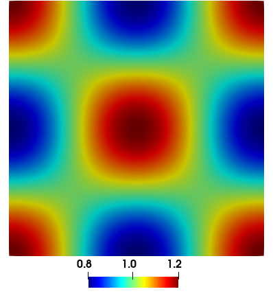
(a) t=0.0

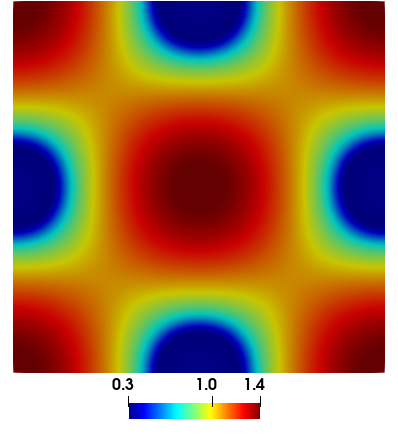
(b) t=0.2

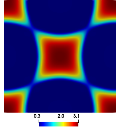
(c) t=0.4

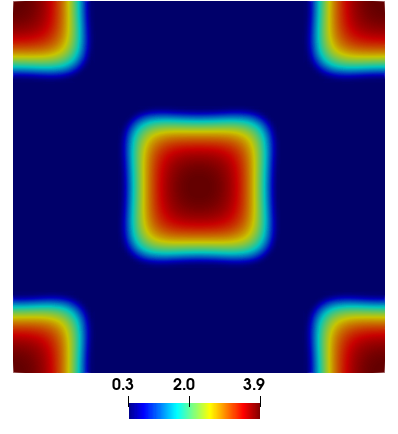
(d) t=0.6

Figure 2: Snapshots of the surface height contour following the thin film equation (1.1) at different times starting from the initial condition (4.1), showing stages in the dewetting of a two-dimensional thin film with weak condensation: (a) initial profile, (b) formation and spreading of dry spots, (c) break-up of ridges, (d) formation of droplets that slowly condense in time.

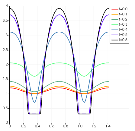
Figure 3: Time evolution of the surface height along the north-east diagonal cutline in Figure 2.

4.2 MFC for droplet dynamics.

Next, we apply the developed finite element discretization and the PDHG algorithm 1 to solve the full MFC system (2) with $\beta>0$. We use the following potential and terminal functionals:

$$\mathcal{F}(h)=-0.02\int_{0}^{T}\int_{\Omega}h\log(h)dx\,dt,\quad\mathcal{G}(h)=0.05\int_{\Omega}h\log(h/h_{\mathrm{trg}})dx,$$

where $h_{\mathrm{trg}}$ is a target terminal surface height. We take the terminal time $T=1$ and $\beta=0.01$. With different choices of initial and target surface heights, we present numerical results showcasing the application of the developed MFC scheme for fundamental droplet actuation techniques, including droplet transport, bead-up (i.e., dewetting), spreading, merging, and splitting.

In the finite element discretization (3.2), we use a uniform spatial rectangular mesh of size $64\times 64$, a uniform temporal mesh of size $16$, and take polynomial degree $k=4$. The same stopping criteria as the previous example is used for the PDHG Algorithm 1.

Case 1: Droplet transport.

Droplet transport is one of the most important operations in digital microfluidics (DMF) and has been extensively investigated through experimental approaches such as electro-dewetting (Li et al., 2019). In Figures 4 - 5, we present the results of the MFC problem (2) with the initial and target surface heights specified as

$$h_{0}(x,y)= \;\epsilon+\frac{10}{3}\left(1-75((x-0.3)^{2}+(y-0.3)^{2})\right)_{+},$$

$$h_{\mathrm{trg}}(x,y)= \;\epsilon+\frac{10}{3}\left(1-75((x-0.7)^{2}+(y-0.7)^{2})\right)_{+}.$$

Here $(f)_{+}=\begin{cases}f&\quad\text{if }f\geq 0,\\[0.86108pt] 0&\quad\text{otherwise}\end{cases}$ is the positive part of a function $f$. This example models the MFC of an initial parabolic droplet centered at $(0.3,0.3)$ moving towards a target parabolic droplet centered at $(0.7,0.7)$. The snapshots in Figure 4 depict that the droplet quickly breaks symmetry, beads up, and develops a larger advancing contact angle, leaving a capillary wave as the droplet advances towards the target position. Meanwhile, the droplet size increases in the early stage and then decreases to the desired droplet height through non-mass-conserving fluxes.

(a) (b)
(c) (d)

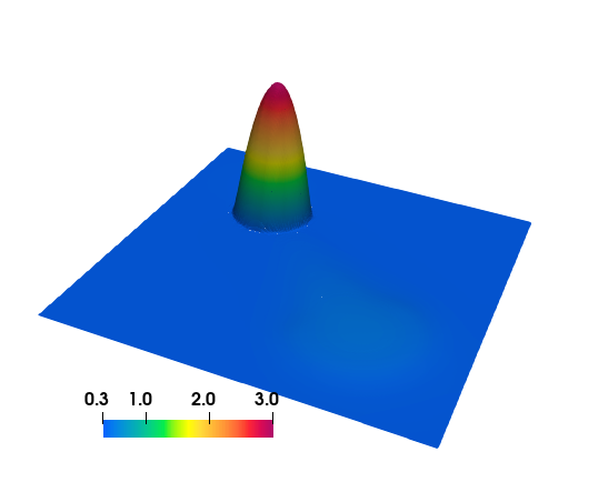
Figure 4: Case 1 (Droplet transport). Snapshots of the controlled surface height contour at different times by solving the MFC problem (2): (a) $t=0.0$, (b) $t=0.3$, (c) $t=0.7$, (d) $t=1.0$.

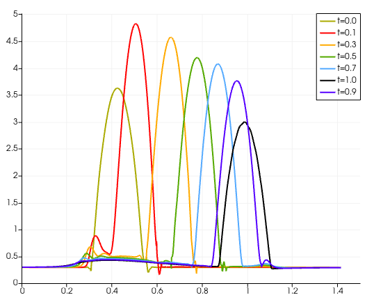
Figure 5: Case 1 (Droplet transport). Time evolution of the controlled surface height along the north-east diagonal cutline for the controlled dynamics in Figure 4.

Case 2: Droplet spreading.

Controlling the deformation of a droplet is also a crucial aspect of liquid-handling technology. For instance, in typical electro-wetting and electro-dewetting experiments, an electric field can induce changes in the contact angles of a slender droplet containing a dilute surfactant (Nelson & Kim, 2012). Here, we demonstrate the MFC mechanism to control the spreading and bead-up of droplets.

For the droplet spreading example, we take the initial and target surface heights as

$$h_{0}(x,y)= \;\epsilon+\frac{10}{3}\left(1-75((x-0.5)^{2}+(y-0.5)^{2})\right)_{+},$$

$$h_{\mathrm{trg}}(x,y)= \;\epsilon+\frac{5}{12}\left(1-\frac{75}{8}((x-0.5)^{2}+(y-0.5)^{2})\right)_{+}.$$

This case models the MFC of an initial parabolic droplet centered at $(0.5,0.5)$ with half-width $w=\frac{1}{5\sqrt{3}}$ flattening towards the target droplet with half-width $w=\frac{2\sqrt{2}}{5\sqrt{3}}$ . The initial and target droplets have the same total mass. Snapshots of the simulation results for the scheme (3.2) are presented in Figures 6 - 7. The numerical results indicate that the controlled droplet initially evolves into a pancake shape and then gradually converges to the target droplet profile over time. The radial symmetry in the droplet profile is preserved during the evolution.

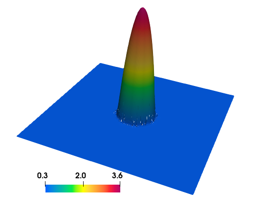
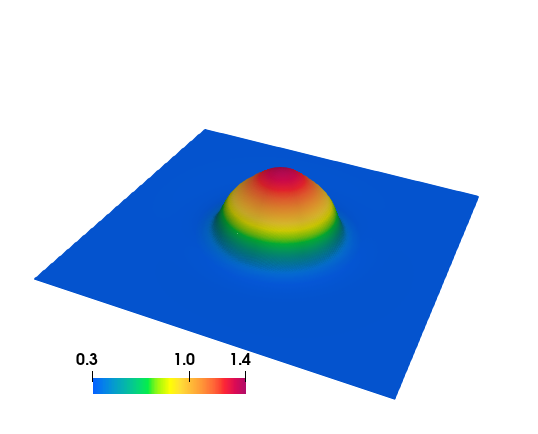
(a) (b)
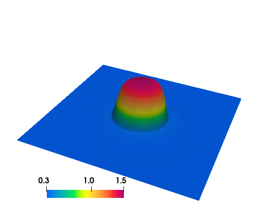
(c) (d)

Figure 6: Case 2 (Droplet spreading). Snapshots of the controlled surface height contour at different times: (a) $t=0.0$, (b) $t=0.3$, (c) $t=0.7$, (d) $t=1.0$.

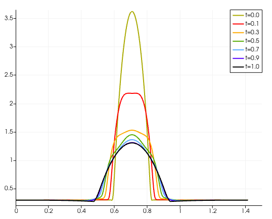
Figure 7: Case 2 (Droplet spreading). Dynamic evolution of the controlled surface height along the north-east diagonal cutline shown in Figure 6.

Case 3: Droplet bead-up.

This represents the reverse process of Case 2, where our objective is to induce droplet bead-up (i.e. dewetting). Therefore, we set the initial and target surface heights as

$$h_{0}(x,y)= \;\epsilon+\frac{5}{12}\left(1-\frac{75}{8}((x-0.5)^{2}+(y-0.5)^{2})\right)_{+},$$

$$h_{\mathrm{trg}}(x,y)= \;\epsilon+\frac{10}{3}\left(1-75((x-0.5)^{2}+(y-0.5)^{2})\right)_{+},$$

where the initial and target profiles are reversed compared to the example in Case 2. This models the MFC of an initial parabolic droplet centered at $(0.5,0.5)$ with half-width $w=\frac{2\sqrt{2}}{5\sqrt{3}}$ which beads up and evolves into the target droplet with half-width $w=\frac{1}{5\sqrt{3}}$. Snapshots of the simulation results for the scheme (3.2) are presented in Figures 8 - 9. In this case, we observe more pattern formation during the droplet bead-up process, where capillary waves are generated in the early stage before the droplet reaches the target shape. Compared to the target droplet profile, the obtained profile at the terminal time $t=1$ has a slightly elevated height near the contact line.

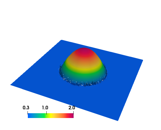
(a) (b)
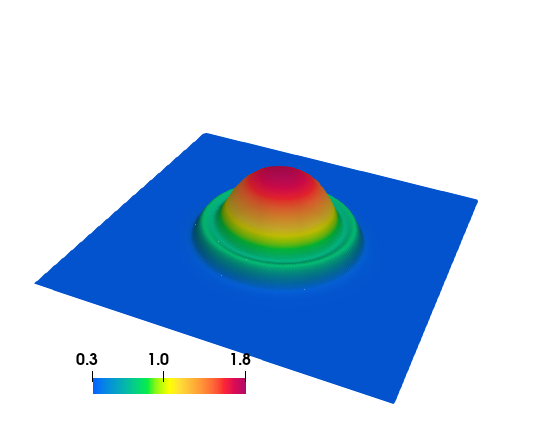
(c) (d)

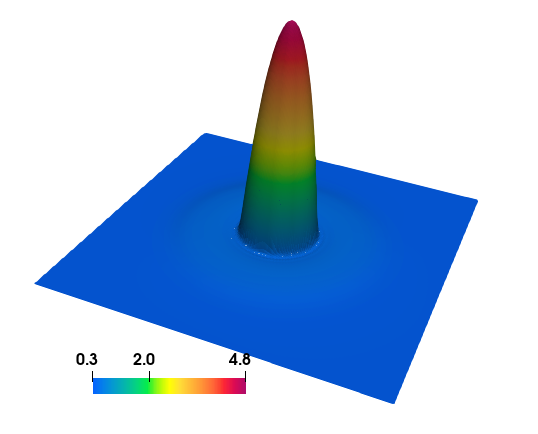
Figure 8: Case 3 (Droplet bead-up). Snapshots of the controlled surface height contour at different times: (a) $t=0.0$, (b) $t=0.3$, (c) $t=0.7$, (d) $t=1.0$.

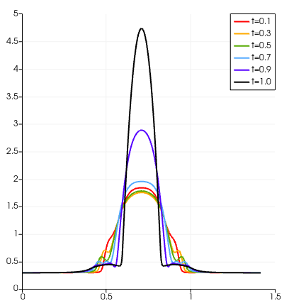
Figure 9: Case 3 (Droplet bead-up). Time evolution of the controlled surface height along the north-east diagonal cutline shown in Figure 8.

Case 4: Droplet merging.

Finally, we demonstrate the application of MFC for droplet merging and splitting, which are more complex droplet manipulation techniques widely used in biological and chemical applications (Nan et al., 2023). For the droplet merging case, we control the coalescence of four small droplets initially placed on a two-dimensional domain, where the initial and target surface height profiles are set as

$$h_{0}(x,y)= \;\epsilon+\sum_{i=1}^{4}\tfrac{5}{6}[1-75((x-x_{i})^{2}+(y-y_{i})^{2})]_{+},$$

$$h_{\mathrm{trg}}(x,y)= \;\epsilon+\tfrac{5}{12}[1-\tfrac{75}{8}((x-0.5)^{2}+(y-0.5)^{2})]_{+},$$

where the positions of the peaks of the initial droplets are $(x_{1},y_{1})=(0.3,0.3)$, $(x_{2},y_{2})=(0.3,0.7)$, $(x_{3},y_{3})=(0.7,0.3)$, and $(x_{4},y_{4})=(0.7,0.7)$. Snapshots of the simulation results using the scheme (3.2) for this case are presented in Figure 10 - 11. Similar to the droplet transport example discussed in Case 1, the controlled droplets quickly bead up and start moving toward the center of the domain, where the target droplet is placed. Capillary waves are created behind the droplets as they shift towards the target position. Near the terminal time $t=1$, the droplet coalescence occurs, forming a single droplet at the center of the domain.

(a) (b)
(c) (d)

Figure 10: Case 4 (Droplet merging). Snapshots of the controlled surface height contour at different times: (a) $t=0.0$, (b) $t=0.3$, (c) $t=0.7$, (d) $t=1.0$.

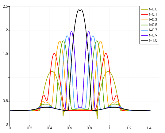
Figure 11: Case 4 (Droplet merging). Time evolution of the controlled surface height along the north-east diagonal cutline shown in Figure 10.

Case 5: Droplet splitting.

For the case of droplet splitting, we consider the reverse process of the droplet merging considered in Case 4 and take the initial and target surface heights as

$$h_{0}(x,y)= \;\epsilon+\tfrac{5}{12}[1-\tfrac{75}{8}((x-0.5)^{2}+(y-0.5)^{2})]_{+},$$

$$h_{\mathrm{trg}}(x,y)= \;\epsilon+\sum_{i=1}^{4}\tfrac{5}{6}[1-75((x-x_{i})^{2}+(y-y_{i})^{2})]_{+},$$

where the initial and target profiles are reversed compared to the example in Case 4, and the locations of the peaks $\{(x_{i},y_{i})\}$ in the target profile are identical to those in the initial profile specified in Case 4. Snapshots of the simulation results for the controlled dynamics using the scheme (3.2) are presented in Figures 12 - 13. This example models the MFC of one initial parabolic droplet splitting into four smaller droplets and shifting into target positions individually. Compared to the droplet merging case, splitting a single droplet appears to be more challenging, and the terminal surface height profile obtained at the terminal time $t=1$ still maintains a ridge connecting the small droplets.

(a) (b)
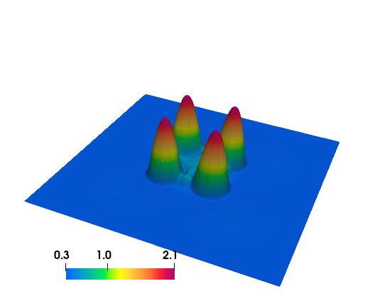
(c) (d)

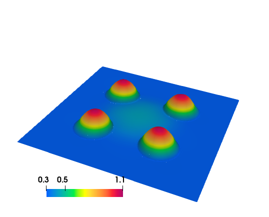
Figure 12: Case 5 (Droplet splitting). Snapshots of the controlled surface height contour at different times. (a) $t=0.0$, (b) $t=0.3$, (c) $t=0.7$, (d) $t=1.0$.

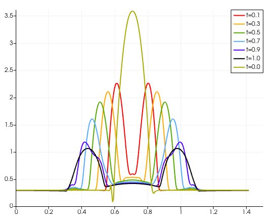
Figure 13: Case 5 (Droplet splitting). Time evolution of the controlled surface height along the north-east diagonal cutline shown in Figure 12.

5 Discussions

In this paper, we formulate and numerically compute mean field control problems for droplet dynamics governed by a thin film equation with a non-mass-conserving flux. Our formulation starts with droplet dynamics, which are gradient flows of free energies in optimal transport metric spaces with nonlinear mobility functions. We design and compute these mean field control problems of droplet dynamics using the primal-dual hybrid gradient algorithms with high-order finite element approximation schemes. Numerical examples of two-dimensional uncontrolled and controlled droplet dynamics demonstrate the effectiveness of the proposed control mechanisms.

The proposed mean field control problems open the door to studying experimental design problems of droplet dynamics. Typical questions include the general choice of free energies and mobility functions in modeling droplet pattern formulations. For example, one may design suitable free energies coupled with other external field constraints to adapt our proposed mean field control approach for controlling droplet dynamics via temperature (Ji et al., 2021) or electric fields (Chu et al., 2023; Eaker & Dickey, 2016). In simulations, one of the challenges is the nonconvex formulations of general mean field variational problems in controlling the dynamical behaviors of droplets. Suitable regularization functionals are needed to maintain the stability of simulations. We leave these studies for future work.

Declaration of Interests

The authors report no conflict of interest.

Appendix A

In the appendix, we prove the Proposition 2.1.

Proof A.12 (Proof of Proposition 2.1).

Denote the Lagrange multiplier of the MFC problem (2.9) as $\phi\colon[0,T]\times\Omega\rightarrow\mathbb{R}$. Consider the following saddle point problem:

$$\begin{split}\inf_{\bm{m},s,h,h_{T}}\sup_{\phi}\quad\mathcal{L}(\bm{m},s,h,h_{T},\phi),\end{split}$$

where

$$\begin{split}\mathcal{L}(\bm{m},s,h,h_{T},\phi)=&\int_{0}^{T}\int_{\Omega}\Big{[}\frac{\|\bm{m}\|^{2}}{2V_{1}(h)}+\frac{|s|^{2}}{2V_{2}(h)}+\phi\Big{(}\partial_{t}h+\nabla\cdot\bm{m}-s\Big{)}\Big{]}dxdt\\ &+\int_{0}^{T}\Big{[}\frac{\beta^{2}}{2}\mathcal{I}(h)-\mathcal{F}(h)\Big{]}dt+\mathcal{G}(h_{T})+\beta\mathcal{E}(h_{T}).\end{split}$$

Assume $h>0$. By solving the saddle point problem of $\mathcal{L}$, i.e., taking the $L^{2}$ first variation of $\mathcal{L}$ on variables $\bm{m}$, $s$, $h$, $h_{T}$, we derive

$$\left\{\begin{split}&\frac{\delta}{\delta\bm{m}}\mathcal{L}=0,\\ &\frac{\delta}{\delta s}\mathcal{L}=0,\\ &\frac{\delta}{\delta h}\mathcal{L}=0,\\ &\frac{\delta}{\delta\phi}\mathcal{L}=0,\\ &\frac{\delta}{\delta h_{T}}\mathcal{L}=0,\\ \end{split}\right.\quad\Rightarrow\quad\left\{\begin{split}&\frac{\bm{m}}{V_{1}}=\nabla\phi,\\ &\frac{s}{V_{2}}=\phi,\\ &-\frac{1}{2}\frac{\|\bm{m}\|^{2}}{V_{1}^{2}}V_{1}^{\prime}-\frac{1}{2}\frac{|s|^{2}}{V_{2}^{2}}V_{2}^{\prime}+\frac{\delta}{\delta h}\Big{[}\frac{\beta^{2}}{2}\mathcal{I}(h)-\mathcal{F}(h)\Big{]}-\partial_{t}\phi=0,\\ &\partial_{t}h+\nabla\cdot\bm{m}-s=0,\\ &\phi_{T}+\frac{\delta}{\delta h_{T}}\Big{(}\mathcal{G}(h_{T})+\beta\mathcal{E}(h_{T})\Big{)}=0.\end{split}\right.$$

We finish the derivation of the mean field control system.

We next derive the $L^{2}$ first variation of the Fisher information functional $\mathcal{I}$. Recall

$$\mathcal{I}(h)=\frac{1}{2}\int_{\Omega}\left(V_{1}(h)|\nabla P(h)|^{2}+V_{2}(h)|P(h)|^{2}\right)dx,$$

where $P(h)=\Pi(h)-\mathcal{P}_{*}-\alpha^{2}{\Delta h}$, with the notation $\Delta h=\nabla^{2}h$. Consider a smooth test function $\delta h\in C^{\infty}([0,T];\mathbb{R})$. Then

$$\begin{split}&\mathcal{I}(h+\epsilon\delta h)\\ =&\frac{1}{2}\int_{\Omega}\left(V_{1}(h+\epsilon\delta h)|\nabla P(h+\epsilon\delta h)|^{2}+V_{2}(h+\epsilon\delta h)|P(h+\epsilon\delta h)|^{2}\right)dx\\ =&\quad\frac{1}{2}\int_{\Omega}(V_{1}(h)+\epsilon V_{1}^{\prime}(h)\delta h)|\nabla P(h)+\epsilon\nabla(\Pi^{\prime}(h)\delta h-\alpha^{2}\Delta\delta h)|^{2}dx\\ &+\frac{1}{2}\int_{\Omega}(V_{2}(h)+\epsilon V_{2}^{\prime}(h)\delta h)|P(h)+\epsilon(\Pi^{\prime}(h)\delta h-\alpha^{2}\Delta\delta h)|^{2}dx+O(\epsilon^{2})\\ =&\mathcal{I}(h)+\epsilon\int_{\Omega}\left(\frac{1}{2}V_{1}^{\prime}(h)\delta h|\nabla P(h)|^{2}+V_{1}(h)\nabla P(h)\cdot\nabla(\Pi^{\prime}(h)\delta h-\alpha^{2}\Delta\delta h)\right)dx\\ &\qquad+\epsilon\int_{\Omega}\left(\frac{1}{2}V_{2}^{\prime}(h)\delta h|P(h)|^{2}+V_{2}(h)P(h)(\Pi^{\prime}(h)\delta h-\alpha^{2}\Delta\delta h)\right)dx+O(\epsilon^{2}),\end{split}$$

where $O(\epsilon^{2})$ is the asymptotic notation. Using the definition of $L^{2}$ first variation operator,

$$\mathcal{I}(h+\epsilon\delta h)-\mathcal{I}(h)=\epsilon\int_{\Omega}\frac{\delta}{\delta h}\mathcal{I}(h)\delta hdx+O(\epsilon^{2}),$$

and applying the integration by parts, we derive the $L^{2}$ first variation of functional $\mathcal{I}$.

References

- Ajaev (2005) Ajaev, V. S. 2005 Spreading of thin volatile liquid droplets on uniformly heated surfaces. Journal of Fluid Mechanics 528, 279–296.
- Ajaev & Homsy (2001) Ajaev, V. S. & Homsy, G. M. 2001 Steady vapor bubbles in rectangular microchannels. Journal of Colloid and Interface Science 240 (1), 259–271.
- Al Jamal & Morris (2018) Al Jamal, Rasha & Morris, Kirsten 2018 Linearized stability of partial differential equations with application to stabilization of the kuramoto–sivashinsky equation. SIAM Journal on Control and Optimization 56 (1), 120–147.
- Anderson et al. (2021) Anderson, Robert, Andrej, Julian, Barker, Andrew & et al. 2021 MFEM: A modular finite element methods library. Comput. Math. Appl. 81, 42–74.
- Armaou & Christofides (2000) Armaou, Antonios & Christofides, Panagiotis D 2000 Feedback control of the kuramoto–sivashinsky equation. Physica D: Nonlinear Phenomena 137 (1-2), 49–61.
- Benamou & Brenier (2000) Benamou, Jean-David & Brenier, Yann 2000 A computational fluid mechanics solution to the monge-kantorovich mass transfer problem. Numerische Mathematik 84 (3), 375–393.
- Bertozzi et al. (2001) Bertozzi, A. L., Grün, G. & Witelski, T. P. 2001 Dewetting films: bifurcations and concentrations. Nonlinearity 14 (6), 1569.
- Biswal et al. (2024) Biswal, Shiba, Ji, Hangjie, Elamvazhuthi, Karthik & Bertozzi, Andrea L. 2024 Optimal boundary control of a model thin-film fiber coating model. Physica D: Nonlinear Phenomena 457, 133942.
- Boffi et al. (2013) Boffi, Daniele, Brezzi, Franco & Fortin, Michel 2013 Mixed finite element methods and applications, Springer Series in Computational Mathematics, vol. 44. Springer, Heidelberg.
- Carrillo et al. (2022) Carrillo, José A., Craig, Katy, Wang, Li & Wei, Chaozhen 2022 Primal dual methods for Wasserstein gradient flows. Found. Comput. Math. 22 (2), 389–443.
- Carrillo et al. (2023) Carrillo, Jose A., Wang, Li & Wei, Chaozhen 2023 Structure preserving primal dual methods for gradient flows with nonlinear mobility transport distances .
- Chambolle & Pock (2011) Chambolle, Antonin & Pock, Thomas 2011 A first-order primal-dual algorithm for convex problems with applications to imaging. J. Math. Imaging Vision 40 (1), 120–145.
- Christofides & Armaou (2000) Christofides, Panagiotis D & Armaou, Antonios 2000 Global stabilization of the kuramoto–sivashinsky equation via distributed output feedback control. Systems & Control Letters 39 (4), 283–294.
- Chu et al. (2023) Chu, Weiqi, Ji, Hangjie, Wang, Qining, Kim, Chang-Jin “CJ”, Bertozzi, Andrea L & others 2023 Electrohydrodynamics modeling of droplet actuation on a solid surface by surfactant-mediated electrodewetting. Physical Review Fluids 8 (7), 073701.
- Cimpeanu et al. (2021) Cimpeanu, Radu, Gomes, Susana N & Papageorgiou, Demetrios T 2021 Active control of liquid film flows: beyond reduced-order models. Nonlinear Dynamics 104 (1), 267–287.
- Coron & Lü (2015) Coron, Jean-Michel & Lü, Qi 2015 Fredholm transform and local rapid stabilization for a kuramoto–sivashinsky equation. Journal of Differential Equations 259 (8), 3683–3729.
- Eaker & Dickey (2016) Eaker, Collin B & Dickey, Michael D 2016 Liquid metal actuation by electrical control of interfacial tension. Applied Physics Reviews 3 (3).
- Fu et al. (2023a) Fu, Guosheng, Osher, Stanley & Li, Wuchen 2023a High order spatial discretization for variational time implicit schemes: Wasserstein gradient flows and reaction-diffusion systems. arXiv:2303.08950 [math.NA] .
- Fu et al. (2023b) Fu, Guosheng, Osher, Stanley, Pazner, Will & Li, Wuchen 2023b Generalized optimal transport and mean field control problems for reaction-diffusion systems with high-order finite element computation. arXiv preprint arXiv:2306.06287 .
- Gao & Qi (2024) Gao, Yuan & Qi, Di 2024 Mean field games for controlling coherent structures in nonlinear fluid systems. arXiv preprint arXiv:2401.10356 .
- Glasner & Witelski (2003) Glasner, K. B. & Witelski, T. P. 2003 Coarsening dynamics of dewetting films. Physical Review E 67 (1), 016302.
- Jacobs et al. (2019) Jacobs, Matt, Léger, Flavien, Li, Wuchen & Osher, Stanley 2019 Solving large-scale optimization problems with a convergence rate independent of grid size. SIAM Journal on Numerical Analysis 57 (3), 1100–1123.
- Ji et al. (2021) Ji, Hangjie, Falcon, Claudia, Sedighi, Erfan, Sadeghpour, Abolfazl, Ju, Y Sungtaek & Bertozzi, Andrea L 2021 Thermally-driven coalescence in thin liquid film flowing down a fibre. Journal of Fluid Mechanics 916, A19.
- Ji & Witelski (2018) Ji, H. & Witelski, T. P. 2018 Instability and dynamics of volatile thin films. Physical Review Fluids 3 (2), 024001.
- Jiang et al. (2022) Jiang, Youhua, Feng, Leyun, O’Donnell, Allison, Machado, Christian, Choi, Wonjae, Patankar, Neelesh A. & Park, Kyoo-Chul 2022 Coalescence-induced propulsion of droplets on a superhydrophilic wire. Applied Physics Letters 121 (23), 231602, arXiv: https://pubs.aip.org/aip/apl/article-pdf/doi/10.1063/5.0124560/16486293/231602_1_online.pdf.
- Jordan et al. (1998) Jordan, Richard, Kinderlehrer, David & Otto, Felix 1998 The variational formulation of the fokker–planck equation. SIAM Journal on Mathematical Analysis 29 (1), 1–17, arXiv: https://doi.org/10.1137/S0036141096303359.
- Katz & Fridman (2020) Katz, Rami & Fridman, Emilia 2020 Finite-dimensional control of the kuramoto-sivashinsky equation under point measurement and actuation. In 2020 59th IEEE Conference on Decision and Control (CDC), pp. 4423–4428. IEEE.
- Khoshmanesh et al. (2017) Khoshmanesh, Khashayar, Tang, Shi-Yang, Zhu, Jiu Yang, Schaefer, Samira, Mitchell, Arnan, Kalantar-Zadeh, Kourosh & Dickey, Michael D 2017 Liquid metal enabled microfluidics. Lab on a Chip 17 (6), 974–993.
- Kim (2001) Kim, Chang-Jin “CJ” 2001 Micropumping by electrowetting. In ASME international mechanical engineering congress and exposition, , vol. 35593, pp. 55–62. American Society of Mechanical Engineers.
- Klein & Prohl (2016) Klein, Markus & Prohl, Andreas 2016 Optimal control for the thin film equation: Convergence of a multi-parameter approach to track state constraints avoiding degeneracies. Computational Methods in Applied Mathematics 16 (4), 685–702.
- Lee & Tran (2005) Lee, CH & Tran, HT 2005 Reduced-order-based feedback control of the kuramoto–sivashinsky equation. Journal of computational and applied mathematics 173 (1), 1–19.
- Li et al. (2019) Li, Jia, Ha, Noel S, Liu, Tingyi ‘Leo’, van Dam, R Michael & ‘CJ’ Kim, Chang-Jin 2019 Ionic-surfactant-mediated electro-dewetting for digital microfluidics. Nature 572 (7770), 507–510.
- Li et al. (2022a) Li, Wuchen, Lee, Wonjun & Osher, Stanley 2022a Computational mean-field information dynamics associated with reaction-diffusion equations. J. Comput. Phys. 466, Paper No. 111409, 30.
- Li et al. (2022b) Li, Wuchen, Liu, Siting & Osher, Stanley 2022b Controlling conservation laws ii: Compressible navier–stokes equations. Journal of Computational Physics 463, 111264.
- Li et al. (2023) Li, Wuchen, Liu, Siting & Osher, Stanley 2023 Controlling conservation laws i: entropy-entropy flux. Journal of Computational Physics 480.
- Li et al. (2020) Li, Wuchen, Lu, Jianfeng & Wang, Li 2020 Fisher information regularization schemes for Wasserstein gradient flows. J. Comput. Phys. 416, 109449, 24.
- Liu & Krstić (2001) Liu, Wei-Jiu & Krstić, Miroslav 2001 Stability enhancement by boundary control in the kuramoto–sivashinsky equation. Nonlinear Analysis: Theory, Methods & Applications 43 (4), 485–507.
- Maghenem et al. (2022) Maghenem, Mohamed, Prieur, Christophe & Witrant, Emmanuel 2022 Boundary control of the kuramoto-sivashinsky equation under intermittent data availability. In American Control Conference.
- Mielke (2011) Mielke, Alexander 2011 A gradient structure for reaction-diffusion systems and for energy-drift-diffusion systems. Nonlinearity 24 (4), 1329–1346.
- Nan et al. (2023) Nan, Lang, Mao, Tianjiao & Shum, Ho Cheung 2023 Self-synchronization of reinjected droplets for high-efficiency droplet pairing and merging. Microsystems & Nanoengineering 9 (1), 24.
- Nelson & Kim (2012) Nelson, Wyatt C & Kim, Chang-Jin ‘CJ’ 2012 Droplet actuation by electrowetting-on-dielectric (ewod): A review. Journal of Adhesion Science and Technology 26 (12-17), 1747–1771.
- Oron & Bankoff (2001) Oron, A. & Bankoff, S. G. 2001 Dynamics of a condensing liquid film under conjoining/disjoining pressures. Physics of Fluids 13 (5), 1107–1117.
- Oron et al. (1997) Oron, A., Davis, S. H. & Bankoff, S. G. 1997 Long-scale evolution of thin liquid films. Reviews of Modern Physics 69 (3), 931.
- Pazner et al. (2023) Pazner, Will, Kolev, Tzanio & Dohrmann, Clark R. 2023 Low-order preconditioning for the high-order finite element de Rham complex. SIAM J. Sci. Comput. 45 (2), A675–A702.
- Sadeghpour et al. (2021) Sadeghpour, A., Oroumiyeh, F., Zhu, Y., Ko, D. D., Ji, H., Bertozzi, A. L. & Ju, Y. S. 2021 Experimental study of a string-based counterflow wet electrostatic precipitator for collection of fine and ultrafine particles. Journal of the Air & Waste Management Association pp. 1–15.
- Sadeghpour et al. (2019) Sadeghpour, A, Zeng, Z, Ji, H, Ebrahimi, N Dehdari, Bertozzi, AL & Ju, YS 2019 Water vapor capturing using an array of traveling liquid beads for desalination and water treatment. Science Advances 5 (4), eaav7662.
- Samoilova & Nepomnyashchy (2019) Samoilova, Anna E & Nepomnyashchy, Alexander 2019 Feedback control of marangoni convection in a thin film heated from below. Journal of Fluid Mechanics 876, 573–590.
- Shankar et al. (2022) Shankar, Suraj, Raju, Vidya & Mahadevan, L 2022 Optimal transport and control of active drops. Proceedings of the National Academy of Sciences 119 (35), e2121985119.
- Thiele et al. (2016) Thiele, Uwe, Archer, Andrew J & Pismen, Len M 2016 Gradient dynamics models for liquid films with soluble surfactant. Physical Review Fluids 1 (8), 083903.
- Tomlin et al. (2019) Tomlin, Ruben J, Gomes, Susana N, Pavliotis, Grigorios A & Papageorgiou, Demetrios T 2019 Optimal control of thin liquid films and transverse mode effects. SIAM Journal on Applied Dynamical Systems 18 (1), 117–149.
- Villani (2008) Villani, Cédric 2008 Optimal transport: old and new, , vol. 338. Springer Science & Business Media.
- Wray et al. (2022) Wray, Alexander W, Cimpeanu, Radu & Gomes, Susana N 2022 Electrostatic control of the navier-stokes equations for thin films. Physical Review Fluids 7 (12), L122001.