GenEFT: Understanding Statics and Dynamics of Model Generalization via Effective Theory

Abstract

We present GenEFT: an effective theory framework for shedding light on the statics and dynamics of neural network generalization, and illustrate it with graph learning examples. We first investigate the generalization phase transition as data size increases, comparing experimental results with information-theory-based approximations. We find generalization in a Goldilocks zone where the decoder is neither too weak nor too powerful. We then introduce an effective theory for the dynamics of representation learning, where latent-space representations are modeled as interacting particles (“repons”), and find that it explains our experimentally observed phase transition between generalization and overfitting as encoder and decoder learning rates are scanned. This highlights the power of physics-inspired effective theories for bridging the gap between theoretical predictions and practice in machine learning.

1 Introduction

A key feature if intelligence is the ability to generalize, exploiting patterns seen in data to improve predictions for unseen data. There is therefore great interest in how to choose datasets and model hyperparameters that lead to generalization as opposed to overfitting, to which state-of-the-art machine learning models with high complexity are often prone  (Bejani & Ghatee, 2021). The machine learning community has traditionally made such choices on a case-by-case basis, without a unifying effective theory that provides a systematic recipe for designing the generalizable model. In this paper, we take a modest step toward such a theory by presenting GenEFT: a unifying effective theory framework for understanding model generalization in practice. Specifically, we aim to answer the following three questions:

Q1: Critical data size – Given a problem, how large a dataset is needed for the model to be generalizable?

Q2: Optimal model complexity – How does model complexity affect generalization?

Q3: Critical learning rate – How do the learning rates affect generalization?

We provide theoretical frameworks and empirical evidence to shed light on these questions. In summary, our conclusions are as follows:

A1: We present an information-theoretic approximation that describes the relationship between test accuracy and the amount of fraction of training data. For graph learning, full generalization only becomes possible after training on at least $b$ examples, where $b=\log_{2}N$ is the number of bits required to specify which of $N$ possible graphs is present, and further delays are caused both by correlated data and by the induction gap, bits required to learn the inductive biases (graph properties) that enable generalization.

A2: Generalization occurs in the complexity Goldilocks zone where it is capable enough to exploit a clever representation, but still incapable of memorizing the training data.

A3: We successfully predict how the memorization/generalization phase transition depends on encoder and decoder learning rates by modeling the representations as interacting particles that we term “repons”.

In summary, we conclude that (a) static/steady state properties of generalization, such as the critical training fraction and optimal model complexity, could be derived from information-theoretic properties of the input, and (b) dynamic properties of generalization, such as critical learning rate, could be derived from studying the system of interacting repons, particles whose locations are given by their embedding representations. This framework is summarized in Figure 1.

The rest of this paper is organized as follows: In Section 2, we formally describe our problem settings. In the following three sections, Section 3–5, we tackle the three questions Q1, Q2, Q3, respectively, using a combination of theoretical frameworks and empirical evidence. We discuss related work in Section 6, and summarize our conclusions in Section 7.

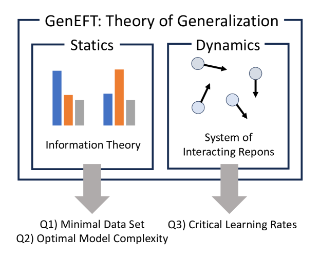
Figure 1: A unifying framework for understanding generalization.

2 Problem Formulation

Consider an arbitrary binary relation $R$ of elements $x_{1},...,x_{n}$, for example “greater-than” or “equal modulo 3”. This can be equivalently viewed as a directed graph of order $n$, and is specified by the $n\times n$ matrix $\textbf{R}_{ij}\equiv R(x_{i},x_{j})\in\{0,1\}$. Our machine-learning task is to predict the probability that $R(x_{i},x_{j})=1$ by training on a random data subset.

Model Architecture: We use an encoder-decoder architecture where the encoder maps each input $x$ into a latent space representation $\mathbf{E}_{x}\in\mathbb{R}^{d}$ after which an MLP decoder concatenates two embeddings $[\mathbf{E}_{x_{1}},\mathbf{E}_{x_{2}}]$ and maps it into the probability estimate. We use $\tanh$ activation in any hidden layers followed by a sigmoid function to obtain the probability. The learnable parameters in the model are the embedding vectors and well as the weights and biases in the decoder MLP.

Datasets The relations $R$ that were used in our experiments are equal modulo 3, equal modulo 5, greater-than, and complete bipartite graph, whose formal definitions are summarized in Table 1. These relations were chosen to provide a broad diversity of relation properties. For instance, equal modulo 3 and equal modulo 5 are equivalence classes (symmetric, reflexive, and transitive), greater-than is total ordering (antisymmetric and transitive), while the complete bipartite graph is symmetric and anti-transitive. We will see that our effective theory is applicable to these general relations regardless of their detailed properties. We used $n=30$ elements for our experiments. For each relation, we thus have $n^{2}=900$ data samples $\textbf{R}_{ij}$. The training data was randomly sampled from this set, and the remaining samples were used for validation (testing).

Table 1: Relations used in the experiments. $S$ is one of two disjoint sets in a bipartite graph.

Relation	Description
Modulo $3$	$(x,y)\in R$ iff $x\equiv y\;(\textrm{mod}\;3)$
Modulo $5$	$(x,y)\in R$ iff $x\equiv y\;(\textrm{mod}\;5)$
Greater-than	$(x,y)\in R$ iff $x<y$
Complete Bipartite Graph $G=(S,\overline{S})$	$(x,y)\in R$ iff ($x\in S,y\notin S$) or ($x\notin S$, $y\in S$)

3 Minimal Data Amount for Generalization

Table 2: Bits required to describe relations with various properties.

Relation	Description length $b$ [bits]
Generic	$n^{2}$
Symmetric	$n(n+1)/2$
Antisymmetric	$n(n+1)/2$
Reflexive	$n(n-1)$
Transitive	$\approx\frac{n^{2}}{(\langle k\rangle-1)!}$, $\langle k\rangle$ is the average length of a transitive chain
Equivalence Relation with $k$ Classes	$\approx n\log_{2}k$
Total Ordering	$\log_{2}n!\approx n\textrm{log}_{2}{n\over 2}$
Complete Bipartite Graph	$n$
Incomplete Bipartite Graph $G=(S_{1},S_{2})$	$|S_{1}||S_{2}|$
Tree Graph	$\approx n\textrm{log}_{2}\langle d\rangle$ where $\langle d\rangle$ is the average node depth

Effective Theory: Information-theoretic Approach:

Let $b$ be the relation’s description length, i.e., the minimum number of independent bits required to fully describe it. For graphs sampled uniformly from a class with certain properties (transitivity and symmetry, say), $b=\log_{2}C$, where $C$ is the total number of graphs satisfying these properties. For instance, there are $n!$ total orderings, giving $b\approx n\log_{2}(n/2)$ using Stirling’s approximation.

To fully generalize and figure out precisely which graph in its class we are dealing with, we therefore need at least $b$ training data samples, since they provide at most one bit of information each. As seen in Figures 2 and 3, $b$ indeed sets the approximate scale for how many training data samples are needed to generalize, but to generalize perfectly, we need more than this strict minimum for two separate reasons.

1. $k$ data samples may provide less than $k$ bits of information because (a) they are unbalanced (giving 0 and 1 with unequal probability) and (b) they are not independent, with some inferable from others: for example, the data point $R(x_{1},x_{2})$ for a symmetric relation implies that $R(x_{2},x_{1})=1$.

2. We lack a priori knowledge of the inductive bias (what specific properties the graph has), and need to expend some training data information to learn this – we call these extra bits the inductive gap.

Figure 2 shows the theoretical maximum accuracy attainable, computed in two steps. (a) First, we count the total number of directly inferable data pairs using a priori knowledge of the relation – for example, symmetry reflexivity, and transitivity for equivalence relations – given the randomly sampled set of training data pairs. (b) Second, we compute the probability $p_{*}$ of guessing correctly for each case that is not directly inferable from the training data. We do this via Monte Carlo simulation, considering all possible equivalence class memberships (or all possible orderings for the greater-than relation) that are compatible with the training data. The plotted numerical prediction accuracy is a sum of 1 for each inferred relation and ${\rm max}(p_{*},1-p_{*})$ for each non-inferred one, all divided by the total number of examples.

We also provide a simple but useful approximation for how much training data is needed to read a testing accuracy $\alpha$ (say 90%). Let the $b$ bits that describe the relation be $x_{1},x_{2},\cdots x_{b}$, and the number of training data samples is $m$. In the crude approximation that each data sample provides one bit worth of information, this is essentially the problem of putting $m$ distinguishable balls into $b$ different buckets, and we want at least a fraction $\alpha$ of the buckets to be non-empty. The ball that is thrown into an already non-empty bucket does not provide extra information about the relation and therefore, does not affect the prediction accuracy. We use the indicator variable $Z_{i}$: $Z_{i}=1$ iff the bucket $x_{i}$ is empty, $Z_{i}=0$ otherwise. Using the linearity of expectations,

$$E\left(\sum_{i}Z_{i}\right)=\sum_{i}E(Z_{i})=b\left(1-\frac{1}{b}\right)^{m}\;\rightarrow\;E\left(\sum_{i}(1-Z_{i})\right)=b\left[1-\left(1-\frac{1}{b}\right)^{m}\right].$$ (1)

The fraction of inferable data is hence

$$f(m)\approx\frac{1}{b}E\left(\sum_{i}(1-Z_{i})\right)=\left[1-\left(1-\frac{1}{b}\right)^{m}\right].$$ (2)

The critical training data fraction $p_{c}$ is given by $f(Np_{c})=\alpha$, where $N=n^{2}$ is the total number of training samples. This gives the following formula for critical training data fraction:

$$p_{c}=\frac{1}{N}\frac{\textrm{log}_{2}(1-\alpha)}{\textrm{log}_{2}\left(1-\frac{1}{b}\right)},$$ (3)

where the only dependence on the properties of the relation is through its description length $b$. In addition to directly inferable samples using a priori knowledge of the relation, one can also guess the answer and get it correct. Letting $p_{*}$ denote the probability of guessing correctly, the approximation Eq. (2) gives the prediction accuracy

$$f_{\rm UB}(m)=f(m)+\textrm{max}(p_{*},1-p_{*})(1-f(m)),.$$ (4)

For an equivalence relation with $k$ classes, $p_{*}=1/k$. For a complete bipartite graph, $p_{*}=1/2$, since there are only two clusters that each element can belong to. For the greater-than relation, $p_{*}\approx 1/3$. In order to understand this, consider a unit module consisting of three symbols $\{x,y,z\}$, and we are given $x<y$. The only three possible orderings of the three symbols are: $x<y<z$, $x<z<y$, and $z<x<y$. Since each of these orderings are equally likely to be the actual ordering, the probability of correctly guessing the pair $(x,z)$ or $(y,z)$ is $p_{*}=1/3$. We also numerically validate this in Figure 2.

The dashed and solid curves in Figure 2 show rough agreement between this approximation and the more exact Monte Carlo calculation for the inferrable data fraction. One difference is that the training data include a certain level of information also about the pairs that are not directly inferable, improving the aforementioned accuracy term $p_{*}$. Another difference is that data samples on average contain less than one bit (because they are not independent), and that some samples contain more information than others. For example, consider the task of learning greater-than relation on the numbers $0$ to $9$. The sample $0<9$ never provides any extra information, whereas the sample $4<5$ could be powerful if we already know the order of numbers $0$ to $4$ – the comparison of at least 4 additional pairs, $(0,5),(1,5),(2,5),(3,5)$ can then be inferred.

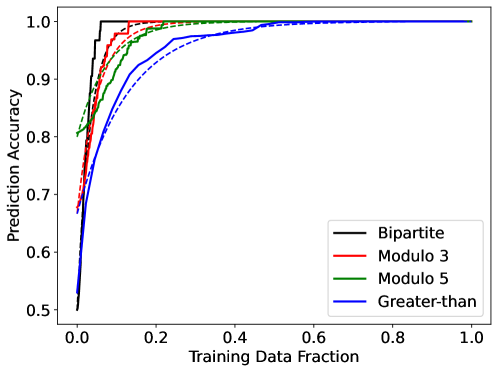
Figure 2: Plot of numerical experiments (solid line) and analytic formula in Eq. 2 (dotted line) for the theoretical upper bound of prediction accuracy $f_{\rm UB}$ as a function of training data fraction.

Figure 2 compares our numerical experiments (solid line) with our analytic approximation (dotted line, Eq. (4)).

Neural Network Experiments:

Figure 3 shows the empirical results of prediction accuracy vs. training data fraction for our neural network experiments. For direct comparison with our theoretical curves, prediction accuracy was computed over the entire dataset, including both the training data and the testing data.

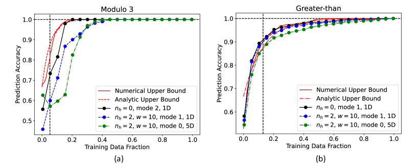
Figure 3: Prediction accuracy vs. training data fraction for learning the relations (a) equivalent modulo 3, and (b) greater-than. We see that applying inductive bias to the decoder MLP architecture (making it simpler while still capable to succeed) improves the performance (reduces the “induction gap” gap relative to the theoretical upper bound). In the legend, $n_{h}$ is the number of hidden layers, $w$ is the width of the hidden layers, mode indicates how the two embeddings are combined, and the dimension is that of the embedding space. Vertical lines show the approximate transition scale $b/n^{2}$.

In Figure 3, we see that the neural generalization curves roughly track our theoretical prediction, with a slightly delayed rise, presumably for the two aforementioned reasons. Also, generalization may occur at a much later training step, due to delayed generalization/grokking.

We term the architecture-dependent part of this delay the inductive gap. Figure 3 illustrates that the inductive gap decreases when it is simplified by including more inductive bias in the model. We will now aim to provide intuition for this finding.

We have defined three modes for combining encoder outputs into decoder input:

1. The default mode, where the input to the decoder is the concatenation of two embeddings $[\mathbf{E}_{x_{1}},\mathbf{E}_{x_{2}}]$,

2. The decoder’s input is $(\mathbf{E}_{x_{1}}-\mathbf{E}_{x_{2}})$, and

3. The decoder’s input is $|\mathbf{E}_{x_{1}}-\mathbf{E}_{x_{2}}|^{2}$, element-wise squared.

For learning equivalence modulo 3, the ideal embedding would be to cluster numbers into three distinct positions on a 1-dimensional line corresponding to the 3 equivalence classes. Hence, one expects the neural network to learn that $P[R(x_{1},x_{2})=1]=1$ iff $\mathbf{E}_{x_{1}}=\mathbf{E}_{x_{2}}$. This is distinguished by mode 3 followed by a single ReLU$(0.1-x)$ activation, say. This embedding and decoder automatically enforce the symmetry, transitivity, and reflexivity of this relation, enabling it to exploit these properties to generalize. Indeed, Figure 3(a) shows that the inductive gap is the smallest for a network in mode 3 with 0 hidden layers. In contrast, the more complex neural networks in the figure waste some of the training data just to learn this useful inductive bias.

For learning the greater-than relation, the ideal encoding would be to embed numbers on a 1-dimensional line in their correct order. Hence, one expects the neural network to learn $P[R(x_{1},x_{2})=1]=1$ iff $({E}_{x_{1}}-{E}_{x_{2}})>0$. This is best learned in mode 2: the relation holds if the decoder’s input is positive – which can be accomplished with a single ReLU activation. Indeed, Figure 3(b) shows that the inductive gap is the smallest for a network in mode 2 with 0 hidden layers. In summary, we have illustrated that applying correct inductive bias to the neural network’s architecture reduces the inductive gap, thereby improving its generalization performance.

4 Optimal Model Complexity for Generalization

Liu et al. (2022a) postulated that encoder-decoder architectures have a Goldilocks zone of decoder complexity such that generalization fails both when the decoder is too simple and when it is too complex. In this section, we validate this conclusion with our graph learning experiments. Let the decoder have $n_{h}$ layers of uniform width $w$ so that the total number of trainable weight and bias parameters is approximately $w^{2}n_{h}$.

Figure 4 shows testing accuracy vs. decoder depth for our example relations. All cases reveal the existence of a (i.e. sweet spot) where generalization occurs, degrading on both sides. When the decoder is too simple, it lacks the ability to correctly decode learned embeddings, thus failing to provide any useful gradient information for the encoder — the result is confusion, with not even the training accuracy becoming good. When the decoder is too complex, it is able to correctly decode even random and extremely inconvenient encodings, again failing to provide any useful gradient information for the encoder — the result is memorization (overfitting), with high training accuracy but low test accuracy.

We see that the Goldilocks zone for learning greater-than relation is slightly off compared to the other three relations. We relate this to the fact that as in Figure 3(a), learning the greater-than relation can easily reach $\approx 90\%$ accuracy, but struggles to reach $100\%$. Since most of the samples can be easily guessed from a few other samples, the test accuracy does not easily go below $90\%$. A small number of samples that cannot be guessed from any other samples, of the form $i<(i+1)$, does not impact the testing accuracy by a noticeable margin.

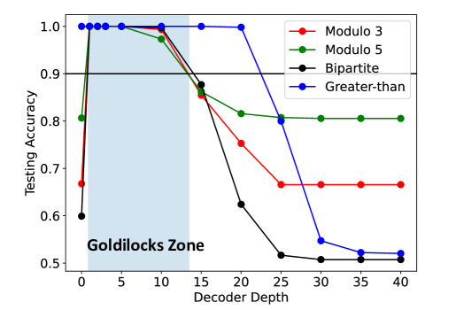
Figure 4: Plot of testing accuracy vs. decoder depth for the four example relations. Decoder width $w=10$, and the training fraction of $0.6$ were used in the experiments.

5 Critical Learning Rates for Generalization

Effective Theory: Interacting Repon Theory As our neural network is trained, the embedding vectors gradually move to hopefully form useful representations. In this section, we study the dynamics of this motion by viewing each representation vector as a “repon” particle, moving in response to interactions with other repons. We show that when the optimal representation involves these particles forming distinct clusters (as for learning e.g.equivalence relations), attraction/repulsion between same-cluster repons corresponds to generalization/overfitting.

Although the global loss landscape of a neural network is typically nonlinear, we consider what happens when two embeddings $\textbf{x}_{1}$ and $\textbf{x}_{2}$ are sufficiently close that the decoder can be locally linearized as $D(\textbf{x})\approx\textbf{A}\textbf{x}+\textbf{b}$. If the two belong in the same cluster, so that the loss function is minimized for $D(\textbf{x}_{1})=D(\textbf{x}_{2})=\textbf{y}$, say, then the training loss for this pair of samples can be approximated as

$$\ell=\frac{1}{2}(|\textbf{A}\textbf{x}_{1}+\textbf{b}-\textbf{y}|^{2}+|\textbf{A}\textbf{x}_{2}+\mathbf{b}-\mathbf{y}|^{2}).$$ (5)

Both the decoder $(\textbf{A},\textbf{b})$ and the encoder (the repon positions $\textbf{x}_{1}$, $\textbf{x}_{2}$) are updated via a gradient flow, with learning rates $\eta_{A}$ and $\eta_{x}$, respectively:

$$\frac{d\mathbf{A}}{dt}=-\eta_{A}\frac{\partial\ell}{\partial\mathbf{A}},\frac{d\mathbf{b}}{dt}=-\eta_{A}\frac{\partial\ell}{\partial\mathbf{b}},\frac{d\mathbf{x}_{i}}{dt}=-\eta_{x}\frac{\partial\ell}{\partial\mathbf{x}_{i}}\ (i=1,2).$$ (6)

Substituting $\ell$ into the above equations simplifying as detailed in Appendix C, we obtain

$$\frac{d\textbf{A}}{dt}=-2\eta_{A}\textbf{A}\textbf{r}\textbf{r}^{T},\;\frac{d\textbf{r}}{dt}=-\eta_{x}\textbf{A}^{T}\textbf{A}\textbf{r},$$ (7)

where $\mathbf{r}\equiv(\mathbf{x}_{1}-\mathbf{x}_{2})/2$ is half the repon separation.

This repon pair therefore interacts via a quadratic potential energy $U(\mathbf{r})=\frac{1}{2}\mathbf{r}^{T}\textbf{A}^{T}\textbf{A}\mathbf{r}$, leading to a linear attractive force $F(\textbf{r})\propto-\textbf{A}^{T}\textbf{A}\textbf{r}$ which is accurate whenever two repons are sufficiently close together. In one embedding dimension, this is like Hookes’ law for an elastic spring pulling the repons together, except that the spring is weakening over time. Eq. (7) has simple asymptotics: (i) If $\mathbf{A}$ is constant or $\eta_{A}=0$, two repons will eventually collide, i.e., $r\to 0$. (ii) In the opposite limit, if $\mathbf{r}$ is constant or $\eta_{x}=0$, A will converge to $\mathbf{0}$ while $r>0$. In the general case where $\eta_{x},\eta_{A}>0$, Eq. (7) is a competition between which of A and r decays faster, whose outcome depends on $\eta_{A}$ and $\eta_{x}$,as well as the initial values of $\mathbf{A}_{0}$ and $\mathbf{r}_{0}$. Without loss of generality, we can rescale the embedding space so that $|\textbf{r}_{0}|=1$.

General case: It is easy to check Eq. (7) has a solution of the following form:

$$\mathbf{A}(t)=a(t)\mathbf{A}_{0}+b(t)\mathbf{A}_{0}\mathbf{r}_{0}\mathbf{r}_{0}^{T},\quad\mathbf{r}(t)=c(t)\mathbf{r}_{0}.$$ (8)

Substituting this into Eq. (7) and defining $a_{2}(t)\equiv a(t)+b(t)$ gives the differential equations

$$\frac{da_{2}}{dt}=-2\eta_{A}c^{2}a_{2},\;\frac{dc}{dt}=-\eta_{x}a_{2}^{2}c,$$ (9)

whose fixed point $(a_{2}^{*},c^{*})$ defined by $da_{2}/dt=0,dc/dt=0$ requires $a_{2}^{*}=0$ or $c^{*}=0$. A repon collision happens if $c^{*}=0$. Interestingly, there is a conserved quantity

$$C\equiv\frac{1}{2\eta_{A}}a_{2}^{2}-\frac{1}{\eta_{x}}c^{2},$$ (10)

because $dC/dt=0$. This defines a hyperbola and the value $C$ is determined by initialization. If $C>0$, $c^{*}\to 0$ and $a_{2}^{*}\to\pm\sqrt{2\eta_{A}C}$, resulting in repon collision (generalization). If $C<0$, $c^{*}\to\pm\sqrt{-\eta_{x}C}$ and $a_{2}^{*}\to 0$, leading to no collision (memorization). When the initial conditions $a_{2}^{(0)}$ and $c^{(0)}$ are drawn from a normal distribution with width $\sigma_{a}$ and $\sigma_{c}$ respectively, the probability of representation learning (i.e., $c^{*}\to 0$) is

$$p_{r} =\underset{\frac{c}{a}<\sqrt{\frac{\eta_{x}}{2\eta_{A}}}}{\iint}\frac{1}{2\pi\sigma_{a}\sigma_{x}}{\rm exp}\left(-\frac{1}{2}\left[\left(\frac{a}{\sigma_{a}}\right)^{2}+\left(\frac{c}{\sigma_{c}}\right)^{2}\right]\right)dadc$$ (11)

$$=\frac{2}{\pi}{\rm arctan}\left(\frac{\sigma_{a}}{\sigma_{c}}\sqrt{\frac{\eta_{x}}{2\eta_{A}}}\right),$$

which provides a practical prescription for enhancing representation learning. Below, we provide empirical evidence that supports this theory.

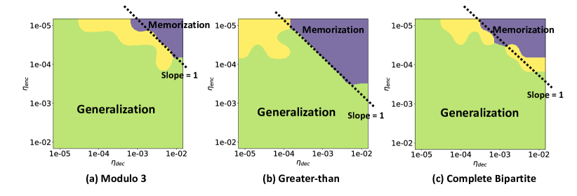
Figure 5: Phase diagram as a function of the encoder learning rate $\eta_{\textrm{enc}}$ and decoder learning rate $\eta_{\textrm{dec}}$ for (a) modulo 3, (b) greater-than, and (c) complete bipartite relations. All figures indicate a slope-1 boundary between the generalization and memorization phases, as predicted by the interacting repon theory. Green, yellow, and purple regions indicate the generalization, delayed generalization (grokking), and memorization phase respectively.

Neural Network Experiments: Figure 5 shows the generalization/memorization phase diagram as a function of the encoder learning rate $\eta_{\textrm{enc}}$ and the decoder learning rate $\eta_{\textrm{dec}}$ for different relations. Phase classification criteria are described in Appendix B. Generalization can be interpreted as the probability of representation learning in Eq.(11) exceeding a certain threshold. Hence, in a phase diagram as a function of encoder and decoder learning rates with logarithmic axes, one would expect the generalization-memorization boundary to have slope $-1$, which is indeed observed in Figure 5. Moreover, the phase boundary appears approximately at the same intercept, which also matches the prediction of Eq. 11 that the probability of representation learning should be task-independent, and only depends on the weight initialization. As a rule of thumb, we see that generalization requires that the learning rate product $\eta_{\textrm{enc}}\eta_{\textrm{dec}}\mathrel{\hbox to0.0pt{\lower 3.0pt\hbox{$\mathchar 536\relax$}\hss}\raise 2.0pt\hbox{$\mathchar 316\relax$}}10^{-7}$. We provide additional phase diagrams in Appendix D that further validate the interacting repon theory.

6 Related Work

Physics of Machine Learning: Physics-based methodologies have been widely used to develop theories for deep learning. These include employing effective theories (Roberts et al., 2022; Halverson et al., 2021), conservation laws (Kunin et al., 2020), and general paradigms in statistical physics such as phase diagrams and free-energy principle (Gao & Chaudhari, 2020; Liu et al., 2022a; b). Our work provides a physics-inspired framework for understanding generalization, where the dynamic properties of generalization are described by studying the physics of interacting particles whose positions are given by their positions in the embedding space.

Model Generalizability in Machine Learning: There is a rich literature on studying out-of-distribution generalization (Liu et al., 2021; Ye et al., 2021). However, most of these studies focus on empirically extracting invariant features over multiple domains and lack an analysis of why and when generalization occurs. Our study attempts to fill this gap by pursuing a unifying effective theory. Our study also complements the previous studies on generalization in learning modular addition (Liu et al., 2022a; b) by presenting theories and empirical results for general mathematical relations.

Learning Mathematical Relations: Machine learning has been utilized to understand various mathematical entities, such as geometry (He, 2023) and knot theory (Gukov et al., 2021). Our work provides physics-based effective theories for understanding how neural networks learn mathematical relations.

7 Conclusion

We have presented an effective theory framework for understanding the statics and dynamics of model generalization in practice. In particular, we have studied the minimal data size needed, optimal model complexity, and critical decoder learning rates for generalization. While some static properties could be quite well described by our effective theory, incorporating more information about the input data’s structures into the theory may contribute to further bridging the theory-experiment gap. There is ultimately a trade-off between the complexity of the theory and its accuracy. In this regard, we believe our information-theory-based approximation is helpful for understanding static properties of generalization. The theory of dynamic properties for generalization was largely well-supported by the relevant empirical phase diagrams.

Our study suggests the following unifying framework for understanding generalization: static properties of generalization can be derived from information-theoretic properties of the input data, while the dynamic properties of generalization can be understood by studying the system of interacting particles, repons. Our work also highlights the power of physics-inspired effective theories for bridging the gap between theoretical predictions and practice in machine learning.

Data and Code Availability

We will provide data and codes upon request.

Acknowledgments

We thank the Center for Brains, Minds, and Machines (CBMM) for hospitality. This work was supported by The Casey and Family Foundation, the Foundational Questions Institute, the Rothberg Family Fund for Cognitive Science and IAIFI through NSF grant PHY-2019786.

Appendix A List of Default Hyperparameter Values

The hyperparameter values below were used for the experiments unless specified otherwise.

Table 3: List of default hyperparameter values.

Parameter	Default Value
Embedding Space Dimension	2
Weight Decay	0
Learning Rate	0.001
Training Data Fraction	0.75
Decoder Depth	3
Decoder Width	50
Activation Function	Tanh

Appendix B Definition of Phases

We have followed the phase classification criteria of Liu et al. (2022a).

Table 4: Phase classification criteria.

	Criteria
Phase	train acc $>0.9$	test acc $>0.9$	(steps to test acc $>0.9$)
	within $10^{5}$ steps	within $10^{5}$ steps	$-$ (steps to train acc $>0.9$) $<$ $10^{3}$
Generalization	Yes	Yes	Yes
Grokking	Yes	Yes	No
Memorization	Yes	No	N/A
Confusion	No	No	N/A

Appendix C Derivation of Eq. (7)

The gradient flow is:

$$\frac{d\mathbf{A}}{dt}=-\eta_{A}\frac{\partial\ell}{\partial\mathbf{A}}=-\eta_{A}[\mathbf{A}(\mathbf{x}_{1}\mathbf{x}_{1}^{T}+\mathbf{x}_{2}\mathbf{x}_{2}^{T})+(\mathbf{b}-\mathbf{y})(\mathbf{x}_{1}+\mathbf{x}_{2})^{T}],$$ (12)

$$\frac{d\mathbf{b}}{dt}=-\eta_{A}\frac{\partial\ell}{\partial\mathbf{b}}=-\eta_{A}(\mathbf{A}(\mathbf{x}_{1}+\mathbf{x}_{2})+\mathbf{b}-\mathbf{y})$$

$$\frac{d\mathbf{x}_{i}}{dt}=-\eta_{x}\frac{\partial\ell}{\partial\mathbf{r}}=-\eta_{x}\mathbf{A}^{T}(\mathbf{A}\mathbf{x}_{i}+\mathbf{b}-\mathbf{y}),\ (i=1,2).$$

Without loss of generality, we can choose the coordinate system such that $\mathbf{x}_{1}+\mathbf{x}_{2}=\mathbf{0}$. For the $d\mathbf{b}/dt$ equation: setting the initial condition $\mathbf{b}(0)=\mathbf{0}$ gives $\mathbf{b}(t)=(1-e^{-2\eta_{A}t})\mathbf{y}$. Inserting this into the first and third equations gives

$$\frac{d\mathbf{A}}{dt}=-2\eta_{A}\mathbf{A}\mathbf{r}\mathbf{r}^{T}$$ (13)

$$\frac{d\mathbf{x}_{i}}{dt}=-\eta_{x}\mathbf{A}^{T}\mathbf{A}\mathbf{x}_{i}+\eta_{x}e^{-2\eta_{A}t}\mathbf{A}^{T}\mathbf{y}$$

Now define the relative position $\mathbf{r}\equiv(\mathbf{x}_{1}-\mathbf{x}_{2})/2$ and subtracting $d\mathbf{x}_{1}/dt$ by $d\mathbf{x}_{2}/dt$ we get:

$$\frac{d\mathbf{A}}{dt}=-2\eta_{A}\mathbf{A}\mathbf{r}\mathbf{r}^{T},$$ (14)

$$\frac{d\mathbf{r}}{dt}=-\eta_{x}\mathbf{A}^{T}\mathbf{A}\mathbf{r}.$$

Appendix D Additional Phase Diagrams

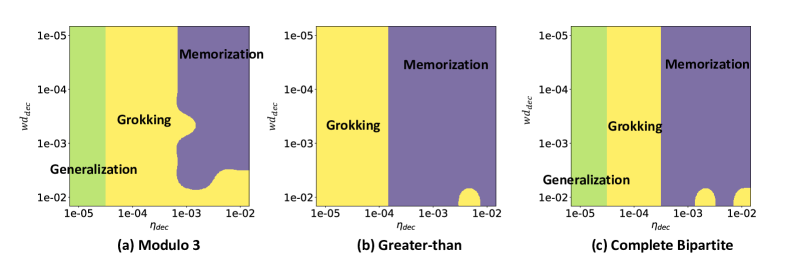
Figure 6: Phase diagram as a function of the decoder’s weight decay $wd_{\textrm{dec}}$ and the decoder’s learning rate $\eta_{\textrm{dec}}$ for (a) modulo 3, (b) greater-than, and (c) complete bipartite relations. All figures indicate that the memorization-generalization boundary is independent of the weight decay, which is consistent with the result of interacting repon theory in Eq. (11). Note that grokking is also a form of generalization, but the delayed generalization. Encoder’s learning rate was fixed to $\eta_{\textrm{enc}}=10^{-5}$ in the experiment.

References

- Bejani & Ghatee (2021) Mohammad Mahdi Bejani and Mehdi Ghatee. A systematic review on overfitting control in shallow and deep neural networks. Artificial Intelligence Review, pp. 1–48, 2021.
- Gao & Chaudhari (2020) Yansong Gao and Pratik Chaudhari. A free-energy principle for representation learning. In International Conference on Machine Learning, pp. 3367–3376. PMLR, 2020.
- Gukov et al. (2021) Sergei Gukov, James Halverson, Fabian Ruehle, and Piotr Sułkowski. Learning to unknot. Machine Learning: Science and Technology, 2(2):025035, 2021.
- Halverson et al. (2021) James Halverson, Anindita Maiti, and Keegan Stoner. Neural networks and quantum field theory. Machine Learning: Science and Technology, 2(3):035002, 2021.
- He (2023) Yang-Hui He. Machine-learning mathematical structures. International Journal of Data Science in the Mathematical Sciences, 1(01):23–47, 2023.
- Kunin et al. (2020) Daniel Kunin, Javier Sagastuy-Brena, Surya Ganguli, Daniel LK Yamins, and Hidenori Tanaka. Neural mechanics: Symmetry and broken conservation laws in deep learning dynamics. arXiv preprint arXiv:2012.04728, 2020.
- Liu et al. (2021) Jiashuo Liu, Zheyan Shen, Yue He, Xingxuan Zhang, Renzhe Xu, Han Yu, and Peng Cui. Towards out-of-distribution generalization: A survey. arXiv preprint arXiv:2108.13624, 2021.
- Liu et al. (2022a) Ziming Liu, Ouail Kitouni, Niklas S Nolte, Eric Michaud, Max Tegmark, and Mike Williams. Towards understanding grokking: An effective theory of representation learning. Advances in Neural Information Processing Systems, 35:34651–34663, 2022a.
- Liu et al. (2022b) Ziming Liu, Eric J Michaud, and Max Tegmark. Omnigrok: Grokking beyond algorithmic data. arXiv preprint arXiv:2210.01117, 2022b.
- Roberts et al. (2022) Daniel A Roberts, Sho Yaida, and Boris Hanin. The principles of deep learning theory. Cambridge University Press Cambridge, MA, USA, 2022.
- Ye et al. (2021) Haotian Ye, Chuanlong Xie, Tianle Cai, Ruichen Li, Zhenguo Li, and Liwei Wang. Towards a theoretical framework of out-of-distribution generalization. Advances in Neural Information Processing Systems, 34:23519–23531, 2021.