Efficient Stagewise Pretraining via Progressive Subnetworks

Abstract

Recent developments in large language models have sparked interest in efficient pretraining methods. A recent effective paradigm is to perform stagewise training, where the size of the model is gradually increased over the course of training (e.g. gradual stacking (J. Reddi et al., 2023)). While the resource and wall-time savings are appealing, it has limitations, particularly the inability to evaluate the full model during earlier stages, and degradation in model quality due to smaller model capacity in the initial stages. In this work, we propose an alternative framework, progressive subnetwork training, that maintains the full model throughout training, but only trains subnetworks within the model in each step. We focus on a simple instantiation of this framework — Random Path Training (RaPTr) — that only trains a sub-path of layers in each step, progressively increasing the path lengths in stages. RaPTr achieves better pre-training loss for BERT and UL2 language models while requiring 20-33% fewer FLOPs compared to standard training, and is competitive or better than other efficient training methods. Furthermore, RaPTr shows better downstream performance on UL2, improving QA tasks and SuperGLUE by 1-5% compared to standard training and stacking. Finally, we provide theoretical basis for RaPTr to justify (a) the increasing complexity of subnetworks in stages, and (b) the stability in loss across stage transitions due to residual connections and layer norm.

1 Introduction

Large network based language models (e.g. Transformers) have revolutionized the field of NLP. Intriguingly, these language models have demonstrated remarkable emergent abilities that only begin to manifest at large scales (Wei et al., 2022; Schaeffer et al., 2023). However, training such large models is usually very slow and resource intensive (Brown et al., 2020; Touvron et al., 2023; Chowdhery et al., 2022). This has sparked interest in efficient training of large models, necessitating the development of new algorithms and paradigms for efficient pretraining. Traditionally, this was accomplished by designing better optimization algorithms (e.g., Liu et al. 2023a; Chen et al. 2023; Gupta et al. 2018; Shazeer and Stern 2018) that require fewer training steps to reduce the loss. Recently, other paradigms such as stagewise training have garnered interest. These approaches train large models in stages, starting with cheaper training in the early stages, which can find a good initializer for expensive later stages. This powerful framework has shown to drastically reduce the training iterations and FLOPs needed to train large models.

Progressive stacking (Gong et al., 2019) and gradual stacking (J. Reddi et al., 2023) are instantiations of stagewise training. Progressive stacking starts with a small network and doubles the number of layers in each stage by stacking the parameters of the previous stage onto itself, whereas gradual stacking increases the network depth in a slower manner, until the desired depth is reached. While these stacking approaches have shown to be effective in reducing the FLOPs and wall-clock time, the training performance is found to be sensitive to the (stacking) schedules, thus requiring a careful grid search. Furthermore, since the model grows gradually, it is not possible to assess the full model performance during earlier stages (i.e., it is not an anytime algorithm). Additionally, using small model with way fewer parameters for part of the training can hamper model quality (e.g. long term memory (Geva et al., 2021)), especially for single epoch training where each data sample is seen once during training. It is indeed observed in our experiments (§4.2) that the pretraining loss and downstream performance may be worse than baseline training at equal FLOPs.

In this paper, we propose a novel stagewise training approach called progressive subnetwork training that addresses some of the above issues. Unlike stacking, where different stages train models of different sizes, we maintain a common base model of interest and train subnetworks of varying complexities within this model. Motivated by the phenomenon that gradient-based training learns functions of increasing complexity over time (Kalimeris et al., 2019; Abbe et al., 2022), we progressively increase the complexity of subnetworks in each stage to explicitly impose this simple-to-complex behavior. As a concrete instantiation of this framework, we choose subnetworks to be paths comprised of a subset of layers, and in each stage we perform forward and backward passes over a random subset of layers. This can be achieved using a simple recipe: (a) drop out layers randomly with certain probability during forward and backward passes, and (b) progressively decrease the dropout probability to zero over time according to a fixed schedule. We name this approach Random Path Training (RaPTr). Our approach reduces the total number of FLOPs in the initial stages, but unlike stacking, every parameter of the full model contributes to the training loss at all stages, and it allows us to track the full model throughout training. This simple strategy turns out to be very effective for training efficiency and improving model quality.

It is worth noting that the idea of dropping some layers during training has been explored in the literature but mainly as a regularization strategy or for improving inference efficiency (Fan et al., 2019; Zhang et al., 2019; Liu et al., 2023c). The closest work for training efficiency is progressive layer dropping (Zhang and He, 2020), where FLOPs are saved by increasingly dropping more layers as training proceeds – exactly the opposite of progressive subnetworks. In fact, a subsequent work (Kaddour et al., 2023) shows that such a schedule can hurt pre-training performance after careful evaluations. In this paper, we confirm this observation by showing theory and experiments that there is a fundamental difference between this strategy and RaPTr: RaPTr can effectively learn complex correlations in the data in stages, but dropping more layers later during training can be detrimental to learning those complex correlations. Our main contributions are as follows:

• We introduce a novel stagewise training called progerssive subnetworks in §2 that enables tracking the performance of the final model in all stages. Specifically we explore Random Path training (RaPTr) that trains a path comprised of a random subset of layers, with the average length of path progressively increasing in stages.

  

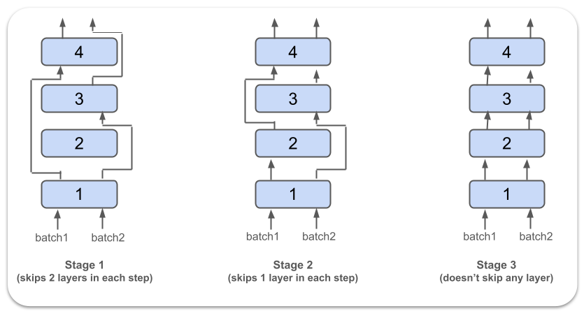
  Figure 1: Pictorial description of stagewise RaPTr where the number of layers being skipped progressively decreases over stages.

• Through analysis on polynomial data in §3, we study the role of progressive training and show (with experiments and theory), that progressive RaPTr can effectively learn higher degree components in a stage-wise manner, whereas progressive layer dropping can be detrimental for higher order terms. This provides a justification for progressively increasing complexity in stages.

• We conduct extensive experiments to compare gradual stacking, progressive layer dropping and RaPTr on BERT (Devlin et al., 2018) and UL2 language models. On BERT-Base, RaPTr demonstrates notable improvements in the pretraining loss when compared to gradual stacking at similar FLOPs, while being better than baseline training with $33\%$ fewer FLOPs. The benefits of RaPTr are especially significant in the short horizon setting (few epoch training). For UL2-$1.6B$ language model (Tay et al., 2022), RaPTr can match the pretraining perplexity of baseline training with 20% fewer FLOPs. Interestingly, at the same perplexity we observe significant improvements in downstream evaluations, e.g. we see 3-5% absolute increase in $1$-shot exact match scores on TydiQA (Clark et al., 2020) and SQuADv2 (Rajpurkar et al., 2018) compared to baseline and gradual stacking.

• We provide a theoretical study for conditions under which RaPTr yields smooth transition in loss across stage transitions (§5), by characterizing a stability condition with respect to dropping of layers. Illustrative examples with linear networks are presented to show how layernorm and residual connections can help with this stability.

2 Progressive subnetwork training

Notation. $[n]$ denotes the set $\{1,2,\dots,n\}$. $a_{1:k}$ is used to denote a sequence of $k$ scalars $a_{1},\dots,a_{k}\in\mathbb{R}$. ${\bm{x}}$ denotes a vector in $\mathbb{R}^{d}$ . ${\bm{x}}_{1:k}$ denotes a sequence of $k$ vectors ${\bm{x}}_{1},\dots,{\bm{x}}_{k}\in\mathbb{R}^{d}$. We use ${\bm{X}}\in\mathbb{R}^{n\times d}$ to denote a matrix containing a sequence ${\bm{x}}_{1:n}$ as rows. We consider the setting where the goal is to learn an $L$-layer sequence-to-sequence neural network. (e.g., standard Transformer network).

Definition 2.1 ($L$-layer sequence-to-sequence model).

Let $f_{1},\cdots,f_{L}:\mathbb{R}^{N\times d}\to\mathbb{R}^{N\times d}$ denote a set of $L$ sequence-to-sequence functions. Then, $F:\mathbb{R}^{N\times d}\times\mathbb{R}^{L}\to\mathbb{R}^{N\times d}$ takes an input sequence ${\bm{X}}\in\mathbb{R}^{N\times d}$, scalars $\alpha_{1:L}$, and outputs a sequence ${\bm{Y}}$ defined recursively with intermediate outputs ${\bm{Y}}^{(1)},\cdots,{\bm{Y}}^{(L-1)},{\bm{Y}}^{(L)}$ as

$${\bm{Y}}^{(\ell)}={\bm{Y}}^{(\ell-1)} +\alpha_{\ell}f_{\ell}({\bm{Y}}^{(\ell-1)})\text{ for all }1\leq\ell\leq L,$$

$$F({\bm{X}};\alpha) ={\bm{Y}}^{(L)},$$ (1)

where ${\bm{Y}}^{(0)}$ denotes ${\bm{X}}$, ${\bm{Y}}^{(\ell)}$ is the output of $\ell$-th layer.

Standard model training uses scalars $\alpha_{i}=1$ for $i\in[L]$. For simplicity, we use $F({\bm{X}})$ to denote the output and ${\bm{Y}}^{(1)},{\bm{Y}}^{(2)},\cdots,{\bm{Y}}^{(L)}$ as the intermediate layer outputs of $F$ under standard model training, unless specified otherwise.

Progressive subnetwork training is a stagewise training framework that consists of two crucial components:

1. Subnetwork selection: At each iteration, we select a (possibly random) subnetwork of the $L$-layer neural network. The forward and backward passes are computed based on this subnetwork.

2. Progressive subnetwork sizes: The size of the subnetworks being trained is progressively increased in a stagewise manner, starting from small subnetworks and ending with the full network in the final stage.

Note that this framework is quite general since subnetworks could be selected along any dimension of the model, e.g., attention heads, subset of hidden neurons in MLP layers. In this work, we primarily focus on depth.

Algorithm 1 $k$-stage RaPTr

0:  Blocks $f_{\theta_{1}},\cdots,f_{\theta_{L}}$, Schedule $T_{1:k}\times(p_{1:k},\mathcal{I}_{1:k})$, total steps $T$, data distribution $D$.

  Initialize $\theta_{1},\cdots,\theta_{L}$, $T_{k+1}=T$.

  for $s=1\to k$ do

     for $t=T_{s}\to T_{s+1}$ do

        Sample batch $({\bm{X}},{\bm{Y}})\sim D$.

        Sample $\zeta_{i}\sim B(p)$ for $i\not\in\mathcal{I}_{s}$, set $\zeta_{i}=1$ for $i\in\mathcal{I}_{s}$.

        Set ${\bm{Y}}^{(0)}\leftarrow{\bm{X}}$

        for $j=1\to L$ do

           ${\bm{Y}}^{(j)}\leftarrow{\bm{Y}}^{(j-1)}$

           if   $\zeta_{j}$: ${\bm{Y}}^{(j)}\leftarrow{\bm{Y}}^{(j)}+\zeta_{j}f_{\theta_{j}}({\bm{Y}}^{(j-1)})$

        end for

        Compute loss with ${\bm{Y}}^{(L)}$ and take a optimizer step.

     end for

  end for

2.1 Random Path Training: RaPTr

One simple strategy to select a subnetwork is by choosing a path formed by a subset of layers within the model. More concretely, given a network $F$ to be trained, we pick a random subset of layers for the forward pass and bypass the rest of the layers using the residual connections. We call this approach Random Path Training (RaPTr).

More concretely, let $p$ denote the probability of randomly selecting a layer and $\mathcal{I}$ denote a subset of layers that are always included, i.e. they are never bypassed. We define a random subnewtork before describing RaPTr in more detail.

Definition 2.2 ($(p,\mathcal{I})$-subnetwork).

Let $\zeta_{1:L}$ be Bernoulli samples, with $\zeta_{i}=1$ for all $i\in\mathcal{I}$, while $\zeta_{i}\sim B(p)$ for all $i\not\in\mathcal{I}$. The set of all layers for which $\zeta_{i}=1$ represents a random subnetwork while layers with $\zeta_{i}=0$ are bypassed. The output of the selected subnetwork on a sequence input ${\bm{X}}$ is equivalent to the output of the model given by $F({\bm{X}},\zeta_{1:L})$ as defined in Equation 1.

Stagewise progressive RaPTr. The pseudo-code for RaPTr is provided in Algorithm 1. At a high level, the total training is split into $k$ stages. Each stage $s$ uses $(p_{s},\mathcal{I}_{s})$-subnetwork between steps $T_{s}$ and $T_{s+1}$. We denote this schedule by $T_{1:k}\times(p_{1:k},\mathcal{I}_{1:k})$. Importantly, we progressively increase the random subnetwork selection pattern across stages i.e., the expected length of the selected random subnetworks is increased progressively towards full model training. This can be achieved by either increasing the probability of including each layer in random subnetwork or fixing more layers in $\mathcal{I}_{\cdot}$ or both. More formally, we use schedules $T_{1:k}\times(p_{1:k},\mathcal{I}_{1:k})$ that satisfies: (a) $p_{s}\leq p_{\tilde{s}}$, and (b) $\mathcal{I}_{s}\subseteq\mathcal{I}_{\tilde{s}}$ for all $1\leq s\leq\tilde{s}\leq k$.

Training efficiency. Training step in RaPTr involves computing forward and backward passes only on random subnetwork. In expectation, training a $(p,\mathcal{I})$ random subnetwork will require $\frac{\left|\mathcal{I}\right|+(L-\left|\mathcal{I}\right|)p}{L}$ FLOPs relative to standard training that uses all $L$ layers. By using $p\ll 1$ for majority of training, RaPTr can improve training efficiency.

Connection to progressive layer dropping (PLD). We note that RaPTr bears resemblance with progressive layer dropping (Zhang and He, 2020), where idea is to drop more layers as training proceeds for FLOPs efficiency (see §A.1 for details). In fact, this is in sharp contrast to progressive RaPTr, where we drop fewer layers as training proceeds. While this difference may seem superficial at first, it has deep implications from both conceptual and performance standpoints. In §3, we argue through theoretical and empirical analysis on polynomial data, that this can have very significant impact on learning complex correlations in data. In the BERT and UL2 experiments in §4, we similarly observe that progressive layer dropping performs significantly worse than RaPTr.

3 Illustration: RaPTr in polynomial setting

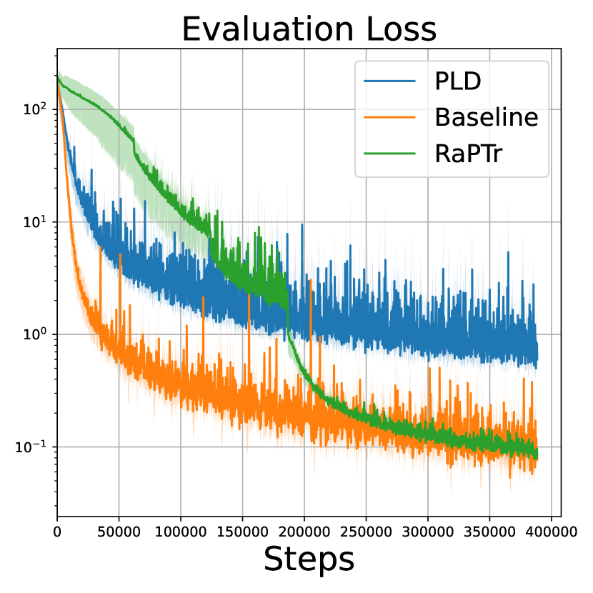
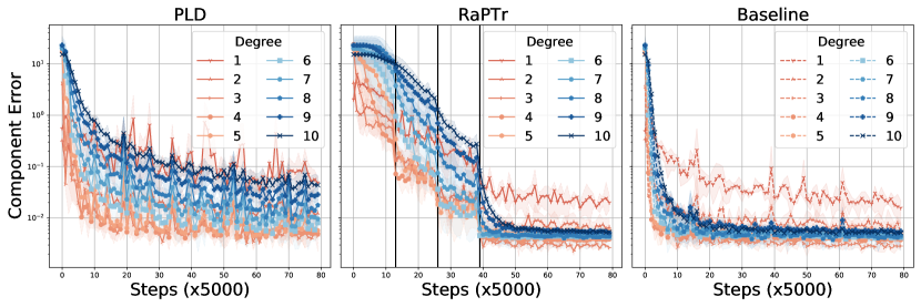
Figure 2: Evaluation loss (left) and component error (3 on the right) on basis polynomials of different degrees for a $20$ layer residual network trained with different methods. Labels are generated from a composition of polynomials of degrees $1$ to $10$ (Eq.2). The schedules for RaPTr and PLD are selected to have 20% fewer FLOPs compared to baseline (phase transitions for RaPTr have been marked with dark vertical lines). (more details in §A.2). Observations: (a) RaPTr reaches same evaluation loss of baseline, while PLD performs much worse. (b) RaPTr learns lower order terms faster and picks up higher order terms in the later stages. PLD is worse at capturing higher degree terms owing to its reduced expressivity towards the end.

In this section, we discuss the importance of the progressive nature of training in RaPTr and sharply contrast it with PLD. While both these strategies improve training efficiency, we ask an important question: what schedule of subnetwork size works better? We demonstrate the importance of progressively increasing the complexity of subnetworks in RaPTr (as opposed to progressively decreasing it PLD) through a simple, yet instructive, setting: learning neural networks on polynomial data. For simplicity, we restrict the discussion to sequences of length $N=1$.

Polynomial learning setting. Suppose ${\bm{x}}$ are sampled from a uniform distribution over $\{\pm 1\}^{d}$. The ground-truth label is a polynomial $f^{\star}$ of degree $k$ defined as

$$F^{\star}({\bm{x}})=\sum_{l=1}^{k}\sum_{j=1}^{m}c_{l,j}\prod_{i\in S_{l,j}}x_{i},$$ (2)

where $c_{l,j}\sim\mathcal{N}(0,1)$ and $S_{l,j}$ are random subsets of $[d]$ of cardinality $\ell$. Such polynomials have been studied in great detail (Abbe et al., 2022, 2023) where the higher degree terms capture more complex correlations and are harder to learn. We consider training of $20$-layer residual network (He et al., 2016) $F$ on such data using square loss: $\mathbb{E}(F({\bm{x}})-F^{\star}({\bm{x}}))^{2}$. Here each residual block consists of a single $4d$-hidden dimension MLP layer with ReLU activation.

Empirical Observations. We are interested in measuring how well each method captures the higher degree terms. To this end, we estimate the component of a learned function $F$ onto each basis polynomials. This can be done simply using $\hat{c}_{l,j}=\mathbb{E}_{{\bm{x}}\sim\{\pm 1\}^{d}}\left[F({\bm{x}})\prod_{i\in S_{l,j}}x_{i}\right],$ since basis polynomials are orthogonal under the uniform distribution of the boolean data (O’Donnell, 2014). For each degree $l\leq k$, we define the error as $\tfrac{\sum_{j=1}^{m}(c_{l,j}-\hat{c}_{l,j})^{2}}{\sum_{j=1}^{m}c_{l,j}^{2}}$. In Figure 2, we observe the following:

• RaPTr is competitive to baseline in terms of evaluation loss; in fact, RaPTr learns every component effectively. Furthermore, RaPTr quickly learns lower order terms and then picks up higher order terms during later stages.

• PLD, that drops more layers as training proceeds, fails to effectively learn higher order complex correlations and, ultimately, hurts performance.

The learning pattern of RaPTr is reminiscent of the implicit bias of standard SGD training to learn functions of increasing complexity (Kalimeris et al., 2019; Xu et al., 2019; Rahaman et al., 2019; Cao et al., 2019; Abbe et al., 2022). RaPTr naturally imposes this simple-to-complex behavior through size of subnetworks and also provides training efficiency in the process.

Theoretical Analysis. To further illustrate our point, we characterize the behavior of RaPTr for a simple 2-layer residual network, where each block consists of single neuron with a non-linear sine activation. We consider simple label function $F^{\star}({\bm{x}})=\frac{\sqrt{3}}{2}+\frac{\sqrt{3}}{2}x_{1}-x_{1}x_{2}$ for this analysis.

Lemma 3.1 (Informal, cf Theorem E.1).

For a small enough learning rate, 2-phase RaPTr first learns lower degree component and then the higher degree component.

In constrast, one layer is not expressive enough to represent the true label function (E.2). Thus, progressively dropping more layers (e.g., PLD) will reduce its expressivity.

4 Experiments

In this section, we present comprehensive experiments that compare RaPTr with standard baseline training, gradual stacking and progressive layer dropping (PLD) for BERT and UL2. We primarily choose stacking for comparisons given the recent findings in Kaddour et al. (2023) that show stacking to be the best (and only) efficient training method that can beat baseline over different training horizons.

Few additions to RaPTr: We make few additions to RaPTr described in Section 2.1. We keep $\mathcal{I}$ equal to the first and last layer ($\mathcal{I}=\{1,L\}$) across all stages. Furthermore, we observed that appropriately scaling layer outputs for the selected layers during initial stages helps track the validation loss better (Fig. 6 in appendix); we defer the details to the appendix (Appendix F) since the final effect of this scaling was minimal. Finally, following gradual stacking (J. Reddi et al., 2023), we train with a constant learning rate in all phases except in the final phase of full model training where we decay the learning rate. This change in learning rate primarily helped in BERT pre-training.

Notations for RaPTr and stacking schedules. We succinctly denote the stage schedules by a set of subnetwork lengths separated by hyphens. For gradual stacking, 6-12-18-24 refers to $4$ stages with a $6$, $12$, $18$ and $24$ layer model training respectively. For RaPTr training with a $24$-layer model, 6-12-18-24 refers to $4$ stages, with probability $p$ set in each stage such that the average length of subnetworks is $6,12,18,$ and $24$ respectively. The length of each stage is chosen based on the reduction in FLOPs to achieve during training (see §B). Unless specified otherwise, we maintain an equal number of training steps for each stage.

4.1 Experiments with BERT

Experiment setup. We pretrain BERT models (Devlin et al., 2018) on Wikipedia + Books dataset with AdamW optimizer (Loshchilov and Hutter, 2019). For all the experiments with BERT-Base and BERT-Large, the total number of training steps is set to 675K and 1M steps, respectively. We report the evaluation loss and fine-tuning performance of the trained models on $3$ GLUE tasks (Wang et al., 2018). Please see §A for more experimental details.

Table 1: Loss and fine-tuning results for BERT-Base after $675$K steps and using equal peak learning rate ($10^{-4}$). Key observations: (a) RaPTr achieves similar loss as baseline at $75\%$ reduced FLOPs. (b) RaPTr achieves $0.02$ better evaluation loss than gradual stacking for same schedules. (c) RaPTr has a slight edge on downstream fine-tuning task.

	Rel.	Eval
Method	FLOPs	Loss	MNLI	QNLI	SST-2	Avg.
Baseline	1.33	1.76	81.5	90.5	91.4	87.8
PLD	1.	1.8	81.7	89.0	90.8	87.2
Stacking
6-8-10-12	1	1.78	-	-	-	-
6-9-12	1	1.77	80.9	89.8	91.1	87.3
RaPTr
6-8-10-12	1	1.75	82.1	89.8	92.4	88.1
6-9-12	1	1.75	82.3	89.2	91.0	87.5

Results at equal training steps. We observe that RaPTr achieves similar or better evaluation loss to baseline training, despite baseline training using $33\%$ more FLOPs than RaPTr for BERT-Base. Compared to gradual stacking at similar FLOPs, RaPTr again has better validation loss. Additionally, all three methods exhibit similar performance in downstream fine-tuning tasks (see Table 1). However, PLD performs significantly worse compared to others.

Results at equal FLOPs. Inspired by Kaddour et al. (2023), we further compare RaPTr and gradual stacking to baseline training by adjusting the number of training steps of baseline training to match its FLOPs to RaPTr. In Table 2, we compare these methods at three different FLOPs budgets. For BERT-Base, we observe that at shorter FLOP experiments, RaPTr achieves much better validation loss compared to baseline training and gradual stacking. This difference gets smaller as we move to larger horizon settings. Similar findings for BERT-Large.

Ablations with RaPTr parameters: We observe robustness of the final trained model to different RaPTr schedules (Tab. 6 in appendix). Furthermore, we observe that fixing the first and last layers at all steps during training helps RaPTr (Tab. 7 in appendix).

Table 2: Equal FLOPs comparisons for BERT-Base and BERT-Large with extensive peak LR tuning. For BERT-Base we use the best performing schedules 6-8-10-12 for RaPTr and 6-9-12 for stacking from Table 1. For BERT-Large, we use 6-12-18-24 for both RaPTr and stacking. FLOPs denotes the number of steps involved in baseline training. Key observations: for BERT-Base (a) RaPTr achieves better loss compared to baseline at all FLOP measures, with larger differences for fewer FLOPs. (b) RaPTr has $0.02$ better loss than gradual stacking at all FLOP levels. (c) For BERT-Large, stacking and RaPTr are competitive to each other at all FLOP counts. Both methods have better loss than baseline at lower FLOP measures.

Model	FLOPs	Baseline	Stacking	RaPTr
BERT-Base	$75k$	2.09	2.02	2.01
	$170k$	1.90	1.88	1.86
	$510k$	1.74	1.75	1.73
BERT-Large	$62.5k$	1.84	1.78	1.80
	$140k$	1.63	1.60	1.61
	$625k$	1.40	1.41	1.41

Table 3: Validation loss and 1-shot downstream evals on UL2-1.6B. Key observations: (a) RaPTr with 30k initial training improves performance by atleast $2-4\%$ on Trivia QA and SquADv2. RaPTr is atleast $5\%$ better than gradual stacking on various downstream tasks, (b) Compared to baseline, RaPTr is $1-2\%$ better on all downstream tasks on average. Decaying the learning rate from the start still retains the benefit of RaPTr. (c) Stagewise training achieves ($1-2\%$) lower variance on Tydi QA and SquADv2, implying implicit benefits of stagewise training.

Method	Rel. FLOPs	Eval Loss	Trivia QA	Tydi QA	SQuADv2	SuperGLUE	Avg. Downstream
Baseline	1.2	2.06 (0.01)	25.0 (0.2)	34.4 (3.1)	42.1 (2.9)	60.0 (0.4)	40.4
PLD	1	2.09 (0.00)	21.3 (0.3)	32.4 (2.1)	40.2 (0.9)	59.9 (0.2)	38.5
12-16-20-24 Stacking	1	2.08 (0.00)	20.1 (1.3)	28.6 (2.4)	36.0 (1.9)	60.4 (0.9)	36.3
12-16-20-24 RaPTr	1	2.08 (—-)	22.2 (—)	38.2 (—)	40.6 (—)	60.1 (—)	40.3
(+30k initial full-model train)	1	2.06 (0.00)	25.8 (0.2)	36.7 (1.0)	44.1 (0.5)	60.9 (0.2)	41.9
(+Unmodified LR)	1	2.07 (0.00)	23.7 (0.4)	35.2 (0.7)	43.8 (0.2)	60.5 (0.9)	40.8

Table 4: We extensively compare all trained models from Table 3 on multiple downstream tasks and few-shot in-context settings. We follow prompt design from Chowdhery et al. (2022) in each setting. For tasks marked with ^† and ^⋆, we report Exact match and F1 scores respectively. For the rest, we use accuracy. The tasks have been sub-divided into 4 major groups, memorization QA, QA with context, completion, and SuperGLUE. On average, RaPTr is 1-2% better than baseline and stacking.

	1-shot				5-shot
	Baseline	RaPTr	Stacking	RaPTr	Baseline	RaPTr	Stacking	RaPTr
				(+30k initial full-model train)				(+30k initial full-model train)
Trivia QA†	25.0 (0.2)	22.2 (—)	20.1 (1.3)	25.8 (0.2)	26.5 (1.1)	23.4 (—)	21.1 (1.3)	25.1 (0.5)
Web QA†	6.4 (0.4)	5.9 (—)	5.8 (0.6)	7.6 (0.5)	10.6 (0.4)	8.2 (—)	9.2 (0.5)	11.2 (0.2)
Natural QA†	4.2 (0.5)	3.6 (—)	3.4 (0.4)	4.4 (0.1)	5.7 (0.1)	4.6 (—)	4.6 (0.3)	6.0 (0.3)
Tydi QA†	34.4 (3.1)	38.2 (—)	28.6 (2.7)	36.7 (1.0)	-	-	-	-
SQuaDv2†	42.1 (2.0)	40.6 (—)	36.0 (0.9)	44.1 (0.5)	43.2 (3.0)	40.0 (—)	36.2 (2.6)	44.5 (1.3)
DROP†	21.4 (0.8)	23.5 (—)	19.5 (0.6)	23.0 (0.4)	-	-	-	-
CoQA⋆	49.2 (0.7)	51.6 (—)	43.9 (0.8)	52.4 (0.7)	-	-	-	-
QuAC⋆	18.1 (0.5)	18.8 (—)	16.8 (0.6)	18.1 (0.4)	-	-	-	-
LAMBADA	13.7 (2.9)	12.6 (—)	12.0 (1.1)	18.7 (3.1)	30.5 (3.4)	32.0 (—)	29.5 (2.1)	38.7 (2.2)
Storycloze	72.9 (0.4)	73.5 (—)	71.0 (0.4)	73.3 (0.4)	75.1 (0.1)	75.5 (—)	72.6 (0.8)	75.3 (0.6)
Hellaswag	58.3 (0.2)	57.5 (—)	56.1 (0.1)	58.5 (0.3)	58.3 (0.2)	57.3 (—)	56.1 (0.1)	58.4 (0.3)
SuperGLUE	60.0 (0.4)	60.1 (—)	60.4 (0.9)	60.9 (0.2)	60.7 (0.3)	60.6 (—)	58.8 (0.5)	62.1 (0.2)
Average	33.8	34.1	31.1	35.3	38.8	37.7	36.0	40.2

4.2 Experiments with UL2-1.6B

Experiments on BERT (Section 4.1) show that RaPTr and stacking outperform baseline training at equal FLOP comparisons for short horizon settings, equivalently with few training epochs. This prompts us to consider whether similar disparities emerge in scenarios where only one or a few training epochs are feasible, e.g. training billion-parameter language models on large text corpora.

We pretrain a 1.6B decoder-only UL2 model (Tay et al., 2022) with 24 layers. We use Adafactor (Shazeer and Stern, 2018) optimizer and train with a batch size $512$ for $400k$ steps on a mixture of Arxiv, C4 (Raffel et al., 2020), Github, and Wikipedia (Foundation, ) datasets, with mixing ratios $9\%,57\%,17\%,17\%$ respectively. This roughly corresponds to 0.8 epochs of C4. Table 3 reports the validation loss and downstream 1-shot performance without fine-tuning. Please see Appendix A for more experimental details.

Schedules for RaPTr and gradual stacking. In Table 3, we report for a schedule with $4$ stages, denoted by 12-16-20-24. The length of each stage has been adjusted appropriately to use $17\%$ lower FLOPs (equivalent to training with average subnetwork length of $20$ out of $24$) compared to the baseline training (see Appendix B). We evaluate an alternative subnetwork configuration that involves an initial full-model training phase for $30$K steps before transitioning to the RaPTr schedule. For parity in FLOPs, we reduce $30$K steps from the final phase.

Results. At 20% FLOPs benefit, we find in Table 3 that RaPTr with $30$K steps initial full model training achieves similar evaluation perplexities to baseline training. Stacking on the other hand is slightly worse at the same FLOPs as RaPTr. Additionally RaPTr has the highest downstream task average among all comparisons. We find a better schedule for stacking and report results in the Appendix, but overall RaPTr continues to be better and is more robust to the schedule selection (see Table 5).

We also find that including 30K steps of full-model training helps with all metrics, despite not changing FLOPs. The ability to include full model training is an another benefit of subnetwork training over stacking. Intriguingly, we find that despite having similar validation perplexity, RaPTr has much better downstream metrics compared to both baseline and stacking (see Table 3). The improvements are particularly large for TydiQA (3.8%) SQuADv2 ($2.0\%$). Furthemore RaPTr performs $2\%$ better on average in extensive downstream evaluations (refer to Table 4 in appendix). This perhaps suggests RaPTr has a desirable implicit bias, a phenomenon that has been recently studied for other pretraining settings (Saunshi et al., 2022; Liu et al., 2023b). Another notable observation is that RaPTr has lower variance on all metrics and is thus more stable to training runs. We believe these inductive bias benefits of RaPTr deserves further exploration.

4.3 Learnings and takeaways

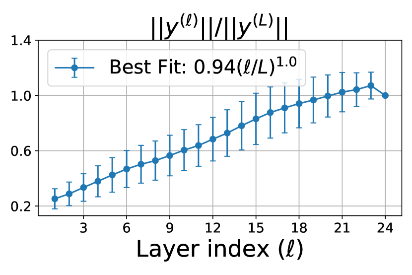
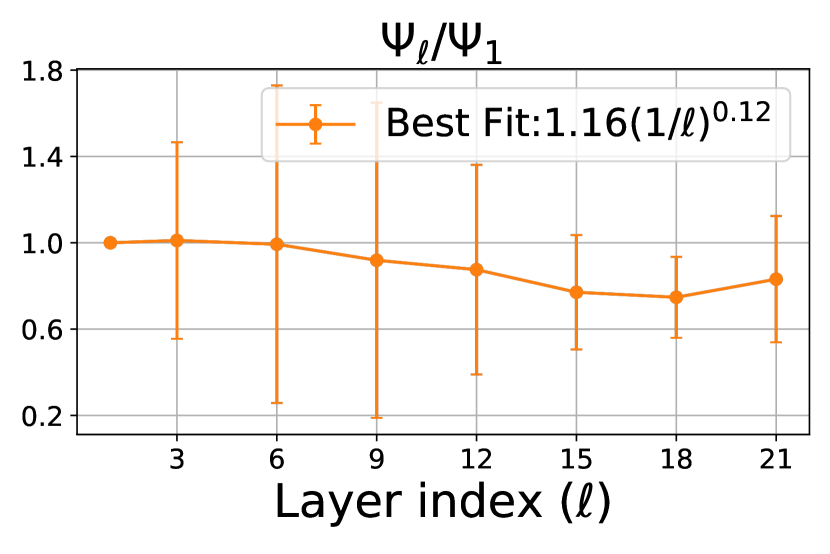
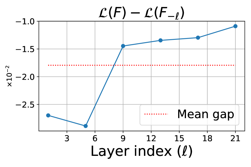
Figure 3: Stability study on BERT-Large trained for $50k$ steps by RaPTr with subnetworks of length $L-1$. Left to right: Behavior of (a) norms of intermediate activations ${\bm{y}}^{(\ell)}$, (b) $\Psi_{\ell}/\Psi_{1}$ (Definition 5.2), and (c) Loss gap between different random subnetwork $F_{-\ell}$ and model $F$, given by $\mathcal{L}(F)-\frac{1}{L}\sum_{\ell=1}^{L}\mathcal{L}(F_{-\ell})$. Key observations: (a) Norms of the intermediate activations grow linearly with $\ell$, (b) $\Psi_{\ell}$ changes slowly with $\ell$ as $(\frac{L}{\ell})^{0.12}$, suggesting a worse-case bound of $\mathcal{O}(L^{-0.88})$ on $\mathcal{L}(F)-\frac{1}{L}\sum_{\ell=1}^{L}\mathcal{L}(F_{-\ell})$ based on Theorem 5.3 (c) Interestingly, $\mathcal{L}(F)\leq\frac{1}{L}\sum_{\ell=1}^{L}\mathcal{L}(F_{-\ell})$, even when model is trained with $L-1$ random subnetworks.

We summarize the key takeaways and recommendations from our experimental findings on BERT and UL2 below. Overall RaPTr can speed up training by 20-33% and also get better downstream performance, without needing extensive tuning of the stage schedules.

Schedule selection. Overall we find RaPTr to be fairly robust to schedule selections (see Table 6). For practical purposes, we recommend to restrict the number of RaPTr phases to $4$. In the initial phase of the RaPTr, random subnetworks of size $L/2$ are selected, with the size of these subnetworks incrementally increasing at each stage transition until the full model is trained in the final phase. For UL2 training, we find that an initial phase of full model training helps RaPTr. We attribute this to the fast drop in loss that large models can achieve initially, but this deserves more exploration. Furthermore, fixing the first and last layer fixed during training helps.

Learning rate schedule. Keeping the learning rate constant in all phases except the final phase, and decaying the learning rate in the full model training phase helps RaPTr on BERT. However, for UL2, learning rate decay from start is also effective and outperforms baseline training.

Few-epoch settings. RaPTr and other efficient training methods especially help in few-epoch/pass settings (e.g. LLM training), but the gap diminishes with more epochs, which was also reported in (Kaddour et al., 2023).

Inductive bias. We observe inductive benefits of RaPTr over baseline training, where it achieves better downstream performance at same evaluation loss and lower variance. We believe this deserves more exploration.

5 Theoretical Analysis using layer stability

Figure 4: Train and Evaluation Loss behavior for a BERT-Base model trained with RaPTr for 100k steps. We have $4$ stages with 6-8-10-12 schedule (see Section 4 for details). The boundaries are at 25k, 50k, and 75k. Key observation: the model’s train and evaluation loss change smoothly across stage transitions, indicating stability of the model to RaPTr.

Given the empirical success of RaPTr, we aim to get a deeper understanding of some of its properties in this section. While §3 studies the benefit of progressively increasing complexity in training rather than decreasing, in this section we study an orthogonal question of the stability of training across stage transitions. One intriguing observation about RaPTr is that the training loss decreases quite smoothly when transitioning between two stages (see Figure 4 in appendix). This is a priori surprising, because the discrete shift in how the model is trained in the two stages could, in principle, lead to an arbitrarily large spike in the loss at the transition. This phenomenon suggests that the model trained with smaller subnetworks in an earlier stage is a good initializer for the next stage. In this section we study certain general conditions under which training should proceed smoothly across stages, by introducing the idea of layer stability. The stability analysis, when instantiated for linear networks highlights the importance of two popular architectural choices in Transformer models – residual connections and layer normalization. We now define this idea of layer stability.

5.1 Layer stability

In this section, we restrict our discussion to sequences of length $N=1$; generalization to $N>1$ is fairly easy. We represent $\mathcal{L}:\mathbb{R}^{d}\to\mathbb{R}$ as the training loss of the backbone $F$. For a transformer, the output of the backbone $F$ is passed through a classification head $H:\mathbb{R}^{d}\to\mathbb{R}^{V}$ that returns the logits for the cross entropy loss. A common practice is to include a layer normalization layer that normalizes the output of $F$ before projecting to logits. This makes the loss $\mathcal{L}$ scale-invariant to its input (Ioffe and Szegedy, 2015; Ba et al., 2016), which gives us a favorable stability condition, as any perturbation in the output of $F$ results in a loss perturbation that scales with norm of the output perturbation relative to the norm of the output of $F$. Thus, we make the following assumption.

Assumption 5.1 (Relative-Lipschitzness).

There exists a constant $\mu_{\mathcal{L}}>0$ such that for any input ${\bm{x}}\in\mathbb{R}^{d}$, label ${\bm{y}}$ and perturbation $\eta\in\mathbb{R}^{d}$, $\mathcal{L}$ satisfies $\mathcal{L}({\bm{x}}+\eta,{\bm{y}})-\mathcal{L}({\bm{x}},{\bm{y}})\leq\mu_{\mathcal{L}}\left(\left\|\eta\right\|_{2}/\left\|{\bm{x}}\right\|_{2}\right).$

To understand loss changes across stage boundaries of RaPTr, we consider two stage RaPTr: the first stage trains with subnetwork of length $L-1$ by dropping a single layer at random, and the second stage trains the entire model. Suppose $\mathcal{L}_{1}$ and $\mathcal{L}_{2}$ denote the effective loss functions being minimized in the two stages. The aim is to show that $F$ learned in the first stage by minimizing $\mathcal{L}_{1}$ should also result in small value for $\mathcal{L}_{2}$.

Definition 5.2.

Let $F_{-\ell}$ denote the subnetwork after skipping layer $\ell$. The stability of network output with respect to dropping layer $\ell$ is defined as $\Psi_{\ell}({\bm{x}})=\|F_{-\ell}({\bm{x}})-F({\bm{x}})\|_{2}$.

Our result in Theorem 5.3 shows that $\mathcal{L}_{2}(F)-\mathcal{L}_{1}(F)$ is small if the stability scales slower than the output norm.

Theorem 5.3 (Informal, cf Theorem D.1).

Under assumption 5.1 of loss $\mathcal{L}$, $|\mathcal{L}_{2}(F)-\mathcal{L}_{1}(F)|$ is upper bounded by $(\mu_{\mathcal{L}}/L)\mathbb{E}_{{\bm{x}}\in D}(\sum_{\ell=1}^{L}\Psi_{\ell}({\bm{x}}))/\left\|F({\bm{x}})\right\|_{2}$.

The proof follows by observing that $\mathcal{L}_{1}(F)=\frac{1}{L}\sum_{\ell\in[L]}\mathcal{L}(F_{-\ell})$ and $\mathcal{L}_{2}(F)=\mathcal{L}(F)$. Thus, the losses are close if $F_{-\ell}$ is close enough to $F$ for a random $\ell$. So, the relative stability of the network determines the success of the approach. In Fig. 3, we report the stability of BERT-Large during training. Interestingly, we find that $\mathcal{L}_{2}(F)$ is below $\mathcal{L}_{1}(F)$, even when we train with subnetworks of length $L-1$. However, the question still remains, when is a network stable across the stages of RaPTr. For simplicity, we consider the special case of linear residual networks. We show that layer normalization layers and the residual connection helps maintain the stability of RaPTr.

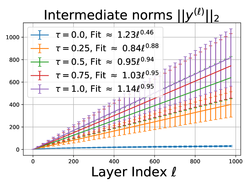
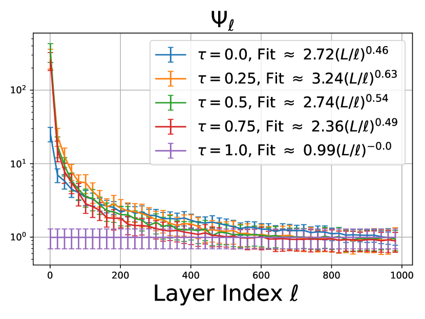
Figure 5: Behavior on a linear residual network with normalization layers with $100$ random samples from $\mathbb{S}^{d-1}$, and dimension $d=100$. The parameters of each layer $\ell$ is represented as $\sqrt{\tau}{\bm{A}}+\sqrt{1-\tau}{\bm{G}}^{(\ell)}$ for a shared matrix ${\bm{A}}\in\mathbb{R}^{d\times d}$ with $\left\|{\bm{A}}\right\|_{2}\leq 1$ and ${\bm{G}}^{(\ell)}\sim\mathcal{N}\left(0,d^{-1/2}{\bm{I}}\right)$. Left to right: Behavior of (a) the norms of intermediate activation ${\bm{y}}^{(\ell)}$ with index $\ell$, (b) $\Psi_{\ell}$ (Definition 5.2) for each stack of layers $F_{\ell:L}$, and (c) $\frac{1}{L}\sum_{\ell=1}^{L}\Psi_{\ell}({\bm{x}})/\left\|F({\bm{x}})\right\|_{2}$ that appears in our bounds in Theorem 5.3.

5.2 Illustrative example: linear networks

We present a more concrete instantiation of Theorem 5.3 for residual network where the layers $f_{1:L}$ are linear with parameters ${\bm{W}}_{1:L}$. The layer output is ${\bm{y}}^{\ell}={\bm{y}}^{(\ell-1)}+{\bm{W}}_{\ell}{\bm{y}}^{(\ell-1)}$ or ${\bm{y}}^{\ell}={\bm{y}}^{(\ell-1)}+{\bm{W}}_{\ell}{\bm{y}}^{(\ell-1)}/\left\|{\bm{y}}^{(\ell-1)}\right\|_{2}$ depending on whether layernorm is enabled or not respectively . We also study another setting with layernorm but no residual connection; so ${\bm{y}}^{\ell}={\bm{W}}_{\ell}{\bm{y}}^{(\ell-1)}/\left\|{\bm{y}}^{(\ell-1)}\right\|_{2}$. For this setting, the following result shows the scale of $\Psi_{\ell}$ and output norm.

Lemma 5.4.

At random initialization where ${\bm{W}}_{i}\sim\mathcal{N}(0,d^{-1/2}{\bm{I}})$, for a randomly sampled ${\bm{x}}\in\mathbb{S}^{d-1}$, we have

1. With residual connection & layernorm, $\Psi_{\ell}({\bm{x}})=\mathcal{O}(\sqrt{L/\ell})$ & $\left\|F({\bm{x}})\right\|_{2}=\Omega(\sqrt{L})$. Then the gap in losses between stages is $\mathcal{O}(1/\sqrt{L})$.

2. Without residual connection, $\Psi_{\ell}({\bm{x}})=\Omega(1)$ & $\left\|F({\bm{x}})\right\|_{2}=\mathcal{O}(1)$. Thus the gap in losses between stages is $\Omega(1)$.

3. Without layernorm, we have $\Psi_{\ell}({\bm{x}})=\Omega(2^{(L-1)/2})$ and $\left\|F({\bm{x}})\right\|_{2}=\mathcal{O}(2^{L/2})$ . Thus the gap in losses between stages is $\Omega(1)$.

In the Appendix, we show similar results for perfectly aligned layers, where layer parameters are equal to ${\bm{A}}$ (Lemma D.3). These examples capture the cases of perfectly correlated and uncorrelated layers. We can consider even more general scenarios, where the layers parameters are expressed as combination of a Gaussian and a shared matrix (Fig. 5). We run simulations and observe that for each $\tau$, $\Psi_{\ell}=\mathcal{O}(L/\ell)^{0.5}$ , while the output norm grows faster as $\Omega(L^{0.5})$ . Then, the gap between a $L-1$ random subnetwork and the full model scales as $\mathcal{O}(L^{-0.4})$.

6 Related works

The literature on training deep networks is vast; thus, we mainly focus on the most relevant works.

Stagewise efficient pretraining. Stacking has been further extended to other dimensions (e.g. width) by (Gu et al., 2020), (Shen et al., 2022), (Wang et al., 2023), and (Gesmundo and Maile, 2023) in the form of growth operators ensuring the loss is preserved while growing the network. While we mainly focused on model depth expansion, other growth operators also have an analog in our subnetwork training framework and are left for future work.

Stochastic depth. RaPTr bears some similarity to stochastic depth —structured dropout that drops layers at random with fixed probability during training to train extremely deep residual networks without increasing the training cost (Huang et al., 2016). A key distinction is that the probability of dropping layers is fixed during training and can thus be viewed as a regularization (Pham et al., 2019; Steiner et al., 2021; Tolstikhin et al., 2021; Liu et al., 2023c), which is different from the role dropout plays in our work. Additionally (Fan et al., 2019) use fixed stochastic depth to select lower depth subnetworks for inference efficiency rather than training efficiency.

Subnetwork training. Training of random paths and subnetworks has been used in other contexts, e.g. parameter efficient fine-tuning (Houlsby et al., 2019; Pfeiffer et al., 2021; Hu et al., 2022; Liu et al., 2022) to reduce memory footprint, distributed and federated training (Dun et al., 2022) using multiple machines, and incremental learning (Jathushan et al., 2019) to avoid forgetting in continual learning. These ideas are not motivated by or used for reducing FLOPs during pretraining, to the best of our knowledge.

Residual networks as ensembles. Training with random paths can be weakly viewed as ensembles over paths, and the connection between ResNets (He et al., 2016) and ensembles of shallow networks was first point out in Veit et al. (2016) for vision models. (Dong et al., 2021) showed the same phenomenon for self-attention models, where longer paths lead to rank-collapse in the self-attention module. (Chang et al., 2023) study vision transformers (Dosovitskiy et al., 2020) as a cascade of multiple paths and propose pruning and self-distillation to remove long paths and improve performance. All these works mainly provide a novel perspective or inference efficiency but do not focus on training efficiency.

Learnable scaling of residual blocks. (Bachlechner et al., 2021), (Zhang et al., 2019), (Touvron et al., 2021) consider learnable scales on the output of the residual blocks. These works aim to understand favorable initialization of the learnable scales under various constraints for faster training, which is very different from the role of scaling in our algorithm.

Early exit for efficient inference

A lot of recent works have focused on improving inference efficiency for large language models.  (Lei et al., 2023; Tay et al., 2022; Del Corro et al., 2023; Xin et al., 2020; Zhou et al., 2020; Hou et al., 2020). However, none of these works focus on efficient fine-tuning. (Lei et al., 2023) modified pre-training by substituting resource-intensive MLP computations with straightforward classifiers for a predetermined fraction of tokens within the sequence. It’s worth noting that their primary focus was on accelerating inference time rather than enhancing the efficiency of the pre-training process.

7 Conclusion and Future Work

This work proposes a stagewise training framework of progressive subnetworks for efficient pretraining, and evaluates a natural instantiation of this framework (RaPTr) based on training random paths/subsets of layers. Overall RaPTr yields better quality language models than baseline training, while reducing the total FLOPs by at least 20-30%. At the same speedup, it is also better than prior layer dropping and stacking based approaches. There are other stacking approaches with different growth functions in the literature (see §6 for references), and exploring analogs of subnetwork training for these growth functions could be a fruitful direction. From theory perspective, the current analysis provides insights into why the loss is stable at stage boundaries, but it does not explain the stronger empirical finding that the loss decreases at transitions. Additionally, there is evidence of certain desirable inductive biases of RaPTr style training, e.g., better downstream performance, smaller variance, which are not explained by our analysis. A better understanding of these phenomena could inspire other efficient training algorithms.

Broader Impact

Training LLMs demands extensive computational resources and infrastructure. Our paper proposes an algorithm that aims to accelerate their pre-training. Accelerating the training of large language models (LLMs) can significantly reduce their environmental impact by lowering energy consumption and minimizing carbon footprints. Optimizations in algorithms and infrastructure will lead to more efficient use of computational resources and will promote sustainability of the field of AI.

Furthermore, we observe benefits of structured pre-training (simple-to-complex) of these models on downstream tasks. Hopefully, these ideas can lead to better pre-training strategies for LLMs.

Table 5: Additional rows from Table 3: we compare baseline runs at two learning rate schedules, and run compare RaPTr and Gradual stacking with a new 6-12-18-24 schedule. Key Observations: (a) Cosine decay learning works best for the baseline, compared to Square-root schedule proposed by [Tay et al., 2022], (b) The performance of gradual stacking improves with the new schedule, implying a performance dependence with appropriate scheduling, and (c) RaPTr’s performance doesn’t change much with the new schedule.

	Rel. FLOPs	Eval Loss	Trivia QA	Tydi QA	SQuADv2	SGLUE	Average
Baseline (Square-root LR decay)	1.2	2.07	23.4	31.9	44.3	60.0	39.9
Baseline (Cosine LR decay)	1.2	2.06	25.0	34.4	42.1	60.0	40.4
Equiflop Baseline (Square-root LR decay)	1	-	32.1	22.1	-	60.9	38.4
Equiflop Baseline (Cosine LR decay)	1	2.07	24.3	35.7	42.37	60.6	40.7
6-12-18-24 Stacking	1	2.06	22.1	34.6	38.0	60.5	38.8
12-16-20-24 Stacking	1	2.08	20.1	28.6	36.0	60.4	36.3
12-16-20-24 RaPTr	1	2.08	22.2	38.2	40.6	60.1	40.3
(+30k initial full-model train)	1	2.06	25.8	36.7	44.1	60.9	41.9
6-12-18-24 RaPTr
(+30k initial full-model train)	1	2.06	24.2	37.3	42.3	61.1	41.2

Appendix A Additional Experiment details

A.1 Details on PLD

The progressive layer dropping algorithm [Zhang and He, 2020] is given in Algorithm 2. PLD employs a time and depth schedule that determines the probability of dropping each block. The time schedule begins with a zero probability of dropping each block. Then it increases this probability throughout the training process until it reaches a maximum of $(1-\bar{\alpha})$, where the hyperparameter $\bar{\alpha}=0.5$. We vary $\bar{\alpha}$ depending on the average FLOP perplexity we want to achieve in the end. With $\bar{\alpha}=p$, the FLOPs reduce by $1-(p/2)$.

The depth schedule ensures that blocks located earlier in the model are dropped with a lower probability than those located later/deeper. An important hyperparameter of the depth schedule in PLD is $\gamma_{f}$, which controls the rate at which the probability of dropping layers increases. A higher value of $\gamma_{f}$ leads to a quicker increase in the probability. Zhang and He [2020] set $\gamma_{f}$ to 100 in their experiments.

A.2 Details for polynomial training

We present in Figure 2 the results from a 20-layer residual network trained on 100-dimensional data. Our $f^{\star}$ has max degree $k=10$ restricted to the first $t=20$ variables (${\bm{x}}_{1:20}$) in the input. We pick $m=20$ random basis polynomials for each degree $\ell\leq 10$. We set the average drop rate of PLD to $\bar{\alpha}=0.6$, such that the average FLOPs is $80\%$ lower to a baseline run. For RaPTr, we use $4$-stage training, with the stages represented by its $(p,\mathcal{I})$ as $(0.4,\{\}),(0.6,\{\}),(0.8,\{\}),$ and$(1.0,\{\})$ respectively. The lengths of each stage have been set as $16.5k$, $16.5k$, $16.5k$, and $48.5k$ respectively, such that the average FLOPs is $80\%$ lower to a baseline run (please see Appendix B).

A.3 Details for BERT

Equal step Pretraining

The batch-size is set to $256$ and $512$ for BERT-Base and BERT-Large respectively. Following J. Reddi et al. [2023], we use a learning rate warmup of 10k steps and keep learning rate constant in all phases, followed by a linear learning rate decay to $0$ in the final full model training phase. We set the peak learning rate as $10^{-4}$ in all our experiments.

Equivalent flop Pretraining

To make a fair comparison across all methods, we tune the peak the learning rate in the grid $\{1,1.6,2.5,4\}\times 10^{-4}$ for BERT-Base and grid $\{1,1.6,2.5\}\times 10^{-4}$ for BERT-Large in all settings.

Finetuning

We fine-tune BERT models for $3$ epochs with batch-size $32$, using a learning rate grid search over $\{1,2,3,5\}\times 10^{-5}.$ We use a linear warmup schedule over initial $6\%$ training steps, followed by constant learning rate schedule for the rest of the training.

Algorithm 2 Progressive layer dropping (PLD) [Zhang and He, 2020]

1:  Input: iterations $T$, layer keep probability $\bar{\alpha}$, temperature budget $\gamma_{f}>0$, layers $L$, functions (self-attention, layer-norm, feed-forward) $f_{ATTN},f_{LN},f_{FFN}$, loss function $\mathcal{L}$, data $(\mathbf{x}_{0},\mathbf{y})$, output layer $f_{O}$

2:  $\gamma\leftarrow\frac{\gamma_{f}}{T}$

3:  for $t$ $\leftarrow$ 1 to $T$ do

4:     $p\leftarrow 1$ {Keep probability.}

5:     $\alpha_{t}\leftarrow(1-\bar{\alpha})\exp(-\gamma\cdot t)+\bar{\alpha}$

6:     $p_{d}\leftarrow\frac{1-\alpha_{t}}{L}$ {Layer decay.}

7:     for $i$ $\leftarrow$ 0 to $L-1$ do

8:        $s\sim\operatorname{Bernoulli}(p)$ {Keep or drop.}

9:        if $s==0$ then

10:           $\mathbf{x}_{i+1}\leftarrow\mathbf{x}_{i}$ {Drop.}

11:        else

12:           $\mathbf{x}_{i}^{\prime}\leftarrow\mathbf{x}_{i}+\frac{f_{ATTN}(f_{LN}(\mathbf{x}_{i}))}{p}$

13:           $\mathbf{x}_{i+1}\leftarrow\mathbf{x}_{i}^{\prime}+\frac{f_{FFN}(f_{LN}(\mathbf{x}_{i}^{\prime}))}{p}$

14:        end if

15:        $p\leftarrow p-p_{d}$ {Decay prob.}

16:     end for

17:     $\ell\leftarrow\mathcal{L}(f_{O}(\mathbf{x}_{L}),\mathbf{y})$

18:     $f_{ATTN},f_{LN},f_{FFN},f_{O}\leftarrow\operatorname{Update}(\ell)$

19:  end for

A.4 Details for UL2

Pretraining

Similar to our experiments on BERT, we use a linear warmup of $10$K steps, followed by constant learning rate in all stages, and a cosine decay to $0.1\times$ the peak learning rate in the final full model training stage. The peak learning rate is set to $10^{-2}$.

Reported datasets in Table 3 include Trivia QA [Joshi et al., 2017], Tydi QA [Clark et al., 2020], SQuADV2 [Rajpurkar et al., 2018], and SuperGLUE [Wang et al., 2019]. For QA tasks, we report Exact match scores, and report average accuracy for SuperGLUE tasks. To reduce variance, we report average performance across $3$ runs for the most representative setting for each method. We conduct extensive downstream evaluation of the trained models from Table 3 on additional downstream tasks and under higher shot in-context setting. Additional tasks include QA tasks like natural QA [Kwiatkowski et al., 2019], web QA [Berant et al., 2013], DROP [Dua et al., 2019], CoQA [Reddy et al., 2019], and QuAC [Choi et al., 2018]; and completion tasks like Storyclose [Mostafazadeh et al., 2017], Hellaswag [Zellers et al., 2019], and LAMBADA [Paperno et al., 2016].

Boundaries for 12-16-20-24 RaPTr and Gradual Stacking are 40k, 120k, and 240k (decided using Appendix B). The average subnetwork length used during training turns out to be $20$ with this schedule. When we introduce an initial 30k full-model training for RaPTr, we shift the boundaries by 30k so that the average subnetwork length stays $20$.

Additional Pretraining experiments

In Table 5, we have the following additional runs compared to Table 3 in the main paper.

Baseline learning rate schedule: We first compare standard training with cosine decay learning rate to a standard training run with Square-root learning rate decay that was used in the original paper [Tay et al., 2022]. We observe that the model with square-root learning rate performs significantly worse compared to the model with cosine decay learning rate. Hence, we use standard training with cosine decay learning rate as our baseline.

Stacking dependence on schedule: Secondly, we try another schedule for Gradual Stacking, which contains 4 stages and is represented by 6-12-18-24. The stage lengths have been adjusted such that the average number of layers used over training is $20$. We set the stage boundaries as 17k, 74k, and 172k respectively. We observe that 6-12-18-24 Gradual Stacking performs much better than 12-16-20-24 Gradual Stacking on various downstream tasks. This signals towards the dependency of Gradual Stacking on proper schedule selection.

On the other hand RaPTr doesn’t show a big difference with 6-12-18-24 schedule, when compared to 12-16-20-24 schedule. A proper analysis of both the methods on schedule dependencies is kept for future work.

Appendix B Schedule selection

We follow two schedules from [J. Reddi et al., 2023], Equal and Proportional, to build the lengths of each stage in RaPTr and Stacking. For Equal scheduling, used in Tables 1 and 2, we split training into $k$ equal stages. For Proportional scheduling in Table 3, we increase the length of a stage in proportion to index of the stage. For example, for 12-16-20-24 RaPTr and Stacking with proportional scheduling for $400k$ training steps, the stage lengths are set as $40k$, $80k$, and $120k$ respectively.

The flop counts are decided on the basis of average subnetwork length during training. For example, if the average subnetwork length is $18$ for a model with $24$ layers, we consider relative flops of RaPTr compared to baseline as $0.75$.

For 12-16-20-24 RaPTr with Equal schedule, the average subnetwork length during training is given by $18$, while for Proportional schedule, the average subnetwork length during training is given by $20$. However, when either Equal and Proportional schedules don’t return the target average subnetwork length, we re-consider the stage lengths by taking the closest candidate among Equal and Proportional schedules and remove equal steps from each of the first $k-1$ stages and add to the final full model training stage. For example, in Table 5, with 6-12-18-24 RaPTr and target average subnetwork length $20$, Proportional schedule returns an average subnetwork length of $18$ and stage lengths $40k$, $80k$, $120k$ and $160k$ respectively. We then aim to find $x$ such that stage lengths of $40k-x$, $80k-x$, $120k-x$ and $160k+3x$ returns the desired average subnetwork length. On solving for $x$, we get $x=22k$.

B.1 Ablation on different schedules for BERT-Base

We conduct experiments on RaPTr with different stage schedules that have same relative flop counts in Table 1. We observe on BERT-Base that different schedules differ by atmost $0.01$ in pre-training loss and $0.1-0.5$% in downstream performance on average. Thus, we conclude that RaPTr is robust to the stage schedule selection.

For UL2, we use the following stage schedules to minimize computational overhead. We restrict the number of phases in RaPTr to $4$. The first stage selects a sub-network with half of the layers at random at each step. We increase the sub-network size by an equal quantity in each stage transition, such that we train the full model in the final phase.

Table 6: Performance of RaPTr on BERT-Base with different schedules. The average subnetwork size for each schedule is $9$, which makes each schedule $1.33$x faster than the baseline model (provided for reference). We use the same hyperparameters as used in Table 1. We observe minor differences between different schedules, indicating robustness of RaPTr.

RaPTr schedule	Rel. flops	Eval loss	MNLI	QNLI	SST-2	Avg.
3-6-9-12	1	1.76	82.0	89.6	92.0	87.9
4-8-12	1	1.76	81.9	89.3	91.5	87.6
6-9-12	1	1.75	82.3	89.2	91.0	88.0
6-8-10-12	1	1.75	82.1	89.8	92.4	88.1
Baseline	1.33	1.76	81.5	90.5	91.4	87.8

B.2 Ablation on fixed layer set $\mathcal{I}$ for BERT-Base

We conduct experiments on 6-8-10-12 RaPTr on BERT-Base with different fixed layer set $\mathcal{I}$ (Table 7). We observe that fixed set selection of $\{1,12\}$ performs the best among other candidates. This selection however can be expensive to verify for other settings like UL2. Hence, in all subsequent experiments, we continue with the first and last layer fixed in all stages of RaPTr.

Table 7: Performance of RaPTr on BERT-Base with different $\mathcal{I}$ set for 6-8-10-12 RaPTr run for $100k$ steps. We use the same hyperparameters as used in Table 1, except the training steps reduced to $100k$ steps. We observe that fixing the first and the last layer at all times lead to slightly better performance, compared to other candidates.

$\mathcal{I}$ set	Eval loss	MNLI	QNLI	SST-2	Avg.
$\{\}$	2.12	-	-	-	-
$\{1\}$	2.13	-	-	-	-
$\{1,12\}$	2.11	78.6	86.77	88.69	84.7
$\{1,2,12\}$	2.13	-	-	-	-
$\{1,11,12\}$	2.12	77.4	87.0	89.4	84.6
$\{1,2,11,12\}$	2.14	78.0	86.1	88.8	84.3
$\{1,2,3,11,12\}$	2.18	77.4	86.5	88.4	84.1
$\{1,2,10,11,12\}$	2.16	-	-	-	-

Appendix C System speed of different subnetworks

We report the speed of training in steps/sec for UL2 models with different subnetwork sizes on TPU 16x16 chips with percore batch size of $2$ in Table 8. Suppose $t$ is the total time for $400k$ steps with a 24-layer model in UL2 training. In Table 3, we use 12-16-20-24 RaPTr that has $20\%$ ”theoretical” flop count reduction, with the stage lengths given by $40k$, $80k$, $120k$, and $240k$ respectively (Appendix B). Theoretically, the necessary time required should be $0.83t$. Using the training speed numbers of Table 8, it takes approximately $0.84t$ to complete $400k$ steps with RaPTr on our machine, close to the theoretical training time.

Table 8: Training Steps/sec at different stages on 24-layer UL2

subnetwork size	steps/sec
12	2.0
16	1.6
20	1.4
24	1.1

Appendix D Noise stability for transformers

Theorem D.1.

Suppose $\mathcal{L}$ satisfies the following condition $\mathcal{L}$ satisfies the following condition for any input $\tilde{{\bm{x}}},\eta\in\mathbb{R}^{d}$ and label ${\bm{v}}\in\{0,1\}^{V}$ for some constant $\mu_{loss}$ :

$$\mathcal{L}(\tilde{{\bm{x}}}+\eta,{\bm{v}})-\mathcal{L}(\tilde{{\bm{x}}},{\bm{v}})\leq\mu_{\mathcal{L}}\frac{\left\|\eta\right\|_{2}}{\left\|\tilde{{\bm{x}}}\right\|_{2}}.$$ (3)

The difference between expected loss of $(L-1)$-RaPTr and $L$-RaPTr, i.e. $|\mathcal{L}_{2}(F)-\mathcal{L}_{1}(F)|$, is upper bounded by $\frac{C}{L}\mathbb{E}_{{\bm{x}}\in D}(\sum_{\ell=1}^{L}\Psi_{\ell}({\bm{x}}))/\left\|F({\bm{x}})\right\|_{2}$ for some constant $C$ that depends on regularity properties of the head $H$ on top of the backbone $F$.

Proof of Theorem 5.3.

Denote by $F_{-\ell}$ the $L$ candidates that we can randomly choose from during $L-1$ RaPTr training. The output of $F_{-\ell}$ on any input ${\bm{x}}$ is equivalent to the output of the model $F$ on ${\bm{x}}$ and $\alpha_{1:L}$, with $\alpha_{\ell}=0$ and the rest set to $1$.

Then, the average loss of $L-1$ random training is given by

$$\mathcal{L}_{2}(F)=\frac{1}{L}\sum_{i=1}^{L}\mathbb{E}_{{\bm{x}},{\bm{y}}\sim D}\mathcal{L}\left(F_{-\ell}({\bm{x}}),{\bm{v}}\right).$$

On the other hand, the loss of the full model is given by

$$\mathcal{L}_{1}(F)=\mathbb{E}_{{\bm{x}},{\bm{v}}\sim D}\mathcal{L}\left(F({\bm{x}}),{\bm{v}}\right).$$

Hence, the expected difference between loss of $L-1$ random training and full model is given by

$$\mathcal{L}_{2}(F)-\mathcal{L}_{1}(F) =\frac{1}{L}\sum_{i=1}^{L}\mathbb{E}_{{\bm{x}},{\bm{v}}\sim D}\left(\mathcal{L}\left(F_{-\ell}({\bm{x}}),{\bm{v}}\right)-\mathcal{L}\left(F({\bm{x}}),{\bm{v}}\right)\right)$$

$$\leq\frac{1}{L}\sum_{i=1}^{L}\mathbb{E}_{{\bm{x}},{\bm{v}}\sim D}\quad\mu_{\mathcal{L}}\frac{\left\|F_{-\ell}({\bm{x}})-F({\bm{x}})\right\|_{2}}{\left\|F({\bm{x}})\right\|_{2}}$$

$$\leq\frac{1}{L}\sum_{i=1}^{L}\mathbb{E}_{{\bm{x}},{\bm{v}}\sim D}\quad\mu_{\mathcal{L}}\frac{\psi_{\ell}}{\left\|F({\bm{x}})\right\|_{2}}.$$

Here the pre-final step uses the definition of $\mu_{\mathcal{L}}$ from Equation 3, and the final step uses the definition of $\Psi_{\ell}$ from Definition 5.2. ∎

Discussion

An example of a loss function with bounded $\mu_{\mathcal{L}}$ is a transformer model, that uses a layer normalization layer before using an embedding matrix $\Phi$ to compute the logits. The logits are then compared with the true label with a cross-entropy loss with a softmax function on logits. $\mu_{\mathcal{L}}$ hence depends on the $\ell_{2}$ norm of $\Phi$ and the weight parameters of the layer normalization layer.

D.1 Noise stability of linear residual networks

We first report a random matrix lemma that we will repeatedly use in this section.

Lemma D.2 (Norm of the output after a random linear layer, lemma 7.1 in [Allen-Zhu et al., 2019] without activation function).

For any $\epsilon>0$, a random matrix ${\bm{A}}\sim\mathcal{N}(0,d^{-1/2})$ and a randomly sampled input ${\bm{x}}\in\mathbb{S}^{d-1}$, w.p. atleast $1-e^{-\Omega(d\epsilon^{2})}$,

$$(1-\mathcal{O}(\epsilon))\leq\left\|{\bm{A}}{\bm{x}}\right\|_{2}\leq(1+\mathcal{O}(\epsilon)).$$

We repeat Lemma 5.4 from the main paper. See 5.4

Proof of Lemma 5.4.

We outline the proof for each case.

1. With residual connection and layer normalization, the function $F$ computes the intermediate activations ${\bm{y}}^{(1)},\cdots,{\bm{y}}^{(L)}$ on an input ${\bm{x}}$ as follows.

   $${\bm{y}}^{(\ell)}=\left({\bm{I}}+\frac{{\bm{W}}_{\ell}}{\left\|{\bm{y}}^{(\ell-1)}\right\|}\right){\bm{y}}^{(\ell-1)}.$$

   Similar to Lemma D.2, we can show w.h.p. with respect to the randomness of ${\bm{W}}_{1},\cdots,{\bm{W}}_{L}$, for all $\ell\leq L$, $\sqrt{\ell}(1-\mathcal{O}(1))\leq\left\|{\bm{y}}^{(\ell)}\right\|_{2}\leq\sqrt{\ell}(1+\mathcal{O}(1)).$

   Ignoring the error terms, we can simply write

   $${\bm{y}}^{(\ell)}=\left({\bm{I}}+\frac{{\bm{W}}_{\ell}}{\sqrt{\ell}}\right){\bm{y}}^{(\ell-1)}.$$

   Pick a general layer $\ell$ to be dropped. Then,

   $$F_{-\ell}({\bm{x}})-F({\bm{x}})=\prod_{\ell^{\prime}=\ell+1}^{L}\left(1+\frac{{\bm{W}}_{\ell^{\prime}}}{\sqrt{\ell^{\prime}}}\right)\frac{{\bm{W}}_{\ell}}{\sqrt{\ell}}{\bm{y}}^{(\ell-1)}+err,$$

   where the $err$ term appears because of the change in scales of activations ${\bm{y}}^{(\ell+1)},\cdots,{\bm{y}}^{(L)}$ with the dropping of layer $\ell$. This error can be bounded as $\mathcal{O}(\sqrt{L}/\ell)$ using the same procedure followed below to bound the first term on R.H.S..

   Similar to bounding the norms of ${\bm{y}}^{(\ell)}$, w.h.p. we can show that

   $$\left\|\prod_{\ell^{\prime}=\ell+1}^{L}\left(1+\frac{{\bm{W}}_{\ell^{\prime}}}{\sqrt{\ell^{\prime}}}\right)\frac{{\bm{W}}_{\ell}}{\sqrt{\ell}}{\bm{y}}^{(\ell-1)}\right\|_{2}\leq\sqrt{\frac{L}{\ell}}.$$

   Hence,

   $$\psi_{\ell}:=\left\|F_{-\ell}({\bm{x}})-F_{\ell}({\bm{x}})\right\|_{2}\leq\mathcal{O}(\sqrt{L/\ell}).$$

   This implies

   $$\frac{1}{L}\sum_{\ell}\psi_{\ell}({\bm{x}})=\frac{1}{L}\sum_{\ell}\mathcal{O}(\sqrt{L/\ell})=\mathcal{O}(1).$$

   Since the gap in $\mathcal{L}_{2}$ and $\mathcal{L}_{1}$ is bounded by $\mathcal{O}(\mathbb{E}_{{\bm{x}}}\frac{1}{L}\sum_{\ell}\psi_{\ell}({\bm{x}})/||F({\bm{x}})||)$ from Theorem 5.3, we have the gap as $\mathbf{O}\left(\frac{1}{\sqrt{L}}\right)$.

2. With no normalization, the function $F$ looks as follows.

   $${\bm{y}}^{(\ell)}=\left({\bm{I}}+{\bm{W}}_{\ell}\right){\bm{y}}^{(\ell-1)}.$$

   Similar to Lemma D.2, we can show w.h.p. with respect to the randomness of ${\bm{W}}_{1},\cdots,{\bm{W}}_{L}$, for all $\ell\leq L$, $2^{\ell/2}(1-\mathcal{O}(1))\leq\left\|{\bm{y}}^{(\ell)}\right\|_{2}\leq 2^{\ell/2}(1+\mathcal{O}(1)).$

   With a drop in layer, we get

   $$F_{-\ell}({\bm{x}})-F({\bm{x}})=\prod_{\ell^{\prime}=\ell+1}^{L}\left({\bm{I}}+{\bm{W}}^{\ell^{\prime}}\right){\bm{W}}_{\ell}\prod_{\ell^{\prime}=1}^{\ell-1}\left({\bm{I}}+{\bm{W}}^{\ell^{\prime}}\right){\bm{x}}.$$

   Similar to Lemma D.2, we can show w.h.p. with respect to the randomness of ${\bm{W}}_{1},\cdots,{\bm{W}}_{L}$, $\left\|\prod_{\ell^{\prime}=\ell+1}^{L}\left({\bm{I}}+{\bm{W}}^{\ell^{\prime}}\right){\bm{W}}_{\ell}\prod_{\ell^{\prime}=1}^{\ell-1}\left({\bm{I}}+{\bm{W}}^{\ell^{\prime}}\right){\bm{x}}\right\|_{2}\geq\mathcal{O}(2^{(\ell-1)/2}).$

   This implies $\left\|F_{-\ell}({\bm{x}})-F({\bm{x}})\right\|_{2}=\Omega(2^{(\ell-1)/2}).$

   The argument can now be completed by using Theorem 5.3.

3. Without residual connection, the function $F$ looks as follows.

   $${\bm{y}}^{(\ell)}={\bm{W}}_{\ell}\frac{{\bm{y}}^{(\ell-1)}}{\left\|{\bm{y}}^{(\ell-1)}\right\|_{2}}.$$

   Similar to Lemma D.2, we can show w.h.p. with respect to the randomness of ${\bm{W}}_{1},\cdots,{\bm{W}}_{L}$, for all $\ell\leq L$, $(1-\mathcal{O}(1))\leq\left\|{\bm{y}}^{(\ell)}\right\|_{2}\leq(1+\mathcal{O}(1)).$ Thus, ignoring error terms, the network $F$ roughly looks like

   $${\bm{y}}^{(\ell)}={\bm{W}}_{\ell}{\bm{y}}^{(\ell-1)}.$$

   With a drop in layer, we get

   $$F_{-\ell}({\bm{x}})-F({\bm{x}})=\prod_{\ell^{\prime}=\ell+1}^{L}{\bm{W}}_{\ell^{\prime}}({\bm{W}}^{(\ell)}-{\bm{I}})\prod_{\ell^{\prime}=1}^{\ell-1}{\bm{W}}_{\ell^{\prime}}{\bm{x}}.$$

   Using randomness of ${\bm{W}}^{(\ell)}$ this can be shown to be of norm $\Omega(1)$. The argument can now be completed by using Theorem 5.3.

∎

We show a similar lemma for the case where all the matrices ${\bm{W}}_{i}$ are identical to a matrix ${\bm{A}}$.

Lemma D.3.

When the layers are perfectly aligned, i.e. all weights ${\bm{W}}_{i}={\bm{A}}$ for some matrix ${\bm{A}}$ with $\left\|{\bm{A}}\right\|_{2}=1$ and for simplicity, assume second eigenvalue $\lambda_{2}({\bm{A}})=1-\delta$ for some $\delta>0$, we have for a randomly sampled ${\bm{x}}\in\mathbb{S}^{d-1}$

1. With residual connection & layernorm, we have $\Psi_{\ell}({\bm{x}})=\mathcal{O}(1)$ and $\left\|F({\bm{x}})\right\|=\Omega(L)$. Thus, the gap in losses between stages is $\mathcal{O}(1/L)$.

2. Without residual connection, we have both $\Psi_{\ell}({\bm{x}})=\mathcal{O}(\delta^{-1}e^{-\ell})$ and $\left\|F({\bm{x}})\right\|=\mathcal{O}(1)$. Thus the gap in losses between stages is $\mathcal{O}(\frac{1}{L})$.

3. Without layernorm, we have $\Psi_{\ell}({\bm{x}})=\Omega(2^{L-1})$ and $\left\|F({\bm{x}})\right\|=\mathcal{O}(2^{L})$ . Thus the gap in losses between stages is $\Omega(1)$.

Proof of Lemma D.3.

We outline the proof for each case.

1. With residual connection & layernorm, the function $F$ computes the intermediate activations ${\bm{y}}^{(1)},\cdots,{\bm{y}}^{(L)}$ on an input ${\bm{x}}$ as follows.

   $${\bm{y}}^{(\ell)}=\left({\bm{I}}+\frac{{\bm{A}}}{\left\|{\bm{y}}^{(\ell-1)}\right\|}\right){\bm{y}}^{(\ell-1)}.$$

   We show that the above method will behave like power method, i.e. ${\bm{y}}^{(\ell)}$ will be of magnitude $\Omega(\ell)$ and will be $\epsilon$-close in angle to the top eigenvector of ${\bm{A}}$, denoted as ${\bm{v}}_{1}({\bm{A}})$, provided $\ell\geq\Omega((1/\delta)\log(1/\epsilon)).$

   We give an inductive argument as follows. Consider any layer $\ell$. Say $\theta_{\ell}$ denotes the angle between ${\bm{y}}^{(\ell)}$ and ${\bm{v}}_{1}({\bm{A}})$. Also, say $\Pi^{\perp}_{{\bm{v}}1}$ denotes an orthogonal projection to subspace spanned by the rest of the eigenvectors of ${\bm{A}}$. Then,

   $$\left|\tan\theta_{\ell+1}\right| =\frac{\left|\langle{\bm{v}}_{1}({\bm{A}}),{\bm{y}}^{(\ell+1)}\rangle\right|}{\left\|\Pi^{\perp}_{{\bm{v}}1}({\bm{y}}^{(\ell+1)})\right\|_{2}}$$

   $$=\frac{\left|\langle{\bm{v}}_{1}({\bm{A}}),{\bm{y}}^{(\ell)}\rangle+\langle{\bm{v}}_{1}({\bm{A}}),{\bm{A}}{\bm{y}}^{(\ell)}\rangle\right|}{\left\|\Pi^{\perp}_{{\bm{v}}1}({\bm{y}}^{(\ell)})+\Pi^{\perp}_{{\bm{v}}1}{\bm{A}}{\bm{y}}^{(\ell)}\right\|_{2}}$$

   $$=\frac{2\left|\langle{\bm{v}}_{1}({\bm{A}}),{\bm{y}}^{(\ell)}\rangle\right|}{\left\|\Pi^{\perp}_{{\bm{v}}1}({\bm{y}}^{(\ell)})+\Pi^{\perp}_{{\bm{v}}1}{\bm{A}}{\bm{y}}^{(\ell)}\right\|_{2}}$$

   $$\leq\frac{2\langle{\bm{v}}_{1}({\bm{A}}),{\bm{y}}^{(\ell)}\rangle}{\left\|\Pi^{\perp}_{{\bm{v}}1}({\bm{y}}^{(\ell)})+\lambda_{2}({\bm{A}})\Pi^{\perp}_{{\bm{v}}1}{\bm{y}}^{(\ell)}\right\|_{2}}$$

   $$=\frac{2}{1+\lambda_{2}({\bm{A}})}\left|\tan\theta_{\ell}\right|.$$

   This implies, under $\lambda_{2}({\bm{A}})<1$, $\left|\tan\theta_{\ell}\right|$ decreases with $\ell$. Under the assumption that ${\bm{x}}$ isn’t orthogonal to ${\bm{v}}_{1}({\bm{A}})$, the above condition simply shows that if $\ell\geq\mathcal{O}((1/\delta)\log(1/\epsilon))$, than $\left|\tan\theta_{\ell}\right|<\epsilon$.

   Furthermore, once aligned (or closely aligned) to ${\bm{v}}_{1}({\bm{A}})$, the norm of ${\bm{y}}^{(\ell)}$ grows linearly. Hence, $\left\|{\bm{y}}^{(\ell)}\right\|=\Omega(L)$. Furthermore, for any $\ell$, the gap between $F_{-\ell}$ and $F_{\ell}$ simply becomes equal to the gap between $L$ and $L-1$ steps of the modified power method, which can be bounded as $\mathcal{O}(1).$

2. With no residual connection, the function $F$ computes the intermediate activations ${\bm{y}}^{(1)},\cdots,{\bm{y}}^{(L)}$ on an input ${\bm{x}}$ as follows.

   $${\bm{y}}^{(\ell)}=\frac{{\bm{A}}}{\left\|{\bm{y}}^{(\ell-1)}\right\|}{\bm{y}}^{(\ell-1)}.$$

   From the update, it’s trivial to come to the conclusion that ${\bm{y}}^{(\ell)}$ will stay unit norm for any layer $\ell$.

   This update is exactly power-method, where ${\bm{y}}^{(\ell)}$ gets $\epsilon$-close to the top eigenvector direction of ${\bm{A}}$ in $\mathcal{O}((1/\delta)\log(1/\epsilon))$ steps. The result then follows from bounding the gap between $L$ and $L-1$ steps of power-method.

3. The proof is very similar to the proof of Lemma 5.4 (3), where the major difference comes from the blowup in the norms of the intermediate activations.

∎

Appendix E RaPTr motivation with boolean data: Theory

Data and labels:

We use uniformly sampled boolean data ${\bm{x}}\sim\mathcal{U}(\{\pm 1\}^{d})$. The true label function $f^{*}:\mathbb{R}^{d}\to\mathbb{R}$ for each data is given as

$$f^{*}({\bm{x}})=\frac{\sqrt{3}}{2}+\frac{\sqrt{3}}{2}x_{1}-x_{1}x_{2}.$$

Network to train:

We train a 2-layer residual network $f_{p_{0},{\bm{w}}_{1},{\bm{w}}_{2},b_{1},b_{2}}:\mathbb{R}^{d}\to\mathbb{R}$ comprised of two single neuron residual blocks, where $p_{0}$ behaves as a position bias that we add to the output of the first block. On an input ${\bm{x}}$, the network computes output $y\in\mathbb{R}$ with intermediate output $y^{(1)},y^{(2)}\in\mathbb{R}$ as follows.

$$y^{(1)} =p_{0}+\sin(\langle{\bm{w}}_{1},{\bm{x}}\rangle+b_{1}),$$

$$y^{(2)} =y^{(1)}+\sin(\langle{\bm{w}}_{2},{\bm{x}}\rangle+y^{(1)}+b_{2}).$$ (4)

Here $y:=y^{(2)}$ is returned as the final output. The network is trained with mean squared error, given by

$$\mathcal{L}=\mathbb{E}_{{\bm{x}}\sim\mathcal{U}(\{\pm 1\}^{d})}(y-f^{*}({\bm{x}}))^{2}.$$ (5)

We consider population gradients for the sake of clean exposition of the important ideas. Interested readers can modify the proof to work for finite sample regimes.

A note: The position bias $p_{0}$ has been introduced to simplify our proof. From experiments, we observe that $p_{0}$ isn’t necessary to observe the stagewise convergence of RaPTr.

Initialization of weights and biases:

The elements of the weights and biases ${\bm{w}}_{1},{\bm{w}}_{2},$ $p_{0},b_{1},b_{2}$ have been initialized from all $0$s.

RaPTr Initial position bias training:

In the initial bias phase training, we simply train the bias $p_{0}$, i.e. at each step, we train with the following mean squared loss,

$$\mathcal{L}=\mathbb{E}_{{\bm{x}}\sim\mathcal{U}(\{\pm 1\}^{d})}(p_{0}-f^{*}({\bm{x}}))^{2}.$$ (6)

RaPTr First phase training:

In the first phase, both the layers are trained independently. That is, at each step, we pick a random layer $\ell\in\{1,2\}$ and train with the mean squared loss, given by

$$\mathcal{L}=\mathbb{E}_{{\bm{x}}\sim\mathcal{U}(\{\pm 1\}^{d})}(p_{0}+\sin(\langle{\bm{w}}_{\ell},{\bm{x}}\rangle+b_{\ell})-f^{*}({\bm{x}}))^{2}.$$ (7)

RaPTr Second phase training:

In the second phase of training, we train the full model (Equation 4) with the mean squared loss (Equation 5). For simplicity, we fix the parameters of the first layer and simply train the parameters ${\bm{w}}_{2},b_{2}$.

We first recall the theorem corresponding to the stage-wise training of RaPTr.

Theorem E.1.

For a small enough learning rate $\eta<\frac{1}{poly(d)},$ under parameter initialization from all $0$s, an initial position bias only training followed by a $2$-stage RaPTr on the network $f_{p_{0},{\bm{w}}_{1},{\bm{w}}_{2},b_{1},b_{2}}$ (Equation 4) with mean squared error shows the following behavior.

• After $\Theta(1/\eta)$ steps of position bias only training and $\Theta(1/\eta)$ steps of first phase, for both layers $\ell\in\{1,2\}$,

  $$\left|p_{0}+\sin(\langle{\bm{w}}_{\ell},{\bm{x}}\rangle+b_{\ell})-\frac{\sqrt{3}}{2}-\frac{\sqrt{3}}{2}x_{1}\right|\leq\mathcal{O}(\eta).$$

• After $\Theta(1/\eta)$ steps of second phase, the ouput of the second layer is given as

  $$\left|y^{(2)}-y^{(1)}-(-x_{1}x_{2})\right|:=\left|\sin(\langle{\bm{w}}_{2},{\bm{x}}\rangle+y^{(1)}+p_{0}+b_{2})-(-x_{1}x_{2})\right|\leq\mathcal{O}(\eta).$$

Hence, after $\Theta(1/\eta)$ steps of initial position bias and 2-phase RaPTr training, loss $\mathcal{L}<\mathcal{O}(\eta)$ (5) .

Proof.

The proof proceeds by analyzing the behavior of the weights and the biases in the different phases.

• In the initial position bias only training, we show that in $\Theta(1/\eta)$ steps,

  $$\left|p_{0}-\sqrt{3}/2\right|\leq\mathcal{O}(\eta).$$

• In the first phase, after $\Theta(\eta\log(d/\eta))$ steps, we show in Lemma E.4 that for any layer $\ell\in\{1,2\}$, the weights and the biases satisfy the following conditions.

  $$\left|w_{\ell,1}-\frac{\pi}{3}\right|\leq\mathcal{O}(\eta),$$

  $$\left|w_{\ell,j}\right|\leq\mathcal{O}(\eta),\text{ for all }2\leq j\leq d,$$

  $$\left|b_{\ell}\right|\leq\mathcal{O}(\eta).$$

  Hence, after first phase of training, the network’s intermediate outputs $y^{(1)}$ and $y^{(2)}$ (from Equation 4) are given as

  $$y^{(1)} =p_{0}+\sin(\langle{\bm{w}}_{1},{\bm{x}}\rangle+b_{1})=\frac{\sqrt{3}}{2}+\frac{\sqrt{3}}{2}x_{1}+\mathcal{O}(\eta),$$

  $$y^{(2)} =y^{(1)}+\sin(\langle{\bm{w}}_{2},{\bm{x}}\rangle+y^{(1)}+p_{0}+b_{2})$$

  $$=\frac{\sqrt{3}}{2}+\frac{\sqrt{3}}{2}x_{1}+\sin(\langle{\bm{w}}_{2},{\bm{x}}\rangle+\sqrt{3}/2x_{1}+\sqrt{3}/2+b_{2})+\mathcal{O}(\eta).$$

• In the second phase, after $\Theta(1/\eta)$ steps, we show in Lemma E.5 that the weights and the biases ${\bm{w}}_{2},b_{2}$ satisfy the following conditions.

  $$\left|w_{2,1}+\sqrt{3}/2-\frac{\pi}{2}\right|\leq\mathcal{O}(\eta),$$

  $$\left|w_{2,2}-\frac{\pi}{2}\right|\leq\mathcal{O}(\eta),$$

  $$\left|b_{2}+p_{0}-\frac{\pi}{2}\right|\leq\mathcal{O}(\eta),$$

  $$\left|w_{2,j}\right|\leq\mathcal{O}(\eta),\text{ for }3\leq j\leq d.$$

  Thus, at the end of the second phase, the network’s output $y:=y^{(2)}$ (from Equation 4) is given as

  $$y^{(2)} =y^{(1)}+\sin(\langle{\bm{w}}_{2},{\bm{x}}\rangle+y^{(1)}+p_{0}+b_{2})$$

  $$=\frac{\sqrt{3}}{2}+\frac{\sqrt{3}}{2}x_{1}+\sin(\langle{\bm{w}}_{2},{\bm{x}}\rangle+\sqrt{3}/2x_{1}+\sqrt{3}/2+b_{2})+\mathcal{O}(\eta)$$

  $$=\frac{\sqrt{3}}{2}+\frac{\sqrt{3}}{2}x_{1}+\sin(\frac{\pi}{2}x_{1}+\frac{\pi}{2}x_{2}+\frac{\pi}{2})+\mathcal{O}(\eta)=\frac{\sqrt{3}}{2}+\frac{\sqrt{3}}{2}x_{1}-x_{1}x_{2}+\mathcal{O}(\eta).$$

∎

Furthermore, we can show that each layer in itself isn’t expressive enough to represent the true label function.

Theorem E.2.

For each layer when trained independently, the best ${\bm{w}}_{\ell},{\bm{b}}_{\ell}$ parameters will have an $\Omega(1)$ error.

Proof.

The proof of the theorem is simple. We argue for the first layer (same argument holds for the second layer). We simply calculate the projection of the function learned by ${\bm{w}}_{1},{\bm{b}}_{1}$ into the components of the true label function. Suppose the function define dby them is given by $\alpha x_{1}+\beta x_{1}x_{2}$

Then, using orthogonality of the basis polynomials $x_{1}$ and $x_{1}x_{2}$, we have

$$\alpha= \mathbb{E}_{{\bm{x}}\in\{\pm 1\}^{d}}\sin(\langle{\bm{w}}_{1},{\bm{x}}\rangle+b)x_{1}$$

$$=\mathbb{E}_{{\bm{x}}\in\{\pm 1\}^{d}}\sin(\pi/2-\langle{\bm{w}}_{1},{\bm{x}}\rangle-b)x_{1}$$

$$=\sin(b)(\prod_{i\neq 1}\cos w_{i})\sin(w_{1}).$$ Using Corollary E.9

$$\beta= \mathbb{E}_{{\bm{x}}\in\{\pm 1\}^{d}}\sin(\langle{\bm{w}}_{1},{\bm{x}}\rangle+b)x_{1}x_{2}$$

$$=\mathbb{E}_{{\bm{x}}\in\{\pm 1\}^{d}}\sin(\pi/2-\langle{\bm{w}}_{1},{\bm{x}}\rangle-b)x_{1}x_{2}$$

$$=-\cos(b)(\prod_{i\neq 1,2}\cos w_{i})\sin(w_{1})\sin(w_{2}).$$ Using Corollary E.9

Adding/Subtracting these terms, we get

$$\alpha-\beta =\sin(b+w_{2})(\prod_{i\neq 1,2}\cos w_{i}),$$

$$\alpha+\beta =\sin(b-w_{2})(\prod_{i\neq 1,2}\cos w_{i}),$$

$$-\alpha+\beta =\sin(-b+w_{2})(\prod_{i\neq 1,2}\cos w_{i}),$$

$$-\alpha-\beta =\sin(-b-w_{2})(\prod_{i\neq 1,2}\cos w_{i})$$

Thus, we must be restricted by the set $|\alpha|,|\beta|<1,|\alpha|+|\beta|<1$. As the coefficients of the true label function for $x_{1}$ and $x_{1}x_{2}$ don’t lie in this set, the proof follows. ∎

E.1 Analysis of the different phases

Initial position bias only training linearly increases $p_{0}$ to $\sqrt{3}/2$.

Lemma E.3.

[Position bias only training] For any learning rate $\eta>0$, after $\Theta(1/\eta)$ steps, $p_{0}$ satisfies

$$\left|p_{0}-\sqrt{3}/2\right|\leq\mathcal{O}(\eta).$$

The first lemma analyses the behavior of the weights during phase 1.

Lemma E.4.

[Phase 1 of RaPTr] For a small enough learning rate $\eta<\frac{1}{poly(d)},$ with position bias $p_{0}$ at $\sqrt{3}/2+\mathcal{O}(\eta)$, and under parameter from all $0$s, after $\Theta(1/\eta)$ steps, for any layer $\ell\in\{1,2\}$, the weights and the biases satisfy the following conditions.

$$\left|w_{\ell,1}-\frac{\pi}{3}\right|\leq\mathcal{O}(\eta),$$

$$\left|w_{\ell,j}\right|\leq\mathcal{O}(\eta),\text{ for all }2\leq j\leq d,$$

$$\left|b_{\ell}\right|\leq\mathcal{O}(\eta).$$

The second lemma analyses the behavior of the second layer weights in phase 2.

Lemma E.5.

[Phase 2 of RaPTr] For a small enough learning rate $\eta<\frac{1}{poly(d)},$ starting from the weights and biases reached by $\Theta(1/\eta)$ steps of position bias only and first phase of RaPTr training (Lemmas E.4 and E.3), after $\Theta(1/\eta)$ steps of second phase of RaPTr training, the weights and biases ${\bm{w}}_{2}$ and $b_{2}$ satisfy the following conditions.

$$\left|w_{2,1}+\sqrt{3}/2-\frac{\pi}{2}\right|\leq\mathcal{O}(\eta),$$

$$\left|w_{2,2}-\frac{\pi}{2}\right|\leq\mathcal{O}(\eta),$$

$$\left|b_{2}+\sqrt{3}/2-\frac{\pi}{2}\right|\leq\mathcal{O}(\eta),$$

$$\left|w_{2,j}\right|\leq\mathcal{O}(\eta),\text{ for }3\leq j\leq d.$$

E.1.1 Proof of Lemma E.3

See E.3

Proof.

Under all $0$s initialization, the output of both of the layers is $0$. Thus, the gradient of $p_{0}$ is given by

$$\mathbb{E}_{{\bm{x}}\sim\{-1,+1\}^{d}}\text{ }\left(p_{0}-\frac{\sqrt{3}}{2}-\frac{\sqrt{3}}{2}x_{1}+x_{1}x_{2}\right)=p_{0}-\frac{\sqrt{3}}{2}.$$

Hence, $p_{0}$ increases up until it reaches $\sqrt{3}/2+\mathcal{O}(\eta)$. ∎

E.1.2 Proof of Lemma E.4

See E.4

Proof.

Similar to the proof of Lemma E.3, we can show that the position bias $p_{0}$ stays $\mathcal{O}(\eta)$ close to $\sqrt{3}/2$. Thus, for simplicity of exposition, we simply assume it without formally proving so.

With the first stage of RaPTr, we only keep one of the two layers during training. Hence, both the layer parameters train similarly during training. Without loss of generality, we discuss for a single layer weights $\ell\in\{1,2\}$.

General formulation for gradient w.r.t weights:

The population gradients of ${\bm{w}}_{\ell}$ is given by

$$\mathbb{E}_{{\bm{x}}\sim\{-1,+1\}^{d}}\text{ }\left(p_{0}+\sin(\langle{\bm{w}}_{\ell},{\bm{x}}\rangle+b_{\ell})-\frac{\sqrt{3}}{2}-\frac{\sqrt{3}}{2}x_{1}+x_{1}x_{2}\right)\cdot\cos(\langle{\bm{w}}_{\ell},{\bm{x}}\rangle+b_{\ell})\cdot{\bm{x}}$$

$$=\mathbb{E}_{{\bm{x}}\sim\{-1,+1\}^{d}}\text{ }\sin(\langle{\bm{w}}_{\ell},{\bm{x}}\rangle+b_{\ell})\cdot\cos(\langle{\bm{w}}_{\ell},{\bm{x}}\rangle+b_{\ell})\cdot{\bm{x}}-\mathbb{E}_{{\bm{x}}\sim\{-1,+1\}^{d}}\text{ }\left(\frac{\sqrt{3}}{2}x_{1}-x_{1}x_{2}\right)\cdot\cos(\langle{\bm{w}}_{\ell},{\bm{x}}\rangle+b_{\ell})\cdot{\bm{x}}$$

$$+\mathbb{E}_{{\bm{x}}\sim\{-1,+1\}^{d}}\left(p_{0}-\frac{\sqrt{3}}{2}\right)\cdot\cos(\langle{\bm{w}}_{\ell},{\bm{x}}\rangle+b_{\ell})\cdot{\bm{x}}.$$

We will argue about the contributions of the three terms separately.

Lemma E.6 (Contribution of Term 1).

For any coordinate $j\in[d]$,

$$\mathbb{E}_{{\bm{x}}\sim\{-1,+1\}^{d}}\text{ }\sin(\langle{\bm{w}}_{\ell},{\bm{x}}\rangle+b_{\ell})\cdot\cos(\langle{\bm{w}}_{\ell},{\bm{x}}\rangle+b_{\ell})x_{j}$$

$$=\frac{1}{2}\cos(2b_{\ell})\left(\prod_{i=1\to d,i\neq j}\cos(2w_{\ell,i})\right)\sin(2w_{\ell,j}).$$

Proof.

Term 1 in the gradients is given as

$$\mathbb{E}_{{\bm{x}}\sim\{-1,+1\}^{d}}\text{ }\sin(\langle{\bm{w}}_{\ell},{\bm{x}}\rangle+b_{\ell})\cdot\cos(\langle{\bm{w}}_{\ell},{\bm{x}}\rangle+b_{\ell})\cdot{\bm{x}}$$

$$=\frac{1}{2}\mathbb{E}_{{\bm{x}}\sim\{-1,+1\}^{d}}\text{ }\sin(2\langle{\bm{w}}_{\ell},{\bm{x}}\rangle+2b_{\ell})\cdot{\bm{x}}.$$

Consider a coordinate $j\in[d]$. The gradient concerning the coordinate is given as

$$\frac{1}{2}\mathbb{E}_{{\bm{x}}\sim\{-1,+1\}^{d}}\text{ }\sin(2\langle{\bm{w}}_{\ell},{\bm{x}}\rangle+2b_{\ell})x_{j}$$

$$=\frac{1}{2}\mathbb{E}_{{\bm{x}}\sim\{-1,+1\}^{d}}\text{ }\sin\left(2\sum_{i=1\to d,i\neq j}w_{\ell,i}x_{i}+2w_{\ell,j}x_{j}+2b_{\ell}\right)x_{j}$$

$$=\frac{1}{2}\cos(2b_{\ell})\left(\prod_{i=1\to d,i\neq j}\cos(2w_{\ell,i})\right)\sin(2w_{\ell,j}),$$

using Lemma E.7. ∎

Contribution of Term 2:

Term 2 in the gradients is given as

$$\mathbb{E}_{{\bm{x}}\sim\{-1,+1\}^{d}}\text{ }\left(\frac{\sqrt{3}}{2}x_{1}-x_{1}x_{2}\right)\cdot\cos(\langle{\bm{w}}_{\ell},{\bm{x}}\rangle+b_{\ell})\cdot{\bm{x}}.$$

Consider the coordinate $i=1$. The gradient concerning the coordinate is given as

$$\mathbb{E}_{{\bm{x}}\sim\{-1,+1\}^{d}}\text{ }\left(\frac{\sqrt{3}}{2}x_{1}-x_{1}x_{2}\right)\cdot\cos(\langle{\bm{w}}_{\ell},{\bm{x}}\rangle+b_{\ell})x_{1}$$

$$=\frac{\sqrt{3}}{2}\mathbb{E}_{{\bm{x}}\sim\{-1,+1\}^{d}}\cos(\langle{\bm{w}}_{\ell},{\bm{x}}\rangle+b_{\ell})-\mathbb{E}_{{\bm{x}}\sim\{-1,+1\}^{d}}x_{2}\cos(\langle{\bm{w}}_{\ell},{\bm{x}}\rangle+b_{\ell}) x_{1}^{2} 1$$ Replace by

$$=\frac{\sqrt{3}}{2}\mathbb{E}_{{\bm{x}}\sim\{-1,+1\}^{d}}\cos(\langle{\bm{w}}_{\ell},{\bm{x}}\rangle+b_{\ell})+\sin(b_{\ell})\left(\prod_{i=1\to d,i\neq 2}\cos(w_{\ell,i})\right)\sin(w_{\ell,2})$$ Simplified second term with Lemma E.8

$$=\frac{\sqrt{3}}{2}\cos(b_{\ell})\left(\prod_{i=1\to d}\cos(w_{\ell,i})\right)+\sin(b_{\ell})\left(\prod_{i=1\to d,i\neq 2}\cos(w_{\ell,i})\right)\sin(w_{\ell,2}).$$ Simplified first term with Corollary E.9

Consider the coordinate $i=2$. The gradient concerning the coordinate is given as

$$\mathbb{E}_{{\bm{x}}\sim\{-1,+1\}^{d}}\text{ }\left(\frac{\sqrt{3}}{2}x_{1}-x_{1}x_{2}\right)\cdot\cos(\langle{\bm{w}}_{\ell},{\bm{x}}\rangle+b_{\ell})x_{2}$$

$$=\frac{\sqrt{3}}{2}\mathbb{E}_{{\bm{x}}\sim\{-1,+1\}^{d}}\cos(\langle{\bm{w}}_{\ell},{\bm{x}}\rangle+b_{\ell})x_{1}x_{2}-\mathbb{E}_{{\bm{x}}\sim\{-1,+1\}^{d}}x_{1}\cos(\langle{\bm{w}}_{\ell},{\bm{x}}\rangle+b_{\ell}) x_{2}^{2} 1$$ Replace by

$$=-\frac{\sqrt{3}}{2}\cos(b_{\ell})\left(\prod_{i=1\to d,i\notin\{1,2\}}\cos(w_{\ell,i})\right)\left(\prod_{j\in\{1,2\}}\sin(w_{\ell,j})\right)+\sin(b_{\ell})\left(\prod_{i=1\to d,i\neq 1}\cos(w_{\ell,i})\right)\sin(w_{\ell,1}).$$ Using Corollary E.9

For any other coordinate $t\notin\{1,2\}$, we have

$$\mathbb{E}_{{\bm{x}}\sim\{-1,+1\}^{d}}\text{ }\left(\frac{\sqrt{3}}{2}x_{1}-x_{1}x_{2}\right)\cdot\cos(\langle{\bm{w}}_{\ell},{\bm{x}}\rangle+b_{\ell})x_{t}$$

$$=\frac{\sqrt{3}}{2}\mathbb{E}_{{\bm{x}}\sim\{-1,+1\}^{d}}\cos(\langle{\bm{w}}_{\ell},{\bm{x}}\rangle+b_{\ell})x_{1}x_{t}-\mathbb{E}_{{\bm{x}}\sim\{-1,+1\}^{d}}x_{1}x_{2}x_{t}\cos(\langle{\bm{w}}_{\ell},{\bm{x}}\rangle+b_{\ell})$$

$$=-\frac{\sqrt{3}}{2}\cos(b_{\ell})\left(\prod_{i=1\to d,i\notin\{1,t\}}\cos(w_{\ell,i})\right)\left(\prod_{j\in\{1,t\}}\sin(w_{\ell,j})\right)$$

$$-\sin(b_{\ell})\left(\prod_{i=1\to d,i\notin\{1,2,t\}}\cos(w_{\ell,i})\right)\left(\prod_{j\in\{1,2,t\}}\sin(w_{\ell,j})\right).$$ Using Corollary E.9

Contribution of Term 3:

For any coordinate $j\in[d]$,

$$\mathbb{E}_{{\bm{x}}\sim\{-1,+1\}^{d}}\text{ }\left(p_{0}-\frac{\sqrt{3}}{2}\right)\cdot\cos(\langle{\bm{w}}_{\ell},{\bm{x}}\rangle+b_{\ell})x_{j}$$

$$=-\left(p_{0}-\frac{\sqrt{3}}{2}\right)\sin(b_{\ell})\left(\prod_{i=1\to d,i\neq j}\cos(w_{\ell,i})\right)\sin(w_{\ell,j})$$

$$=\mathcal{O}(\eta),$$

where the pre-final step follows from using Corollary E.9 and the final step follows since $\left|p_{0}-\frac{\sqrt{3}}{2}\right|=\mathcal{O}(\eta)$ from the initial bias training phase.

Thus, the combination of the 3 terms gives

$$\nabla w_{\ell,1} =-\frac{\sqrt{3}}{2}\cos(b_{\ell})\left(\prod_{i=1\to d}\cos(w_{\ell,i})\right)-\sin(b_{\ell})\left(\prod_{i=1\to d,i\neq 2}\cos(w_{\ell,i})\right)\sin(w_{\ell,2})$$

$$+\frac{1}{2}\cos(2b_{\ell})\left(\prod_{i=1\to d,i\neq 1}\cos(2w_{\ell,i})\right)\sin(2w_{\ell,1})+\mathcal{O}(\eta)$$ (8)

$$\nabla w_{\ell,2} =\frac{\sqrt{3}}{2}\cos(b_{\ell})\left(\prod_{i=1\to d,i\notin\{1,2\}}\cos(w_{\ell,i})\right)\left(\prod_{j\in\{1,2\}}\sin(w_{\ell,j})\right)-\sin(b_{\ell})\left(\prod_{i=1\to d,i\neq 1}\cos(w_{\ell,i})\right)\sin(w_{\ell,1})$$

$$+\frac{1}{2}\cos(2b_{\ell})\left(\prod_{i=1\to d,i\neq 2}\cos(2w_{\ell,i})\right)\sin(2w_{\ell,2})+\mathcal{O}(\eta)$$ (9)

For $t\notin\{1,2\}$,

$$\nabla w_{\ell,t} =\frac{\sqrt{3}}{2}\cos(b_{\ell})\left(\prod_{i=1\to d,i\notin\{1,t\}}\cos(w_{\ell,i})\right)\left(\prod_{j\in\{1,t\}}\sin(w_{\ell,j})\right)$$

$$+\sin(b_{\ell})\left(\prod_{i=1\to d,i\notin\{1,2,t\}}\cos(w_{\ell,i})\right)\left(\prod_{j\in\{1,2,t\}}\sin(w_{\ell,j})\right)$$

$$+\frac{1}{2}\cos(2b_{\ell})\left(\prod_{i=1\to d,i\neq t}\cos(2w_{\ell,i})\right)\sin(2w_{\ell,t})+\mathcal{O}(\eta)$$ (10)

General formulation for gradient w.r.t bias:

Following a similar approach as the weights, the population gradients of $b_{\ell}$ is given by

$$\mathbb{E}_{{\bm{x}}\sim\{-1,+1\}^{d}}\text{ }\left(\sin(\langle{\bm{w}}_{\ell},{\bm{x}}\rangle+b_{\ell})-\frac{\sqrt{3}}{2}-\frac{\sqrt{3}}{2}x_{1}+x_{1}x_{2}\right)\cdot\cos(\langle{\bm{w}}_{\ell},{\bm{x}}\rangle+b_{\ell})$$

$$=\mathbb{E}_{{\bm{x}}\sim\{-1,+1\}^{d}}\text{ }\sin(\langle{\bm{w}}_{\ell},{\bm{x}}\rangle+b_{\ell})\cos(\langle{\bm{w}}_{\ell},{\bm{x}}\rangle+b_{\ell})$$

$$-\mathbb{E}_{{\bm{x}}\sim\{-1,+1\}^{d}}\left(\frac{\sqrt{3}}{2}x_{1}-x_{1}x_{2}\right)\cos(\langle{\bm{w}}_{\ell},{\bm{x}}\rangle+b_{\ell})$$

$$+\mathbb{E}_{{\bm{x}}\sim\{-1,+1\}^{d}}\left(p_{0}-\frac{\sqrt{3}}{2}\right)\cos(\langle{\bm{w}}_{\ell},{\bm{x}}\rangle+b_{\ell})$$

Following similar approach as above, the terms can be simplified as

$$\frac{1}{2}\sin(2b_{\ell})\left(\prod_{i=1\to d}\cos(2w_{\ell,i})\right)$$ (11)

$$+\frac{\sqrt{3}}{2}\sin(b_{\ell})\left(\prod_{i=1\to d,i\neq 1}\cos(w_{\ell,i})\right)\sin(w_{\ell,1})$$

$$-\cos(b_{\ell})\left(\prod_{i=1\to d,i\notin\{1,2\}}\cos(w_{\ell,i})\right)\left(\prod_{j\in\{1,2\}}\sin(w_{\ell,j})\right)+\mathcal{O}(\eta).$$ (12)

Behavior of gradients at initialization:

Since the coordinates of ${\bm{w}}_{\ell}$ and biases ${\bm{b}}_{\ell}$ are initialized from $0$s, we have for all $j$,

$$\sin(b_{\ell})=0,\quad\sin(w_{\ell,j})=0,\quad\cos(w_{\ell,j})=1,\quad\cos(b_{\ell})=1.$$ (13)

Furthermore, recall that $p_{0}=\sqrt{3}/2+\mathcal{O}(\eta)$ after the initial bias training phase.

Using the above, we can simplify the gradients from Equations 8, 9, 10 and 12

$$\nabla w_{\ell,1} =-\frac{\sqrt{3}}{2}+\mathcal{O}(\eta),$$ (14)

$$\nabla w_{\ell,t} =\mathcal{O}(\eta),\quad t\neq 1$$ (15)

$$\nabla b_{\ell} =\mathcal{O}(\eta),$$ (16)

Hence, we observe three kinds of behavior at initialization.

1. First coordinate of the weight grows by atleast

   $$w_{\ell,1}\leftarrow w_{\ell,1}+\frac{\eta\sqrt{3}}{2}+\mathcal{O}(\eta^{2}).$$

2. Other coordinates of the weight get only $\mathcal{O}(\eta^{2})$ updates.

   $$w_{\ell,j}\leftarrow w_{\ell,j}+\mathcal{O}(\eta^{2}).$$

3. The magnitude of the bias drops as well.

   $$b_{\ell}\leftarrow b_{\ell}+\mathcal{O}(\eta^{2}).$$

Beyond Initialization:

Due to increasing magnitude of $w_{\ell,1}$, the behavior of the gradients changes slightly from Equations 16, 14, 15 and 16. However, assuming that the weight coordinates $[2,d]$ and the biases are smaller than $\mathcal{O}(\eta)$, we can still give similar formulations as before using Equation 13 using the following inequalities for all $j\neq 1$.

$$\sin(b_{\ell})=\mathcal{O}(\eta),\quad\sin(w_{\ell,j})=1-\mathcal{O}(\eta).$$

We state them directly.

$$\nabla w_{\ell,1} =-\frac{\sqrt{3}}{2}\cos(b_{\ell})\left(\prod_{i=1\to d}\cos(w_{\ell,i})\right)-\sin(b_{\ell})\left(\prod_{i=1\to d,i\neq 2}\cos(w_{\ell,i})\right)\sin(w_{\ell,2})$$

$$+\frac{1}{2}\cos(2b_{\ell})\left(\prod_{i=1\to d,i\neq 1}\cos(2w_{\ell,i})\right)\sin(2w_{\ell,1})+\mathcal{O}(\eta)$$

$$=\left(1-\mathcal{O}(\eta)\right)^{d}\left(\sin(w_{\ell,1})-\frac{\sqrt{3}}{2}\right)+\mathcal{O}(\eta)\leq\frac{1}{2}\left(\sin(w_{\ell,1})-\frac{\sqrt{3}}{2}\right)+\mathcal{O}(\eta),$$ (17)

for $\eta\leq 1/poly(d).$

$$\nabla w_{\ell,2} =\frac{\sqrt{3}}{2}\cos(b_{\ell})\left(\prod_{i=1\to d,i\notin\{1,2\}}\cos(w_{\ell,i})\right)\left(\prod_{j\in\{1,2\}}\sin(w_{\ell,j})\right)-\sin(b_{\ell})\left(\prod_{i=1\to d,i\neq 1}\cos(w_{\ell,i})\right)\sin(w_{\ell,1})$$

$$+\frac{1}{2}\cos(2b_{\ell})\left(\prod_{i=1\to d,i\neq 2}\cos(2w_{\ell,i})\right)\sin(2w_{\ell,2})+\mathcal{O}(\eta)$$

$$=\mathcal{O}(\eta).$$ (18)

For any $t\notin\{1,2\}$,

$$\nabla w_{\ell,j} =\frac{\sqrt{3}}{2}\cos(b_{\ell})\left(\prod_{i=1\to d,i\notin\{1,t\}}\cos(w_{\ell,i})\right)\left(\prod_{j\in\{1,t\}}\sin(w_{\ell,j})\right)$$

$$+\sin(b_{\ell})\left(\prod_{i=1\to d,i\notin\{1,2,t\}}\cos(w_{\ell,i})\right)\left(\prod_{j\in\{1,2,t\}}\sin(w_{\ell,j})\right)$$

$$+\frac{1}{2}\cos(2b_{\ell})\left(\prod_{i=1\to d,i\neq t}\cos(2w_{\ell,i})\right)\sin(2w_{\ell,t})+\mathcal{O}(\eta),$$

$$=\mathcal{O}(\eta).$$ (19)

And finally for the bias,

$$\nabla b_{\ell} =\frac{1}{2}\sin(2b_{\ell})\left(\prod_{i=1\to d}\cos(2w_{\ell,i})\right)+\frac{\sqrt{3}}{2}\sin(b_{\ell})\left(\prod_{i=1\to d,i\neq 1}\cos(w_{\ell,i})\right)\sin(w_{\ell,1})$$

$$-\cos(b_{\ell})\left(\prod_{i=1\to d,i\notin\{1,2\}}\cos(w_{\ell,i})\right)\left(\prod_{j\in\{1,2\}}\sin(w_{\ell,j})\right)+\mathcal{O}(\eta)$$ (20)

$$=\mathcal{O}(\eta).$$ (21)

Thus, we observe three properties.

• First coordinate of the weight grows until $\sin(w_{\ell,1})=\frac{\sqrt{3}}{2}$ or $w_{\ell,1}$ reaches $\pi/3$,

  $$w_{\ell,1}\leftarrow w_{\ell,1}+\frac{\eta}{2}\left(\frac{\sqrt{3}}{2}-\sin(w_{\ell,1})\right)+\mathcal{O}(\eta^{2}).$$

  Thus, in $\Theta(1/\eta)$ steps, $w_{\ell,1}$ can reach arbitrarily close to $\pi/3$.

• Any other coordinate $t\neq 1$ still receives $\mathcal{O}(\eta^{2})$ updates as

  $$w_{\ell,t}\leftarrow w_{\ell,t}+\mathcal{O}(\eta^{2}).$$

  Hence, in $\Theta(1/\eta)$ steps, $w_{\ell,t}$ can only reach $\mathcal{O}(\eta)$ magnitude.

• $b_{\ell}$ also receives $\mathcal{O}(\eta^{2})$ updates as

  $$b_{\ell}\leftarrow b_{\ell}+\mathcal{O}(\eta^{2}).$$

  Hence, in $\Theta(1/\eta)$ steps, $b_{\ell}$ can only reach $\mathcal{O}(\eta)$ magnitude.

∎

E.1.3 Proof of Lemma E.5

See E.5

Proof.

The proof follows along similar lines as Lemma E.4.

First layer output:

At the end of the first phase training, the weights ${\bm{w}}_{1},{\bm{w}}_{2}$ and the biases look as follows. For $\ell\in\{1,2\}$,

$$\left|w_{\ell,1}-\frac{\pi}{3}\right|\leq\mathcal{O}(\eta),\left|w_{\ell,j}\right|\leq\mathcal{O}(\eta),\text{ for all }j\geq 2,\left|b_{\ell}\right|\leq\mathcal{O}(\eta),$$

and $\left|p_{0}-\frac{\sqrt{3}}{2}\right|\leq\mathcal{O}(\eta).$

Hence, using a Taylor expansion, the output of the first layer is given as (for simplicity, we denote it as $o^{(1)}$)

$$o^{(1)}:=\sin(\langle{\bm{w}}_{1},{\bm{x}}\rangle+b_{1})=\frac{\sqrt{3}}{2}x_{1}+\mathcal{O}(\eta).$$ (22)

Second layer output:

The output of the second layer is now given by (for simplicity, we denote it as $o^{(2)}$)

$$o^{(2)}:=\sin\left(\langle{\bm{w}}_{2},{\bm{x}}\rangle+o^{(1)}+p_{0}+b_{2}\right)$$

$$=\sin\left(\langle{\bm{w}}_{2},{\bm{x}}\rangle+\sin(\langle{\bm{w}}_{1},{\bm{x}}\rangle+b_{1})+p_{0}+b_{2}\right)$$

$$=\sin\left(\langle{\bm{w}}_{2},{\bm{x}}\rangle+\left(\frac{\sqrt{3}}{2}x_{1}+\mathcal{O}(\eta)\right)+(\sqrt{3}/2+\mathcal{O}(\eta))+b_{2}\right)$$

$$=\sin\left(\langle{\bm{w}}_{2},{\bm{x}}\rangle+\frac{\sqrt{3}}{2}x_{1}+\sqrt{3}/2+b_{2}\right)+\mathcal{O}(\eta)$$ With Taylor expansion

$$=\sin\left((w_{2,1}+\sqrt{3}/2)x_{1}+\sum_{j=2}^{d}w_{2,j}x_{j}+\sqrt{3}/2+b_{2}\right)+\mathcal{O}(\eta).$$

For brevity, we will use new notations to represent the coefficients of $x_{1},\cdots,x_{d}$ in the above formulation.

$$\tilde{w}_{1} =w_{2,1}+\sqrt{3}/2,$$

$$\tilde{w}_{j} =w_{2,j},\text{ for }j\geq 2,$$

$$\tilde{b} =\sqrt{3}/2+b_{2}.$$

At initialization, their corresponding values are

$$\tilde{w}_{1} =\frac{\pi}{3}+\sqrt{3}/2+\mathcal{O}(\eta),$$

$$\tilde{w}_{j} =\mathcal{O}(\eta),\text{ for all }j\geq 2$$

$$\tilde{b} =\frac{\sqrt{3}}{2}+\mathcal{O}(\eta).$$ (23)

Then, the above formulation is given as

$$o^{(2)}=\sin\left(\langle\tilde{{\bm{w}}},{\bm{x}}\rangle+\tilde{b}\right)+\mathcal{O}(\eta).$$ (24)

General formulation for population gradients:

The gradients w.r.t. the weight ${\bm{w}}_{2}$ and $b_{2}$ are given as

$$\nabla{\bm{w}}_{2} =\mathbb{E}_{{\bm{x}}\sim\{-1,+1\}^{d}}\left(o^{(1)}+o^{(2)}-\frac{\sqrt{3}}{2}x_{1}+x_{1}x_{2}\right)\cos\left(\langle\tilde{{\bm{w}}},{\bm{x}}\rangle+\tilde{b}\right){\bm{x}}+\mathcal{O}(\eta).$$

$$\nabla b_{2} =\mathbb{E}_{{\bm{x}}\sim\{-1,+1\}^{d}}\left(o^{(1)}+o^{(2)}-\frac{\sqrt{3}}{2}x_{1}+x_{1}x_{2}\right)\cos\left(\langle\tilde{{\bm{w}}},{\bm{x}}\rangle+\tilde{b}\right)+\mathcal{O}(\eta).$$

We will consider the first two terms in the above gradient formulations and add the error term later.

First of all, we observe that

$$o^{(1)}+o^{(2)}-\frac{\sqrt{3}}{2}x_{1}+x_{1}x_{2}$$

$$=\sin\left(\langle\tilde{{\bm{w}}},{\bm{x}}\rangle+\tilde{b}\right)+x_{1}x_{2}+\mathcal{O}(\eta).$$

We have the gradients w.r.t. ${\bm{w}}_{2}$ as

$$\nabla{\bm{w}}_{2} =\mathbb{E}_{{\bm{x}}\sim\{-1,+1\}^{d}}\sin\left(\langle\tilde{{\bm{w}}},{\bm{x}}\rangle+\tilde{b}\right)\cos\left(\langle\tilde{{\bm{w}}},{\bm{x}}\rangle+\tilde{b}\right){\bm{x}}$$

$$+\mathbb{E}_{{\bm{x}}\sim\{-1,+1\}^{d}}x_{1}x_{2}\cos\left(\langle\tilde{{\bm{w}}},{\bm{x}}\rangle+\tilde{b}\right){\bm{x}}$$

$$+\mathcal{O}(\eta).$$

We treat the two terms separately.

Contribution of Term 1

: Using a similar strategy as Lemma E.6, for any coordinate $t\in[d]$,

$$\mathbb{E}_{{\bm{x}}\sim\{-1,+1\}^{d}}\sin\left(\langle\tilde{{\bm{w}}},{\bm{x}}\rangle+\tilde{b}\right)\cos\left(\langle\tilde{{\bm{w}}},{\bm{x}}\rangle+\tilde{b}\right)x_{t}$$

$$=\frac{1}{2}\cos(2\tilde{b})\left(\prod_{i=1\to d,i\neq t}\cos(2\tilde{w}_{i})\right)\sin(2\tilde{w}_{t}).$$

Contribution of Term 2:

For coordinate $t=2$,

$$\mathbb{E}_{{\bm{x}}\sim\{-1,+1\}^{d}}x_{1}x_{2}\cos\left(\langle\tilde{{\bm{w}}},{\bm{x}}\rangle+\tilde{b}\right)x_{2}$$

$$=\mathbb{E}_{{\bm{x}}\sim\{-1,+1\}^{d}}\cos\left(\langle\tilde{{\bm{w}}},{\bm{x}}\rangle+\tilde{b}\right)x_{1} x_{2}^{2}$$ Replace by 1

$$=-\sin(\tilde{b})\left(\prod_{i=1\to d,i\neq 1}\cos(\tilde{w}_{i})\right)\sin(\tilde{w}_{1}).$$ Using Corollary E.9

For coordinate $t=1$,

$$\mathbb{E}_{{\bm{x}}\sim\{-1,+1\}^{d}}x_{1}x_{2}\cos\left(\langle\tilde{{\bm{w}}},{\bm{x}}\rangle+\tilde{b}\right)x_{1}$$

$$=\mathbb{E}_{{\bm{x}}\sim\{-1,+1\}^{d}}\cos\left(\langle\tilde{{\bm{w}}},{\bm{x}}\rangle+\tilde{b}\right)x_{2} x_{1}^{2}$$ Replace by 1

$$=-\sin(\tilde{b})\left(\prod_{i=1\to d,i\neq 2}\cos(\tilde{w}_{i})\right)\sin(\tilde{w}_{2}).$$ Using Corollary E.9

For any other coordinate $t\notin\{1,2\}$,

$$\mathbb{E}_{{\bm{x}}\sim\{-1,+1\}^{d}}\cos\left(\langle\tilde{{\bm{w}}},{\bm{x}}\rangle+\tilde{b}\right)x_{1}x_{2}x_{t}$$

$$=\sin(\tilde{b})\left(\prod_{i=1\to d,i\notin\{1,2,t\}}\cos(\tilde{w}_{i})\right)\left(\prod_{i\notin\{1,2,t\}}\sin(\tilde{w}_{t})\right).$$ Using Corollary E.9

Combination of all terms:

For coordinate $t=1$,

$$\nabla w_{2,1}= \frac{1}{2}\cos(2\tilde{b})\left(\prod_{i=1\to d,i\neq 1}\cos(2\tilde{w}_{i})\right)\sin(2\tilde{w}_{1})-\sin(\tilde{b})\left(\prod_{i=1\to d,i\neq 2}\cos(\tilde{w}_{i})\right)\sin(\tilde{w}_{2})+\mathcal{O}(\eta).$$ (25)

For coordinate $t=2$,

$$\nabla w_{2,2} =\frac{1}{2}\cos(2\tilde{b})\left(\prod_{i=1\to d,i\neq 2}\cos(2\tilde{w}_{i})\right)\sin(2\tilde{w}_{2})-\sin(\tilde{b})\left(\prod_{i=1\to d,i\neq 1}\cos(\tilde{w}_{i})\right)\sin(\tilde{w}_{1})+\mathcal{O}(\eta).$$ (26)

For any other coordinate $t\notin\{1,2\}$,

$$\nabla w_{2,t}=\frac{1}{2}\cos(2\tilde{b})\left(\prod_{i=1\to d,i\neq t}\cos(2\tilde{w}_{i})\right)\sin(2\tilde{w}_{t})-\sin(\tilde{b})\left(\prod_{i=1\to d,i\notin\{1,2,t\}}\cos(\tilde{w}_{i})\right)\left(\prod_{i\in\{1,2,t\}}\sin(\tilde{w}_{i})\right)+\mathcal{O}(\eta).$$ (27)

We have similar computation for the gradient of the bias $b_{2}$, which we report directly.

$$\nabla b_{2} =\mathbb{E}_{{\bm{x}}\sim\{-1,+1\}^{d}}\left(o^{(1)}+o^{(2)}-\frac{\sqrt{3}}{2}x_{1}+x_{1}x_{2}\right)\cos\left(\langle\tilde{{\bm{w}}},{\bm{x}}\rangle+\tilde{b}\right)+\mathcal{O}(\eta)$$

$$=\frac{1}{2}\sin(2\tilde{b})\left(\prod_{i=1\to d}\cos(2\tilde{w}_{i})\right)-\cos(\tilde{b})\left(\prod_{i=1\to d,i\notin\{1,2\}}\cos(\tilde{w}_{i})\right)\sin(\tilde{w}_{1})\sin(\tilde{w}_{2})+\mathcal{O}(\eta).$$ (28)

At initialization:

With $\tilde{b}$ being initialzied at $\frac{\sqrt{3}}{2}+\mathcal{O}(\eta)$ (from Equation 23),

$$\cos(\tilde{b}) =\cos(\sqrt{3}/2)+\mathcal{O}(\eta)>0$$

$$\cos(2\tilde{b}) =\cos(\sqrt{3})+\mathcal{O}(\eta)<0$$

$$\sin(\tilde{b}) =\sin(\sqrt{3}/2)+\mathcal{O}(\eta)>0.$$

$$\sin(2\tilde{b}) =\sin(\sqrt{3})+\mathcal{O}(\eta)>0.$$

The initial value of $\tilde{w}_{1}$ is $\frac{\sqrt{3}}{2}+\frac{\pi}{3}+\mathcal{O}(\eta)$ (from Equation 23) and hence the values of

$$\cos(2\tilde{w}_{1}) =\cos(\sqrt{3}+2\pi/3)+\mathcal{O}(\eta)<0$$

$$\sin(2\tilde{w}_{1}) =\sin(\sqrt{3}+2\pi/3)+\mathcal{O}(\eta)<0$$

$$\cos(\tilde{w}_{1}) =\cos(\sqrt{3}/2+\pi/3)+\mathcal{O}(\eta)<0$$

$$\sin(\tilde{w}_{1}) =\sin(\sqrt{3}/2+\pi/3)+\mathcal{O}(\eta)>0.$$

The other coordinates $\tilde{w}_{j}$ are of order $\mathcal{O}(\eta)$. Thus, the behavior of the weights and biases at initialization can be summarized as follows.

• $w_{2,1}$ gets a decreasing update as both the terms involved in Equation 25 are positive.

  $$-\eta\nabla w_{2,1} =-\eta\left|\frac{1}{2}\cos(2\tilde{b})\left(\prod_{i=1\to d,i\neq 1}\cos(2\tilde{w}_{i})\right)\sin(2\tilde{w}_{1})\right|-\eta\left|\sin(\tilde{b})\left(\prod_{i=1\to d,i\neq 2}\cos(\tilde{w}_{i})\right)\sin(\tilde{w}_{2})\right|+\mathcal{O}(\eta^{2})$$

  $$=-\frac{\eta}{2}\left|\cos(\sqrt{3})\right|(1-\mathcal{O}(2\eta))^{d-1}\left|\sin(\sqrt{3}+2\pi/3)\right|+\mathcal{O}(\eta^{2})\leq-\frac{\eta}{4}\cos(\sqrt{3})\sin(\sqrt{3}+2\pi/3)+\mathcal{O}(\eta^{2}),$$

  as $\eta=\mathcal{O}(1/poly(d))$ small.

• $w_{2,2}$ gets an increasing update as both the terms involved in Equation 26 are negative.

  $$-\eta\nabla w_{2,2} =\frac{\eta}{2}\left|\cos(2\tilde{b})\right|\left|\left(\prod_{i=1\to d,i\neq 2}\cos(2\tilde{w}_{i})\right)\right|\left|\sin(2\tilde{w}_{2})\right|+\left|\sin(\tilde{b})\right|\left|\left(\prod_{i=1\to d,i\neq 1}\cos(\tilde{w}_{i})\right)\right|\left|\sin(\tilde{w}_{1})\right|+\mathcal{O}(\eta^{2})$$

  $$=\eta\sin(\sqrt{3})\sin(\sqrt{3}/2+\pi/3)(1-\mathcal{O}(\eta))^{d-1}+\mathcal{O}(\eta^{2})\geq\frac{\eta}{2}\sin(\sqrt{3})\sin(\sqrt{3}/2+\pi/3)+\mathcal{O}(\eta^{2}),$$

  as $\eta=\mathcal{O}(1/poly(d))$ small.

• Other coordinates $w_{2,t}$ for $t\notin\{1,2\}$ get small gradients as both the involved terms in Equation 27 depend on how large $\tilde{w}_{t}:=w_{2,t}=\mathcal{O}(\eta)$ is.

  $$-\eta\nabla w_{2,t} =-\frac{\eta}{2}\cos(2\tilde{b})\left(\prod_{i=1\to d,i\neq t}\cos(2\tilde{w}_{i})\right)\sin(2\tilde{w}_{t})$$

  $$+\eta\sin(\tilde{b})\left(\prod_{i=1\to d,i\notin\{1,2,t\}}\cos(\tilde{w}_{i})\right)\left(\prod_{i\in\{1,2,t\}}\sin(\tilde{w}_{i})\right)+\mathcal{O}(\eta^{2})=\mathcal{O}(\eta^{2}).$$

• Bias $b_{2}$ get an increasing update as both the involved terms in Equation 28 are negative.

  $$-\eta\nabla b_{2} =\frac{\eta}{2}\left|\sin(2\tilde{b})\right|\left|\left(\prod_{i=1\to d}\cos(2\tilde{w}_{i})\right)\right|+\eta\left|\cos(\tilde{b})\right|\left|\left(\prod_{i=1\to d,i\notin\{1,2\}}\cos(\tilde{w}_{i})\right)\sin(\tilde{w}_{1})\right|\left|\sin(\tilde{w}_{2})\right|+\mathcal{O}(\eta)$$

  $$=\frac{\eta}{2}\sin(\sqrt{3})\left|\cos(\sqrt{3}+2\pi/3)\right|(1-\mathcal{O}(\eta))^{d-1}+\mathcal{O}(\eta)\geq\frac{\eta}{4}\sin(\sqrt{3})\left|\cos(\sqrt{3}+2\pi/3)\right|.$$

Beyond initialization:

In fact, we can extend the above argument beyond initialization, where $w_{2,1}$ decreases and $w_{2,2}$, $b_{2}$ increase by $\Theta(\eta)$ updates, up until we reach the conditions

$$\left|\tilde{w}_{1}-\frac{\pi}{2}\right| \leq\mathcal{O}(\eta),\quad\text{(or)}\quad\left|w_{2,1}-\frac{\pi}{2}+\sqrt{3}/2\right|\leq\mathcal{O}(\eta),$$

$$\left|\tilde{w}_{2}-\frac{\pi}{2}\right| \leq\mathcal{O}(\eta),\quad\text{(or)}\quad\left|w_{2,2}-\frac{\pi}{2}\right|\leq\mathcal{O}(\eta)$$

$$\left|\tilde{b}-\frac{\pi}{2}\right| \leq\mathcal{O}(\eta),\quad\text{(or)}\quad\left|b_{2}-\frac{\pi}{2}+\sqrt{3}/2\right|\leq\mathcal{O}(\eta).$$

Since, we get $\Theta(\eta)$ updates in each step, this condition can be reached in $\Theta(1/\eta)$ steps.

The argument is as follows. For any $\tilde{w}_{1},\tilde{w}_{2},\tilde{b}$ satisfying the following ranges,

$$\tilde{w}_{1} \in(\frac{\pi}{2},\frac{\sqrt{3}}{2}+\frac{\pi}{3}),$$

$$\tilde{w}_{2} \in(0,\frac{\pi}{2}),$$

$$\tilde{b} \in(\sqrt{3}/2,\frac{\pi}{2}),$$

the following conditions hold true.

$$\cos(\tilde{b}),\text{ }\sin(\tilde{b}), \text{ }\sin(2\tilde{b})>0,\quad\cos(2\tilde{b})<0$$

$$\cos(2\tilde{w}_{1}),\text{ }\sin(2\tilde{w}_{1}), \text{ }\cos(\tilde{w}_{1})<0,\quad\sin(\tilde{w}_{1})>0.$$

$$\sin(\tilde{w}_{2}),\text{ }\cos(\tilde{w}_{2}), \text{ }\sin(2\tilde{w}_{2})>0,\quad\cos(2\tilde{w}_{2})<0.$$

We can then show that the terms involved in the update rule of $w_{2,1}$ (Equation 25) are positive, implying $-\eta\nabla w_{2,1}<-\Omega(\eta)$ up until $\tilde{w}_{1}$ reaches $\mathcal{O}(\eta)$ close to $\frac{\pi}{2}$. Similar argument can be given for the updates of $b_{2}$ and $w_{2,2}$ respectively.

Furthermore, the coordinates $w_{2,t}$ for $t\notin\{1,2\}$ get $\mathcal{O}(\eta^{2})$ updates per step and stay $\mathcal{O}(\eta)$ small for $\Theta(1/\eta)$ steps of training.

∎

E.2 Useful Lemmas

Lemma E.7.

$$\mathbb{E}_{{\bm{x}}\sim\{-1,+1\}^{d}}\text{ }\sin\left(\langle{\bm{w}},{\bm{x}}\rangle+b\right)x_{j}=\cos(b)\left(\prod_{i=1\to d,i\neq j}\cos(w_{i})\right)\sin(w_{j}).$$

Proof.

$$\mathbb{E}_{{\bm{x}}\sim\{-1,+1\}^{d}}\text{ }\sin\left(\langle{\bm{w}},{\bm{x}}\rangle+b\right)x_{j}$$

$$=\mathbb{E}_{{\bm{x}}\sim\{-1,+1\}^{d}}\text{ }\sin\left(\sum_{i=1\to d,i\neq j}w_{i}x_{i}+w_{j}x_{j}+b\right)x_{j}$$

$$=\cos(b)\left(\mathbb{E}_{{\bm{x}}\sim\{-1,+1\}^{d}}\sin\left(\sum_{i=1\to d,i\neq j}w_{i}x_{i}\right)\cdot\mathbb{E}_{x_{j}}\cos\left(w_{j}x_{j}\right)x_{j}\right) 0$$ Equals as an odd function

$$+\cos(b)\left(\mathbb{E}_{{\bm{x}}\sim\{-1,+1\}^{d}}\cos\left(\sum_{i=1\to d,i\neq j}w_{i}x_{i}\right)\cdot\mathbb{E}_{x_{j}}\sin\left(w_{j}x_{j}\right)x_{j}\right) 0$$ Equals as an odd function

$$+\sin(b)\left(\mathbb{E}_{{\bm{x}}\sim\{-1,+1\}^{d}}\cos\left(\sum_{i=1\to d,i\neq j}w_{i}x_{i}\right)\cdot\mathbb{E}_{x_{j}}\cos\left(w_{j}x_{j}\right)x_{j}\right)$$

$$-\sin(b)\left(\mathbb{E}_{{\bm{x}}\sim\{-1,+1\}^{d}}\sin\left(\sum_{i=1\to d,i\neq j}w_{i}x_{i}\right)\cdot\mathbb{E}_{x_{j}}\sin\left(w_{j}x_{j}\right)x_{j}\right) 0$$ Equals as an odd function

$$=\cos(b)\left(\mathbb{E}_{{\bm{x}}\sim\{-1,+1\}^{d}}\cos\left(\sum_{i=1\to d,i\neq j}w_{i}x_{i}\right)\cdot\mathbb{E}_{x_{j}}\sin\left(w_{j}x_{j}\right)x_{j}\right)$$

$$=\cos(b)\left(\prod_{i=1\to d,i\neq j}\cos(w_{i})\right)\sin(w_{j}).$$ Use lemmas ….

∎

Lemma E.8.

$$\mathbb{E}_{{\bm{x}}\sim\{-1,+1\}^{d}}\text{ }\cos\left(\langle{\bm{w}},{\bm{x}}\rangle+b\right)x_{j}=-\sin(b)\left(\prod_{i=1\to d,i\neq j}\cos(w_{i})\right)\sin(w_{j}).$$

Proof.

$$\mathbb{E}_{{\bm{x}}\sim\{-1,+1\}^{d}}\text{ }\cos\left(\langle{\bm{w}},{\bm{x}}\rangle+b\right)x_{j}$$

$$=\mathbb{E}_{{\bm{x}}\sim\{-1,+1\}^{d}}\text{ }\cos\left(\frac{\pi}{2}-\langle{\bm{w}},{\bm{x}}\rangle-b\right)x_{j}$$

$$=\cos(\pi/2-b)\left(\prod_{i=1\to d,i\neq j}\cos(-w_{i})\right)\sin(-w_{j})$$ Using Lemma E.7

$$=-\sin(b)\left(\prod_{i=1\to d,i\neq j}\cos(w_{i})\right)\sin(w_{j}).$$

∎

Corollary E.9.

Consider a set $S\subseteq[d]$.

$$\mathbb{E}_{{\bm{x}}\sim\{-1,+1\}^{d}}\text{ }\cos\left(\langle{\bm{w}},{\bm{x}}\rangle+b\right)\prod_{j\in S}x_{i}=c_{b}\left(\prod_{i=1\to d,i\notin S}\cos(w_{i})\right)\left(\prod_{j\in S}\sin(w_{j})\right),$$

where

$$c_{b}=\begin{cases}-\sin(b),&\text{if }|S|=4t+1\text{ for some }t\in\mathbb{N}\\ -\cos(b),&\text{if }|S|=4t+2\text{ for some }t\in\mathbb{N}\\ \sin(b),&\text{if }|S|=4t+3\text{ for some }t\in\mathbb{N}\\ \cos(b),&\text{if }|S|=4t\text{ for some }t\in\mathbb{N}.\\ \end{cases}$$

Appendix F Scaling

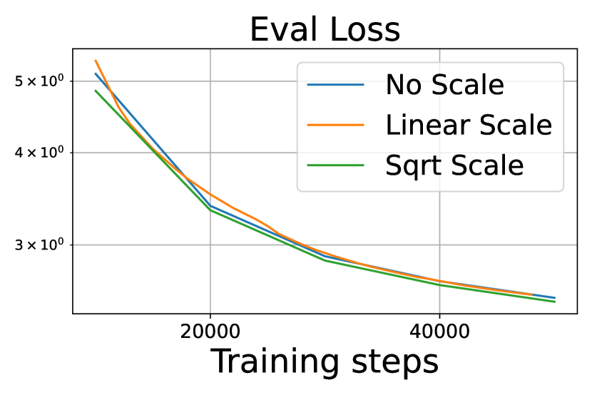
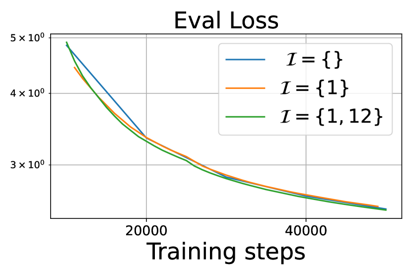
Figure 6: Ablation study on choices for RaPTr algorithm. We train BERT-base with RaPTr for 100k steps with a 6-8-10-12 schedule (see Section 4). Left to right: (a) Square-root scaling ($h_{sqrt}$) has better validation loss compared with linear scaling and no scaling at training, especially in the earlier stages. With no scale, we scale layer’s output by $1/p_{i}$ during inference (following [Huang et al., 2016]). (b) Different candidates for the fixed set $\mathcal{I}$ are compared for RaPTr. We find that training with first and last layers fixed helps faster training.

While working on subnetworks, it is important to appropriately rescale the network. In particular, bypassing layer(s) in RaPTr can shift the input distribution for layers compared to the full model. To mitigate this shift, we scale the output of the layers to maintain the norms of the input to each layer throughout training. The idea of scaling layer outputs has also been explored in prior work [Huang et al., 2016, Fan et al., 2019].We use a different square-root scaling mechanism that is motivated by analysis on a randomly initialized Transformer architecture. We show that at initialization, the norm of the intermediate outputs ${\bm{y}}^{(\ell)}$ scale as $\sqrt{\ell}$.

Theorem F.1 (Square-root scaling of input norms).

At initialization, given any input sequence ${\bm{x}}_{1:N}$ and scalars $\alpha_{1:L}$, w.h.p. the intermediate sequences of $F$ (Definition 2.1) satisfy

$$\left\|{\bm{y}}^{(\ell)}_{i}\right\|^{2}_{2}=\left\|{\bm{x}}_{i}\right\|^{2}_{2}+\Theta(\sum_{j=1}^{\ell}\alpha^{2}_{j}d),\quad\text{for all }1\leq i\leq N,1\leq\ell\leq L.$$

Inspired by this, we define the function $h_{sqrt}$ that takes in a sequence of binary values $\zeta_{1:L}\in\{0,1\}^{L}$ and returns scalars $\overline{\zeta}_{1:L}$ where $\overline{\zeta}_{i}$ is the scaling for output of layer $i$. We find a scaling that satisfies the following two conditions hold (a) $\sum_{i=1}^{j}\overline{\zeta_{i}}^{2}=j$ for all $j\leq L$ (maintaining the norm), and (b) $\overline{\zeta_{i}}=0$ if $\zeta_{i}=0$ for all $i\leq L$ (maintaining layers in random subnetwork). Formally, for each index $j$ with $\zeta_{j}=1$, it finds the index minimum $\bar{j}>j$ with $\zeta_{\bar{j}}=1$ and sets $\overline{\zeta}_{j}=\sqrt{\bar{j}-j}.$ The RaPTr algorithm with square root scaling is presented in Algorithm 1. In Figure 6 we compare square root scaling with some other scaling methods and find it to be slightly better.

F.1 Proofs

For simplicity, we present the results for transformers with single head in the self-attention layer. Furthermore, for simplicity, we use $\sigma_{relu}$ activation in the MLPs.

Algorithm 3 Transformer Layer

0:  2 layer normalization layers $f^{LN}_{attn}$, $f^{LN}_{mlp}$ (F.2), an MLP layer $f^{mlp}$ (F.4), and a softmax self-attention layer $f^{attn}$ (F.3), input sequence $\{{\bm{x}}_{n}\in\mathbb{R}^{d}\}_{n=1}^{N}$.

1:  Attention Layer normalization: returns $\{{\bm{y}}^{attnln}_{n}\}_{n=1}^{N}$ with ${\bm{y}}^{attnln}_{n}=f^{LN}_{attn}({\bm{x}}_{n})$ for all $n\leq N$.

2:  Softmax self-attention: returns $\{{\bm{y}}^{attn}_{n}\}_{n=1}^{N}=f^{attn}(\{{\bm{y}}^{attnln}_{n}\}_{n=1}^{N})$.

3:  Residual connection: returns $\{{\bm{y}}^{attnblock}_{n}\}_{n=1}^{N}$, with ${\bm{y}}^{attnblock}_{n}={\bm{x}}_{n}+{\bm{y}}^{attn}_{n}$ for all $n\leq N$.

4:  MLP Layer normalization: returns ${\bm{y}}^{mlpln}_{n}=f^{LN}_{mlp}({\bm{y}}^{attnblock}_{n})$ for all $n\leq N$.

5:  MLP function: returns $\{{\bm{y}}^{mlp}_{n}\}_{n=1}^{N}$ with ${\bm{y}}^{mlp}_{n}=f^{mlp}({\bm{y}}^{mlpln}_{n})$ for all $n\leq N$.

6:  Compute ${\bm{y}}_{n}={\bm{y}}^{mlp}_{n}+{\bm{y}}^{attnblock}_{n}$ for all $n\leq N$.

7:  Return $\{{\bm{y}}_{n}\}_{n=1}^{N}$

Definition F.2.

[Layer Normalization] Define a normalization function $f:\mathbb{R}^{d}\to\mathbb{R}^{d}$ that performs $f({\bm{x}})=({\bm{x}}-\mu)/\sigma$, where $\mu$ and $\sigma$ are the mean and standard deviation of ${\bm{x}}$, respectively. Then, layer normalization $f^{LN}:\mathbb{R}^{d}\to\mathbb{R}^{d}$ with parameters $\mathbf{\gamma},{\bm{b}}\in\mathbb{R}^{d}$ takes as input ${\bm{x}}\in\mathbb{R}^{d}$ and outputs ${\bm{y}}\in\mathbb{R}^{d}$, which is computed as ${\bm{z}}=f({\bm{x}}),{\bm{y}}=\mathbf{\gamma}\odot{\bm{z}}+{\bm{b}}.$

Definition F.3 (Softmax self-attention).

A self-attention layer $f^{attn}:\mathbb{R}^{N\times d}\to\mathbb{R}^{N\times d}$ with parameters $\{{\bm{W}}_{Q},{\bm{W}}_{K},{\bm{W}}_{V},{\bm{C}}^{attn}\in\mathbb{R}^{d\times d}\}$ takes a sequence $\{{\bm{x}}_{n}\}_{n\leq N}$ and outputs a sequence $\{{\bm{y}}_{n}\}_{n\leq N}$, such that

$${\bm{y}}_{n}={\bm{C}}^{attn}\sum_{\overline{n}=1}^{N}a_{n,\overline{n}}{\bm{v}}_{\overline{n}},$$

$$\text{with }a_{n,\overline{n}}=\mathrm{softmax}({\bm{K}}{\bm{q}}_{n})_{\overline{n}},\quad{\bm{q}}_{n}={\bm{W}}_{Q}{\bm{x}}_{n},\quad{\bm{k}}_{n}={\bm{W}}_{K}{\bm{x}}_{n},\quad{\bm{v}}_{n}={\bm{W}}_{V}{\bm{x}}_{n},$$

for all $n\leq N$, and ${\bm{K}}\in\mathbb{R}^{N\times N}$ defined with rows $\{{\bm{k}}_{n}\}_{n=1}^{N}.$

Definition F.4 (MLP).

An MLP layer $f^{mlp}:\mathbb{R}^{d}\to\mathbb{R}^{d}$ with parameters $\{{\bm{W}}\in\mathbb{R}^{m\times d},{\bm{C}}^{mlp}\in\mathbb{R}^{m\times d}\}$ and activation $\sigma_{relu}$, takes an input ${\bm{x}}\in\mathbb{R}^{d}$ and outputs ${\bm{y}}\in\mathbb{R}^{d}$, such that

$${\bm{y}}={\bm{C}}^{mlp}\sigma_{relu}({\bm{W}}{\bm{x}}).$$

Definition F.5 (Transformer layer).

A pre-layernorm transformer layer with three sub-layers; 2 layer normalization layers $f^{LN}_{attn}$, $f^{LN}_{mlp}$ (F.2), an MLP layer $f^{mlp}$ (F.4), and a softmax self-attention layer $f^{attn}$ (F.3); takes a sequence $\{{\bm{x}}_{n\leq N}$ and outputs a sequence $\{{\bm{y}}_{n}\}_{n\leq N}$ in four steps.

1. First computes $\{{\bm{y}}^{attnln}_{n}\}_{n=1}^{N}$ using a layer normalization, i.e. ${\bm{y}}^{attnln}_{n}=f^{LN}_{attn}({\bm{x}}_{n})$ for all $n\leq N$.

2. Then it runs softmax self-attention to get $\{{\bm{y}}^{attn}_{n}\}_{n=1}^{N}=f^{attn}(\{{\bm{y}}^{attnln}_{n}\}_{n=1}^{N})$.

3. The net output of the self-attention block is given by $\{{\bm{y}}^{attnblock}_{n}\}_{n=1}^{N}$, with ${\bm{y}}^{attnblock}_{n}={\bm{x}}_{n}+{\bm{y}}^{attn}_{n}$ for all $n\leq N$.

4. Before passing to the MLP function, it is passed through another layer normalization, i.e. ${\bm{y}}^{mlpln}_{n}=f^{LN}_{mlp}({\bm{y}}^{attnblock}_{n})$ for all $n\leq N$.

5. MLP function then returns $\{{\bm{y}}^{mlp}_{n}\}_{n=1}^{N}$ with ${\bm{y}}^{mlp}_{n}=f^{mlp}({\bm{y}}^{mlpln}_{n})$ for all $n\leq N$.

6. ${\bm{y}}_{n}={\bm{y}}^{mlp}_{n}+{\bm{y}}^{attnblock}_{n}$ for all $n\leq N$.

Definition F.6 (Initialization of the weights in the transformer layer).

The weights are initialized as follows:

$${\bm{C}}^{mlp},{\bm{C}}^{attn},{\bm{W}}_{Q},{\bm{W}}_{K},{\bm{W}}_{V}\sim\mathcal{N}(\mathbf{0},\frac{1}{\sqrt{d}}\mathbf{I}),$$

$${\bm{W}}\sim\mathcal{N}(\mathbf{0},\frac{\sqrt{2}}{\sqrt{m}}\mathbf{I}).$$

The parameters $\mathbf{\gamma},{\bm{b}}$ of the functions $f^{LN}_{attn},f^{LN}_{mlp}$ have been initialized as $\mathbf{1}$ and $\mathbf{0}$ respectively.

Lemma F.7 (Norm of the output of the MLP function, modification of lemma 7.1 in [Allen-Zhu et al., 2019]).

For a given input sequence $\{{\bm{y}}^{mlpln}_{n}\}_{n\leq N}$, if $\varepsilon\in(0,1]$, with probability at least $1-O(N)\cdot e^{-\Omega\left(m\varepsilon^{2}\right)}$ over the randomness of ${\bm{C}}^{mlp},{\bm{W}}$, we have

$$\forall i\in[N]:\quad\left\|{\bm{y}}^{mlp}_{n}\right\|/\left\|{\bm{y}}^{mlpln}_{n}\right\|\in[1-\varepsilon,1+\varepsilon].$$

Lemma F.8 (Norm of the output of the layer normalization layers).

Given any input sequence $\{{\bm{x}}_{n}\}_{n=1}^{N}$, under the assumption for all $n\leq N$, ${\bm{x}}_{n}-\sum_{i=1}^{d}x_{n,i}$ isn’t identically $\mathbf{0}$, we have

$$\left\|{\bm{y}}^{attnln}_{n}\right\|=\sqrt{d}$$

for all $n\leq N$.

Similar result holds for $\{{\bm{y}}^{mlpln}_{n}\}_{n=1}^{N}.$

Lemma F.9 (Norm of the output of the MLP block).

For a given input sequence $\{{\bm{y}}^{attnblock}_{n}\}_{n\leq N}$, with probability at least $1-\mathcal{O}(1)$ over the randomness of ${\bm{C}}^{mlp},{\bm{W}}$, we have

$$\left\|{\bm{y}}_{n}\right\|^{2} =\left\|{\bm{y}}^{mlp}_{n}+{\bm{y}}^{attnblock}_{n}\right\|^{2}=\left\|{\bm{y}}^{attnblock}_{n}\right\|^{2}+d$$

$$+\mathcal{O}\left(\left\|{\bm{y}}^{attnblock}_{n}\right\|\log N+(d+\left\|{\bm{y}}^{attnblock}_{n}\right\|)\frac{\log^{3/2}N}{\sqrt{m}}\right),$$

for all $n\leq N.$

Proof.

Combining Lemmas F.8 and F.7, we have for the sequence $\{{\bm{y}}^{attnblock}_{n}\}_{n\leq N}$,

$$\left|\left\|{\bm{y}}^{mlp}_{n}\right\|/\sqrt{d}-1\right|\leq\mathcal{O}\left(\frac{\sqrt{\log N}}{\sqrt{m}}\right),$$

w.p. atleast $1-\mathcal{O}(1)$.

Furthermore, due to the randomness of ${\bm{C}}^{mlp}$, we can further show that w.p. at least $1-\mathcal{O}(1)$,

$$\left|\langle{\bm{y}}^{attnblock}_{n},{\bm{y}}^{mlp}_{n}\rangle\right|\leq\mathcal{O}(\left\|{\bm{y}}^{attnblock}_{n}\right\|\log N),$$

for all $n\leq N$. Combining the two results, we have

$$\left\|{\bm{y}}_{n}\right\|^{2} =\left\|{\bm{y}}^{mlp}_{n}+{\bm{y}}^{attnblock}_{n}\right\|^{2}=\left\|{\bm{y}}^{attnblock}_{n}\right\|^{2}+d$$

$$+\mathcal{O}\left(\left\|{\bm{y}}^{attnblock}_{n}\right\|\log N+(d+\left\|{\bm{y}}^{attnblock}_{n}\right\|)\frac{\log^{3/2}N}{\sqrt{m}}\right).$$

∎

Lemma F.10 (Norm of the output of the attention block).

For a given input sequence $\{{\bm{x}}_{n}\}_{n\leq N}$, if $\varepsilon\in(0,1]$, with probability at least $1-O(1)$ over the randomness of ${\bm{C}}^{attn},{\bm{W}}_{V}$, we have

$$\forall i\in[N]:\quad\left\|{\bm{x}}_{n}\right\|^{2}\leq\left\|{\bm{y}}^{attnblock}_{n}\right\|^{2}\leq\left\|{\bm{x}}_{n}\right\|^{2}+\left\|{\bm{x}}_{n}\right\|+d+\mathcal{O}(\frac{\sqrt{\log N}}{\sqrt{d}}(d+\left\|{\bm{x}}_{n}\right\|)).$$

Proof.

From the definitions of $\{{\bm{y}}^{attnln}_{n}\}$ and $\{{\bm{y}}^{attn}_{n}\}$, we have

$${\bm{y}}^{attn}_{n}={\bm{C}}^{attn}{\bm{W}}_{V}\sum_{j\leq N}a_{n,j}{\bm{y}}^{attnln}_{j}.$$

Thus, we can use a proof similar to the proof of Lemma F.9 to argue that with the randomness of ${\bm{C}}^{attn}$ and ${\bm{W}}_{V}$,

$$\left|\frac{\left\|{\bm{y}}^{attn}_{n}\right\|}{\left\|\sum_{j\leq N}a_{n,j}{\bm{y}}^{attnln}_{j}\right\|}-1\right|\leq\mathcal{O}\left(\frac{\sqrt{\log N}}{\sqrt{d}}\right),$$

for all $n\leq N$ w.p. atleast $1-\mathcal{O}(1).$

Furthermore, due to the randomness of ${\bm{C}}^{attn}$, we can further show that w.p. atleast $1-\mathcal{O}(1)$,

$$\left|\langle{\bm{y}}^{attn}_{n},{\bm{x}}_{n}\rangle\right|\leq\mathcal{O}(\left\|{\bm{x}}_{n}\right\|\log N),$$

for all $n\leq N$.

Using Cauchy-Schwarz inequality, we must have

$$\left\|\sum_{j\leq N}a_{n,j}{\bm{y}}^{attnln}_{j}\right\|\leq\max_{j\leq N}\left\|{\bm{y}}^{attnln}_{j}\right\|=\sqrt{d}.$$

Thus, combining the results, we have

$$\left\|{\bm{y}}^{attnblock}_{n}\right\|^{2} =\left\|{\bm{y}}^{attn}_{n}+{\bm{x}}_{n}\right\|^{2}\leq\left\|{\bm{x}}_{n}\right\|^{2}+d$$

$$+\mathcal{O}\left(\left\|{\bm{x}}_{n}\right\|\log N+(d+\left\|{\bm{x}}_{n}\right\|)\frac{\log^{3/2}N}{\sqrt{d}}\right).$$

∎

Lemma F.11 (Norm of the output of the transformer layer).

For a given input sequence $\{{\bm{x}}_{n}\}_{n\leq N}$, if $\varepsilon\in(0,1]$, with probability at least $1-\mathcal{O}(1)$ over the randomness of ${\bm{C}}^{attn},{\bm{W}}_{V},{\bm{C}}^{mlp}$, we have

$$\forall i\in[N]:\quad\left\|{\bm{x}}_{n}\right\|^{2}+d+\mathcal{O}(err)\leq\left\|{\bm{y}}_{n}\right\|^{2}\leq\left\|{\bm{x}}_{n}\right\|^{2}+2d+\mathcal{O}(err),$$

where $err=\mathcal{O}\left(\left\|{\bm{x}}_{n}\right\|\log N+(d+\left\|{\bm{x}}_{n}\right\|)\frac{\log^{3/2}N}{\sqrt{m}}\right)$.

See F.1

Proof.

This follows from the fact that the transformer architecture is a stack of struturally identical $L$ transformer layers, and each transformer layer’s output norm increases by $\Theta(d)$ compared to its input norm, as given by Lemma F.11. ∎

References

- Abbe et al. [2022] Emmanuel Abbe, Enric Boix Adsera, and Theodor Misiakiewicz. The merged-staircase property: a necessary and nearly sufficient condition for sgd learning of sparse functions on two-layer neural networks. In Conference on Learning Theory, pages 4782–4887. PMLR, 2022.
- Abbe et al. [2023] Emmanuel Abbe, Enric Boix Adsera, and Theodor Misiakiewicz. Sgd learning on neural networks: leap complexity and saddle-to-saddle dynamics. In The Thirty Sixth Annual Conference on Learning Theory, pages 2552–2623. PMLR, 2023.
- Allen-Zhu et al. [2019] Zeyuan Allen-Zhu, Yuanzhi Li, and Zhao Song. A convergence theory for deep learning via over-parameterization. In International conference on machine learning, pages 242–252. PMLR, 2019.
- Ba et al. [2016] Jimmy Lei Ba, Jamie Ryan Kiros, and Geoffrey E Hinton. Layer normalization. arXiv preprint arXiv:1607.06450, 2016.
- Bachlechner et al. [2021] Thomas Bachlechner, Bodhisattwa Prasad Majumder, Henry Mao, Gary Cottrell, and Julian McAuley. Rezero is all you need: Fast convergence at large depth. In Uncertainty in Artificial Intelligence, pages 1352–1361. PMLR, 2021.
- Berant et al. [2013] Jonathan Berant, Andrew Chou, Roy Frostig, and Percy Liang. Semantic parsing on freebase from question-answer pairs. In Proceedings of the 2013 conference on empirical methods in natural language processing, pages 1533–1544, 2013.
- Brown et al. [2020] Tom Brown, Benjamin Mann, Nick Ryder, Melanie Subbiah, Jared D Kaplan, Prafulla Dhariwal, Arvind Neelakantan, Pranav Shyam, Girish Sastry, Amanda Askell, et al. Language models are few-shot learners. Advances in neural information processing systems, 33:1877–1901, 2020.
- Cao et al. [2019] Yuan Cao, Zhiying Fang, Yue Wu, Ding-Xuan Zhou, and Quanquan Gu. Towards understanding the spectral bias of deep learning. arXiv preprint arXiv:1912.01198, 2019.
- Chang et al. [2023] Shuning Chang, Pichao Wang, Hao Luo, Fan Wang, and Mike Zheng Shou. Revisiting vision transformer from the view of path ensemble. arXiv preprint arXiv:2308.06548, 2023.
- Chen et al. [2023] Xiangning Chen, Chen Liang, Da Huang, Esteban Real, Kaiyuan Wang, Yao Liu, Hieu Pham, Xuanyi Dong, Thang Luong, Cho-Jui Hsieh, et al. Symbolic discovery of optimization algorithms. arXiv preprint arXiv:2302.06675, 2023.
- Choi et al. [2018] Eunsol Choi, He He, Mohit Iyyer, Mark Yatskar, Wen-tau Yih, Yejin Choi, Percy Liang, and Luke Zettlemoyer. Quac: Question answering in context. arXiv preprint arXiv:1808.07036, 2018.
- Chowdhery et al. [2022] Aakanksha Chowdhery, Sharan Narang, Jacob Devlin, Maarten Bosma, Gaurav Mishra, Adam Roberts, Paul Barham, Hyung Won Chung, Charles Sutton, Sebastian Gehrmann, et al. Palm: Scaling language modeling with pathways. arXiv preprint arXiv:2204.02311, 2022.
- Clark et al. [2020] Jonathan H Clark, Eunsol Choi, Michael Collins, Dan Garrette, Tom Kwiatkowski, Vitaly Nikolaev, and Jennimaria Palomaki. Tydi qa: A benchmark for information-seeking question answering in ty pologically di verse languages. Transactions of the Association for Computational Linguistics, 8:454–470, 2020.
- Del Corro et al. [2023] Luciano Del Corro, Allie Del Giorno, Sahaj Agarwal, Bin Yu, Ahmed Awadallah, and Subhabrata Mukherjee. Skipdecode: Autoregressive skip decoding with batching and caching for efficient llm inference. arXiv preprint arXiv:2307.02628, 2023.
- Devlin et al. [2018] Jacob Devlin, Ming-Wei Chang, Kenton Lee, and Kristina Toutanova. Bert: Pre-training of deep bidirectional transformers for language understanding. arXiv preprint arXiv:1810.04805, 2018.
- Dong et al. [2021] Yihe Dong, Jean-Baptiste Cordonnier, and Andreas Loukas. Attention is not all you need: Pure attention loses rank doubly exponentially with depth. In International Conference on Machine Learning, pages 2793–2803. PMLR, 2021.
- Dosovitskiy et al. [2020] Alexey Dosovitskiy, Lucas Beyer, Alexander Kolesnikov, Dirk Weissenborn, Xiaohua Zhai, Thomas Unterthiner, Mostafa Dehghani, Matthias Minderer, Georg Heigold, Sylvain Gelly, et al. An image is worth 16x16 words: Transformers for image recognition at scale. arXiv preprint arXiv:2010.11929, 2020.
- Dua et al. [2019] Dheeru Dua, Yizhong Wang, Pradeep Dasigi, Gabriel Stanovsky, Sameer Singh, and Matt Gardner. Drop: A reading comprehension benchmark requiring discrete reasoning over paragraphs. arXiv preprint arXiv:1903.00161, 2019.
- Dun et al. [2022] Chen Dun, Cameron R Wolfe, Christopher M Jermaine, and Anastasios Kyrillidis. Resist: Layer-wise decomposition of resnets for distributed training. In Uncertainty in Artificial Intelligence, pages 610–620. PMLR, 2022.
- Fan et al. [2019] Angela Fan, Edouard Grave, and Armand Joulin. Reducing transformer depth on demand with structured dropout. arXiv preprint arXiv:1909.11556, 2019.
- [21] Wikimedia Foundation. Wikimedia downloads. URL https://dumps.wikimedia.org.
- Gesmundo and Maile [2023] Andrea Gesmundo and Kaitlin Maile. Composable function-preserving expansions for transformer architectures. arXiv preprint arXiv:2308.06103, 2023.
- Geva et al. [2021] Mor Geva, Roei Schuster, Jonathan Berant, and Omer Levy. Transformer feed-forward layers are key-value memories. In Proceedings of the 2021 Conference on Empirical Methods in Natural Language Processing, pages 5484–5495, Online and Punta Cana, Dominican Republic, November 2021. Association for Computational Linguistics. doi: 10.18653/v1/2021.emnlp-main.446. URL https://aclanthology.org/2021.emnlp-main.446.
- Gong et al. [2019] Linyuan Gong, Di He, Zhuohan Li, Tao Qin, Liwei Wang, and Tieyan Liu. Efficient training of bert by progressively stacking. In International conference on machine learning, pages 2337–2346. PMLR, 2019.
- Gu et al. [2020] Xiaotao Gu, Liyuan Liu, Hongkun Yu, Jing Li, Chen Chen, and Jiawei Han. On the transformer growth for progressive bert training. arXiv preprint arXiv:2010.12562, 2020.
- Gupta et al. [2018] Vineet Gupta, Tomer Koren, and Yoram Singer. Shampoo: Preconditioned stochastic tensor optimization. In International Conference on Machine Learning, pages 1842–1850. PMLR, 2018.
- He et al. [2016] Kaiming He, Xiangyu Zhang, Shaoqing Ren, and Jian Sun. Deep residual learning for image recognition. In Proceedings of the IEEE conference on computer vision and pattern recognition, pages 770–778, 2016.
- Hou et al. [2020] Lu Hou, Zhiqi Huang, Lifeng Shang, Xin Jiang, Xiao Chen, and Qun Liu. Dynabert: Dynamic bert with adaptive width and depth. Advances in Neural Information Processing Systems, 33:9782–9793, 2020.
- Houlsby et al. [2019] Neil Houlsby, Andrei Giurgiu, Stanislaw Jastrzebski, Bruna Morrone, Quentin De Laroussilhe, Andrea Gesmundo, Mona Attariyan, and Sylvain Gelly. Parameter-efficient transfer learning for nlp. In International Conference on Machine Learning, pages 2790–2799. PMLR, 2019.
- Hu et al. [2022] Edward J Hu, yelong shen, Phillip Wallis, Zeyuan Allen-Zhu, Yuanzhi Li, Shean Wang, Lu Wang, and Weizhu Chen. LoRA: Low-rank adaptation of large language models. In International Conference on Learning Representations, 2022. URL https://openreview.net/forum?id=nZeVKeeFYf9.
- Huang et al. [2016] Gao Huang, Yu Sun, Zhuang Liu, Daniel Sedra, and Kilian Q Weinberger. Deep networks with stochastic depth. In Computer Vision–ECCV 2016: 14th European Conference, Amsterdam, The Netherlands, October 11–14, 2016, Proceedings, Part IV 14, pages 646–661. Springer, 2016.
- Ioffe and Szegedy [2015] Sergey Ioffe and Christian Szegedy. Batch normalization: Accelerating deep network training by reducing internal covariate shift. In Francis Bach and David Blei, editors, Proceedings of the 32nd International Conference on Machine Learning, volume 37 of Proceedings of Machine Learning Research, pages 448–456, Lille, France, 07–09 Jul 2015. PMLR. URL https://proceedings.mlr.press/v37/ioffe15.html.
- J. Reddi et al. [2023] Sashank J. Reddi, Sobhan Miryoosefi, Stefani Karp, Shankar Krishnan, Satyen Kale, Seungyeon Kim, and Sanjiv Kumar. Efficient training of language models using few-shot learning. In Andreas Krause, Emma Brunskill, Kyunghyun Cho, Barbara Engelhardt, Sivan Sabato, and Jonathan Scarlett, editors, Proceedings of the 40th International Conference on Machine Learning, volume 202 of Proceedings of Machine Learning Research, pages 14553–14568. PMLR, 23–29 Jul 2023. URL https://proceedings.mlr.press/v202/j-reddi23a.html.
- Jathushan et al. [2019] Rajasegaran Jathushan, Hayat Munawar, H Salman, Khan Fahad Shahbaz, and Shao Ling. Random path selection for incremental learning. arXiv preprint, 2019.
- Joshi et al. [2017] Mandar Joshi, Eunsol Choi, Daniel S Weld, and Luke Zettlemoyer. Triviaqa: A large scale distantly supervised challenge dataset for reading comprehension. arXiv preprint arXiv:1705.03551, 2017.
- Kaddour et al. [2023] Jean Kaddour, Oscar Key, Piotr Nawrot, Pasquale Minervini, and Matt J Kusner. No train no gain: Revisiting efficient training algorithms for transformer-based language models. arXiv preprint arXiv:2307.06440, 2023.
- Kalimeris et al. [2019] Dimitris Kalimeris, Gal Kaplun, Preetum Nakkiran, Benjamin Edelman, Tristan Yang, Boaz Barak, and Haofeng Zhang. Sgd on neural networks learns functions of increasing complexity. Advances in neural information processing systems, 32, 2019.
- Kwiatkowski et al. [2019] Tom Kwiatkowski, Jennimaria Palomaki, Olivia Redfield, Michael Collins, Ankur Parikh, Chris Alberti, Danielle Epstein, Illia Polosukhin, Jacob Devlin, Kenton Lee, Kristina Toutanova, Llion Jones, Matthew Kelcey, Ming-Wei Chang, Andrew M. Dai, Jakob Uszkoreit, Quoc Le, and Slav Petrov. Natural questions: A benchmark for question answering research. Transactions of the Association for Computational Linguistics, 7:452–466, 2019. doi: 10.1162/tacl˙a˙00276. URL https://aclanthology.org/Q19-1026.
- Lei et al. [2023] Tao Lei, Junwen Bai, Siddhartha Brahma, Joshua Ainslie, Kenton Lee, Yanqi Zhou, Nan Du, Vincent Y Zhao, Yuexin Wu, Bo Li, et al. Conditional adapters: Parameter-efficient transfer learning with fast inference. arXiv preprint arXiv:2304.04947, 2023.
- Liu et al. [2022] Haokun Liu, Derek Tam, Mohammed Muqeeth, Jay Mohta, Tenghao Huang, Mohit Bansal, and Colin A Raffel. Few-shot parameter-efficient fine-tuning is better and cheaper than in-context learning. Advances in Neural Information Processing Systems, 35:1950–1965, 2022.
- Liu et al. [2023a] Hong Liu, Zhiyuan Li, David Hall, Percy Liang, and Tengyu Ma. Sophia: A scalable stochastic second-order optimizer for language model pre-training. arXiv preprint arXiv:2305.14342, 2023a.
- Liu et al. [2023b] Hong Liu, Sang Michael Xie, Zhiyuan Li, and Tengyu Ma. Same pre-training loss, better downstream: Implicit bias matters for language models. In International Conference on Machine Learning, pages 22188–22214. PMLR, 2023b.
- Liu et al. [2023c] Zhuang Liu, Zhiqiu Xu, Joseph Jin, Zhiqiang Shen, and Trevor Darrell. Dropout reduces underfitting. arXiv preprint arXiv:2303.01500, 2023c.
- Loshchilov and Hutter [2019] Ilya Loshchilov and Frank Hutter. Decoupled weight decay regularization. In International Conference on Learning Representations, 2019. URL https://openreview.net/forum?id=Bkg6RiCqY7.
- Mostafazadeh et al. [2017] Nasrin Mostafazadeh, Michael Roth, Annie Louis, Nathanael Chambers, and James Allen. Lsdsem 2017 shared task: The story cloze test. In Proceedings of the 2nd Workshop on Linking Models of Lexical, Sentential and Discourse-level Semantics, pages 46–51, 2017.
- O’Donnell [2014] Ryan O’Donnell. Analysis of boolean functions. Cambridge University Press, 2014.
- Paperno et al. [2016] Denis Paperno, Germán Kruszewski, Angeliki Lazaridou, Quan Ngoc Pham, Raffaella Bernardi, Sandro Pezzelle, Marco Baroni, Gemma Boleda, and Raquel Fernández. The lambada dataset: Word prediction requiring a broad discourse context. arXiv preprint arXiv:1606.06031, 2016.
- Pfeiffer et al. [2021] Jonas Pfeiffer, Aishwarya Kamath, Andreas Rücklé, Kyunghyun Cho, and Iryna Gurevych. AdapterFusion: Non-destructive task composition for transfer learning. In Proceedings of the 16th Conference of the European Chapter of the Association for Computational Linguistics: Main Volume, pages 487–503, Online, April 2021. Association for Computational Linguistics. doi: 10.18653/v1/2021.eacl-main.39. URL https://aclanthology.org/2021.eacl-main.39.
- Pham et al. [2019] Ngoc-Quan Pham, Thai-Son Nguyen, Jan Niehues, Markus Müller, Sebastian Stüker, and Alexander Waibel. Very deep self-attention networks for end-to-end speech recognition. arXiv preprint arXiv:1904.13377, 2019.
- Raffel et al. [2020] Colin Raffel, Noam Shazeer, Adam Roberts, Katherine Lee, Sharan Narang, Michael Matena, Yanqi Zhou, Wei Li, and Peter J. Liu. Exploring the limits of transfer learning with a unified text-to-text transformer. Journal of Machine Learning Research, 21(140):1–67, 2020. URL http://jmlr.org/papers/v21/20-074.html.
- Rahaman et al. [2019] Nasim Rahaman, Aristide Baratin, Devansh Arpit, Felix Draxler, Min Lin, Fred Hamprecht, Yoshua Bengio, and Aaron Courville. On the spectral bias of neural networks. In International Conference on Machine Learning, pages 5301–5310. PMLR, 2019.
- Rajpurkar et al. [2018] Pranav Rajpurkar, Robin Jia, and Percy Liang. Know what you don’t know: Unanswerable questions for squad. arXiv preprint arXiv:1806.03822, 2018.
- Reddy et al. [2019] Siva Reddy, Danqi Chen, and Christopher D Manning. Coqa: A conversational question answering challenge. Transactions of the Association for Computational Linguistics, 7:249–266, 2019.
- Saunshi et al. [2022] Nikunj Saunshi, Jordan Ash, Surbhi Goel, Dipendra Misra, Cyril Zhang, Sanjeev Arora, Sham Kakade, and Akshay Krishnamurthy. Understanding contrastive learning requires incorporating inductive biases. In Proceedings of the 39th International Conference on Machine Learning, 2022.
- Schaeffer et al. [2023] Rylan Schaeffer, Brando Miranda, and Sanmi Koyejo. Are emergent abilities of large language models a mirage? In Thirty-seventh Conference on Neural Information Processing Systems, 2023. URL https://openreview.net/forum?id=ITw9edRDlD.
- Shazeer and Stern [2018] Noam Shazeer and Mitchell Stern. Adafactor: Adaptive learning rates with sublinear memory cost. In International Conference on Machine Learning, pages 4596–4604. PMLR, 2018.
- Shen et al. [2022] Sheng Shen, Pete Walsh, Kurt Keutzer, Jesse Dodge, Matthew Peters, and Iz Beltagy. Staged training for transformer language models. In International Conference on Machine Learning, pages 19893–19908. PMLR, 2022.
- Steiner et al. [2021] Andreas Steiner, Alexander Kolesnikov, Xiaohua Zhai, Ross Wightman, Jakob Uszkoreit, and Lucas Beyer. How to train your vit? data, augmentation, and regularization in vision transformers. arXiv preprint arXiv:2106.10270, 2021.
- Tay et al. [2022] Yi Tay, Mostafa Dehghani, Vinh Q Tran, Xavier Garcia, Jason Wei, Xuezhi Wang, Hyung Won Chung, Dara Bahri, Tal Schuster, Steven Zheng, et al. Ul2: Unifying language learning paradigms. In The Eleventh International Conference on Learning Representations, 2022.
- Tolstikhin et al. [2021] Ilya O Tolstikhin, Neil Houlsby, Alexander Kolesnikov, Lucas Beyer, Xiaohua Zhai, Thomas Unterthiner, Jessica Yung, Andreas Steiner, Daniel Keysers, Jakob Uszkoreit, et al. Mlp-mixer: An all-mlp architecture for vision. Advances in neural information processing systems, 34:24261–24272, 2021.
- Touvron et al. [2021] Hugo Touvron, Matthieu Cord, Alexandre Sablayrolles, Gabriel Synnaeve, and Hervé Jégou. Going deeper with image transformers. In Proceedings of the IEEE/CVF international conference on computer vision, pages 32–42, 2021.
- Touvron et al. [2023] Hugo Touvron, Louis Martin, Kevin Stone, Peter Albert, Amjad Almahairi, Yasmine Babaei, Nikolay Bashlykov, Soumya Batra, Prajjwal Bhargava, Shruti Bhosale, et al. Llama 2: Open foundation and fine-tuned chat models. arXiv preprint arXiv:2307.09288, 2023.
- Veit et al. [2016] Andreas Veit, Michael J Wilber, and Serge Belongie. Residual networks behave like ensembles of relatively shallow networks. Advances in neural information processing systems, 29, 2016.
- Wang et al. [2018] Alex Wang, Amanpreet Singh, Julian Michael, Felix Hill, Omer Levy, and Samuel R Bowman. Glue: A multi-task benchmark and analysis platform for natural language understanding. arXiv preprint arXiv:1804.07461, 2018.
- Wang et al. [2019] Alex Wang, Yada Pruksachatkun, Nikita Nangia, Amanpreet Singh, Julian Michael, Felix Hill, Omer Levy, and Samuel Bowman. Superglue: A stickier benchmark for general-purpose language understanding systems. Advances in neural information processing systems, 32, 2019.
- Wang et al. [2023] Peihao Wang, Rameswar Panda, Lucas Torroba Hennigen, Philip Greengard, Leonid Karlinsky, Rogerio Feris, David Daniel Cox, Zhangyang Wang, and Yoon Kim. Learning to grow pretrained models for efficient transformer training. arXiv preprint arXiv:2303.00980, 2023.
- Wei et al. [2022] Jason Wei, Yi Tay, Rishi Bommasani, Colin Raffel, Barret Zoph, Sebastian Borgeaud, Dani Yogatama, Maarten Bosma, Denny Zhou, Donald Metzler, Ed H. Chi, Tatsunori Hashimoto, Oriol Vinyals, Percy Liang, Jeff Dean, and William Fedus. Emergent abilities of large language models. Transactions on Machine Learning Research, 2022. ISSN 2835-8856. URL https://openreview.net/forum?id=yzkSU5zdwD. Survey Certification.
- Xin et al. [2020] Ji Xin, Raphael Tang, Jaejun Lee, Yaoliang Yu, and Jimmy Lin. Deebert: Dynamic early exiting for accelerating bert inference. arXiv preprint arXiv:2004.12993, 2020.
- Xu et al. [2019] Zhi-Qin John Xu, Yaoyu Zhang, Tao Luo, Yanyang Xiao, and Zheng Ma. Frequency principle: Fourier analysis sheds light on deep neural networks. arXiv preprint arXiv:1901.06523, 2019.
- Zellers et al. [2019] Rowan Zellers, Ari Holtzman, Yonatan Bisk, Ali Farhadi, and Yejin Choi. Hellaswag: Can a machine really finish your sentence? arXiv preprint arXiv:1905.07830, 2019.
- Zhang et al. [2019] Hongyi Zhang, Yann N Dauphin, and Tengyu Ma. Fixup initialization: Residual learning without normalization. arXiv preprint arXiv:1901.09321, 2019.
- Zhang and He [2020] Minjia Zhang and Yuxiong He. Accelerating training of transformer-based language models with progressive layer dropping. Advances in Neural Information Processing Systems, 33:14011–14023, 2020.
- Zhou et al. [2020] Wangchunshu Zhou, Canwen Xu, Tao Ge, Julian McAuley, Ke Xu, and Furu Wei. Bert loses patience: Fast and robust inference with early exit. Advances in Neural Information Processing Systems, 33:18330–18341, 2020.