Evaluation of the Real-time El Niño Forecasts by the Climate Network Approach between 2011 and Present

Abstract

El Niño episodes are part of the El Niño-Southern Oscillation (ENSO), which is the strongest driver of interannual climate variability, and can trigger extreme weather events and disasters in various parts of the globe. Previously we have described a network approach that allows to forecast El Niño events about 1 year ahead. Here we evaluate the real-time forecasts of this approach between 2011 and 2022. We find that the approach correctly predicted (in 2013 and 2017) the onset of both El Niño periods (2014-2016 and 2018-2019) and generated only 1 false alarm in 2019. In June 2022, the approach correctly forecasted the onset of an El Niño event in 2023. We show how to determine the $p$-value of the 12 real-time forecasts between 2011 and 2022 and find $p\cong 0.005$, this way strongly rejecting the null hypothesis that the same quality of the forecast can be obtained by random guessing. We also discuss how the algorithm can be further improved by reducing the number of false alarms in the network model forecast. When combined with other statistical methods, a more detailed forecast, including the magnitude of the event and its type, can be obtained. For 2024, the method indicates the absence of a new El Niño event.

1 Introduction

The El Niño-Southern Oscillation (ENSO) (Dijkstra, 10, Clarke, 7, Sarachik and Cane, 47, Wang et al., 52, Timmermann et al., 48, McPhaden et al., 36) can be considered as a quasi-oscillation of the Pacific ocean-atmosphere system, consisting of irregular warm (“El Niño”) and cold (“La Niña”) deviations from the long-term mean. Strong El Niño episodes can lead to extreme weather events (like extreme rainfall and droughts) in various parts of the globe (Davis, 9, Wen, 54, Kovats et al., 27, Donnelly et al., 14, Corral et al., 8, McPhaden et al., 36). To mitigate at least some of the adverse societal and economic impacts, early forecasts of El Niño events are thus highly desirable.

To forecast El Niño events, many state-of-the-art coupled climate models, as well as a variety of statistical approaches (Cane and Zebiak, 2, Penland and Sardeshmukh, 43, Tziperman et al., 51, Fedorov et al., 16, Galanti et al., 18, Kirtman, 26, Chen et al., 4, Palmer et al., 42, Luo et al., 35, Chen and Cane, 5, Chekroun et al., 6, Saha et al., 46, Chapman et al., 3, Feng et al., 17, Lu et al., 28, Rodriguez-Mendez et al., 45, Meng et al., 37, Noteboom et al., 41, Ham et al., 21, DeCastro et al., 12, Petersik et al., 44, Hassanibesheli et al., 22), have been suggested, and monthly updated overviews of the latest operational forecasts (consisting of 17 dynamical and 9 statistical methods) are available from the International Research Institute for Climate and Society (IRI, 23). While these forecasts are quite successful at shorter lead times, they have limited anticipation power at larger lead times. In particular, they generally fail to overcome the so-called “spring barrier” (see, e.g., Webster, 53, Goddard et al., 19), which shortens their typical warning time to around 6 months (Barnston et al., 1, McPhaden et al., 36) (see also the discussion in Tippett et al., 49).

In 2012, an alternative forecasting approach (Ludescher et al., 29, 30) (see also Ludescher et al., 31) has been suggested, which is based on complex-networks analysis (Tsonis et al., 50, Yamasaki et al., 55, Donges et al., 13, Gozolchiani et al., 20, Dijkstra et al., 11, Fan et al., 15, Ludescher et al., 32). The approach analyses the strength of the cooperativity represented by the mean link strength $S(t)$ in a Pacific climate network, and gives an alarm when $S$ crosses a fixed threshold, predicting a new El Niño episode to come in the following year. The optimal threshold $\Theta$ was determined in a learning period between 1950 and 1980. In the period between 1981 and 2011, this threshold $\Theta$ was used to hindcast the presence (alarm) or absence (no alarm) of a new El Niño event in the following year. After the threshold is fixed, there is no free parameter in the approach.

The procedure to split the known data (at that time between 1950 and 2011) into a learning phase and a hindcasting phase is necessary for statistical forecasting methods and aims to reduce the risk of an overfitting to spurious precursors. But the mere fact that each algorithm, when being developed, can only make “predictions" of events that have already occurred automatically introduces a certain “publication" bias, because only those algorithms that are successful in both the learning and hindcasting phase will be considered and published.

The true test for statistical forecasts are real-time forecasts. For the climate network approach, the period of real-time forecasts started in 2011. Here we evaluate the real-time forecasts of the network approach. First, in Section 2, we describe how El Niño-events are classified by the Oceanic Niño Index (ONI) and list the ONI values between 2011 and present. Next, in Section 3, we briefly describe the climate network approach. In Sections 4 and 5, we analyse its real-time forecasts between 2011 and present and determine the statistical significance of the forecast. In Section 6, we describe an improvement of the algorithm, which is based on the false alarm statistics.

2 Data

The ENSO phenomenon is quantified by the Oceanic Niño Index (ONI), which is defined as the three-month running-mean sea surface temperature (SST) anomalies in the Niño3.4 region (see Fig. 1) and is a principal measure for monitoring, assessing, and predicting ENSO.

An El Niño-episode is said to occur when the index is at least 0.5°C above the average for a period of at least 5 months. Table 1 shows the ONI between 2012 and present, as communicated by the National Oceanic and Atmospheric Administration (NOAA) (CPC, 40). The El Niño periods are in boldface. The table shows that there were no El Niño periods in 2012, 2013, 2017, 2020, 2021, and 2022. In May 2023, an El Niño started and is still ongoing at the time of writing.

Year	DJF	JFM	FMA	MAM	AMJ	MJJ	JJA	JAS	ASO	SON	OND	NDJ
2012	-0.9	-0.7	-0.6	-0.5	-0.3	0.0	0.2	0.4	0.4	0.3	0.1	-0.2
2013	-0.4	-0.4	-0.3	-0.3	-0.4	-0.4	-0.4	-0.3	-0.3	-0.2	-0.2	-0.3
2014	-0.4	-0.5	-0.3	0.0	0.2	0.2	0.0	0.1	0.2	0.5	0.6	0.7
2015	0.5	0.5	0.5	0.7	0.9	1.2	1.5	1.9	2.2	2.4	2.6	2.6
2016	2.5	2.1	1.6	0.9	0.4	-0.1	-0.4	-0.5	-0.6	-0.7	-0.7	-0.6
2017	-0.3	-0.2	0.1	0.2	0.3	0.3	0.1	-0.1	-0.4	-0.7	-0.8	-1.0
2018	-0.9	-0.9	-0.7	-0.5	-0.2	0.0	0.1	0.2	0.5	0.8	0.9	0.8
2019	0.7	0.7	0.7	0.7	0.5	0.5	0.3	0.1	0.2	0.3	0.5	0.5
2020	0.5	0.5	0.4	0.2	-0.1	-0.3	-0.4	-0.6	-0.9	-1.2	-1.3	-1.2
2021	-1.0	-0.9	-0.8	-0.7	-0.5	-0.4	-0.4	-0.5	-0.7	-0.8	-1.0	-1.0
2022	-1.0	-0.9	-1.0	-1.1	-1.0	-0.9	-0.8	-0.9	-1.0	-1.0	-0.9	-0.8
2023	-0.7	-0.4	-0.1	0.2	0.5	0.8	1.1	1.3	1.6	1.8	1.9	2.0

Table 1: Oceanic El Niño Index (ONI) 2012 - present (from CPC, 40)

3 The climate network approach

The structure of the climate network considered here is shown in Fig. 1. The network is based on a combination of the networks introduced by (Yamasaki et al., 55) and (Gozolchiani et al., 20), who studied cooperative phenomena during El Niño events. The nodes of the network consist of 14 grid points in the “El Niño basin” (red circles) (Gozolchiani et al., 20) (which roughly covers the Niño1, Niño2, Niño3, and Niño3.4 regions), and 193 grid points outside this domain (blue circles) (Yamasaki et al., 55).

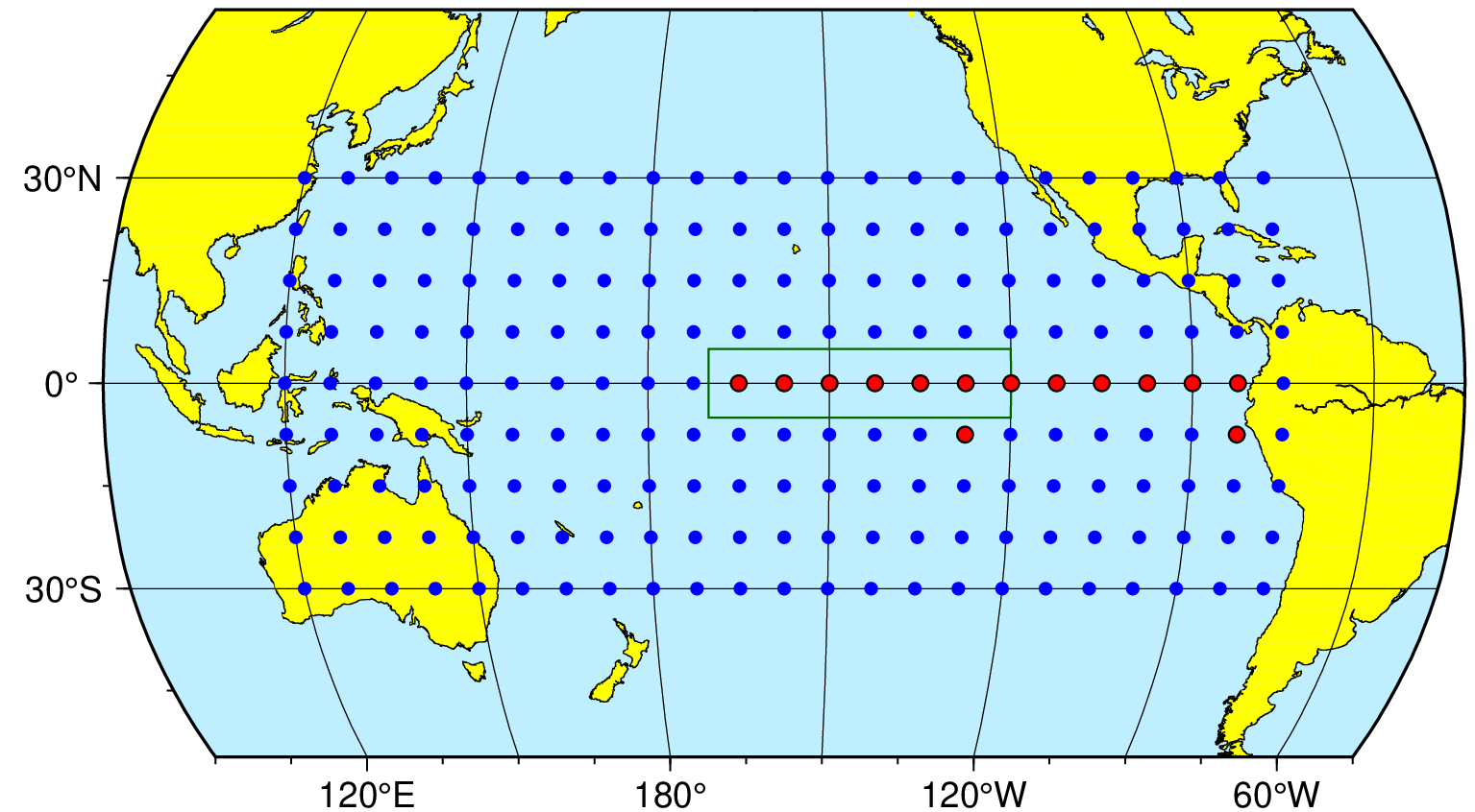
Figure 1: The structure of the climate network. Each of the 14 grid points in the “El Niño basin” (red circles) is linked to each of the 193 grid points outside this domain (blue circles). The green rectangle denotes the Niño3.4 region.

The green rectangle denotes the Niño3.4 region where the ONI is calculated. The grid points are the nodes of the climate network and are characterized by their surface air temperature (SAT) anomaly. The SAT data are obtained from the NCEP Reanalysis 1 dataset (Kalnay et al., 25, NCEP-NCAR, 39).

Each node inside the El Niño basin is linked to each node outside the basin. The link strength between two nodes (i.e., the strength of the teleconnections between them) at a given time $t$ is determined from the values of their time-lagged cross-correlation (see Appendix A) for which we consider time lags between 0 and 200 days. For each pair of nodes $i$ and $j$, we determine, for the given time $t$, the maximum, the mean, and the standard deviation around the mean of the absolute value of the cross-correlation function, and define the link strength $S_{ij}(t)$ as the difference between the maximum and the mean value, divided by the standard deviation. Accordingly, $S_{ij}(t)$ describes the link strength relative to the underlying background noise (signal-to-noise ratio). By averaging over all individual links in the network at a given instant $t$, one obtains the mean link strength $S(t)$, which is the crucial entity in the climate network approach (for details, see (Gozolchiani et al., 20, Ludescher et al., 30) and Appendix A). The variation of $S(t)$ with time $t$ can be considered as a measure of the way the cooperativity between the equatorial “El Niño basin" and the rest of the tropical and subtropical Pacific region changes with time $t$. $S(t)$ has a remarkable property: it typically decays during an El Niño event (Ludescher et al., 30) and rises in the year before an event starts. This rise of $S(t)$ can be used as a precursor for the event (Ludescher et al., 30, 31).

The optimized algorithm involves an empirical decision threshold $\Theta$. Whenever $S$ crosses $\Theta$ from below while the most recent ONI (see Data section) is below 0.5°C, the algorithm sounds an alarm and predicts the start of a new El Niño episode in the following year. Otherwise, it predicts the absence of a new El Niño event.

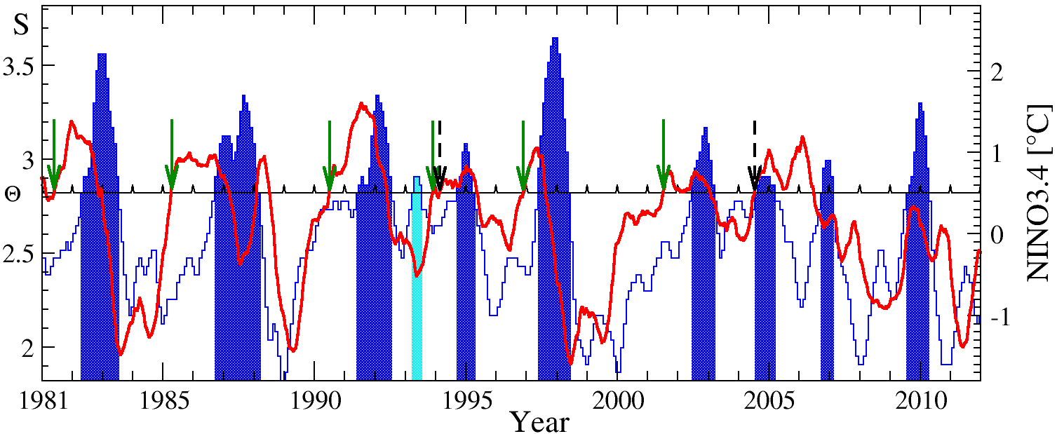
Figure 2: The forecasting scheme. We compare the average link strength $S(t)$ in the climate network (red curve) with the decision threshold $\Theta=2.82$ (horizontal line) and the ONI (right scale), between January 1981 and December 2011. When the link strength crosses the threshold from below and the last available ONI is below 0.5°C, we give an alarm and predict that a new El Niño episode will start in the following calendar year. Periods with an ONI greater or equal 0.5°C are displayed in blue. The El Niño episodes (when the ONI is greater or equal 0.5°C for at least 5 months) are displayed in dark blue. Correct predictions are marked by green arrows and false alarms by dashed arrows. Note that the early false alarms in February 1994 and July 2004 are followed by at least one ONI value equal or above 0.5°C in the same year.

In the learning phase between 1950 and 1980, all thresholds above the temporal mean of $S(t)$ were considered and the optimal ones, i.e., those ones that lead to the best predictions in the learning phase, were determined. $\Theta$-values between $2.815$ and $2.834$ lead to the best performance (Ludescher et al., 30), with a false alarm rate of 1/20.

In the hindcasting phase (1981-2011) (see Fig. 2, where $\Theta=2.82$), the performance of these thresholds was tested; thresholds between 2.815 and 2.826 gave the best results. Figure 2 shows that the alarms were correct in 75% and the non-alarms in 86% of all cases. For $\Theta$-values between $2.827$ and $2.834$, the performance was only slightly weaker.

4 Real-time forecasts between 2011 and present

Figure 3 shows the forecasts of the network approach between 2011 and 2022.

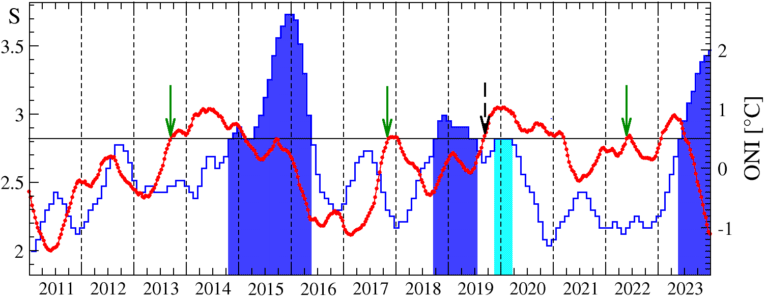
Figure 3: The real-time forecasts. Same as Fig. 2, but for the period between January 2011 and December 2023. As in Fig. 2, the false alarm (in 2019) is followed by at least one ONI value equal to or above 0.5°C in the same year. Only alarms until 2022, where the outcome is known, are marked by arrows.

In 4 years (2013, 2017, 2019, and 2022) the algorithm predicted the onset of a new El Niño event in the following calendar year. Only the alarm of 2019 was a false alarm. The present El Niño started in May 2023, so the alarm given in June 2022 was also correct.

In 8 years (2011, 2012, 2014, 2015, 2016, 2018, 2020, 2021) the approach did not give an alarm and thus correctly predicted the absence of a new El Niño in the following year. This is true also for 2014, since in 2015 no new El Niño episode, separated from the foregoing one by at least one ONI value below 0.5, started. Also these forecasts of the absence of a new El Niño event are far from being trivial as a comparison with the official forecasts by the International Research Institute for Climate and Society (IRI, 24) shows:

(i) While the climate network approach already in December 2011 indicated the absence of a new El Niño in 2012, the CPC/IRI consensus probabilistic ENSO forecast provided in August and September 2012 75 and 65 percent probability, respectively, for the presence of El Niño conditions in December 2012 (NDJ).

(ii) In spring 2017, most dynamical and statistical models falsely predicted an event in 2017. For instance, the vast majority of the ensemble members of the North American Multimodel forecasted, in April 2017, positive anomalies, while the actual SSTA turned out to be negative (Tippett et al., 49).

Indeed, according to (Tippett et al., 49), climate models tend to predict warming when initialized after observed warming conditions and cooling when initialized after observed cooling conditions, and thus failed to capture the correct direction of ENSO evolution in half of the 8 springs between 2011 and 2018.

Next, we turn to the question whether the real-time forecasts of the climate network approach are statistically significant, i.e., whether the same performance can be obtained by random guessing or not.

5 Statistical significance of the forecasts

For obtaining the statistical significance of a given configuration $K_{0}$ containing $N$ forecasts with $n_{c}$ correct alarms and $n_{f}$ false alarms, one has to determine the probability $w_{0}$ that a configuration with the same number $n_{c}$ of correct alarms and the same number $n_{f}$ of false alarms can be obtained by randomly guessing. In addition, one has to consider all configurations $K_{1},K_{2},\dots,K_{m}$ with a better or equal quality of forecast and determine the corresponding probabilities $w_{1},w_{2},\dots,w_{m}$. Then the probability $p$ that by randomly guessing the same or better forecasts can be made is given by

$$p=\sum_{i=0}^{m}w_{i},$$ (1)

$p$ is called the $p$-value. In our case, the null hypothesis is that the given forecast configuration can be obtained by randomly guessing with the climatological El Niño onset probability. When $p$ is below 0.05, the null hypothesis is rejected and the forecasts are called statistically significant at a 0.05 level; when $p$ is below 0.01, the forecasts are called highly significant. For determining the probabilities $w_{i}$, we first need to determine the occurrence probability $q$ of the onset of El Niño episodes. In the 43 years between January 1981 and 2023, 12 El Niño episodes started, so the occurrence probability is $q=12/43\cong 0.279$. First we focus on the occurrence of new El Niño episodes in the period between January 2012 and December 2023. Denoting years where a new event started by $+$ and years where no new event started by $-$, the observed configuration of years with and without new El Niño events is

$$(-,-,+,-,-,-,+,-,-,-,-,+),$$ (2)

where the most left symbol refers to 2012 and the right-most symbol to 2023 where a new El Niño episode started in May. For the period between 2012 and 2023, the network approach predicted the configuration

$$(-,-,+,-,-,-,+,-,+,-,-,+),$$ (3)

which differs from the observed configuration only in the year 2020 (+ instead -), where a new event was falsely predicted to come.

There are 9 possible configurations where one of the $-$ signs in the observed configuration (2) is changed into a $+$ sign, and all have the same quality of forecast. Accordingly, the probability of randomly guessing one of these 9 configurations is $w_{0}=9q^{4}(1-q)^{8}$.

There is only one better forecast possible: the probability $w_{1}$ of randomly guessing the observed configuration (2) is $w_{1}=q^{3}(1-q)^{9}$. Accordingly, the $p$-value of the real-time forecasts is

$$p=9q^{4}(1-q)^{8}+q^{3}(1-q)^{9}.$$ (4)

This yields, with $q=12/43$,

$$p\cong 5.1\times 10^{-3},\\ \ {\rm period\\ \ 2011-present},$$ (5)

which is well below the high-significance threshold $p=10^{-2}$.

When we consider both the hindcasting and forecasting period (January 1981 - December 2023) the $p$-value is obtained in exactly the same way, but there are more configurations to be considered. In the 43 years between 1981 and 2023, 12 new El Niño episodes started. In the 42 target years between 1982 and 2023, the network algorithm correctly forecasted 9 of these events and gave 3 false alarms. Accordingly, the hit rate $\alpha_{+}$ defined as the number of correct alarms $n_{c}$ divided by the number of events, is 9/12, while the false alarm rate, defined as the number of false alarms $n_{f}$ divided by the number of non-events, is 1/10. Thus the rate $\alpha_{-}$ of correctly predicted non-events is $(30-3)/30=9/10$. Both numbers, $\alpha_{+}$ and $\alpha_{-}$ quantify the performance of the algorithm. The probability of randomly guessing a configuration with $n_{c}$ correct events and $n_{f}$ false events is given by

$$w=\binom{12}{n_{c}}\binom{30}{n_{f}}q^{n_{c}+n_{f}}(1-q)^{42-n_{c}-n_{f}}.$$ (6)

The binomial coefficients describe the number of ways $n_{c}$ events can be chosen out of 12 events and $n_{f}$ false events out of 30 non-events; $q=12/43$ as above.

We need to determine $w$ for all configurations with a similar or better predictive power. A natural measure for the predictive power is $P={(\alpha_{+}+\alpha_{-})-1}$, which is 1 when the forecast is perfect and 0 when the forecast is purely random. Here, $P=(3/4+9/10)-1=0.65$.

Accordingly, for estimating the $p$-value of our forecast, we take into account all configurations with a higher or equal predictive power, i.e., ($n_{c}=8,n_{f}=0$), ($n_{c}=9,n_{f}=0,1,2,3$), ($n_{c}=10,n_{f}=0,1,\dots,5$), ($n_{c}=11,n_{f}=0,1,\dots,8$), and ($n_{c}=12,n_{f}=0,1,\dots,10$). For each of these combinations of $(n_{c},n_{f})$, we determine $w$ from (6) and sum up (1) the obtained probabilities. The result is

$$p\cong 3.0\times 10^{-5},\\ \ {\rm period\\ \ 1981-present}.$$ (7)

6 Further improvement of the algorithm based on the false alarm characteristics

Figures 2 and 3 show that all false alarms in the hindcasting and forecasting period (1994, 2004, and 2019) are followed by at least one ONI value equal or above 0.5°C in the same calendar year. This suggests that there may be only a low chance that an alarm is correct when the ONI does not stay below 0.5°C for the rest of the year. Accordingly, an improved algorithm based on this feature may consist of 2 steps. (i) In the first step, a (preliminary) alarm is given when $S$ crosses the threshold from below, indicating the possible appearance of an El Niño event in the following year. This alarm can occur at any time in a calendar year. (ii) When the ONI stays below 0.5°C until the end of December, this alarm is confirmed. Otherwise, the alarm is withdrawn and the absence of an El Niño onset is predicted for the following year.

When applying the improved algorithm to the period between 2011 and 2022, all forecasts turn out to be correct, resulting in a $p$-value $p=q^{3}(1-q)^{9}\cong 1.1\times 10^{-3}$. For the hindcasting plus forecasting period (1981-present), all 9 El Niño onset alarms are correct and there are 3 missed El Niño events resulting in $p\cong 1.4\times 10^{-6}$.

Figure 3 shows that in January 2023, the mean link strength $S(t)$ crossed the threshold $\Theta$, giving a preliminary alarm. However, since an El Niño started afterwards, the ONI did not stay below 0.5°C until December 2023. Therefore, this preliminary alarm is withdrawn, indicating the absence of an El Niño onset in 2024. Since there were 3 missed El Niño events between 1981 and 2023 and 30 correct predictions for the absence of a new El Niño, the probability for the absence of an El Niño onset in 2024 is 30/33 $\approx 90.9\%$.

7 Conclusions

In summary, we have evaluated the quality of the real-time El Niño forecasts made by the climate network approach. We have shown how to determine the statistical significance of the forecasts and found that its $p$-value is well below the generally accepted high-significance level $p=0.01$, this way clearly rejecting the null hypothesis that the same performance might be obtained by simple random guessing. We are not aware of any other method that allows, within a period of 12 years, a similar quality of real-time forecasts with a lead time of about 1 y.

The climate network approach suggests that the emergence of cooperativity between the El Niño basin and the rest of the Pacific is an important prerequisite for the development of an El Niño event in the following year. We can speculate that the westerly wind bursts are more effective in initiating a large scale El Niño event when the Pacific is in a cooperative state, and this would explain the success of the complex network approach. But, a detailed analysis remains for future work.

The high prediction skill of the forecast and its long lead time should allow early mitigation methods. One of the advantages of the network approach is that it does not contain a freely choosable fit parameter. The underlying climate network was introduced in a different context and independently of any El Niño forecasting well before it was used to forecast El Niño events. Also the parameters used in the calculation of the link strengths had been fixed before (Yamasaki et al., 55). The only new parameter in the algorithm, the threshold $\Theta$, was fixed in the learning phase (Ludescher et al., 30). The reanalysis (NCEP) temperature data can be easily obtained from (NCEP-NCAR, 39). Since also the calculation of the link strengths is straightforward and not computationally demanding, the network approach can be easily used to obtain real-time El Niño forecasts, which is an additional advantage besides the long lead time.

The climate network-based approach discussed here forecasts the onset or absence of an El Niño event in the following calendar year with high accuracy. The approach can be combined (Ludescher et al., 33) with additional statistical forecasting methods for the magnitude (Meng et al., 38) and type (Ludescher et al., 34) of an event. This way, the events’s risk potential can be estimated much in advance, and thus, more time becomes available to plan and implement adapted mitigation measures.

So far, the climate network approach has been applied only to forecasting the onset of an El Niño episode. It is an open question, how to extend it to early forecast also La Niña episodes. The majority of El Niño episodes, in particular the strong ones, are followed by a La Niña in the consecutive year, so here, the forecast is more straightforward. But often, 2-year or even 3-year La Niña episodes, like the one between 2020 and 2023, occur, and the challenge is to predict both the onset and the length of a La Niña episode. We think that a combination of the climate network approach with deterministic approaches that can take advantage of ENSO’s quasi-oscillatory nature may be instrumental in developing an early forecasting approach for La Niña episodes.

Appendix A Calculation of the mean link strength in the network approach

This Appendix follows closely (Ludescher et al., 31). For the prediction of the onset of El Niño events or non-events we use the cooperative behavior of the atmospheric temperatures in the Pacific as a precursor. To obtain a measure for the cooperativity, we consider the daily surface atmospheric temperature anomalies (SATA) between January 1950 and December 2023 at the grid points (”nodes”) of a Pacific network, see Fig. 1.

We analyse the time evolution of the teleconnections (“links”) between the temperatures at nodes $i$ inside the “El Niño basin” and nodes $j$ outside the basin. The strengths of these links are represented by the strengths of the cross correlations between the temperature records at these sites (Yamasaki et al., 55).

The prediction algorithm (Ludescher et al., 30, 31) is as follows:

(1) At each node $k$ of the network shown in Fig. 1, the daily atmospheric temperature anomalies $T_{k}(t)$ (actual temperature value minus climatological average for each calendar day, see below) at the surface area level is determined. For the calculation of the climatological average, the leap days have been removed. The data have been obtained from the National Centers for Environmental Prediction/National Center for Atmospheric Research Reanalysis I project (Kalnay et al., 25, NCEP-NCAR, 39).

(2) For obtaining the time evolution of the strengths of the links between the nodes $i$ inside the El Niño basin and the nodes $j$ outside we compute, for each 10th day $t$ in the considered time span between January 1950 and December 2023, the time-delayed cross-correlation function defined as

$$C_{i,j}^{(t)}(-\tau)=\frac{\langle T_{i}(t)T_{j}(t-\tau)\rangle-\langle T_{i}(t)\rangle\langle T_{j}(t-\tau)\rangle}{\sqrt{\langle(T_{i}(t)-\langle T_{i}(t)\rangle)^{2}\rangle}\cdot\sqrt{\langle(T_{j}(t-\tau)-\langle T_{j}(t-\tau)\rangle)^{2}\rangle}}$$

and

$$C_{i,j}^{(t)}(\tau)=\frac{\langle T_{i}(t-\tau)T_{j}(t)\rangle-\langle T_{i}(t-\tau)\rangle\langle T_{j}(t)\rangle}{\sqrt{\langle(T_{i}(t-\tau)-\langle T_{i}(t-\tau)\rangle)^{2}\rangle}\cdot\sqrt{\langle(T_{j}(t)-\langle T_{j}(t)\rangle)^{2}\rangle}}$$

where the brackets denote an average over the past 365 d, according to

$$\langle f(t)\rangle=\frac{1}{365}\sum_{m=0}^{364}f(t-m).$$

We consider time lags $\tau$ between 0 and 200 d, where a reliable estimate of the background noise level can be guaranteed.

(3) We determine, for each point in time $t$, the maximum, the mean, and the standard deviation around the mean of the absolute value of the cross-correlation function $|C_{ij}^{(t)}(\tau)|$ and define the link strength $S_{ij}(t)$ as the difference between the maximum and the mean value, divided by the standard deviation. Accordingly, $S_{ij}$ describes the link strength at day t relative to the underlying background noise (signal-to-noise ratio) and thus quantifies the dynamical teleconnections between nodes i and j.

(4) To obtain the desired mean strength $S(t)$ of the dynamical teleconnections in the climate network, we simply average over all individual link strengths.

(5) Finally, we compare $S(t)$ with a decision threshold $\Theta$. When the link strength $S(t)$ crosses the threshold from below and the last available ONI at that time $t$ is below 0.5°C, we give an alarm and predict that an El Niño episode will start in the following calendar year.

We like to add that for the calculation of the climatological average in the learning phase, all data within this time window have been taken into account, while in the prediction phase, only data from the past up to the prediction date have been considered.

Declarations

• Funding JL was supported by the ”Brazil East Africa Peru India Climate Capacities (B-EPICC)“ project, which is part of the International Climate Initiative (IKI) of the German Federal Ministry for Economic Affairs and Climate Action (BMWK) and implemented by the Federal Foreign Office (AA).

• Competing interests The authors declare no competing interests.

• Data availability The data sources for this study are publicly available and referenced in the text.

References

- Barnston et al., [2012] Barnston, AG, Tippett MK, L’Heureux ML, Li S, DeWitt DG (2012) Skill of real-time seasonal ENSO model predictions during 2002-11: Is our capability increasing? Bulletin of the American Meteorological Society 93(5), 631-651.
- Cane and Zebiak, [1986] Cane MA, Zebiak SE, Dolan SC (1986) Experimental forecasts of El Niño. Nature 321:827-832.
- Chapman et al., [2015] Chapman D, Cane MA, Henderson N, Lee DE, Chen C (2015) A Vector Autoregressive ENSO Prediction Model. J Clim 28:8511-8520.
- Chen et al., [2004] Chen D, Cane MA, Kaplan A, Zebiak SE, Huang D (2004) Predictability of El Niño over the past 148 years. Nature 428:733-736.
- Chen and Cane, [2008] Chen D, Cane MA (2008) El Niño prediction and predictability. J Comput Phys 227:3625-3640.
- Chekroun et al., [2011] Chekroun MD, Kondrashov D, Ghil M (2011) Predicting stochastic systems by noise sampling, and application to the El Niño-Southern Oscillation. Proc Nat Acad Sci USA 108(29):11766-11771.
- Clarke, [2008] Clarke AJ (2008) An Introduction to the Dynamics of El Niño and the Southern Oscillation (Elsevier Academic Press, London).
- Corral et al., [2010] Corral A, Ossó A, Llebot JE (2010) Scaling of tropical-cyclone dissipation. Nature Phys 6:693-696.
- Davis, [2001] Davis M (2001) Late Victorian Holocaust: El Niño Famines and the Making of the Third World (Verso, London & New York).
- Dijkstra, [2005] Dijkstra HA (2005) Nonlinear Physical Oceanography: A Dynamical Systems Approach to the Large-Scale Ocean Circulation and El Niño (Springer, New York).
- Dijkstra et al., [2019] Dijkstra HA, Hernández-García E, Masoller C, Barreiro M (2019) Networks in Climate (Cambridge Univ Press, Cambridge, UK).
- DeCastro et al., [2020] De Castro Santos MA, Vega-Oliveros DA, Zhao L, Berton L (2020) Classifying El Niño-Southern Oscillation combining network science and machine learning. IEEE Access 8, 55711-55723.
- Donges et al., [2009] Donges JF, Zou Y, Marwan N, Kurths J (2009) The backbone of the climate network. EPL (Europhysics Letters) 87(4):48007.
- Donnelly et al., [2007] Donnelly JP, Woodruff JD (2007) Intense hurricane activity over the past 5,000 years controlled by El Niño and the West African monsoon. Nature 447:465-468.
- Fan et al., [2021] Fan J, Meng J, Ludescher J, Chen X, Ashkenazy Y, Kurths J, Havlin S, Schellnhuber HJ (2021) Statistical physics approaches to the complex Earth system. Physics Reports 896:1-84.
- Fedorov et al., [2003] Fedorov AV, Harper SL, Philander SG, Winter B, Wittenberg A (2003) How Predictable is El Niño? Bull Amer Meteor Soc 84:911-919.
- Feng et al., [2016] Feng QY et al. (2016) ClimateLearn : A machine-learning approach for climate prediction using network measures. Geosci. Model Dev. 10.5194/gmd-2015-273.
- Galanti et al., [2003] Galanti E, Tziperman E, Rosati A, Sirkes Z (2003) A Study of ENSO Prediction Using a Hybrid Coupled Model and the Adjoint Method for Data Assimilation. Mon Weather Rev 131:2748-2764.
- Goddard et al., [2001] Goddard L et al. (2001) Current approaches to seasonal to interannual climate predictions. Int J Clim 21:1111-1152.
- Gozolchiani et al., [2011] Gozolchiani A, Yamasaki K, Havlin S (2011) Emergence of El Niño as an autonomous component in the climate network. Phys Rev Lett 107(14):148501.
- Ham et al., [2019] Ham YG, Kim JH,Luo, JJ (2019) Deep learning for multi-year ENSO forecasts. Nature, 573, 568-572.
- Hassanibesheli et al., [2022] Hassanibesheli F, Kurths J, Boers N (2022) Long-term ENSO prediction with echo-state networks. Environmental Research: Climate 1(1), 011002.
-
IRI, [2023a]
International Research Institute for Climate and Society,
https://iri.columbia.edu/our-expertise/climate/forecasts/enso/current
/?enso_tab=enso-sst_table - IRI, [2023b] International Research Institute for Climate and Society, https://iri.columbia.edu/our-expertise/climate/forecasts/enso/current/
- Kalnay et al., [1996] Kalnay et al. (1996) The NCEP/NCAR 40-year reanalysis project. Bull Am Meteorol Soc 77:437-471.
- Kirtman, [2003] Kirtman BP (2003) The COLA anomaly coupled model: Ensemble ENSO prediction. Monthly Weather Review 131:2324-2341.
- Kovats et al., [2003] Kovats RS, Bouma MJ, Hajat S, Worrall E, Haines A (2003) El Niño and health. Lancet 362:1481-1489.
- Lu et al., [2016] Lu Z, Yuan N, Fu Z (2016) Percolation Phase Transition of Surface Air Temperature Networks under Attacks of El Niño/La Niña. Sci. Rep. 6, 26779.
-
Ludescher et al., [2012]
Ludescher J et al. (2012) On the Predictability of El Niño by Climate Networks. Proceedings of the German Physical Society,
https://www.dpg-verhandlungen.de/year/2012/conference/berlin/part/soe/session/9/
contribution/4. - Ludescher et al., [2013] Ludescher J, Gozolchiani A, Bogachev MI, Bunde A, Havlin S, Schellnhuber, HJ (2013) Improved El Niño forecasting by cooperativity detection. Proc Natl Acad Sci USA 110: 11742-11745; ibid. doi:10.1073/pnas.1317354110.
- Ludescher et al., [2014] Ludescher J, Gozolchiani A, Bogachev MI, Bunde A, Havlin S, Schellnhuber, HJ (2014) Very early warning of next El Niño. Proc Natl Acad Sci USA 111(6): 2064-2066; ibid. doi: 10.1073/pnas.1323058111.
- Ludescher et al., [2021] Ludescher J, Martin M, Boers N, Bunde A, Ciemer C, Fan J, Havlin S, Kretschmer M, Kurths J, Runge J, Stolbova V, Surovyatkina E, Schellnhuber HJ (2021) Network-based forecasting of climate phenomena. Proc Natl Acad Sci USA 118(47) e1922872118, doi: 10.1073/pnas.1922872118.
- Ludescher et al., [2023a] Ludescher, J., Meng, J., Fan, J., Bunde, A., Schellnhuber, H. J. (2023). Very early warning of a moderate-to-strong El Niño in 2023. arXiv preprint arXiv:2301.10763.
- Ludescher et al., [2023b] Ludescher J, Bunde A, Schellnhuber HJ (2023) Forecasting the El Niño type well before the spring predictability barrier. npj Climate and Atmospheric Science, 6(1), 196.
- Luo et al., [2008] Luo JJ, Masson S, Behera SK, Yamagata T (2008) Extended ENSO predictions using a fully coupled ocean-atmosphere model. J Clim 21(1):84-93.
- McPhaden et al., [2020] McPhaden MJ, Santoso A, Cai W (Eds.) (2020) El Niño Southern Oscillation in a Changing Climate (John Wiley & Sons, Hoboken).
- Meng et al., [2018] Meng J, Fan J, Ashkenazy Y, Bunde A, Havlin S (2018) Forecasting the magnitude and onset of El Niño based on climate network New J Phys 20:043036.
- Meng et al., [2020] Meng J, Fan J, Ludescher J, Agarwal A, Chen X, Bunde A, Kurths J, Schellnhuber HJ (2020) Complexity-based approach for El Niño magnitude forecasting before the spring predictability barrier. Proc Natl Acad Sci USA 117(1), 177-183.
- NCEP-NCAR, [2023] National Oceanic and Atmospheric Administration, Physical Sciences Laboratory. https://psl.noaa.gov/data/gridded/data.ncep.reanalysis.html
-
CPC, [2023]
National Oceanic and Atmospheric Administration, Climate Prediction Center,
https://origin.cpc.ncep.noaa.gov/products/analysis_monitoring/ensostuff
/ONI_v5.php - Noteboom et al., [2018] Noteboom PD, Feng QY, Lopez C, Hernández-García, Dijkstra HA (2018) Using network theory and machine learning to predict El Niño. Earth Syst Dynam 9:969-983.
- Palmer et al., [2004] Palmer TN et al. (2004) Development of a european multimodel ensemble system for seasonal-to-interannual prediction (demeter). Bull. Am. Meteorol. Soc. 85, 853-872.
- Penland and Sardeshmukh, [1995] Penland C and Sardeshmukh PD (1995) The optimal growth of tropical sea surface temperature anomalies. J Clim 8:1999-2024.
- Petersik et al., [2020] Petersik PJ, Dijkstra HA (2020) Probabilistic forecasting of El Niño using neural network models. Geophys. Res. Lett. 47, e2019GL086423.
- Rodriguez-Mendez et al., [2016] Rodriguez-Mendez V, Eguiluz VM, Hernandez-Garcia E, Ramasco JJ (2016) Percolation-based precursors of transitions in extended systems. Sci. Rep. 6, 29552.
- Saha et al., [2014] Saha S et al. (2014) The NCEP climate forecast system version 2. Journal of climate 27(6), 2185-2208.
- Sarachik and Cane, [2010] Sarachik ES, Cane MA (2010) The El Niño-Southern Oscillation Phenomenon (Cambridge University Press, Cambridge).
- Timmermann et al., [2018] Timmermann A, et al. (2018) El Niño-Southern Oscillation complexity. Nature 559:535-545.
- Tippett et al., [2020] Tippett MK, L’Heureux ML, Becker EJ, Kumar A (2020). Excessive momentum and false alarms in late-spring ENSO forecasts Geophys. Res. Lett. 47(8), e2020GL087008.
- Tsonis et al., [2006] Tsonis AA, Swanson KL, Roebber PJ (2006) What do networks have to do with climate? Bull Amer Meteor Soc 87:585-595.
- Tziperman et al., [1997] Tziperman E, Scher H, Zebiak SE, Cane MA (1997) Controlling Spatiotemporal Chaos in a Realistic El Niño Prediction Model. Phys Rev Lett 79:1034-1037.
- Wang et al., [2017] Wang C, et al. (2017) El Niño and Southern Oscillation (ENSO): A review, in: Coral Reefs of the Eastern Tropical Pacific, eds Glymn PW, Manzello D, Enochs IC (Springer, Berlin).
- Webster, [1995] Webster PJ (1995) The annual cycle and the predictability of the tropical coupled ocean-atmosphere system. Meteorol Atmos Phys 56(1-2):33-55.
- Wen, [2002] Wen C (2002) Impacts of El Niño and La Niña on the cycle of the East Asian winter and summer monsoon. Chin J Atmos Sci 26:359-376.
- Yamasaki et al., [2008] Yamasaki K, Gozolchiani A, Havlin S (2008) Climate networks around the globe are significantly affected by El Niño. Phys Rev Lett 100(22):228501.