Eugene: Explainable Unsupervised Approximation of Graph Edit Distance

Abstract

The need to identify graphs having small structural distance from a query arises in biology, chemistry, recommender systems, and social network analysis. Among several methods to measure inter-graph distance, Graph Edit Distance (GED) is preferred for its comprehensibility, yet hindered by the NP-hardness of its computation. State-of-the-art GED approximations predominantly employ neural methods, which, however, (i) lack an explanatory edit path corresponding to the approximated GED; (ii) require the NP-hard generation of ground-truth GEDs for training; and (iii) necessitate separate training on each dataset. In this paper, we propose an efficient algebraic unsupervised method, Eugene, that approximates GED and yields edit paths corresponding to the approximated cost, while eliminating the need for ground truth generation and data-specific training. Extensive experimental evaluation demonstrates that the aforementioned benefits of Eugene do not come at the cost of efficacy. Specifically, Eugene consistently ranks among the most accurate methods across all of the benchmark datasets and outperforms majority of the neural approaches.

1 Introduction and Related work

Graph Edit Distance (GED) quantifies the dissimilarity between a pair of graphs [?; ?; ?; ?]. It finds application in similarity search where we need to identify the graph most similar to a query graph. Given graphs $\mathcal{G}_{1}$ and $\mathcal{G}_{2}$, GED is the minimum cost to transform $\mathcal{G}_{1}$ into $\mathcal{G}_{2}$ through a sequence of edit operations, effectively rendering $\mathcal{G}_{1}$ isomorphic to $\mathcal{G}_{2}$. These operations encompass the addition and deletion of edges and nodes, and the replacement of edge or node labels, each associated with a specific cost. Figure 1 presents an example. Still, as the computation of GED is NP-hard  [?], finding an optimal GED value is a computationally challenging task. Moreover, GED is APX-hard [?], rendering it inapproximable within polynomial time. Several unsupervised and neural methods aim to overcome this challenge.

Unsupervised Methods: One approach [?] formulates the exact GED computation as a binary linear programming problem. Another method, Branch [?], uses the linear-sum assignment problem with error-correction (Lsape) to process the search space and heuristically compute GED, achieving a good tradeoff between accuracy and time. Bipartite-matching methods map nodes and local structures among two graphs [?; ?] by solving an assignment problem. However, currently, unsupervised methods that target the exact GED have limited scalability, while those that seek sub-optimal solutions suffer from limited accuracy.

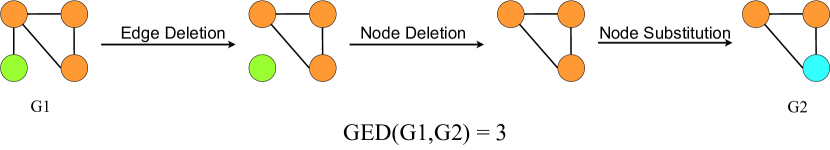
Figure 1: An edit path between graphs $\mathcal{G}_{1}$ and $\mathcal{G}_{2}$ with GED 3; the cost of each edit operation is 1.

Neural Methods: Recent works have shown that graph neural networks (GNNs) can learn a model from a training set of graph pairs and their distances to predict the GED of unseen pairs. Greed [?] employs twin GNNs with a tailored inductive bias to learn GED while preserving its metric properties. Genn-A* [?] integrates GNNs with the A* algorithm to predict distances and generate edit paths on graphs of size up to 10 nodes. H²MN [?] exploits a hierarchical hypergraph matching network to learn graph similarity. Other methods, such as SimGNN [?], GotSIM [?], and GraphSIM [?], GMN [?] also employ GNNs to estimate GED.

Nevertheless, neural approaches that approximate GED suffer from three notable drawbacks:

• Lack of interpretability: They furnish a GED between two graphs but not an edit path that entails it; such edit paths reveal crucial functions of protein complexes [?], image alignment [?], and gene-drug regulatory pathways [?].

• Restriction to small graphs: Since GED computation is NP-hard, training data are limited to small graphs, leading to lower accuracy as query size grows [?].

• Lack of generalizability: They do not generalize across datasets from different domains, as GNNs adjust to the number of unique node labels in a domain; as features change across domains, neural approximators require separate ground-truth generation and training for each data set. Coupled with the fact that training data generation is NP-hard, the pipeline is prohibitively resource-intensive.

In this paper, we present an algebraic unsupervised method called Eugene: Explainable Unsupervised Graph Edit Distance, which addresses the limitations of existing approaches for computing the Graph Edit Distance (GED), without significantly compromising on approximation accuracy. Our primary contributions are summarized as follows:

• Graph problems equivalence: We establish a fundamental connection between two pivotal graph theory problems, namely Unrestricted Graph Alignment (UGA) and Graph Edit Distance (GED), by proving that an UGA corresponds to a specific instance of GED.

• Optimization problem formulation: We cast the GED computation problem as an optimization problem over the space of all possible node alignments, represented via permutation matrices; this formulation facilitates an unsupervised solution, eschewing the need for ground-truth data generation and data-specific training.

• Interpretability with convergence guarantee: To approximate GED, Eugene minimizes a function over the set of doubly stochastic matrices, leading to a convex optimization problem that can be solved by Adam [?]. We further refine the approximation by exhorting the doubly stochastic matrix to obtain a quasi-permutation matrix form. By operating directly on matrices, Eugene yields a GED approximation explainable via a node-to-node correspondence. We also devise a customized parameter optimization strategy that guarantees convergence.

• Experimental evaluation: Our experiments demonstrate that Eugene achieves competitive accuracy on smaller graphs and outperforms the state of the art on larger graphs, while it forgoes training data and thus offers a resource-efficient, GPU-free, and therefore green computation route.

2 Notations and Preliminaries

We represent a node-labelled undirected graph as $\mathcal{G}(\mathcal{V},\mathcal{E},\mathcal{L})$ where $\mathcal{V}=[n]\equiv\{1,\ldots,n\}$ is the node set, $\mathcal{E}\subseteq[n]\times[n]$ is the edge set and $\mathcal{L}:\mathcal{V}\rightarrow\Sigma$ is a labelling function that maps nodes to labels, where $\Sigma$ is the set of all labels, including the empty label. The adjacency matrix of $\mathcal{G}$ is $A=[a_{i,j}]_{i,j\in[n]}\in\{0,1\}^{n\times n}$ such that $a_{ij}=a_{ji}=1$ if and only if $(i,j)\in E$.

Special Vectors and Matrices.

We use $\mathbf{1}$ to denote an all-ones vector, $J$ to denote an all-ones square matrix, and $O$ to denote an all-zero square matrix. We let dimensions be inferred from the employing equations.

Permutation and Doubly Stochastic Matrices.

We denote a permutation matrix of size $n$ as a binary-valued matrix $\mathbb{P}^{n}=\{P\in\{0,1\}^{n\times n}:P\mathbf{1}=\mathbf{1},P^{T}\mathbf{1}=\mathbf{1}\}$ and a doubly stochastic matrix of size $n$ as a real-valued matrix $\mathbb{W}^{n}=\{W\in[0,1]^{n\times n}:W\mathbf{1}=\mathbf{1},W^{T}\mathbf{1}=\mathbf{1}\}$.

Entry-wise Norms. Let $A\!=\![a_{ij}]_{i,j\in[n]}\!\in\!\mathbb{R}^{n\times n}$ and $p\!\in\!\mathbb{N}^{+}\cup\{\infty\}$. We define the entry-wise $p$-norm of $A$ as $\|A\|_{p}=\left(\sum_{i=1}^{n}\sum_{j=1}^{n}|a_{ij}|^{p}\right)^{\nicefrac{{1}}{{p}}}$ for $p\!\in\!\mathbb{N}+$, and $\|A\|_{\infty}\!=\!\max_{i,j}|a_{i,j}|$. We denote the entry-wise $2$-norm (i.e., the Frobenius norm) as $\|\cdot\|_{F}$.

Trace. We denote the trace of a matrix $A$ as $tr(A)$.

Graph Edit Distance (GED).

Given two graphs $\mathcal{G}_{1}$ ad $\mathcal{G}_{2}$, we define the graph edit distance between them as:

$$GED(\mathcal{G}_{1},\mathcal{G}_{2})=\min_{(e_{1},\ldots,e_{l})\in\gamma(\mathcal{G}_{1},\mathcal{G}_{2})}\sum_{i=1}^{l}c(e_{i})$$ (1)

where $\gamma(\mathcal{G}_{1},\mathcal{G}_{2})$ is the collection of all feasible edit paths that transform graph $\mathcal{G}_{1}$ into $\mathcal{G}_{2}$. The function $c(e_{i})$ corresponds to the cost assigned to edit operation $e_{i}$, where an edit can be the addition or deletion of an edge or node, or the replacement of an edge or node label. We denote a node insertion as $v_{\mathsf{ins}}(i^{\prime})$ where $i^{\prime}\in\mathcal{V(G}_{2})$ is the corresponding node in $\mathcal{G}_{2}$ . Likewise, we indicate node deletion by $v_{\mathsf{del}}(i)$ where $i\in\mathcal{V(G}_{1})$, and node substitution as $v_{\mathsf{sub}}(i,i^{\prime})$ with $i\in\mathcal{V(G}_{1})$ and $i^{\prime}\in\mathcal{V(G}_{2})$. By analogy, edge insertion $e_{\mathsf{ins}}(i^{\prime},j^{\prime})$ where $(i^{\prime},j^{\prime})\in\mathcal{E(G}_{2})$, edge deletion $e_{\mathsf{del}}(i,j)$ where $(i,j)\in\mathcal{E(G}_{1})$, and edge substitution $e_{\mathsf{sub}}(i,j,i^{\prime},j^{\prime})$ where $(i,j)\in\mathcal{E(G}_{1})$ and $(i^{\prime},j^{\prime})\in\mathcal{E(G}_{2})$, complete the defined edit operations. GED expresses the minimum cost to transform $\mathcal{G}_{1}$ to $\mathcal{G}_{2}$ over all feasible node alignments [?], an interpretation arising from the relationship between conceivable node alignments and their corresponding unique sets of edit operations. Refer to Fig. E in Appendix for examples of GED computations.

Unrestricted Graph Alignment & Chemical Distance.

The objective of unrestricted graph alignment is to identify a bijection $f:\mathcal{V(G}_{1})\rightarrow\mathcal{V(G}_{2})$ that minimizes the number of edge disagreements between the two graphs. Formally, this problem is expressed as follows:

$$\min_{P\in\mathbb{P}^{n}}\|AP-PB\|^{2}_{F},$$ (2)

where $A$ and $B$ are the adjacency matrices of graphs $\mathcal{G}_{1}$ and $\mathcal{G}_{2}$, respectively. $\mathbb{P}^{n}$ represents the set of Permutation matrices of size $n$, and $\|.\|_{F}$ denotes the Frobenius Norm. This task finds various applications, such as matching protein networks across species [?; ?], identifying users in social networks [?], and feature matching in computer vision [?; ?]. Notably, the expression in Equation 2 is the square of Chemical Distance (CD) [?] between $\mathcal{G}_{1}$ and $\mathcal{G}_{2}$.

[?] introduce the Modified Chemical Distance (MCD) that incorporates node labels. Let $\psi_{1}$ and $\psi_{2}$ be mappings that associate nodes of graphs $\mathcal{G}_{1}$ and $\mathcal{G}_{2}$, both of size $n$, to a metric space $(\Omega,d)$. Formally, $\psi_{1}:[n]\rightarrow\Omega$ and $\psi_{2}:[n]\rightarrow\Omega$. The matrix $D_{\psi_{1},\psi_{2}}$ is:

$$D_{\psi_{1},\psi_{2}}=\left[d(\psi_{1}(u),\psi_{2}(v))\right]_{u,v\in[n]}\in\mathbb{R}^{n\times n}_{+},$$ (3)

The Modified Chemical Distance (MCD) is:

$$\text{MCD}(\mathcal{G}_{1},\mathcal{G}_{2})=\min_{P\in\mathbb{P}^{n}}\|AP-PB\|_{F}+tr(P^{T}D_{\psi_{1},\psi_{2}})$$ (4)

Extending MCD to graphs of unequal sizes.

Comparing graphs of different sizes is a common need, yet the established Chemical Distance and Modified Chemical Distance metrics are limited to graphs of the same size. We extend MCD to cases where the two graphs are not of the same size, rendering it more versatile. Consider two graphs $\mathcal{G}_{1}$ and $\mathcal{G}_{2}$ with node counts $n_{1}$ and $n_{2}$, respectively ($n_{1}<n_{2}$). We augment $\mathcal{G}_{1}$ by adding $(n_{2}-n_{1})$ isolated dummy nodes, hence align the sizes of the two graphs, enabling CD and MCD calculations thereupon.

The following theorem will be useful in the following.

Theorem 1.

A doubly-stochastic matrix $A$ with $tr(A^{T}(J-A))=0$ is a permutation matrix.

Proof.

Given that $tr(A^{T}(J\!-\!A))\!=\!0$, it follows that $\sum_{i}\sum_{j}a_{ij}\cdot(1\!-\!a_{ij})\!=\!0$. Since $A$ is doubly-stochastic, $0\leq a_{ij}\leq 1$ for all $i$ and $j$, hence $a_{ij}\!\cdot\!(1\!-\!a_{ij})$ is non-negative for $1\leq i,j\leq n$. Therefore, $a_{ij}\!\cdot\!(1\!-\!a_{ij})\!=\!0$ for all $i$ and $j$. It follows that $a_{ij}$ must be either 0 or 1 for each $i$ and $j$. Considering that $A$ is doubly-stochastic and all its entries are either 0 or 1, by definition $A$ is a permutation matrix. ∎

3 Eugene: Proposed Method

Here we introduce our innovative unsupervised method that estimates the GED between a pair of graphs, $\mathcal{G}_{1}$ and $\mathcal{G}_{2}$, and also generates a comprehensible node alignment corresponding to the estimated GED. We emphasize that the GED approximated by our method is explainable, as it returns an existing edit path from graph $\mathcal{G}_{1}$ to $\mathcal{G}_{2}$ whose edit cost corresponds to the approximated GED. As the true GED is the minimum edit cost over all possible node alignments, the returned GED upper-bounds the true GED.

Our approach builds on a modified version of the Chemical distance in two stages:

• We show the objective of Unrestricted Graph Alignment, i.e., squared Chemical Distance, to be a GED instance.

• We formulate an optimization for computing a Mildly-Constrained version of GED, Mc-GED, via MCD.

Since the defined optimization problem is computationally hard, we propose two approximations that minimize the function over the space of doubly stochastic matrices $\mathbb{W}^{n}$ instead of the space of Permutation matrices $\mathbb{P}^{n}$. After obtaining the solution from the approximations, we convert it into a permutation matrix that represents a valid node alignment by one of two methods, Greedy and Hungarian. Lastly, we output the generated permutation matrix defining the node alignment to which the approximated GED corresponds.

3.1 Unrestricted Graph Alignment & GED

We now prove that an Unrestricted Graph Alignment corresponds to an instance of GED. We show that by expressing the square of the Chemical distance between two graphs $\mathcal{G}_{1}$ and $\mathcal{G}_{2}$, defined in Equation (2), as an instance of GED. Consider an instance of GED between graphs $\mathcal{G}_{1}$ and $\mathcal{G}_{2}$ whose adjacency matrices are $A,B$ respectively, where the cost of edit operations is defined as follows:

• Node insertion cost = 0

• Node deletion cost = 0

• Node substitution cost = 0

• Edge insertion cost = 2

• Edge deletion cost = 2

• Edge substitution cost = 0

We show that the GED between $\mathcal{G}_{1}$ and $\mathcal{G}_{2}$ by these edit costs is equal to the square of their Chemical Distance.

Lemma 1.

Given graphs $\mathcal{G}_{1}$, $\mathcal{G}_{2}$ of size $n$ and a node alignment function $p:[n]\rightarrow[n]$ mapping each node $i$ in $\mathcal{G}_{1}$ to a node $p(i)$ in $\mathcal{G}_{2}$, the edit distance corresponding to the node alignment by the aforementioned edit costs is equal to $\|AP-PB\|^{2}_{F}$, where $P$ is a permutation matrix with $P_{ij}=1$ if $p(i)=j$, otherwise 0.

Proof.

Let $\mathcal{E}_{ins}$ be the set of edges inserted in $\mathcal{G}_{1}$ and $\mathcal{E}_{del}$ that of edges deleted by alignment $p$, where without loss of generality an edge $(i,j)$ has $i<j$. As node edits and edge substitutions cost zero, the edit distance $\text{ED}(p)$ is:

$$\text{ED($p$)}=\sum_{\mathclap{(i,j)\in\mathcal{E}_{ins}}}c(e_{\mathsf{ins}}(p(i),p(j)))+\sum_{\mathclap{(i,j)\in\mathcal{E}_{del}}}c(e_{\mathsf{del}}(i,j))$$

In this expression, $c(e_{\mathsf{ins}}(p(i),p(j)))$ and $c(e_{\mathsf{del}}(i,j))$ denote the costs of edge insertion and deletion between nodes $i$ and $j$, respectively. By the defined costs, we get:

$$\text{ED($p$)}=\sum_{(i,j)\in\mathcal{E}_{ins}}2+\sum_{(i,j)\in\mathcal{E}_{del}}2\\$$

We note that, if an edge between nodes $i$ and $j$ requires insertion, then $a_{ij}=0$ and $b_{p(i)p(j)}=1$, as it does not exist in $A$ but exists in $B$. Likewise, an edge that needs deletion has $a_{ij}=1$ and $b_{p(i)p(j)}=0$. For all other pairs $(i,j)$, it is $a_{ij}=b_{p(i)p(j)}$. Consequently, we obtain:

$$\text{ED($p$)}=\sum_{\mathclap{(i,j)\in\mathcal{E}_{ins}}}2\cdot(a_{ij}-b_{p(i)p(j)})^{2}+\sum_{\mathclap{(i,j)\in\mathcal{E}_{del}}}2\cdot(a_{ij}-b_{p(i)p(j)})^{2}+0$$

Further manipulation yields:

$$\begin{split}\text{ED($p$)}=\sum_{\mathclap{(i,j)\in\mathcal{E}_{ins}}}(a_{ij}-b_{p(i)p(j)})^{2}+(a_{ji}-b_{p(j)p(i)})^{2}+\\ \sum_{\mathclap{(i,j)\in\mathcal{E}_{del}}}(a_{ij}-b_{p(i)p(j)})^{2}+(a_{ji}-b_{p(j)p(i)})^{2}+\\ \sum_{\mathclap{i<j\wedge(i,j)\in[n]\times[n]\setminus(\mathcal{E}_{del}\cup\mathcal{E}_{ins})}}(a_{ij}-b_{p(i)p(j)})^{2}+(a_{ji}-b_{p(j)p(i)})^{2}\\ \end{split}$$

$$\text{Consequently, ED($p$)}=\sum_{\mathclap{(i,j)\in[n]\times[n]}}(a_{ij}-b_{p(i)p(j)})^{2}=$$

$$\|A-PBP^{T}\|^{2}_{F}=\|AP-PB\|^{2}_{F}$$

∎

Lemma 2.

Given two graphs $\mathcal{G}_{1}$ and $\mathcal{G}_{2}$ of size $n$, GED($\mathcal{G}_{1}$, $\mathcal{G}_{2}$) = CD($\mathcal{G}_{1}$, $\mathcal{G}_{2}$)², with GED computed by the above costs.

Proof.

By Lemma 1, ED($p$) = $\|AP-PB\|^{2}$. It is GED = $\min_{p}$ ED($p$) = $\min_{P\in\mathbb{P}^{n}}$ $\|AP-PB\|^{2}$, since there is a one-to-one mapping between alignment functions $p$ and permutation matrices $P$; then GED($\mathcal{G}_{1}$, $\mathcal{G}_{2}$) = CD($\mathcal{G}_{1}$, $\mathcal{G}_{2}$)². ∎

The preceding lemmata establish squared Chemical Distance (CD)² as an instance of Graph Edit Distance (GED). From Equation 2 it follows that the objective of Unrestricted Graph Alignment is an instance of GED.

3.2 Closed form for mildly-constrained GED

We consider a mildly-constrained version of GED, Mc-GED, between node-labeled graphs $\mathcal{G}_{1}$ and $\mathcal{G}_{2}$ of sizes $n_{1},n_{2}$ respectively, with the following edit costs:

• Node insertion cost = $c(v_{\mathsf{ins}}(j))$, where $j\in\mathcal{V(G}_{2})$.

• Node deletion cost = $c(v_{\mathsf{del}}(i))$, where $i\in\mathcal{V(G}_{1})$.

• Node substitution cost = $c(v_{\mathsf{sub}}(i,j))$, where $i\in\mathcal{V(G}_{1})$ and $j\in\mathcal{V(G}_{2})$.

• Edge insertion cost = $k^{2}$

• Edge deletion cost = $k^{2}$

• Edge substitution is an operation we do not allow.

where $c$ can be any arbitrary cost function and $k$ is a scalar. Under these mildly constrained edit costs, we propose a closed-form expression that utilizes the concept of Modified Chemical Distance MCD, as introduced in Eq. (4):

$$\min_{P\in\mathbb{P}^{n}}\frac{||\tilde{A}P-P\tilde{B}||_{F}^{2}}{2}+tr(P^{T}D)$$ (5)

Let $A,B$ be adjacency matrices of graphs $\mathcal{G}_{1}$, $\mathcal{G}_{2}$ respectively, after extending the smaller graph to the size of larger graph by adding isolated dummy nodes. Then we set $\tilde{A}=k.A,\tilde{B}=k.B$ and define $D$ as follows:

$$d_{ij}=\begin{cases}c(v_{\mathsf{ins}}(j)),&\text{if }i\text{ is a dummy node in }\mathcal{G}_{1}\\ c(v_{\mathsf{del}}(i)),&\text{if }j\text{ is a dummy node in }\mathcal{G}_{2}\\ c(v_{\mathsf{sub}}(i,j)),&\text{otherwise}\end{cases}$$

We show that, with $\tilde{A},\tilde{B},D$ defined as above, the distance in Equation (5) equals the mildly-constrained GED.

Lemma 3.

Given two graphs $\mathcal{G}_{1}$, $\mathcal{G}_{2}$ of size $n$ whose adjacency matrices are $A,B$ respectively, a constant $k$ where $k^{2}$ is the edge insertion and deletion cost, matrix $D$ as defined above and a permutation matrix $P$, $\frac{||\tilde{A}P-P\tilde{B}||_{F}^{2}}{2}+tr(P^{T}D)$ equals the mildly-constrained edit distance (Mc-ED) by the above specified edit costs, for node alignment $p:[n]\rightarrow[n]$, where $p(i)=j$ if and only if $P_{ij}=1$.

Proof.

We evaluate the given expression:

$$\frac{||\tilde{A}P-P\tilde{B}||_{F}^{2}}{2}+tr(P^{T}D)=\frac{||\tilde{A}-P\tilde{B}P^{T}||_{F}^{2}}{2}+tr(P^{T}D)\\$$

Using the node-alignment function $p$, we reformulate the above equation to:

$$\sum_{\mathclap{(i,j)\in[n]\times[n]}}k^{2}\cdot\frac{(a_{ij}-b_{p(i)p(j)})^{2}}{2}+\sum_{i\in[n]}d_{i,p(i)}$$

Further manipulation via the definition of matrix $D$ gives:

$$\begin{split}\sum_{\mathclap{(i,j)\in[n]\times[n]}}k^{2}\cdot\frac{(a_{ij}-b_{p(i)p(j)})^{2}}{2}+\sum_{\mathclap{i\in\mathcal{G}_{1}\text{is a dummy node}}}c(v_{\mathsf{ins}}(p(i)))+\\ \sum_{\mathclap{i\in\mathcal{G}_{1}\text{is mapped to dummy node}}}c(v_{\mathsf{del}}(i))+\sum_{i\in\mathcal{G}_{1}\text{otherwise}}c(v_{\mathsf{sub}}(i,p(i)))\end{split}$$

We observe that, for any $(i,j)\in[n]\times[n]$, if $a_{ij}=0$ and $b_{p(i)p(j)}=1$, an edge should be inserted between nodes $(i,j)$. Likewise, if $a_{ij}=1$ and $b_{p(i)p(j)}=0$, an edge between $(i,j)$ should be deleted. On the other hand, if $a_{ij}=b_{p(i)p(j)}$, the corresponding term evaluates to 0 and can be disregarded. Moreover, a node $i$ in $\mathcal{G}_{1}$ designated as a dummy node should be inserted with $p(i)$ serving as the corresponding node in $\mathcal{G}_{2}$. Similarly, a node $i$ mapped to a dummy node $p(i)$ should be deleted. In the event that none of these conditions apply, node $i$ is substituted with node $p(i)$. Consequently, the expression can be further simplified as:

$$\begin{split}\sum_{\mathclap{(i,j)\text{ inserted}}}k^{2}\cdot\frac{b_{p(i)p(j)}^{2}+b_{p(j)p(i)}^{2}}{2}+\sum_{\mathclap{(i,j)\text{ deleted}}}k^{2}\cdot\frac{a_{ij}^{2}+a_{ji}^{2}}{2}+\\ \sum_{\mathclap{i\in\mathcal{G}_{1}\text{ inserted}}}c(v_{\mathsf{ins}}(p(i)))+\sum_{\mathclap{i\in\mathcal{G}_{1}\text{ deleted}}}c(v_{\mathsf{del}}(i))+\!\!\!\!\!\!\!\sum_{i\in\mathcal{G}_{1}\text{otherwise}}\!\!\!\!\!\!\!\!c(v_{\mathsf{sub}}(i,p(i)))\end{split}$$

Substituting the values, we yield:

$$\begin{split}\sum_{(i,j)\text{ inserted}}k^{2}+\sum_{(i,j)\text{ deleted}}k^{2}+\sum_{(i,j)\text{ is substituted}}0+\\ \sum_{\mathclap{i\in\mathcal{G}_{1}\text{ inserted}}}c(v_{\mathsf{ins}}(p(i)))+\sum_{\mathclap{i\in\mathcal{G}_{1}\text{ deleted}}}c(v_{\mathsf{del}}(i))+\!\!\!\!\!\!\!\sum_{i\in\mathcal{G}_{1}\text{otherwise}}\!\!\!\!\!\!\!\!\!c(v_{\mathsf{sub}}(i,p(i)))\end{split}$$

This result is the Mc-ED matching node alignment $p$. ∎

Lemma 4.

For graphs $\mathcal{G}_{1}$ and $\mathcal{G}_{2}$ of size $n$, the distance by Equation (5) equals the Mc-GED between $\mathcal{G}_{1}$ and $\mathcal{G}_{2}$.

Proof.

By Lemma 3, $\frac{||\tilde{A}P-P\tilde{B}||_{F}^{2}}{2}+tr(P^{T}D)$ equals Mc-ED($p$), hence $\min_{P\in\mathbb{P}^{n}}\frac{||\tilde{A}P-P\tilde{B}||_{F}^{2}}{2}+tr(P^{T}D)$ corresponds to $\min_{p}$ Mc-ED($p$) due to the one-to-one mapping between $p$ and $P$. Thus, the distance computed by Equation (5) is the Mc-GED between $\mathcal{G}_{1}$ and $\mathcal{G}_{2}$. ∎

3.3 Approximating Mc-GED

While Equation (5) offers a closed-form expression for Mc-GED, finding the permutation matrix that minimizes this expression is notoriously hard, as the space of permutation matrices is not convex. Here, we relax this optimization problem to approximate the Mc-GED by expanding the optimization domain from the discrete space of permutation matrices to the more tractable space of doubly stochastic matrices, and then guide the solution towards a quasi-permutation matrix.

[?] show how to find the minimal Chemical Distance over the set of doubly stochastic matrices $\mathbb{W}^{n}$ instead of the more restrictive set of permutation matrices $\mathbb{P}^{n}$. Similarly, we solve the optimization problem in Equation (5) over the domain of $\mathbb{W}^{n}$, rendering it convex, as it aims to minimize a convex function over a convex domain [?]; the problem becomes:

$$\begin{gathered}\min_{P}\frac{||AP-PB||_{F}^{2}}{2}+tr(P^{T}D)\\ \text{Constraints: }P\textbf{1}=\textbf{1},P^{T}\textbf{1}=\textbf{1},0\leq P_{ij}\leq 1\end{gathered}$$ (6)

We apply the Adam algorithm [?] to this convex problem to obtain a doubly stochastic matrix, yet restrict the solution to a quasi-permutation matrix. By Theorem 1, if $P$ is doubly-stochastic and $tr(P^{T}(J-P)$ = 0, then $P$ is a permutation matrix. We rewrite the expression to find mildly-constrained GED in Equation (5) as:

$$\begin{gathered}\min_{P\in\mathbb{W}^{n}}\frac{||AP-PB||_{F}^{2}}{2}+tr(P^{T}D)\\ \text{Constraints: }tr(P^{T}(J-P))=0\end{gathered}$$ (7)

We introduce parameters $\mu$ and $\lambda$ and relax further to:

$$\begin{gathered}\min_{P}\!\frac{||A\!P\!-\!P\!B||_{F}^{2}}{2}\!+\!\mu(tr(P^{T}\!D))+\lambda(tr(P^{T}\!(J\!-\!P)))\\ \text{Constraints: }P\textbf{1}\!=\!P^{T}\textbf{1}\!=\!\textbf{1},0\!\leq\!P_{ij}\!\leq\!1\end{gathered}$$ (8)

For $\lambda$ = 0, this problem is convex. To find a quasi-permutation matrix, we first solve Equation (8) with $\lambda$ = 0 using Adam, and further refine the solution by gradually increasing $\lambda$, until it diverges. This Modified-Adam (M-Adam) algorithm, presented in Algorithm 1, yields a quasi-permutation matrix.

Algorithm 1 M-Adam

Notations:
$f=\frac{||AP-PB||_{F}^{2}}{2}+\mu*(tr(P^{T}D))$
$g=tr(P^{T}(J-P))$
$pnlt=||P\textbf{1}-\textbf{1}||^{2}+||P^{T}\textbf{1}-\textbf{1}||^{2}+||max(0,-P)||^{2}+||max(0,P-J)||^{2}$
$\sigma$ is the penalty-coefficient
Input: A, B, D
Output: $P$
Algorithm:

  $P\leftarrow I$, $\sigma\leftarrow 10$,$\lambda\leftarrow 0$, $m_{0}\leftarrow 0$, $v_{0}\leftarrow 0$, $\beta_{1}\leftarrow 0.9$, $\beta_{2}\leftarrow 0.99$

  while true do

     $t\leftarrow 0$

     while not converged do

        $t\leftarrow t+1$

        $\textit{grad}\leftarrow\nabla f+\sigma*\nabla pnlt+\lambda*\nabla g$

        $m_{t}\leftarrow\beta_{1}\cdot m_{t-1}+(1-\beta_{1})\cdot grad$

        $v_{t}\leftarrow\beta_{2}\cdot v_{t-1}+(1-\beta_{2})\cdot grad^{2}$

        $\hat{m_{t}}\leftarrow m_{t}/(1-\beta_{1}^{t})$

        $\hat{v_{t}}\leftarrow v_{t}/(1-\beta_{2}^{t})$

        $P\leftarrow P-\alpha\cdot\hat{m_{t}}/(\sqrt{\hat{v_{t}}}+\epsilon)$

        $\lambda\leftarrow max(0,\lambda-\delta)$

     if diverged then

        break

     $\sigma\leftarrow\sigma*10$

     $\lambda\leftarrow\lambda+0.5$

     if $\sigma>\sigma_{th}$ then

        break

  return  $P$

Theorem 2.

Algorithm 1 converges in finite time.

Proof.

Assume the algorithm does not converge for some value of $\lambda$. Then it must be stuck in the inner $\mathrm{while}$ loop of Algorithm 1. Each iteration of that loop subtracts a fixed positive $\delta$ from $\lambda$. In effect, $\lambda$ reaches 0 after finite iterations and remains unchanged thereafter, while the inner $\mathrm{while}$ loop minimizes a convex function, terminating in finite steps. Therefore, the algorithm converges in finite time. ∎

3.4 Rounding Algorithms

M-Adam yields a quasi-permutation matrix. However, we need a permutation matrix to derive an edit path. We apply two algorithms to round these matrices denoted as $A$ to a permutation matrix $P$: Greedy and Hungarian.

Greedy: In each iteration, if permutation matrix constraints allow, we set the largest unvisited entry in the input matrix to 1, else 0, until we visit all entries. Algorithm 2 in the appendix shows the pseudocode, following [?].

Hungarian: As with Greedy, we construe the rounding problem as an assignment problem, seeking an 1-to-1 mapping from the nodes of $\mathcal{G}_{1}$ to those of $\mathcal{G}_{2}$ that maximizes the sum of selected input matrix entries $A_{ij}$, and find the optimal solution by the Hungarian algorithm [?].

Both Greedy and Hungarian serve as heuristics. We choose, among the two outputs, the one that yields lower edit cost, hence nears the GED cost. Efficiency-wise, we prefer Greedy, which is lighter and still offers a fine alignment.

4 Experiments

In this section, we benchmark Eugene against state-of-the-art GED approximators and establish that it: (1) outperforms competitors in accuracy, especially on large graph datasets; (2) incurs significantly lower computation cost than neural algorithms, which take up to 17 days to generate training data and require GPU access; and (3) enjoys scalability to large graphs even while being independent of supervision data.

Our C++ code and datasets are available at https://anonymous.4open.science/r/EUGENE-1107/.

4.1 Experimental Setup

All experiments ran on a machine equipped with an Intel Xeon Gold 6142 CPU @1GHz and a GeForce GTX 1080 Ti GPU. While non-neural methods including Eugene run on the CPU, neural baselines exploit the GPU.

Table 1: Datasets.

Name	# Graphs	Avg $|\mathcal{V}|$	Avg $|\mathcal{E}|$	# labels	Domain
ogbg-molhiv	39650	24	52	119	Biology
ogbg-molpcba	436313	26	56	119	Biology
ogbg-code2	139468	37	72	97	Software
AIDS	700	9	9	29	Biology
Linux	1000	8	7	NA	Software
IMDB	1500	13	65	NA	Movies

Datasets: Table 1 presents the datasets used and their characteristics. Appendix D provides details on dataset semantics. While OGBG data [?] are large graph repositories, the remaining three comprise comparatively smaller graphs. We consider graphs of fewer than 50 nodes in OGBG.

Baselines: We benchmark Eugene against the state-of-the-art baselines of Greed [?], H²MN [?], Genn-A* [?], and SimGNN [?]. We train these models by the settings their authors recommend and use the codebase they shared. We list the parameters for Eugene in Appendix C. We exclude the neural approximation algorithms of GraphSim [?], GMN [?] and [?], as Greed and H²MN have shown vastly better performance [?; ?]. Among neural methods, only Genn-A* [?] furnishes a node alignment that entails the predicted GED.

In the unsupervised category, we compare to the GEDlib implementation [?] of Branch [?], known for its even accuracy-time tradeoff, which navigates the search space via the linear sum assignment problem with error-correction (LSAPE).

Train-Validation-Test Split: From each dataset, we select 1K graph pairs uniformly at random and compute true edit distances to form a test set. The train set comprises 100K graph pairs and the validation set comprises 10K graph pairs with their true GEDs, drawn uniformly at random from the graph set on condition that they do not appear in the test set and contain at most 25 nodes. We introduce the second constraint because computing the true GED is NP-hard and hence prohibitively expensive. As we discuss in detail later, computing true GEDs for 100K graphs containing up to 25 nodes took 16 and 17 days in ogbg-molhiv and ogbg-molpcba, respectively. We employ Mip-F2 [?] to generate ground truth GED.

4.2 Accuracy

Tables 2(a)–2(b) present approximation accuracy results in terms of Root-Mean-Squared-Error (RMSE) on large and small datasets. A pattern emerges; while Eugene performs best on large graphs (Table 2(a)), Greed marginally outperforms Eugene on smaller graphs (Table 2(b)). Eugene’s performance on large graphs highlights its scalability with respect to graph size and GED value. Furthermore, Eugene and Greed are the only algorithms featured among top-3 performers across all datasets. Genn-A* does not scale to graphs exceeding $10$ nodes and hence is listed only with AIDS and Linux.

Table 2: Accuracy Comparison (RMSE) among baselines. The top-3 lowest RMSEs in each dataset is highlighted in various shades of green with darker shades indicating lower RMSE (better).

(a) RMSE on large datasets.

Methods	ogbg-molhiv	ogbg-molpcba	ogbg-code2
Eugene	2.93	2.98	3.22
Greed	3.02	2.48	5.52
H2MN	12.01	5.50	11.96
SimGNN	10.04	4.01	21.52
Branch	9.86	11.31	12.64

(b) RMSE on small datasets.

Methods	AIDS	Linux	IMDB
Eugene	0.83	0.46	12.2
Greed	0.61	0.41	4.8
H2MN	1.14	0.60	57.8
Genn-A*	0.85	0.47	NA
SimGNN	1.11	0.74	159.1
Branch	3.31	2.45	7.35

Performance on larger graphs

While Table 2(a) highlights Eugene’s edge on large graphs, we next evaluate larger graphs. As the acquisition of training data for GED learning is resource-intensive due to the NP-hardness of GED computations, neural approaches need to train on smaller graphs and apply the acquired knowledge to larger graphs of previously unseen sizes. We examine the extent of this generalization ability for Greed and H²MN, trained on $100k$ graphs of size less than $25$ extracted from OGBG datasets and evaluated on graphs of sizes in the range $[25,50]$. Table 3 presents the outcomes. Eugene exhibits superior performance compared to both Greed and H²MN when confronted with previously unseen graph sizes, underscoring its practical applicability on large graphs.

Table 3: Accuracy Comparison (RMSE) of Eugene with Greed, H²MN over large graphs of previously unseen size.

Methods	ogbg-molhiv	ogbg-molpcba	ogbg-code2
Eugene	3.50	2.99	2.68
Greed	6.01	6.86	4.71
H2MN	23.00	22.12	16.67

Impact of Query Size and GED

Next, we examine the generalizability of neural approaches on graphs of seen size, i.e., within 25 nodes. The task complexity rises with graph size due to the exponential growth of mappings in combinatorial space. Figs. 2–4 present heatmaps of RMSE vs. query graph size and true GED value on ogbg-molhiv, ogbg-molpcba, and ogbg-code2 data. Each point on the plot indicates a query graph $\mathcal{G}_{Q}$ with coordinates (GED($\mathcal{G}_{Q}$, $\mathcal{G}_{T}$), $|\mathcal{V}_{Q}|$), where $\mathcal{G}_{T}$ is a fixed target graph. Heatmaps for Greed present a discernibly darker tone across the spectrum than those for Eugene. Moreover, darker shades are more pronounced in the upper and right portions, implying a deterioration in performance as query sizes and GED values rise. We infer that Eugene enjoys greater scalability with respect to query sizes and GED values. We show heatmaps for H²MN in Appendix E.

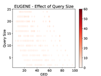
(a)

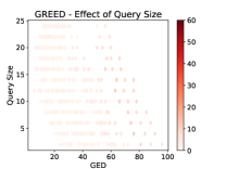
(b)

Figure 2: RMSE heatmap vs. query size & GED, ogbg-molhiv.

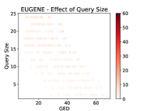
(a)

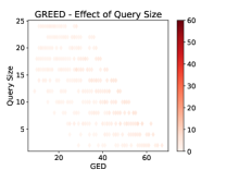
(b)

Figure 3: RMSE heatmap vs. query size & GED, ogbg-molpcba.

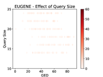
(a)

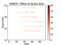
(b)

Figure 4: RMSE heatmap vs. query size & GED, ogbg-code2.

4.3 Efficiency

Table 4 lists running times on ogbg-molhiv, ogbg-molpcba, and ogbg-code2, including ground truth generation, training, and inference for $1000$ query pairs. We relegate running time for small data (AIDS, Linux, IMDB) to Appendix E and omit SimGNN and Branch due to their much weaker performance. Even while neural models benefit from GPU acceleration and abstain from providing an edit path, Eugene, working on the CPU, is much faster. While the inference time of neural models may seem advantageous, our holistic evaluation including training reveals that Eugene is more efficient. Ground truth generation, which exceeded 16 days on ogbg-molhiv and ogbg-molpcba and $\sim$1 day on ogbg-code2, constrains the usability of neural models to these datasets. Further, despite their resource-intensive training process, Eugene surpasses the accuracy of neural methods on ogbg-molhiv and ogbg-code2 and ranks second on ogbg-molpcba. Appendix E itemizes Eugene’s computation costs.

Table 4: Running times (HH:MM:SS) on three data sets.

(a) ogbg-molhiv

Methods	Ground Truth Time	Training	Inference
Eugene	-	-	00:06:06
Greed	379:19:35	01:07:36	00:00:02
H2MN	379:19:35	02:00:03	00:00:02

(b) ogbg-molpcba

Methods	Ground Truth Time	Training	Inference
Eugene	-	-	00:06:36
Greed	414:30:54	01:48:07	00:00:02
H2MN	414:30:54	02:10:57	00:00:01

(c) ogbg-code2

Methods	Ground Truth Time	Training	Inference
Eugene	-	-	00:07:57
Greed	21:42:31	02:29:08	00:00:02
H2MN	21:42:31	02:20:06	00:00:02

4.4 Transferability

As Section 4.3 establishes ground-truth generation as the primary bottleneck of neural algorithms, the question arises: Can neural algorithms train on a data set of small graphs and transfer that knowledge to larger graphs, thereby circumventing the generation of dataset-specific expensive ground-truth data? We next examine this transferability question.

Table 5: Transfer Learning (off-diagonal) – Greed (RMSE); diagonals show cases of train and test sets drawn from the same dataset. We relegate the transferability analysis for H²MN to Appendix E.

	Train Set			Eugene
Test Set	AIDS	ogbg-molhiv	ogbg-molpcba
AIDS	0.61	5.71	4.58	0.83
ogbg-molhiv	NA	3.02	3.86	2.93
ogbg-molpcba	NA	2.16	2.48	2.98

First, as discussed in § 1, transferability is not feasible across datasets characterized by different features. This happens since the number of parameters in a GNN is a function of the feature dimension. Thus, we specifically examine transferability across chemical compound datasets. We train the neural model on one dataset and subsequently test it on test sets of other datasets. Since the AIDS dataset contains only 29 unique labels (chemical elements), transferability from AIDS to other chemical datasets, which contain $119$ unique elements, is not feasible. Table 5 shows RMSE scores for transfer learning using Greed, juxtaposed to those of Eugene on the same test sets. Except one case highlighted in yellow, we observe a significant drop in accuracy across all other transfer learning scenarios. The fact that Eugene generally outperforms Greed even without exploiting any training information further corroborates its robustness.

4.5 Summary: Eugene vs. Greed

The cost of ground truth generation limits the applicability of Greed on large-graph datasets, on which Eugene emerges as the unequivocally preferable method. On small-graph datasets, Greed remains remarkably competitive. In effect, the choice between Greed and Eugene should weigh a marginal increase in accuracy on smaller-graph datasets against interpretability and the bypassing of NP-hard ground-truth instance generation and costly training on each dataset.

4.6 Ablation Study

We have hitherto examined the performance of Eugene, which drives a doubly stochastic matrix toward a quasi-permutation matrix before rounding. Here, we introduce a variant, Eugene’, which directly rounds the doubly stochastic matrix to a permutation matrix. Table 6 shows RMSE values for Eugene and Eugene’. Eugene achieves substantially higher accuracy, underscoring the efficacy of refining Eugene’s solution toward a quasi-permutation matrix.

Table 6: Accuracy (RMSE), Eugene vs. Eugene’.

Datasets	Eugene	Eugene’
ogbg-molhiv	2.93	12.66
ogbg-molpcba	2.98	13.35
ogbg-code2	3.22	7.02
AIDS	0.83	3.29
Linux	0.46	2.34
IMDB	12.2	13.5

5 Conclusions and Future work

We introduced Eugene, an unsupervised method that explainably estimates Graph Edit Distance (GED) grounded on an algebraic representation and a relaxation of the ensuing optimization followed by rounding. Through extensive comparative analysis, we demonstrated the effectiveness of Eugene in estimating GED and underscored its capacity to match and even exceed the performance of neural supervised methods. Moreover, thanks to its unsupervised nature, Eugene eschews the need to generate supervisory data via NP-hard computations and train models tailored to specific datasets. These characteristics render Eugene a choice candidate for practical applications in graph similarity measurement, pattern recognition, and network analysis. As our implementation only utilizes CPU resources, forgoing the advantages of GPU acceleration, it is open to future enhancements. Looking ahead, we aspire to extend the scope of our method to encompass graph alignment tasks that transcend GED estimation.

6 Appendix

A GED Computation

Figure E shows the GED computation among five graphs using Equation (1) where each edit operation costs 1.

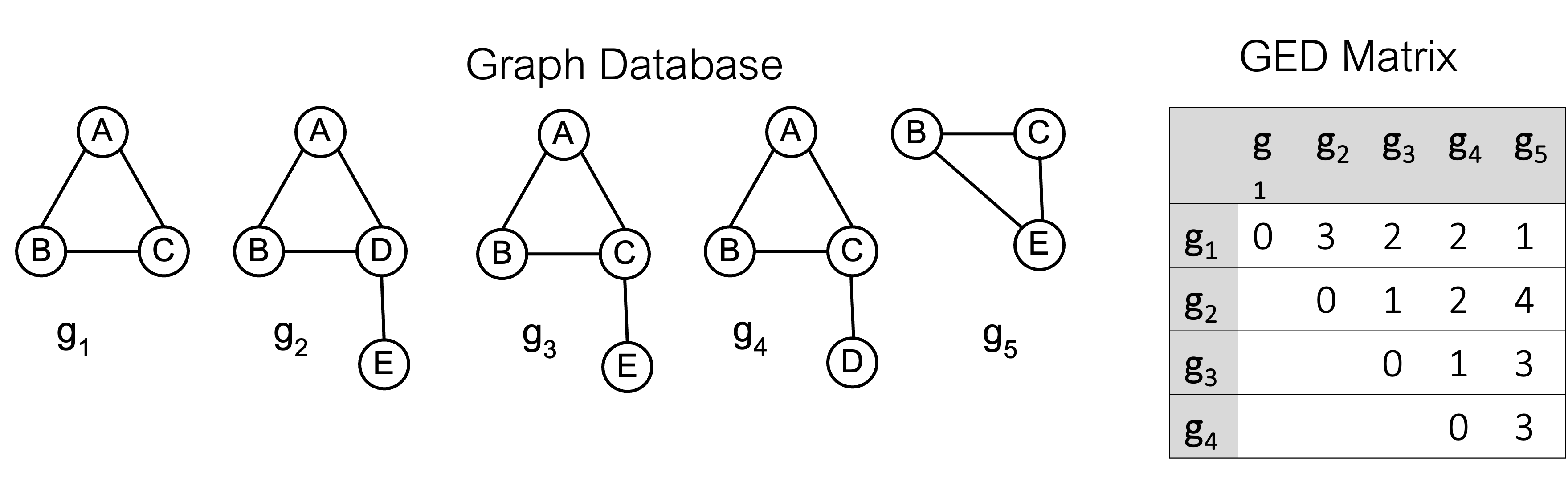
Figure E: GED among five graphs; all edit operations cost 1.

B Rounding Algorithm - Greedy

Algorithm 2 lists the pseudocode for the Greedy rounding algorithm that converts a matrix $A$ to a permutation matrix $P$.

Algorithm 2 Greedy

Input: $A$
Output: $P$

  $P\leftarrow O$

  $visited\leftarrow empty$

  while $\text{not all indices in }A\text{ are visited}$ do

     $(i,j)\leftarrow\text{non-visited }(row,col)\text{ with highest entry in A}$

     if $\text{1 is not present in row }i\text{, column }j$ then

        $P(i,j)\leftarrow 1$

     $visited(i,j)\leftarrow true$

  return  $P$

C Parameters

Table G lists the parameters used for Eugene. We set the convergence criterion of M-Adam to $abs(prev\_dist-cur\_dist)<1e^{-7}$, where $prev\_dist,cur\_dist$ are the approximated Graph edit distances in two successive iterations, $itr-1$ and $itr$.

Table G: Parameters used in Eugene.

parameter	value
$\mu$	0.1
$\delta$	$1e^{-6}$
$\alpha$	0.001
$\sigma_{th}$	$1e^{4}$

D Datasets

Here we present the semantics of the datasets we used.

• AIDS: A compilation of graphs originating from the AIDS antiviral screen database, which represents chemical compound structures. The graphs in this dataset possess sizes not exceeding 10 nodes. Graphs in this dataset are labelled.

• Linux: A collection of program dependence graphs wherein nodes correspond to statements and edges indicate dependencies between statements. The graph sizes in this dataset also remain below or equal to 10 nodes. This dataset was introduced in [?]. Graphs in this dataset are un-labelled.

• IMDB: Comprising ego-networks of actors/actresses who have shared screen time in movies. This was introduced in [?]. Graphs in this dataset are un-labelled.

• ogbg-molhiv, ogbg-molpcba: These are chemical compound datasets of different sizes, each graph represents a molecule, wherein nodes correspond to atoms and edges represent chemical bonds. The atomic number of the respective atom serves as the node label.

• ogbg-code2: A collection of Abstract Syntax Trees (ASTs) obtained from approximately 450 thousands Python method definitions. Each node in the AST is assigned a label from a set of 97 labels. We considered the graphs as undirected.

E Experiments

Metrics

RMSE: Evaluates the prediction accuracy by measuring the disparities between actual and predicted values. For $n$ graph pairs, it is defined as:

$$\sqrt{\frac{1}{n}\sum_{i=1}^{n}(\text{true-ged}_{i}-\text{pred-ged}_{i})^{2}}$$ (9)

Test Data

The statistics of the test data used for the evaluation of Eugene are presented in Table. H.

Table H: Test data stats.

Name	# Graph pairs	Avg $|\mathcal{V}|$	Avg $|\mathcal{E}|$
AIDS	1000	8.8	8.8
Linux	1000	7.6	7
IMDB	967	12.2	57
ogbg-molhiv	902	23	49.5
ogbg-molpcba	859	25	54.1
ogbg-code2	968	36.7	35.7

Efficiency (Small Datasets)

Table. I present a runtime comparison of Eugene with Greed, H²MN, and Genn-A* on small datasets. The results demonstrate the superior performance of Eugene when compared to neural methods. Despite the reduced time requirements for ground-truth generation in comparison to OGBG datasets, it remains notably high, exceeding 5 days for the IMDB dataset. We also note the significant disparity in computational speed between Eugene and Genn-A*, a neural model that also offers node alignment capability. Eugene demonstrates superior efficiency, notably outperforming Genn-A* in terms of processing time. Genn-A* does not scale to graphs exceeding 10 nodes and hence is listed only with AIDS and Linux.

Table I: Running times (HH:MM:SS) on small data sets.

(a) AIDS

Methods	Ground Truth Time	Training	Inference
Eugene	-	-	00:02:59
Genn-A*	09:43:28	07:28:35	02:31:29
Greed	09:43:28	01:01:28	00:00:02
H2MN	09:43:28	01:50:45	00:00:02

(b) Linux

Methods	Ground Truth Time	Training	Inference
Eugene	-	-	00:02:58
Genn-A*	03:25:26	00:59:10	00:15:49
Greed	03:25:26	01:29:05	00:00:03
H2MN	03:25:26	02:09:56	00:00:01

(c) IMDB

Methods	Ground Truth Time	Training	Inference
Eugene	-	-	00:09:21
Greed	124:25:47	01:09:40	00:00:03
H2MN	124:25:47	02:59:53	00:00:01

Transferability

Table J presents the RMSE scores for transfer learning using H²MN, comapred with Eugene on the same test sets. Similar to Greed, we observed significant drop in accuracy in all transfer learning scenarios except one case highlighted in yellow. It is essential to highlight that Eugene consistently outperforms H²MN across all test sets by a significant margin.

Table J: Transfer Learning (off-diagonal) – H²MN (RMSE); diagonals show cases of train and test sets drawn from the same dataset.

	Train Set			Eugene
Test Set	AIDS	ogbg-molhiv	ogbg-molpcba
AIDS	1.14	3.61	2.90	0.83
ogbg-molhiv	NA	12.01	11.01	2.93
ogbg-molpcba	NA	5.95	5.50	2.98

Impact of Query Size and GED

The heatmaps illustrating the impact of Query Size and GED for H²MN across seen graph sizes for OGBG datasets are delineated in Fig. F, the corresponding representations for Eugene and Greed are already detailed in §. 4.2. A discernible trend emerges as the heatmaps for H²MN exhibit markedly darker tones in comparison to Eugene, indicative of its suboptimal scalability with Query Size and GED even within seen graph sizes.

Subsequently, we examine the influence of Query Size and GED for unseen graph sizes i.e., more than 25 nodes. Figs. G–I depict Heatmaps of RMSE vs. query graph size and true GED values for the ogbg-molhiv, ogbg-molpcba, and ogbg-code2 datasets. The visual analysis reveals a pronounced darkening in the heatmaps corresponding to Greed and H²MN in contrast to Eugene. Additionally, a discernible lack of scalability with respect to query size and GED is noted for Greed and H²MN, while Eugene exhibits superior scalability in these contexts.

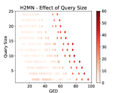
(a)

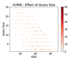
(b)

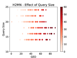
(c)

Figure F: Heatmap for variation of RMSE with Query Size - H²MN on ogbg-molhiv, ogbg-molpcba, ogbg-code2 datasets.

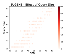
(a)

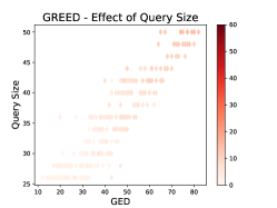
(b)

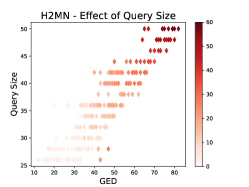
(c)

Figure G: Heatmap for variation of RMSE with Query Graph Size - Eugene vs Greed vs H²MN on ogbg-molhiv dataset

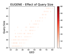
(a)

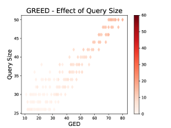
(b)

(c)

Figure H: Heatmap for variation of RMSE with Query Graph Size - Eugene vs Greed vs H²MN on ogbg-molpcba dataset

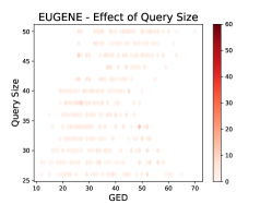
(a)

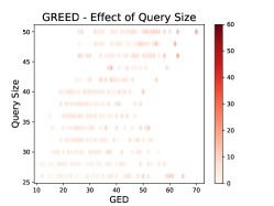
(b)

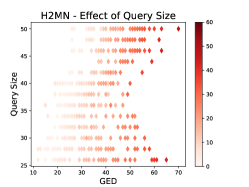
(c)

Figure I: Heatmap for variation of RMSE with Query Graph Size - Eugene vs Greed vs H²MN on ogbg-code2 dataset

Comparison of rounding algorithms

Table K juxtaposes the two rounding algorithms, Greedy and Hungarian, used to transform a quasi-permutation matrix to a permutation matrix, on the datasets sets of Table 1, counting instances where they yield the same GED and those where one outperforms the other. While Hungarian has a slight advantage, we recommend using Greedy in view of its efficiency.

Table K: Analysis of Rounding Algorithms.

Name	Greedy best	Hungarian best	Same cost	Total Pairs
AIDS	3	7	990	1000
Linux	0	13	987	1000
IMDB	20	110	837	967
ogbg-molhiv	18	78	806	902
ogbg-molpcba	22	63	774	859
ogbg-code2	36	116	816	968

Component-wise analysis of Eugene

The time efficiency of Eugene is scrutinized in the context of two key stages: the optimization of Eq. 8, and the subsequent rounding of the derived quasi-permutation matrix. Table  L presents the time consumption per graph pair. Optimization constitutes the major bottleneck, while rounding is much quicker. Notably, processing ogbg and IMDB graphs takes longer due to their higher density compared to those in AIDS and Linux data.

Table L: Component-wise runtime (msec) per graph pair, Eugene.

Datasets	Optimization	Rounding
AIDS	6978	2
Linux	6237	2
IMDB	22508	16
ogbg-molhiv	26411	35
ogbg-molpcba	24213	30
ogbg-code2	27435	67

References

- [Bai et al., 2019] Yunsheng Bai, Hao Ding, Song Bian, Ting Chen, Yizhou Sun, and Wei Wang. Simgnn: A neural network approach to fast graph similarity computation. In WSDM, WSDM ’19, page 384–392, 2019.
- [Bai et al., 2020] Yunsheng Bai, Hao Ding, Ken Gu, Yizhou Sun, and Wei Wang. Learning-based efficient graph similarity computation via multi-scale convolutional set matching. AAAI, pages 3219–3226, Apr. 2020.
- [Bento and Ioannidis, 2018] José Bento and Stratis Ioannidis. A family of tractable graph distances. In Proceedings of the SIAM International Conference on Data Mining, SDM, pages 333–341, 2018.
- [Blumenthal and Gamper, 2020] David B Blumenthal and Johann Gamper. On the exact computation of the graph edit distance. Pattern Recognition Letters, 134:46–57, 2020.
- [Blumenthal et al., 2019a] David B. Blumenthal, Nicolas Boria, Johann Gamper, Sébastien Bougleux, and Luc Brun. Comparing heuristics for graph edit distance computation. The VLDB Journal, 29(1):419–458, jul 2019.
- [Blumenthal et al., 2019b] David B Blumenthal, Sébastien Bougleux, Johann Gamper, and Luc Brun. Gedlib: a c++ library for graph edit distance computation. In International Workshop on Graph-Based Representations in Pattern Recognition, pages 14–24. Springer, 2019.
- [Boyd and Vandenberghe, 2004] Stephen Boyd and Lieven Vandenberghe. Convex optimization. Cambridge university press, 2004.
- [Chang et al., 2020] Lijun Chang, Xing Feng, Xuemin Lin, Lu Qin, Wenjie Zhang, and Dian Ouyang. Speeding up ged verification for graph similarity search. In 2020 IEEE 36th International Conference on Data Engineering (ICDE), pages 793–804, 2020.
- [Chen et al., 2018] Jiazhou Chen, Hong Peng, Guoqiang Han, Hongmin Cai, and Jiulun Cai. HOGMMNC: a higher order graph matching with multiple network constraints model for gene–drug regulatory modules identification. Bioinformatics, 35(4):602–610, 07 2018.
- [Conte et al., 2003] D. Conte, P. Foggia, C. Sansone, and M. Vento. Graph matching applications in pattern recognition and image processing. In Proceedings 2003 International Conference on Image Processing (Cat. No.03CH37429), volume 2, pages II–21, 2003.
- [Cordella et al., 2004] L.P. Cordella, P. Foggia, C. Sansone, and M. Vento. A (sub)graph isomorphism algorithm for matching large graphs. IEEE Transactions on Pattern Analysis and Machine Intelligence, 26(10):1367–1372, 2004.
- [Doan et al., 2021] Khoa D. Doan, Saurav Manchanda, Suchismit Mahapatra, and Chandan K. Reddy. Interpretable graph similarity computation via differentiable optimal alignment of node embeddings. In SIGIR, page 665–674, 2021.
- [Doka et al., 2015] Katerina Doka, Mingqiang Xue, Dimitrios Tsoumakos, and Panagiotis Karras. -anonymization by freeform generalization. In ASIACCS, pages 519–530, 2015.
- [Hu et al., 2020] Weihua Hu, Matthias Fey, Marinka Zitnik, Yuxiao Dong, Hongyu Ren, Bowen Liu, Michele Catasta, and Jure Leskovec. Open graph benchmark: Datasets for machine learning on graphs. In H. Larochelle, M. Ranzato, R. Hadsell, M.F. Balcan, and H. Lin, editors, Advances in Neural Information Processing Systems, volume 33, pages 22118–22133. Curran Associates, Inc., 2020.
- [Kazemi et al., 2015] Ehsan Kazemi, S. Hamed Hassani, and Matthias Grossglauser. Growing a graph matching from a handful of seeds. Proc. VLDB Endow., 8(10):1010–1021, jun 2015.
- [Kingma and Ba, 2015] Diederik P. Kingma and Jimmy Ba. Adam: A method for stochastic optimization. In 3rd International Conference on Learning Representations, ICLR, 2015.
- [Kuhn, 1955] H. W. Kuhn. The Hungarian method for the assignment problem. Naval Research Logistics Quarterly, 2(1–2):83–97, 1955.
- [Kvasnicka et al., 1991] Vladimir Kvasnicka, Jiri Pospíchal, and Vladimír Baláž. Reaction and chemical distances and reaction graphs. Theoretica chimica acta, 79:65–79, 1991.
- [Lerouge et al., 2017a] Julien Lerouge, Zeina Abu-Aisheh, Romain Raveaux, Pierre Héroux, and Sébastien Adam. New binary linear programming formulation to compute the graph edit distance. Pattern Recognition, 72:254–265, 2017.
- [Lerouge et al., 2017b] Julien Lerouge, Zeina Abu-Aisheh, Romain Raveaux, Pierre Héroux, and Sébastien Adam. New binary linear programming formulation to compute the graph edit distance. Pattern Recognition, 72:254–265, 2017.
- [Li et al., 2019] Yujia Li, Chenjie Gu, Thomas Dullien, Oriol Vinyals, and Pushmeet Kohli. Graph matching networks for learning the similarity of graph structured objects. In ICML, pages 3835–3845, 2019.
- [Lin, 1994] Chih-Long Lin. Hardness of approximating graph transformation problem. In International Symposium on Algorithms and Computation, 1994.
- [Ranjan et al., 2022] Rishabh Ranjan, Siddharth Grover, Sourav Medya, Venkatesan Chakaravarthy, Yogish Sabharwal, and Sayan Ranu. Greed: A neural framework for learning graph distance functions. In Advances in Neural Information Processing Systems 36: Annual Conference on Neural Information Processing Systems 2022, NeurIPS 2022, November 29-Decemer 1, 2022, 2022.
- [Riesen and Bunke, 2009] Kaspar Riesen and Horst Bunke. Approximate graph edit distance computation by means of bipartite graph matching. Image and Vision Computing, 27:950–959, 06 2009.
- [Riesen et al., 2007] Kaspar Riesen, Stefan Fankhauser, and Horst Bunke. Speeding up graph edit distance computation with a bipartite heuristic. 01 2007.
- [Sharan and Ideker, 2006] Roded Sharan and Trey Ideker. Modeling cellular machinery through biological network comparison. Nature biotechnology, 24:427–33, 05 2006.
- [Singh et al., 2008] Rohit Singh, Jinbo Xu, and Bonnie Berger. Global alignment of multiple protein interaction networks with application to functional orthology detection. Proceedings of the National Academy of Sciences, 105(35):12763–12768, 2008.
- [Wang et al., 2012] Xiaoli Wang, Xiaofeng Ding, Anthony K. H. Tung, Shanshan Ying, and Hai Jin. An efficient graph indexing method. In Proceedings of the 2012 IEEE 28th International Conference on Data Engineering, ICDE ’12, page 210–221, USA, 2012. IEEE Computer Society.
- [Wang et al., 2021] Runzhong Wang, Tianqi Zhang, Tianshu Yu, Junchi Yan, and Xiaokang Yang. Combinatorial learning of graph edit distance via dynamic embedding. In IEEE Conference on Computer Vision and Pattern Recognition, 2021.
- [Yanardag and Vishwanathan, 2015] Pinar Yanardag and S.V.N. Vishwanathan. Deep graph kernels. In Proceedings of the 21th ACM SIGKDD International Conference on Knowledge Discovery and Data Mining, KDD ’15, page 1365–1374, New York, NY, USA, 2015. Association for Computing Machinery.
- [Zeng et al., 2009] Zhiping Zeng, Anthony Tung, Jianyong Wang, Jianhua Feng, and Lizhu Zhou. Comparing stars: On approximating graph edit distance. PVLDB, 2:25–36, 01 2009.
- [Zhang et al., 2021] Zhen Zhang, Jiajun Bu, Martin Ester, Zhao Li, Chengwei Yao, Zhi Yu, and Can Wang. H2mn: Graph similarity learning with hierarchical hypergraph matching networks. In KDD, page 2274–2284, 2021.