You’ve Got to Feel It To Believe It: Multi-Modal Bayesian Inference for Semantic and Property Prediction

Abstract

Robots must be able to understand their surroundings to perform complex tasks in challenging environments and many of these complex tasks require estimates of physical properties such as friction or weight. Estimating such properties using learning is challenging due to the large amounts of labelled data required for training and the difficulty of updating these learned models online at run time. To overcome these challenges, this paper introduces a novel, multi-modal approach for representing semantic predictions and physical property estimates jointly in a probabilistic manner. By using conjugate pairs, the proposed method enables closed-form Bayesian updates given visual and tactile measurements without requiring additional training data. The efficacy of the proposed algorithm is demonstrated through several hardware experiments. In particular, this paper illustrates that by conditioning semantic classifications on physical properties, the proposed method quantitatively outperforms state-of-the-art semantic classification methods that rely on vision alone. To further illustrate its utility, the proposed method is used in several applications including to represent affordance-based properties probabilistically and a challenging terrain traversal task using a legged robot. In the latter task, the proposed method represents the coefficient of friction of the terrain probabilistically, which enables the use of an on-line risk-aware planner that switches the legged robot from a dynamic gait to a static, stable gait when the expected value of the coefficient of friction falls below a given threshold. Videos of these case studies as well as the open-source C++ and ROS interface can be found at https://roahmlab.github.io/multimodal_mapping/.

I Introduction

Scene understanding from exteroceptive sensing via images or point clouds enables mobile robots to perform object avoidance, terrain traversal, and a variety of other tasks. The introduction of high-level and task-dependent semantic labels for scene understanding has recently spurred rapid growth in this area [1, 2]. To extract semantic labels from images or point clouds, it is common to employ semantic segmentation neural networks; however, even state-of-the-art methods return inconsistent labels under viewpoint or lighting changes, and are heavily reliant on the data used for training. Unfortunately, collecting data to train these networks is expensive and out-of-distribution examples may lead to incorrect classifications.

To address the challenge of viewpoint inconsistency, several state-of-the-art methods project image-based semantic classifications onto metric maps [3, 4]. This provides a shared frame of reference between images thereby enabling the application of probabilistic methods to fuse semantic data. While such methods demonstrate improved performance over state-of-the-art image-based segmentation [5], these methods have been restricted to either visual or lidar data. This is limiting since the properties of a semantic class are often of primary interest rather than the class labels themselves while completing a robotic task. For instance, the coefficient of friction is more informative than the terrain class for a legged robot. While recent semantic mapping methods have derived recursive filters for image-based semantic predictions, properties conditioned on these semantic classes are often assumed to be known a priori and are considered immutable at run time [6, 5, 3].

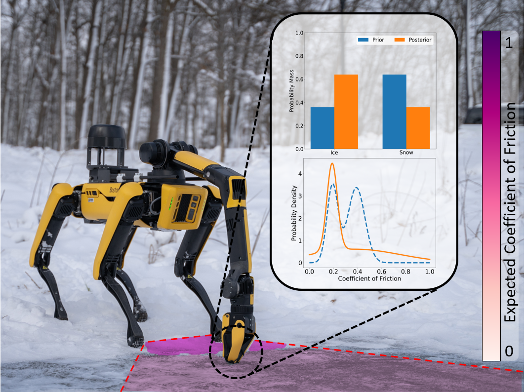
Figure 1: The method proposed in this paper jointly estimates semantic classifications and physical properties by combining visual and tactile data into a single semantic mapping framework. RGB-D images are used to build a metric-semantic map that iteratively estimates semantic labels. A property measurement is taken which in turn updates both the semantic class predictions and physical property estimates. In the depicted example, the robot is unsure if the terrain in front of it is snow or ice from vision measurements alone (prior estimates) which dramatically affects the coefficient of friction and the associated gait that can be applied to safely traverse the terrain. The robot uses a tactile sensor attached to its manipulator to update its coefficient of friction estimation (posterior estimates), which then enables it to change gaits to cross the ice safely.

This paper introduces a multi-modal semantic prediction and property estimation framework to jointly estimate semantic labels alongside physical properties as depicted in Figure 1. The key insight is that semantic classifications may be conditioned on their physical properties and physical properties may likewise be conditioned on their semantic classifications. In this way, vision-based semantic classifications can be used to build a measurement model for physical properties, and tactile-based sensing can be used to update the semantic predictions via property measurements. To apply this insight, this paper demonstrates how to recursively estimate physical properties from semantic class predictions using only visual information. Subsequently, this paper describes how to exploit a tactile sensing modality to update the semantic classification and property estimates probabilistically and in closed-form using Bayesian inference.

The efficacy of the proposed approach is demonstrated on several hardware platforms including a robotic manipulator and a legged robot. First, we show that by leveraging friction measurements obtained through tactile sensing we can improve semantic classification performance when compared to state-of-the-art semantic mapping methods that rely solely on visual information. Second, we demonstrate that our approach estimates physical properties more accurately than a method using vision alone. Multiple sensing modalities are used to estimate the coefficient of friction of the terrain surrounding a robot, which enables the use of an online risk-aware planner that switches the legged robot from a dynamic gait to a static, stable gait if the expected value of the coefficient of friction of the terrain falls below a given threshold. Importantly, the proposed multi-modal framework allows the legged robotic system to complete a challenging terrain traversal task whereas state-of-the-art vision-based traversability estimation methods fail to accurately predict the traversability of the terrain resulting in the robot slipping and falling. Finally, we show the broad applicability of the proposed framework for affordance-based property prediction by demonstrating door opening with unknown push-pull interactions.

The contribution of this work is the introduction of a probabilistic model for jointly estimating semantic classifications and physical properties. This enables closed-form Bayesian updates given visual semantic classifications and tactile property measurements. We demonstrate that by leveraging this probabilistic approach, we are able to improve semantic prediction accuracy by an average of $21.3\%$ in simulation using only one property measurement. These results are validated in hardware demonstrations. Two case studies are subsequently presented that illustrate the utility of performing this type of multi-modal property estimation. An open-source C++ and ROS package for the robot-agnostic implementation of the proposed approach as well as videos of the case studies are provided on the project page website.

The remainder of this paper is organized as follows: Section II summarizes the semantic prediction and property estimation literature and Section III reviews preliminary material used throughout the paper. Section IV provides an overview of our method. Section V introduces the vision-based semantic prediction pipeline and Section VI the tactile-based semantic prediction and property estimation pipeline. Section VII describes the implementation. Sections VIII and IX describe the evaluation of our algorithm in simulation and using hardware demonstrations, respectively. Section X discusses future work and provides concluding remarks.

II Related Works

This section describes related work in semantic prediction and property estimation as well as the gap in the literature this work addresses.

II-A Semantic Prediction

State-of-the-art methods for semantic classification almost exclusively rely on neural networks to produce pixel-wise semantic predictions [1, 7, 8]. Often these approaches use task-dependent object designations as semantic labels [9, 10] such as abstract topological information [11] or material classifications [12]. Unfortunately, semantic prediction methods often have no temporal consistency, meaning two subsequent images in a video stream may have vastly different semantic predictions.

To overcome this challenge and relate semantic predictions spatially and temporally, early work in semantic mapping projected semantic predictions onto a geometric representation forming a metric-semantic map [13]. In this way, image-based semantic predictions have a shared frame of reference within this map. These early methods employed voting-like schemes, regularization, and other algorithmic methods to fuse semantic predictions [4, 14].

Recent work in semantic mapping treats the semantic fusion process probabilistically to recursively estimate semantic labels [3, 15]. These methods treat pixel-wise semantic predictions as measurements and probabilistically fuse these measurements over the map using Bayesian inference. By approaching semantic prediction in this way, these approaches are robust to noisy pixel-wise semantic classifications and have been shown to be more accurate than methods that rely on image-based classifications alone [5].

Multi-modal semantic prediction, and the corresponding semantic mapping extension, have been around since the rise of modern computer vision [16]. Much of this work comes from the vision community and, as such, many of these methods rely on different vision-based modalities such as depth [17], thermal imaging [18], and scale-invariant feature transform (SIFT) factors [19]. Many modern multi-modal semantic classification methods are learning-based, where the multi-modal visual features are combined either at the input of or downstream within neural networks to output semantic classifications [20, 21].

II-B Property Estimation

While semantic classification methods have seen widespread use in the robotics community, there are many robotic tasks (e.g., footstep planning, grasp planning, manipulation) where the underlying physical properties of the semantic classes are critical. Additionally, if semantic classifications are incorrect, the resultant property estimates may also be incorrect, leading to task failure.

Previous work in property estimation has focused on estimating the expected value for the coefficient of friction from vision alone [22, 23, 24]. These methods have been extended in a recent paper that estimates probability distributions for the coefficient of friction given visual semantic class estimates by conditioning properties on semantic classes [5].

Other methods for property estimation focus specifically on estimating traversability [3, 25]. This is done to bypass the need to estimate terrain properties by instead estimating the regions in the environment a robot can traverse using visual features [26]. This is often an ill-posed problem as traversability is not only terrain-dependent, but also dependent on the motion of the robot (e.g., walking vs. running) [27]. For example, it is possible for small insects to walk across a large body of water, but if a large robot applied the same gait it would most likely sink.

Notably, there has been a recent shift towards multi-modal property estimation in the literature. One such approach proposes an online, self-supervised learning framework to estimate traversability by back-projecting previously traversed regions into the camera frame and training a network in a self-supervised manner to correctly label these previously seen regions as traversable [28]. This method is considered multi-modal because it incorporates an implicit goal-success signal, in the form of the robot having not fallen over, alongside visual information. Other work aims to encode property features in a latent space using tactile and visual information to train reinforcement learning agents [29]. Recently, [30] proposed a method for learning motion policies by training a network to relate image-based features and physical properties such as friction in simulation. It was shown that the trained network accurately predicted properties in hardware demonstrations, however these predictions only output a single scalar value for properties without considering uncertainty in the prediction. A similar framework for multi-modal probabilistic property estimation within a semantic mapping framework was also demonstrated for the purposes of traversability estimation [6]. In this case, the terrain classes are modelled probabilistically using Dirichlet distributions (analogous to [5, 3]) and trained networks are then used to predict the likelihood of slipping using data collected offline.

II-C Gap in the Literature

The methods discussed in the prior two subsections have two notable shortcomings. The first is that, while existing property estimation algorithms condition physical properties on semantic classifications, this conditioning of properties is immutable, meaning the property values of semantic classes cannot be updated during operation [6, 5, 3]. This is undesirable especially when such physical properties have intra-class variation or there are errors in these initial estimates. For example, the coefficient of friction of ice depends on the conditions of ice formation, outdoor temperature, and the presence of snow on the surface of the ice. Assuming that the coefficient of all ice is identical may result in unsafe or overly conservative behavior.

The second short-coming of these methods is the one-way conditioning of physical properties on semantic classes. This can be unduly limiting because visual information alone may not be sufficiently informative. For example, in Fig. 1 it is challenging to differentiate between snow and ice from just an RGB sensor. Using a tactile sensor in this instance to estimate the friction coefficient can inform and improve the accuracy of the semantic classification. Using physical properties to inform semantic classification can enable the application of multiple sensing modalities while providing a means of verification for semantic predictions output by trained networks. This improves the accuracy of semantic predictions without requiring new training data and network retraining.

To address these short-comings, this paper proposes a method to jointly estimate semantic classifications and physical properties online using Bayesian inference. Semantic classifications from vision enable the prediction of physical properties, and tactile measurements enable the online update of physical property estimates. This in turn enables the semantic classification likelihoods to be updated.

III Preliminaries

This section introduces notation, moments, and conjugate pairs. Vectors, written as columns, are typeset in bold and lowercase, while sets and matrices are typeset in uppercase. The element $i$ of a vector $\bm{x}$ is denoted as $x_{i}$. An n-dimensional closed interval is denoted by $[a,b]^{n}$. Let $p$ denote a normalized probability mass or density function. Following the convention of [31], we distinguish between different probability mass or density functions by the variable used as an input argument into each $p$.

III-A Conjugate Pairs

In probability, conjugate distributions are a pair of distributions such that, given a prior and a likelihood, the posterior computed using Bayes’ theorem belongs to the same family of distributions as the prior [32]. This enables tractable computation of closed-form solutions for the posterior [33]. We introduce two such conjugate pairs here: the Dirichlet and Categorical distributions, and the Dirichlet Normal-Inverse-Gamma product and Gaussian mixture distributions.

III-A1 First Conjugate Pair

Let $z\in\{1,\ldots,k\}$ denote a discrete random variable. The probability mass function of the Categorical distribution represents the probability that a sample $z$ belongs to class $i$:

$$p(z=i|\bm{\theta})=Cat(z=i|\bm{\theta})=\theta_{i},$$ (1)

where $i\in\{1,2,\dots,k\}$, $\bm{\theta}\in[0,1]^{k}$, and $\sum_{i}\theta_{i}=1$.

The Dirichlet distribution is a continuous k-variate probability distribution that is parameterized by a vector $\bm{\alpha}\in\mathbb{R}^{k}_{\geq 0}$ with probability density:

$$p(\bm{\theta}|\bm{\alpha}) =Dir(\bm{\theta}|\bm{\alpha})$$ (2)

$$=\frac{\Gamma(\sum_{j=1}^{k}\alpha_{j})}{\sum_{j=1}^{k}\Gamma(\alpha_{j})}\prod_{j=1}^{k}\theta_{j}^{\alpha_{j}-1},$$ (3)

where

$$\Gamma(\alpha_{j})=\int_{0}^{\infty}x^{\alpha_{j}-1}\exp(-x)dx.$$ (4)

The Dirichlet distribution is a conjugate prior to the Categorical distribution as is formalized in the following theorem whose proof is provided in Appendix A:

Theorem 1.

Let $\mathcal{Z}=\{z_{1},\dots,z_{n}\}$ be a set of measurements drawn from a Categorical distribution, $p(z_{j}=i|\bm{\theta})$, and let the prior for $\bm{\theta}$ be a Dirichlet distribution, $p(\bm{\theta}|\bm{\alpha})$. The posterior computed using Bayes’ theorem, $p(\bm{\theta}|\mathcal{Z},\bm{\alpha})$, is also a Dirichlet distribution such that:

$$p(\bm{\theta}|\mathcal{Z},\bm{\alpha})=Dir(\bm{\theta}|\tilde{\bm{\alpha}}),$$ (5)

where

$$\tilde{\alpha}_{j} =\alpha_{j}+\sum_{z_{i}\in\mathcal{Z}}1\{z_{i}=j\},$$ (6)

and $1\{z_{i}=j\}$ is equal to $1$ when the expected class of measurement $z_{i}$ is class $j$ and is zero otherwise.

Theorem 1 enables the computation of the predictive posterior. In particular, one of the goals of this paper is to predict the probability that a new measurement belongs to class $i$ given prior measurements $\mathcal{Z}$:

$$p(z=i|\mathcal{Z},\bm{\alpha}) =p(z=i|\tilde{\bm{\alpha}})$$ (7)

$$=\int_{\bm{\theta}}p(z=i|\bm{\theta})p(\bm{\theta}|\tilde{\bm{\alpha}})\text{d}\theta,$$ (8)

where $p(z=i|\bm{\theta})$ represents the Categorical likelihood and $p(\bm{\theta}|\tilde{\bm{\alpha}})$ the Dirichlet posterior probability. Computing this integral exactly is challenging. Fortunately, the theory of conjugate priors enables a closed-form solution [34, (3)]:

$$p(z=i|\tilde{\bm{\alpha}})=\frac{\tilde{\alpha}_{i}}{\sum_{j=1}^{k}\tilde{\alpha}_{j}}.$$ (9)

III-A2 Second Conjugate Pair

Let $\psi\in\mathbb{R}$ denote a continuous random variable. A Gaussian mixture is a continuous probability density function

$$p(\psi|\Theta)=\sum_{i=1}^{k}w_{i}\mathcal{N}(\psi|\mu_{i},\sigma_{i}^{2}),$$ (10)

where $\Theta=\{w_{i},\mu_{i},\sigma_{i}^{2}\}_{i=1}^{k}$ and $\sum_{i=1}^{k}w_{i}=1$. Next, we present a candidate for the conjugate prior of the Gaussian mixture model by conditioning the parameters, $\Theta$, on a set of hyperparameters, $\Psi$. Previously, the Dirichlet distribution was used to parameterize these variables to form a conjugate pair. We perform a similar trick here using the Dirichlet Normal-Inverse-Gamma product distribution as the prior on $\Theta$.

The Dirichlet Normal-Inverse-Gamma product distribution is defined as

$$p(\Theta|\Psi)=Dir(\bm{w}|\bm{a})\prod_{i=1}^{k}\mathcal{NIG}(\mu_{i},\sigma^{2}_{i}|\tau_{i},\kappa_{i},\beta_{i},\gamma_{i}),$$ (11)

where $\Psi=\{a_{i},\tau_{i},\kappa_{i},\beta_{i},\gamma_{i}\}_{i=1}^{k}$, $\kappa_{i},\beta_{i},\gamma_{i}>0$, and the Normal-Inverse-Gamma distribution is defined as

$$\mathcal{NIG}(\mu_{i},\sigma_{i}^{2}|\tau_{i},\kappa_{i},\beta_{i},\gamma_{i}) =\frac{\sqrt{\kappa_{i}}}{\sqrt{2\pi\sigma_{i}^{2}}}\frac{\gamma_{i}^{\beta_{i}}}{\Gamma(\beta_{i})}\frac{1}{\sigma_{i}^{2}}^{\beta_{i}+1}\cdot$$ (12)

$$\cdot\exp(-\frac{2\gamma_{i}+\kappa_{i}(x-\tau_{i})^{2}}{2\sigma_{i}^{2}}).$$

When a measurement $\psi$ is taken, we assume it is drawn from the Gaussian mixture measurement likelihood. The posterior of $\Theta$ is then computed using the following theorem from [35, (6)]:

Theorem 2.

Let $\psi$ be a measurement drawn from a Gaussian mixture $p(\psi|\Theta)$. Let the prior for $\Theta$ be a Dirichlet Normal-Inverse-Gamma product distribution. Then the posterior computed using Bayes’ theorem, $p(\bm{\theta}|\psi,\Psi)$, is:

$$p(\Theta|\psi,\Psi)=\frac{1}{M}\sum_{j=1}^{k} c_{j}Dir(\bm{w}|\tilde{\bm{a}}_{j})\cdot$$

$$\cdot\mathcal{NIG}(\mu_{j},\sigma^{2}_{j}|\tilde{\tau}_{j},\tilde{\kappa}_{j},\tilde{\beta}_{j},\tilde{\gamma}_{j})\cdot$$

$$\cdot\prod_{i\neq j}^{k}\mathcal{NIG}(\mu_{i},\sigma^{2}_{i}|\tau_{i},\kappa_{i},\beta_{i},\gamma_{i}),$$ (13)

where

$$\tilde{a_{j}} =a_{j}+1,$$ (14)

$$\tilde{\tau_{j}} =\frac{\kappa_{j}\tau_{j}+\psi}{\kappa_{j}+1},$$ (15)

$$\tilde{\kappa_{j}} =\kappa_{j}+1,$$ (16)

$$\tilde{\beta_{j}} =\beta_{j}+\frac{1}{2},$$ (17)

$$\tilde{\gamma_{j}} =\gamma_{j}+\kappa_{j}\frac{(\psi-\tau_{j})^{2}}{2(1+\kappa_{j})},$$ (18)

$$c_{j} =\sqrt{\frac{\kappa_{j}}{\tilde{\kappa_{j}}}}\frac{\Gamma(\tilde{\beta}_{j})}{\Gamma(\beta_{j})}\frac{{\gamma_{j}}^{(\beta_{j})}}{{\tilde{\gamma}_{j}}^{(\tilde{\beta}_{j})}},$$ (19)

$\tilde{\bm{a}}_{j}=\{a_{1},\ldots a_{j-1},\tilde{a}_{j},a_{j+1},\ldots,a_{k}\}$ and $M$ is the normalizing factor.

Using Theorem 2, note the posterior, (2), is not in the same family of distributions as the prior, (11). More troublingly, the number of terms in (2) grows exponentially with the number of measurements. Rather than apply Theorem 2, we implement the method of moments described in the next section to approximate (2) as a Dirichlet Normal-Inverse-Gamma product distribution.

III-B Method of Moments

Let $\bm{\lambda}=\{\lambda_{1},\ldots,\lambda_{n}\}$ be an n-dimensional continuous random variable with probability density function $p(\bm{\lambda}|\xi)$ conditioned on parameters $\xi$. The $i$-th order moment is defined as

$$M_{g_{i}(\bm{\lambda})}(p)=\mathbb{E}[g_{i}(\bm{\lambda})]$$ (20)

where $g_{i}$ is a monomial of $\bm{\lambda}$ of degree $i$. For some distributions, there exists a finite set of such moments, termed the sufficient moments [35] that fully define the set of parameters $\xi$. This means that one can construct the probability density function for this distribution by just using the sufficient moments. We denote the set of sufficient moments of a distribution $p$ as $\mathbb{S}_{p}$.

The method of moments is a technique that fits a distribution to a set of sampled data by matching the sufficient moments of the distribution with the empirical moments computed from data. This approach may also be used to approximate a distribution by another distribution in a different family of distributions by matching sufficient moments of the first distribution with those of the second distribution. For our purposes, we use the method of moments to approximate the posterior computed using Theorem 2 with a probability density from the family of Dirichlet Normal-Inverse-Gamma product distributions. This may be thought of as projecting the first distribution onto the family of the second distribution [35]. This process is summarized in Algorithm 1 for projecting (2) onto the family of distributions of (11).

1

Requires : Dataset $\mathcal{D}=\{\psi_{l}\}_{l=1}^{N}$, Prior $p(\Theta|\Psi)$

2 for $\psi\in\mathcal{D}$ do

       Compute $p(\Theta|\psi,\Psi)$// (2)

       $\mathbb{E}[g_{j}(\bm{\theta})]\leftarrow$ moments($p(\Theta|\psi,\Psi)$) // (20)

       $\hat{\Psi}\leftarrow$ matchMoments() // (22)-(26)

3       Compute $p(\Theta|\hat{\Psi})$

Algorithm 1 Method of Moments

III-C Revisiting the Dirichlet Normal-Inverse-Gamma Product

By implementing Algorithm 1, we project (2) onto the family of Dirichlet Normal-Inverse-Gamma product distributions resulting in an approximate posterior. To compute this projection using the method of moments, we first need the sufficient moments of the Dirichlet Normal-Inverse-Gamma product distribution. From [35, §4.1], these sufficient moments are $\mathbb{S}_{p}=\{\mu_{i},\sigma^{2}_{i},\sigma_{i}^{4},\mu_{i}^{2}\sigma^{2}_{i},w_{i},w_{i}^{2}\}_{i=1}^{k}$. This process is summarized in the following theorem whose proof is given in Appendix B:

Theorem 3.

Let $\psi$ be a measurement drawn from a Gaussian mixture $p(\psi|\Theta)$. Let the prior for $\Theta$ be a Dirichlet Normal-Inverse-Gamma product distribution. Then the posterior computed using Bayes’ theorem, $p(\bm{\theta}|\psi,\Psi)$, and projected onto the family of Dirichlet Normal-Inverse-Gamma product distributions via Algorithm 1 yields:

$$p(\Theta|\hat{\Psi})=Dir(\bm{w}|\hat{\bm{a}})\prod_{i=1}^{k}\mathcal{NIG}(\mu_{i},\sigma^{2}_{i}|\hat{\tau}_{i},\hat{\kappa}_{i},\hat{\beta}_{i},\hat{\gamma}_{i}).$$ (21)

The parameters $\hat{\Psi}$ are computed using the sufficient moments of (2):

$$\hat{\tau_{i}} =\mathbb{E}[\mu_{i}],$$ (22)

$$\hat{\kappa_{i}} =\frac{1}{\mathbb{E}[\mu_{i}^{2}\sigma^{2}_{i}]-\mathbb{E}[\mu_{i}]^{2}\mathbb{E}[\sigma^{2}_{i}]},$$ (23)

$$\hat{\beta_{i}} =\frac{\mathbb{E}[\sigma^{2}_{i}]^{2}}{\mathbb{E}[\sigma_{i}^{4}]-\mathbb{E}[\sigma^{2}_{i}]^{2}},$$ (24)

$$\hat{\gamma_{i}} =\frac{\mathbb{E}[\sigma^{2}_{i}]}{\mathbb{E}[\sigma_{i}^{4}]-\mathbb{E}[\sigma^{2}_{i}]^{2}},$$ (25)

$$\hat{a_{i}} =\mathbb{E}[w_{i}]\frac{\mathbb{E}[w_{i}]-\mathbb{E}[w_{i}^{2}]}{\mathbb{E}[w_{i}^{2}]-\mathbb{E}[w_{i}]^{2}}.$$ (26)

Theorem 3 is applied sequentially when multiple measurements are given. We summarize this procedure in Algorithm 1. The posterior predictive distribution is then given as $p(\psi|\hat{\Theta})$, which is a Gaussian mixture, where $\hat{\Theta}=\mathbb{E}[p(\Theta|\hat{\Psi})]$.

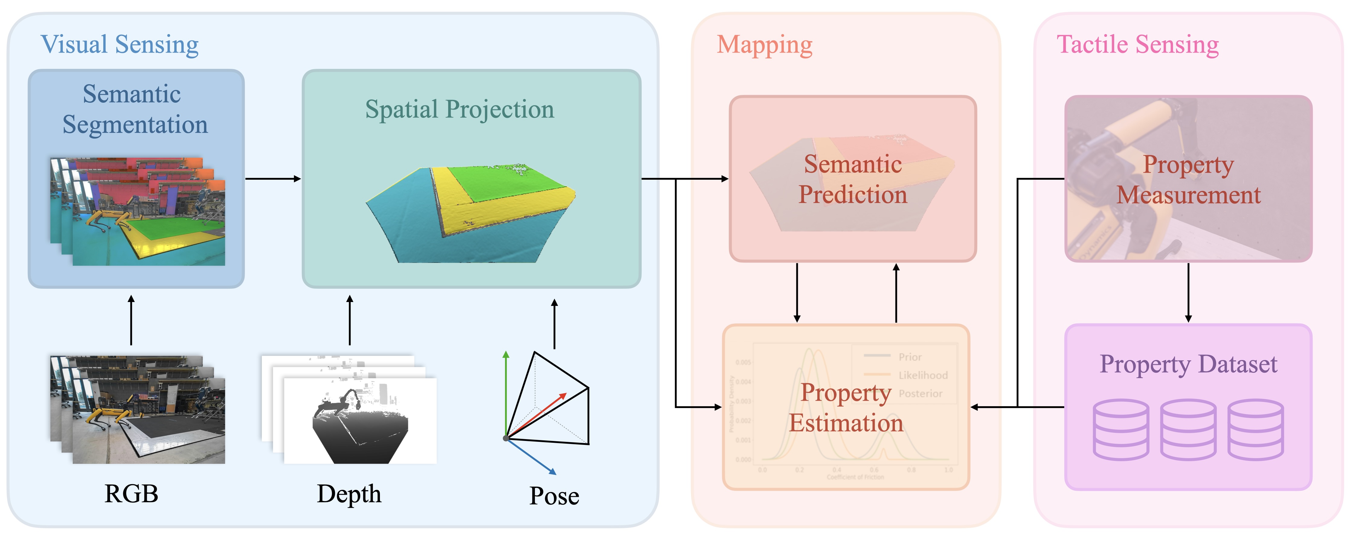
Figure 2: A flow diagram illustrating Algorithm 2. A semantic classification algorithm predicts pixel-wise classes from RGB images that are then projected into a common mapping frame using the aligned depth image, camera intrinsics, and estimated camera pose. This semantic point cloud is used to build a metric-semantic map. When a property measurement is taken, Algorithm 1 is used to update the semantic and property estimates.

IV Algorithm Overview

1 $\mathcal{M}\leftarrow$ initMap()

2 $\Theta\leftarrow$ initUncertainty()

3 while robot is running do

4       $s\leftarrow$ getSemanticPointCloud()

       $\mathcal{M}\leftarrow$ updateMap($s$) // Sec.V

       $\Theta\leftarrow$ updateSemanticUncertainty($s$) // Sec.V

5       if  user requests property measurement taken then

6             $\psi\leftarrow$ getMeasurement()

             $\mathcal{V}\leftarrow$ getMeasurementLocation() // Sec.IX

             $\Theta\leftarrow$ measurementUpdate($\psi,\mathcal{V}$) // Alg.1

7            

8      

Algorithm 2 Semantic and Property Prediction

The proposed algorithm takes as input a stream of RGB-D images and physical property measurements from a tactile sensor and outputs semantic classifications and physical property estimates which are modelled probabilistically. We provide an overview of the proposed method presented in Algorithm 2. We focus on tactile and visual modalities, however our method may be adapted to different sensing modalities in a straight-forward manner.

A metric-semantic map and Dirichlet parameters are first initialized, where $\bm{\alpha}=\bm{1}_{k\times 1}$ (Lines 2 - 2). We assume that, while the robot is running, it is collecting exteroceptive data in the form of RGB-D images or lidar data. Using an off-the-self semantic segmentation network of choice, this data is transformed into a semantic point cloud [36] (Line 2). The geometric information of this point cloud is used to update the metric map (Line 2) while the semantic classifications are used to compute the semantic class posterior (Line 2), as described in Section V.

Locations for property measurements are specified by the user. When a property measurement is taken using a tactile sensor, we first compute the region over which the measurement was taken within the map and use moment matching (Algorithm 1) to update the semantic classifications and property estimates within this region (Lines 2-2). We describe this step in more detail in Section VI. A flow diagram illustrating this procedure is given in Figure 2.

V Vision-Based Estimation

This section describes how to implement Bayesian inference to recursively estimate semantic classifications using visual data. This corresponds to the Visual Sensing block in Figure 2. First, we discuss how to obtain a semantic segmentation point cloud and then discuss how to probabilistically fuse this data within a geometric representation.

Semantic segmentation assigns task-dependent class probability scores to each pixel in an image. It is commonplace to use neural networks to estimate pixel-wise class probability scores [37]. Let $I\in\mathbb{R}^{w\times h\times 3}$ denote an RGB image, where $h,w$ are the height and width of the image in pixels. A trained semantic segmentation network takes an input image $I$ and outputs the pixel-wise class probability scores $T\in\mathbb{R}^{w\times h\times k}$ for $k$ semantic classes in the form of a k-dimensional Categorical distribution. By employing a one-hot encoding over these pixel-wise scores, $H=1\{T\}$ such that $H\in\mathbb{R}^{w\times h}$, we may interpret the network as drawing pixel-wise class samples from pixel-wise Categorical distributions. We denote these as the semantic class measurements, the accuracy of which depends on the network used.

We use an aligned depth image, camera intrinsics, and camera pose estimate to project the semantic class measurements $H$ into a fixed global coordinate frame [36, (10.38)] to obtain a point cloud representation of the semantically segmented image. Akin to [38] we implement a modified version of Kinect Fusion [39], a truncated signed distance field (TSDF), as the geometric representation onto which semantic class measurements are projected. Within each voxel we store unique Dirichlet parameters $\bm{\alpha}$. Given new semantic class measurements, we update these parameters in each voxel using (6). Thus, semantic classification estimates may be recursively obtained with uncertainty estimates via (5).

VI Tactile-Based Estimation

This section describes how semantic class estimates may be used to predict physical properties and how we use measurements of these properties to update semantic class likelihoods. This corresponds to the Tactile Sensing block in Figure 2. Our goal is to compute a measurement likelihood for physical properties using semantic class likelihoods introduced in Section V.

Motivated by [5, 40], we construct a conditional probability distribution $p(\bm{\psi}\mid\mathcal{Z})$ for a property $\psi$ with semantic data $\mathcal{Z}$. By applying the law of total probability and including the $\bm{\alpha}$ parameters introduced in Section III-A1, we derive the following expression:

$$p(\bm{\psi}\mid\mathcal{Z},\bm{\alpha})=\sum_{i=1}^{k}p(\bm{\psi}\mid z=i)p(z=i\mid\mathcal{Z},\bm{\alpha}).$$ (27)

There are two components to this equation. The first, $p(z=i\mid\mathcal{Z},\bm{\alpha})$, is the posterior predictive likelihood of a region of the map belonging to semantic class $i$ given prior semantic class measurements within that region. This posterior predictive likelihood was derived in Section III-A and is given by (9).

Physical properties are not constant across a semantic class and thus should be estimated via a distribution of possible values, not by a single value. The second component, $p(\bm{\psi}\mid z=i)$, denotes this likelihood distribution and is approximated as a Gaussian distribution [5]. Substituting (9) and the formula for the class-wise Gaussian model into (27) gives a closed-form estimate for the physical properties given semantic class measurements:

$$p(\bm{\psi}\mid\mathcal{Z},\bm{\alpha})=\sum_{i=1}^{k}\frac{\alpha_{i}}{\sum_{j=1}^{k}\alpha_{j}}\mathcal{N}(\mu_{i},\sigma_{i}^{2}).$$ (28)

Note that this model is equivalent to the Gaussian mixture model presented in (10) where the weights are computed using the predictive posterior of the semantic classifications. We use this as the measurement likelihood for the properties of interest.

Semantic Class	Gaussian Parameters
	$\mu$	$\sigma$
Concrete	0.543	0.065
Grass	0.577	0.077
Rock	0.478	0.133
Wood	0.372	0.055
Rubber	0.616	0.048
Plastic	0.311	0.045
Snow	0.390	0.071
Ice	0.192	0.046

TABLE I: Gaussian parameters for the coefficient of friction of semantic classes. These values are computed using the material friction dataset provided by [5] and assume rubber as the contact material.

Given that the Gaussian mixture model is used as the measurement likelihood, we use the approximate conjugate prior of this distribution, the Dirichlet Normal-Inverse-Gamma product, to represent uncertainty in the semantic classifications, $w_{i}$, and class-wise property parameters, $\mu_{i}$ and $\sigma^{2}_{i}$. Note that the Gaussian mixture weights, $w_{i}$, are computed using the Dirichlet parameters $\bm{\alpha}$. After a property measurement is taken, Algorithm 1 is implemented to update the belief over these parameters via (21). This algorithm is applied sequentially if multiple measurements are taken.

Using Algorithm 1, the semantic class likelihood, $w_{i}$, as well as the property parameters themselves, $\mu_{i}$ and $\sigma^{2}_{i}$, are updated. Furthermore, the Dirichlet Normal-Inverse-Gamma product posterior provides a means of uncertainty quantification in the posterior estimates of the semantic class likelihoods and property values, unlike learning-based approaches.

VII Implementation

Algorithms 1 and 2 are implemented in C++ and include a ROS interface which will be released upon final submission of the paper. Experiments are conducted on a laptop with a 5.4GHz i9-13900HX processor, 32GB of RAM, and an Nvidia RTX 4060 GPU.

We use a custom implementation of the SegFormer network [41] trained on the Dense Material Segmentation Dataset [12]. The output of the network is then post-processed with a segment-based voting scheme using FastSAM [28] in a similar manner to [42]. When a property measurement is taken, Algorithm 1 updates a region of the geometric representation segmented using FastSAM. This incentivizes regions with spatial proximity and visual similarity to be updated using a single measurement rather than requiring one measurement for each voxel, making the algorithm more efficient.

Table I is used to initialize the Gaussian parameters for the coefficient of friction for the relevant semantic classes. The values in Table I were computed using the material friction dataset provided by [5]. If a friction measurement is taken of a material class not present in Table I, Algorithm 1 predicts the class from Table I with the most similar friction values.

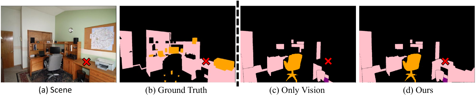
Figure 3: Results for a single simulated experiment. The image (a) and ground truth semantic labels (b) are from the Dense Material Segmentation Dataset [12]. The semantic segmentation predictions (c) do not classify parts of the desk as wood. A friction measurement is simulated using the ground-truth semantic label and Table I and is sampled from the pixel highlighted by the red cross in the RGB image. Algorithm 1 then computes the correct posterior semantic label (d).

For hardware demonstrations, static friction measurements are taken using a force-torque sensor which measures contact forces during the motion of an end-effector against a surface. These forces are converted to friction measurements using the equation relating normal and tangential forces:

$$\psi=\frac{F_{t}}{F_{n}},$$ (29)

where $F_{t}$ is the force tangential to the contact normal, $F_{n}$ is the force parallel to the contact normal, and $\psi$ is the coefficient of friction. A low-pass filter is used to filter out measurement noise from the force-torque sensor.

VIII Simulation Results

We validate our approach in simulation and demonstrate property measurements improve semantic predictions. The simulation experiments also validate the approximation accuracy of the moment matching method in Algorithm 1 in approximating the posterior via Theorem 3.

We use 1800 images and ground-truth semantic labels taken from the testing set of the Dense Material Segmentation Dataset [12] and the pre-trained semantic segmentation neural network described in Section VII is used to predict semantic labels. Misclassified pixels in each image are randomly selected and a friction measurement is drawn from a Gaussian distribution whose parameters are specified in Table I using the corresponding ground-truth semantic label. The semantic prediction is used to initialize the Dirichlet parameters such that $\bm{\alpha}=1_{k\times 1}+1\{z=j\}$. The Gaussian parameters are initialized via Table I and the remaining Dirichlet Normal-Inverse-Gamma parameters are initialized as $\bm{a}=\bm{\alpha}$, and $\tau_{i}=\mu_{i}$, $\kappa_{i}=1$, $\beta_{i}=\sigma_{i}^{2}/\tau_{i}$, $\gamma_{i}=\sqrt{\beta_{i}}/C$, and $C=40$ for each semantic class.

After a simulated friction measurement is randomly sampled, Algorithm 1 is invoked and the posterior predictive likelihood is computed. The Segment Anything Model [42] computes a mask over the input RGB image using the chosen pixel as the query point and the semantic predictions over this region are updated corresponding to the posterior predictive likelihood output by Algorithm 1. An example of this computed posterior is demonstrated in Figure 3.

Semantic Class	mAcc % Increase	Max Acc % Increase
Concrete	$38.6\pm 51.9$	192.8
Grass	$14.2\pm 32.8$	129.8
Rock	$26.4\pm 41.1$	191.2
Wood	$24.5\pm 35.0$	190.0
Rubber	$5.7\pm 12.3$	50.8
Plastic	$13.5\pm 26.6$	184.4
Snow	$0.00\pm 0.00$	0.00
Ice	$110.1\pm 0.0$	110.1
Total	$21.3\pm 34.3$	192.8

TABLE II: Increase in mean pixel-wise semantic prediction accuracy using simulated property measurements and Algorithm 1. Property measurements are shown to improve semantic prediction accuracy for all material classes from Table I except snow. The standard deviation for mean pixel-wise accuracy increase is also shown in the second column. The third column shows the maximum increase in pixel-wise semantic prediction accuracy seen in the simulation experiments.

The mean pixel-wise accuracy of the semantic segmentation network over this dataset without applying the proposed algorithm is 27.2%. The mean pixel accuracy of the posterior semantic predictions output by Algorithm 1 is 33.0%, an increase of 21.3%, demonstrating increased semantic prediction performance compared to semantic predictions using vision alone.

Table II provides a further breakdown of the increase in the pixel-wise semantic prediction accuracy for each material class. Notably, materials such as rock, plastic, and concrete occupy the majority of pixels in some images, which leads to increases in pixel-wise accuracy of over 75%. All classes except for snow saw improved semantic prediction performance using simulated tactile sensing. When simulating tactile measurements for snow, Algorithm 1 incorrectly predicts the semantic class as either rock or wood because the Gaussian parameters for snow are similar to those of these two classes. Interestingly, depending on the simulated friction measurement, the Gaussian mixture mode responsible for predicting snow collapses and the mode for either rock or wood becomes dominant. Only one image in the Dense Material Segmentation Dataset test set contained ice.

This experiment highlights that by conditioning semantic classifications on physical properties, one can generally improve the accuracy of visual semantic classifications.

IX Hardware Experiments

Next, we validate our method on several hardware demonstrations and compare against existing semantic mapping and property estimation approaches. In the first demonstration, we validate the results from simulation and show that our approach is capable of correcting erroneous semantic classifications by measuring the coefficient of friction. We then provide two case studies for the utility of estimating physical properties. For the first case study, our proposed approach is used within a risk-aware legged locomotion planner to update the locomotion gait of a quadruped when hazardous terrain is perceived. In the second case study, we demonstrate our approach is able to estimate affordance-based properties in a door-opening scenario. Both case studies are presented on the accompanying project webpage.

IX-A Semantic Prediction Using Property Measurements

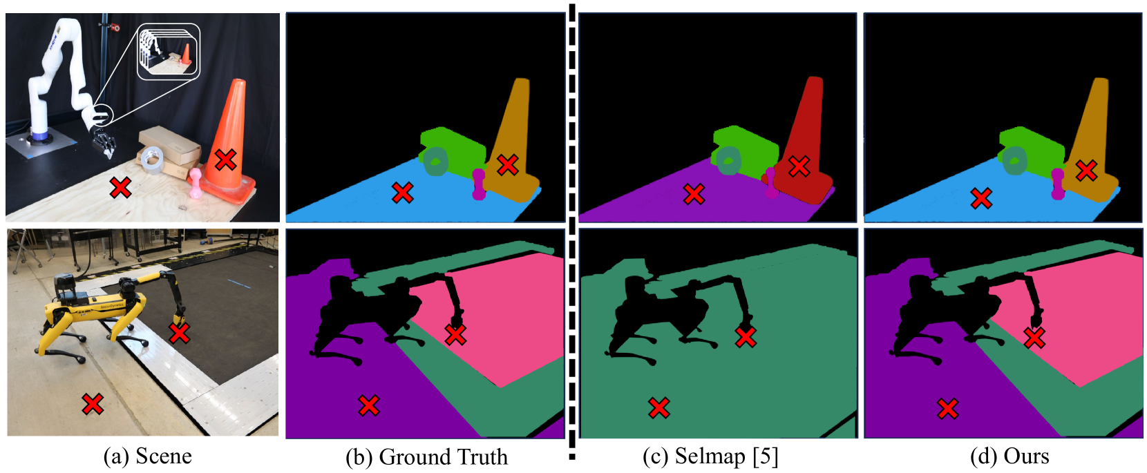
Figure 4: A semantic segmentation task is shown and the proposed method is compared against the semantic mapping approach from [5] which is called Selmap. The expected semantic class is shown. a) The input image with measurement locations shown using an X and associated b) ground truth semantic labels are provided. Both Selmap and our approach use the same SegFormer + FastSAM pre-trained semantic segmentation network specified in Section VII. This network incorrectly predicts the semantic labels for several regions within the scene. c) This incorrect labelling is reflected in the Selmap implementation as the visual-based semantic mapping approach is unable to correct these erroneous predictions. By exploiting a tactile sensing modality, d) our approach is able to correct the erroneous semantic predictions and correctly predict the semantic labels of the objects within the scene.

The end-effector of a Kinova Gen 3 robotic arm and a Spot Arm are used to collect friction measurements using built-in wrist-mounted force-torque sensors. For this experiment, 5 frames from the RGB-D stream are used to initialize the semantic TSDF map. Each RGB-D image is semantically segmented using the trained network and projected into the global coordinate frame using the aligned depth image. The recursive vision-based semantic update described in Section V is applied for each semantic point cloud. This initializes the $\bm{\alpha}$ parameters in (28) used to compute the initial semantic classification weights for the measurement likelihood. The Gaussian parameters are initialized via Table I and the remaining Dirichlet Normal-Inverse-Gamma parameters are initialized as per Section VIII.

We compare our approach to the recursive semantic mapping approach of [5] which only uses vision. The same SegFormer-FastSAM semantic segmentation network is used for both methods. As shown in Figure 4, the network incorrectly classifies various objects in the scenes. When only vision-based semantic classifications are considered [5], the erroneous predictions from the network are unable to be corrected (Figure 4c).

Using the proposed method, a user specifies the location for friction measurements to be taken (Figure 4a). Algorithm 1 then computes the posterior semantic classification weights using the friction measurements as input. This corrects the expected semantic classification, as shown in Figure 4d.

We ran the experiment on two indoor scenes with two friction measurements each as depicted in Figure 4. As shown in Figure 4, the semantic prediction accuracy increases using the proposed method and matches the ground-truth semantic labels. In contrast, [5] is unable to correct the erroneous predictions from the semantic segmentation network, resulting in incorrect semantic predictions. This demonstrates that the simulation results shown in Section VIII translate to hardware experiments.

IX-B Friction Estimation Using Semantics

We demonstrate the utility of our proposed property estimation method using a case study involving a challenging legged locomotion traversal task of crossing an icy surface. We implement a locomotion planner similar to [43] that switches between predetermined static and dynamic gaits depending on the expected value for the coefficient of friction of the terrain to be traversed. A static gait is used when the expected value for the coefficient of friction falls below a threshold of $\mathbb{E}[\psi]\leq 0.25$.

A stream of RGB-D images is used to build a semantic TSDF map of the robot’s environment as outlined in Section V. The resultant semantic TSDF map predicts that the region the robot must traverse may have a low coefficient of friction and a measurement is therefore taken to better approximate the value.

The Dirichlet Normal-Inverse-Gamma prior parameters are initialized as described in Section VIII. We use the manipulator mounted to the legged robot to take friction measurements of the ground in front of the robot using a built-in wrist-mounted force-torque sensor via (29). Algorithm 1 then computes the posterior estimate for the coefficient of friction (Figure 1).

The experiment was conducted six times in the same location during the same afternoon, three where the robot does not measure the coefficient of friction and three where it does. The prior and posterior friction estimates for these six trials is shown in Figure 5. The semantic segmentation network incorrectly predicts the semantic label of the terrain for each run and mis-classifies the ice as either concrete or snow. Since a friction measurement is not taken, the friction threshold $\mathbb{E}[\psi]\leq 0.25$ is not met due to mislabeling and the robot attempts to cross the ice using a dynamic gait, resulting in it slipping and falling for all three of these trials.

For the subsequent two trials, friction measurements of $\psi_{1}=0.139$ and $\psi_{2}=0.156$ are taken for each trial, respectively. After computing the posterior friction estimates via Algorithm 1, the friction threshold is met and the robot switches to a static, stable gait to cross the ice. This results in successful ice traversal for these two trials. In the following third trial, a friction measurement of $\psi_{3}=0.628$ is taken due to erroneous end-effector placement. The computed posterior is shown in Figure 5 and shows a coefficient of friction with a large expected value which exceeds the threshold. For this trial, the robot remains in a dynamic gait and slips on the ice during traversal. A video of a successful ice traversal trial is provided on the accompanyig project webpage.

We further compare our property estimation approach with two state-of-the-art traversability estimation methods designed for legged locomotion. Both methods consider both geometric and semantic features and use a pre-trained neural network to estimate a traversability score [44, 3]. Both traversability estimation methods predict that the icy surface is traversable as shown in Figure 6; however, attempting to traverse this surface using a dynamic gait resulted in the robot slipping and falling.

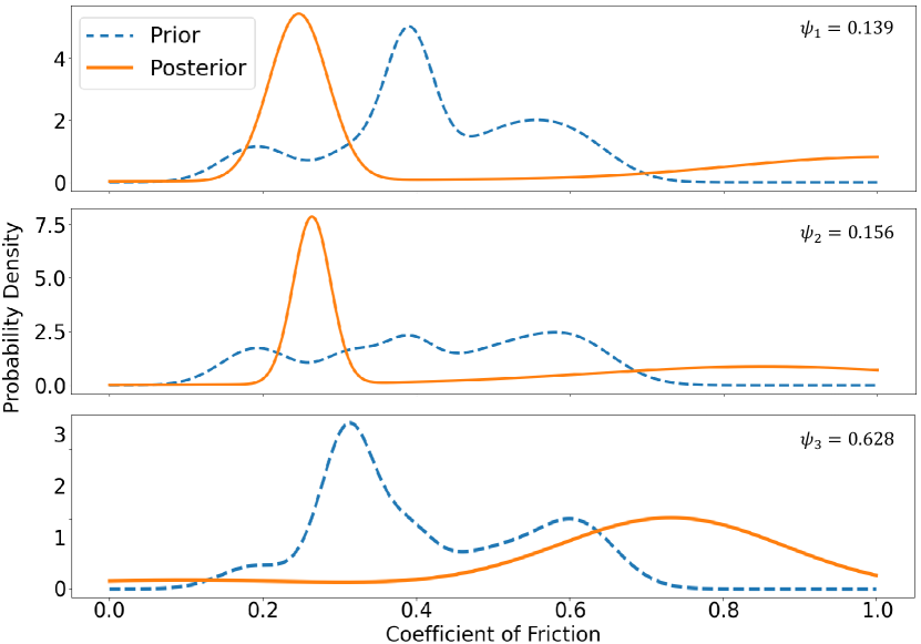
Figure 5: The prior (dotted) and posterior (solid) friction estimates for the three ice traversal demonstration runs. When friction measurements are taken of the ice before traversal, Algorithm 1 predicts the posterior friction estimates. The friction measurements are $\psi_{1}=0.139$, $\psi_{2}=0.156$, and $\psi_{3}=0.628$ for trials 1, 2, and 3, respectively.

Our proposed method is able to verify the property predictions estimated using visual information via tactile sensing and Bayesian inference whereas other state-of-the-art property estimation methods are unable to incorporate multiple sensing modalities. This task highlights the utility of estimating physical properties such as the coefficient of friction to accomplish challenging tasks such as legged locomotion traversal across an icy surface. State-of-the-art traversability estimation methods depend only on the terrain geometry and classification and thus do not provide the means by which a robot may adapt its traversal strategy to account for the properties (i.e. friction) which dictate traversability.

IX-C Encoding Affordance-Based Properties

Lastly, we present a scenario in which our approach is used to estimate affordance-based properties. An affordance is a property of an object that defines its possible used [45]. In this case, we focus on the affordance of a door handle, which affords either a push or pull action, as the semantic classification and examine the force required to open the door as the property of interest.

As shown in Figure 7, a mobile manipulator is used to measure the force required to open a door. Negative forces constitute pushing while positive forces constitute pulling. We equally weight each push/pull affordance and initialize a mean force magnitude of $20N$ and a variance of $10N$.

To measure the force required to open the door, the robot begins applying a pulling force $10N$ and ramps this up to $70N$ over a period of 3 seconds. At $57N$ the door begins to open and this value is used as the property measurement for Algorithm 1. The door opening force posterior is show in Figure 7 in the lower right-hand corner. After invoking Algorithm 1 the push/pull affordances are still almost equally weighed. Additionally, the variance for the pulling force mode has increased, mirroring the fact that a higher-than-expected force was required to open the door. This door opening experiment is demonstrated on the accompanying project webpage.

Next, we test the force required to open six different doors, three pull-to-open and three push-to-open, and use Algorithm 1 to compute the posterior door opening force estimate sequentially after each trail. Figure 8 shows the prior and posterior opening force estimate after each trial. After six trials the estimated door opening force posterior has maintained two modes corresponding to the push or pull force modalities, however the variance has increased, representing the varied door opening forces seen in the experiments compared to the initial estimate.

This case study demonstrates the utility of the proposed method for affordance-based property estimation and opens an avenue for future research given recent advances in affordance-based planning [46].

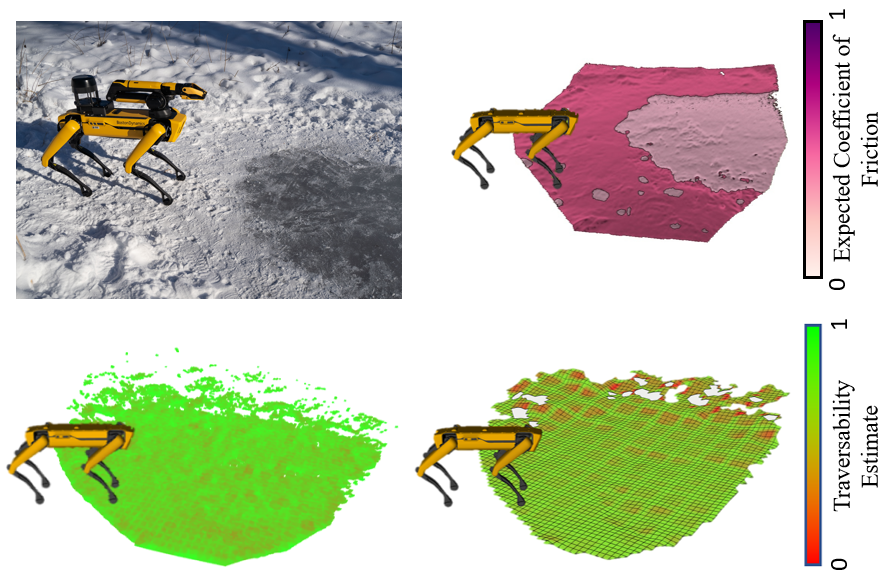
Figure 6: The performance of the proposed approach after a friction measurement is taken in comparison to the traversability estimate computed by [44] (bottom left) and [3] (bottom right). The proposed method is able to correctly predict that the surface in front of the robot has a low coefficient of friction which informs the locomotion planner to switch to a stable gait. In contrast, the traversability estimates predict the ice is traversable even when the robot is using a dynamic gait, which results in the robot slipping and falling.

X Discussion and Conclusion

We propose a method for jointly estimating semantic labels and physical properties. We model semantic classifications and physical properties probabilistically enabling closed-form Bayesian inference given visual semantic predictions and tactile property measurements. We demonstrate that by leveraging this probabilistic approach we are able to improve semantic prediction accuracy by an average of $21.3\%$ in simulation. Additionally, we provide two case studies which motivate the utility of physical property estimation demonstrated in the proposed method.

One drawback of our approach is that the accuracy of our method is reliant on the accuracy of the semantic classification network. If a semantic classification network consistently predicts incorrect semantic labels over a long duration, the initial Dirichlet parameters will skew heavily towards the incorrect semantic label and be difficult to correct with property measurements. Additionally, like many voxel-based semantic mapping frameworks, our method is constrained by memory limitations which restrict the size of the map. We aim to address these concerns in future work. Tactile and visual sensing modalities were used for the proposed method, however additional sensing modalities may also be used in place of or in addition to tactile sensing. This is an avenue for future work. Lastly, our presented method provides a link between visual and tactile sensing modalities through physical property estimates and future work will aim to exploit this relationship for active learning.

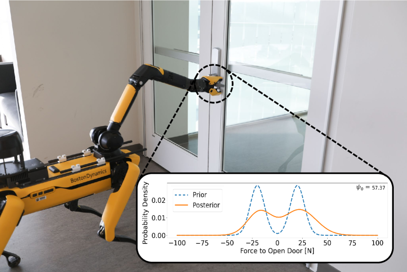
Figure 7: The proposed method is capable of encoding affordance-based properties, in this case the force required to open a door. This door opening force is initialized as a multi-modal distribution with pushing and pulling being equally likely with a magnitude of 20N. The robot applies a pulling force of 57N on the door, resulting in it swinging open. The posterior estimate for the force required to open a door is computed and shown in the embedded plot.

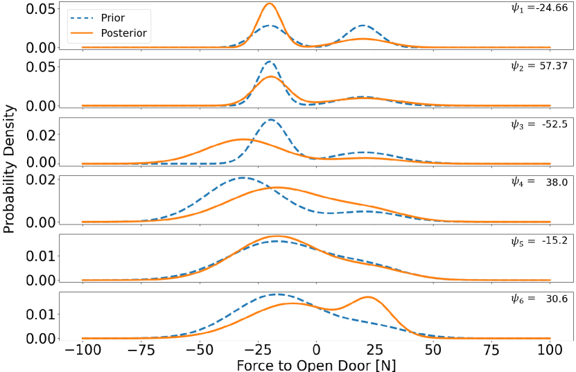
Figure 8: The prior and posterior door opening force estimates running Algorithm 1 sequentially with six experiments, meaning the posterior for the previous experiment is the prior for the current experiment. The force required to open the door is indicated in the upper right-hand corner for each experiment. After measuring the force required to open 6 doors, the posterior estimate has a high variance with an expected value near $0N$, reflecting the equal likelihood that a door is either push or pull to open.

Appendix A Proof of Theorem 1

Let $p(\bm{\theta}|\bm{\alpha})$ be the prior belonging to the family of Dirichlet distributions and $p(z|\bm{\theta})$ the likelihood belonging to the family of Categorical distributions. Let $\mathcal{Z}=\{z_{1},\dots,z_{n}\}$ be a set of measurements drawn from the Categorical likelihood.

The Law of Total Probability is used to compute the posterior distribution:

$$p(\bm{\theta}|\mathcal{Z},\bm{\alpha}) \propto p(\bm{\theta},\mathcal{Z},\bm{\alpha})$$ (30)

$$=p(\bm{\theta}|\bm{\alpha})\prod_{z_{i}\in\mathcal{Z}}p(z_{i}|\bm{\theta}),$$ (31)

where the equality is due to conditional independence.

Then, substituting (1) and (2) into (31), we arrive at:

$$p(\bm{\theta}|\bm{\alpha})\prod_{z_{i}\in\mathcal{Z}}p(z_{i}|\bm{\theta}) \propto\prod_{j=1}^{k}\theta_{j}^{\alpha_{j}-1}\prod_{z_{i}\in\mathcal{Z}}\prod_{j=1}^{k}\theta_{j}^{1\{z_{i}=j\}}$$ (32)

$$=\prod_{j=1}^{k}\theta_{j}^{\alpha_{j}-1+\sum_{z_{i}\in\mathcal{Z}}1\{z_{i}=j\}}.$$ (33)

This is exactly the Dirichlet distribution with parameters

$$\tilde{\alpha}_{j}=\alpha_{j}+\sum_{z_{i}\in\mathcal{Z}}1\{z_{i}=j\}.$$ (34)

Appendix B Proof of Theorem 3

Let $p(\Theta|\Psi)$ be the prior belonging to the family of Dirichlet Normal-Inverse-Gamma distributions and $p(\psi|\Theta)$ the likelihood belonging to the family of Gaussian mixtures. Let $\psi$ be a measurements drawn from the Gaussian mixture likelihood.

From Theorem 2, the posterior of $\Theta$ is given by:

$$p(\Theta|\psi,\Psi)=\frac{1}{M}\sum_{j=1}^{k} c_{j}Dir(\bm{w}|\tilde{\bm{a}}_{j})\cdot$$

$$\cdot\mathcal{NIG}(\mu_{j},\sigma^{2}_{j}|\tilde{\tau}_{j},\tilde{\kappa}_{j},\tilde{\beta}_{j},\tilde{\gamma}_{j})\cdot$$

$$\cdot\prod_{i\neq j}^{k}\mathcal{NIG}(\mu_{i},\sigma^{2}_{i}|\tau_{i},\kappa_{i},\beta_{i},\gamma_{i}),$$ (35)

with parameters computed as per (14)-(19).

It is evident that the number of terms in this posterior grows exponentially for each measurement. To overcome this challenge, we project (B) onto the family of Dirichlet Normal-Inverse-Gamma product distributions using the method of moments. We now prove the set of sufficient moments for the Dirichlet Normal-Inverse-Gamma product distribution is $\mathbb{S}=\{\mu_{i},\sigma^{2}_{i},\sigma_{i}^{4},\mu_{i}^{2}\sigma^{2}_{i},w_{i},w_{i}^{2}\}_{i=1}^{k}$.

From (21), it is evident that $\bm{w}$ drawn from the Dirichlet distribution and $\Phi_{i}=\{\mu_{i},\sigma_{i}\}$ drawn from the Normal-Inverse-Gamma distributions are independent random variables. Therefore, to find the sufficient moments of the Dirichlet Normal-Inverse-Gamma product distribution, we may use the sufficient moments for the Dirichlet and Normal-Inverse-Gamma distributions. The sufficient moments for the Dirichlet distribution are $\{\bm{w},\bm{w}^{2}\}$ [47] and the sufficient moments of the $i$-th Normal-Inverse-Gamma distribution are $\{\mu_{i},\sigma^{2}_{i},\sigma_{i}^{4},\mu_{i}^{2}\sigma^{2}_{i}\}$ [48, Chapter 4.5]. The concatenation of these sufficient moments then constitute the sufficient moments of (21).

The parameters of the Dirichlet Normal-Inverse-Gamma product distribution are then computed via (14)-(19) using the sufficient statistics as derived in [47] and [48], respectively.

B-A Computing the Sufficient Statistics

The sufficient statistics $\mathbb{S}=\{\mu_{i},\sigma^{2}_{i},\sigma_{i}^{4},\mu_{i}^{2}\sigma^{2}_{i},w_{i},w_{i}^{2}\}_{i=1}^{k}$ for (21) must be computed from (B). It is possible to use numerical integration to compute the sufficient moments via (20), however we demonstrate a more computationally efficient method here by exploiting the linearity of the expectation operator and the independence of variables within (B).

We derive the first sufficient moment $\mathbb{E}[\mu_{i}]$ and leave the remaining moment derivations to the reader. We start by noting the independence of $\bm{w}$ and each set of parameters $\Phi_{i}=\{\mu_{i},\sigma^{2}_{i}\}$. Thus, to compute $\mathbb{E}[\mu_{i}]$, we begin by marginalizing out all independent variables from (B), resulting in:

$$\mathbb{E}[\mu_{i}] =\int_{\mu_{i}}\frac{\mu_{i}}{M}\Big{[}c_{i}\mathcal{NIG}(\mu_{i},\sigma^{2}_{i}|\tilde{\tau}_{i},\tilde{\kappa}_{i},\tilde{\beta}_{i},\tilde{\gamma}_{i})+$$

$$\;\;\;\;\;+\sum_{j\neq i}^{k}c_{j}\mathcal{NIG}(\mu_{i},\sigma^{2}_{i}|\tau_{i},\kappa_{i},\beta_{i},\gamma_{i})\Big{]}\mathrm{d}\mu_{i}$$ (36)

$$=\frac{1}{M}\Big{[}c_{i}\int_{\mu_{i}}\mu_{i}\mathcal{NIG}(\mu_{i},\sigma^{2}_{i}|\tilde{\tau}_{i},\tilde{\kappa}_{i},\tilde{\beta}_{i},\tilde{\gamma}_{i})\mathrm{d}\mu_{i}+$$

$$\;\;\;\;\;+\sum_{j\neq i}^{k}c_{j}\int_{\mu_{i}}\mu_{i}\mathcal{NIG}(\mu_{i},\sigma^{2}_{i}|\tau_{i},\kappa_{i},\beta_{i},\gamma_{i})\mathrm{d}\mu_{i}\Big{]}$$ (37)

$$=\frac{1}{M}\Big{[}c_{i}\tilde{\tau_{i}}+\sum_{j\neq i}^{k}c_{j}\tau_{i}\Big{]}$$ (38)

where the first equality follows from the linearity of the expectation operator and the second equality follows from the the fact that for a Normal-Inverse-Gamma distribution, $\mathcal{NIG}(\mu,\sigma^{2}|\tau,\kappa,\beta,\gamma)$, the expected value for $\mu$ is simply $\mathbb{E}[\mu]=\tau$.

References

- [1] Yanming Guo, Yu Liu, Theodoros Georgiou and Michael S Lew “A review of semantic segmentation using deep neural networks” In International journal of multimedia information retrieval 7 Springer, 2018, pp. 87–93
- [2] Ashish Vaswani et al. “Attention is all you need” In Advances in neural information processing systems 30, 2017
- [3] Lu Gan et al. “Multitask learning for scalable and dense multilayer bayesian map inference” In IEEE Transactions on Robotics 39.1 IEEE, 2022, pp. 699–717
- [4] John McCormac, Ankur Handa, Andrew Davison and Stefan Leutenegger “Semanticfusion: Dense 3d semantic mapping with convolutional neural networks” In 2017 IEEE International Conference on Robotics and automation (ICRA), 2017, pp. 4628–4635 IEEE
- [5] Parker Ewen et al. “These Maps are Made for Walking: Real-Time Terrain Property Estimation for Mobile Robots” In IEEE Robotics and Automation Letters 7.3 IEEE, 2022, pp. 7083–7090
- [6] Xiaoyi Cai et al. “EVORA: Deep Evidential Traversability Learning for Risk-Aware Off-Road Autonomy” In arXiv preprint arXiv:2311.06234, 2023
- [7] Shijie Hao, Yuan Zhou and Yanrong Guo “A brief survey on semantic segmentation with deep learning” In Neurocomputing 406 Elsevier, 2020, pp. 302–321
- [8] Robin Strudel, Ricardo Garcia, Ivan Laptev and Cordelia Schmid “Segmenter: Transformer for semantic segmentation” In Proceedings of the IEEE/CVF international conference on computer vision, 2021, pp. 7262–7272
- [9] Jia Deng et al. “Imagenet: A large-scale hierarchical image database” In 2009 IEEE conference on computer vision and pattern recognition, 2009, pp. 248–255 Ieee
- [10] Tsung-Yi Lin et al. “Microsoft coco: Common objects in context” In Computer Vision–ECCV 2014: 13th European Conference, Zurich, Switzerland, September 6-12, 2014, Proceedings, Part V 13, 2014, pp. 740–755 Springer
- [11] Benjamin Kuipers and Yung-Tai Byun “A robot exploration and mapping strategy based on a semantic hierarchy of spatial representations” In Robotics and autonomous systems 8.1-2 Elsevier, 1991, pp. 47–63
- [12] Paul Upchurch* and Ransen Niu* “A Dense Material Segmentation Dataset for Indoor and Outdoor Scene Parsing” In ECCV, 2022 URL: https://arxiv.org/abs/2207.10614
- [13] Ioannis Kostavelis and Antonios Gasteratos “Semantic mapping for mobile robotics tasks: A survey” In Robotics and Autonomous Systems 66 Elsevier, 2015, pp. 86–103
- [14] Niko Sünderhauf et al. “Meaningful maps with object-oriented semantic mapping” In 2017 IEEE/RSJ International Conference on Intelligent Robots and Systems (IROS), 2017, pp. 5079–5085 IEEE
- [15] Joey Wilson et al. “ConvBKI: Real-Time Probabilistic Semantic Mapping Network with Quantifiable Uncertainty” In arXiv preprint arXiv:2310.16020, 2023
- [16] Camille Couprie, Clément Farabet, Laurent Najman and Yann LeCun “Indoor semantic segmentation using depth information” In arXiv preprint arXiv:1301.3572, 2013
- [17] Peng Wang et al. “Towards unified depth and semantic prediction from a single image” In Proceedings of the IEEE conference on computer vision and pattern recognition, 2015, pp. 2800–2809
- [18] Yuxiang Sun et al. “FuseSeg: Semantic segmentation of urban scenes based on RGB and thermal data fusion” In IEEE Transactions on Automation Science and Engineering 18.3 IEEE, 2020, pp. 1000–1011
- [19] Nathan Silberman, Derek Hoiem, Pushmeet Kohli and Rob Fergus “Indoor segmentation and support inference from rgbd images” In Computer Vision–ECCV 2012: 12th European Conference on Computer Vision, Florence, Italy, October 7-13, 2012, Proceedings, Part V 12, 2012, pp. 746–760 Springer
- [20] Dong-Ki Kim, Daniel Maturana, Masashi Uenoyama and Sebastian Scherer “Season-invariant semantic segmentation with a deep multimodal network” In Field and Service Robotics: Results of the 11th International Conference, 2018 Springer
- [21] Abhinav Valada, Rohit Mohan and Wolfram Burgard “Self-supervised model adaptation for multimodal semantic segmentation” In International Journal of Computer Vision 128.5 Springer, 2020
- [22] Martim Brandao, Kenji Hashimoto and Atsuo Takanishi “Friction from vision: A study of algorithmic and human performance with consequences for robot perception and teleoperation” In 2016 IEEE-RAS 16th International Conference on Humanoid Robots (Humanoids), 2016, pp. 428–435 IEEE
- [23] Donghun Noh et al. “Surface material dataset for robotics applications (SMDRA): A dataset with friction coefficient and RGB-D for surface segmentation” In 2020 25th International Conference on Pattern Recognition (ICPR), 2021, pp. 6275–6281 IEEE
- [24] Shifeng Wang “Road terrain classification technology for autonomous vehicle” Springer, 2019
- [25] Panagiotis Papadakis “Terrain traversability analysis methods for unmanned ground vehicles: A survey” In Engineering Applications of Artificial Intelligence 26.4 Elsevier, 2013, pp. 1373–1385
- [26] Jonas Frey, David Hoeller, Shehryar Khattak and Marco Hutter “Locomotion policy guided traversability learning using volumetric representations of complex environments” In 2022 IEEE/RSJ International Conference on Intelligent Robots and Systems (IROS), 2022, pp. 5722–5729 IEEE
- [27] Dongshin Kim et al. “Traversability classification using unsupervised on-line visual learning for outdoor robot navigation” In Proceedings 2006 IEEE International Conference on Robotics and Automation, 2006. ICRA 2006., 2006, pp. 518–525 IEEE
- [28] Jonas Frey et al. “Fast Traversability Estimation for Wild Visual Navigation” In arXiv preprint arXiv:2305.08510, 2023
- [29] Carmelo Sferrazza et al. “The Power of the Senses: Generalizable Manipulation from Vision and Touch through Masked Multimodal Learning” In arXiv preprint arXiv:2311.00924, 2023
- [30] Gabriel B Margolis, Xiang Fu, Yandong Ji and Pulkit Agrawal “Learning to See Physical Properties with Active Sensing Motor Policies” In arXiv preprint arXiv:2311.01405, 2023
- [31] Sebastian Thrun “Probabilistic robotics” In Communications of the ACM 45.3 ACM New York, NY, USA, 2002, pp. 52–57
- [32] Persi Diaconis and Donald Ylvisaker “Conjugate priors for exponential families” In The Annals of statistics JSTOR, 1979, pp. 269–281
- [33] Brian DO Anderson and John B Moore “Optimal filtering” Courier Corporation, 2012
- [34] Stephen Tu “The dirichlet-multinomial and dirichlet-categorical models for bayesian inference” In Computer Science Division, UC Berkeley 2, 2014
- [35] Priyank Jaini and Pascal Poupart “Online and distributed learning of Gaussian mixture models by Bayesian moment matching” In arXiv preprint arXiv:1609.05881, 2016
- [36] Mark S. Nixon and Alberto S. Aguado “Feature Extraction & Image Processing for Computer Vision (Third edition)” In Feature Extraction & Image Processing for Computer Vision (Third Edition) Oxford: Academic Press, 2012, pp. 489–518
- [37] Alberto Garcia-Garcia et al. “A survey on deep learning techniques for image and video semantic segmentation” In Applied Soft Computing 70 Elsevier, 2018, pp. 41–65
- [38] Yu Xiang and Dieter Fox “DA-RNN: Semantic mapping with data associated recurrent neural networks” In arXiv preprint arXiv:1703.03098, 2017
- [39] Shahram Izadi et al. “Kinectfusion: real-time 3d reconstruction and interaction using a moving depth camera” In Proceedings of the 24th annual ACM symposium on User interface software and technology, 2011, pp. 559–568
- [40] Tran Nguyen, Francesco Verdoja, Fares Abu-Dakka and Ville Kyrki “Probabilistic Surface Friction Estimation Based on Visual and Haptic Measurements” In IEEE Robotics and Automation Letters PP, 2021, pp. 1–1
- [41] Enze Xie et al. “SegFormer: Simple and efficient design for semantic segmentation with transformers” In Advances in Neural Information Processing Systems 34, 2021, pp. 12077–12090
- [42] Jiaqi Chen, Zeyu Yang and Li Zhang “Semantic Segment Anything”, https://github.com/fudan-zvg/Semantic-Segment-Anything, 2023
- [43] Paul Filitchkin and Katie Byl “Feature-based terrain classification for littledog” In 2012 IEEE/RSJ International Conference on Intelligent Robots and Systems, 2012, pp. 1387–1392 IEEE
- [44] Ruslan Agishev, Tomáš Petříček and Karel Zimmermann “Trajectory Optimization Using Learned Robot-Terrain Interaction Model in Exploration of Large Subterranean Environments” In IEEE Robotics and Automation Letters 7.2, 2022, pp. 3365–3371 DOI: 10.1109/LRA.2022.3147332
- [45] James J Gibson “The theory of affordances” In Hilldale, USA 1.2, 1977
- [46] Safoura Rezapour Lakani, Antonio J Rodríguez-Sánchez and Justus Piater “Towards affordance detection for robot manipulation using affordance for parts and parts for affordance” In Autonomous Robots 43 Springer, 2019, pp. 1155–1172
- [47] Thomas Minka “Estimating a Dirichlet distribution” Technical report, MIT, 2000
- [48] José M Bernardo and Adrian FM Smith “Bayesian theory” John Wiley & Sons, 2009