Two-index SU(N) theories
 
QCD, Orientifolds, Super Yang-Mills, Lattice
and
Steven Weinberg’s $\displaystyle\pi\pi$ scattering legacy

Abstract

I review and improve on how two-index SU(N) gauge-fermion theories help access salient information about the large $\displaystyle N$ vacuum and spectrum of QCD, super Yang Mills and meson-meson scattering. The interplay with recent lattice simulations will be employed to deduce the size of $\displaystyle 1/N^{2}$ corrections. Through the meson-meson scattering analysis I will honor Steven Weinberg’s memory by showing how two-index extrapolations naturally accommodate the appearance of tetraquarks states crucial to unitarize meson-meson scattering at low energies.

1 Prologue

Steven Weinberg, a titan of physics, profoundly impacted our understanding of the fundamental forces of Nature. His monumental contribution spans from particle physics to cosmology. Weinberg’s work not only advanced the frontiers of theoretical physics but also inspired generations of scientists. His legacy will continue to influence our understanding of the building blocks of nature and the scientific community at large for the time to come. It is hard not to be both amazed and intimidated by Weinberg’s work, always written with such a rigor and clarity but at the same time pragmatic and to the point. Weinberg’s defining work Weinberg:1967tq alongside Glashow and Salam, is the discovery of the electroweak theory, a model blessed by Nature Aad:2012tfa . My past and present research work, like the one of several colleagues, has drawn inspiration by many of Weinberg’s papers from his pioneering work on spontaneous symmetry breaking Goldstone:1961eq to $\displaystyle\pi\pi$ scattering Weinberg:1966kf , effective lagrangians Weinberg:1978kz , dynamical Weinberg:1975gm and radiative Gildener:1976ih symmetry breaking Weinberg:1975gm , high temperature symmetry non restoration Weinberg:1974hy , etc. Rather than even attempting the impossible, for me, task to provide a comprehensive review of Weinberg’s immense body of work I will discuss one of his late research papers about "Tetraquarks mesons in large-$\displaystyle N$ Quantum Chromodynamics" Weinberg:2013cfa and show how to address his main conclusions efficiently and elegantly using an alternative large number of colors limit. I will also review and improve upon the use of the alternative framework to determine spectral properties of QCD, and more generally of $\displaystyle SU(N)$ gauge theories with two-index matter, of immediate relevance for present and future lattice simulations and model building.

Despite the work of physicists of the caliber of Weinberg, strongly coupled dynamics continues to challenge our understanding of nature. It is for this reason that several methodologies have been devised to tackle different corners of strongly coupled quantum field theories from effective approaches Weinberg:1978kz ; Gasser:1984gg ; Gasser:1987ah to large number of colors expansions tHooft:1973alw ; Witten:1980sp ; Corrigan:1979xf ; Coleman_1985 . These methodologies are often fused to increase their impact. A renown example is the ’t Hooft  tHooft:1973alw ; Witten:1980sp large number of colors limit. Here one can explain several properties of QCD with several caveats. For, example, since quark loops are suppressed at large $\displaystyle N$ the properties of the $\displaystyle\eta^{\prime}$-meson are not properly captured. The latter acquires mass via the quantum axial anomaly which is suppressed in ’t Hooft large $\displaystyle N$ limit. Additionally, Coleman in his Erice lectures Coleman_1985 argued that QCD, in the ’t Hooft extrapolation, does not feature tetraquark mesons, i.e. exotic mesons made by a pair of quarks and antiquarks. However, these states do play a crucial role in unitarizing pion pion scattering as I had shown during my PhD work Sannino:1995ik ; Harada:1995dc and, furthermore, Jaffe Jaffe:1976ig had already introduced them to group-theoretically accommodate the low energy scalar spectrum. Tetraquark states have been discussed later in Close:2002zu ; Braaten:2003he ; Pelaez:2003dy ; Close:2003sg ; Maiani:2004uc ; Bignamini:2009sk ; Ali:2011ug ; Achasov:2012kk .

The alternative large $\displaystyle N$ limit was pioneered by Corrigan and Ramond (CR) Corrigan:1979xf soon after ’t Hooft seminal work, introducing quarks transforming according to the two-index antisymmetric representation of the gauge group. By construction the two type of QCD extensions coincide for $\displaystyle N=3$ but differ at large $\displaystyle N$. The CR expansion was introduced to amend the ’t Hooft overzealous suppression of quark loops as $\displaystyle N$ approaches infinity. The CR large $\displaystyle N$ rules and physical applications for scattering amplitudes were investigated in Kiritsis:1989ge ; Sannino:2007yp . As I shall show later these rules elucidate a number of physical properties of the QCD spectrum such as the nature of the lowest lying composite scalar known as $\displaystyle f_{0}(500)$ as a tetraquark state Sannino:2007yp . Besides the ’t Hooft and CR vector-like extrapolations of QCD, a chiral extension was discovered in Ryttov:2005na . In the chiral extension one splits the two Weyl fermions constituting a QCD quark and assigns one Weyl to the fundamental representation and the other to the two-index antisymmetric representation of the gauge group. This theory is chiral for any $\displaystyle N$ larger than three and maps into the generalized Georgi-Glashow model PhysRevLett.32.438 with one vector like fermion. Differently from the ’t Hooft and the CR limits in which the idea is to capture different aspects of QCD, the motivation for a chiral extension is to learn more about the non-perturbative dynamics of the chiral theory itself. In fact, to date lattice simulations of chiral theories are still challenging Kaplan:2023pxd ; Kaplan:2023pvd . In Ryttov:2005na we learnt that there is a non-perturbative phase of the chiral extension where the dynamical formation of a bilinear condensate breaks the gauge symmetry spontaneously and Higgses the theory to ordinary massless one-flavor QCD. The remaining infrared chiral matter is massless and sterile with respect to QCD. The example hints at the possibility that the non-trivial dynamics for chiral gauge theories is vector-like while the residual infrared chiral dynamics is trivial. The distinct large $\displaystyle N$ extensions of QCD are summarised in figure 1 including their salient large $\displaystyle N$ properties.

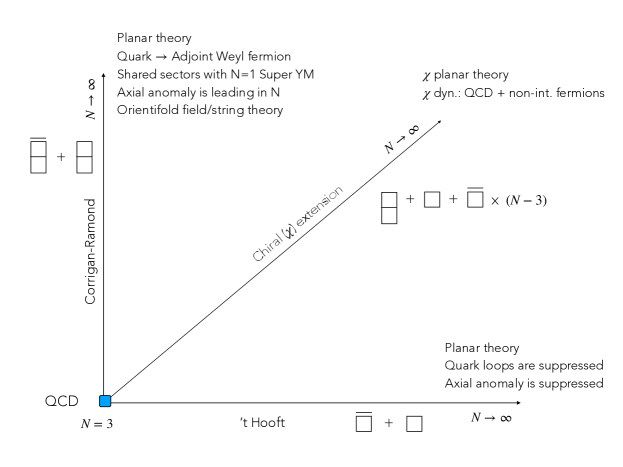
Figure 1: Diagram summarizing the three large $\displaystyle N$ QCD extensions, their matter contents and salient large $\displaystyle N$ properties. This is the improved version of the similar figure first appeared in our earlier work Ryttov:2005na .

Focusing on the CR limit, but simultaneously considering also two-index symmetric theories it was later shown by Armoni, Shifman and Veneziano Refs. Armoni:2003gp ; Armoni:2003fb that there is a planar connection among the mesonic sectors of these theories and $\displaystyle\mathcal{N}=1$ super Yang-Mills theory. The two-index theories are also known in string-theory as orientifold theories since they were shown to live on a brane configuration of type 0A string theory Armoni:1999gc ; Angelantonj:1999qg consisting of NS5 branes, D4 branes and an orientifold plane. It is useful to summarize the perturbative spectrum of the two-orientifold theories in the table 1.

	$\displaystyle SU(N)$	$\displaystyle U_{V}(1)$	$\displaystyle U_{A}(1)$
$\displaystyle{\psi_{\{ij\}}}$		$\displaystyle 1$	$\displaystyle 1$
$\displaystyle\widetilde{\psi}^{\{ij\}}$	$\displaystyle\overline{\raisebox{-0.5pt}{\hbox{\rule{0.4pt}{6.5pt}\hskip-0.4pt\rule{6.5pt}{0.4pt}\hskip-6.5pt\rule[6.5pt]{6.5pt}{0.4pt}}\rule[6.5pt]{0.4pt}{0.4pt}\hskip-0.4pt\rule{0.4pt}{6.5pt}}\hskip-0.4pt\raisebox{-0.5pt}{\hbox{\rule{0.4pt}{6.5pt}\hskip-0.4pt\rule{6.5pt}{0.4pt}\hskip-6.5pt\rule[6.5pt]{6.5pt}{0.4pt}}\rule[6.5pt]{0.4pt}{0.4pt}\hskip-0.4pt\rule{0.4pt}{6.5pt}}}$	$\displaystyle-1$	$\displaystyle 1$
$\displaystyle G_{\mu}$	Adj	$\displaystyle 0$	$\displaystyle 0$

	$\displaystyle SU(N)$	$\displaystyle U_{V}(1)$	$\displaystyle U_{A}(1)$
$\displaystyle\psi_{[ij]}$		$\displaystyle 1$	$\displaystyle 1$
$\displaystyle\widetilde{\psi}^{[ij]}$	$\displaystyle\overline{\vbox{\vbox{\hrule height=0.3pt\hbox{\vrule width=0.3pt,height=6.4pt\kern 6.4pt\vrule width=0.3pt} \hrule height=0.3pt\kern-0.3pt\hrule height=0.3pt\hbox{\vrule width=0.3pt,height=6.4pt\kern 6.4pt\vrule width=0.3pt} \hrule height=0.3pt}}}$	$\displaystyle-1$	$\displaystyle 1$
$\displaystyle G_{\mu}$	Adj	$\displaystyle 0$	$\displaystyle 0$

Table 1: The table summarizes the perturbative spectrum of the (anti) symmetric orientifold theories in the (right) left part of the table. $\displaystyle\psi$ and $\displaystyle\widetilde{\psi}$ are two Weyl fermions, while $\displaystyle G_{\mu}$ indicates the gauge bosons. $\displaystyle U_{V}(1)$ is the conserved vector global symmetry while the $\displaystyle U_{A}(1)$ symmetry is broken by the chiral quantum anomaly.

The subtle issues of the confinement properties stemming from the centre group symmetries and (in)equivalences at finite and large $\displaystyle N$ were discussed first in Ref. Sannino:2005sk . The large $\displaystyle N$ planar equivalence means that some of the super Yang-Mills exact results, such as the ones found in Shifman:1999mv ; Shifman:1987ia can be exported to the infinite $\displaystyle N$ limit of the orientifold theories. For example, the orientifold theories, at large $\displaystyle N$, have an exactly calculable bifermion condensate and an infinite number of degeneracies in the spectrum of color-singlet hadrons. Some of the finite $\displaystyle N$ implications of the correspondence were developed in Sannino:2003xe . The corrections were deduced by matching the infinite $\displaystyle N$ effective theory describing the lowest lying composite states associated to the fluctuations of the fermion condensate with the bosonic sector of the Veneziano and Yankielowicz (VY) Veneziano:1982ah effective theory for super Yang-Mills. By considering $\displaystyle 1/N$ supersymmetry breaking effects, as well as the explicit ones due to the introduction of a finite quark mass, several predictions were made in Sannino:2003xe concerning the spectrum of the low-lying mesonic states, the gluon condensate, the $\displaystyle\theta$-angle physics as well as the vacuum energy. In particular we computed the pseudo-scalar to scalar mass ratio at finite number of colors and at finite quark mass for the orientifold field theories.

Capitalizing on the work on orientifold field theories via their description in terms of $\displaystyle O^{\prime}$ string theory of DiVecchia:2004hvn ; DiVecchia:2005vm the same pseudo-scalar to scalar mass ratio was discussed in Armoni:2005qr for the fermion massless limit. I will comment later about the different approximations that went in this analysis including the caveat on how to interpret the computations in the closed string sector DiVecchia:2004hvn ; DiVecchia:2005vm .

Intriguingly, as suggested in Sannino:2005sk ; Feo:2004mr , one can flip the point of view and use QCD or $\displaystyle SU(N)$ with higher values of $\displaystyle N$ for the two-index symmetric theories to acquire information about super Yang-Mills. Here I have in mind not only the (pseudo) scalar spectrum of the theory but also higher spin and excited states Ziegler:2021nbl ; DellaMorte:2023ylq . In fact, these sectors have eluded the power of supersymmetry and are relevant for model building. Additionally, assuming that our suggestion, i.e. the non-perturbative dynamics of chiral gauge theories reduces in the infrared to the one of a strongly coupled vector core augmented by a non-interacting chiral one, holds true one can also determine the non-perturbative spectrum of chiral gauge theories.

Recent lattice simulations for ordinary one flavour QCD Ziegler:2021nbl ; Jaeger:2022ypq ; DellaMorte:2023ylq ; DellaMorte:2023sdz provide results that can be directly compared with the original predictions Sannino:2003xe . Of course, this is not the first time that one flavor QCD has been studied numerically. In fact, general features of the theory were discussed in Creutz:2006ts . The quark condensate was computed in DeGrand:2006uy by comparing the density of low-lying eigenvalues of the overlap Dirac operator to predictions from Random Matrix Theory Leutwyler:1992yt ; Shuryak:1992pi . The results are in agreement with the predictions for the gluino condensate obtained in Armoni:2003yv although sizable $\displaystyle 1/N$ corrections are expected Sannino:2003xe . Using Wilson fermions the authors of reference Farchioni:2007dw had provided a preliminary investigation of the low-lying mesonic spectrum of one-flavor QCD. The latter was improved in in Ziegler:2021nbl ; Jaeger:2022ypq ; DellaMorte:2023ylq ; DellaMorte:2023sdz via finer lattice spacing, larger volumes and a tree-level improved fermionic action. Recently the glueball spectrum has been discussed in Athenodorou:2023xdi . Reducing the numbers of colors to two colors the one flavor case was investigated in Francis:2018xjd . This theory is phenomenologically interesting as composite Dark Matter model. Due to the fact that the fundamental representation of $\displaystyle SU(2)$ is pseudo-real the global $\displaystyle U(1)$ vector symmetry is enhanced to $\displaystyle SU(2)$. Interestingly, the dark matter model envisioned in Francis:2018xjd features a mass-gap with vector mesons being the lightest triplet of the enhanced $\displaystyle SU(2)$ global symmetry. The latter is a spectral feature shared with the dark matter model based also on an $\displaystyle SU(2)$ gauge theory but featuring scalar quarks Hambye:2009fg . The $\displaystyle SU(2)$ theory with one Dirac adjoint fermion was investigated, adopting the Wilson Dirac operator, in  Athenodorou:2021wom to elucidate the onset of the conformal window for higher dimensional representations Sannino:2004qp ; Dietrich:2006cm . The first study of composite dark matter via lattice study appeared in Lewis:2011zb for $\displaystyle SU(2)$ with two Dirac fermions. In fact, this theory is one of the most revealing and central a minimal template for composite dynamics for beyond standard model physics as summarized in Cacciapaglia:2020kgq . For a detailed discussion about the methodologies used on the lattice and their limits the reader will find a detailed account in Ziegler:2021nbl ; Jaeger:2022ypq ; DellaMorte:2023ylq ; DellaMorte:2023sdz . The issues related to the use of Wilson fermions are further discussed in  Edwards:1997sp ; Edwards:1998sh ; Akemann:2010em ; Mohler:2020txx ; Bergner:2011zp . I further recall that earlier investigations of orientifold theories Lucini:2010kj ; Armoni:2008nq were performed via quenched approximations avoiding the sign problem but also naturally suppressing fermion loops which is more in line with the ’t Hooft large $\displaystyle N$ limit. We complete our excursion in lattice land by recalling that numerical simulations of supersymmetric gauge theories have a long history Catterall:2009it with a recent review Schaich:2022xgy discussing the status and open challenges.

The remainder is organized as follows. In Section 2 I review the effective orientifold lagrangian of Sannino:2003xe and briefly summarize the rationale behind its construction. I then report the $\displaystyle 1/N$ predictions of the vacuum and spectral properties of the orientifold field theories. Retracing the steps of Sannino:2003xe , I write the physical quantities directly in terms of the trace and axial anomalies in units of the super Yang-Mills ones. The rewriting not only allows to better visualize the origin of the finite $\displaystyle N$ deformations from super Yang-Mills but also to arrive at an improved version of the pseudo-scalar to scalar mass ratio which, of course, returns the original result Sannino:2003xe when restricting it to the $\displaystyle 1/N$ corrections. The leading $\displaystyle 1/N$ and improved predictions are then confronted with the lattice results of DellaMorte:2023ylq showing the remarkable fact that the improved results are about one standard deviation away from the lattice central result. By comparing with the leading $\displaystyle 1/N$ result I estimate the size of the $\displaystyle 1/N^{2}$ corrections. Section 4 reviews the impact of a small fermion mass operator on the spectrum. We argue that by testing the mass dependence of the pseudoscalar to scalar ratio constitutes an independent direct test of the infinite $\displaystyle N$ supersymmetric connection. This is so since, at leading order in the fermion mass, the corrections are protected by supersymmetry because the mass operator is a soft susy breaking one Masiero:1984ss . In section 5 we comment on the string theory inspired computation of the pseudoscalar to scalar mass ratio at zero fermion mass. We then move up in the number of flavors and step away from super Yang Mills. Having learnt already so much about the alternative large $\displaystyle N$ limit we are ready to review its impact on non-perturbative scattering dynamics of two-index symmetric representations with more than one Dirac flavor Kiritsis:1989ge ; Sannino:2007yp . Here we finally address Weinberg’s point by showing that the CR extrapolation more effectively unitarize $\displaystyle\pi\pi$ scattering than the ’t Hooft limit. Additionally, we will see that tetraquark mesonic states appear already at leading order in $\displaystyle N$ in the CR limit. We offer our conclusions in section 7.

2 Spectrum and vacuum properties via the Effective Orientifold Theory

Effective Lagrangians describing the vacuum properties of strongly coupled gauge theories respective the underlying trace and axial variations have a long history Schechter:1980ak ; Rosenzweig:1979ay ; DiVecchia:1980yfw ; Kawarabayashi:1980dp ; Migdal:1982jp ; Cornwall:1983zb . Here we will consider the effective Lagrangian for the finite $\displaystyle N$ orientifold field theory constructed in Sannino:2003xe which reads:

$${\cal L}_{\rm eff}=f(N)\left\{\frac{1}{\alpha}\left(\varphi\,\bar{\varphi}\right)^{-2/3}\,\partial_{\mu}\bar{\varphi}\,\partial^{\mu}\varphi-\frac{4\alpha}{9}\,\left(\varphi\,\bar{\varphi}\right)^{2/3}\,\left(\ln\bar{\Phi}\,\ln\Phi-b\right)\right\}\,.$$ (1)

The field $\displaystyle\varphi$ encodes information about the fermion bilinear

$$\displaystyle\varphi=-\frac{3}{32\pi^{2}\,N}\,\widetilde{\psi}^{\alpha,[i,j]}\psi_{\alpha,[i,j]}\ .$$ (2)

We have set the infinite $\displaystyle N$ gluino condensate scale $\displaystyle\Lambda=1$ to keep the notation light but it will re-inserted later when discussing the physical spectrum. $\displaystyle b\sim{\cal O}(1/N)$ is a numerical (real) positive parameter as argued in Sannino:2003xe by comparing to the QCD gluon condensate and vacuum energy, $\displaystyle f(N)\rightarrow N^{2}$ at $\displaystyle N\rightarrow\infty$ and

$$\Phi=\varphi^{1+\epsilon_{1}}\,\bar{\varphi}^{-\epsilon_{2}}\,,\qquad\bar{\Phi}=\bar{\varphi}^{1+\epsilon_{1}}\,\varphi^{-\epsilon_{2}}\,,$$ (3)

where $\displaystyle\epsilon_{1,2}$ are subleading in $\displaystyle 1/N$ parameters allowing for distinct finite $\displaystyle N$ corrections stemming from the scale and chiral anomalies. In fact, varying the effective oreintifold actions under scale $\displaystyle\varphi\to(1+3\gamma)\varphi$ and chiral $\displaystyle\varphi\to(1+2i\gamma)\varphi$ transformations with respect to the real parameter $\displaystyle\gamma$ one obtains the following scale and chiral transformation at the effective action level:

$$\displaystyle\delta{\cal S}_{\rm eff}^{\rm scale} \displaystyle= \displaystyle\int d^{4}x\left\{-4\,\frac{\alpha\,f}{3}\left(\varphi\,\bar{\varphi}\right)^{2/3}\left(1+\epsilon_{1}-\epsilon_{2}\right)\left(\ln\bar{\Phi}+\ln\Phi\right)\right\}\,,$$ (4)

$$\displaystyle\delta{\cal S}_{\rm eff}^{\rm chiral} \displaystyle= \displaystyle\int d^{4}x\left\{-8i\,\,\frac{\alpha\,f}{9}\left(\varphi\,\bar{\varphi}\right)^{2/3}\left(1+\epsilon_{1}+\epsilon_{2}\right)\left(\ln\bar{\Phi}-\ln\Phi\right)\right\}\,.$$ (5)

To deduce the epsilon parameters we need to compare them to the trace and axial anomalies at the fundamental lagrangian level:

$$\displaystyle\vartheta^{\mu}_{\mu} \displaystyle= \displaystyle\frac{\beta_{O\pm}(a)}{a^{2}}\frac{1}{32\pi^{2}}\,G_{\mu\nu}^{a}{G}^{a,\,\mu\nu}$$ (6)

$$\displaystyle\partial^{\mu}J_{\mu} \displaystyle= \displaystyle\left[N\pm 2\right]\frac{1}{16\pi^{2}}\,G_{\mu\nu}^{a}{\tilde{G}}^{a,\,\mu\nu}\ .$$ (7)

Here $\displaystyle\beta_{O\pm}$ are the beta functions for the orientifold field theories with the generic beta function defined, in perturbation theory, as:

$$\frac{d\,a}{d\ln\mu^{2}}\equiv\beta_{O\pm}(a)=-\beta_{0}a^{2}-\beta_{1}a^{3}-\beta_{2}a^{4}\cdots\ ,\quad{\rm with}\quad a=g^{2}/(4\pi)^{2}\ .$$ (8)

Additionally by comparison between the underlying and effective anomaly variations we have Sannino:2003xe :

$$\displaystyle G_{\mu\nu}^{a}{G}^{a,\,\mu\nu} \displaystyle\propto \displaystyle-N\left(\varphi\,\bar{\varphi}\right)^{2/3}\left(\ln\bar{\Phi}+\ln\Phi\right)\,,$$

$$\displaystyle G_{\mu\nu}^{a}\tilde{G}^{a,\,\mu\nu} \displaystyle\propto \displaystyle-N\,i\,\left(\varphi\,\bar{\varphi}\right)^{2/3}\left(\ln\bar{\Phi}-\ln\Phi\right)\,.$$ (9)

Once properly normalized to the super Yang-Mills limit we have:

$$1+\epsilon_{1}+\epsilon_{2}\equiv{\chi}=\frac{N\pm 2}{N}\ ,\qquad 1+\epsilon_{1}-\epsilon_{2}\equiv{\cal T}=\frac{\beta_{O\pm}(a)}{\beta_{SYM}(a)}=-\frac{1}{3N}\frac{\beta_{O\pm}(a)}{a^{2}}\ ,$$ (10)

yielding:

$$2\epsilon_{2}=\chi-{\cal T}\ ,\qquad\epsilon_{1}=1-\frac{\chi+{\cal T}}{2}\ .$$ (11)

By construction both epsilons start at the order $\displaystyle 1/N$ when moving away from super Yang-Mills. Once minimized the effective orientifold action returns the following vacuum energy density:

$$V_{\rm min}={\cal E}_{\rm vac}=-\frac{4\alpha\,f}{9}\,b+O(N^{0})\,.$$ (12)

As we mentioned earlier the sign of $\displaystyle b$ is consistent, for the two-index antisymmetric orientifold theory, with the fact that for QCD with three light flavors the gluon condensate is positive and the vacuum energy density is negative Shifman:1978bx . One flavor QCD is obtained by decoupling two light quarks affecting the absolute value of the gluon condensate but not its sign Novikov:1981xi . For further arguments related to the sign of $\displaystyle b$ associated, for example, to pure gluon-dynamics we refer to Sannino:2003xe .

Approaching super Yang-Mills when increasing the number of colors leads to spectral degenaracies for the orientifold theories dictated by super symmetry and reflected in the effective orientifold Lagrangian by the degeneracy between the scalar $\displaystyle\sigma$ and the pseudoscalar $\displaystyle\eta^{\prime}$ mesons. Studying the spectrum of fluctuations related to $\displaystyle\varphi$ as $\displaystyle\displaystyle{\varphi=\langle\varphi\rangle\left(1+c\,h\right)}$ with $\displaystyle\displaystyle{h=\frac{1}{\sqrt{2}}\left(\sigma+i\,\eta^{\prime}\right)}$ and $\displaystyle\displaystyle{c^{2}=\frac{\alpha}{f}\,|\langle\varphi\rangle|^{-\frac{2}{3}}}$ we obtained in Sannino:2003xe :

$$\displaystyle M_{\sigma} \displaystyle= \displaystyle\frac{2\alpha}{3}\,{\Lambda}\,(1+\frac{2}{9}b)\,\left[1+\epsilon_{1}-\epsilon_{2}+\frac{4}{9}b\right]=\frac{2\alpha}{3}\,{\Lambda}\,(1+\frac{2}{9}b)\,\left[{\cal T}+\frac{4}{9}b\right],$$

$$\displaystyle M_{\eta^{\prime}} \displaystyle= \displaystyle\frac{2\alpha}{3}\,{\Lambda}\,(1+\frac{2}{9}b)\,\left[1+\epsilon_{1}+\epsilon_{2}\right]=\frac{2\alpha}{3}\,{\Lambda}\,\,(1+\frac{2}{9}b)\,\chi\ ,$$ (13)

where in the last equality we expanded at leading order in $\displaystyle 1/N$. In fact it is not necessary to make this expansion when considering the ratio of the masses. At infinite number of colors the $\displaystyle b$ coefficient vanishes and $\displaystyle{\cal T}=\chi=1$ and we recover the supersymmetric limit $\displaystyle\displaystyle{M_{\sigma}=M_{\eta}^{\prime}=\frac{2\alpha}{3}\Lambda}$. The vacuum parameter $\displaystyle b$ beyond the overall redefinition of $\displaystyle\Lambda$ for both physical states it further affects directly the mass of the scalar state since the latter has the same quantum numbers of the vacuum, however it does not contribute to the pseudo-scalar state because the orientifold theory is parity invariant.

The finite $\displaystyle N$ ratio of the pseudoscalar to scalar mass is

$$\displaystyle\frac{M_{\eta^{\prime}}}{M_{\sigma}}=\frac{\chi}{{\cal T}+\frac{4}{9}b}=\frac{1\pm{2}/{N}}{{\beta_{O\pm}}/{\beta_{SYM}}+\frac{4}{9}b}\leq\frac{1\pm{2}/{N}}{{\beta_{O\pm}}/{\beta_{SYM}}}\ .$$ (14)

Considering only the leading $\displaystyle 1/N$ corrections we recover the result of Sannino:2003xe

$$\displaystyle\frac{M_{\eta^{\prime}}}{M_{\sigma}}={1+2\epsilon_{2}-\frac{4}{9}b}+{\cal O}(1/N^{-2})=1+\chi-{\cal T}-\frac{4}{9}b+{\cal O}(1/N^{-2})\ ,$$ (15)

where in the last equality we keep only the leading $\displaystyle 1/N$ corrections in the $\displaystyle\chi-{\cal T}$ term. Clearly equation (15) holds in the vicinity of $\displaystyle N\rightarrow\infty$ while we expect equation (14) to better capture the general features of this ratio for smaller values of $\displaystyle N$.

To be predictive one can now estimate the ratio $\displaystyle\beta_{O\pm}/\beta_{SYM}$. In Sannino:2003xe we employed the one loop beta function coefficients. The rationale for this choice is that, in the Wilsonian regularization scheme used to write the VY effective action for super Yang-Mills the beta function is one loop exact. In turns, this ensures that the effective potential of the effective supersymmetric action is holomorhpic. Therefore, when going away from the supersymmetric limit it is natural to start with the one loop coefficient of the orientifold beta functions that captures in a simple manner deviations from holomorphicity yielding

$${\cal T}=\frac{\beta_{O\pm}}{\beta_{SYM}}=1\mp\frac{4}{9N}\qquad{\rm one\leavevmode\nobreak\ loop}\ .$$ (16)

Expanding around the infinite $\displaystyle N$ result and retaining only the $\displaystyle 1/N$ corrections one recovers the result of Sannino:2003xe which is:

$$\displaystyle\frac{M_{\eta^{\prime}}}{M_{\sigma}}\Big{|}_{O\pm}=1+\chi-{\cal T}-\frac{4}{9}b+{\cal O}(1/N^{-2})=1\pm\frac{22}{9N}-\frac{4}{9}b+{\cal O}(1/N^{-2})\ .$$ (17)

Needless to say, this result is valid only in the asymptotically large number of colors and direct comparison for small $\displaystyle N$ are subject to large corrections. If one insists in trying to access smaller values of $\displaystyle N$ it should be better to compare to (14):

$$\displaystyle\frac{M_{\eta^{\prime}}}{M_{\sigma}}\Big{|}_{O\pm}=\frac{\chi}{{\cal T}+\frac{4}{9}b}\,\leq\frac{1\pm{2}/{N}}{1\mp\frac{4}{9N}}\ ,$$ (18)

which, of course, recovers the expected large $\displaystyle N$ subleading terms of Sannino:2003xe and better captures finite $\displaystyle N$ corrections, as we shall momentarily see, when comparing the prediction to lattice data Ziegler:2021nbl ; Jaeger:2022ypq ; DellaMorte:2023ylq ; DellaMorte:2023sdz . I term the ratio in (18) the finite $\displaystyle N$ improved result.

3 Comparing to lattice results and the size of the $\displaystyle 1/N^{2}$ corrections

For three colors the two-index antisymmetric theory is one flavor QCD for which the $\displaystyle 1/N$ and the improved results give respectively

$$\frac{M_{\eta^{\prime}}}{M_{\sigma}}\Big{|}_{\rm QCD-leading}\leq 0.185\leavevmode\nobreak\ {\rm up\leavevmode\nobreak\ to\leavevmode\nobreak\ }{\cal O}(N^{-2})\quad{\rm and}\quad\frac{M_{\eta^{\prime}}}{M_{\sigma}}\Big{|}_{\rm QCD-improved}\leq 0.290\ .$$ (19)

The predictions should be compared to the lattice value $\displaystyle 0.356(54)$ computed in DellaMorte:2023ylq ; DellaMorte:2023sdz . The latter is compatible with the improved result within two sigma confidence level. In figure 2 I plot our predictions for the pseudoscalar to scalar mass ratio as function of the number of colors for both, the two-index symmetric (blue curves) and antisymmetric case (red curves). The dashed curves correspond to the leading $\displaystyle 1/N$ corrections while the solid ones are for the improved version. The lattice result for one-flavor QCD is shown in the plot for $\displaystyle N=3$ at the two sigma confidence level.

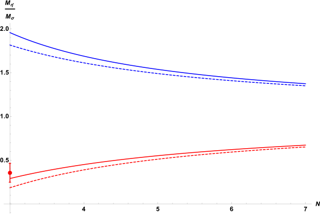
Figure 2: Predictions for the pseudoscalar to scalar mass ratio as function of the number of colors $\displaystyle N$ for the two-index symmetric, upper blue solid and dashed curves, and two-index antisymmetric as lower red solid and dashed curves. The solid lines are due to (18) while the dashed lines come from (14). The lattice result, for one-flavor QCD, is shown at two sigma confidence level.

Given the remarkable success it is tempting to assume the improved expression

$$\displaystyle\frac{M_{\eta^{\prime}}}{M_{\sigma}}=\frac{\chi}{{\cal T}+\frac{4}{9}b}=\frac{1\pm{2}/{N}}{{\beta_{O\pm}}/{\beta_{SYM}}+\frac{4}{9}b}\ ,$$ (20)

to be valid for any $\displaystyle N$. After all, the numerator coefficient, that stems from the axial anomaly, is all-order exact and we have seen that mild assumptions on the ratio of beta functions leads to surprisingly consistent results with first principle lattice simulations even for small number of colors while naturally interpolating with the leading $\displaystyle 1/N$ corrections.

It is natural to ask what happens if one were to depart from the Wilsonian scheme for the beta functions. One way to illustrate this is to consider the universal two-loop beta ratio expanded in $\displaystyle 1/N$ which yields:

$${\cal T}=\frac{\beta_{O\pm}}{\beta_{SYM}}=1\mp\frac{4}{9N}\frac{1+\frac{19}{4}\lambda}{1+\lambda}\quad{\rm with}\quad\lambda=\frac{Ng^{2}}{8\pi^{2}}\ .$$ (21)

Here $\displaystyle\lambda$ is the ’t Hooft coupling and one can easily check that the result is consistent with the all-order NVSZ super Yang-Mills beta function Novikov:1983uc ; Shifman:1986zi . One can always find a scheme were the two-loop is all there is. In this case the largest modification occurs for the largest value of $\displaystyle\lambda$ giving $\displaystyle{\cal T}=1\mp 19/(9N)$ and an upper limit for the QCD ration of 0.196 which is slightly higher than the leading $\displaystyle N$ one, again speaking in favour of the robustness of the results.

We now use the lattice results to estimate the size of the $\displaystyle 1/N^{2}$ by extending (22) to

$$\displaystyle\frac{M_{\eta^{\prime}}}{M_{\sigma}}\Big{|}_{O\pm}=1+\chi-{\cal T}-\frac{4}{9}b+{\cal O}(1/N^{-2})=1\pm\frac{22}{9N}-\frac{4}{9}b+\frac{\kappa}{N^{2}}+{\cal O}(1/N^{-3})\ ,$$ (22)

and obtain $\displaystyle\kappa\geq 1.54$ with the equality holding for $\displaystyle b=0$. For a reasonable positive non vanishing value of $\displaystyle b\approx 1/N$ we find $\displaystyle\kappa\approx 2.87$.

4 The quark mass weighs in

In Sannino:2003xe we followed Masiero and Veneziano Masiero:1984ss in adding a supersymmetry breaking term stemming from the gluino mass $\displaystyle m$ translating into adding in the initial the Lagrangian the last operator below:

$$f(N)\left\{\frac{1}{\alpha}\left(\varphi\,\bar{\varphi}\right)^{-2/3}\,\partial_{\mu}\bar{\varphi}\,\partial^{\mu}\varphi-\frac{4\alpha}{9}\,\left(\varphi\,\bar{\varphi}\right)^{2/3}\,\left(\ln\bar{\Phi}\,\ln\Phi-\beta\right)\right\}+\frac{4\,m}{3\lambda}\,N^{2}\left(\varphi+\bar{\varphi}\right)\ .$$ (23)

This yields the following vacuum energy:

$$\displaystyle{\cal E}_{\rm vac}=V_{\rm min}=-\frac{4\alpha f}{9}\beta\Lambda^{4}-\frac{8N^{2}}{3\lambda}m\Lambda^{3}+{O}\left(m^{2},N^{0},mN\right)\ .$$ (24)

and the leading $\displaystyle 1/N$ and $\displaystyle m$ spectrum for the ratio of the pseudoscalar to scalar mass one has:

$$\displaystyle\frac{M_{\eta^{\prime}}}{M_{\sigma}}=1-\frac{22}{9N}-\frac{4}{9}\beta-\frac{m}{\alpha\lambda\Lambda}+{O}(m^{2},N^{-2},mN^{-1})\ .$$ (25)

The improved finite $\displaystyle N$ but small fermion mass version is

$$\displaystyle\frac{M_{\eta^{\prime}}}{M_{\sigma}}\Big{|}_{\rm improved}=\frac{1\pm{2}/{N}}{{\beta_{O\pm}}/{\beta_{SYM}}+\frac{4}{9}b}-\frac{m}{\alpha\lambda\Lambda}+{O}(m^{2})\ .$$ (26)

The gluon condensate becomes:

$$\displaystyle\frac{\langle G^{a}_{\mu\nu}G^{a,\mu\nu}\rangle}{64\pi^{2}}=\frac{4\,N\,m}{3\lambda}\,\Lambda^{3}+\frac{8}{27}\alpha\,N\beta\Lambda^{4}+{O}\left(m^{2},N^{-1},mN^{0}\right)\ .$$ (27)

These results show that the contribution of the fermion mass reinforces the effect of the finite $\displaystyle N$ contribution in decreasing the ratio of the pseudo-scalar to scalar masses.

The $\displaystyle\theta$-angle dependence of the vacuum energy for the fermions in the two-index antisymmetric representation of the gauge group is

$$\displaystyle{\cal E}_{\rm vac}=\frac{8N^{2}}{3\,\lambda}\,m\Lambda^{3}\,{\rm min}_{k}\left\{-\cos\left[\frac{\theta+2\pi\,k}{N-2}\right]\right\}-\frac{4\alpha f}{9}\beta\Lambda^{4}\ .$$ (28)

The $\displaystyle N-2$-fold vacuum degeneracy is lifted due to the presence of a mass term in the theory, yielding a unique vacuum.

5 Comments on a string theory inspired perspective

Using a string inspired approach the authors of reference Armoni:2005qr provided an alternative estimate for the pseudo-scalar to scalar mass ratio above by arguing in favour of setting $\displaystyle{\cal T}+\frac{4}{9}b\approx 1$ while keeping $\displaystyle\chi=1\pm 2/N$. This choice corresponds, in the effective Lagrangian approach, to have the scalar mass fixed at the SUSY value and therefore only the axial anomaly is responsible for the finite $\displaystyle N$ corrections, arriving at

$$\frac{M_{\eta^{\prime}}}{M_{\sigma}}\Big{|}_{\rm String}\approx\chi=1\pm\frac{2}{N}\ .$$ (29)

I will now briefly review the assumptions made in Armoni:2005qr and highlight the various caveats. The first intuition is that one can extract information about orientifold field theories via their description in terms of $\displaystyle O^{\prime}$ string theory of DiVecchia:2004hvn ; DiVecchia:2005vm . By determining the string annulus partition function in presence of external gauge fields for the open and close string sectors in DiVecchia:2004hvn ; DiVecchia:2005vm the coefficients for the axial and trace anomalies were determined. The axial coefficients were computed to be identical for both the closed and opened string sectors naturally matching the exact field theoretical result while the trace anomaly coefficients differ, with the open strings yielding the one-loop result for orientifold field theories and the closed sector giving the supersymmetric result. Naturally, the authors of DiVecchia:2004hvn ; DiVecchia:2005vm attributed the discrepancy, in computing the coefficient of the trace anomaly, in the open and closed string sectors to the missing of threshold corrections in the closed sector. In fact, both sectors should return the perturbative field theoretical result. Despite this warning, the authors in Armoni:2005qr elevated the incomplete closed string result to a genuine non-perturbative prediction of trace anomaly for the orientifold field theory. A second assumption is that the pure (pseudo) glueball point function is saturated by the (pseudo) scalar state assuming that these are the lightest states. This assumption is partially justified by the studies in Merlatti:2004df ; Feo:2004mr . In these papers the effective Lagrangians included besides the (pseudo) scalar states made by fermions also the (pseudo) glueball states and computed their mixing. The last assumption Armoni:2005qr is to neglect extra $\displaystyle{\cal O}(1/N)$ corrections in any other existing parameter entering the ratio of the two-point functions except for the coefficient of the axial anomaly. Overall, seen from the effective orientifold theory computation, the approximations above amount at considering only the corrections for the pseudoscalar state (stemming from axial anomaly) while the scalar state remains unperturbed from the super Yang-Mills limit which would be surprising. Nevertheless, given that one of the strongest assumptions is associated to the string theory description, it would be interesting to have a complete computation for the closed sector of $\displaystyle O^{\prime}$ string theory. Of course, a direct comparison with the lattice data, even if they superficially seem to be a better fit still begs the question of why the $\displaystyle 1/N^{2}$ corrections should be so much suppressed.

6 Tetraquark mesons and $\displaystyle\pi\pi$ scattering at large $\displaystyle N$, explained

I can now comment on Weinberg’s work Weinberg:2013cfa about large $\displaystyle N$ meson-meson scattering and tetraquarks. These two quantities are naturally related since tetraquarks can appear as intermediate states in the $\displaystyle\pi\pi$ scattering amplitude. Upon analyzing the tetraquark contribution to meson-meson scattering and their propagators, Coleman Coleman_1985 correctly argues that, in the leading $\displaystyle N$ ’t Hooft limit, these states do not appear in meson-meson scattering and furthermore the connected component of their propagator is also suppressed. In Coleman’s own words: In the large $\displaystyle N$ limit, quadrilinear make meson pairs and nothing else. Weinberg challenges this statement and writes: But is this justified?. Rather than answering the question at the scattering amplitude level he considers the decay width instead. Weinberg furthermore argues that Coleman’s conclusion could be reasonable if the decay width into ordinary mesons grows with $\displaystyle N$, justifying why a tetraquark may not be observable as a distinct particle. He then argues that the width decreases with $\displaystyle N$ instead. Weinberg interprets his result as a way to justify the presence of tetraquarks even in the ’t Hooft limit. However, this is not entirely correct, since the mass of the tetrquarks could be not leading in $\displaystyle N$ and some tetraquarks can still remain broad, like the $\displaystyle f_{0}(500)$.

In the following I will show, at the meson-meson scattering amplitude level, that the alternative large $\displaystyle N$ limit is better suited than the ’t Hooft extrapolation to address the issues above. Because I wish to discuss phenomenologically relevant scattering amplitudes I add light flavors. Although, in this case, the large $\displaystyle N$ theories depart from the supersymmetric Yang-Mills limit, one can still employ the CR large $\displaystyle N$ to access information complementary to the ’t Hooft limit Kiritsis:1989ge ; Sannino:2007yp . A noteworthy example is the celebrated $\displaystyle\pi\pi$ scattering amplitude Sannino:2007yp . To this end I recall that for quarks in the two-index representation the large $\displaystyle N$ diagram for the quark-quark gluon interaction is the one in Fig. 3.

every picture/.style=line width=0.7pt

[x=0.75pt,y=0.75pt,yscale=-1,xscale=1]

[fill=rgb, 255:red, 0; green, 0; blue, 0 ,fill opacity=1 ] (186.63,194.32) – (170.19,200.17) – (169.51,190.94) – cycle ; [fill=rgb, 255:red, 0; green, 0; blue, 0 ,fill opacity=1 ] (265.61,193.38) – (249.12,199.12) – (248.5,189.88) – cycle ; (145,195.35) – (288,193.65) ; (216.01,194.12) .. controls (214.04,195.15) and (212.17,196.14) .. (212.17,197.27) .. controls (212.18,198.41) and (214.06,199.38) .. (216.04,200.4) .. controls (218.01,201.41) and (219.89,202.39) .. (219.9,203.52) .. controls (219.9,204.66) and (218.03,205.65) .. (216.06,206.68) .. controls (214.1,207.71) and (212.22,208.7) .. (212.23,209.83) .. controls (212.23,210.97) and (214.11,211.94) .. (216.09,212.96) .. controls (218.07,213.97) and (219.95,214.95) .. (219.95,216.08) .. controls (219.96,217.22) and (218.09,218.21) .. (216.12,219.24) .. controls (214.15,220.27) and (212.28,221.26) .. (212.28,222.39) .. controls (212.29,223.53) and (214.17,224.5) .. (216.15,225.52) .. controls (218.12,226.53) and (220,227.51) .. (220.01,228.64) .. controls (220.01,229.78) and (218.14,230.77) .. (216.17,231.8) .. controls (214.21,232.83) and (212.33,233.82) .. (212.34,234.95) .. controls (212.34,236.09) and (214.22,237.06) .. (216.2,238.08) .. controls (218.18,239.09) and (220.06,240.07) .. (220.06,241.2) .. controls (220.07,242.34) and (218.2,243.33) .. (216.23,244.36) .. controls (214.26,245.39) and (212.39,246.38) .. (212.39,247.51) .. controls (212.4,248.65) and (214.28,249.62) .. (216.26,250.64) .. controls (218.23,251.66) and (220.11,252.63) .. (220.12,253.76) .. controls (220.12,254.9) and (218.25,255.89) .. (216.28,256.92) .. controls (214.32,257.95) and (212.44,258.94) .. (212.45,260.07) .. controls (212.45,261.21) and (214.33,262.18) .. (216.31,263.2) .. controls (217.14,263.63) and (217.96,264.05) .. (218.62,264.48) ;

(300,223) – (312.5,215) – (312.5,219) – (337.5,219) – (337.5,215) – (350,223) – (337.5,231) – (337.5,227) – (312.5,227) – (312.5,231) – cycle ; [fill=rgb, 255:red, 0; green, 0; blue, 0 ,fill opacity=1 ] (410.22,190.47) – (395.29,194.57) – (395.14,186.87) – cycle ; [fill=rgb, 255:red, 0; green, 0; blue, 0 ,fill opacity=1 ] (470.37,189.67) – (455.42,193.71) – (455.31,186) – cycle ; (365.5,191.1) – (493,189.53) ; (368.17,203.85) – (426.13,204.59) ; (426.79,256.17) – (425.82,204.12) ; (440.08,255.42) – (439.19,205.37) ; (439.02,204.35) – (492.53,203.09) ; [fill=rgb, 255:red, 0; green, 0; blue, 0 ,fill opacity=1 ] (410.22,204.21) – (395.29,208.32) – (395.14,200.61) – cycle ; [fill=rgb, 255:red, 0; green, 0; blue, 0 ,fill opacity=1 ] (471.26,203.83) – (456.32,207.87) – (456.2,200.16) – cycle ; [fill=rgb, 255:red, 0; green, 0; blue, 0 ,fill opacity=1 ] (426.28,243.81) – (421.39,230.02) – (429.63,229.62) – cycle ; [fill=rgb, 255:red, 0; green, 0; blue, 0 ,fill opacity=1 ] (440.06,229.81) – (444.39,243.77) – (436.13,243.87) – cycle ;

Figure 3: two-index fermion - gluon vertex.

The two-index quark is represented by two lines (rather than one) with arrows pointing in the same direction (from which the orientifold nature is evident). The gluon, transforming according to the adjoint representation, is represented by two lines but with arrows pointing in opposite directions. The coupling constant present in the vertex is given by $\displaystyle\lambda/\sqrt{N}$, where $\displaystyle\lambda$ is taken to be constant and it is the ’t Hooft coupling. In this limit the large $\displaystyle N$ counting for the pion decay constant $\displaystyle F_{\pi}$ can be read off from Fig. 4.

every picture/.style=line width=0.75pt

[x=0.75pt,y=0.75pt,yscale=-1,xscale=1]

(185.5,205.5) .. controls (185.5,150.82) and (229.82,106.5) .. (284.5,106.5) .. controls (339.18,106.5) and (383.5,150.82) .. (383.5,205.5) .. controls (383.5,260.18) and (339.18,304.5) .. (284.5,304.5) .. controls (229.82,304.5) and (185.5,260.18) .. (185.5,205.5) – cycle ; (198.5,205.47) .. controls (198.52,157.97) and (237.03,119.48) .. (284.53,119.5) .. controls (332.03,119.52) and (370.52,158.03) .. (370.5,205.53) .. controls (370.48,253.03) and (331.97,291.52) .. (284.47,291.5) .. controls (236.97,291.48) and (198.48,252.97) .. (198.5,205.47) – cycle ; [fill=rgb, 255:red, 218; green, 24; blue, 24 ,fill opacity=1 ] (175,205.5) .. controls (175,199.7) and (179.7,195) .. (185.5,195) .. controls (191.3,195) and (196,199.7) .. (196,205.5) .. controls (196,211.3) and (191.3,216) .. (185.5,216) .. controls (179.7,216) and (175,211.3) .. (175,205.5) – cycle ; [fill=rgb, 255:red, 0; green, 0; blue, 0 ,fill opacity=1 ] (284.61,119.04) – (268.37,125.44) – (267.38,116.23) – cycle ; [fill=rgb, 255:red, 0; green, 0; blue, 0 ,fill opacity=1 ] (284.61,106.38) – (268.12,112.12) – (267.5,102.88) – cycle ;

Figure 4: Diagram for $\displaystyle F_{\pi}$ for the two-index quark.

Here the pion insertion (red dot) provides a $\displaystyle 1/N$ normalization factor at large $\displaystyle N$ stemming from the finite $\displaystyle N$ normalization factor for the pion’s wavefunction,

$$\displaystyle\frac{\sqrt{2}}{\sqrt{N(N-1)}}\ .$$ (30)

One can now compute the leading $\displaystyle N$ depedence of the pion decay constant by recalling that in the loop the two oriented lines carry each a color index so the loop scales as $\displaystyle N^{2}$ at large $\displaystyle N$ and more precisely for the antisymmetric theory we have

$$\frac{N(N-1)}{2}\ .$$ (31)

Combining Eqs. (30) and (31) yields the $\displaystyle F_{\pi}$ scaling in units of the three color value:

$$F_{\pi}^{2}(N)=\frac{N(N-1)}{6}F_{\pi}^{2}(3)\ .$$ (32)

Therefore the large $\displaystyle N$ scaling of $\displaystyle F_{\pi}$ is proportional to $\displaystyle N$ which a factor rather $\displaystyle\sqrt{N}$ faster than in the ’t Hooft case.

To compute the large $\displaystyle N$ counting for the $\displaystyle\pi\pi$ scattering amplitude one can employ the simplified diagram of Fig. 5 with the four pion insertions.

every picture/.style=line width=0.75pt

[x=0.75pt,y=0.75pt,yscale=-1,xscale=1] (132,90) .. controls (48,21) and (591,8) .. (532,74) .. controls (473,140) and (477,190) .. (546,252) .. controls (615,314) and (55,341) .. (135,265) .. controls (215,189) and (216,159) .. (132,90) – cycle ; [fill=rgb, 255:red, 218; green, 24; blue, 24 ,fill opacity=1 ] (113,75.5) .. controls (113,69.7) and (117.7,65) .. (123.5,65) .. controls (129.3,65) and (134,69.7) .. (134,75.5) .. controls (134,81.3) and (129.3,86) .. (123.5,86) .. controls (117.7,86) and (113,81.3) .. (113,75.5) – cycle ; [fill=rgb, 255:red, 218; green, 24; blue, 24 ,fill opacity=1 ] (115,280.5) .. controls (115,274.7) and (119.7,270) .. (125.5,270) .. controls (131.3,270) and (136,274.7) .. (136,280.5) .. controls (136,286.3) and (131.3,291) .. (125.5,291) .. controls (119.7,291) and (115,286.3) .. (115,280.5) – cycle ; [fill=rgb, 255:red, 218; green, 24; blue, 24 ,fill opacity=1 ] (541,264.5) .. controls (541,258.7) and (545.7,254) .. (551.5,254) .. controls (557.3,254) and (562,258.7) .. (562,264.5) .. controls (562,270.3) and (557.3,275) .. (551.5,275) .. controls (545.7,275) and (541,270.3) .. (541,264.5) – cycle ; [fill=rgb, 255:red, 218; green, 24; blue, 24 ,fill opacity=1 ] (521.5,63.5) .. controls (521.5,57.7) and (526.2,53) .. (532,53) .. controls (537.8,53) and (542.5,57.7) .. (542.5,63.5) .. controls (542.5,69.3) and (537.8,74) .. (532,74) .. controls (526.2,74) and (521.5,69.3) .. (521.5,63.5) – cycle ; (167,94) .. controls (127,29) and (558,27) .. (506,90) .. controls (454,153) and (477,210) .. (526,249) .. controls (575,288) and (110,333) .. (172,254) .. controls (234,175) and (207,159) .. (167,94) – cycle ; [fill=rgb, 255:red, 0; green, 0; blue, 0 ,fill opacity=1 ] (282.79,47.06) – (267,54.5) – (265.42,45.38) – cycle ; [fill=rgb, 255:red, 0; green, 0; blue, 0 ,fill opacity=1 ] (352.68,295.03) – (368.61,287.89) – (370.02,297.04) – cycle ; [fill=rgb, 255:red, 0; green, 0; blue, 0 ,fill opacity=1 ] (278.79,33.06) – (263,40.5) – (261.42,31.38) – cycle ; [fill=rgb, 255:red, 0; green, 0; blue, 0 ,fill opacity=1 ] (356.14,308.43) – (372.35,301.97) – (373.37,311.18) – cycle ;

Figure 5: Diagram for the scattering amplitude for 2 index quarks.

Combining the large $\displaystyle N$ rules given above one arrives at Kiritsis:1989ge ; Sannino:2007yp

$$A(\pi\pi\rightarrow\pi\pi)_{N}=\frac{6}{N(N-1)}A(\pi\pi\rightarrow\pi\pi)_{N=3},$$ (33)

vanishing faster at large $\displaystyle N$ when compared to the ’t Hooft extrapolation by an extra $\displaystyle 1/N$ suppression factor.

One of the fascinating aspects of the two-index antisymmetric large $\displaystyle N$ limit is that it offers a physical way to understand why unitarity is achieved faster in $\displaystyle N$ than in the ’t Hooft limit. This is best explained by examining the large $\displaystyle N$ dynamics of the diagram in Fig. 6.

every picture/.style=line width=0.75pt

[x=0.75pt,y=0.75pt,yscale=-1,xscale=1]

(18.65,134.3) .. controls (-37.29,90.97) and (324.31,82.8) .. (285.02,124.25) .. controls (245.73,165.7) and (248.4,197.1) .. (294.35,236.04) .. controls (340.29,274.98) and (-32.62,291.94) .. (20.65,244.21) .. controls (73.92,196.48) and (74.59,177.63) .. (18.65,134.3) – cycle ; [fill=rgb, 255:red, 218; green, 24; blue, 24 ,fill opacity=1 ] (6,125.19) .. controls (6,121.55) and (9.13,118.6) .. (12.99,118.6) .. controls (16.85,118.6) and (19.98,121.55) .. (19.98,125.19) .. controls (19.98,128.84) and (16.85,131.79) .. (12.99,131.79) .. controls (9.13,131.79) and (6,128.84) .. (6,125.19) – cycle ; [fill=rgb, 255:red, 218; green, 24; blue, 24 ,fill opacity=1 ] (7.33,253.94) .. controls (7.33,250.3) and (10.46,247.35) .. (14.32,247.35) .. controls (18.19,247.35) and (21.32,250.3) .. (21.32,253.94) .. controls (21.32,257.58) and (18.19,260.53) .. (14.32,260.53) .. controls (10.46,260.53) and (7.33,257.58) .. (7.33,253.94) – cycle ; [fill=rgb, 255:red, 218; green, 24; blue, 24 ,fill opacity=1 ] (291.02,243.89) .. controls (291.02,240.25) and (294.15,237.3) .. (298.01,237.3) .. controls (301.87,237.3) and (305,240.25) .. (305,243.89) .. controls (305,247.53) and (301.87,250.49) .. (298.01,250.49) .. controls (294.15,250.49) and (291.02,247.53) .. (291.02,243.89) – cycle ; [fill=rgb, 255:red, 218; green, 24; blue, 24 ,fill opacity=1 ] (278.03,117.66) .. controls (278.03,114.02) and (281.16,111.06) .. (285.02,111.06) .. controls (288.88,111.06) and (292.01,114.02) .. (292.01,117.66) .. controls (292.01,121.3) and (288.88,124.25) .. (285.02,124.25) .. controls (281.16,124.25) and (278.03,121.3) .. (278.03,117.66) – cycle ; [color=rgb, 255:red, 255; green, 255; blue, 255 ,draw opacity=1 ] (167.48,104.66) – (181.75,105.44) ; [color=rgb, 255:red, 255; green, 255; blue, 255 ,draw opacity=1 ][line width=2.25] (167.82,263.05) – (177.14,262.42) ; [color=rgb, 255:red, 255; green, 255; blue, 255 ,draw opacity=1 ][line width=2.25] (135.19,265.24) – (143.18,263.67) ; [fill=rgb, 255:red, 0; green, 0; blue, 0 ,fill opacity=1 ] (229.19,265.97) – (239.87,261.64) – (240.72,267.4) – cycle ; [fill=rgb, 255:red, 0; green, 0; blue, 0 ,fill opacity=1 ] (116.41,98.59) – (105.85,103.17) – (104.86,97.43) – cycle ; [fill=rgb, 255:red, 0; green, 0; blue, 0 ,fill opacity=1 ] (217.03,98.47) – (205.68,100.81) – (206.01,95) – cycle ; [fill=rgb, 255:red, 0; green, 0; blue, 0 ,fill opacity=1 ] (85.3,272.21) – (96.47,269.18) – (96.54,275) – cycle ; (159.01,99.12) .. controls (157.04,100.15) and (155.17,101.14) .. (155.17,102.27) .. controls (155.18,103.41) and (157.06,104.38) .. (159.04,105.4) .. controls (161.01,106.41) and (162.89,107.39) .. (162.9,108.52) .. controls (162.9,109.66) and (161.03,110.65) .. (159.06,111.68) .. controls (157.1,112.71) and (155.22,113.7) .. (155.23,114.83) .. controls (155.23,115.97) and (157.11,116.94) .. (159.09,117.96) .. controls (161.07,118.97) and (162.95,119.95) .. (162.95,121.08) .. controls (162.96,122.22) and (161.09,123.21) .. (159.12,124.24) .. controls (157.15,125.27) and (155.28,126.26) .. (155.28,127.39) .. controls (155.29,128.53) and (157.17,129.5) .. (159.15,130.52) .. controls (161.12,131.53) and (163,132.51) .. (163.01,133.64) .. controls (163.01,134.78) and (161.14,135.77) .. (159.17,136.8) .. controls (157.21,137.83) and (155.33,138.82) .. (155.34,139.95) .. controls (155.34,141.09) and (157.22,142.06) .. (159.2,143.08) .. controls (161.18,144.09) and (163.06,145.07) .. (163.06,146.2) .. controls (163.07,147.34) and (161.2,148.33) .. (159.23,149.36) .. controls (157.26,150.39) and (155.39,151.38) .. (155.39,152.51) .. controls (155.4,153.65) and (157.28,154.62) .. (159.26,155.64) .. controls (161.23,156.66) and (163.11,157.63) .. (163.12,158.76) .. controls (163.12,159.9) and (161.25,160.89) .. (159.28,161.92) .. controls (157.32,162.95) and (155.44,163.94) .. (155.45,165.07) .. controls (155.45,166.21) and (157.33,167.18) .. (159.31,168.2) .. controls (160.14,168.63) and (160.96,169.05) .. (161.62,169.48) ; (190.28,205.91) .. controls (188.34,206.94) and (186.5,207.93) .. (186.51,209.07) .. controls (186.51,210.2) and (188.36,211.17) .. (190.3,212.19) .. controls (192.24,213.21) and (194.09,214.18) .. (194.1,215.32) .. controls (194.1,216.45) and (192.26,217.44) .. (190.33,218.47) .. controls (188.4,219.5) and (186.56,220.49) .. (186.56,221.63) .. controls (186.57,222.76) and (188.42,223.73) .. (190.36,224.75) .. controls (192.3,225.77) and (194.15,226.74) .. (194.15,227.88) .. controls (194.16,229.01) and (192.32,230) .. (190.38,231.03) .. controls (188.45,232.06) and (186.61,233.05) .. (186.62,234.19) .. controls (186.62,235.32) and (188.47,236.29) .. (190.41,237.31) .. controls (192.35,238.33) and (194.2,239.3) .. (194.21,240.44) .. controls (194.21,241.57) and (192.37,242.56) .. (190.44,243.59) .. controls (188.51,244.62) and (186.67,245.61) .. (186.67,246.75) .. controls (186.68,247.88) and (188.53,248.86) .. (190.47,249.87) .. controls (192.41,250.89) and (194.26,251.86) .. (194.26,253) .. controls (194.27,254.13) and (192.43,255.12) .. (190.49,256.15) .. controls (188.56,257.18) and (186.72,258.17) .. (186.73,259.31) .. controls (186.73,260.44) and (188.58,261.42) .. (190.52,262.43) .. controls (192.46,263.45) and (194.31,264.42) .. (194.32,265.56) .. controls (194.32,266.69) and (192.48,267.68) .. (190.55,268.71) .. controls (189.76,269.14) and (188.98,269.55) .. (188.34,269.97) ; (131.38,205.91) .. controls (129.78,206.94) and (128.25,207.92) .. (128.25,209.06) .. controls (128.26,210.2) and (129.79,211.17) .. (131.41,212.19) .. controls (133.02,213.21) and (134.56,214.18) .. (134.56,215.32) .. controls (134.57,216.45) and (133.04,217.44) .. (131.44,218.47) .. controls (129.83,219.5) and (128.3,220.48) .. (128.31,221.62) .. controls (128.31,222.76) and (129.85,223.73) .. (131.46,224.75) .. controls (133.08,225.77) and (134.61,226.74) .. (134.62,227.88) .. controls (134.62,229.01) and (133.1,230) .. (131.49,231.03) .. controls (129.89,232.06) and (128.36,233.04) .. (128.36,234.18) .. controls (128.37,235.32) and (129.9,236.29) .. (131.52,237.31) .. controls (133.13,238.33) and (134.67,239.3) .. (134.67,240.44) .. controls (134.68,241.57) and (133.15,242.56) .. (131.55,243.59) .. controls (129.94,244.62) and (128.41,245.61) .. (128.42,246.74) .. controls (128.42,247.88) and (129.96,248.85) .. (131.57,249.87) .. controls (133.19,250.89) and (134.72,251.86) .. (134.73,253) .. controls (134.73,254.13) and (133.21,255.12) .. (131.6,256.15) .. controls (130,257.18) and (128.47,258.17) .. (128.47,259.3) .. controls (128.48,260.44) and (130.01,261.41) .. (131.63,262.43) .. controls (133.24,263.45) and (134.78,264.42) .. (134.78,265.56) .. controls (134.79,266.69) and (133.26,267.68) .. (131.66,268.71) .. controls (130.05,269.74) and (128.52,270.73) .. (128.53,271.86) .. controls (128.53,272.07) and (128.58,272.27) .. (128.67,272.47) ; (117.21,176.76) .. controls (117.21,172.73) and (120.47,169.47) .. (124.49,169.47) – (194.5,169.47) .. controls (198.52,169.47) and (201.78,172.73) .. (201.78,176.76) – (201.78,198.61) .. controls (201.78,202.63) and (198.52,205.9) .. (194.5,205.9) – (124.49,205.9) .. controls (120.47,205.9) and (117.21,202.63) .. (117.21,198.61) – cycle ;

(366.78,126.9) .. controls (310.28,82.9) and (675.51,74.62) .. (635.82,116.7) .. controls (596.14,158.78) and (598.83,190.65) .. (645.24,230.18) .. controls (691.65,269.71) and (314.99,286.93) .. (368.8,238.47) .. controls (422.61,190.02) and (423.28,170.89) .. (366.78,126.9) – cycle ; [fill=rgb, 255:red, 218; green, 24; blue, 24 ,fill opacity=1 ] (354,117.65) .. controls (354,113.96) and (357.16,110.96) .. (361.06,110.96) .. controls (364.96,110.96) and (368.12,113.96) .. (368.12,117.65) .. controls (368.12,121.35) and (364.96,124.35) .. (361.06,124.35) .. controls (357.16,124.35) and (354,121.35) .. (354,117.65) – cycle ; [fill=rgb, 255:red, 218; green, 24; blue, 24 ,fill opacity=1 ] (355.35,248.35) .. controls (355.35,244.66) and (358.51,241.66) .. (362.41,241.66) .. controls (366.31,241.66) and (369.47,244.66) .. (369.47,248.35) .. controls (369.47,252.05) and (366.31,255.05) .. (362.41,255.05) .. controls (358.51,255.05) and (355.35,252.05) .. (355.35,248.35) – cycle ; [fill=rgb, 255:red, 218; green, 24; blue, 24 ,fill opacity=1 ] (641.88,238.15) .. controls (641.88,234.46) and (645.04,231.46) .. (648.94,231.46) .. controls (652.84,231.46) and (656,234.46) .. (656,238.15) .. controls (656,241.85) and (652.84,244.85) .. (648.94,244.85) .. controls (645.04,244.85) and (641.88,241.85) .. (641.88,238.15) – cycle ; [fill=rgb, 255:red, 218; green, 24; blue, 24 ,fill opacity=1 ] (628.76,110) .. controls (628.76,106.3) and (631.92,103.31) .. (635.82,103.31) .. controls (639.72,103.31) and (642.88,106.3) .. (642.88,110) .. controls (642.88,113.7) and (639.72,116.7) .. (635.82,116.7) .. controls (631.92,116.7) and (628.76,113.7) .. (628.76,110) – cycle ; (481.8,169.61) .. controls (481.8,166.8) and (484.08,164.51) .. (486.9,164.51) – (523.78,164.51) .. controls (526.59,164.51) and (528.88,166.8) .. (528.88,169.61) – (528.88,184.92) .. controls (528.88,187.73) and (526.59,190.02) .. (523.78,190.02) – (486.9,190.02) .. controls (484.08,190.02) and (481.8,187.73) .. (481.8,184.92) – cycle ; (390.32,129.45) .. controls (363.42,88.01) and (653.31,86.73) .. (618.33,126.9) .. controls (583.36,167.06) and (598.83,203.41) .. (631.79,228.27) .. controls (664.74,253.14) and (351.98,281.83) .. (393.68,231.46) .. controls (435.39,181.09) and (417.22,170.89) .. (390.32,129.45) – cycle ; (510.04,158.14) – (535.6,158.14) – (535.6,196.39) ; (475.74,196.39) – (475.74,158.58) – (501.3,158.14) ; (475.74,169.1) – (475.74,196.46) – (485.16,196.63) ; (535.6,169.73) – (535.6,196.39) – (526.86,196.55) ; (485.16,196.63) – (484.49,259.83) ; (492.56,197.03) – (492.56,258.24) ; (501.3,97.57) – (501.3,158.14) ; (509.37,97.57) – (509.37,158.14) ; (526.86,196.39) – (526.86,256.32) ; (517.44,197.03) – (517.44,257.6) ; (492.56,197.03) – (517.44,197.03) ; [color=rgb, 255:red, 255; green, 255; blue, 255 ,draw opacity=1 ] (501.3,97.57) – (509.37,97.57) ; [color=rgb, 255:red, 255; green, 255; blue, 255 ,draw opacity=1 ][line width=2.25] (517.44,257.6) – (526.86,256.96) ; [color=rgb, 255:red, 255; green, 255; blue, 255 ,draw opacity=1 ][line width=2.25] (484.49,259.83) – (492.56,258.24) ; [fill=rgb, 255:red, 0; green, 0; blue, 0 ,fill opacity=1 ] (468.2,99.52) – (457.58,104.26) – (456.52,98.44) – cycle ; [fill=rgb, 255:red, 0; green, 0; blue, 0 ,fill opacity=1 ] (554.37,98.81) – (542.9,101.18) – (543.23,95.29) – cycle ; [fill=rgb, 255:red, 0; green, 0; blue, 0 ,fill opacity=1 ] (465.51,90.6) – (454.89,95.34) – (453.83,89.52) – cycle ; [fill=rgb, 255:red, 0; green, 0; blue, 0 ,fill opacity=1 ] (554.37,90.53) – (542.9,92.89) – (543.23,87) – cycle ; [fill=rgb, 255:red, 0; green, 0; blue, 0 ,fill opacity=1 ] (501.34,133.22) – (498.15,122.51) – (504.38,122.47) – cycle ; [fill=rgb, 255:red, 0; green, 0; blue, 0 ,fill opacity=1 ] (485.2,231.4) – (482,220.7) – (488.23,220.65) – cycle ; [fill=rgb, 255:red, 0; green, 0; blue, 0 ,fill opacity=1 ] (492.66,220.36) – (495.56,231.14) – (489.34,231.03) – cycle ; [fill=rgb, 255:red, 0; green, 0; blue, 0 ,fill opacity=1 ] (509.48,122.49) – (512.38,133.27) – (506.15,133.16) – cycle ; [fill=rgb, 255:red, 0; green, 0; blue, 0 ,fill opacity=1 ] (526.96,220.99) – (529.87,231.78) – (523.64,231.67) – cycle ; [fill=rgb, 255:red, 0; green, 0; blue, 0 ,fill opacity=1 ] (517.5,233.96) – (514.27,223.25) – (520.5,223.2) – cycle ; [fill=rgb, 255:red, 0; green, 0; blue, 0 ,fill opacity=1 ] (511.61,189.75) – (500.3,192.71) – (500.29,186.81) – cycle ;

(297,181) – (314.5,170) – (314.5,175.5) – (349.5,175.5) – (349.5,170) – (367,181) – (349.5,192) – (349.5,186.5) – (314.5,186.5) – (314.5,192) – cycle ;

Figure 6: Diagram for the $\displaystyle\pi\pi$ scattering amplitude including an internal 2 index quark loop that should mimick a four quark state intermediate state.

The diagram accounts for four pion insertions, six gauge couplings and five closed loops. With the rules detailed above the large $\displaystyle N$ dynamics yields a contribution to the amplitude that goes like $\displaystyle 1/N^{2}$ which is of the same order as the diagram without internal (two-index) quark loops. As expected Kiritsis:1989ge ; Sannino:2007yp two-index quarks behave, at leading order in $\displaystyle 1/N$, as gluons in scattering amplitudes. As observed in Sannino:2007yp it is natural to interpret the contribution to the $\displaystyle\pi\pi$ amplitude stemming from the diagram in Fig. 6 as an intermediate state made by four quarks. Thus in the CR large $\displaystyle N$ limits, differently from the ’t Hooft one, exotic four (and multi) quark states appear already at the leading order alongside the two quark resonances. This is very much what is needed to unitarize the physical $\displaystyle\pi\pi$ amplitude for $\displaystyle N=3$ Harada:1995dc ; Harada:1996wr . In fact, already some time ago, in Sannino:1995ik we showed that in the ’t Hooft limit the leading quark-antiquark resonances are unable to unitarize $\displaystyle\pi\pi$ scattering. About ten months later Harada:1995dc we further argued that the sigma state, made by more than two quarks (a picture consistent with Jaffe’s model Jaffe:1976ig ), was crucial to unitarize the isospin and angular momentum zero amplitude. Recently the ’t Hooft extrapolation for pion pion scattering has been discussed via lattice simulations Baeza-Ballesteros:2022azb ; Baeza-Ballesteros:2024ogp ; Hernandez:2020tbc ; Hernandez:2019qed and earlier on via different non-perturbative unitarization methods in Truong:1988zp ; Truong:1988zp ; Truong:1988zp ; Nieves:2011gb and more recently via sum rules in Cid-Mora:2022kgu . Given the agreement with phenomenological evidence one concludes that:

The two-index antisymmetric large $\displaystyle N$ limit of ordinary QCD with light flavours is a more realistic and converging counting scheme for low energy meson scattering amplitudes than the ’t Hooft extrapolation. In the CR limit tetraquark states appear at leading order in the meson-meson amplitude and help unitarize the effective theory as observed in $\displaystyle\pi\pi$ scattering.

Of course, this does not mean that one should discount the ’t Hooft extrapolation. The latter best addresses the complementary gluon-rich dynamics including the fact that meson states are dominated by quark-antiquark configurations, the understanding of the OZI rule and the fact that baryons can be seen to emerge in an elegant way as solitons in the model.

For the large $\displaystyle N$ rules for the meson and glueball masses and decays in the two-index theories one has that: both the glueball and meson are $\displaystyle{\cal O}(N^{0})$ and that the decay of a meson into two glueballs scale as $\displaystyle 1/N$ as shown in Fig.7. Recall that the glueball insertion (blue dot) scales as $\displaystyle 1/N$ and that two QCD interaction vertices are involved.

It is now clear that Coleman analysis is consistent with ’t Hooft large $\displaystyle N$ limit but that the physics of tetraquarks is best captured via the CR limit, in other words it approaches faster in $\displaystyle N$ the phenomenological result.

every picture/.style=line width=0.75pt [x=0.75pt,y=0.75pt,yscale=-1,xscale=1] [fill=rgb, 255:red, 0; green, 0; blue, 0 ,fill opacity=1 ] (90.59,121.28) – (75.98,128.73) – (74.05,121) – cycle ; [fill=rgb, 255:red, 0; green, 0; blue, 0 ,fill opacity=1 ] (82.55,241.55) – (98.41,237.07) – (98.7,245.01) – cycle ; (142.61,145.3) .. controls (143.7,147.34) and (144.74,149.27) .. (145.96,149.27) .. controls (147.17,149.27) and (148.22,147.34) .. (149.31,145.3) .. controls (150.4,143.27) and (151.45,141.33) .. (152.66,141.33) .. controls (153.88,141.33) and (154.92,143.27) .. (156.01,145.3) .. controls (157.1,147.34) and (158.15,149.27) .. (159.36,149.27) .. controls (160.57,149.27) and (161.62,147.34) .. (162.71,145.3) .. controls (163.81,143.27) and (164.85,141.33) .. (166.07,141.33) .. controls (167.28,141.33) and (168.32,143.27) .. (169.42,145.3) .. controls (170.51,147.34) and (171.55,149.27) .. (172.76,149.27) .. controls (173.98,149.27) and (175.02,147.34) .. (176.12,145.3) .. controls (177.21,143.27) and (178.26,141.33) .. (179.47,141.33) .. controls (180.68,141.33) and (181.73,143.27) .. (182.82,145.3) .. controls (183.91,147.34) and (184.95,149.27) .. (186.17,149.27) .. controls (187.38,149.27) and (188.43,147.34) .. (189.52,145.3) .. controls (190.61,143.27) and (191.66,141.33) .. (192.87,141.33) .. controls (194.09,141.33) and (195.13,143.27) .. (196.22,145.3) .. controls (197.31,147.34) and (198.36,149.27) .. (199.57,149.27) .. controls (200.78,149.27) and (201.83,147.34) .. (202.92,145.3) .. controls (204.02,143.27) and (205.06,141.33) .. (206.28,141.33) .. controls (207.49,141.33) and (208.53,143.27) .. (209.63,145.3) .. controls (210.72,147.34) and (211.76,149.27) .. (212.97,149.27) .. controls (214.19,149.27) and (215.23,147.34) .. (216.33,145.3) .. controls (216.79,144.45) and (217.24,143.61) .. (217.7,142.92) ; (141.54,218.5) .. controls (142.63,220.54) and (143.68,222.47) .. (144.89,222.47) .. controls (146.1,222.47) and (147.15,220.54) .. (148.24,218.5) .. controls (149.34,216.47) and (150.38,214.53) .. (151.6,214.53) .. controls (152.81,214.53) and (153.85,216.47) .. (154.95,218.5) .. controls (156.04,220.54) and (157.08,222.47) .. (158.29,222.47) .. controls (159.51,222.47) and (160.55,220.54) .. (161.65,218.5) .. controls (162.74,216.47) and (163.79,214.53) .. (165,214.53) .. controls (166.21,214.53) and (167.26,216.47) .. (168.35,218.5) .. controls (169.44,220.54) and (170.48,222.47) .. (171.7,222.47) .. controls (172.91,222.47) and (173.96,220.54) .. (175.05,218.5) .. controls (176.14,216.47) and (177.19,214.53) .. (178.4,214.53) .. controls (179.62,214.53) and (180.66,216.47) .. (181.75,218.5) .. controls (182.84,220.54) and (183.89,222.47) .. (185.1,222.47) .. controls (186.31,222.47) and (187.36,220.54) .. (188.45,218.5) .. controls (189.55,216.47) and (190.59,214.53) .. (191.81,214.53) .. controls (193.02,214.53) and (194.06,216.47) .. (195.15,218.5) .. controls (196.25,220.54) and (197.29,222.47) .. (198.5,222.47) .. controls (199.72,222.47) and (200.76,220.54) .. (201.86,218.5) .. controls (202.95,216.47) and (204,214.53) .. (205.21,214.53) .. controls (206.42,214.53) and (207.47,216.47) .. (208.56,218.5) .. controls (209.65,220.54) and (210.69,222.47) .. (211.91,222.47) .. controls (213.12,222.47) and (214.17,220.54) .. (215.26,218.5) .. controls (215.72,217.65) and (216.17,216.81) .. (216.63,216.12) ; (28.46,181.27) .. controls (28.48,148.13) and (56.29,121.27) .. (90.59,121.28) .. controls (124.89,121.29) and (152.69,148.17) .. (152.68,181.31) .. controls (152.66,214.45) and (124.85,241.31) .. (90.55,241.29) .. controls (56.25,241.28) and (28.45,214.41) .. (28.46,181.27) – cycle ; (220.7,146.14) .. controls (218.6,147.2) and (216.6,148.21) .. (216.6,149.38) .. controls (216.6,150.55) and (218.6,151.56) .. (220.7,152.62) .. controls (222.81,153.68) and (224.81,154.69) .. (224.81,155.86) .. controls (224.81,157.03) and (222.81,158.04) .. (220.7,159.09) .. controls (218.6,160.15) and (216.6,161.16) .. (216.6,162.33) .. controls (216.6,163.5) and (218.6,164.51) .. (220.7,165.57) .. controls (222.81,166.63) and (224.81,167.64) .. (224.81,168.81) .. controls (224.81,169.98) and (222.81,170.99) .. (220.7,172.04) .. controls (218.6,173.1) and (216.6,174.11) .. (216.6,175.28) .. controls (216.6,176.45) and (218.6,177.46) .. (220.7,178.52) .. controls (222.81,179.58) and (224.81,180.59) .. (224.81,181.76) .. controls (224.81,182.93) and (222.81,183.94) .. (220.7,184.99) .. controls (218.6,186.05) and (216.6,187.06) .. (216.6,188.23) .. controls (216.6,189.4) and (218.6,190.41) .. (220.7,191.47) .. controls (222.81,192.53) and (224.81,193.54) .. (224.81,194.71) .. controls (224.81,195.88) and (222.81,196.89) .. (220.7,197.94) .. controls (218.6,199) and (216.6,200.01) .. (216.6,201.18) .. controls (216.6,202.35) and (218.6,203.36) .. (220.7,204.42) .. controls (222.81,205.48) and (224.81,206.49) .. (224.81,207.66) .. controls (224.81,208.83) and (222.81,209.84) .. (220.7,210.89) .. controls (218.6,211.95) and (216.6,212.96) .. (216.6,214.13) .. controls (216.6,215.3) and (218.6,216.31) .. (220.7,217.37) .. controls (221.59,217.81) and (222.46,218.25) .. (223.17,218.69) ; [fill=rgb, 255:red, 218; green, 24; blue, 24 ,fill opacity=1 ] (21,182) .. controls (21,178.24) and (24.34,175.2) .. (28.46,175.2) .. controls (32.58,175.2) and (35.92,178.24) .. (35.92,182) .. controls (35.92,185.75) and (32.58,188.8) .. (28.46,188.8) .. controls (24.34,188.8) and (21,185.75) .. (21,182) – cycle ; [fill=rgb, 255:red, 29; green, 33; blue, 189 ,fill opacity=1 ] (210.95,149.38) .. controls (210.95,145.62) and (214.29,142.58) .. (218.41,142.58) .. controls (222.53,142.58) and (225.87,145.62) .. (225.87,149.38) .. controls (225.87,153.13) and (222.53,156.18) .. (218.41,156.18) .. controls (214.29,156.18) and (210.95,153.13) .. (210.95,149.38) – cycle ; [fill=rgb, 255:red, 29; green, 33; blue, 189 ,fill opacity=1 ] (213.08,217.42) .. controls (213.08,213.67) and (216.42,210.62) .. (220.55,210.62) .. controls (224.67,210.62) and (228.01,213.67) .. (228.01,217.42) .. controls (228.01,221.18) and (224.67,224.22) .. (220.55,224.22) .. controls (216.42,224.22) and (213.08,221.18) .. (213.08,217.42) – cycle ; (376.77,129.2) .. controls (430.64,79.19) and (658.98,84.25) .. (622.7,120.43) .. controls (586.43,156.6) and (588.89,184.01) .. (631.31,217.99) .. controls (673.73,251.97) and (434.33,262.47) .. (378.61,225.12) .. controls (322.89,187.77) and (322.9,179.21) .. (376.77,129.2) – cycle ; [fill=rgb, 255:red, 218; green, 24; blue, 24 ,fill opacity=1 ] (330.02,182.08) .. controls (330.02,178.9) and (332.91,176.32) .. (336.47,176.32) .. controls (340.04,176.32) and (342.93,178.9) .. (342.93,182.08) .. controls (342.93,185.26) and (340.04,187.83) .. (336.47,187.83) .. controls (332.91,187.83) and (330.02,185.26) .. (330.02,182.08) – cycle ; (389.09,149.18) .. controls (389.09,139.45) and (396.98,131.55) .. (406.72,131.55) – (464.71,131.55) .. controls (474.45,131.55) and (482.34,139.45) .. (482.34,149.18) – (482.34,202.07) .. controls (482.34,211.81) and (474.45,219.7) .. (464.71,219.7) – (406.72,219.7) .. controls (396.98,219.7) and (389.09,211.81) .. (389.09,202.07) – cycle ; (499.89,125.48) .. controls (499.89,116.3) and (507.33,108.86) .. (516.5,108.86) – (566.36,108.86) .. controls (575.54,108.86) and (582.98,116.3) .. (582.98,125.48) – (582.98,212.68) .. controls (582.98,221.86) and (575.54,229.3) .. (566.36,229.3) – (516.5,229.3) .. controls (507.33,229.3) and (499.89,221.86) .. (499.89,212.68) – cycle ; [fill=rgb, 255:red, 0; green, 0; blue, 0 ,fill opacity=1 ] (442.65,102.4) – (430.01,108.7) – (428.34,102.16) – cycle ; [fill=rgb, 255:red, 0; green, 0; blue, 0 ,fill opacity=1 ] (440.07,131.67) – (426.32,135.39) – (426.11,128.66) – cycle ; [fill=rgb, 255:red, 0; green, 0; blue, 0 ,fill opacity=1 ] (482.03,175.92) – (478.57,162.81) – (485.68,162.84) – cycle ; [fill=rgb, 255:red, 0; green, 0; blue, 0 ,fill opacity=1 ] (500.5,176.79) – (497.03,163.68) – (504.15,163.71) – cycle ; [fill=rgb, 255:red, 0; green, 0; blue, 0 ,fill opacity=1 ] (551.79,92.78) – (537.83,95.73) – (538.04,89) – cycle ; [fill=rgb, 255:red, 0; green, 0; blue, 0 ,fill opacity=1 ] (529.63,249.01) – (543.35,245.22) – (543.6,251.94) – cycle ; [fill=rgb, 255:red, 0; green, 0; blue, 0 ,fill opacity=1 ] (430.01,241.59) – (444.26,240.46) – (443.08,247.1) – cycle ; [fill=rgb, 255:red, 29; green, 33; blue, 189 ,fill opacity=1 ] (621.02,113.25) .. controls (621.02,109.61) and (624.15,106.66) .. (628.01,106.66) .. controls (631.88,106.66) and (635.01,109.61) .. (635.01,113.25) .. controls (635.01,116.89) and (631.88,119.85) .. (628.01,119.85) .. controls (624.15,119.85) and (621.02,116.89) .. (621.02,113.25) – cycle ; [fill=rgb, 255:red, 29; green, 33; blue, 189 ,fill opacity=1 ] (628.02,228.25) .. controls (628.02,224.61) and (631.15,221.66) .. (635.01,221.66) .. controls (638.88,221.66) and (642.01,224.61) .. (642.01,228.25) .. controls (642.01,231.89) and (638.88,234.85) .. (635.01,234.85) .. controls (631.15,234.85) and (628.02,231.89) .. (628.02,228.25) – cycle ; (246,183) – (263.5,172) – (263.5,177.5) – (298.5,177.5) – (298.5,172) – (316,183) – (298.5,194) – (298.5,188.5) – (263.5,188.5) – (263.5,194) – cycle ;

Figure 7: Diagram for a meson decay (red dot) into two glueballs (blue dots).

Each extrapolation emphasizes complementary aspects of QCD and the not unique nature of the large $\displaystyle N$ extrapolation means that they are not a replacement for the whole theory.

7 Epilogue

I reviewed salient properties of large $\displaystyle N$ dynamics of two-index $\displaystyle SU(N)$ gauge theories that help us access corners of strongly interacting dynamics missed by the ’t Hooft extrapolation. Such a revival is partially triggered by recent precise lattice results about the spectrum of these theories Ziegler:2021nbl ; DellaMorte:2023ylq ; DellaMorte:2023sdz ; Jaeger:2022ypq . The distinct group-theoretical ways one can depart from QCD, of either vector or chiral nature, for arbitrary number of flavors were introduced. These are the ’t Hooft tHooft:1973alw , CR Corrigan:1979xf and our chiral extension of Sannino:2005sk . Furthermore, one flavor QCD theory in the CR limit is planar equivalent to super Yang-Mills Armoni:2003fb ; Armoni:2003gp with the associated finite $\displaystyle N$ effective lagrangian theory was constructed in Sannino:2003xe . Because the finite $\displaystyle N$ spectrum of two-index antisymmetric, and possibly in the future also of the two-index symmetric, theories is being studied via lattice simulations I re-examined the predictions stemming from the effective approach Sannino:2003xe . At finite number of colors the pseudoscalar to scalar ratio departs from unity and the leading $\displaystyle 1/N$ corrections were estimated in Sannino:2003xe . Here I highlighted the dependence of the ratio in terms of the axial and trace anomalies and further motivated an improved finite $\displaystyle N$ version of the results expressed as:

$$\displaystyle\frac{M_{\eta^{\prime}}}{M_{\sigma}}\Big{|}_{\rm improved}=\frac{1\pm{2}/{N}}{{\beta_{O\pm}}/{\beta_{SYM}}+\frac{4}{9}b}-\frac{m}{\alpha\lambda\Lambda}+{O}(m^{2})\leq\frac{1\pm{2}/{N}}{1\mp\frac{4}{9N}}-\frac{m}{\alpha\lambda\Lambda}+{O}(m^{2})\ .$$ (34)

We retained the leading correction in the fermion mass which stems from a protected soft supersymmetry breaking operator. In fact, in absence of an experimental evidence of supersymmetry, simulations of this ratio as function of fermion mass constitute a direct way to measure soft supersymmetry breaking. I also commented on a string theory inspired estimate of the pseudoscalar to scalar mass ratio Armoni:2005qr . I then moved to determine the size of the $\displaystyle 1/N^{2}$ corrections by a direct comparison with lattice results DellaMorte:2023sdz and shown that they are remarkably under control already for $\displaystyle N=3$, in the original $\displaystyle 1/N$ estimate of Sannino:2003xe which was supposed to hold only in the vicinity of $\displaystyle N\rightarrow\infty$. Other quantities, computed at finite $\displaystyle N$ in Sannino:2003xe , deserve attention such as the gluon condensate, the vacuum energy and its $\displaystyle\theta$-angle dependence as they reveal sought after aspects of strongly coupled quantum field theories.

When adding flavors the phase diagram as a function of the number of flavors and colors has been provided in hep-ph/0405209 . The complete phase diagram for fermions in arbitrary representations has been unveiled in Dietrich:2006cm . The study of theories with fermions in a higher dimensional representation of the gauge group and the knowledge of the associated conformal window led to the construction of minimal models of technicolor hep-ph/0405209 ; hep-ph/0406200 ; Dietrich:2005jn . A recent summary can be found in Cacciapaglia:2020kgq .

An exciting are of research is meson-meson scattering for its theoretical aspects and phenomenological impact, such as the study of exotic states like tetraquarks. The subject has a long history with the importance of tetraquarks for two and three flavors QCD dating back to the pioneering work of Jaffe Jaffe:1976ig and the problems associated to the ’t Hooft extrapolation for pion pion scattering noted in Sannino:1995ik and then resolved by the inclusion of tetraquarks in Harada:1995dc ; Harada:1996wr ; Black:1998wt . Recently, tetraquark states have also been discovered by the LHCb collaboration LHCb:2020bls ; LHCb:2020pxc ; LHCb:2022lzp ; LHCb:2022sfr with the $\displaystyle f_{0}(500)$ further investigated by BESIII BESIII:2024lnh . At the same time lattice simulations of meson-meson scattering Hernandez:2019qed ; Hernandez:2020tbc ; Baeza-Ballesteros:2022azb ; Baeza-Ballesteros:2024ogp apt at understanding the limitations of the ’t Hooft large $\displaystyle N$ limit as well as the emergence of tetraquark states have appeared.

To homage Weinberg’s brilliant work, I reviewed his short paper on tetraquark states and large $\displaystyle N$ meson-meson dynamics Weinberg:2013cfa , and then employed the CR limit to address some of the questions posed in his work.

I can now summarize the main features recommending the two-index antisymmetric large $\displaystyle N$ extension of multiflavor QCD over the ’t Hooft extrapolation:

• It provides a better description of the large $\displaystyle N$ properties meson-meson scattering. For example, the associated scattering amplitudes unitarize more rapidly when increasing $\displaystyle N$;

• Tetraquark states appear at leading order in the meson-meson amplitude and help unitarize the effective theory at intermediate energies between the Goldstone realm and the higher spin resonances as observed in $\displaystyle\pi\pi$ scattering.

It is therefore highly interesting to perform lattice investigations similar to the ones performed in Hernandez:2019qed ; Hernandez:2020tbc ; Baeza-Ballesteros:2022azb ; Baeza-Ballesteros:2024ogp for $\displaystyle N=5$ or higher number of colors featuring two Dirac light flavors in the two-index antisymmetric representation. In these simulations the tetraquark states should remain in the spectrum at lower energy and become narrower. In other words one can use the CR limit to single out these states.

Concluding, Weinberg was more than a scientist; he was a visionary who brilliantly bridged theory and experiments, guiding us towards a unified understanding of nature’s fundamental forces. His work remains a cornerstone of modern physics, reshaping our comprehension of the laws of Nature. Weinberg’s journey may have ended, but his work continues to guide us toward new discoveries and understanding, a beacon of light for future generations to follow.

Acknowledgments

The work of F.S. is partially supported by the Carlsberg Foundation, semper ardens grant CF22-0922.

References

- (1) S. Weinberg, A Model of Leptons, Phys. Rev. Lett. 19 (1967) 1264.
- (2) ATLAS collaboration, G. Aad et al., Observation of a new particle in the search for the Standard Model Higgs boson with the ATLAS detector at the LHC, Phys. Lett. B 716 (2012) 1 [1207.7214].
- (3) J. Goldstone, Field Theories with Superconductor Solutions, Nuovo Cim. 19 (1961) 154.
- (4) S. Weinberg, Pion scattering lengths, Phys. Rev. Lett. 17 (1966) 616.
- (5) S. Weinberg, Phenomenological Lagrangians, Physica A 96 (1979) 327.
- (6) S. Weinberg, Implications of Dynamical Symmetry Breaking, Phys. Rev. D 13 (1976) 974.
- (7) E. Gildener and S. Weinberg, Symmetry Breaking and Scalar Bosons, Phys. Rev. D 13 (1976) 3333.
- (8) S. Weinberg, Gauge and Global Symmetries at High Temperature, Phys. Rev. D 9 (1974) 3357.
- (9) S. Weinberg, Tetraquark Mesons in Large Quantum Chromodynamics, Phys. Rev. Lett. 110 (2013) 261601 [1303.0342].
- (10) J. Gasser and H. Leutwyler, Chiral Perturbation Theory: Expansions in the Mass of the Strange Quark, Nucl. Phys. B 250 (1985) 465.
- (11) J. Gasser and H. Leutwyler, Thermodynamics of Chiral Symmetry, Phys. Lett. B 188 (1987) 477.
- (12) G. ’t Hooft, A Planar Diagram Theory for Strong Interactions, Nucl. Phys. B72 (1974) 461.
- (13) E. Witten, Large N Chiral Dynamics, Annals Phys. 128 (1980) 363.
- (14) E. Corrigan and P. Ramond, A Note on the Quark Content of Large Color Groups, Phys. Lett. B 87 (1979) 73.
- (15) S. Coleman, Aspects of Symmetry: Selected Erice Lectures. Cambridge University Press, 1985.
- (16) F. Sannino and J. Schechter, Exploring pi pi scattering in the 1/N(c) picture, Phys. Rev. D 52 (1995) 96 [hep-ph/9501417].
- (17) M. Harada, F. Sannino and J. Schechter, Simple description of pi pi scattering to 1-GeV, Phys. Rev. D 54 (1996) 1991 [hep-ph/9511335].
- (18) R. L. Jaffe, Multi-Quark Hadrons. 1. The Phenomenology of (2 Quark 2 anti-Quark) Mesons, Phys. Rev. D 15 (1977) 267.
- (19) F. E. Close and N. A. Tornqvist, Scalar mesons above and below 1-GeV, J. Phys. G 28 (2002) R249 [hep-ph/0204205].
- (20) E. Braaten and M. Kusunoki, Low-energy universality and the new charmonium resonance at 3870-MeV, Phys. Rev. D 69 (2004) 074005 [hep-ph/0311147].
- (21) J. R. Pelaez, On the Nature of light scalar mesons from their large N(c) behavior, Phys. Rev. Lett. 92 (2004) 102001 [hep-ph/0309292].
- (22) F. E. Close and P. R. Page, The D*0 anti-D0 threshold resonance, Phys. Lett. B 578 (2004) 119 [hep-ph/0309253].
- (23) L. Maiani, F. Piccinini, A. D. Polosa and V. Riquer, A New look at scalar mesons, Phys. Rev. Lett. 93 (2004) 212002 [hep-ph/0407017].
- (24) C. Bignamini, B. Grinstein, F. Piccinini, A. D. Polosa and C. Sabelli, Is the X(3872) Production Cross Section at Tevatron Compatible with a Hadron Molecule Interpretation?, Phys. Rev. Lett. 103 (2009) 162001 [0906.0882].
- (25) A. Ali, C. Hambrock and W. Wang, Tetraquark Interpretation of the Charged Bottomonium-like states and and Implications, Phys. Rev. D 85 (2012) 054011 [1110.1333].
- (26) N. N. Achasov and A. V. Kiselev, Light scalars in semi-leptonic decays of heavy quarkonia, Phys. Rev. D 86 (2012) 114010 [1206.5500].
- (27) E. B. Kiritsis and J. Papavassiliou, An Alternative Large Limit for QCD and Its Implications for Low-energy Nuclear Phenomena, Phys. Rev. D 42 (1990) 4238.
- (28) F. Sannino and J. Schechter, Alternative large N(c) schemes and chiral dynamics, Phys. Rev. D 76 (2007) 014014 [0704.0602].
- (29) T. A. Ryttov and F. Sannino, Hidden QCD in chiral gauge theories, Phys. Rev. D 73 (2006) 016002 [hep-th/0509130].
- (30) H. Georgi and S. L. Glashow, Unity of all elementary-particle forces, Phys. Rev. Lett. 32 (1974) 438.
- (31) D. B. Kaplan, Chiral gauge theory at the boundary between topological phases, 2312.01494.
- (32) D. B. Kaplan and S. Sen, Weyl fermions on a finite lattice, 2312.04012.
- (33) A. Armoni, M. Shifman and G. Veneziano, Exact results in non-supersymmetric large N orientifold field theories, Nucl. Phys. B 667 (2003) 170 [hep-th/0302163].
- (34) A. Armoni, M. Shifman and G. Veneziano, SUSY relics in one flavor QCD from a new 1/N expansion, Phys. Rev. Lett. 91 (2003) 191601 [hep-th/0307097].
- (35) A. Armoni and B. Kol, Nonsupersymmetric large N gauge theories from type 0 brane configurations, JHEP 07 (1999) 011 [hep-th/9906081].
- (36) C. Angelantonj and A. Armoni, Nontachyonic type 0B orientifolds, nonsupersymmetric gauge theories and cosmological RG flow, Nucl. Phys. B 578 (2000) 239 [hep-th/9912257].
- (37) F. Sannino, Higher representations: Confinement and large N, Phys. Rev. D 72 (2005) 125006 [hep-th/0507251].
- (38) M. A. Shifman and A. I. Vainshtein, Instantons versus supersymmetry: Fifteen years later, pp. 485–647, 2, 1999, hep-th/9902018.
- (39) M. A. Shifman and A. I. Vainshtein, On Gluino Condensation in Supersymmetric Gauge Theories. SU(N) and O(N) Groups, Sov. Phys. JETP 66 (1987) 1100.
- (40) F. Sannino and M. Shifman, Effective Lagrangians for orientifold theories, Phys. Rev. D 69 (2004) 125004 [hep-th/0309252].
- (41) G. Veneziano and S. Yankielowicz, An Effective Lagrangian for the Pure N=1 Supersymmetric Yang-Mills Theory, Phys. Lett. B 113 (1982) 231.
- (42) P. Di Vecchia, A. Liccardo, R. Marotta and F. Pezzella, Brane-inspired orientifold field theories, JHEP 09 (2004) 050 [hep-th/0407038].
- (43) P. Di Vecchia, A. Liccardo, R. Marotta and F. Pezzella, On the gauge/gravity correspondence and the open/closed string duality, Int. J. Mod. Phys. A 20 (2005) 4699 [hep-th/0503156].
- (44) A. Armoni and E. Imeroni, Predictions for orientifold field theories from type 0’ string theory, Phys. Lett. B 631 (2005) 192 [hep-th/0508107].
- (45) A. Feo, P. Merlatti and F. Sannino, Information on the super Yang-Mills spectrum, Phys. Rev. D 70 (2004) 096004 [hep-th/0408214].
- (46) F. P. G. Ziegler, M. Della Morte, B. Jäger, F. Sannino and J. T. Tsang, One Flavour QCD as an analogue computer for SUSY, PoS LATTICE2021 (2022) 225 [2111.12695].
- (47) M. Della Morte, B. Jäger, F. Sannino, J. T. Tsang and F. P. G. Ziegler, Spectrum of QCD with one flavor: A window for supersymmetric dynamics, Phys. Rev. D 107 (2023) 114506 [2302.10514].
- (48) B. Jaeger, M. Della Morte, S. Martins, F. Sannino, J. T. Tsang and F. P. G. Ziegler, Exploring the large-Nc limit with one quark flavour, PoS LATTICE2022 (2023) 212 [2212.06709].
- (49) M. Della Morte, B. Jäger, S. Martins, J. T. Tsang and F. P. G. Ziegler, Towards the super Yang-Mills spectrum at large , 12, 2023, 2312.12410.
- (50) M. Creutz, One flavor QCD, Annals Phys. 322 (2007) 1518 [hep-th/0609187].
- (51) T. DeGrand, R. Hoffmann, S. Schaefer and Z. Liu, Quark condensate in one-flavor QCD, Phys. Rev. D 74 (2006) 054501 [hep-th/0605147].
- (52) H. Leutwyler and A. V. Smilga, Spectrum of Dirac operator and role of winding number in QCD, Phys. Rev. D 46 (1992) 5607.
- (53) E. V. Shuryak and J. J. M. Verbaarschot, Random matrix theory and spectral sum rules for the Dirac operator in QCD, Nucl. Phys. A 560 (1993) 306 [hep-th/9212088].
- (54) A. Armoni, M. Shifman and G. Veneziano, QCD quark condensate from SUSY and the orientifold large N expansion, Phys. Lett. B 579 (2004) 384 [hep-th/0309013].
- (55) F. Farchioni, I. Montvay, G. Munster, E. E. Scholz, T. Sudmann and J. Wuilloud, Hadron masses in QCD with one quark flavour, Eur. Phys. J. C 52 (2007) 305 [0706.1131].
- (56) A. Athenodorou, G. Bergner, M. Teper and U. Wenger, Glueballs in QCD, in 40th International Symposium on Lattice Field Theory, 12, 2023, 2312.00470.
- (57) A. Francis, R. J. Hudspith, R. Lewis and S. Tulin, Dark Matter from Strong Dynamics: The Minimal Theory of Dark Baryons, JHEP 12 (2018) 118 [1809.09117].
- (58) T. Hambye and M. H. G. Tytgat, Confined hidden vector dark matter, Phys. Lett. B 683 (2010) 39 [0907.1007].
- (59) A. Athenodorou, E. Bennett, G. Bergner and B. Lucini, Investigating the conformal behavior of SU(2) with one adjoint Dirac flavor, Phys. Rev. D 104 (2021) 074519 [2103.10485].
- (60) F. Sannino and K. Tuominen, Orientifold theory dynamics and symmetry breaking, Phys. Rev. D 71 (2005) 051901 [hep-ph/0405209].
- (61) D. D. Dietrich and F. Sannino, Conformal window of SU(N) gauge theories with fermions in higher dimensional representations, Phys. Rev. D 75 (2007) 085018 [hep-ph/0611341].
- (62) R. Lewis, C. Pica and F. Sannino, Light Asymmetric Dark Matter on the Lattice: SU(2) Technicolor with Two Fundamental Flavors, Phys. Rev. D 85 (2012) 014504 [1109.3513].
- (63) G. Cacciapaglia, C. Pica and F. Sannino, Fundamental Composite Dynamics: A Review, Phys. Rept. 877 (2020) 1 [2002.04914].
- (64) R. G. Edwards, U. M. Heller, R. Narayanan and R. L. Singleton, Jr., Probing the region of massless quarks in quenched lattice QCD using Wilson fermions, Nucl. Phys. B 518 (1998) 319 [hep-lat/9711029].
- (65) R. G. Edwards, U. M. Heller and R. Narayanan, Spectral flow, chiral condensate and topology in lattice QCD, Nucl. Phys. B 535 (1998) 403 [hep-lat/9802016].
- (66) G. Akemann, P. H. Damgaard, K. Splittorff and J. J. M. Verbaarschot, Spectrum of the Wilson Dirac Operator at Finite Lattice Spacings, Phys. Rev. D 83 (2011) 085014 [1012.0752].
- (67) D. Mohler and S. Schaefer, Remarks on strange-quark simulations with Wilson fermions, Phys. Rev. D 102 (2020) 074506 [2003.13359].
- (68) G. Bergner and J. Wuilloud, Acceleration of the Arnoldi method and real eigenvalues of the non-Hermitian Wilson-Dirac operator, Comput. Phys. Commun. 183 (2012) 299 [1104.1363].
- (69) B. Lucini, G. Moraitis, A. Patella and A. Rago, A Numerical investigation of orientifold planar equivalence for quenched mesons, Phys. Rev. D 82 (2010) 114510 [1008.5180].
- (70) A. Armoni, B. Lucini, A. Patella and C. Pica, Lattice Study of Planar Equivalence: The Quark Condensate, Phys. Rev. D 78 (2008) 045019 [0804.4501].
- (71) S. Catterall, D. B. Kaplan and M. Unsal, Exact lattice supersymmetry, Phys. Rept. 484 (2009) 71 [0903.4881].
- (72) D. Schaich, Lattice studies of supersymmetric gauge theories, Eur. Phys. J. ST 232 (2023) 305 [2208.03580].
- (73) A. Masiero and G. Veneziano, SPLIT LIGHT COMPOSITE SUPERMULTIPLETS, Nucl. Phys. B 249 (1985) 593.
- (74) J. Schechter, Effective Lagrangian with Two Color Singlet Gluon Fields, Phys. Rev. D 21 (1980) 3393.
- (75) C. Rosenzweig, J. Schechter and C. G. Trahern, Is the Effective Lagrangian for QCD a Sigma Model?, Phys. Rev. D 21 (1980) 3388.
- (76) P. Di Vecchia and G. Veneziano, Chiral Dynamics in the Large n Limit, Nucl. Phys. B 171 (1980) 253.
- (77) K. Kawarabayashi and N. Ohta, The Problem of in the Large Limit: Effective Lagrangian Approach, Nucl. Phys. B 175 (1980) 477.
- (78) A. A. Migdal and M. A. Shifman, Dilaton Effective Lagrangian in Gluodynamics, Phys. Lett. B 114 (1982) 445.
- (79) J. M. Cornwall and A. Soni, COUPLINGS OF LOW LYING GLUEBALLS TO LIGHT QUARKS, GLUONS, AND HADRONS, Phys. Rev. D 29 (1984) 1424.
- (80) M. A. Shifman, A. I. Vainshtein and V. I. Zakharov, QCD and Resonance Physics. Theoretical Foundations, Nucl. Phys. B 147 (1979) 385.
- (81) V. A. Novikov, M. A. Shifman, A. I. Vainshtein and V. I. Zakharov, Are All Hadrons Alike? , Nucl. Phys. B 191 (1981) 301.
- (82) V. A. Novikov, M. A. Shifman, A. I. Vainshtein and V. I. Zakharov, Exact Gell-Mann-Low Function of Supersymmetric Yang-Mills Theories from Instanton Calculus, Nucl. Phys. B 229 (1983) 381.
- (83) M. A. Shifman and A. I. Vainshtein, Solution of the Anomaly Puzzle in SUSY Gauge Theories and the Wilson Operator Expansion, Nucl. Phys. B 277 (1986) 456.
- (84) P. Merlatti and F. Sannino, Extending the Veneziano-Yankielowicz effective theory, Phys. Rev. D 70 (2004) 065022 [hep-th/0404251].
- (85) M. Harada, F. Sannino and J. Schechter, Comment on ‘Confirmation of the sigma meson’, Phys. Rev. Lett. 78 (1997) 1603 [hep-ph/9609428].
- (86) J. Baeza-Ballesteros, P. Hernández and F. Romero-López, A lattice study of scattering at large Nc, JHEP 06 (2022) 049 [2202.02291].
- (87) J. Baeza-Ballesteros, P. Hernández and F. Romero-López, Progress in meson-meson scattering at large , in 40th International Symposium on Lattice Field Theory, 1, 2024, 2401.05177.
- (88) P. Hernández and F. Romero-López, The large limit of QCD on the lattice, Eur. Phys. J. A 57 (2021) 52 [2012.03331].
- (89) P. Hernández, C. Pena and F. Romero-López, Large scaling of meson masses and decay constants, Eur. Phys. J. C 79 (2019) 865 [1907.11511].
- (90) T. N. Truong, Chiral Perturbation Theory and Final State Theorem, Phys. Rev. Lett. 61 (1988) 2526.
- (91) J. Nieves, A. Pich and E. Ruiz Arriola, Large-Nc Properties of the rho and f0(600) Mesons from Unitary Resonance Chiral Dynamics, Phys. Rev. D 84 (2011) 096002 [1107.3247].
- (92) B. A. Cid-Mora and T. G. Steele, Next-to-leading order (NLO) perturbative effects in QCD sum-rule analyses of light tetraquark systems: A case study in the scalar-isoscalar channel, Nucl. Phys. A 1028 (2022) 122538 [2206.06280].
- (93) F. Sannino and K. Tuominen, Orientifold theory dynamics and symmetry breaking, Phys. Rev. D 71 (2005) 051901 [hep-ph/0405209].
- (94) D. K. Hong, S. D. H. Hsu and F. Sannino, Composite Higgs from higher representations, Phys. Lett. B 597 (2004) 89 [hep-ph/0406200].
- (95) D. D. Dietrich, F. Sannino and K. Tuominen, Light composite Higgs from higher representations versus electroweak precision measurements: Predictions for CERN LHC, Phys. Rev. D 72 (2005) 055001 [hep-ph/0505059].
- (96) D. Black, A. H. Fariborz, F. Sannino and J. Schechter, Putative light scalar nonet, Phys. Rev. D 59 (1999) 074026 [hep-ph/9808415].
- (97) LHCb collaboration, R. Aaij et al., A model-independent study of resonant structure in decays, Phys. Rev. Lett. 125 (2020) 242001 [2009.00025].
- (98) LHCb collaboration, R. Aaij et al., Amplitude analysis of the decay, Phys. Rev. D 102 (2020) 112003 [2009.00026].
- (99) LHCb collaboration, R. Aaij et al., Amplitude analysis of B0→D¯0Ds+- and B+→D-Ds++ decays, Phys. Rev. D 108 (2023) 012017 [2212.02717].
- (100) LHCb collaboration, R. Aaij et al., First Observation of a Doubly Charged Tetraquark and Its Neutral Partner, Phys. Rev. Lett. 131 (2023) 041902 [2212.02716].
- (101) BESIII collaboration, M. Ablikim et al., A New Look at the Scalar Meson via Decays, 2401.13225.