Reconfigurable Intelligent Surface-Aided Dual-Function Radar and Communication Systems With MU-MIMO Communication

Abstract

In this paper, we investigate an reconfigurable intelligent surface (RIS)-aided integrated sensing and communication (ISAC) system. Our objective is to maximize the achievable sum rate of the multi-antenna communication users through the joint active and passive beamforming. Specifically, the weighted minimum mean-square error (WMMSE) method is first used to reformulate the original problem into an equivalent one. Then, we utilize an alternating optimization (AO) algorithm to decouple the optimization variables and decompose this challenging problem into two subproblems. Given reflecting coefficients, a penalty-based algorithm is utilized to deal with the non-convex radar signal-to-noise ratio (SNR) constraints. For the given beamforming matrix of the BS, we apply majorization-minimization (MM) to transform the problem into a quadratic constraint quadratic programming (QCQP) problem, which is ultimately solved using a semidefinite relaxation (SDR)-based algorithm. Simulation results illustrate the advantage of deploying RIS in the considered multi-user MIMO (MU-MIMO) ISAC systems.

I Introduction

The evolution of higher frequency bands in wireless communication, such as terahertz and visible light, is progressively converging with the established frequency bands used for traditional sensing applications [1]. Integrated sensing and communication (ISAC) offers the capability to seamlessly integrate communication and sensing within the same spectrum, thereby mitigating interference and enhancing spectrum utilization, which is the preferred path for technology and industry[2]. The communication radar coexistence (CRC) and the dual-function radar-communication (DFRC) systems are two different directions of ISAC research. The goal of CRC is to achieve the coexistence of communication and sensing functions on the same frequency bandwidth while the hardware systems of communication and radar are entirely independent[3, 4]. Compared with CRC, DFRC systems can implement communication and radar sensing functions on the same system [5], significantly improving spectrum utilization and hardware efficiency while also reducing system power consumption[6, 7].

One of the keys and challenges to achieving an efficient DFRC system is proper waveform design. Generally, existing literature can be classified into three categories[8]: communication-centric waveform design (CCWD)[9, 10, 11, 12], sensing-centric waveform design (SCWD)[13, 14, 15], and joint waveform optimization and design (JWOD)[16]. The core objective of CCWD is to adapt conventional communication waveforms, such as orthogonal frequency division multiplexing (OFDM) waveform and orthogonal time frequency space (OTFS) waveform, to have a particular capability of sensing targets. Specifically, these modified waveforms can obtain the desired sensing information from the echo. However, due to the randomness brought about by communication data, it may significantly impact sensing performance. Unlike CCWD, SCWD aims to design the sensing waveform so that the modified waveform has communication capabilities. Generally speaking, we can embed communication information into the sensing waveform, for example: embedding communication signals into the spatial domain to realize SCWD[17]. Although embedding communication symbols into radar waveforms is straightforward and convenient, the low data transmission rate problem brought by this method cannot be ignored, making it only applicable to specific scenarios. Besides, the lack for practical principles for demodulation is also a challenging problem for embedded communication information. In contrast to CCWD and SCWD, JWOD does not modify the existing communication or radar waveforms but redesigns waveforms based on actual scenarios, making this method more flexible. Generally speaking, new waveforms have more spatial degrees of freedom (DoF), achieving a balance of performance between communication and perception. The work of [18] proposed a beamforming design for multi-user DFRC systems, and it has shown that appropriately designed radar waveforms can increase the DoF used for target detection.

The performance of the DFRC system may be significantly deteriorated by unfavorable propagation environments with signal blockages, especially for target sensing. Fortunately, reconfigurable intelligent surface (RIS) can address this issue by manipulating the wireless propagation environment with low power consumption and hardware cost[19]. RIS is usually composed of many passive, low-cost elements, each of which can independently adjust the phase of the incident signal[20, 21]. The great advantage of the RIS has been widely verified in many fields, such as extending the coverage area and enhancing the reliability[22, 23].

The application of RIS in other fields of communication also inspires researchers to combine it with DFRC system. In the early stages, the RIS is exclusively used to enhance communication functionality, with direct transceiver-target links employed for sensing tasks[24, 25]. The work of [24] studied an RIS-assisted ISAC system with an ISAC BS, multiple targets and communication users (CUs). RIS is deployed in the system to provide CUs with a feasible BS-RIS-CU link to improve the signal strength in the communication coverage area. The authors of [25] studied an RIS-assisted ISAC system where dual-function BS simultaneously serves multiple CUs and multiple sensing targets, while RIS is only used to assist communication to minimize multi-user interference (MUI).

However, in urban environment, surrounding buildings are likely to block the BS-target path. To further leverage the benefits of RIS, especially in augmenting radar sensing performance, RIS is also used to establish a virtual link between the BS and the target. The work of [26] deployed RIS near the BS, and the BS serves one single-antenna CU while detecting a target, where the signal-to-noise ratio (SNR) of radar is maximized while satisfying the SNR constraints of CUs. After that, the authors in [27] extended the above scenario to non-LoS (NLoS) multi-target sensing while assisting one single-antenna CU and maximizing the minimum beam directional gain pattern in the perceptual target direction while ensuring the constraints of the BS transmission power and the SNR of CU. A similar scenario was also considered in [28], where a dual-function BS simultaneously detects one single target and serves multiple CUs with the assistance of an RIS. Unlike the research of [27] and [28], which focus on unique scenarios where there is no direct link between the BS and the target, [29] and [30] studies more general application scenarios and considers multiple targets and multiple CUs. The work of [29] studied the problem of jointly optimizing mutual information (MI) for sensing and the sum data rate for communication. It alternately optimizes the beamforming matrices and the phase shifting matrix under the constraint of the transmission power of the BS. In contrast, [30] focus on improving target detection performance while simultaneously ensuring the quality of service (QoS) requirements of the CUs and subjecting to the total transmission power budget.

Note that all the previous research works mentioned above only focused on the communication of single-antenna CUs. However, there have been recent advancements in DFRC beamforming designs, which now include considerations for multi-antenna CUs[31]. Despite these developments, it is important to highlight that, to the best of our knowledge, there is currently no relevant research available on the topic of the ISAC system for RIS-assisted multi-antenna CUs. In our study, we specifically focus on developing a system dedicated to detecting targets without LoS link, while simultaneously maximizing the sum rate of multi-user MIMO (MU-MIMO) communication. By strategically deploying the RIS, we can establish a virtual LoS link within the system, thereby significantly enhancing communication and sensing performance.

Against this background, the contributions of this article are summarized as follows:

• In this paper, we investigate an RIS-aided DFRC system, where the BS serves as a radar to sense the target with the assistance from the RIS and completes multi-user MIMO (MU-MIMO) communication. Our specific objective is to maximize the achievable sum rate of the CUs by jointly optimizing beamforming matrix of the BS and the phase shift matrix of the RIS while satisfying the constraint of radar output SNR, the transmit power constraint of BS, and the unit modulus property of the reflecting coefficients of RIS. The main challenge in the problem lies in the coupling between optimized variables and the non-convex constraint of radar SNR.

• To address the coupling problem of the optimization variables, we adopt a two-step approach. First, we reformulate the problem to an equivalent form that allows for easier decoupling of the variables. Next, we employ an alternating optimization (AO) algorithm to decouple the optimization variables and split this intractable problem into two subproblems. Given the phase shift matrix, a penalty-based algorithm is proposed to deal with the non-convex radar SNR and transmit power constraints, including a two-layer iteration. The inner layer solves the penalized optimization problem, while the outer layer updates the penalty coefficient iteratively to ensure convergence. As for the given beamforming matrix of the BS, we apply majorization-minimization (MM) to transform the problem into a quadratically constrained quadratic program (QCQP) problem and finally solve it by a semidefinite relaxation (SDR)-based algorithm.

• Simulation results show that our proposed joint design for the RIS-assisted DFRC system can significantly help the DFRC system complete the sensing task. At the same time, it can significantly enhance multi-antenna communication users’ performance. Specifically, compared to the benchmark scenario, our proposed joint design for the RIS-assisted DFRC system can improve the sum rate up to 5 $\mathrm{nat/s/Hz}$.

The remainder of the paper is organized as follows. Section II presents the system model and formulates the sum rate maximization problem. In Section III, we reformulate the original problem into a more tractable form, and the beamforming matrix of the BS and the passive reflecting coefficient of the RIS are alternately optimized. In Section IV, simulation results are provided. Finally, our conclusions are offered in Section V.

Notations: Boldface lowercase and uppercase letters represent vectors and matrices, respectively. The transpose, conjugate and Hermitian operators are denoted by $(\cdot)^{\rm{T}}$, $(\cdot)^{\rm{*}}$ and $(\cdot)^{\rm{H}}$, respectively. The space of $M\times N$ complex matrices is represented by $\mathbb{C}^{M\times N}$, and the real part of $x$ is denoted by $\operatorname{Re}(x)$. $\operatorname{vec}(\mathbf{A})$ and $\operatorname{tr}(\mathbf{A})$ are vectorization and the trace operators. The symbol $\operatorname{unvec}{\left(\mathbf{q}\right)}$ means returning the elements of vector $\mathbf{q}\in\mathbb{C}^{L^{2}\times 1}$ to a matrix of dimensions $L\times L$. $\operatorname{diag}(\mathbf{A})$ is a vector composed of diagonal elements of matrix $\mathbf{A}$, while $\operatorname{Diag}\left(\mathbf{a}\right)$ is a diagonal matrix having the entries of vector $\mathbf{a}$ on its main diagonal. $\mathbf{I}_{N}$ and $\mathbb{N}$ represent the $N\times N$ identity matrix and set of natural numbers, respectively. $\mathbb{E}\left[\cdot\right]$ is the expectation operation. The $l_{2}$-norm, Frobenius norm and absolute value operations are represented by $\|\cdot\|_{2}$, $\|\cdot\|_{F}$ and $|\cdot|$, respectively. The distribution of a circularly symmetric complex Gaussian random variable with zero mean and variance $\sigma^{2}$ is denoted by $\mathcal{C}\mathcal{N}\left(0,\sigma^{2}\right)$. Finally, the Kronecker product and Hadamard product are represented by $\otimes$ and $\odot$, respectively.

II System Model and Problem Formulation

II-A System Model

In Fig. 1, MU-MIMO communication is considered in an RIS-aided DFRC system. In the system, the BS serves a point target and $K$ multi-antenna users simultaneously. $N_{\rm{t}}$ and $N_{\rm{r}}$ represent the transmit and receiver antennas of the BS, respectively. We assume that there are $K$ CUs, each CU is equipped with $M_{k}$ antennas. We assume that there is no direct link between the radar and the target, necessitating the establishment of virtual LoS links with the support of an RIS panel comprising $L$ elements. Both the BS and the RIS are arranged as uniform linear arrays (ULAs).

The dual-function BS transmits the signal ${\bf{x}}\in\mathbb{C}^{N_{\rm{t}}\times 1}$ as

$${{\bf{x}}}=\sum\limits_{k=1}^{K}{{\bf{B}}_{k}{\bf{d}}_{k}},$$ (1)

where ${\bf{B}}_{k}\in\mathbb{C}^{N_{\rm{t}}\times D_{k}}$ is the beamforming matrix of CU $k$. The independent random variable ${\bf{d}}_{k}$ denotes the data vector for user $k$, satisfying $\mathbf{d}_{k}\sim\mathcal{CN}\left(\mathbf{0},\mathbf{I}_{D_{k}}\right)$. $D_{k}$ is the dimension of ${\bf{d}}_{k}$, which should not be larger than $\min\left\{N_{\rm{{t}}},M_{k}\right\}$. Therefore, the transmit power satisfies the following constraint:

$$\mathbb{E}\left[\|\mathbf{x}\|_{2}^{2}\right]=\sum_{k=1}^{K}\operatorname{tr}\left(\mathbf{B}_{k}\mathbf{B}_{k}^{\rm{H}}\right)\leq P_{0},$$ (2)

where $P_{0}$ is the maximum transmit power.

Consider $\mathbf{G}\in\mathbb{C}^{L\times N_{\rm{t}}}$ as the channel matrix representing the connection between the dual-function BS and the RIS. Additionally, define $\mathbf{H}_{\mathrm{bu},k}\in\mathbb{C}^{M_{k}\times N_{\rm{t}}}$ as the channel characterizing the link from the BS to CU $k$, and $\mathbf{H}_{\mathrm{ru},k}\in\mathbb{C}^{M_{k}\times L}$ as the channel representing the connection from the RIS to CU $k$. We assume that the above channels’ channel state information (CSI) is perfectly known at the DFRC BS by applying effective channel estimation methods[32]. The signal received by the communication receivers can be acquired either directly or via reflection from the RIS. Accordingly, the signal reception at the $k$-th CU can be described as

$${\bf{y}}_{k}=\left({\bf{H}}_{\mathrm{bu},k}+{\bf{H}}_{\mathrm{ru},k}{\mathbf{\Theta}}^{\rm{H}}{\bf{G}}\right){{\bf{x}}}+{\bf{z}}_{k},$$ (3)

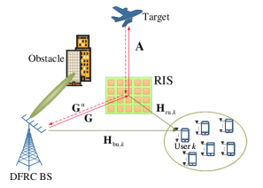
Figure 1: RIS-aided DFRC system with MU-MIMO communication.

where ${\mathbf{\Theta}}={\operatorname{Diag}}\left({\bm{\vartheta}}\right)$ is the phase shift matrix of the RIS and ${\bm{\vartheta}}=\left[{{\vartheta}_{1}},\cdots,{{\vartheta}_{l}},\cdots,{{\vartheta}_{L}}\right]^{\mathrm{T}}$ with $\left|{{\vartheta}_{l}}\right|=1$, $l\in\mathcal{L},\mathcal{L}\triangleq\left\{1,2,\dots,L\right\}$. The vector ${\bf{z}}_{k}\sim\mathcal{CN}{\left(\mathbf{0},\sigma^{2}\mathbf{I}_{M_{k}}\right)}$ denotes the additive white Gaussian noise (AWGN) with variance $\sigma^{2}$. We can define ${\bf{H}}_{k}\triangleq{\bf{H}}_{\mathrm{bu},k}+{\bf{H}}_{\mathrm{ru},k}{\mathbf{\Theta}}^{\rm{H}}{\bf{G}}$, as the representation of the equivalent channel from the BS to CU $k$. Thus, by substituting (1) into (3), ${\bf{y}}_{k}$ is rewritten as

$${\bf{y}}_{k}={\bf{H}}_{k}\sum\limits_{i=1}^{K}{{\bf{B}}_{i}{\bf{d}}_{i}}+{\bf{z}}_{k}.$$ (4)

Let ${\bf{J}}_{k}=\sigma^{2}{\bf{I}}_{M_{k}}+\sum\limits_{i=1,i\neq k}^{K}{\bf{H}}_{k}{\bf{B}}_{i}{\bf{B}}_{i}^{\rm{H}}{\bf{H}}_{k}^{\rm{H}}$ contain the noise and the interference, the achievable sum rate is expressed as

$${R}=\sum\limits_{k=1}^{K}{\log}\left|{\bf{I}}_{M_{k}}+{\bf{H}}_{k}{\bf{B}}_{k}{\bf{B}}_{k}^{\rm{H}}{\bf{H}}_{k}^{\rm{H}}{\bf{J}}_{k}^{-1}\right|.$$ (5)

In urban environments, the presence of surrounding structures often leads to the obstruction of the LoS path, thereby affecting the radar sensing capabilities of the system. When a direct path between the dual-function BS and the target is absent, the dual-function BS transmits a signal, which is subsequently reflected by the RIS. This reflected signal propagates toward the target, and upon its arrival, the target’s echo is received by the BS receiver through the RIS. Consequently, the received echo signal at the BS can be mathematically represented as

$${\bf{y}}_{0}={\bf{G}}^{\rm{H}}{\mathbf{\Theta}}{\bf{A}}{\mathbf{\Theta}}^{\rm{H}}{\bf{G}}{{\bf{x}}}+{\bf{z}}_{0},$$ (6)

where ${\bf{z}}_{0}$ models the AWGN satisfying $\mathcal{CN}\left({\bf{0}},\sigma_{\mathrm{r}}^{2}\mathbf{I}_{N_{\mathrm{r}}}\right)$ at the radar receiver with variance $\sigma_{\mathrm{r}}^{2}$. The matrix ${\bf{A}}\in{\mathbb{C}}^{L\times L}$ is the target response matrix of the RIS. Assuming that RIS can be regarded as a monostatic MIMO radar [26], the point target response matrix can be defined as

$${\bf{A}}={{\bf{a}}}\left(\theta_{0}\right){{{\bf{a}}}^{\mathrm{H}}}\left(\theta_{0}\right),$$ (7)

where $\theta_{0}$ is the direction of the target with respect to (w.r.t.) the RIS.The vector ${\bf{a}}\left(\theta_{0}\right)$ is the steering vector associated with the RIS, defining by

$${\bf{a}}(\theta_{0})=\left[1,\cdots,e^{-j2\pi d\left(L-1\right)\sin\theta_{0}/\lambda}\right]^{\mathrm{T}},$$ (8)

where $d$ and $\lambda$ denote the element spacing and the signal wavelength, respectively.

Following this, we can describe the output received by the radar receiver as

$$r=\mathbf{w}^{\rm{H}}\mathbf{y}_{0}=\eta\mathbf{w}^{\rm{H}}\mathbf{G}^{\mathrm{H}}\mathbf{\Theta A}\bm{\Theta}^{\mathrm{H}}\mathbf{Gx}+\mathbf{w}^{\rm{H}}\mathbf{z}_{0},$$ (9)

where $\eta$ is the channel gain and $\mathbf{w}\in\mathbb{C}^{N_{\rm{t}}\times 1}$ denotes the receive beamforming vector. In order to maximize the radar SNR, minimum variance distortionless response (MVDR) algorithm can be utlized [33], which gives the optimal $\mathbf{w}^{\star}$ as

$$\mathbf{w}^{\star}={\mathop{\operatorname{argmax}}\limits_{\mathbf{w}}}\frac{\left|\mathbf{w}^{\rm{H}}\mathbf{V}\mathbf{x}\right|^{2}}{\mathbf{w}^{\rm{H}}\mathbf{w}}=\beta\mathbf{V}\mathbf{x},$$ (10)

where $\beta$ represents a constant and ${\bf{V}}\triangleq\eta\mathbf{G}^{\mathrm{H}}\mathbf{\Theta A}\bm{\Theta}^{\mathrm{H}}\mathbf{G}$. Thus, the corresponding radar SNR can be computed as

$$\gamma = {\mathbb{E}}\left[\frac{\left|\mathbf{w}^{\rm{H}}\bf{V}\mathbf{x}\right|^{2}}{\sigma_{\mathrm{r}}^{2}\mathbf{w}^{\rm{H}}\mathbf{w}}\right]$$ (11)

$${\stackrel{{\scriptstyle\left(a\right)}}{{=}}} \mathbb{E}\left[\mathbf{x}^{\rm{H}}{\bf{V}}^{\rm{H}}{\bf{V}}\mathbf{x}\right]/\sigma_{\mathrm{r}}^{2}$$

$$\stackrel{{\scriptstyle(b)}}{{=}} \sum_{k=1}^{K}\operatorname{tr}\left({\bf{V}}^{\rm{H}}{\bf{V}}\mathbf{B}_{k}\mathbf{B}_{k}^{\rm{H}}\right)/\sigma_{\mathrm{r}}^{2},$$

where Step (a) corresponds to the determination of the optimal receive beamforming vector ${\bf{w}}^{\star}$, as described in equation (10). Meanwhile, Step (b) results from the mathematical expectation ${{\mathbb{E}}\left[{\bf{xx}}^{\rm{H}}\right]}=\sum_{k=1}^{K}\mathbf{B}_{k}{\bf{B}}_{k}^{\rm{H}}$.

II-B Problem Formulation

In this paper, we aim to jointly optimize the transmit beamforming matrix ${\bf{B}}_{k}$ and the phase shift matrix $\bf{\Theta}$ to maximize the sum rate of the MU-MIMO communication. Specifically, the maximization problem of the MU-MIMO communication sum rate is formulated as

$$\mathop{\max}\limits_{{\left\{\mathbf{B}_{k}\right\}},\mathbf{\Theta}}\quad R$$ (12a)

s.t. $$\mathbf{\gamma}\geq\gamma_{0},$$ (12b)

$$\sum_{k=1}^{K}\operatorname{tr}\left(\mathbf{B}_{k}\mathbf{B}_{k}^{\rm{H}}\right)\leq P_{0},$$ (12c)

$$\left|{{\vartheta}_{l}}\right|=1,l\in\mathcal{L},$$ (12d)

where $\gamma_{0}$ is the required minimum SNR to guarantee the radar sensing performance. The complexity of addressing this optimization problem can be attributed to the intricate coupling that exists between the transmit beamforming matrix ${\bf{B}}_{k}$ and the phase shift matrix $\bf{\Theta}$. Furthermore, the constraints delineated in (12d) exacerbate the challenge.

III The transmit beamforming and RIS phase joint design method

In this section, we commence by reformulating Problem (12) into an equivalent one through the association between data rate and the principle of weighted minimum mean-square error (WMMSE). This approach allows us to lay the foundation for subsequent optimization steps. Subsequently, we utilize the AO method to address the reformulated problem, acknowledging the coupling among optimization variables. The method facilitates the decomposition of the intricate problem into two noticeable subproblems, each dedicated to optimizing specific variables, thereby enhancing the tractability of the overall optimization procedure. To address the optimization problem associated with transmit beamforming matrix, we implement a penalty-based algorithm. Concurrently, we employ the MM algorithm to reformulate the quartic non-convex constraint and subsequently utilize the SDR method for phase shift matrix optimization. Via this approach, we can address the coupling between ${\bf{B}}_{k}$ and the phase shift matrix $\bf{\Theta}$ and handle the non-convex constraints effectively, ultimately optimizing the system performance.

III-A Reformulation of the Original Problem

Without loss of generality, we consider an arbitrary CU $k$ and show how to reformulate the corresponding problem. We assume a linear decoding matrix $\mathbf{U}_{k}\in\mathbb{C}^{M_{k}\times D_{k}}$, which allows us to compute the estimated signal vector ${{{\bf{\hat{d}}}}_{k}}$ for CU $k$ as

$${{{\bf{\hat{d}}}}_{k}}={\bf{U}}_{k}^{\rm{H}}{{\bf{y}}_{k}},\forall k.$$ (13)

Then, we can calculate the mean-square error (MSE) matrix for the $k$-th CU as

$$\mathbf{E}_{k} = \mathbb{E}\left[\left({\bf{\hat{d}}}_{k}-{\bf{d}}_{k}\right){\left({\bf{\hat{d}}}_{k}-{\bf{d}}_{k}\right)}^{\rm{H}}\right]$$ (14)

$$= {\bf{U}}_{k}^{\rm{H}}{\bf{H}}_{k}\left(\sum\limits_{i=1}^{K}{{\bf{B}}_{i}}{\bf{B}}_{i}^{\rm{H}}\right){\bf{H}}_{k}^{\rm{H}}{\bf{U}}_{k}-{\bf{U}}_{k}^{\rm{H}}{\bf{H}}_{k}{{\bf{B}}_{k}}$$

$$-{\bf{B}}_{k}^{\rm{H}}{\bf{H}}_{k}^{\rm{H}}{\bf{U}}_{k}+\sigma^{2}{\bf{U}}_{k}^{\rm{H}}{\bf{U}}_{k}+{\bf{I}}_{D_{k}}.$$

Subsequently, the expression for $R$ in (5) can be transformed as

$${E}=\sum_{k=1}^{K}\left(\log\left|\mathbf{W}_{k}\right|-\operatorname{tr}\left(\mathbf{W}_{k}\mathbf{E}_{k}\right)+D_{k}\right),$$ (15)

where ${\bf{W}}_{k}\in\mathbb{C}^{{D_{k}\times D_{k}}}$ represents the auxiliary matrix for the $k$-th CU and $D_{k}$ is the constant term.

Hence, by ignoring the constant term of (15), we can reformulate Problem (12) as follows[34]:

$$\mathop{\min}\limits_{\left\{\mathbf{B}_{k},{\bf{W}}_{k},{\bf{U}}_{k}\right\},\mathbf{\Theta}}\quad \sum_{k=1}^{K}\left(\operatorname{tr}\left(\mathbf{W}_{k}\mathbf{E}_{k}\right)-\log\left|\mathbf{W}_{k}\right|\right)$$ (16a)

s.t. $$(\ref{SNR}),(\ref{Power}),(\ref{phase}),$$ (16b)

due to the challenges posed by the coupled variables in Problem (16), attaining the optimal solution is an awkward task. In order to address this issue, the most widely used and practical approach is to employ an AO mechanism. Specifically, we optimize a specific group of variables while maintaining the others fixed to minimize the objective function (16a). In Problem (16), it is discernible that matrices $\mathbf{U}_{k}$ and ${\bf{W}}_{k}$ are exclusively associated with the objective function. Consequently, we commence by setting the first-order derivative of ${E}$ w.r.t. $\mathbf{U}_{k}$ to zero while maintaining the other three variables fixed. This approach enables us to deduce the optimal solution for $\mathbf{U}_{k}$ as [35, 36]

$$\mathbf{U}_{k}^{\mathrm{opt}}=\left({\bf{H}}_{k}\sum_{i=1}^{K}\mathbf{B}_{i}\mathbf{B}_{i}^{\rm{H}}{\bf{H}}_{k}^{\rm{H}}+\sigma^{2}\mathbf{I}_{M_{k}}\right)^{-1}{\bf{H}}_{k}{\mathbf{B}_{k}}.$$ (17)

Similarly, upon fixing the values for the other three matrices except $\mathbf{W}_{k}$, we can deduce the optimal solution for matrix $\mathbf{W}_{k}$ as

$$\mathbf{W}_{k}^{\mathrm{opt}}=\mathbf{E}_{k}^{-1}.$$ (18)

III-B Optimize the Transmit Beamforming Matrix $\mathbf{B}_{k}$

Our primary focus is on optimizing the transmit beamforming matrix $\left\{\mathbf{B}_{k}\right\}$, while keeping $\bm{\Theta}$, $\left\{{\mathbf{W}}_{k}\right\}$, and $\left\{{\mathbf{U}}_{k}\right\}$ fixed. First of all, we substitute $\mathbf{E}_{k}$ into (15) and remove the constant terms, then the transmit beamforming matrix optimization problem is formulated as

$$\mathop{\min}\limits_{\left\{\mathbf{B}_{k}\right\}}\quad -\sum_{k=1}^{K}\operatorname{tr}\left(\mathbf{W}_{k}\mathbf{U}_{k}^{\rm{H}}\mathbf{H}_{k}\mathbf{B}_{k}\right)$$

$$+\sum_{k=1}^{K}\operatorname{tr}\left(\mathbf{B}_{k}^{\rm{H}}\sum_{m=1}^{K}\mathbf{H}_{m}^{\rm{H}}\mathbf{U}_{m}\mathbf{W}_{m}\mathbf{U}_{m}^{\rm{H}}\mathbf{H}_{m}\mathbf{B}_{k}\right)$$

$$-\sum_{k=1}^{K}\operatorname{tr}\left(\mathbf{W}_{k}\mathbf{B}_{k}^{\rm{H}}\mathbf{H}_{k}^{\rm{H}}\mathbf{U}_{k}\right)$$ (19a)

s.t. $$(\ref{SNR}),(\ref{Power}).$$ (19b)

Problem (19) poses a substantial challenge for resolution, primarily attributed to the non-convex constraints (12b). To address the non-convex constraints, a penalty-based algorithm is utilized[37]. Specifically, we first introduce auxiliary variables $\mathbf{X}_{k},\mathbf{Y}_{k}$ and define $\mathbf{X}_{k}=\mathbf{B}_{k},\mathbf{Y}_{k}=\mathbf{V}\mathbf{B}_{k}$. Then Problem (19) can be rewritten as

$$\mathop{\min}\limits_{\left\{\mathbf{B}_{k},\mathbf{X}_{k},\mathbf{Y}_{k}\right\}} -\sum_{k=1}^{K}\operatorname{tr}\left(\mathbf{W}_{k}\mathbf{U}_{k}^{\rm{H}}\mathbf{H}_{k}\mathbf{B}_{k}\right)$$

$$+\sum_{k=1}^{K}\operatorname{tr}\left(\mathbf{B}_{k}^{\rm{H}}\sum_{m=1}^{K}\mathbf{H}_{m}^{\rm{H}}\mathbf{U}_{m}\mathbf{W}_{m}\mathbf{U}_{m}^{\rm{H}}\mathbf{H}_{m}\mathbf{B}_{k}\right)$$

$$-\sum_{k=1}^{K}\operatorname{tr}\left(\mathbf{W}_{k}\mathbf{B}_{k}^{\rm{H}}\mathbf{H}_{k}^{\rm{H}}\mathbf{U}_{k}\right)$$ (20a)

s.t. $$\quad\sum_{k=1}^{K}\operatorname{tr}\left(\mathbf{X}_{k}\mathbf{X}_{k}^{\rm{H}}\right)\leq P_{0},$$ (20b)

$$\quad\sum_{k=1}^{K}\operatorname{tr}\left(\mathbf{Y}_{k}\mathbf{Y}_{k}^{\rm{H}}\right)\geq\sigma_{\mathrm{r}}^{2}\gamma_{0},$$ (20c)

$$\quad\mathbf{X}_{k}=\mathbf{B}_{k},\mathbf{Y}_{k}=\mathbf{V}\mathbf{B}_{k},\quad k=1,\cdots,K.$$ (20d)

Subsequently, we incorporate (20d) as penalty terms which are introduced into (20a), resulting in the following penalty-based optimization problem

$$\mathop{\min}\limits_{{\left\{\mathbf{B}_{k},\mathbf{X}_{k},\mathbf{Y}_{k}\right\}}} -\sum_{k=1}^{K}\operatorname{tr}\left(\mathbf{W}_{k}\mathbf{U}_{k}^{\rm{H}}\mathbf{H}_{k}\mathbf{B}_{k}\right)-\sum_{k=1}^{K}\operatorname{tr}\left(\mathbf{W}_{k}\mathbf{B}_{k}^{\rm{H}}\mathbf{H}_{k}^{\rm{H}}\mathbf{U}_{k}\right)$$

$$+\sum_{k=1}^{K}\operatorname{tr}\left(\mathbf{B}_{k}^{\rm{H}}\sum_{m=1}^{K}\mathbf{H}_{m}^{\rm{H}}\mathbf{U}_{m}\mathbf{W}_{m}\mathbf{U}_{m}^{\rm{H}}\mathbf{H}_{m}\mathbf{B}_{k}\right)$$

$$+\frac{1}{2\rho^{\left[t\right]}}\left(\sum_{k=1}^{K}\|{\mathbf{X}_{k}}-\mathbf{B}_{k}\|_{F}^{2}+\sum_{k=1}^{K}\|{\mathbf{Y}_{k}}-\mathbf{V}\mathbf{B}_{k}\|_{F}^{2}\right)$$ (21a)

s.t. $$(\ref{X_Con}),(\ref{Y_Con}),$$ (21b)

where $\rho^{\left[t\right]}\left(\rho^{\left[t\right]}>0\right)$ is the penalty coefficient associated with constraint (20d) in the $t$-th iteration. During the whole iteration, We aim to encourage the optimization process to satisfy (20d) closely as possible while maintaining the goal of minimizing the objective function. To attain this objective, in the outer iteration, we decrease the penalty coefficient’s value, driving the coefficient $\frac{1}{2\rho^{\left[t\right]}}$ toward infinity. Ultimately, through the optimization process, the equality constraint is achieved. Essentially, the method offers a way to strike a balance in optimization, aligning it with the dual goals of achieving the original objective function and complying with the equality constraints.

In the inner layer of the penalty-based algorithm, the penalty coefficient $\rho^{\left[t\right]}$ remains constant. However, the problem concerning these three optimization variables is still non-convex. Fortunately, it can be decomposed into two subproblems: one for optimizing the beamforming matrix and the other for optimizing the auxiliary matrix, respectively. These two subproblems are alternately solved until convergence.

In the following sections, we provide a comprehensive exposition of the procedures involved in both the outer and inner optimization layers within the penalty-based algorithm.

III-B1 Outer Layer Update

In the outer layer, the penalty coefficient $\rho^{\left[t\right]}$ in the $t$-th iteration can be updated as

$$\rho^{\left[t\right]}=c\rho^{\left[t-1\right]},$$ (22)

where $c\left(0<c<1\right)$ represents the updated step size. Subsequently, without loss of generality, we take the $t$-th outer layer update as an example to specifically introduce the inner layer optimization.

III-B2 Inner Layer Optimization

III-B2a With fixed $\left\{\mathbf{X}_{k},\mathbf{Y}_{k}\right\}$, optimize $\left\{\mathbf{B}_{k}\right\}$

For given auxiliary variables $\left\{\mathbf{X}_{k},\mathbf{Y}_{k}\right\}$, the subproblem associated with the optimization of transmit beamforming can be formulated as

$$\begin{split}\mathop{\min}\limits_{\left\{{\mathbf{B}_{k}}\right\}}&-\sum_{k=1}^{K}\operatorname{tr}\left(\mathbf{W}_{k}\mathbf{U}_{k}^{\rm{H}}\mathbf{H}_{k}\mathbf{B}_{k}\right)-\sum_{k=1}^{K}\operatorname{tr}\left(\mathbf{W}_{k}\mathbf{B}_{k}^{\rm{H}}\mathbf{H}_{k}^{\rm{H}}\mathbf{U}_{k}\right)\\ &+\sum_{k=1}^{K}\operatorname{tr}\left(\mathbf{B}_{k}^{\rm{H}}\sum_{m=1}^{K}\mathbf{H}_{m}^{\rm{H}}\mathbf{U}_{m}\mathbf{W}_{m}\mathbf{U}_{m}^{\rm{H}}\mathbf{H}_{m}\mathbf{B}_{k}\right)\\ &+\frac{1}{2\rho^{(t)}}\left(\sum_{k=1}^{K}\|{\mathbf{X}_{k}}-\mathbf{B}_{k}\|_{F}^{2}+\sum_{k=1}^{K}\|{\mathbf{Y}_{k}}-\mathbf{V}\mathbf{B}_{k}\|_{F}^{2}\right).\end{split}$$ (23)

Given that Problem (23) is an unconstrained convex quadratic minimization problem, we can find the optimal solution by utilizing the first-order optimality conditions. Specifically, setting the first-order derivative of (23) w.r.t. $\mathbf{B}_{k}$ to zero, we obtain the optimal solution for $\mathbf{B}_{k}$ as

$$\begin{split}\mathbf{B}_{k}^{\mathrm{opt}}&=\left(2\sum_{m=1}^{K}\mathbf{H}_{m}^{\rm{H}}\mathbf{U}_{m}\mathbf{W}_{m}\mathbf{U}_{m}^{\rm{H}}\mathbf{H}_{m}+\frac{1}{\rho^{(t)}}\left(\mathbf{I}_{N_{\rm{t}}}+\mathbf{V}^{\rm{H}}\mathbf{V}\right)\right)^{-1}\\ &\quad\times\left(\frac{1}{\rho^{(t)}}\left(\mathbf{X}_{k}+\mathbf{V}^{\rm{H}}\mathbf{Y}_{k}\right)+2\mathbf{H}_{k}^{\rm{H}}\mathbf{U}_{k}\mathbf{W}_{k}\right).\end{split}$$ (24)

III-B2b With fixed $\left\{\mathbf{B}_{k}\right\}$, optimize $\left\{\mathbf{X}_{k},\mathbf{Y}_{k}\right\}$

For given transmit beamforming matrices $\left\{\mathbf{B}_{k}\right\}$, we can get the following optimization subproblem in which only items related to $\left\{\mathbf{X}_{k}\right\}$ and $\left\{\mathbf{Y}_{k}\right\}$ are kept

$$\mathop{\min}\limits_{\left\{{\mathbf{X}_{k},\mathbf{Y}_{k}}\right\}}\quad \frac{1}{2\rho^{(t)}}\left(\sum_{k=1}^{K}\|{\mathbf{X}_{k}}-\mathbf{B}_{k}\|_{F}^{2}+\sum_{k=1}^{K}\|{\mathbf{Y}_{k}}-\mathbf{V}\mathbf{B}_{k}\|_{F}^{2}\right)$$ (25a)

s.t. $$(\ref{X_Con}),(\ref{Y_Con}).$$ (25b)

Since optimization variables w.r.t. different blocks $\left\{\mathbf{X}_{k}\right\}$ and $\left\{\mathbf{Y}_{k}\right\}$ are separated in both the objective function and constraints. Therefore, Problem (25) can be divided into two separated subproblems, which can be solved in a parallel manner as follows.

Algorithm 1 Bisection search method to solve Problem (26).

1:Initialize the accuracy $\eta,$ the bounds $\mu_{{\rm{lb}}}$ and $\mu_{{\rm{ub}}}$;

2:If $h(0)\geq\sigma_{\mathrm{r}}^{2}\gamma_{0}$ holds, the auxiliary variable $\mathbf{Y}_{k}$ is given by $\mathbf{Y}_{k}^{\mathrm{opt}}=\mathbf{Y}_{k}\left(0\right),\forall k$ and terminate; Othersize, go to Step 3;

3:Calculate $\mu=\left(\mu_{{\rm{lb}}}+\mu_{{\rm{ub}}}\right)/2$;

4:If $h({\mu})\geq\sigma_{\mathrm{r}}^{2}\gamma_{0}$, set ${\mu_{\rm{ub}}}={\mu}$. Otherwise, set ${\mu_{\rm{lb}}}={\mu}$;

5:If $\left|{\mu_{\rm{lb}}-\mu_{\rm{ub}}}\right|\leq\eta$, terminate. Otherwise, go to Step 2.

First, our focus turns to the optimization problem associated with $\left\{\mathbf{Y}_{k}\right\}$, which is expressed as follows:

$$\mathop{\min}\limits_{\left\{{\mathbf{Y}_{k}}\right\}}\quad \sum_{k=1}^{K}\|{\mathbf{Y}_{k}}-\mathbf{V}\mathbf{B}_{k}\|_{F}^{2}$$ (26a)

s.t. $$(\ref{Y_Con}).$$ (26b)

It has been noted that Problem (26) constitutes a quadratic constraint quadratic programming (QCQP) problem. To find the optimal solution for Problem (26), one can solve its corresponding dual problem[38]. We formulate the Lagrangian function of Problem (26) associated with Lagrange multiplier $\mu$ ($\mu\geq 0$) as

$$\mathcal{L}_{1}\left(\mathbf{Y}_{k},\mu\right) = \sum_{k=1}^{K}(1-\mu)\|{\mathbf{Y}_{k}}\|_{F}^{2}-\sum_{k=1}^{K}2\operatorname{Re}\left(\mathbf{B}_{k}^{\rm{H}}\mathbf{V}^{\rm{H}}{\mathbf{Y}_{k}}\right)$$ (27)

$$+ \sum_{k=1}^{K}\|{\mathbf{V}\mathbf{B}_{k}}\|_{F}^{2}+\mu\sigma_{{\rm{r}}}^{2}\gamma_{0}.$$

Define $f_{1}\left(\mu\right)=\min_{\mathbf{Y}_{k}}\mathcal{L}_{1}\left(\mathbf{Y}_{k},\mu\right)$ as the dual function of Problem (26). Besides, to ensure the boundedness of the dual function $f_{1}(\mu)$, we can deduce that $0\leq\mu<1$. Once we set $\mu>1$ meaning $1-\mu$, which is the coefficient in front of the $\|{\mathbf{Y}_{k}}\|_{F}^{2}$ less than zero. In that case, if we set ${\mathbf{Y}_{k}}=\varrho\mathbf{I}$ and let $\varrho$ be positive infinity, the $f_{1}\left(\mu\right)$ is unbounded. Similar considerations apply for $\mu=1.$ Accordingly, the Lagrange multiplier $\mu$ is constrained within the range of $0\leq\mu<1.$

By leveraging the first-order optimality conditions, we can determine the best solution for $f_{1}\left(\mu\right)$ as

$$\mathbf{Y}_{k}^{\mathrm{opt}}\left(\mu\right)=\frac{\mathbf{V}\mathbf{B}_{k}}{1-\mu},\quad k=1,\cdots,K.$$ (28)

Then, we define

$$h\left(\mu\right) \triangleq \sum_{k=1}^{K}\operatorname{tr}\left(\mathbf{Y}_{k}\left(\mu\right)\mathbf{Y}_{k}^{\rm{H}}\left(\mu\right)\right)$$ (29)

$$= \operatorname{tr}\left(\left(1-\mu\right)^{-2}\mathbf{\Gamma}\right)$$

$$= \sum_{i=1}^{N_{\rm{t}}}\frac{[\mathbf{\Gamma}]_{i,i}}{\left(1-\mu\right)^{2}},$$

where $\mathbf{\Gamma}=\sum_{k=1}^{K}\mathbf{V}\mathbf{B}_{k}\mathbf{B}_{k}^{\rm{H}}\mathbf{V}^{\rm{H}}$ and $[\mathbf{\Gamma}]_{i,i}$ denotes the $i$-th diagonal element of matrix $\mathbf{\Gamma}$. It is easy to confirm that $h\left(\mu\right)$ exhibits a strictly increasing trend for $0\leq\mu<1$. If $h\left(0\right)>\sigma^{2}_{\mathrm{r}}\gamma_{0}$, then the corresponding optimal dual variable $\mu^{\mathrm{opt}}=0$. Otherwise, according to the complementary condition of $\mu\left(\sigma_{\mathrm{r}}^{2}\gamma_{0}-h\left(\mu\right)\right)=0,$ we need to find a positive $\mu$ according to the following equation:

$$h\left(\mu\right)=\sigma_{\mathrm{r}}^{2}\gamma_{0}.$$ (30)

By exploiting the monotonic property of $h\left(\mu\right)$, the solution $\mu^{\mathrm{opt}}$ can be easily obtained using a straightforward bisection search method [23], ranging from $0$ to $1$. The overall algorithm to solve Problem (26) is summarized in Algorithm 1.

Second, the subproblem associated with $\left\{\mathbf{X}_{k}\right\}$ is given by

$$\mathop{\min}\limits_{\left\{\mathbf{X}_{k}\right\}}\quad \sum_{k=1}^{K}\|{\mathbf{X}_{k}}-\mathbf{B}_{k}\|_{F}^{2}$$ (31a)

s.t. $$(\ref{X_Con}).$$ (31b)

Fortunately, Problem (31) is a convex problem which can be solved by solving its dual problem. We formulate the Lagrangian function of Problem (31) associated with Lagrange multiplier $\tau\left(\tau\geq 0\right)$ as

$$\mathcal{L}_{2}\left(\mathbf{X}_{k},\tau\right)=\sum_{k=1}^{K}\|{\mathbf{X}_{k}}-\mathbf{B}_{k}\|^{2}_{F}+\tau\left(\sum_{k=1}^{K}\operatorname{tr}\left(\mathbf{X}_{k}\mathbf{X}_{k}^{\rm{H}}\right)-P_{0}\right).$$ (32)

Define $f_{2}\left(\tau\right)=\min_{\mathbf{X}_{k}}\mathcal{L}_{2}\left(\mathbf{X}_{k},\tau\right)$ as the dual function of Problem (31).

By leveraging the first-order optimality conditions, we can determine the best solution for $f_{2}\left(\tau\right)$ as

$$\mathbf{X}_{k}^{{\rm{opt}}}\left(\tau\right)=\frac{\mathbf{B}_{k}}{1+\tau},\quad k=1\cdots,K.$$ (33)

Similarly, we define

$$g\left(\tau\right) \triangleq \sum_{k=1}^{K}\operatorname{tr}\left(\mathbf{X}_{k}\left(\tau\right)\mathbf{X}_{k}^{\rm{H}}\left(\tau\right)\right)$$ (34)

$$= \operatorname{tr}\left(\left(1+\tau\right)^{-2}\mathbf{M}\right)$$

$$= \sum_{i=1}^{D_{k}}\frac{[\mathbf{M}]_{i,i}}{\left(1+\tau\right)^{2}},$$ (35)

where $\mathbf{M}=\sum_{k=1}^{K}\mathbf{B}_{k}^{\rm{H}}\mathbf{B}_{k}$ and $[\mathbf{M}]_{i,i}$ denote the $i$-th diagonal element of matrix $\mathbf{M}$. It can be easily confirmed that $g(\tau)$ exhibits a monotonically decreasing tend for $\tau\geq 0$. Hence, if $g(0)\leq P_{0}$, the corresponding optimal dual variable $\tau^{\mathrm{opt}}=0$. Otherwise, according to the complementary condition:

$$\tau\left(\sum_{k=1}^{K}\operatorname{tr}\left(\mathbf{X}_{k}\left(\tau\right)\mathbf{X}_{k}^{\rm{H}}\left(\tau\right)\right)-P_{0}\right)=0,$$ (36)

we need to find a positive $\tau$ by using the bisection based search method according to the following equation:

$$g\left(\tau\right)=\sum_{i=1}^{D_{k}}\frac{[\mathbf{M}]_{i,i}}{\left(1+\tau_{{\rm{ub}}}\right)^{2}}=P_{0}.$$ (37)

To apply the bisection search method, we have to find the upper bound of $\tau$, which is given by

$$\tau<\sqrt{\frac{\sum_{i=1}^{D_{k}}[\mathbf{M}]_{i,i}}{P_{0}}}\triangleq\tau_{{\rm{ub}}}.$$ (38)

This can be proved as follows:

$$g\left(\tau_{{\rm{ub}}}\right)=\sum_{i=1}^{D_{k}}\frac{[\mathbf{M}]_{i,i}}{\left(1+\tau_{{\rm{ub}}}\right)^{2}}<\frac{\sum_{i=1}^{D_{k}}[\mathbf{M}]_{i,i}}{\tau_{{\rm{ub}}}^{2}}=P_{0}.$$ (39)

Algorithm 2 Penalty-based algorithm for solving Problem (19).

1:Initialize $\left\{\mathbf{B}_{k}^{\left[0\right]}\right\}=\left\{\mathbf{B}_{k}^{\left(\mathrm{n}\right)}\right\}$ ,$\left\{\mathbf{X}_{k}^{\left[0\right]}\right\}=\left\{\mathbf{B}_{k}^{\left(\mathrm{n}\right)}\right\}$, $\left\{\mathbf{Y}_{k}^{\left[0\right]}\right\}=\left\{\mathbf{V}\mathbf{B}_{k}^{\left(\mathrm{n}\right)}\right\}$, $t=0$, the penalty coefficient $\rho^{0}$, step size $c$ , tolerance of accuracy $\xi$ and $\epsilon$.

2:while the fractional increase of (19a) is larger than $\epsilon$ or penalty terms larger than $\xi$ do

3:     Update $\mathbf{B}_{k}^{[t+1]}$ by using (24);

4:     Update $\mathbf{Y}_{k}^{[t+1]}$ via Algorithm 1;

5:     Update $\mathbf{X}_{k}^{[t+1]}$ by solving Problem (31);

6:     Set $\rho^{[t+1]}=c\rho^{[t]},t\leftarrow t+1$.

7:end while

8:$\left\{\mathbf{B}_{k}^{\left(n+1\right)}\right\}=\left\{\mathbf{B}_{k}^{\left[t\right]}\right\}$.

III-C Optimize the Phase Shift Matrix $\bf{\Theta}$

In the following, our primary focus lies in optimizing matrix $\bm{\Theta}$ while keeping $\left\{{\bf{B}}_{k}\right\}$, $\left\{{\mathbf{W}}_{k}\right\}$, and $\left\{{\mathbf{U}}_{k}\right\}$ fixed. We first substitute $\mathbf{E}_{k}$ into (15) and eliminate the constant terms, we can formulate the optimization problem for phase shift as follows:

$$\mathop{\min}\limits_{{\bm{\Theta}}}\quad -\sum_{k=1}^{K}\operatorname{tr}\left(\mathbf{W}_{k}\mathbf{U}_{k}^{\rm{H}}\mathbf{H}_{k}\mathbf{B}_{k}\right)$$

$$+\sum_{k=1}^{K}\operatorname{tr}\left(\mathbf{W}_{k}\mathbf{U}_{k}^{\rm{H}}\mathbf{H}_{k}\sum\limits_{i=1}^{K}{{\bf{B}}_{i}}{\bf{B}}_{i}^{\rm{H}}\mathbf{H}_{k}^{\rm{H}}\mathbf{U}_{k}\right)$$

$$-\sum_{k=1}^{K}\operatorname{tr}\left(\mathbf{W}_{k}\mathbf{B}_{k}^{\rm{H}}\mathbf{H}_{k}^{\rm{H}}\mathbf{U}_{k}\right)$$ (40a)

s.t. $$(\ref{SNR}),(\ref{phase}).$$ (40b)

First, let us define ${\bf{B}}=\sum_{k=1}^{K}{\bf{B}}_{k}{\bf{B}}_{k}^{\rm{H}}$, by substituting ${\bf{H}}_{k}={\bf{H}}_{{\rm{bu}},k}+{\bf{H}}_{{\rm{ru}},k}{\mathbf{\Theta}}^{\rm{H}}{\bf{G}}$ into $\mathbf{W}_{k}\mathbf{U}_{k}^{\rm{H}}\mathbf{H}_{k}\sum\limits_{i=1}^{K}{{\bf{B}}_{i}}{\bf{B}}_{i}^{\rm{H}}\mathbf{H}_{k}^{\rm{H}}\mathbf{U}_{k}$, we have

$$\mathbf{W}_{k}\mathbf{U}_{k}^{\rm{H}}\mathbf{H}_{k}\sum\limits_{i=1}^{K}{{\bf{B}}_{i}} {\bf{B}}_{i}^{\rm{H}}\mathbf{H}_{k}^{\rm{H}}\mathbf{U}_{k}=\mathbf{W}_{k}\mathbf{U}_{k}^{\rm{H}}\mathbf{H}_{{\rm{bu}},k}{{\bf{B}}}\mathbf{H}_{{\rm{bu}},k}^{\rm{H}}\mathbf{U}_{k}$$ (41)

$$\qquad\qquad\qquad+ \mathbf{W}_{k}\mathbf{U}_{k}^{\mathrm{H}}\mathbf{H}_{{\rm{ru}},k}\mathbf{\Theta}^{\mathrm{H}}\mathbf{G}\mathbf{BG}^{\mathrm{H}}\mathbf{\Theta}\mathbf{H}_{{\rm{ru}},k}^{\mathrm{H}}\mathbf{U}_{k}$$

$$+ \mathbf{W}_{k}\mathbf{U}_{k}^{\rm{H}}\mathbf{H}_{{\rm{ru}},k}{\mathbf{\Theta}}^{\rm{H}}{{\bf{G}}}{{\bf{B}}}\mathbf{H}_{{\rm{bu}},k}^{\rm{H}}\mathbf{U}_{k}\qquad$$

$$+ \mathbf{W}_{k}\mathbf{U}_{k}^{\rm{H}}\mathbf{H}_{{\rm{bu}},k}{{\bf{B}}}{{\bf{G}}}^{\rm{H}}{\mathbf{\Theta}}\mathbf{H}_{{\rm{ru}},k}^{\rm{H}}\mathbf{U}_{k}\qquad\qquad\qquad$$

and

$$\mathbf{W}_{k}\mathbf{U}_{k}^{\rm{H}}\mathbf{H}_{k}\mathbf{B}_{k}=\mathbf{W}_{k}\mathbf{U}_{k}^{\rm{H}}\mathbf{H}_{{\rm{ru}},k}{\mathbf{\Theta}}^{\rm{H}}{{\bf{G}}}\mathbf{B}_{k}+\mathbf{W}_{k}\mathbf{U}_{k}^{\rm{H}}\mathbf{H}_{{\rm{bu}},k}\mathbf{B}_{k}.$$ (42)

Then, by defining $\mathbf{C}_{k}=\mathbf{H}_{{\rm{ru}},k}^{\rm{H}}\mathbf{U}_{k}\mathbf{W}_{k}\mathbf{U}_{k}^{\rm{H}}\mathbf{H}_{{\rm{ru}},k}$, $\mathbf{D}={{\bf{G}}}{{\bf{B}}}{{\bf{G}}}^{\rm{H}}$ and $\mathbf{E}_{k}^{\rm{H}}={{\bf{G}}}{{\bf{B}}}\mathbf{H}_{{\rm{bu}},k}^{\rm{H}}\mathbf{U}_{k}\mathbf{W}_{k}\mathbf{U}_{k}^{\rm{H}}\mathbf{H}_{{\rm{ru}},k}$, and using (41), we can obtain

$$\operatorname{tr}(\mathbf{W}_{k}\mathbf{U}_{k}^{\rm{H}}\mathbf{H}_{k}\sum\limits_{i=1}^{K}{{\bf{B}}_{i}}{\bf{B}}_{i}^{\rm{H}}\mathbf{H}_{k}^{\rm{H}}\mathbf{U}_{k})=\operatorname{tr}\left(\mathbf{C}_{k}{\mathbf{\Theta}}^{\rm{H}}\mathbf{D}{\mathbf{\Theta}}\right)+\operatorname{tr}\left(\mathbf{E}_{k}{\mathbf{\Theta}}\right)$$ (43)

$$+\operatorname{tr}\left(\mathbf{E}_{k}^{\rm{H}}{\mathbf{\Theta}}^{\rm{H}}\right)+\underbrace{\operatorname{tr}(\mathbf{W}_{k}\mathbf{U}_{k}^{\rm{H}}\mathbf{H}_{{\rm{bu}},k}{\sum_{k=i}^{K}{\bf{B}}_{i}{\bf{B}}_{i}^{\rm{H}}}\mathbf{H}_{{\rm{bu}},k}^{\rm{H}}\mathbf{U}_{k})}_{\rm{const}_{1}},$$

where ${\rm{const}_{1}}$ is a constant term that does not depend on $\mathbf{\Theta}$.

Similarly, define $\mathbf{F}_{k}^{\rm{H}}=\mathbf{G}\mathbf{B}_{k}\mathbf{W}_{k}\mathbf{U}_{k}^{\rm{H}}\mathbf{H}_{{\rm{ru}},k}$, we can obtain

$$\operatorname{tr}\left(\mathbf{W}_{k}\mathbf{U}_{k}^{\rm{H}}\mathbf{H}_{k}\mathbf{B}_{k}\right)=\operatorname{tr}\left(\mathbf{\Theta}^{\rm{H}}\mathbf{F}_{k}^{\rm{H}}\right)+\underbrace{\operatorname{tr}\left(\mathbf{W}_{k}\mathbf{U}_{k}^{\rm{H}}\mathbf{H}_{{\rm{bu}},k}\mathbf{B}_{k}\right)}_{\rm{const}_{2}},$$ (44)

where ${\rm{const}_{2}}$ is a constant term that does not depend on $\mathbf{\Theta}$.

From (43) and (44), the objective function (40a) can be derived as:

$$\operatorname{tr}\left(\mathbf{C}\mathbf{\Theta}^{\rm{H}}\mathbf{D}\mathbf{\Theta}\right)+\operatorname{tr}\left(\mathbf{Z}\mathbf{\Theta}^{\rm{H}}\right)+\operatorname{tr}\left(\mathbf{Z}^{\rm{H}}\mathbf{\Theta}\right),$$ (45)

where $\mathbf{C}=\sum_{k=1}^{K}\mathbf{C}_{k}$ and $\mathbf{Z}=\sum_{k=1}^{K}\left(\mathbf{E}_{k}^{\rm{H}}-\mathbf{F}_{k}^{\rm{H}}\right)$. Furthermore, using ${\bm{\vartheta}}$, we arrive at [39, Eq. (1.10.6)]

$$\operatorname{tr}\left(\mathbf{C}\mathbf{\Theta}^{\rm{H}}\mathbf{D}\mathbf{\Theta}\right)={\bm{\vartheta}}^{\mathrm{H}}\mathbf{\Xi}{\bm{\vartheta}},$$ (46)

where $\mathbf{\Xi}=\mathbf{D}\odot\mathbf{C}^{\mathrm{T}}$.

Let $\mathbf{z}$ be the collection of diagonal elements of matrix $\mathbf{Z}$, given by $\mathbf{z}=\operatorname{diag}{\left(\mathbf{Z}\right)}$. Then, we have

$$\operatorname{tr}(\mathbf{\Theta}\mathbf{Z}^{\rm{H}})=\mathbf{z}^{\mathrm{H}}{\bm{\vartheta}}.$$ (47)

Hence, the objective function of Problem (40) can be rewritten as ${\bm{\vartheta}}^{\mathrm{H}}\mathbf{\Xi}{\bm{\vartheta}}+\mathbf{z}^{\mathrm{H}}{\bm{\vartheta}}+{\bm{\vartheta}}^{\mathrm{H}}\mathbf{z}.$

In the following, we reformulate the left-hand-side (LHS) of the radar SNR constraint (12b) in a more tractable way. According to the equation $\operatorname{tr}\left(\mathbf{ABCD}\right)=\left(\operatorname{vec}\left(\mathbf{D}^{\rm{T}}\right)\right)^{\rm{T}}(\mathbf{C}^{\rm{T}}\otimes\mathbf{A})\operatorname{vec}\left({\mathbf{B}}\right)$, we have

$$\operatorname{tr}\left({\bf{V}}^{\rm{H}}{\bf{V}}\mathbf{B}_{k}\mathbf{B}_{k}^{\rm{H}}\right)= (\operatorname{vec}((\operatorname{\mathbf{\Theta}\mathbf{A}\mathbf{\Theta}^{\rm{H}}})^{\rm{T}}))^{\rm{T}}((\mathbf{G}^{*}\mathbf{G}^{\rm{T}})$$ (48)

$$\otimes\left(\mathbf{G}\mathbf{B}_{k}\mathbf{B}_{k}^{\rm{H}}\mathbf{G}^{\rm{H}}\right))\operatorname{vec}\left(\mathbf{\Theta}\mathbf{A}\mathbf{\Theta}^{\rm{H}}\right).$$

As $\mathbf{A}$ is a Hermitian matrix, after some further manipulations, we obtain

$$(\operatorname{vec}((\operatorname{\mathbf{\Theta}\mathbf{A}\mathbf{\Theta}^{\rm{H}}})^{\rm{T}}))^{\rm{T}}=(\operatorname{vec}(\operatorname{\mathbf{\Theta}\mathbf{A}\mathbf{\Theta}^{\rm{H}}}))^{\rm{H}}=\operatorname{Diag}\left({\operatorname{vec}\left(\mathbf{A}\right)}\right)\hat{\bm{\vartheta}},$$ (49)

where $\hat{\bm{\vartheta}}$ is a vector of diagonal elements of the matrix $\left(\mathbf{\Theta}^{*}\otimes\mathbf{\Theta}\right)$. Thus, (48) can be expressed as

$$\hat{\bm{\vartheta}}^{\rm{H}}\mathbf{Q}_{k}\hat{\bm{\vartheta}},$$ (50)

where

$$\mathbf{Q}_{k} =\left(\operatorname{Diag}\left({\operatorname{vec}{\left(\mathbf{A}\right)}}\right)\right)^{\rm{H}}((\mathbf{G}^{*}\mathbf{G}^{\rm{T}})$$

$$\quad\otimes(\mathbf{G}\mathbf{B}_{k}\mathbf{B}_{k}^{\rm{H}}\mathbf{G}^{\rm{H}}))\operatorname{Diag}({\operatorname{vec}{(\mathbf{A})}}).$$ (51)

Then, Problem (40) can be reformulated as

$$\min_{\bm{\vartheta}}\quad {\bm{\vartheta}}^{\mathrm{H}}\mathbf{\Xi}{\bm{\vartheta}}+\mathbf{z}^{\mathrm{H}}{\bm{\vartheta}}+{\bm{\vartheta}}^{\mathrm{H}}\mathbf{z}$$ (52a)

s.t. $$\sum_{k=1}^{K}\hat{\bm{\vartheta}}^{\rm{H}}\mathbf{Q}_{k}\hat{\bm{\vartheta}}\geq\sigma_{\rm{r}}^{2}\gamma_{0},$$ (52b)

$$\left|{{\vartheta}_{m}}\right|=1,m\in\mathcal{L}.$$ (52c)

Solving Problem (52) is challenging due to the presence of non-convex constraints (52b) and the unity-norm constraints (52c). To overcome this challenge, we can employ the MM algorithm to address this issue. The solution procedure of the MM algorithm encompasses two steps[40]. First, we find a surrogate function that locally approximates the constraint function (52b). In the second step, we optimize this optimization problem by replacing the constraint (52b) with the MM algorithm. We assume that $g(\mathbf{x})$ is an original constraint that needs to be dealt with, then the lower bound surrogate function $\overline{g}(\mathbf{x}|\mathbf{x}^{(t)})$ of the constraint should satisfy the following conditions in the $t$-th iteration:

1. $\overline{g}(\mathbf{x}^{(t)}|\mathbf{x}^{(t)})=g(\mathbf{x}^{(t)})$,

2. $\nabla_{\mathbf{x}}\overline{g}(\mathbf{x}|\mathbf{x}^{(t)})|_{\mathbf{x}=\mathbf{x}^{(t)}}=\nabla_{\mathbf{x}}g(\mathbf{x})|_{\mathbf{x}=\mathbf{x}^{(t)}}$,

3. $g(\mathbf{x})\geq\overline{g}(\mathbf{x}|\mathbf{x}^{(t)})$.

Based on the above surrogate function conditions, we can use the first-order Taylor expansion [39] to find out the surrogate function of (52b). Accordingly, the surrogate function of (52b) is given by

$$\sum_{k=1}^{K}\hat{\bm{\vartheta}}^{\rm{H}}\mathbf{Q}_{k}\hat{\bm{\vartheta}} \geq\sum_{k=1}^{K}\left(2\operatorname{Re}{\left(\overline{\mathbf{q}}_{k}^{\rm{H}}\hat{\bm{\vartheta}}\right)}+C_{k}\right)$$ (53)

$$=\sum_{k=1}^{K}\left(2\operatorname{Re}\left({\bm{\vartheta}}^{\mathrm{H}}\mathbf{M}_{k}{\bm{\vartheta}}\right)+C_{k}\right)\geq\sigma_{\mathrm{r}}^{2}\gamma_{0},$$

where $\overline{\mathbf{q}}_{k}^{\rm{H}}=\hat{\bm{\vartheta}}_{t}^{\rm{H}}{\mathbf{Q}}_{k},C_{k}=-\hat{\bm{\vartheta}}_{t}^{\rm{T}}{\mathbf{Q}}_{k}^{\rm{T}}\hat{\bm{\vartheta}}_{t}^{*}$ and $\mathbf{M}_{k}=\operatorname{unvec}{\left(\overline{\mathbf{q}}_{k}^{\rm{H}}\right)}$. Problem (52) can be formulated as

$$\min_{\bm{\vartheta}}\quad {\bm{\vartheta}}^{\mathrm{H}}\mathbf{\Xi}{\bm{\vartheta}}+\mathbf{z}^{\mathrm{H}}{\bm{\vartheta}}+{\bm{\vartheta}}^{\mathrm{H}}\mathbf{z}$$ (54a)

s.t. $$\sum_{k=1}^{K}2\operatorname{Re}{\left({\bm{\vartheta}}^{\mathrm{H}}\mathbf{M}_{k}{\bm{\vartheta}}\right)}\geq\hat{\gamma},$$ (54b)

$$\left|{{\vartheta}_{m}}\right|=1,m\in\mathcal{L},$$ (54c)

where $\hat{\gamma}=\sigma_{\mathrm{r}}^{2}\gamma_{0}-\sum_{k=1}^{K}{C_{k}}$. Nevertheless, the unity-norm constraint in Problem (54) is difficult to deal with. To address this non-convex problem, we opt to convert it into an SDP problem and subsequently relax it to an SDR problem. First, we define $\mathbf{R}=\left[\begin{array}[]{cc}\mathbf{\Xi}&\mathbf{z}\\ \mathbf{z}^{\rm{H}}&0\end{array}\right]$, $\widetilde{\bm{\vartheta}}=\left[\begin{array}[]{l}\bm{\vartheta}\\ h\end{array}\right]$ and $\mathbf{T}_{k}=\left[\begin{array}[]{cc}\mathbf{M}_{k}&0\\ 0&0\end{array}\right]$. Then introduce an auxiliary variable $h$ to transform Problem (54) to a more tractable form as

$$\min_{\bm{\widetilde{\vartheta}}}\quad \widetilde{\bm{\vartheta}}^{\rm{H}}\mathbf{R}\widetilde{\bm{\vartheta}}$$ (55a)

s.t. $$\sum_{k=1}^{K}2\operatorname{Re}{\left(\widetilde{\bm{\vartheta}}^{\rm{H}}\mathbf{T}_{k}\widetilde{\bm{\vartheta}}\right)}\geq\hat{\gamma},$$ (55b)

$$\left|{{\widetilde{\vartheta}}}_{m}\right|=1,\forall m=1,\cdots,L+1,$$ (55c)

where the auxiliary variable $h$ satisfies $h^{2}=1$.

Subsequently, the problem in (55) is rewritten by dropping the rank-one constraint as

$$\min_{\bm{\widetilde{\mathbf{\Phi}}}}\quad \operatorname{tr}\left(\widetilde{\mathbf{\Phi}}\mathbf{R}\right)$$ (56a)

s.t. $$\sum_{k=1}^{K}2\operatorname{Re}{\left(\operatorname{tr}\left(\widetilde{\mathbf{\Phi}}\mathbf{T}_{k}\right)\right)}\geq\hat{\gamma},$$ (56b)

$$\widetilde{\mathbf{\Phi}}_{m,m}=1,\forall m=1,\cdots,L+1,$$ (56c)

$$\widetilde{\mathbf{\Phi}}\succeq 0,$$ (56d)

where $\widetilde{\mathbf{\Phi}}=\widetilde{\bm{\vartheta}}\widetilde{\bm{\vartheta}}^{\rm{H}}$. Problem (56) is a convex problem that can be readily solved using the interior point method[41]. After obtaining $\widetilde{\mathbf{\Phi}}$, we first obtain the eigenvalue decomposition of $\widetilde{\mathbf{\Phi}}$ as $\widetilde{\mathbf{\Phi}}=\mathbf{U}\mathbf{\Sigma}\mathbf{U}^{\rm{H}}$, where $\mathbf{U}=\left[\mathbf{e}_{1},\cdots,\mathbf{e}_{L+1}\right]$ and $\bm{\Sigma}=\operatorname{Diag}\left(\left[\lambda_{1},\cdots,\lambda_{L+1}\right]\right)$ are a unitary matrix and a diagonal matrix, respectively, both with the size of $(L+1)\times(L+1)$. $\mathbf{e}$ and $\lambda$ are the eigenvectors and eigenvalues corresponding to $\widetilde{\mathbf{\Phi}}$. Subsequently, we derive a suboptimal solution for (56), represented as $\bar{\bm{\vartheta}}=\mathbf{U}\mathbf{\Sigma}^{1/2}\mathbf{r}$, where $\mathbf{r}\in\mathbb{C}^{(L+1)\times 1}$ denotes a random vector, satisfying $\mathcal{CN}\left(\mathbf{0},\mathbf{I}_{L+1}\right)$. Thereafter, we proceed to construct a series of candidate solutions, expressed as $\bm{\vartheta}=e^{j\operatorname{arg}([\frac{\bar{\bm{\vartheta}}}{\bar{{\vartheta}}_{L+1}}]_{(1:L)})}$. By independently generating Gaussian random vector $\mathbf{r}$ multiple times, we obtain the solution of Problem (54) as the one achieving the minimum objective value of (54a) while satisfying the SNR constraints (54b) among all these random realizations.

The overall algorithm for solving Problem (12) is summarized in Algorithm 3.

Algorithm 3 Overall algorithm for solving Problem (12).

1:Initialize the iteration number $n=1$, the maximum number of iterations $n_{\mathrm{max}},$ feasible $\mathbf{B}_{k}^{\left(1\right)},\mathbf{\Theta}^{\left(1\right)},$ error tolerance $\zeta$;

2:repeat

3:     Given $\mathbf{B}_{k}^{\left(\mathrm{n}\right)}$ and $\mathbf{\Theta}^{\left(\mathrm{n}\right)},$ calculate the decoding matrices $\mathbf{U}_{k}^{\left(\mathrm{n}\right)}$ according to (17);

4:     Given $\mathbf{B}_{k}^{\left(\mathrm{n}\right)},\mathbf{U}_{k}^{\left(\mathrm{n}\right)}$ and $\mathbf{\Theta}^{\left(\mathrm{n}\right)},$ calculate the auxiliary matrices $\mathbf{W}_{k}^{\left(\mathrm{n}\right)}$ according to (18) ;

5:     Given ${\mathbf{U}_{k}^{\left(\mathrm{n}\right)}},\mathbf{W}_{k}^{\left(\mathrm{n}\right)}$ and $\mathbf{\Theta}^{\left(\mathrm{n}\right)},$ calculate the beamforming matrices $\mathbf{B}_{k}^{\left(\mathrm{n+1}\right)}$ through Algorithm 2;

6:     Given ${\mathbf{U}_{k}^{\left(\mathrm{n}\right)}},\mathbf{W}_{k}^{\left(\mathrm{n}\right)}$ and $\mathbf{B}_{k}^{\left(\mathrm{n+1}\right)},$ calculate the optimal $\mathbf{\Theta}^{\left(\mathrm{n+1}\right)}$ by solving Problem (40);

7:until  $n>n_{\mathrm{max}}$ or $\left|E^{\left(n-1\right)}-E^{\left(n\right)}\right|<\zeta.$

Let us now analyze the complexity of the overall algorithm. In Step 3, the complexity of computing the decoding matrices $\mathbf{U}_{k}^{\left(n\right)}$ is $o_{1}={\cal O}(KM_{k}^{3})$. In Step 4, the complexity of calculating the auxiliary matrices $\mathbf{W}_{k}^{\left(n\right)}$ is given by $o_{2}={\cal O}(KD_{k}^{3})$.

Then, the beamforming matrices $\mathbf{B}_{k}^{\left(n+1\right)}$ is calculated through Algorithm 2. The penalty-based algorithm has double layers, where the maximum iteration numbers of the outer layer and inner layer are set to be $I^{o}_{max}$ and $I_{max}$. Each iteration within the inner loop consists of three distinct steps. The complexity of calculating $\mathbf{B}_{k}$, $\mathbf{\Gamma}$ and $\mathbf{M}$ is ${\cal O}(KN_{\rm{t}}^{3})$, ${\cal O}(KN_{\rm{t}}^{2}D_{k})$ and ${\cal O}(KD_{k}^{2}N_{\rm{t}})$ respectively. By ignoring the computation complexity in the outer layer, the overall complexity of calculating the beamforming matrices $\mathbf{B}^{(n+1)}$ is $o_{3}=\mathcal{O}\left(I^{o}_{max}I_{max}\left(KN_{\rm{t}}^{3}+KN_{\rm{t}}^{2}D_{k}+KD_{k}^{2}N_{\rm{t}}\right)\right)$.

The computational complexity of solving Problem (56) mainly lies in the interior point method [42] and the general expression of which is given by

$$\mathcal{O}\left(\left(\sum_{j=1}^{J}b_{j}+2I\right)^{1/2}n(n^{2}+\underbrace{n\sum_{j=1}^{J}b_{j}^{2}+\sum_{j=1}^{J}b^{3}}_{\text{due to LMI }}+\underbrace{\sum_{i=1}^{I}a_{i}^{2}}_{\text{due to SOC }})\right),$$

where $n$ is the number of variables, $J$ is the number of linear matrix inequality (LMI) of dimension $b_{j}$, and $I$ is the number of second-order cone (SOC) of dimension $a_{i}$ [43]. Problem (56) contains $2$ LMIs with the dimension of $L$ and $1$ LMI with the dimension of $1$. The number of variables is $n=L^{2}$. The approximate complexity of solving Problem (56) is $o_{4}=\mathcal{O}\left(L^{7.5}\right)$. The overall algorithm’s computational complexity is $n^{max}\left(o_{1}+o_{2}+{n_{1}^{max}o_{3}+n_{2}^{max}o_{4}}\right)$, where $n^{max}$ is the iterations number of the AO algorithm. $n_{1}^{max}$ and $n_{2}^{max}$ represent the number of iterations of optimizing beamforming matrices and phase shift matrix, respectively.

IV SIMULATION RESULTS

In this section, we evaluate the performance of the RIS-aided ISAC MU-MIMO systems through simulation. The large-scale path-loss in $\mathrm{dB}$ is given by

$$\mathrm{PL}=\mathrm{PL}_{0}-10\alpha\log_{10}\left(\frac{d}{d_{0}}\right).$$ (57)

We set the path-loss exponents of the RIS-related links to $\alpha_{\mathrm{BI}}=\alpha_{\mathrm{IU}}=2.2$. Considering the presence of numerous obstacles and scatters, we have configured the path-loss exponent for the BS-CUs links as $\alpha_{\mathrm{BU}}=3.75$. $\mathrm{PL}_{0}=-30\mathrm{~{}dB}$ denotes the pathloss at a distance of $1\mathrm{~{}m}$. For the CUs-related channels, the small-scale fading is assumed to be Rayleigh fading due to extensive scatters. For the direct channel between BS and RIS, the small-scale fading is assuming to be Rician fading which can be described as

$$\mathbf{G}=\sqrt{\frac{K_{R}}{1+K_{R}}}\mathbf{G}^{\mathrm{LoS}}+\sqrt{\frac{1}{1+K_{R}}}\mathbf{G}^{\mathrm{NLoS}},$$ (58)

where Rician factor $K_{R}=3$. ${\mathbf{G}}^{\text{LoS }}$ is the deterministic LoS, and ${\mathbf{G}}^{\text{NLoS }}$ is the NLoS Rayleigh component. ${\mathbf{G}}^{\mathrm{LoS}}$ is given by ${\mathbf{G}}^{\mathrm{LoS}}=\mathbf{a}_{D_{\rm{r}}}\left(\vartheta^{AoA}\right)\mathbf{a}_{D_{\rm{t}}}^{H}\left(\vartheta^{AoD}\right)$, where $\mathbf{a}_{D_{\rm{r}}}\left(\vartheta^{AoA}\right)$ and $\mathbf{a}_{D_{\rm{t}}}^{H}\left(\vartheta^{AoD}\right)$ are defined like (8). ${D_{\rm{r}}}$ and ${D_{\rm{t}}}$ are the number of antennas/elements at the receiver side and transmitter side, respectively. $\vartheta^{DoA}$ is the angle of departure and $\vartheta^{AoA}$ is the angle of arrival. To simplify, we assume that $d/\lambda=1/2$.

Figure 2: The simulation system scenario.

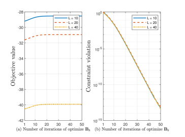
Figure 3: Convergence behavior of Algorithm 2.

Unless specified otherwise, we have chosen the following simulation parameters: a channel bandwidth of $10\mathrm{~{}MHz}$, a noise power density of $-174\mathrm{~{}dBm}/\mathrm{Hz}$, antenna configurations of $N_{\rm{t}}=N_{\rm{r}}=4$ for the BS and $M_{k}=2$ for all CUs. The number of reflecting elements is $L=20$, and the maximum transmit power is $P_{0}=1\mathrm{~{}W}$. We assume that the BS and the RIS are located at $(0\mathrm{~{}m},0\mathrm{~{}m})$, $(15\mathrm{~{}m},0\mathrm{~{}m})$, respectively. The target is located at a spatial angle of $\phi=-20^{\circ}$ w.r.t RIS, at a distance of $5\mathrm{~{}m}$. The radar SNR threshold is set to $\gamma_{0}=30\mathrm{~{}dB}$, CUs are randomly distributed within a circular region centered at $(0\mathrm{~{}m},100\mathrm{~{}m})$ and having a radius of $5\mathrm{~{}m}$.

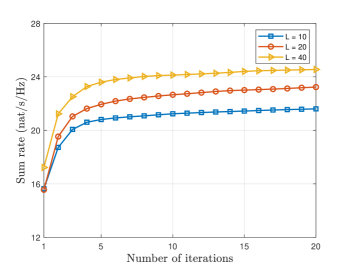
Figure 4: Convergence behavior of Algorithm 3.

We consider the following benchmark schemes to evaluate the RIS-aided DFRC system. We denote ‘Proposed’ as our proposed approach described in Algorithm 3. In the Random RIS scenario (denoted by ‘Random’), the phase shift matrix that satisfies the constraints are randomly generated during initialization. Subsequently, the optimization process focuses exclusively on optimizing the beamforming matrix. Besides, ‘Com-only’ represents that the system only performs the communication function without considering the radar SNR constraint.

IV-A Convergence behavior of the proposed algorithm

First, we evaluate the convergence of the used penalty-based algorithm on optimizing the transmit beamforming matrix $\mathbf{B}_{k}$. Penalty-based algorithm may require careful adjustment of the penalty coefficient $\rho$ and the updated step size $c$ to ensure convergence. The selection of inappropriate parameters may lead to the non-convergence of the optimization problem and the computational workload for solving the problem may substantially rise, resulting in extended computation time, particularly for complex problems. To evaluate the trade-off between convergence performance and computational complexity of Algorithm 2, we plot Fig. 3 with carefully selected $\rho=100$ and $c=0.7$. Fig. 3(a) illustrates the monotonic increase in the objective value (21a) with varying numbers of RIS reflecting elements, specifically $L=10$, $L=20$, and $L=40$, as the number of outer layer iterations grows. With the appropriate parameters $\rho$ and $c$, it is clear that the objective function reaches convergence after approximately $15$ iterations. The penalty terms $\sum_{k=1}^{K}\|{\mathbf{X}_{k}}-\mathbf{B}_{k}\|_{F}^{2}$ and $\sum_{k=1}^{K}\|{\mathbf{Y}_{k}}-\mathbf{V}\mathbf{B}_{k}\|_{F}^{2}$ decrease rapidly with the number of outer layer iterations as shown in Fig. 3(b). As $\rho$ becomes very small, the penalty terms achieve $10^{-13}$ after approximately 50 iterations, indicating the equality constraint (20d) in Problem (20) is eventually satisfied. Thus, Algorithm 2 is guaranteed to converge finally.

In Fig. 4, we investigate the convergence characteristics of Algorithm 3 versus the number of RIS reflecting elements. It is observed from Fig. 4 that the sum rate achieved for various $L$ values increases monotonically with the number of iterations. Additionally, the algorithm converges rapidly and in general 20 iterations are sufficient for the algorithm to achieve a large portion of the converged sum rate.

IV-B Impact of the number of reflective elements on the sum rate

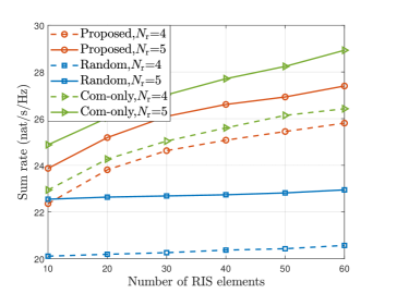
Figure 5: Sum rate versus the number of RIS elements $L$ .

In Fig. 5, we demonstrate the relationship between the achievable sum rate and the number of reflecting elements $L$. As increasing of the number of RIS reflecting elements, a larger sum rate is achieved because of a larger passive beamforming gain. As the number of reflecting elements increases, the performance gap between the the ‘Proposed’ scheme and the ‘Random’ scheme increases. This indicates that it is essential to optimize the phase shift of the RIS especially with a large number of the reflecting elements. Moreover, the DFRC system adds sensing capabilities while having minimal impact on communication than the ‘com-only’ system. At the same time, the gap between the two also reflects the trade-off between communication and radar sensing performance.

Figure 6: Sum rate versus $P_{0}$.

IV-C Impact of the BS transmit power on the sum rate

In this section, we set the number of RIS reflecting elements to $L=20$ and evaluate the relationship between the sum rate and the maximum transmit power of the dual-function BS. In Fig. 6, we observe that the proposed approach achieves a remarkable performance improvement compared to the ‘Random’ scheme. In addition, the scenarios with $N_{\rm{r}}=N_{\rm{t}}=5$ achieve better performance than their counterparts with $N_{\rm{r}}=N_{\rm{t}}=4$ thanks to higher beamforming gain.

IV-D Impact of the BS-CUs path-loss exponent on the sum rate

In the preceding examples, we have configured the path-loss exponents for the BS-CUs links as $\alpha_{\mathrm{BU}}=3.75$. However, in some practical scenarios, especially in an urban environment, surrounding buildings are likely to hinder the BS-CUs path. To this end, Fig. 7 is plotted to evaluate the relationship between the sum rate and the BS-CUs path-loss exponents. The sum rate achieved by all scenarios decreases as $\alpha_{\mathrm{BU}}$ increases, eventually it reaches a plateau with no significant further decrease. This is due to the fact that with the increase of $\alpha_{\mathrm{BU}}$, the signal received at the BS is weaker. However, when $\alpha_{\mathrm{BU}}$ is larger than 5.25, the BS-CUs link cannot operate normally due to severe path loss. At this time, the reflection link provided by RIS can ensure that the sum rate is not less than $8$ $\mathrm{nat/s/Hz}$.

Figure 7: Achievable sum rate versus $\alpha_{\mathrm{BU}}$.

IV-E Impact of the number of quantization bits on the sum rate

In our simulation, we assume that the phase shifts of RIS elements are continuous. However, in practical systems, continuous phase shifts can bring high costs and may even be impossible to achieve. Therefore, discretizing the continuous phase shift of RIS is a more economical method. Specifically, we define $B$ as the number of quantization bits and the corresponding set of discrete phase shifts is

$$\mathcal{A}=\left\{\frac{2\pi m}{2^{B}}\right\},m\in[0,2^{B}-1],m\in\mathbb{N}.$$ (59)

We define $\left\{\phi^{\star}(n)\right\}$ as the optimal continuous phase obtained by the proposed algorithm, and then the discrete phase shifts can be obtained as follows:

$$\hat{\phi}(n)={\mathop{\operatorname{argmin}}\limits_{\left\{\phi\in\mathcal{A}\right\}}}\left\{\left|\phi-\phi^{\star}(n)\right|\right\}.$$ (60)

As shown in Fig. 8, we present the effect of the number of quantization bits on the sum rate. We can see that when $B$ is small, the sum rate increases rapidly with the increase of $B$, while when $B$ is large, the increase of the curve tends to be gradually saturated and close to the sum rate under continuous conditions. The figure shows that six quantization bits can achieve a large portion of that of continuous phase shifts. This shows that the proposed algorithm can effectively reduce hardware cost and power consumption in practical systems.

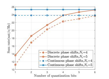
Figure 8: Sum rate versus the number of quantization bits $B$.

IV-F Transmit Beampattern

Fig. 9 presents a comparison of the normalized sensing beampattern for different numbers of reflecting elements of the RIS and diverse radar performance requirements. The beampattern gain from the RIS towards angle $\theta$ is defined as

$$P(\theta)=\left|\mathbf{a}(\theta)^{\rm{H}}{\mathbf{\Theta}}^{\rm{H}}{\bf{G}}{{\bf{x}}}\right|^{2}.$$ (61)

Figure 9: Transmit Beampattern.

Firstly, we compared the beampatterns with $\gamma_{0}=15\mathrm{~{}dB}$ and $\gamma_{0}=25\mathrm{~{}dB}$ when $L=10$, and it can be seen that the latter has lower sidelobe. Meanwhile, if we increase the number of elements in RIS by $L=20$, we can observe that the mainlobe becomes narrower, which further illustrates the benefit of increasing the number of reflecting elements of RIS on sensing performance. Under the same sensing requirements, more power is illuminated in the direction of CUs when the number of the reflecting element is increased to $L=20$.

V CONCLUSION

In this paper, we studied an RIS-aided MU-MIMO DFRC system. We aimed to maximize the achievable sum rate of the CUs by jointly optimizing the BS beamforming matrix and the passive reflecting coefficients of the RIS while satisfying radar SNR constraint, the transmit power constraint of BS and the unit modulus property of the reflecting coefficients of RIS. An AO approach was employed to decouple the optimization variables and split this intractable problem into two subproblems. These subproblems were addressed individually using a penalty-based algorithm and an MM-based algorithm, respectively. Simulation results demonstrated the significant advantages of deploying RIS in ISAC systems. In the future, we will extend our work to active RIS-aided ISAC systems due to the superiority it indicated in[44, 45].

References

• [1] J. Moghaddasi and K. Wu, “Multifunctional transceiver for future radar sensing and radio communicating data-fusion platform,” IEEE Access, vol. 4, pp. 818–838, Feb. 2016.
• [2] D. Ma, N. Shlezinger, T. Huang, Y. Liu, and Y. C. Eldar, “Joint radar-communication strategies for autonomous vehicles: Combining two key automotive technologies,” IEEE Signal Process. Mag., vol. 37, no. 4, pp. 85–97, Jul. 2020.
• [3] L. Zheng, M. Lops, Y. C. Eldar, and X. Wang, “Radar and communication coexistence: An overview: A review of recent methods,” IEEE Signal Process. Mag., vol. 36, no. 5, pp. 85–99, Sep. 2019.
• [4] B. Li, A. P. Petropulu, and W. Trappe, “Optimum co-design for spectrum sharing between matrix completion based MIMO radars and a MIMO communication system,” IEEE Trans. Signal Process., vol. 64, no. 17, pp. 4562–4575, May 2016.
• [5] F. Liu, C. Masouros, A. P. Petropulu, H. Griffiths, and L. Hanzo, “Joint radar and communication design: Applications, state-of-the-art, and the road ahead,” IEEE Trans. Commun., vol. 68, no. 6, pp. 3834–3862, Jun. 2020.
• [6] F. Liu, C. Masouros, A. Li, T. Ratnarajah, and J. Zhou, “MIMO radar and cellular coexistence: A power-efficient approach enabled by interference exploitation,” IEEE Trans. Signal Process., vol. 66, no. 14, pp. 3681–3695, Jul. 2018.
• [7] A. Hassanien, M. G. Amin, Y. D. Zhang, and F. Ahmad, “Dual-function radar-communications: Information embedding using sidelobe control and waveform diversity,” IEEE Trans. Signal Process., vol. 64, no. 8, pp. 2168–2181, Apr. 2015.
• [8] W. Zhou, R. Zhang, G. Chen, and W. Wu, “Integrated sensing and communication waveform design: A survey,” IEEE Open J. Commun. Soc., vol. 3, pp. 1930–1949, Oct. 2022.
• [9] C. Sturm and W. Wiesbeck, “Waveform design and signal processing aspects for fusion of wireless communications and radar sensing,” Proc. IEEE, vol. 99, no. 7, pp. 1236–1259, Jul. 2011.
• [10] S. D. Liyanaarachchi, T. Riihonen, C. B. Barneto, and M. Valkama, “Optimized waveforms for 5G–6G communication with sensing: Theory, simulations and experiments,” IEEE Trans. Wireless Commun., vol. 20, no. 12, pp. 8301–8315, Jun. 2021.
• [11] Y. Zeng, Y. Ma, and S. Sun, “Joint radar-communication with cyclic prefixed single carrier waveforms,” IEEE Trans. Veh. Technol., vol. 69, no. 4, pp. 4069–4079, Apr. 2020.
• [12] K. Wu, J. A. Zhang, X. Huang, and Y. J. Guo, “OTFS-based joint communication and sensing for future industrial IoT,” IEEE Internet Things J., Feb. 2021.
• [13] R. Xie, K. Luo, and T. Jiang, “Waveform design for LFM-MPSK-based integrated radar and communication toward IoT applications,” IEEE Internet Things J., vol. 9, no. 7, pp. 5128–5141, Aug. 2021.
• [14] M. Nowak, M. Wicks, Z. Zhang, and Z. Wu, “Co-designed radar-communication using linear frequency modulation waveform,” IEEE Aerosp. Electron. Syst. Mag., vol. 31, no. 10, pp. 28–35, Oct. 2016.
• [15] Q. Wang and S. Xu, “Vehicle width detection based on millimeter-wave LFMCW radar for autonomous driving,” in 2022 IEEE 95th Vehicular Technology Conference:(VTC2022-Spring).   IEEE, Aug. 2022, pp. 1–6.
• [16] X. Liu, T. Huang, N. Shlezinger, Y. Liu, J. Zhou, and Y. C. Eldar, “Joint transmit beamforming for multiuser MIMO communications and MIMO radar,” IEEE Trans. Signal Process., vol. 68, pp. 3929–3944, Jun. 2020.
• [17] J. Yang, G. Cui, X. Yu, and L. Kong, “Dual-use signal design for radar and communication via ambiguity function sidelobe control,” IEEE Trans. Veh. Technol., vol. 69, no. 9, pp. 9781–9794, Sep. 2020.
• [18] F. Dong, W. Wang, X. Li, F. Liu, S. Chen, and L. Hanzo, “Joint beamforming design for dual-functional MIMO radar and communication systems guaranteeing physical layer security,” IEEE Trans. Green Commun. Netw., vol. 7, no. 1, pp. 537–549, Jan. 2023.
• [19] Q. Wu and R. Zhang, “Towards smart and reconfigurable environment: Intelligent reflecting surface aided wireless network,” IEEE Commun. Mag., vol. 58, no. 1, pp. 106–112, Jan. 2019.
• [20] T. J. Cui, M. Q. Qi, X. Wan, J. Zhao, and Q. Cheng, “Coding metamaterials, digital metamaterials and programmable metamaterials,” Light Sci. Appl., vol. 3, no. 10, pp. e218–e218, Oct. 2014.
• [21] N. Yu, P. Genevet, M. A. Kats, F. Aieta, J.-P. Tetienne, F. Capasso, and Z. Gaburro, “Light propagation with phase discontinuities: generalized laws of reflection and refraction,” Science, vol. 334, no. 6054, pp. 333–337, Sep. 2011.
• [22] C. Pan, G. Zhou, K. Zhi, S. Hong, T. Wu, Y. Pan, H. Ren, M. D. Renzo, A. Lee Swindlehurst, R. Zhang, and A. Y. Zhang, “An overview of signal processing techniques for RIS/IRS-aided wireless systems,” IEEE J.Sel.Top. Signal Process., vol. 16, no. 5, pp. 883–917, Aug. 2022.
• [23] C. Pan, H. Ren, K. Wang, W. Xu, M. Elkashlan, A. Nallanathan, and L. Hanzo, “Multicell MIMO communications relying on intelligent reflecting surfaces,” IEEE Trans. Wireless Commun., vol. 19, no. 8, pp. 5218–5233, May 2020.
• [24] Z. Zhu, Z. Li, Z. Chu, G. Sun, W. Hao, P. Xiao, and I. Lee, “Resource allocation for IRS assisted mmwave integrated sensing and communication systems,” in ICC 2022 - IEEE International Conference on Communications, May 2022, pp. 2333–2338.
• [25] X. Wang, Z. Fei, Z. Zheng, and J. Guo, “Joint waveform design and passive beamforming for RIS-assisted dual-functional radar-communication system,” IEEE Trans. Veh. Technol., vol. 70, no. 5, pp. 5131–5136, Apr. 2021.
• [26] Z.-M. Jiang, M. Rihan, P. Zhang, L. Huang, Q. Deng, J. Zhang, and E. M. Mohamed, “Intelligent reflecting surface aided dual-function radar and communication system,” IEEE Syst. J., vol. 16, no. 1, pp. 475–486, Mar. 2021.
• [27] X. Song, D. Zhao, H. Hua, T. X. Han, X. Yang, and J. Xu, “Joint transmit and reflective beamforming for IRS-assisted integrated sensing and communication,” in 2022 IEEE Wireless Communications and Networking Conference (WCNC).   IEEE, Apr. 2022, pp. 189–194.
• [28] Y. Li and A. Petropulu, “Dual-function radar-communication system aided by intelligent reflecting surfaces,” in 2022 IEEE 12th Sensor Array and Multichannel Signal Processing Workshop (SAM).   IEEE, Jun. 2022, pp. 126–130.
• [29] H. Zhang, “Joint waveform and phase shift design for RIS-assisted integrated sensing and communication based on mutual information,” IEEE Commun. Lett., vol. 26, no. 10, pp. 2317–2321, Oct. 2022.
• [30] H. Luo, R. Liu, M. Li, and Q. Liu, “RIS-aided integrated sensing and communication: Joint beamforming and reflection design,” IEEE Trans. Veh. Technol., Feb. 2023.
• [31] L. Chen, Z. Wang, Y. Du, Y. Chen, and F. R. Yu, “Generalized transceiver beamforming for DFRC with MIMO radar and MU-MIMO communication,” IEEE J. Sel. Areas Commun., vol. 40, no. 6, pp. 1795–1808, Mar. 2022.
• [32] G. Zhou, C. Pan, H. Ren, P. Popovski, and A. L. Swindlehurst, “Channel estimation for RIS-aided multiuser millimeter-wave systems,” IEEE Trans. Signal Process., vol. 70, pp. 1478–1492, Mar. 2022.
• [33] J. Capon, “High-resolution frequency-wavenumber spectrum analysis,” Proc. IEEE, vol. 57, no. 8, pp. 1408–1418, Aug. 1969.
• [34] Q. Shi, M. Razaviyayn, Z.-Q. Luo, and C. He, “An iteratively weighted mmse approach to distributed sum-utility maximization for a MIMO interfering broadcast channel,” IEEE Trans. Signal Process., vol. 59, no. 9, pp. 4331–4340, Apr. 2011.
• [35] C. Pan, H. Ren, K. Wang, M. Elkashlan, A. Nallanathan, J. Wang, and L. Hanzo, “Intelligent reflecting surface aided MIMO broadcasting for simultaneous wireless information and power transfer,” IEEE J.Sel. Areas Commun., vol. 38, no. 8, pp. 1719–1734, Jun. 2020.
• [36] Z. Peng, Z. Zhang, C. Pan, L. Li, and A. L. Swindlehurst, “Multiuser full-duplex two-way communications via intelligent reflecting surface,” IEEE Trans. Signal Process., vol. 69, pp. 837–851, Jan. 2021.
• [37] M. Hua, Q. Wu, C. He, S. Ma, and W. Chen, “Joint active and passive beamforming design for IRS-aided radar-communication,” IEEE Trans. Wireless Commun., vol. 22, no. 4, pp. 2278–2294, Apr. 2022.
• [38] S. Boyd, S. P. Boyd, and L. Vandenberghe, Convex optimization.   Cambridge university press, 2004.
• [39] X.-D. Zhang, Matrix analysis and applications.   Cambridge University Press, 2017.
• [40] Y. Sun, P. Babu, and D. P. Palomar, “Majorization-minimization algorithms in signal processing, communications, and machine learning,” IEEE Trans. Signal Process., vol. 65, no. 3, pp. 794–816, Feb. 2016.
• [41] I. M. Bomze, V. F. Demyanov, R. Fletcher, T. Terlaky, I. Pólik, and T. Terlaky, “Interior point methods for nonlinear optimization,” Nonlinear Optimization. Berlin, Germany: Springer, pp. 215–276, Jan. 2010.
• [42] A. Ben-Tal and A. Nemirovski, Lectures on modern convex optimization: analysis, algorithms, and engineering applications.   SIAM, 2001.
• [43] G. Zhou, C. Pan, H. Ren, K. Wang, and A. Nallanathan, “A framework of robust transmission design for IRS-aided MISO communications with imperfect cascaded channels,” IEEE Trans. Signal Process., vol. 68, pp. 5092–5106, Aug. 2020.
• [44] Z. Yu, H. Ren, C. Pan, G. Zhou, B. Wang, M. Dong, and J. Wang, “Active RIS aided ISAC systems: Beamforming design and performance analysis,” IEEE Trans. Commun., pp. 1–1, Nov. 2023.
• [45] K. Zhi, C. Pan, H. Ren, K. K. Chai, and M. Elkashlan, “Active ris versus passive ris: Which is superior with the same power budget?” IEEE Commun. Lett., vol. 26, no. 5, pp. 1150–1154, Mar. 2022.