How Much is Unseen Depends Chiefly on Information About the Seen

Abstract

It might seem counter-intuitive at first: We find that, in expectation, the proportion of data points in an unknown population—that belong to classes that do not appear in the training data—is almost entirely determined by the number $f_{k}$ of classes that do appear in the training data the same number of times. While in theory we show that the difference of the induced estimator decays exponentially in the size of the sample, in practice the high variance prevents us from using it directly for an estimator of the sample coverage. However, our precise characterization of the dependency between $f_{k}$’s induces a large search space of different representations of the expected value, which can be deterministically instantiated as estimators. Hence, we turn to optimization and develop a genetic algorithm that, given only the sample, searches for an estimator with minimal mean-squared error (MSE). In our experiments, our genetic algorithm discovers estimators that have a substantially smaller MSE than the state-of-the-art Good-Turing estimator. This holds for over 96% of runs when there are at least as many samples as classes. Our estimators’ MSE is roughly 80% of the Good-Turing estimator’s.

1 Introduction

Suppose, we are drawing balls with replacement from an urn with colored balls. What is the proportion of balls in that urn that have a color not observed in the sample; or equivalently, what is the probability that the next ball has a previously unobserved color? What is the distribution of rarely observed colors in that urn? These questions represent a fundamental problem in machine learning: How can we extrapolate from properties of the training data to properties of the unseen, underlying distribution of the data?

1.1 Background

Consider a multinomial distribution $p=\langle p_{1},\cdots p_{S}\rangle$ over a support set $\mathcal{X}$ where support size $S=|\mathcal{X}|$ and probability values are unknown. Let $X^{n}=\langle X_{1},\cdots X_{n}\rangle$ be a set of independent and identically distributed random variables representing the sequence of elements observed in $n$ samples from $p$. Let $N_{x}$ be the number of times element $x\in\mathcal{X}$ is observed in the sample $X^{n}$. For $k:0\leq k\leq n$, let $\Phi_{k}$ be the number of elements appearing exactly $k$ times in $X^{n}$.

$$N_{x}=\sum_{i=1}^{n}\mathbbm{1}(X_{i}=x)\text{\quad and \quad}\Phi_{k}=\sum_{x\in\mathcal{X}}\mathbbm{1}(N_{x}=k)$$

Let $f_{k}(n)$ be the expected value of $\Phi_{k}$ (Good, 1953), i.e.,

$$f_{k}(n)={n\choose k}\sum_{x\in\mathcal{X}}p_{x}^{k}(1-p_{x})^{n-k}=\mathbb{E}\left[\Phi_{k}\right]$$

Estimating the multinomial. Suppose, we want to estimate $p$. We cannot expect all elements to exist in $X^{n}$. While the empirical estimator $\hat{p}_{x}^{\text{Emp}}=N_{x}/n$ is generally unbiased, $\hat{p}_{x}^{\text{Emp}}$ distributes the entire probability mass only over the observed elements. This leaves a “missing probability mass” over the unobserved elements. In particular, $\hat{p}_{x}^{\text{Emp}}$ given that $N_{x}>0$ overestimates $p_{x}$, i.e., for observed elements

$$\mathbb{E}\left[\left.\frac{N_{x}}{n}\ \right|\ N_{x}>0\right] =\frac{p_{x}}{1-(1-p_{x})^{n}}.$$

We notice that the bias increases as $p_{x}$ decreases. Bias is maximized for the rarest observed element.

Missing mass, realizability, and natural estimation. Good and Turing (GT) (Good, 1953) discovered that the expected value of the probability $M_{k}=\sum_{x\in\mathcal{X}}p_{x}\mathbbm{1}(N_{x}=k)$ that the $(n+1)$-th observation $X_{n+1}$ is an element that has been observed exactly $k$ times in $X^{n}$ (incl. $k=0$) is a function of the expected number of colors $f_{k+1}(n+1)$ that will be observed $k+1$ times in an enlarged sample $X^{n}\cup X_{n+1}$.

$$\mathbb{E}\left[M_{k}\right]=\frac{k+1}{n+1}f_{k+1}(n+1).$$ (1)

We also call $M_{k}$ as total probability mass over the elements that have been observed exactly $k$ times. Since our sample $X^{n}$ is only of size $n$, GT suggested to estimate $f_{k+1}(n+1)$ using $\Phi_{k+1}$. Concretely, $\hat{M}_{k}^{G}=\frac{k+1}{n}\Phi_{k+1}$.

For $k=0$, $M_{0}$ gives the “missing” (probability) mass over the elements not in the sample. In genetics and biostatistics, the complement $1-M_{0}$ measures sample coverage, i.e., the proportion of individuals in the population belonging to a species not observed in the sample (Chao & Jost, 2012). In the context of supervised machine learning, assuming the training data is a random sample, the sample coverage of the training data gives the proportion of all data (seen or unseen) with labels not observed in the training data.

Using an estimate $\hat{M}_{k}$ of $M_{k}$, we estimate the probability $p_{x}$ of an element $x\in\mathcal{X}$ that appears $k$ times as $\hat{M}_{k}/\Phi_{k}$. The estimation of $p$ in the presence of unseen elements $x\not\in X^{n}$ is a fundamental problem in machine learning (Orlitsky et al., 2003; Orlitsky & Suresh, 2015; Painsky, 2022; Acharya et al., 2013; Hao & Li, 2020). For instance, in natural language processing the estimation of the probability of a given sequence of words occurring in a sentence is the main challenge of language models, particularly in the presence of sequences that appear in the training data rarely or not at all. Different smoothing and backoff techniques have been developed to tackle this data sparsity challenge.

A natural estimator of $p_{x}$ assigns the same probability to all elements $x$ appearing the same number of times in the sample $X^{n}$ (Orlitsky & Suresh, 2015). For $k>0$, $\hat{p}_{x}=M_{k}/\Phi_{k}$ gives the hypothetical best natural estimator of $p_{x}$ for every element $x$ that has been observed $k$ times.

Bias of Good-Turing (GT). In terms of bias, Juan and Lo (Juang & Lo, 1994) observe that the GT estimator $\hat{M}_{k}^{G}=\frac{k+1}{n}\Phi_{k+1}$ is an unbiased estimate of $M_{k}(X^{n-1})$, i.e., where the $n$-th sample was deleted from $X^{n}$ and find:

$$\left|\mathbb{E}\left[\hat{M}_{k}^{G}-M_{k}\right]\right| =\left|\mathbb{E}\left[M_{k}(X^{n-1})-M_{k}(X^{n})\right]\right|$$

$$\leq\frac{k+2}{n+1}=\mathcal{O}\left(\frac{1}{n}\right).$$

Convergence of GT. McAllester and Schapire (McAllester & Schapire, 2000) analyzed the convergence. With high probability,

$$|\hat{M}_{k}^{G}-M_{k}(n)|$$

$$=_{\delta}\begin{cases}\mathcal{O}\left(1/\sqrt{n}\right)&\text{for $k=0$ (missing mass)}\\ \mathcal{O}\left(\log(n)/\sqrt{n}\right)&\text{for small $k$ (rare elements)}\\ \mathcal{O}\left(k/\sqrt{n}\right)&\text{for large $k$ (abundant elements).}\end{cases}$$

This result was improved by Drukh and Mansour (Drukh & Mansour, 2004) and more recently by Painsky (Painsky, 2022) who showed that GT estimator converges at a rate of $\mathcal{O}(1/\sqrt{n})$ for all $k$ based on worst-case mean squared error analysis.

Competitiveness of GT. Using the Poisson approximation, Orlitsky and Suresh (Orlitsky & Suresh, 2015) showed that natural estimators from GT, i.e., $\hat{p}_{x}^{G}=\hat{M}_{N_{x}}^{G}/\Phi_{N_{x}}$, performs close to the best natural estimator. Regret, the metric of the competitiveness of an estimator against the best natural estimator, is measured as KL divergence between the estimate $\hat{p}$ and the actual distribution $p$, $D_{KL}(\hat{p}||p)$. Orlitsky and Suresh also showed that finding the best natural estimator for $p$ is same as finding the best estimator for $M=\{M_{k}\}_{k=0}^{n}$.

Poisson approximation. The Poisson approximation with parameter $\lambda_{x}=p_{x}n$ has often been used to tackle a major challenge in the formal analysis of the missing mass and natural estimators (Orlitsky & Suresh, 2015; Orlitsky et al., 2016; Acharya et al., 2013; Efron & Thisted, 1976; Valiant & Valiant, 2016; Good, 1953; Good & Toulmin, 1956; Hao & Li, 2020). The challenge is the dependencies between frequencies $N_{x}$ for different elements $x\in\mathcal{X}$. In this Poisson Product model, a continuous-time sampling scheme with $S=|\mathcal{X}|$ independent Poisson distributions is considered where the frequency $N_{x}$ of an element $x$ is represented as a Poisson random variable with mean $p_{x}n$. In other words, in the Poisson approximation, the frequencies $N_{x}$ are modelled as independent random variables. Consequently, GT estimator is an unbiased estimator for the Poisson Product model (Orlitsky et al., 2016), yet it is biased in the multinomial distribution (Juang & Lo, 1994). Hence, we tackle the dependencies between frequencies analytically, without approximation via the Poisson Product model.

1.2 Contribution of the Paper

In this paper, we reinforce the foundations of multinomial distribution estimation with a precise characterization of the the dependencies between $N_{x}=\sum_{i=1}^{n}\mathbbm{1}(X_{i}=x)$ across different $x\in\mathcal{X}$ (rather than assuming independence and using the Poisson approximation). The theoretical analysis is based on the expected value of the frequency of frequencies $\mathbb{E}\left[\Phi_{k}\right]=f_{k}(n)$ between different $k$ and $n$, which is

$$\frac{f_{k}(n)}{{n\choose k}}=\frac{f_{k}(n+1)}{{n+1\choose k}}-\frac{f_{k+1}(n+1)}{{n+1\choose k+1}}.$$ (2)

Exploring this new theoretical tool, we bring two contributions to the estimation of the total probability mass $M_{k}$ for any $k:0\leq k\leq n$. Firstly, we show exactly to what extent $\mathbb{E}\left[M_{k}\right]$ can be estimated from the sample $X^{n}$ and how much remains to be estimated from the underlying distribution $p$ and the number of elements $|\mathcal{X}|$. Specifically, we show the following.

Theorem 1.1.

$$\mathbb{E}\left[M_{k}\right]={n\choose k}\left[\sum_{i=1}^{n-k}(-1)^{i-1}f_{k+i}(n)\left/{n\choose k+i}\right.\right]+R_{n,k}$$

where $R_{n,k}={n\choose k}(-1)^{n-k}f_{n+1}(n+1)$ is the remainder.

This decomposition shows that the GT estimator is the first term of $\mathbb{E}\left[M_{k}\right]$ using the plug-in estimator $\Phi_{1}$ for $f_{1}(n)$. Hence, it gives the exact bias of the GT estimator in the multinomial setting (which would incorrectly be identified as unbiased using the Poisson approximation).

Our second contribution is the development of a class of natural estimators. We start by defining a nearly unbiased estimator $\hat{M}_{k}^{B}={n\choose k}\left[\sum_{i=1}^{n-k}(-1)^{i-1}\Phi_{k+i}\left/{n\choose k+i}\right.\right]$ that uses the plug-in estimator $\Phi_{l}$ for $f_{l}(n)$ in Theorem 1.1 and drops $R_{n,k}$. While the bias of $\hat{M}_{k}^{B}$ decays exponentially, the variance of $\hat{M}_{k}^{B}$ is too high to be practical.

We observe that we can cast the estimation of the expected total mass as an optimization problem. From Theorem 1.1 and Eqn. 2, we can see that there are many representations of $\mathbb{E}\left[M_{k}\right]$, all of which suggest different estimators for $\mathbb{E}\left[M_{k}\right]$. We introduce a deterministic method to construct a unique estimator from a representation, and show how to estimate the mean squared error (MSE) for such an estimator. Equipped with a large search space of representations and a fitness function to estimate the MSE of a candidate estimator, we develop a genetic algorithm that finds an estimator with a minimal MSE (and at most N terms).

We compare the performance of the minimal-bias estimator $\hat{M}_{k}^{B}$ and the minimal-MSE estimators discovered by our genetic algorith to the that of the widely used GT estimator on a variety of multinomial distributions used for evaluation in previous work. Our results show that 1) the minimal-bias estimator has a substantially smaller bias than the GT estimator by thousands of order of magnitude, 2) Our genetic algorithm can produce estimators with MSE smaller than the GT estimator over 96% of the time when there are at least as many samples as classes; their MSE is roughly 80% of the GT estimator. We also publish all data and scripts to reproduce our results.

2 Dependencies Between Frequencies $N_{x}$

Firstly, we propose a new, distribution-free methodology for reasoning about properties of estimators of the missing and total probability masses for multinomial distributions. The main challenge for the statistical analysis of $M_{k}$ has been reasoning in the presence of dependencies between frequencies $N_{x}$ for different elements $x\in\mathcal{X}$. As discussed in Section 1.1, a Poisson approximation with parameter $\lambda_{x}=p_{x}n$ is often used to render these frequencies as independent (Orlitsky & Suresh, 2015; Orlitsky et al., 2016; Acharya et al., 2013; Efron & Thisted, 1976; Valiant & Valiant, 2016; Good, 1953; Good & Toulmin, 1956; Hao & Li, 2020). In the following, we tackle this challenge by formalizing these dependencies between frequencies. Thus, we establish a link between the expected values of the corresponding total probability masses.

2.1 Dependency Among Frequencies

Recall that the expected value $f_{k}(n)$ of the number of elements $\Phi_{k}$ that appear exactly $k$ times in the sample $X^{n}$ is defined as $f_{k}(n)=\sum_{x\in\mathcal{X}}\binom{n}{k}p_{x}^{k}(1-p_{x})^{n-k}$. For convencience, let $g_{k}(n)=f_{k}(n)/{n\choose k}$. We notice the following relationship among $k$ and $n$:

$$g_{k}(n+1) =\sum_{x=1}^{S}p_{x}^{k}(1-p_{x})^{n-k}\cdot(1-p_{x})$$

$$=g_{k}(n)-g_{k+1}(n+1)$$ (3)

$$=\sum_{i=0}^{n-k}(-1)^{i}g_{k+i}(n)+(-1)^{n-k+1}g_{n+1}(n+1)$$

We can now write the expected value $\mathbb{E}\left[M_{k}\right]$ of the total probability mass in terms of the frequencies with which different elements $x\in\mathcal{X}$ have been observed in the sample $X^{n}$ of size $n$ as follows

$$\mathbb{E}\left[M_{k}\right] =\sum_{x\in\mathcal{X}}\binom{n}{k}p_{x}^{k+1}(1-p_{x})^{n-k}$$

$$={n\choose k}g_{k+1}(n+1)$$ (4)

$$={n\choose k}\left[\sum_{i=1}^{n-k}(-1)^{i-1}g_{k+i}(n)\right]+R_{n,k}$$ (5)

where $R_{n,k}={n\choose k}(-1)^{n-k}f_{n+1}(n+1)$ is a remainder term. This demonstrates Theorem 1.1.

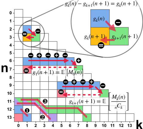
Figure 1: Lower triangle matrix of $g_{k}(n)$.

Figure 1 illustrates the relationship between the expected frequency of frequencies $f_{k}(n)=g_{k}(n)/{n\choose k}$, the frequency $k$, and the sample size $n$. The y- and x-axis represents the sample size $n$ and the frequency $k$, respectively. As per Eqn. (3), for every 2x2 lower triangle matrix, the value of the lower left cell ($g_{k}(n+1)$) is value of the upper left cell ($g_{k}(n)$) minus the value of the lower right cell ($g_{k+1}(n+1)$).

We can use this visualization to quickly see how to rewrite $g_{k}(n)$ as an alternating sum of values of the cells in the upper row, starting from the cell in the same column to the rightmost cell, and adding/subtracting the value of the rightmost cell in the current row. For instance, the value $g_{0}(13)$ in the bottom red cell (row $n=13$, column $k=0$) in the figure can be equally calculated as the various linear combinations of its surrounding cells: (1) with $g_{0}(12)$ and $g_{1}(13)$ (blue colored), (2) with $g_{0}(11)$, $g_{1}(11)$, $\cdots$, $g_{4}(13)$ (purple colored), or (3) with $g_{0}(11)$, $g_{1}(11)$, $\cdots$, $g_{8}(13)$ (green colored).

Missing Mass. The missing probability mass $M_{0}$ gives the proportion of all possible observations for which the elements $x\in\mathcal{X}$ have not been observed in $X^{n}$. By Eqn. (4) and (5), the expected value of $M_{0}$ is

$$\mathbb{E}\left[M_{0}\right] =g_{1}(n+1)$$

$$=\left[\sum_{k=1}^{n}(-1)^{k-1}g_{k}(n)\right]+(-1)^{n}f_{n+1}(n+1).$$

The values in the second column of Figure 1 ($k=1$) represents the expected values of missing mass; $\mathbb{E}\left[M_{0}\right]$ being the cumulative sum of $(-1)^{k-1}g_{k}(n)$ is intuitively clear from the figure (the red cell in the row $n=7$). It is here where we observe that $\mathbb{E}\left[M_{0}\right]=g_{1}(n+1)$ is almost entirely determined by the $g_{*}(n)$, the expected frequencies of frequencies in the sample $X^{n}$, and not by the number of elements $|\mathcal{X}|$ or their underlying distribution $p$. In fact, the influence of $p$ in the remainder term decays exponentially, i.e., $f_{n+1}(n+1)=\sum_{x\in\mathcal{X}}p_{x}^{n+1}\leq\sum_{x\in\mathcal{X}}\left(e^{1-p_{x}}\right)^{-n-1}$ which is dominated by the discovery probability of the most abundant element $\max(p)$.

Total Mass. Similarly, the expected value of the total probability mass $\mathbb{E}\left[M_{k}\right]$ (the red cell in the row $n=10$), which is equal to ${n\choose k}g_{k+1}(n+1)$, is almost entirely determined by the expected frequencies of the sample $X^{n}$ with remainder $R_{n,k}={n\choose k}\sum_{x\in\mathcal{X}}p_{x}^{n+1}$.

3 A Large Class of Estimators

From the representation of $\mathbb{E}\left[M_{k}\right]$ in terms of frequencies in Eqn. (4) and the relationship across frequencies in Eqn. (3), we can see that there is a large number of representations of the expected total probability mass $\mathbb{E}\left[M_{k}\right]$. Each representation might suggest different estimators.

We start by defining the minimal bias estimator $\hat{M}_{k}^{B}$ from the representation in Eqn. (5) and explore its properties.

3.1 Estimator with Exponentially Decaying Bias

Let

$$\hat{M}_{k}^{B}=-{n\choose k}\sum_{i=1}^{n-k}\frac{(-1)^{i}\Phi_{k+i}}{{n\choose k+i}}$$

Bias. For some constant $k:0\leq k\leq n$ and some constant $\mathbf{c}>1$, the bias of $\hat{M}_{k}^{B}$ is in the order of $\mathcal{O}(n^{k}\mathbf{c}^{-n})$, i.e.,

$$\mathbb{E}\left[\hat{M}_{k}^{B}-M_{k}\right] =-R_{n,k}=(-1)^{n-k-1}{n\choose k}\sum_{x\in\mathcal{X}}p_{x}^{n+1}$$

$$\left|\mathbb{E}\left[\hat{M}_{k}^{B}-M_{k}\right]\right| \leq{n\choose k}\sum_{x\in\mathcal{X}}\mathbf{c}_{x}^{-n}\leq n^{k}\sum_{x\in\mathcal{X}}\mathbf{c}_{x}^{-n}$$

where $\mathbf{c}_{x}>1$ for all $x\in\mathcal{X}$ are constants.

Variance. The variance of $\hat{M}_{k}^{B}$ is given by the variances and covariances of the frequencies $\Phi_{k+i}$ for $i=1,\cdots,n-k$. Under the certain conditions, the variance of $\hat{M}_{k}^{B}$ also decays exponentially in $n$.

Theorem 3.1.

The variance of $\hat{M}_{k}^{B}$ decreases exponentially with $n$ if $p_{\max}<0.5$ or $\frac{(1-p_{\max})(1-p_{\min})}{p_{\max}}<1$, where $p_{\max}=\max_{x\in\mathcal{X}}p_{x}$ and $p_{\min}=\min_{x\in\mathcal{X}}p_{x}$.

The proof is postponed to Appendix B.

Comparison to Good-Turing (GT). The bias of $\hat{M}_{k}^{B}$ not only decays exponentially in $n$ but is also smaller than that of GT estimator $\hat{M}_{k}^{G}$ by an exponential factor. For a simpler variant of GT estimator, $\hat{M}_{k}^{G^{\prime}}=\frac{k+1}{n-k}\Phi_{k+1}$ (suggested in (McAllester & Schapire, 2000)), which corresponds to the first term in the expected total probability mass $\mathbb{E}\left[M_{k}\right]$ in Eqn. (5), we show that its bias is larger by an exponential factor than the absolute bias of $\hat{M}_{k}^{B}$. To see this, we provide bounds on the individual sums and then on the bias ratio:

$$\text{\emph{Bias}}_{G^{\prime}}=\mathbb{E}\left[\hat{M}_{k}^{G^{\prime}}-M_{k}\right] \geq{n\choose k}p_{\min}^{k+2}(1-p_{\min})^{n-k-1}$$ (6)

$$|\text{\emph{Bias}}_{B}|=\left|\mathbb{E}\left[\hat{M}_{k}^{B}-M_{k}\right]\right| \leq{n\choose k}Sp_{\max}^{n+1}$$ (7)

where $S=|\mathcal{X}|$, such that

$$\left|\frac{\text{\emph{Bias}}_{G^{\prime}}}{\text{\emph{Bias}}_{B}}\right| \geq\frac{p^{k+2}_{\min}}{Sp^{k+2}_{\max}}\left(\frac{1-p_{\min}}{p_{\max}}\right)^{n-k-1}.$$

Notice that $(1-p_{\min})/p_{\max}>1$ for all distributions over $\mathcal{X}$, except where $S=2$ and $p=\{0.5,0.5\}$. The same can be shown for the original GT estimator $\hat{M}_{k}^{G}=\frac{k+1}{n}\Phi_{k+1}$ for a sufficiently large sample size (see Appendix A).

Example (Missing mass for the uniform). Suppose, we seek to estimate the missing mass from a sequence of elements $X^{n}$ observed in $n$ samples from the uniform distribution; $p_{x}=1/S$ for all $x\in\mathcal{X}$. $\hat{M}_{0}^{G}$ overestimates $M_{0}$ on the average by $(S-1)^{n-1}/S^{n}$ while our new estimator $\hat{M}_{0}^{B}$ has a bias of $(-1)^{n}/S^{n}$. Hence, for the uniform distribution, our estimator exhibits a bias that is lower by a factor of $1/(S-1)^{n-1}$.

While the bias of our estimator $\hat{M}_{k}^{B}$ is lower than that of $\hat{M}_{0}^{G}$ by an exponential factor, the variance is higher. The variance of $\hat{M}_{k}^{B}$ depends on the variances of and covariances between $\Phi_{k+1},\Phi_{k+2},\ldots,\Phi_{n}$, i.e.,

$$\begin{split}\mathrm{Var}\left(\hat{M}_{k}^{B}\right)&=\sum_{i=1}^{n-k}c_{i}^{2}\mathrm{Var}\left(\Phi_{k+i}\right)\\ &+\sum_{i\neq j}(-1)^{i+j}c_{i}c_{j}\mathrm{Cov}\left(\Phi_{k+i},\Phi_{k+j}\right),\end{split}$$ (8)

where $c_{i}=\left.\binom{n}{k}\right/\binom{n}{k+i}$. In contrast, the variance of $\hat{M}_{k}^{G}$ depends only on the variance of $\Phi_{k+1}$. In the empirical study, we investigate the difference of the two estimators in terms of the bias and the variance.

3.2 Estimation with Minimal MSE as Search Problem

There are many representations of $\mathbb{E}\left[M_{k}\right]={n\choose k}g_{k+1}(n+1)$ that can be constructed by recursively rewriting terms according to the dependency among frequencies we identified (cf. Eqn. (3 & 4)). The representation used to construct our minimal-bias estimator $\hat{M}_{k}^{B}$ was one of them. However, we notice that the variance of $\hat{M}_{k}^{B}$ is too high to be practical. To find a representation from which an estimator with a minimal mean squared error (MSE) can be derived, we cast the efficient estimation of $M_{k}$ as an optimization problem. To efficiently navigate the large search space of representations of $\mathbb{E}\left[M_{k}\right]$, we develop a genetic algorithm.

Search space. Let $\mathbb{E}\left[M_{k}\right]$ be represented by a suitable choice of coefficients $\alpha_{i,j}$ such that

$$\mathbb{E}\left[M_{k}\right]=\sum_{i=1}^{n+1}\sum_{j=i}^{n+1}\alpha_{i,j}g_{i}(j).$$ (9)

One representation of $\mathbb{E}\left[M_{k}\right]={n\choose k}g_{k+1}(n+1)$ is

$$r_{0}=\left\{\alpha_{i,j}=\begin{cases}\binom{n}{k}&\text{for $i=k+1$ and $j={n+1}$}\\ 0&\text{otherwise.}\hfill\end{cases}\right\}$$ (10)

Mutation. Given any representation $r$ of $\mathbb{E}\left[M_{k}\right]$, we can construct a new representation $r^{\prime}$ of $\mathbb{E}\left[M_{k}\right]$, s.t. Eqn. (9) holds by recursively considering the following identities:

$$\alpha_{i,j}\cdot g_{i}(j) =\alpha_{i,j}\cdot((1-\delta)g_{i}(j)+\delta g_{i}(j))$$ (11)

$$=\alpha_{i,j}\cdot(g_{i}(j+1)+g_{i+1}(j+1))$$ (12)

$$=\alpha_{i,j}\cdot(g_{i}(j-1)-g_{i+1}(j))$$ (13)

$$=\alpha_{i,j}\cdot(g_{i-1}(j-1)+g_{i-1}(j))$$ (14)

for any choice of $\delta:0\leq\delta\leq 1$. Importantly, after applying these identities, we must work out the new coefficients accordingly. For instance, applying Eqn. (11) with $\delta=0.5$ and Eqn. (13) to $r_{0}$, we obtain the following representation $r_{1}$ of $\mathbb{E}\left[M_{k}\right]$:

$$r_{1}=\left\{\alpha_{i,j}=\begin{cases}\left.\binom{n}{k}\right/2&\text{for $i=k+1$ and $j={n+1}$}\\ \left.\binom{n}{k}\right/2&\text{for $i=k+1$ and $j={n}$}\\ \left.-\binom{n}{k}\right/2&\text{for $i=k+2$ and $j={n+1}$}\\ 0&\text{otherwise.}\hfill\end{cases}\right\}$$

Algorithm 1 Genetic Algorithm

0:  Target frequency $k$, Sample $X^{n}$

0:  Iteration limit $G$, mutant size $m$

1:  Population $P_{0}=\{r_{0}\}$

2:  Fitness $f^{\text{best}}=f_{0}=\text{\emph{fitness}}(r_{0})$

3:  Limit $G_{L}=G$

4:  for $g$ from $1$ to $G_{L}$ do

5:     $P=\text{\emph{selectTopM}}(P_{g-1},m)$

6:     $P^{\prime}=\text{\emph{lapply}}(P,\text{\emph{mutate}})$

7:     $P_{g}=P^{\prime}\cup\{r_{0}\}\cup\text{\emph{selectTopM}}(P_{g-1},3)$

8:     $f_{g}=\min(\text{\emph{lapply}}(P_{g},\text{\emph{fitness}}))$

9:     if $(g=G_{L})\wedge((f_{g}=f_{0})\vee(f^{\text{best}}>0.95\cdot f_{g}))$ then

10:        $G_{L}=G_{L}+G$

11:        $f^{\text{best}}=f_{g}$

12:     end if

13:  end for

14:  Estimator $\hat{M}_{k}^{\text{Evo}}=\text{\emph{instantiate}}(\text{\emph{selectTopM}}(P_{G_{L}},1))$

14:  Minimal-MSE Estimator $\hat{M}_{k}^{\text{Evo}}$

Estimator instantiation. To construct a unique estimator $\hat{M}_{k}^{r}$ of $M_{k}$ from a representation $r$ of $\mathbb{E}\left[M_{k}\right]$, we propose a deterministic method. But first, we define our random variables on subsamples of $X^{n}$. For any $m\leq n$, let $N_{x}(m)$ be the number of times element $x\in\mathcal{X}$ is observed in the subsample $X^{m}=\langle X_{1},\cdots X_{m}\rangle$ of $X^{n}$. Let $\Phi_{k}(m)$ be the number of elements appearing exactly $k$ times in $X^{m}$, i.e.,

$$N_{x}(m) =\sum_{i=1}^{m}\mathbbm{1}(X_{i}=x) \text{Note that }N_{x}=N_{x}(n).$$

$$\Phi_{k}(m) =\sum_{x\in\mathcal{X}}\mathbbm{1}(N_{x}(m)=k) \text{Note that }\Phi_{k}=\Phi_{k}(n).$$

Hence, given a representation $r$, we can construct $\hat{M}_{k}^{r}$ as

$$\hat{M}_{k}^{r}=\left[\sum_{i=1}^{n}\sum_{j=i}^{n}\frac{\alpha_{i,j}}{{j\choose i}}\Phi_{i}(j)\right]+\left[\sum_{i=1}^{n}\frac{\alpha_{i,n+1}}{{n+1\choose i}}\Phi_{i}\right]$$

Notice that $\Phi_{i}(j)\left/{j\choose i}\right.$ is just the plug-in estimator for $g_{i}(j)$.

Fitness function. To define the quantity to optimize, any meta-heuristic search requires a fitness function. Our fitness function takes a candidate representation $r$ and returns an estimate of the MSE of the corresponding estimator $\hat{M}_{k}^{r}$. We decompose the MSE as the sum of its variance and squared bias. For convenience, let $g_{n+1}(n)=0$.

$$\text{MSE}(\hat{M}_{k}^{r}) =\left[\sum_{i=1}^{n+1}\alpha_{i,n+1}[g_{i}(n+1)-g_{i}(n)]\right]^{2}$$ (15)

$$+\sum_{i=1}^{n}\sum_{j=i}^{n}\left(\frac{\alpha_{i,j}}{{j\choose i}}\right)^{2}\mathrm{Var}\left(\Phi_{i}(j)\right)$$

$$+\sum_{i=1}^{n}\sum_{j=i}^{n}\sum_{l=1\atop l\neq i}^{n}\sum_{m=l\atop m\neq j}^{n}\frac{\alpha_{i,j}}{{j\choose i}}\frac{\alpha_{l,m}}{{m\choose l}}\mathrm{Cov}\left(\Phi_{i}(j),\Phi_{l}(m)\right)$$

We expand on the computation of the MSE in Appendix C.

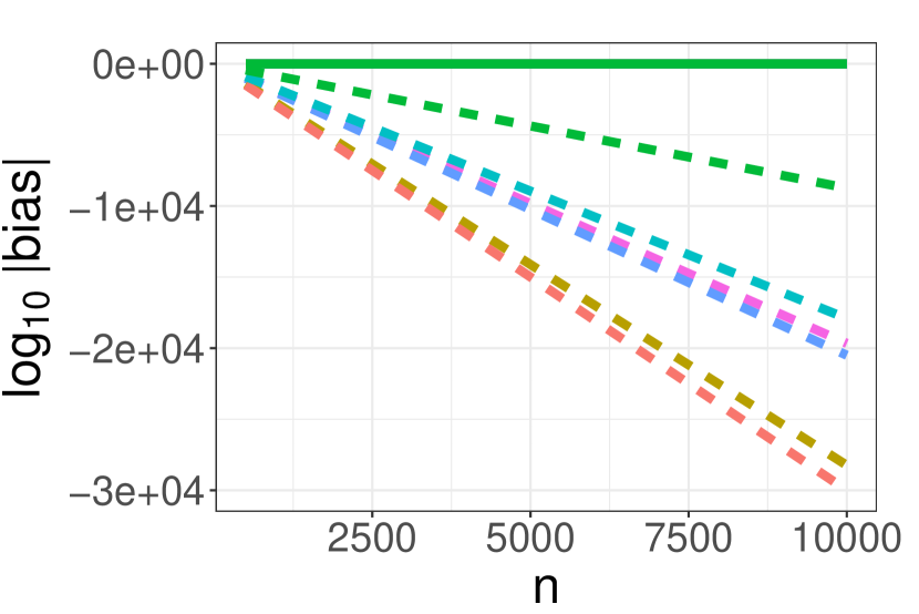
(a) $M_{0}$ ($S=1000$).

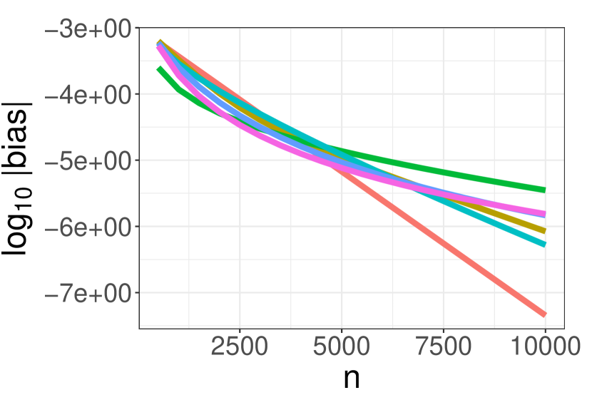
(b) $M_{0}$ ($S=1000$, cropped).

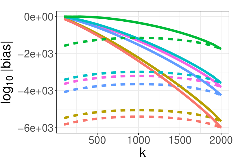
(c) $M_{k}$ ($S=1000$, $n=2000$).

$n$	$\hat{M}_{0}$	Bias	Var	MSE
100	GT	3.6973e-003	2.3372e-03	2.3508e-03
	ours	1.0000e-200	2.3515e-03	2.3515e-03
500	GT	6.6369e-005	1.1430e-05	1.1434e-05
	ours	$<$ 1.00e-200	1.1445e-05	1.1445e-05
1000	GT	4.3607e-007	4.3439e-08	4.3439e-08
	ours	$<$ 1.00e-200	4.3441e-08	4.3441e-08

(d) $M_{0}$ (uniform, $S=100$).

Figure 2: Results for our minimal-bias estimator $\hat{M}_{k}^{B}$. For our and baseline estimators, we show the logarithm of the absolute bias (a&b) as a function of $n$ for $k=0$ and (c) as a function of $k$ for $n=2000$. We also show (d) the bias, variance, and MSE of our and baseline estimator for three values of $n$. More plots can be found in Appendix E.

Since the underlying distribution $\{p_{x}\}_{x\in\mathcal{X}}$ is unknown, we can only estimate the MSE. For any element $x$ that has been observed exactly $k>0$ time in the sample $X^{n}$, we use $\hat{p}_{x}=\hat{M}_{k}^{G}/\Phi_{k}$ as natural estimator of $p_{x}$, where $\hat{M}_{k}^{G}$ is the GT estimator. To handle unobserved elements ($k=0$), we first estimate the number of unseen elements $\mathbb{E}\left[\Phi_{0}\right]=f_{0}(n)$ using Chao’s nonparamteric species richness estimator $\hat{f}_{0}=\frac{n-1}{n}\frac{\Phi_{1}^{2}}{2\Phi_{2}}$ (Chao, 1984), and then estimate the probability of each such unseen element as $\hat{p}_{y}=\hat{M}_{0}^{G}/\hat{f}_{0}$, where $\hat{M}_{0}^{G}$ is the GT estimator. Finally, we plug these estimates into Eqn. (15) to estimate the MSE. It is interesting to note that it is precisely the GT estimator whose MSE our approach is supposed to improve upon.

Genetic algorithm. With the required concepts in place, we are ready to introduce our genetic algorithm (GA) (Mitchell, 1998). Algorithm 1 sketches the general procedure. Given a target frequency $k$ (incl. $k=0$), the sample $X^{n}$, an iteration limit G, and the number $m$ of candidate representations to be mutated in every iteration, the algorithm produces an estimator $\hat{M}_{k}^{\text{Evo}}$ with minimal MSE.

Starting from the initial representation $r_{0}$ (Eqn. (10); Line 1), our GA iteratively improves a population of candidate representations $P_{g}$, called individuals. For every generation $g$ (Line 4), our GA selects the $m$ fittest individuals from the previous generation $P_{g-1}$ (Line 5), mutates them (Line 6), and creates the current generation $P_{g}$ by adding the initial representation $r_{0}$ and the Top-3 individuals from the previous generation (Line 7). The initial and previous Top-3 individuals are added to mitigate the risk of convergence to a local optimum. To mutate a representation $r$, our GA (i) chooses a random term $r$, (ii) applies Eqn. (11) where $\delta$ is chosen uniformly at random, (iii) applies a random identity from Eqn. (12–14), and (iv) adjusts the coefficients for the resulting representation $r^{\prime}$ accordingly. The iteration limit $G_{L}$ is increased if the current individuals do not improve on the initial individual $r_{0}$ or substantially improve on those discovered recently (Line 9–12).

Distribution-free. While our approach itself is distribution-free, the output is distribution-specific, i.e., the discovered estimator has a minimal MSE on the specific, unknown distribution. We explore this property in our experiments.

4 Experiment

We design experiments to evaluate the performance (i) of our minimal-bias estimator $\hat{M}_{k}^{B}$ and (ii) of our the minimal-MSE estimator $\hat{M}_{k}^{\text{Evo}}$ that is discovered by our genetic algorithm against the performance of the widely-used Good-Turing estimator $\hat{M}_{k}^{G}$ (Good, 1953).

Distibutions. We use the same six multinomial distributions that are used in previous evaluations (Orlitsky & Suresh, 2015; Orlitsky et al., 2016; Hao & Li, 2020): a uniform distribution (uniform), a half-and-half distribution where half of the elements have three times of the probability of the other half (half&half), two Zipf distributions with parameters $s=1$ and $s=0.5$ (zipf-1, zipf-0.5, respectively), and distributions generated by Dirichlet-1 prior and Dirichlet-0.5 prior (diri-1, diri-0.5, respectively).

Open Science and Replication. For scrutiny and replicability, we publish all our evaluation scripts at:

https://anonymous.4open.science/r/Better-Turing-157F.

4.1 Evaluating our Minimal-Bias Estimator

• RQ1. How does our estimator for the missing mass $\hat{M}_{0}^{B}$ compare to the Good-Turing estimator $\hat{M}_{0}^{G}$ in terms of bias as a function of sample size $n$?

• RQ2. How does our estimator for the total mass $\hat{M}_{k}^{B}$ compare to the Good-Turing estimator $\hat{M}_{k}^{G}$ in terms of bias as a function of frequency $k$?

• RQ3. How do the estimators compare in terms of variance and mean-squared error?

We focus specifically on the bias of $\hat{M}_{k}^{B}$, i.e., the average difference between the estimate and the expected value $\mathbb{E}\left[M_{k}\right]$. We expect that the bias of the missing mass estimate $\hat{M}_{0}^{B}$ as a function of $n$ across different distributions provides empirical insight for our claim that how much is unseen chiefly depends on information about the seen.

Table 1: The MSE of the best evolved estimator $M_{0}^{\text{Evo}}$ and GT estimator $\hat{M}_{0}^{G}$ for the missing mass $M_{0}$, the success rate $\hat{A}_{12}$, and the ratio (Ratio, $\mathit{MSE}(\hat{M}_{0}^{\text{Evo}})/\mathit{MSE}(M_{0}^{G})$) for three sample sizes $n$ and six distributions with support size $S=200$.

Dist.	$n=S/2$				$n=S$				$n=2S$
	$\mathit{MSE}(\hat{M}_{0}^{G})$	$\mathit{MSE}(M_{0}^{\text{Evo}})$	$\hat{A}_{12}$	Ratio	$\mathit{MSE}(\hat{M}_{0}^{G})$	$\mathit{MSE}(M_{0}^{\text{Evo}})$	$\hat{A}_{12}$	Ratio	$\mathit{MSE}(\hat{M}_{0}^{G})$	$\mathit{MSE}(M_{0}^{\text{Evo}})$	$\hat{A}_{12}$	Ratio
uniform	3.32e-03	2.04e-03	0.95	61%	1.17e-03	8.90e-04	0.99	76%	2.01e-04	1.70e-04	0.93	84%
half&half	3.33e-03	1.97e-03	0.96	59%	1.09e-03	8.58e-04	0.99	78%	2.11e-04	1.72e-04	1.00	81%
zipf-1	2.32e-03	2.41e-03	0.74	103%	8.16e-04	7.24e-04	0.88	88%	2.39e-04	2.11e-04	0.96	88%
zipf-0.5	3.23e-03	2.29e-03	0.89	71%	1.09e-03	8.52e-04	0.97	78%	2.30e-04	1.93e-04	1.00	83%
diri-1	2.99e-03	2.36e-03	0.85	78%	8.88e-04	6.65e-04	1.00	74%	1.96e-04	1.65e-04	0.96	84%
diri-0.5	2.55e-03	1.81e-03	0.94	71%	6.88e-04	4.86e-04	0.98	70%	1.61e-04	1.31e-04	0.93	81%
Avg.			0.88	74%			0.96	77%			0.96	84%

RQ.1. 2(a) illustrates how fast our estimator $\hat{M}_{k}^{B}$ and the baseline estimator $\hat{M}_{k}^{G}$ (GT) approach the expected missing mass $\mathbb{E}\left[M_{0}\right]$ as a function of sample size $n$. As it might difficult for the reader to discern differences across distributions for the baseline estimator, we refer to 2(b), where we zoom into a relevant region.

The magnitude of our estimator’s bias is significantly smaller than the magnitude of GT’s bias for all distributions (by thousands of orders of magnitude). Figure 2(a) also nicely illustrates the exponential decay of our estimator in terms of $n$ and how our estimator is less biased than GT by an exponential factor. In Figure 2(b), we can observe that GT’s bias also decays exponentially, although not nearly at the rate of our estimator.

In terms of distributions, a closer look at the performance differences confirms our suspicion that the bias of our estimator is strongly influenced by the probability $p_{\max}$ of the most abundant element while the bias of GT is strongly influenced by the probability $p_{\min}$ of the rarest element. In fact, by Eqn. (7) the absolute bias of our estimator is minimized when $p_{\max}$ is minimized. By Eqn. (6), GT’s bias is minimized if $p_{\min}$ is maximized. Since both is true for the uniform, both estimators exhibit the lowest bias for the uniform across all six distributions. GT performs similar on all distributions apart from the uniform (where bias seems minimal) and zipf-1 (where bias is maximized). For our estimator, if we ranked the distributions by values of $p_{\max}$ with the smallest value first $\langle\text{{\small{uniform}}, {\small{half\&half}}, {\small{zipf-0.5}}, {\small{zipf-1}}}\rangle$, we would arrive at the same ordering in terms of performance of our estimator as shown in 2(a).

RQ2. Figure 2(c) illustrates for both estimators of the total mass $M_{k}$ how the bias behaves as $k$ varies between $0$ and $n=2000$ when $S=1000$. The trend is clear; the bias of our estimator is strictly smaller than the bias of GT for all $k$ and all the distributions. The difference is the most significant for rare elements (small $k$) and gets smaller as $k$ increases. The bias of our estimator is maximized when $k=1000=0.5n$, the bias for GT when $k=0$.

RQ3. Table 2(d) shows variance and MSE of both estimators for the missing mass $M_{0}$ for the uniform and three values of $n$. As we can see, the MSE of our estimator is approximately the same as that of GT. The reason is that the MSE is dominated by the variance. We make the same observation for all other distributions (see Appendix E). The MSEs of both estimators are comparable.

4.2 Evaluating our Estimator Discovery Algorithm

• RQ1 (Effectiveness). How does our estimator for the missing mass $\hat{M}_{0}^{\text{Evo}}$ compare to the Good-Turing estimator $\hat{M}_{0}^{G}$ in terms of MSE?

• RQ2 (Efficiency). How long does it take for our genetic algorithm to generate an estimator $M_{k}^{\text{Evo}}$ given a sample?

• RQ3 (Distribution-awareness). How well does an estimator discovered from a sample from one distribution perform on another distribution in terms of MSE?

To handle the randomness in our evaluation, we repeat each experiment 100 times: 10 runs of the GA with 10 different samples $X^{n}$. More details about our experimental setup can be found in Appendix D.

RQ.1 (Effectiveness). Table 1 shows average MSE of the estimator $M_{0}^{\text{Evo}}$ discovered by our genetic algorithm and that of the GT estimator $\hat{M}_{0}^{G}$ for the missing mass $M_{0}$ across three sample sizes. We measure effect size using Vargha-Delaney $\hat{A}_{12}$ (Vargha & Delaney, 2000) (success rate), i.e., the probability that the MSE of the estimator discovered by our genetic algorithm has a smaller MSE than the GT estimator (larger is better). Moreover, we measure the MSE of our estimator as a proprtion of the MSE of GT, called ratio (smaller is better). Results for other support sizes $S$ can be found in Appendix E.

Overall, the estimator discovered by our GA performs significantly better than GT estimator in terms of MSE (avg. $\hat{A}_{12}>0.9$; $ratio<85\%$). The performance difference increases with sample size $n$. When the sample size is twice the support size ($n=2S$), in 96% of runs our discovered estimator performs better. The average MSE of our estimator is somewhere between 70% and 88% of the MSE of GT. The high success rate and the low ratio of the MSE shows that the GA is effective in finding the estimator with the minimal MSE for the missing mass $M_{0}$. A Wilcoxon signed-rank test shows that all performance differences are statistically significant at $\alpha<10^{-9}$.

In terms of distributions, the performance of our estimator is similar across all distributions, showing the generality of our algorithm. The only exception is the zipf-1, where the success rate is lower than for other distribution for $n=S/2$ and $S$, and the average ratio is 103% (yet, the median ratio is 85%) for $n=S/2$. The potential reason for this is due to the overfitting to the approximated distribution $\hat{p}_{x}$. Since the zipf-1 is the most skewed distribution, there are more elements unseen in the sample than in other distributions, which makes the approximated distribution $\hat{p}_{x}$ less accurate. Yet, the performance already improves and become similar to other distributions for $n=S$ and $n=2S$.

RQ.2 (Efficiency). The time it takes to discover the estimator is reasonable. To compute an estimator fo Table 1, it takes about seven (7) minutes on average and five (5) minutes on median. The average time for each iteration is 1.25s (median: 0.92).

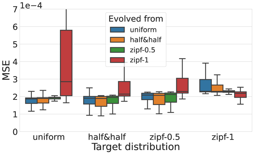
Figure 3: The MSE of an estimator discovered using a sample from one distribution (individual boxes) applied to another target distribution (clusters of boxes).

RQ.3 (Distribution-awareness). Figure 3 shows the performance of an estimator discovered from a sample from one distribution (source) when applied to another distribution (target). Applying an estimate from the zipf-1 on the zipf-1 gives the optimal MSE (right-most red box). However, applying an estimator from the zipf-1 on the uniform (left red box) yields a huge increase in variance. In terms of effect size, we measure a Vargha Delaney $\hat{A}_{12}>0.84$ between the “home” and “away” estimator. While each of the uniform and half&half also shows that the home estimator performs best on the home distribution ($\hat{A}_{12}=0.68$ (medium), $0.58$ (small), respectively), the difference between the estimators from uniform, half&half, and zipf-0.5 is less significant. Perhaps unsurprisingly, an estimator performs optimal when the source of the samples is similar to the target distribution.

Summary. To summarize, our GA is effective in finding the estimator with the minimal MSE for the missing mass $M_{0}$ with the smaller MSE than GT estimator $\hat{M}_{0}^{G}$ for all distributions and sample sizes. The effect is substantial and significant and the average decrease of the MSE is roughly one fifth against GT estimator $\hat{M}_{0}^{G}$.

5 Discussion

Beyond the General Estimator. In this study, we propose a meta-level estimation methodology that can be applied to a set of samples from a specific unknown distribution. The conventional approach is to develop an estimator for an arbitrary distribution. Yet, each distributions has its own characteristics, and, because of that, the manner of the (frequencies of) frequencies of the classes in the sample can be differ from, for example, the uniform distribution to the Zipf distribution. In contrast to the conventional approach, we propose a distribution-free methodology to discover the a distribution-specific estimator with low MSE (given only the sample). Note that, while we use the genetic algorithm to discover the estimator, any optimization method can be used to discover the estimator, for instance, a constrained optimization solver.

Extrapolating the Future Sampling. Estimating the number of unseen species is a well-known problem in many scientific fields, such as ecology, linguistics, and machine learning. Given $n$ samples, the expected number of hitherto unseen species that would be uncovered if $t$ times more samples were taken is $\mathbb{E}\left[U(t)\right]=f_{0}(n)-f_{0}(n+nt)$. Good & Toulmin (1956) proposed a seminal estimator using the frequencies of frequencies $\Phi_{k}$, similar to the Good-Turing estimator. Until recently, various subsequent studies have been conducted to improve the estimator (Efron & Thisted, 1976; Orlitsky et al., 2016; Hao & Li, 2020), while most of them still relies on the Poisson approximation to design the estimator. We believe that our analysis can be extended to the Good-Toulmin estimator seeking more accurate estimators for $U(t)$.

Appendix A Comparing the Bias of the Estimators

In Section 3.1, we have shown that the bias of a simpler variant of GT, $\hat{M}_{k}^{G^{\prime}}=\frac{k+1}{n-k}\Phi_{k+1}$, is larger by an exponential factor than the absolute bias of our minimal bias estimator $\hat{M}_{k}^{B}$. In this section, we show that the bias of the original GT estimator $\hat{M}_{k}^{G}=\frac{k+1}{n}\Phi_{k+1}$ is also larger by an exponential factor than the absolute bias of $\hat{M}_{k}^{B}$ for a sufficiently larger sample size. Recall that

$$\text{\emph{Bias}}_{G^{\prime}}=\mathbb{E}\left[\hat{M}_{k}^{G}-M_{k}\right]=\frac{k+1}{n-k}f_{k+1}(n)-{n\choose k}g_{k+1}(n+1)=\sum_{x}{n\choose k}p_{x}^{k+2}(1-p_{x})^{n-k-1},\\$$ (16)

and

$$\text{\emph{Bias}}_{G}=\mathbb{E}\left[\hat{M}_{k}^{G}-M_{k}\right] ={n\choose k}g_{k+2}(n+1)-\frac{k(k+1)}{n(n-k)}f_{k+1}(n)$$ (17)

$$={n\choose k}g_{k+2}(n+1)-\binom{n-1}{k-1}g_{k+1}(n)$$ (18)

$$=\sum_{x}p_{x}^{k+2}(1-p_{x})^{n-k-1}\left(\binom{n}{k}-\frac{1}{p_{x}}\cdot\binom{n-1}{k-1}\right)$$ (19)

$$=\sum_{x}\binom{n}{k}p_{x}^{k+2}(1-p_{x})^{n-k-1}\left(1-\frac{k}{n\cdot p_{x}}\right)$$ (20)

$$\geq\left(1-\frac{k}{n\cdot p_{\max}}\right)\text{\emph{Bias}}_{G^{\prime}},$$ (21)

where $1-\frac{k}{n\cdot p_{min}}>0$ when $n$ is sufficiently large. Above inequality leads to the following:

$$\frac{\text{\emph{Bias}}_{G}}{\text{\emph{Bias}}_{G^{\prime}}}\geq\left(1-\frac{k}{n\cdot p_{\max}}\right)\text{,}\quad\text{while}\quad\frac{\text{\emph{Bias}}_{B}}{\text{\emph{Bias}}_{G^{\prime}}}\leq\frac{Sp_{\max}^{k+2}}{p_{\min}^{k+2}}\left(\frac{1-p_{\min}}{p_{\max}}\right)^{-n+k+1},$$ (22)

which proves our claim.

Appendix B Bounding the Variance and the MSE of $\hat{M}_{k}^{B}$

The MSE of an estimator $\hat{e}$ for an estimand $e$ is defined as $MSE(\hat{e})=\mathbb{E}[(\hat{e}-e)^{2}]=\mathrm{Var}\left(\hat{e}\right)+\text{Bias}^{2}(\hat{e})$. As we have shown the bias of $\hat{M}_{k}^{B}$ in Section 3.1, the remaining part to compute the MSE of $\hat{M}_{k}^{B}$ is to compute its variance.

The variance of the linear combination of random variables is given by

$$\mathrm{Var}\left(\sum_{i}c_{i}X_{i}\right)=\sum_{i}c_{i}^{2}\mathrm{Var}\left(X_{i}\right)+\sum_{i\neq j}c_{i}c_{j}\mathrm{Cov}\left(X_{i},X_{j}\right).$$ (23)

Therefore, the variance and the covariance of $\Phi_{i}(n)$s are the missing pieces to compute the variance of $\hat{M}_{k}^{B}$.

Theorem B.1.

Given the multinomial distribution $p=(p_{1},\dots,p_{S})$ with support size $S$, the variance of $\Phi_{i}=\Phi_{i}(n)$ from $n$ samples $X^{n}$ is given by

$$\mathrm{Var}\left(\Phi_{i}(n)\right)=\begin{cases}f_{i}(n)-f_{i}(n)^{2}+\sum_{x\neq y}\frac{n!}{i!^{2}(n-2i)!}p_{x}^{i}p_{y}^{i}(1-p_{x}-p_{y})^{n-2i}&\text{if $2i\leq n$,}\\ f_{i}(n)-f_{i}(n)^{2}&\text{otherwise.}\end{cases}$$ (24)

Proof.

$$\mathrm{Var}\left(\Phi_{i}\right) =\mathbb{E}\left[\Phi_{i}^{2}\right]-\mathbb{E}\left[\Phi_{i}\right]^{2}$$ (25)

$$\mathbb{E}\left[\Phi_{i}^{2}\right] =\mathbb{E}\left[\left(\sum_{x}\mathbbm{1}(N_{x}=i)\right)^{2}\right]$$ (26)

$$=\mathbb{E}\left[\sum_{x}\mathbbm{1}(N_{x}=i)+\sum_{x\neq y}\mathbbm{1}(N_{x}=i\land N_{y}=i)\right]$$ (27)

$$=\begin{cases}f_{i}(n)+\sum_{x\neq y}\frac{n!}{i!^{2}(n-2i)!}p_{x}^{i}p_{y}^{i}(1-p_{x}-p_{y})^{n-2i}&\text{if $2i\leq n$,}\\ f_{i}(n)&\text{otherwise.}\end{cases}$$ (28)

$$\therefore\mathrm{Var}\left(\Phi_{i}\right) =\begin{cases}f_{i}(n)+\sum_{x\neq y}\frac{n!}{i!^{2}(n-2i)!}p_{x}^{i}p_{y}^{i}(1-p_{x}-p_{y})^{n-2i}-f_{i}(n)^{2}&\text{if $2i\leq n$,}\\ f_{i}(n)-f_{i}(n)^{2}&\text{otherwise.}\end{cases}$$ (29)

∎

Now we compute the upper bound of the variance of $\hat{M}_{k}^{B}$.

Lemma B.2.

$$\mathrm{Var}\left(\Phi_{i}\right)\begin{cases}\leq Sf_{i}(n)-f_{i}(n)^{2}&\text{if $2i\leq n$.}\\ =f_{i}(n)-f_{i}(n)^{2}&\text{otherwise.}\end{cases}$$ (30)

Proof.

From Theorem B.1,

$$\mathbb{E}\left[\Phi_{i}^{2}\right] =f_{i}(n)+\mathbb{E}\left[\sum_{x\neq y}\mathbbm{1}(N_{x}=i\land N_{y}=i)\right]$$ (31)

$$\leq f_{i}(n)+(S-1)\mathbb{E}\left[\sum_{x}\mathbbm{1}(N_{x}=i)\right]$$ (32)

$$=Sf_{i}(n)\quad\text{(if $2i\leq n$)}.$$ (33)

The lemma directly follows from the above inequality. ∎

Lemma B.3.

$$g_{i}(n)\leq S\cdot\beta_{\min}^{-n}o_{\max}^{i},$$

where $S=|\mathcal{X}|$, $p_{\max}=\max_{x\in\mathcal{X}}p_{x}$, $\beta_{\min}=\frac{1}{1-p_{\min}}$, and $o_{\max}=\frac{p_{\max}}{1-p_{\max}}$.

Proof.

$\frac{1}{1-x}$ and $\frac{x}{1-x}$ are increasing functions for $x\in(0,1)$. Therefore,

$$g_{i}(n)=\sum_{x\in\mathcal{X}}p_{x}^{i}(1-p_{x})^{n-i}=\sum_{x\in\mathcal{X}}\left(\frac{1}{1-p_{x}}\right)^{-n}\left(\frac{p_{x}}{1-p_{x}}\right)^{i}\leq|\mathcal{X}|\cdot\beta_{\min}^{-n}o_{\max}^{i}.$$

∎

Theorem B.4.

The variance of the estimator $\hat{M}_{k}^{B}$ is bounded as follows:

$$\mathrm{Var}(\hat{M}_{k}^{B})\leq c_{1}\cdot n^{2k+1}\cdot c_{2}^{-n},$$

where $c_{1}=S\cdot\left(\frac{e}{k}\right)^{2k}$, $c_{2}=\min\left(\frac{1}{1-p_{\min}},\frac{1-p_{\max}}{p_{\max}(1-p_{\min})}\right)$. In other words, $\mathrm{Var}(\hat{M}_{k}^{B})=\mathcal{O}(n^{2k+1}\cdot\beta_{\min}^{-n}\cdot\max(1,o_{\max}^{n}))$.

Proof.

From Lemma B.2 in the supplementary, we have $\mathrm{Var}(\Phi_{i})\leq Sf_{i}(n)-f_{i}(n)^{2}$. Thus,

$$\mathrm{Var}\left(\frac{\Phi_{k+i}}{\binom{n}{k+i}}\right) \leq\frac{Sf_{k+i}(n)-f_{k+i}(n)^{2}}{\binom{n}{k+i}^{2}}\leq S\cdot\frac{g_{k+i}(n)}{\binom{n}{k+i}}\leq\frac{S^{2}\cdot\beta_{\min}^{-n}o_{\max}^{k+i}}{\binom{n}{k+1}}\quad\text{(by Lemma~{}\ref{lemma:bound})}$$

$$\binom{n}{k}^{2}\mathrm{Var}\left(\frac{\Phi_{k+i}}{\binom{n}{k+i}}\right) \leq S\beta_{\min}^{-n}\frac{\binom{n}{k}^{2}}{\binom{n}{k+1}}o_{\max}^{k+i}\leq S\beta_{\min}^{-n}\frac{\left(\frac{e^{2}n^{2}}{k^{2}}\right)^{k}}{\left(\frac{n}{k+i}\right)^{k}}o_{\max}^{k+i}\leq S\beta_{\min}^{-n}\left(\frac{e^{2}n(k+i)}{k^{2}}\right)^{k}o_{\max}^{k+i}$$

$$\leq S\beta_{\min}^{-n}\left(\frac{e^{2}n^{2}}{k^{2}}\right)^{k}O_{M}=S\beta_{\min}^{-n}\left(\frac{en}{k}\right)^{2k}O_{M},\quad\text{where }O_{M}=\max(o_{\max}^{k},o_{\max}^{n}),$$

$$\mathrm{Var}(\hat{M}_{k}^{B}) =\binom{n}{k}^{2}\mathrm{Var}\left(\sum_{i=1}^{n-k}(-1)^{i-1}\frac{\Phi_{k+1}}{\binom{n}{k+1}}\right)$$

$$\leq(n-k)\binom{n}{k}^{2}\mathrm{Var}\left(\frac{\Phi_{k+1}}{\binom{n}{k+1}}\right)$$ (35)

$$\leq S(n-k)\left(\frac{en}{k}\right)^{2k}\cdot\beta_{\min}^{-n}O_{M}=\mathcal{O}(n^{2k+1})\cdot\beta_{\min}^{-n}O_{M},$$

where (35) follows from Cauchy-Schwarz inequality ($\mathrm{Var}(\sum_{j=1}^{M}X_{i})\leq M\cdot\sum_{j=1}^{M}\mathrm{Var}(X_{i})$). The proof follows from dividing the variance of the estimator into two cases: $o_{\max}<1$ and $o_{\max}>1$: If $o_{\max}<1$, $O_{M}=o_{\max}^{k}$, and $\mathrm{Var}(\hat{M}_{k}^{B})=\mathcal{O}(n^{2k+1}\beta_{\min}^{-n})$. If $o_{\max}>1$, $O_{M}=o_{\max}^{n}$, and, $\mathrm{Var}(\hat{M}_{k}^{B})=\mathcal{O}(n^{2k+1}\beta_{\min}^{-n}o_{\max}^{n})$. ∎

Therefore, the variance exponentially decreases with $n$ if $p_{\max}<0.5$ or $\frac{1-p_{\max}}{p_{\max}(1-p_{\min})}<1$.

Corollary B.5.

There exists a constant $c>1$ such that

$$\mathrm{MSE}(\hat{M}_{k}^{B})\leq\mathcal{O}(n^{2k+1}c^{-n}).$$

Proof.

From Equ. (7) in the manuscript, the bias $|\mathbb{E}(\hat{M}_{k}^{B})-M_{k}|\leq S\cdot p_{\max}\cdot n^{k}\cdot p_{\max}^{n}$. The proof follows from the fact that $\mathrm{MSE}=\mathrm{Var}+\mathrm{Bias}^{2}$ and the bound of the variance and the bias. ∎

Appendix C Computing the Variance and the MSE of the Evolved Estimators

Same as $\hat{M}_{k}^{B}$, the evolved estimators from the genetic algorithm are also linear combinations of $\Phi_{k}(n)$s (while varying both $k$ and $n$ unlike $\hat{M}_{k}^{B}$). Given the evolved estimator $\hat{M}_{k}^{\text{Evo}}=\sum_{i}c_{i}\Phi_{k_{i}}(n_{i})$, the expected value of $\hat{M}_{k}^{\text{Evo}}$ is given by substituting $\Phi_{k}(n)$ with $f_{k}(n)$:

$$\mathbb{E}(\hat{M}_{k}^{\text{Evo}})=\sum_{i}c_{i}f_{k_{i}}(n_{i}).$$ (36)

Given the multinomial distribution $p$, the covariance between $\Phi_{k}(n)$ and $\Phi_{k^{\prime}}(n^{\prime})$, which is needed to compute the variance of $\hat{M}_{k}^{\text{Evo}}$ as Equ. (23), can be computed as follows:

Theorem C.1.

Given the multinomial distribution $p=(p_{1},\dots,p_{S})$ with support size $S$, let $X^{n_{total}}$ be the set of $n_{total}$ samples from $p$. Let $X^{n}$ and $X^{n^{\prime}}$ be the first $n$ and $n^{\prime}$ samples from $X^{n_{total}}$, respectively; WLOG, we assume $1\leq n^{\prime}\leq n\leq n_{total}$. Then, the covariance of $\Phi_{k}(n)=\Phi_{k}(X^{n})$ and $\Phi_{k^{\prime}}(n^{\prime})=\Phi_{k^{\prime}}(X^{n^{\prime}})$ ($1\leq k\leq n$, $1\leq k^{\prime}\leq n^{\prime}$) is given by following:

$$\mathrm{Cov}\left(\Phi_{k}(n),\Phi_{k^{\prime}}(n^{\prime})\right) =\mathbb{E}\left[\Phi_{k}(n)\cdot\Phi_{k^{\prime}}(n^{\prime})\right]-f_{k}(n)\cdot f_{k^{\prime}}(n^{\prime})$$ (37)

$$=\mathbb{E}\left[\left(\sum_{x}\mathbbm{1}(N_{x}=k)\right)\cdot\left(\sum_{x^{\prime}}\mathbbm{1}({N^{\prime}}_{x^{\prime}}=k^{\prime})\right)\right]-f_{k}(n)\cdot f_{k^{\prime}}(n^{\prime})$$ (38)

$$=\sum_{x}\sum_{x^{\prime}}\mathbb{E}\left[\mathbbm{1}(N_{x}=k\land{N^{\prime}}_{x^{\prime}}=k^{\prime})\right]-f_{k}(n)\cdot f_{k^{\prime}}(n^{\prime}),$$ (39)

where ${N^{\prime}}_{x^{\prime}}$ is the number of occurrences of $x^{\prime}$ in $X^{n^{\prime}}$. Depending on the values of $n,n^{\prime},k,k^{\prime},x,$ and $x^{\prime}$, the $\mathbb{E}\left[\mathbbm{1}(N_{x}=k\land{N^{\prime}}_{x^{\prime}}=k^{\prime})\right]$ can be computed as follows:

$\forall n,n^{\prime}$ s.t.	$\forall x,x^{\prime}$ s.t.	$\forall k,k^{\prime}$ s.t.	$\mathbb{E}\left[\mathbbm{1}(N_{x}=k\land{N^{\prime}}_{x^{\prime}}=k^{\prime})\right]$
$n=n^{\prime}$	$x=x^{\prime}$	$k=k^{\prime}$	$\binom{n}{k}p_{x}^{k}(1-p_{x})^{n-k}$
		$k\neq k^{\prime}$	$0$ (infeasible)
	$x\neq x^{\prime}$	$k+k^{\prime}\leq n$	$\frac{n!}{k!k^{\prime}!(n-k-k^{\prime})!}p_{x}^{k}p_{x^{\prime}}^{k^{\prime}}(1-p_{x}-p_{x^{\prime}})^{n-k-k^{\prime}}$
		$k+k^{\prime}>n$	$0$ (infeasible)
$n\neq n^{\prime}$	$x=x^{\prime}$	$k^{\prime}\leq k$	$\binom{n^{\prime}}{k^{\prime}}p_{x}^{k^{\prime}}(1-p_{x})^{n^{\prime}-k^{\prime}}\cdot\binom{n-n^{\prime}}{k-k^{\prime}}p_{x}^{k-k^{\prime}}(1-p_{x})^{(n-n^{\prime})-(k-k^{\prime})}$
		$k^{\prime}>k$	$0$ (infeasible)
	$x\neq x^{\prime}$	$k+k^{\prime}\leq n$	$\sum_{i=\max(0,k-(n-n^{\prime}))}^{\min(k,n-k^{\prime})}\frac{n^{\prime}!}{k^{\prime}!i!(n^{\prime}-k^{\prime}-i)!}\frac{(n-n^{\prime})!}{(k-i)!((n-n^{\prime})-(k-i))!}p_{x^{\prime}}^{k^{\prime}}p_{x^{\prime}}^{k^{\prime}}(1-p_{x}-p_{x^{\prime}})^{n^{\prime}-k^{\prime}-i}p_{x}^{k}(1-p_{x})^{(n-n^{\prime})-(k-i)}$
		$k+k^{\prime}>n$	$0$ (infeasible)

Proof.

The proof is straightforward from the definition of $N_{x}$ and ${N^{\prime}}_{x^{\prime}}$. ∎

Given the expected value and the variance of $\hat{M}_{k}^{\text{Evo}}$, the MSE of $\hat{M}_{k}^{\text{Evo}}$ naturally follows.

Appendix D Details of the Hyperparameters of the Evolutionary Algorithm

For evaluating Algorithm 1, we use the following hyperparameters:

• Same as the Orlitsky’s study (Orlitsky & Suresh, 2015), which assess the performance of the Good-Turing estimator, we use the hybrid estimator $\hat{p}$ of the empirical estimate and the Good-Turing estimate to approximate the underlying distribution $\{p_{x}\}_{x\in\mathcal{X}}$ for estimating the MSE of the evolved estimator. The hybrid estimator $\hat{p}$ is defined as follows: If $N_{x}=k$,

  $$\hat{p}_{x}=\begin{cases}c\cdot\frac{k}{N}&\text{if }k<\Phi_{k+1},\\ c\cdot\frac{\hat{M}_{k}^{G}}{\Phi_{k}}&\text{otherwise,}\end{cases}$$

  where $c$ is a normalization constant such that $\sum_{x\in\mathcal{X}}\hat{p}_{x}=1$.

• The number of generations $G=100$. To avoid the algorithm from converging to a local minimum, we limit the maximum number of generations to be $2000$.

• The mutant size $m=40$.

• When selecting the individuals for the mutation, we use tournament selection with tournament size $t=3$, i.e., we randomly choose three individuals with replacement and select the best one, and repeat this process $m$ times.

• When choosing the top three individuals when constructing the next generation, we use elitist selection, i.e., choosing the top three individuals with the smallest fitness values.

• To avoid the estimator from being too complex, we limit the maximum number of terms in the estimator to be $20$.

The actual script implementing Algorithm 1 can be found at the publically available repository

https://anonymous.4open.science/r/Better-Turing-157F.

Appendix E Additional Experimental Results

Table 2: The MSE of the Good-Turing estimator $\hat{M}_{0}^{G}$, minimal bias estimator $\hat{M}_{0}^{B}$, and the best evolved estimator $\hat{M}_{0}^{\text{Evo}}$ and for the missing mass $M_{0}$, the success rate $\hat{A}_{12}$ of the evolved estimator ($X_{2}$) against the Good-Turing estimator ($X_{1}$), and the ratio (Ratio, $\mathit{MSE}(M_{0}^{\text{Evo}})/\mathit{MSE}(\hat{M}_{0}^{G})$) for two support sizes $S=100$ and $200$, three sample sizes $n$ and six distributions.

$S$	$n/S$	Distribution	$\mathit{MSE}(\hat{M}_{0}^{B})$	$\mathit{MSE}(\hat{M}_{0}^{G})$	$\mathit{MSE}(\hat{M}_{0}^{\text{evo}})$	$\hat{A}_{12}$	Ratio
100	0.5	uniform	6.834e-03	6.681e-03	6.267e-03	62%	93%
		half&half	6.821e-03	6.694e-03	4.489e-03	85%	67%
		zipf-0.5	6.676e-03	6.565e-03	3.311e-03	94%	50%
		zipf-1	4.995e-03	4.943e-03	3.065e-03	98%	62%
		diri-1	6.166e-03	6.086e-03	3.202e-03	96%	52%
		diri-0.5	5.223e-03	5.167e-03	2.708e-03	100%	52%
	1.0	uniform	2.365e-03	2.351e-03	1.905e-03	88%	81%
		half&half	2.200e-03	2.190e-03	1.439e-03	97%	65%
		zipf-0.5	2.207e-03	2.194e-03	1.982e-03	75%	90%
		zipf-1	1.713e-03	1.704e-03	1.705e-03	75%	100%
		diri-1	1.787e-03	1.778e-03	1.066e-03	100%	60%
		diri-0.5	1.388e-03	1.381e-03	8.747e-04	97%	63%
	2.0	uniform	4.047e-04	4.028e-04	3.428e-04	89%	85%
		half&half	4.237e-04	4.221e-04	3.035e-04	97%	71%
		zipf-0.5	4.580e-04	4.561e-04	3.321e-04	95%	72%
		zipf-1	4.826e-04	4.810e-04	3.633e-04	98%	75%
		diri-1	3.946e-04	3.932e-04	2.473e-04	100%	62%
		diri-0.5	3.276e-04	3.264e-04	2.587e-04	87%	79%
200	0.5	uniform	3.361e-03	3.323e-03	2.044e-03	95%	61%
		half&half	3.357e-03	3.326e-03	1.968e-03	96%	59%
		zipf-0.5	3.254e-03	3.227e-03	2.293e-03	89%	71%
		zipf-1	2.335e-03	2.324e-03	2.410e-03	74%	103%
		diri-1	3.011e-03	2.992e-03	2.359e-03	85%	78%
		diri-0.5	2.563e-03	2.550e-03	1.813e-03	94%	71%
	1.0	uniform	1.172e-03	1.169e-03	8.900e-04	99%	76%
		half&half	1.092e-03	1.090e-03	8.584e-04	99%	78%
		zipf-0.5	1.091e-03	1.088e-03	8.525e-04	97%	78%
		zipf-1	8.185e-04	8.165e-04	7.244e-04	88%	88%
		diri-1	8.898e-04	8.876e-04	6.652e-04	100%	74%
		diri-0.5	6.900e-04	6.882e-04	4.861e-04	98%	70%
	2.0	uniform	2.017e-04	2.012e-04	1.702e-04	93%	84%
		half&half	2.113e-04	2.109e-04	1.716e-04	100%	81%
		zipf-0.5	2.307e-04	2.302e-04	1.929e-04	100%	83%
		zipf-1	2.390e-04	2.387e-04	2.109e-04	96%	88%
		diri-1	1.961e-04	1.958e-04	1.648e-04	96%	84%
		diri-0.5	1.609e-04	1.607e-04	1.315e-04	93%	81%

References

• Acharya et al. (2013) Acharya, J., Jafarpour, A., Orlitsky, A., and Suresh, A. T. Optimal probability estimation with applications to prediction and classification. In Shalev-Shwartz, S. and Steinwart, I. (eds.), Proceedings of the 26th Annual Conference on Learning Theory, volume 30 of Proceedings of Machine Learning Research, pp.  764–796, Princeton, NJ, USA, 12–14 Jun 2013. PMLR.
• Chao (1984) Chao, A. Nonparametric estimation of the number of classes in a population. Scandinavian Journal of statistics, pp.  265–270, 1984.
• Chao & Jost (2012) Chao, A. and Jost, L. Coverage-based rarefaction and extrapolation: standardizing samples by completeness rather than size. Ecology, 93 12:2533–47, 2012.
• Drukh & Mansour (2004) Drukh, E. and Mansour, Y. Concentration bounds for unigrams language model. In Shawe-Taylor, J. and Singer, Y. (eds.), Learning Theory, pp.  170–185, Berlin, Heidelberg, 2004. Springer Berlin Heidelberg. ISBN 978-3-540-27819-1.
• Efron & Thisted (1976) Efron, B. and Thisted, R. Estimating the number of unsen species: How many words did shakespeare know? Biometrika, 63(3):435–447, 1976. ISSN 00063444. URL http://www.jstor.org/stable/2335721.
• Good (1953) Good, I. J. The population frequencies of species and the estimation of population parameters. Biometrika, 40(3-4):237–264, 1953.
• Good & Toulmin (1956) Good, I. J. and Toulmin, G. H. The number of new species, and the increase in population coverage, when a sample is increased. Biometrika, 43(1/2):45–63, 1956. ISSN 00063444. URL http://www.jstor.org/stable/2333577.
• Hao & Li (2020) Hao, Y. and Li, P. Optimal prediction of the number of unseen species with multiplicity. In Larochelle, H., Ranzato, M., Hadsell, R., Balcan, M., and Lin, H. (eds.), Advances in Neural Information Processing Systems, volume 33, pp.  8553–8564. Curran Associates, Inc., 2020. URL https://proceedings.neurips.cc/paper/2020/file/618790ae971abb5610b16c826fb72d01-Paper.pdf.
• Juang & Lo (1994) Juang, B.-H. and Lo, S. On the bias of the turing-good estimate of probabilities. IEEE Transactions on signal processing, 2(42):496–498, 1994.
• McAllester & Schapire (2000) McAllester, D. and Schapire, R. E. On the convergence rate of good-Turing estimators. In Proceedings of the 13th Annual Conference on Computational Learning Theory, pp.  1–6. Morgan Kaufmann, San Francisco, 2000.
• Mitchell (1998) Mitchell, M. An introduction to genetic algorithms. MIT press, 1998.
• Orlitsky & Suresh (2015) Orlitsky, A. and Suresh, A. T. Competitive distribution estimation: Why is good-turing good. In Cortes, C., Lawrence, N., Lee, D., Sugiyama, M., and Garnett, R. (eds.), Advances in Neural Information Processing Systems, volume 28. Curran Associates, Inc., 2015. URL https://proceedings.neurips.cc/paper/2015/file/d759175de8ea5b1d9a2660e45554894f-Paper.pdf.
• Orlitsky et al. (2003) Orlitsky, A., Santhanam, N. P., and Zhang, J. Always good turing: Asymptotically optimal probability estimation. Science, 302(5644):427–431, 2003. doi: 10.1126/science.1088284.
• Orlitsky et al. (2016) Orlitsky, A., Suresh, A. T., and Wu, Y. Optimal prediction of the number of unseen species. Proceedings of the National Academy of Sciences, 113(47):13283–13288, 2016. doi: 10.1073/pnas.1607774113. URL https://www.pnas.org/doi/abs/10.1073/pnas.1607774113.
• Painsky (2022) Painsky, A. Convergence guarantees for the good-turing estimator. Journal of Machine Learning Research, 23(279):1–37, 2022. URL http://jmlr.org/papers/v23/21-1528.html.
• Valiant & Valiant (2016) Valiant, G. and Valiant, P. Instance optimal learning of discrete distributions. In Proceedings of the Forty-Eighth Annual ACM Symposium on Theory of Computing, STOC ’16, pp.  142–155, New York, NY, USA, 2016. Association for Computing Machinery. ISBN 9781450341325. doi: 10.1145/2897518.2897641. URL https://doi.org/10.1145/2897518.2897641.
• Vargha & Delaney (2000) Vargha, A. and Delaney, H. D. A critique and improvement of the cl common language effect size statistics of mcgraw and wong. Journal of Educational and Behavioral Statistics, 25(2):101–132, 2000.