Sparse-VQ Transformer: An FFN-Free Framework with Vector Quantization for Enhanced Time Series Forecasting

Abstract.

Time series analysis is vital for numerous applications, and transformers have become increasingly prominent in this domain. Leading methods customize the transformer architecture from NLP and CV, utilizing a patching technique to convert continuous signals into segments. Yet, time series data are uniquely challenging due to significant distribution shifts and intrinsic noise levels. To address these two challenges, we introduce the Sparse Vector Quantized FFN-Free Transformer (Sparse-VQ). Our methodology capitalizes on a sparse vector quantization technique coupled with Reverse Instance Normalization (RevIN) to reduce noise impact and capture sufficient statistics for forecasting, serving as an alternative to the Feed-Forward layer (FFN) in the transformer architecture. Our FFN-free approach trims the parameter count, enhancing computational efficiency and reducing overfitting. Through evaluations across ten benchmark datasets, including the newly introduced CAISO dataset, Sparse-VQ surpasses leading models with a 7.84% and 4.17% decrease in MAE for univariate and multivariate time series forecasting, respectively. Moreover, it can be seamlessly integrated with existing transformer-based models to elevate their performance. Our source code and the new dataset are available at: https://anonymous.4open.science/r/Sparse-VQ-DC28.

1. Introduction

Time series forecasting involves making predictions based on historical data, which is widely used in various real-world applications including weather forecasting, stock prediction, energy consumption planning, E-commerce supply chain scheduling, etc. With the evolution of deep learning techniques, traditional statistical approaches (Box and Jenkins, 1968; Hyndman and Athanasopoulos, 2018; Salinas et al., 2020; Taylor and Letham, 2018) have been largely superseded by deep learning models (Bai et al., 2018; Qin et al., 2017). More recently, the success of Transformers in the NLP and CV domain (Vaswani et al., 2017; Devlin et al., 2019; Dosovitskiy et al., 2021; Rao et al., 2021) has led to their adoption in time series forecasting tasks and yielded promising results, making a significant shift in the techniques employed for predictive analytics.

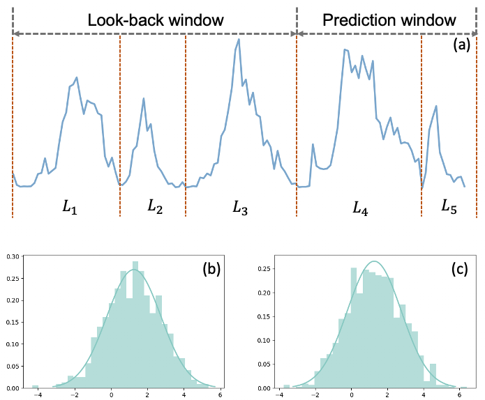
Figure 1. Although the temporal covariate shift problem exists in non-stationary time series, as shown in (a), historical patterns may still reoccur in the future. For example, the distribution of $L_{2}$ (b) are similar to that of $L_{5}$ (c).

However, a significant portion of time series data generated in real-world scenarios inherently exhibits non-stationary property. This suggests that statistical features, including low-order statistics like the mean and variance, as well as high-order statistics encompassing higher moments, often experience variations over time, a phenomenon referred to as distribution shift (Fan et al., 2023). This issue often leads to poor generalization, posing significant challenges in time series forecasting. Previous studies (Passalis et al., 2019; Ogasawara et al., 2010; Fan et al., 2023) focused on applying normalization as a pre-processing technique for time series prediction, which mitigates the non-stationarity of the raw time series and offers a relatively stable data distribution for models, resulting in improved predictability. Building on these, RevIN (Kim et al., 2022) proposed to restore the low-order statistical information of a time-series instance and implement the reversible normalization after the model output, which has been proven powerful and used extensively. Another common challenge encountered in time series analysis is the presence of high noise or low signal density. When the vanilla transformer model is applied to individual time points, its performance tends to be unsatisfactory. Recent studies showed that this issue can be mitigated by employing a straightforward patching technique to tokenize the signal, thereby enhancing its representation (Nie et al., 2022; Lin et al., 2023).

Transformers have made significant strides in NLP and image recognition, with applications such as ChatGPT and Midjourney showcasing their capabilities. Studies reveal that a single attention layer in transformers can be seen as a compound of bigram and "skip-trigram" (patterns like "A… B C") configurations. Each attention head can deftly navigate from a given token ("B") to an antecedent one ("A"), influencing the likelihood of a successive token ("C")—a key engineering feat driving transformer success. Furthermore, the Feed-Forward Network (FFN) module serves as a conceptual archive, encoding token co-occurrences (A, B, C)—indicative of high-order statistics (Geva et al., 2020, 2021a; Dai et al., 2022).

In contrast, time series data are sequential numerical recordings, distinct from NLP tokens or vision patches. Reliable extraction of statistical features from noisy time series is crucial for accurate forecasting. However, FFNs encounter limitations in modeling simple polynomial relationships (e.g., $x_{i}*x_{j}$) due to MLPs’ inherent approximation challenges (Tao et al., 2020). Consequently, it remains an open question whether the conventional FFN-plus-attention architecture of transformers is optimal for time series forecasting.

Given that time series data often exhibit drift in data distribution, we expect a significant change over time in low-order statistics mean, variance and high order statistics, a less desirable case for the usage of the FFN module. In our study, we develop a hybrid approach, dubbed Sparse-VQ, that can better capture statistics of drifting distributions than the FFN module: we first apply Reversible Instance Normalization (RevIN) to directly model local low-order statistics, specifically the mean and variance, and then employ vector quantization to reduce noise from inputs and capture global statistics. Our extensive empirical studies show that Sparse-VQ can substantially improve the prediction performance for non-stationary and noisy signals over the FFN module, leading to what we call FFN-free transformer for time series forecasting. This FFN-free approach significantly reduces the model’s parameter count, leading to an significant improvement in computation and improved generalization.

Here we summarize our key contributions as follows:

1. We propose the Sparse-VQ structure that embeds long time series into a discrete space, thus effectively reducing the impact of noise from the data.

2. We investigate the effect of FFN structure in Transformer and propose a FFN-free Transformer structure that can achieve a remarkable 21.52% reduction in parameters with improved performance.

3. We have conducted extensive experiments on ten diverse benchmark datasets, including the novel CAISO dataset, and the periodic Traffic dataset, which is ideal for testing forecasting periodic time series. Our empirical studies show that compared with state-of-the-art methods, Sparse-VQ can reduce the prediction error by 4.17% and 7.84% for multivariate and univariate forecasting, respectively. Also, our empirical findings show that the proposed framework has the potential to substantially enhance the performance of all Tranformer-based models.

The remainder of this paper is structured as follows: In Section 2, we provide a summary of related work. Section 4 presents the detailed framework designed for our proposed approach and introduces the Sparse-VQ and FFN-free Transformer structure. In Section 5, we conduct the numerical experiments to evaluate the performance of our proposed method in long-time, short-time and few-shot forecasting tasks compared to various SOTA baseline models. Furthermore, we present ablation experiments, boosting results of Sparse-VQ, different variants of Vector Quantization and robustness studies. Finally, in Section  6, the conclusions and future research directions are discussed.

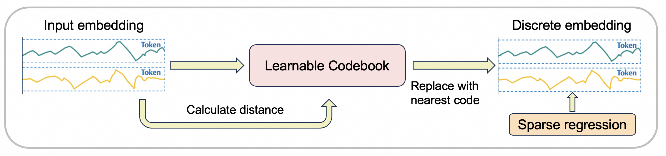
Figure 2. Sparse-VQ Block(SVQ).

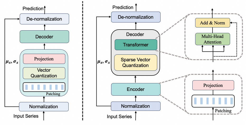
Figure 3. Classic model with incorporation of VQ(left) and Sparse-VQ Model Overview(right).

2. Related Work

Here we present a concise summary of related work on time series forecasting, distribution shift, and vector quantization. For a more detailed review, please refer to Appendix A.

2.1. Time Series Forecasting

Time series forecasting has progressed from traditional statistical algorithms like ARIMA (Box and Jenkins, 1968) and Holt-Winter (Hyndman and Athanasopoulos, 2018) to machine learning models including DeepAR (Salinas et al., 2020) and Prophet (Taylor and Letham, 2018). The advent of deep learning has led to the adoption of sophisticated neural networks such as TCN (Bai et al., 2018) and LSTM (Hochreiter and Schmidhuber, 1997), with notable contributions from N-BEATS (Oreshkin et al., 2019), which excelled in the M4 competition. Transformer-based models, including Informer (Zhou et al., 2021), Reformer (Kitaev et al., 2020), and Autoformer (Wu et al., 2021), have significantly improved time series forecasting. Innovations like TimesNet (Wu et al., 2022), FiLM (Zhou et al., 2022b), FEDformer (Zhou et al., 2022a), and Pyraformer (Liu et al., 2022) continue to refine these techniques. Pretrained models such as FPT (Zhou et al., 2023) showcase the adaptability of language or vision models to time series tasks, cementing Transformer-based methods as a top-tier approach (Wen et al., 2022; Shao et al., 2023).

2.2. Distribution Shift

Addressing distribution shifts in non-stationary time series data is a persistent challenge. To tackle this issue, researchers mainly utilize domain adaptation (Tzeng et al., 2017; Ganin et al., 2016; Wang et al., 2018) and generalization strategies (Wang et al., 2021; Li et al., 2018; Muandet et al., 2013; Lu et al., 2022) to mitigate the distribution shift. Adaptive RNNs (Du et al., 2021), RevIN (Kim et al., 2021), and DIVERSIFY (Lu et al., 2023) have emerged as novel solutions, leveraging period segmentation, normalization techniques, and out-of-distribution learning to cope with varying distributions.

2.3. Vector Quantization

Vector quantization (VQ) has been a key compression strategy in signal and image processing, with VQ-VAE (van den Oord et al., 2017) combining it with variational autoencoders for discrete and learnable priors. Developments such as SoundStream’s residual VQ (Zeghidour et al., 2022), VQGAN (Yu et al., 2022a), and its extensions ViT-VQGAN (Yu et al., 2022b) and TE-VQGAN (Shin et al., 2021) have pushed VQ into new domains. Recent research has demonstrated the potential of applying Vector Quantization (VQ) to time series forecasting (Rasul et al., 2022). However, our comprehensive study suggests that the conventional approach of pre-quantization may not enhance performance. Instead, implementing Vector Quantization after the enrichment of the signal by the encoder proves to be more beneficial.

3. Sparse VQ representation

To differentiate the performance of the sparse regression technique from that of the traditional cluster-based approach in quantization, we evaluate the minimal count of codewords, denoted by $N(\mathcal{U},\epsilon)$, required to represent any vector within a unit sphere $\mathcal{U}$ with an approximation error smaller than $\epsilon$. The following proposition illustrates that with sparse regression, $N(\mathcal{U},\epsilon)$ can be significantly reduced from $O(1/\epsilon^{n})$ to $O(1/\epsilon^{q})$, where $q\ll n$ for vectors in a high-dimensional space.

Proposition 1.

For a cluster-based scheme, $N(\mathcal{U},\epsilon)$ is no less than $1/\epsilon^{n}$, whereas for the sparse regression technique, $N(\mathcal{U},\epsilon)$ has an upper bound of $(4n/\epsilon)^{q}$, where

$$q\geq\max\left(3,\frac{\log(4/\epsilon)}{\log\log(2n/\eta)}\right),$$

provided that the count of non-zero coefficients used in sparse regression is at least

$$\frac{4n}{\epsilon\left(\log K+q\log(4n)-(q+1)\log\epsilon\right)}.$$

Due to the space limitation, we postpone the proof in Appendix C.

4. Method

In this section, we begin with the overall framework, as shown in Figure 3, and then follow by the detailed description of the Sparse-VQ and FFN-free Transformer structure.

4.1. Overall Architecture

Our proposed architecture consists of three components: encoder, Sparse-VQ, and decoder. Initially, the input time series undergo normalization via the Reversible Instance Normalization (RevIN) technique (Kim et al., 2022), followed by segmentation into patches. These patches are then projected onto a higher-dimensional space within the encoder to extract salient time series features. Subsequently, the SVQ module receives these features, mapping them onto a latent discretized space for discrete representation learning. The resulting discrete tokens are fed into the decoder, which operates on an FFN-free transformer framework. To finalize the forecasting process, we apply the inverse of the normalization procedure. We will further delineate the specifics of each component in the subsequent sections.

Table 1. Univariate long-term series forecasting results of different sturcture of VQ. The best results are in bold. A lower MSE indicates better performance.The results are averaged from 4 different prediction lengths $\in\{96,192,336,720\}$. Appendix B.7 shows the full results.

Methods	$Sparse-VQ$		$VQ$		$VQ_{cosine}$		$VQ_{kmeans}$		$VQ_{recursive}$		$VQ_{AdaptiveCodebook}$
Metric	MSE	MAE	MSE	MAE	MSE	MAE	MSE	MAE	MSE	MAE	MSE	MAE
ECL	0.245	0.348	0.257	0.355	0.265	0.365	0.263	0.358	0.258	0.357	0.260	0.358
Traffic	0.117	0.190	0.118	0.193	0.123	0.202	0.120	0.193	0.122	0.199	0.117	0.191
Weather	0.0013	0.025	0.0013	0.0252	0.0013	0.0259	0.0012	0.025	0.0012	0.025	0.0013	0.025

4.2. Sparse-VQ

In the pursuit of advancing time series forecasting, we propose a novel design framework, Sparse-VQ, described in Algorithm 1 and visually represented in Figure 2. Sparse-VQ is innovative in its approach to reconstructing the original vector through a sparse combination of its nearest neighbors. This method is designed to finely tune the balance between noise reduction and signal preservation, a pivotal aspect of sparse regression that is particularly suited to the requirements of temporal data.

The inception of Sparse-VQ was prompted by the recognized shortcomings of conventional Vector Quantization (VQ) methods in the realm of time series forecasting. Our initial experiments with a standard model architecture, placing VQ before the encoder as shown in Figure 3 (left), did not yield the expected enhancement in predictive accuracy, as evidenced by the results in Table 2. The primary reason for this shortfall was the high noise-to-signal ratio typical of time series data, a stark deviation from what is commonly encountered in natural language processing. Upon further analysis, insights from studies like PatchTST (Nie et al., 2022) and PETformer (Lin et al., 2023) confirmed our observations. These works highlight that augmenting the information density through patching techniques can significantly boost the efficacy of transformer-based models.

Motivated by these insights, we refined our methodology. Our approach allows the encoder to first distill a rich feature set from time series data before applying VQ. By doing so, VQ operates on more complex and variable embeddings, effectively mitigating variance with minimal impact on bias. This empowers our model to leverage the full potential of VQ towards improving overall prediction accuracy.

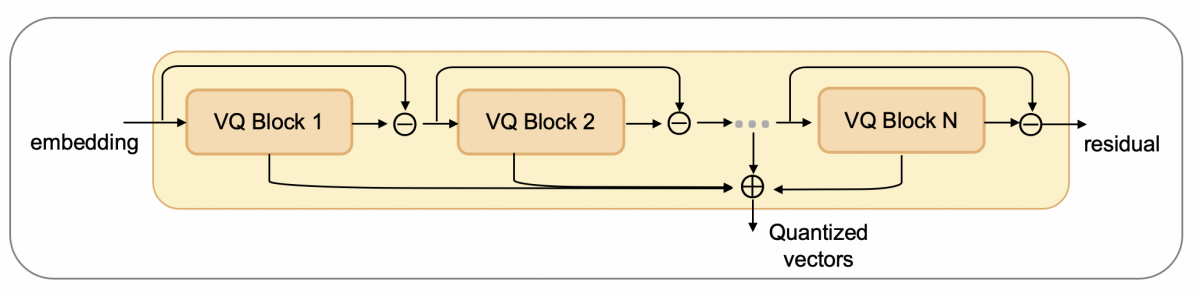
Figure 8. Recursive structure of VQ

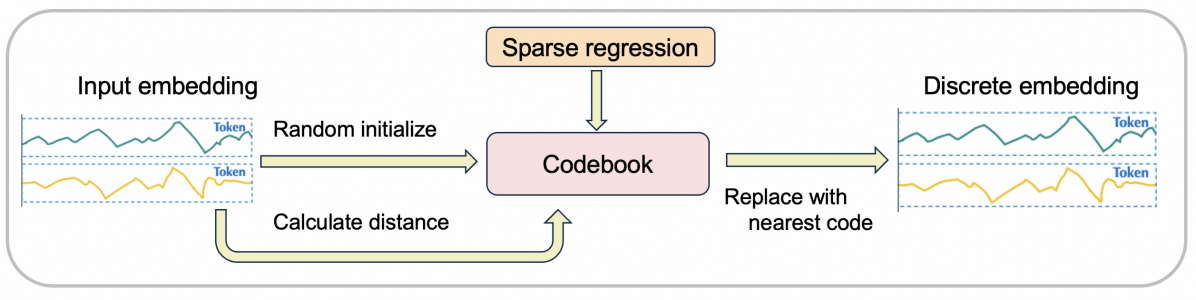
Figure 9. VQ with adaptive codebook

Further exploring the capabilities of VQ, we conducted a series of experiments to evaluate the impact of diverse VQ configurations: (a) $SVQ$: Sparse-VQ; (b) $VQ$: traditional Vector Quantization implemented in the decoder; (c) $VQ_{cosine}$: Vector Quantization using cosine similarity to measure distances; (d) $VQ_{K-means}$: Vector Quantization with a codebook initialized by K-means clustering centroids; (e) $VQ_{recursive}$: employing multiple vector quantizers recursively to quantize the residuals of layer outputs, as shown in Figure 8; and (f) $VQ_{AdaptiveCodebook}$: Vector Quantization with an adaptive codebook learned via sparse regression, detailed in Figure 9. The empirical findings from these experimental studies are detailed in Table 1.

After analyzing the limitations of the standard VQ approach, we introduce Sparse-VQ as the focal point of our research, while also conducting comprehensive evaluations of various VQ design alternatives.

Table 2. Univariate long-term series forecasting results of traditional transformer with Vector Quantization incorporated before the encoder(VQ-pre) and after the decoder(VQ-post). Input length $=512$ and prediction length $=96$. A lower MSE indicates better performance. All experiments are repeated three times.

Methods	PatchTST		VQ-pre		VQ-post
Metric	MSE	MAE	MSE	MAE	MSE	MAE
ettm2	0.065	0.187	0.067	0.191	0.068	0.196
electricity	0.209	0.321	0.226	0.331	0.237	0.341
traffic	0.134	0.223	0.125	0.203	0.135	0.219
weather	0.0013	0.0265	0.0009	0.0217	0.0009	0.0223
wind	2.563	1.261	2.875	1.295	3.017	1.322
nordpool	0.856	0.714	0.912	0.712	0.950	0.719
caiso	0.162	0.279	0.161	0.277	0.169	0.284

Algorithm 1 Sparse-VQ

1:$y=Encoder(x)$, the output of the encoder;

2:The quantized $\hat{y}$;

3:Randomly initialize a leanrnable codebook $Z\in R^{D\times C}$;

4:Calculate Euclidean Distance between the embedding $y$ and $Z$;

5:Replace the embedding $y$ with its nearest neighbor in the codebook to reconstruct the discrete $\hat{y}$;

6:$\hat{y}=SparseRegression(\hat{y})$;

4.3. FFN-free Transformer

Table 3. Univariate forecasting results by PatchTST without ReverseNorm.

woReverseNorm		traffic				weather				ETTm2
PredLen		96	192	336	720	96	192	336	720	96	192	336	720
PatchTST_wFFN	MSE	0.393	0.403	0.414	0.404	0.0450	0.0418	0.0347	0.0371	0.435	0.417	0.487	0.439
	MAE	0.454	0.460	0.468	0.462	0.1643	0.1622	0.1469	0.1517	0.455	0.433	0.464	0.425
PatchTST_woFFN	MSE	0.425	0.415	0.416	0.416	0.0442	0.0463	0.0364	0.0376	0.569	0.619	0.602	0.591
	MAE	0.479	0.470	0.470	0.467	0.1640	0.1706	0.1505	0.1540	0.558	0.603	0.600	0.585

We have opted to integrate a FFN-free architecture into our model. It is inspired by research of the effects of Feed-Forward networks (FFN) in natural language processing (Geva et al., 2021b), which suggests that FFN serves as key-value memories, enabling the preservation of contextual information in datasets with significant scale. In the context of language modeling, key-value memory is essentially to memorize co-occurrence of different tokens (e.g. skip grams (Geva et al., 2020)), a special form of high order statistics from training data, implying that the main role of the FFN module is to compute and store the data statistics for prediction. Following this speculation of the FNN module, we argue if it is appropriate to use the FFN module for non-stationary distribution where statistics of different orders vary significantly over time.

Table 4. Model parameter comparison for PatchTST and PatchTST with FFN-free structure, both the input length $=512$, univariate prediction length $O\in\{96,192,336,720\}$. The amount of parameters is expressed in millions (M).

$Param(M)$	96	192	336	720
PatchTST	0.604	0.801	1.096	1.883
$FFN_{free}$	0.406	0.603	0.898	1.685
Reduction	$\downarrow 32.78\%$	$\downarrow 24.72\%$	$\downarrow 18.07\%$	$\downarrow 10.52\%$

Thus, we first investigate if the FFN module aids in retaining statistical measures (e.g. mean and variance) in the realm of time series forecasting. To this end, we conduct experiments of time series forecasting without using RevIN (Kim et al., 2022), which is used to normalize time series data by local mean and variance. According to Table 3, we observe that, in the case of not using RevIN for data normalization, introducing FFN does significantly improve prediction accuracy, partially validating the hypothesis that the FFN module is used to capture the data statistics. Since both RevIN and FFN capture data statistics, it is thus redundant to include two different modules for the same role. In addition, since RevIN captures local mean and variance, it is more suitable for non-stationary distribution. This is in contrast to the FNN module, where static statistics are stored. In fact, our ablation study in Table  LABEL:tab:ablation_modules shows that when using RevIN for data normalization, removing FFN from transformer can enhance prediction performance, partially validating the hypothesis that RevIN and FFN play similar, or sometimes even conflicting (i.e. stationary vs. drifting distributions) roles in time series forecasting.

Moreover, within the time series domain, which typically features data of relatively low-rank dimensions (e.g., the seasonality of time series can be considered as a low-rank structure), the risk of overfitting is exacerbated. Our FFN-free architecture addresses this issue by effectively reducing the number of parameters by an average of 21.52%, as detailed in Table 4. The reduction of model complexity further justifies the removal of FFN module by improving both computational efficiency and model generalization.

4.4. Optimization

Prediction Loss. We utilize the MAE loss to measure the discrepancy between the prediction and the ground truth, which can be written as:

(1) $$\mathbb{L}_{pred}=\frac{1}{M}\sum_{i=1}^{M}{\frac{1}{T}\sum_{j=1}^{T}\left|\hat{x}_{L+j}^{(i)}-x_{L+j}^{(i)}\right|},$$

where $M$ is the number of channels of the time series and $T$ is the prediction length.

Commitment Loss. We also add the commitment loss to promote the proximity of the input to the selected codebook vector and minimize variations among codebook embeddings, thereby ensuring that the input does not frequently switch between different codebook embeddings. The commitment loss is formulated as follows:

(2) $$\mathbb{L}_{ct}={\|sg[x]-vq(x)\|}_{2}^{2}+{\|x-sg[vq(x)]\|}_{2}^{2},$$

where $sg$ represents the stop-gradient operator, which has partial derivatives equal to zero and remains constant during forward computation; $vq(x)$ denotes the output of Vector Quantization.

Optimization. Formally, our total loss function is defined as:

(3) $$\mathbb{L}=\mathbb{L}_{pred}+\lambda_{1}\mathbb{L}_{ct},$$

where $\lambda_{1}>0$ is the hyperparameter.

5. Experiments

5.1. Dataset and implementation details

We have rigorously assessed our proposed Sparse-VQ model across ten well-established real-world benchmarks, encompassing ETT (m1, m2, h1, h2), Electricity, Traffic, Weather, Wind, Nordpool, and Caiso. For brevity, only the results for the ETTm2 dataset are presented. Comprehensive details about the datasets and the nuances of our implementation are available in Appendix B.

Table 5. Univariate long-term forecasting task. All the results are averaged from 4 different prediction lengths $\in\{96,192,336,720\}$. A lower MAE indicates better performance. All experiments are repeated 3 times. Appendix B.3 shows the full results.

Methods	SVQ		PatchTST		OFA		Dlinear		FEDformer		Autoformer		Informer		LogTrans		Reformer
Metric	MSE	MAE	MSE	MAE	MSE	MAE	MSE	MAE	MSE	MAE	MSE	MAE	MSE	MAE	MSE	MAE	MSE	MAE
ETTm2	0.111	0.248	0.113	0.252	0.119	0.272	0.112	0.248	0.118	0.2595	0.130	0.271	0.175	0.320	0.130	0.277	0.134	0.288
Electricity	0.245	0.348	0.267	0.367	0.292	0.380	0.252	0.355	0.326	0.418	0.414	0.479	0.624	0.598	0.410	0.473	0.352	0.435
Traffic	0.117	0.190	0.136	0.228	0.156	0.261	0.128	0.204	0.177	0.27	0.261	0.365	0.309	0.388	0.355	0.404	0.375	0.434
Weather	0.0013	0.0253	0.0016	0.0294	0.0017	0.0311	0.0061	0.0645	0.007	0.0615	0.0083	0.07	0.0033	0.044	0.0058	0.057	0.0077	0.069
Wind	2.794	1.351	3.084	1.414	3.456	1.530	3.207	1.425	3.808	1.638	3.821	1.648	3.960	1.506	4.654	1.622	3.851	1.489
Nordpool	0.798	0.684	0.890	0.740	0.896	0.743	0.887	0.743	0.876	0.754	0.999	0.8	0.849	0.728	0.882	0.729	0.873	0.739
Caiso	0.233	0.324	0.241	0.340	0.264	0.3495	0.243	0.331	0.269	0.376	0.323	0.414	0.299	0.4	0.288	0.393	0.271	0.380

Table 6. Multivariate long-term series forecasting results on four datasets with same input length $=512$ and various prediction lengths $\in\{96,192,336,720\}$ . A lower MAE indicates better performance. All experiments are repeated 3 times. Full results of four ETT datasets are in Appendix B.3 .

Methods		SVQ		PatchTST		OFA		Dlinear		FEDformer		Autoformer		Informer		LogTrans		Reformer
Metric		MSE	MAE	MSE	MAE	MSE	MAE	MSE	MAE	MSE	MAE	MSE	MAE	MSE	MAE	MSE	MAE	MSE	MAE
ETTm2	96	0.158	0.242	0.166	0.256	0.173	0.262	0.167	0.26	0.203	0.287	0.255	0.339	0.705	0.69	0.768	0.642	0.365	0.453
	192	0.215	0.282	0.223	0.296	0.229	0.301	0.224	0.303	0.269	0.328	0.281	0.34	0.924	0.692	0.989	0.757	0.533	0.563
	336	0.268	0.317	0.274	0.329	0.286	0.341	0.281	0.342	0.325	0.366	0.339	0.372	1.364	0.877	1.334	0.872	1.363	0.887
	720	0.349	0.371	0.362	0.385	0.378	0.401	0.397	0.421	0.421	0.415	0.422	0.419	0.877	1.074	3.048	1.328	3.379	1.338
	Avg	0.248	0.303	0.256	0.317	0.267	0.326	0.267	0.332	0.305	0.349	0.324	0.368	0.968	0.833	1.535	0.900	1.41	0.810
Electricity	96	0.127	0.216	0.129	0.222	0.139	0.238	0.14	0.237	0.183	0.297	0.201	0.317	0.304	0.405	0.258	0.357	0.274	0.368
	192	0.144	0.233	0.147	0.24	0.153	0.251	0.153	0.249	0.195	0.308	0.222	0.334	0.313	0.413	0.266	0.368	0.296	0.386
	336	0.161	0.251	0.163	0.259	0.169	0.266	0.169	0.267	0.212	0.313	0.231	0.338	0.29	0.381	0.28	0.38	0.3	0.394
	720	0.197	0.284	0.197	0.29	0.206	0.297	0.203	0.301	0.231	0.343	0.254	0.361	0.262	0.344	0.283	0.376	0.373	0.439
	Avg	0.157	0.246	0.159	0.253	0.167	0.263	0.166	0.264	0.205	0.315	0.227	0.338	0.292	0.386	0.272	0.370	0.311	0.397
Traffic	96	0.377	0.241	0.36	0.249	0.388	0.282	0.41	0.282	0.562	0.349	0.613	0.388	0.824	0.514	0.684	0.384	0.719	0.391
	192	0.390	0.247	0.379	0.256	0.407	0.290	0.423	0.287	0.562	0.346	0.616	0.382	1.106	0.672	0.685	0.39	0.696	0.379
	336	0.399	0.252	0.392	0.264	0.412	0.294	0.436	0.296	0.57	0.323	0.622	0.337	1.084	0.627	0.733	0.408	0.777	0.42
	720	0.438	0.275	0.432	0.286	0.450	0.312	0.466	0.315	0.596	0.368	0.66	0.408	1.536	0.845	0.717	0.396	0.864	0.472
	Avg	0.401	0.254	0.391	0.264	0.414	0.295	0.434	0.295	0.573	0.347	0.628	0.379	1.138	0.665	0.705	0.395	0.764	0.416
Weather	96	0.145	0.183	0.149	0.198	0.162	0.212	0.176	0.237	0.217	0.296	0.266	0.336	0.406	0.444	0.458	0.49	0.3	0.384
	192	0.188	0.228	0.194	0.241	0.204	0.248	0.22	0.282	0.276	0.336	0.307	0.367	0.525	0.527	0.658	0.589	0.598	0.544
	336	0.238	0.269	0.245	0.282	0.254	0.286	0.265	0.319	0.339	0.38	0.359	0.395	0.531	0.539	0.797	0.652	0.578	0.523
	720	0.306	0.321	0.314	0.334	0.326	0.337	0.323	0.362	0.403	0.428	0.578	0.578	0.419	0.428	0.869	0.675	1.059	0.741
	Avg	0.219	0.250	0.226	0.264	0.237	0.271	0.246	0.3	0.309	0.36	0.378	0.419	0.470	0.485	0.696	0.602	0.634	0.548
Wind	96	0.886	0.622	0.894	0.639	0.942	0.657	0.902	0.649	1.438	0.892	1.475	0.900	1.422	0.803	1.497	0.849	1.097	0.705
	192	1.133	0.748	1.166	0.782	1.168	0.774	1.124	0.766	1.572	0.945	1.720	0.973	1.810	0.950	1.574	0.911	1.279	0.783
	336	1.275	0.841	1.374	0.875	1.387	0.872	1.329	0.862	1.815	1.031	1.667	0.968	1.714	0.926	1.551	0.918	1.471	0.897
	720	1.418	0.910	1.545	0.955	1.587	0.955	1.495	0.935	1.788	1.021	1.738	1.000	1.877	0.990	1.602	0.952	1.502	0.944
	Avg	1.178	0.780	1.245	0.813	1.271	0.815	1.213	0.803	1.653	0.972	1.65	0.960	1.706	0.917	1.556	0.908	1.337	0.832
Nordpool	96	0.543	0.540	0.560	0.558	0.563	0.556	0.613	0.593	0.552	0.579	0.815	0.702	1.029	0.788	0.858	0.691	0.645	0.618
	192	0.608	0.579	0.632	0.594	0.613	0.590	0.674	0.636	0.646	0.634	0.795	0.697	1.030	0.804	0.918	0.715	0.728	0.659
	336	0.593	0.578	0.596	0.594	0.595	0.587	0.653	0.628	0.599	0.593	0.829	0.713	1.198	0.860	0.953	0.744	0.782	0.675
	720	0.585	0.580	0.586	0.590	0.580	0.587	0.642	0.627	0.634	0.624	0.736	0.672	1.246	0.865	0.997	0.759	0.836	0.694
	Avg	0.582	0.569	0.594	0.584	0.588	0.58	0.646	0.621	0.608	0.608	0.794	0.696	1.126	0.829	0.932	0.727	0.748	0.662
Caiso	96	0.204	0.286	0.237	0.307	0.210	0.297	0.221	0.302	0.265	0.365	0.327	0.406	0.320	0.394	0.261	0.355	0.242	0.343
	192	0.279	0.341	0.323	0.364	0.276	0.349	0.279	0.350	0.325	0.413	0.462	0.499	0.415	0.457	0.295	0.378	0.285	0.372
	336	0.331	0.376	0.370	0.402	0.330	0.389	0.328	0.388	0.345	0.421	0.584	0.552	0.473	0.492	0.368	0.458	0.343	0.455
	720	0.430	0.428	0.456	0.458	0.466	0.456	0.450	0.459	0.416	0.471	0.505	0.517	0.536	0.533	0.506	0.503	0.498	0.489
	Avg	0.311	0.357	0.347	0.383	0.321	0.373	0.320	0.375	0.338	0.418	0.470	0.494	0.436	0.469	0.358	0.424	0.342	0.415

5.2. Long-term Forecasting

For better comparison, we follow the experiment settings of PatchTST (Nie et al., 2022) where the input length is fixed to 512, and the prediction lengths for both training and evaluation are fixed to be 96, 192, 336, and 720, respectively.

Univariate Results

For univariate time series forecasting, Sparse-VQ achieves the best performance on all seven benchmark datasets at all horizons as shown in Table 5. Compared to PatchTST, Sparse-VQ yields an overall 7.84% relative MAE reduction. On some datasets, such as traffic and weather, the improvement is more than 15%. The experimental results in Table 5 verifies that Sparse-VQ is very effective in long-term forecasting.

Multivariate Results

The results for multivariate time series forecasting are summarized in Table 6. Compared with PatchTST, the proposed Sparse-VQ yields an overall 4.17% relative MAE reduction. Overall, the improvement made by Sparse-VQ is consistent with varying horizons, implying its strength in long term forecasting.

Table 7. Short-term forecasting task on M4. The prediction lengths are $\in\{6,48\}$ and results are weighted averaged from several datasets under different sample intervals. A lower score indicates better performance. All experiments are repeated 3 times.Full results are in Appendix B.4

Methods		SVQ	OFA	PatchTST	N-HiTS	N-BEATS	ETSformer	LighTS	Dlinear	FEDformer	Autoformer	Informer	Reformer
Average	SMAPE	11.938	11.991	12.059	11.927	11.851	14.718	13.525	13.639	12.840	12.909	14.086	18.200
	MASE	1.593	1.600	1.623	1.613	1.599	2.408	2.111	2.095	1.701	1.771	2.718	4.223
	OWA	0.857	0.861	0.869	0.861	0.855	1.172	1.051	1.051	0.918	0.939	1.230	1.775

Table 8. Few-shot learning results on 5% data. All the results are averaged from 4 different prediction lengths $\in\{96,192,336,720\}$ .A lower MSE indicates better performance, and the best results are highlighted in bold. Full results are in Appendix B.5

Methods	SVQ		PatchTST		OFA		Dlinear		FEDformer		Autoformer		Informer		LogTrans		Reformer
Metric	MSE	MAE	MSE	MAE	MSE	MAE	MSE	MAE	MSE	MAE	MSE	MAE	MSE	MAE	MSE	MAE	MSE	MAE
ETTm1	0.405	0.412	0.526	0.476	0.472	0.45	0.400	0.417	0.73	0.592	0.796	0.62	1.163	0.791	1.597	0.979	1.264	0.826
Electricity	0.185	0.281	0.181	0.277	0.178	0.273	0.176	0.275	0.266	0.353	0.346	0.404	1.281	0.929	0.934	0.746	1.289	0.904
Traffic	0.426	0.288	0.418	0.296	0.434	0.305	0.45	0.317	0.676	0.423	0.833	0.502	1.591	0.832	1.309	0.685	1.618	0.851
Weather	0.258	0.283	0.269	0.303	0.263	0.301	0.263	0.308	0.309	0.353	0.31	0.353	0.584	0.527	0.457	0.458	0.447	0.453
Wind	1.321	0.830	1.469	0.892	1.489	0.898	1.396	0.869	1.741	1.005	1.893	1.038	4.183	1.622	3.847	1.558	2.594	1.320
Nordpool	0.654	0.608	0.711	0.642	0.752	0.656	0.71	0.646	0.954	0.766	0.994	0.784	3.158	1.430	2.171	1.188	1.99	1.142
Caiso	0.319	0.366	0.386	0.426	0.382	0.431	0.382	0.426	0.653	0.599	0.729	0.633	1.785	0.966	1.664	0.922	1.433	0.862

5.3. Short-term Forecasting

To thoroughly assess different algorithms in forecasting, we extend our experiments to the M4 dataset (Makridakis et al., 2018) for short-term forecasting, which consists of univariate marketing data across yearly, quarterly, and monthly frequencies with a comparatively brief forecast horizon. Unlike the long-term datasets that feature a single continuous series from which samples are drawn using sliding windows, the M4 dataset is composed of 100,000 unique series collected at varying intervals.

Table 7 highlights Sparse-VQ’s superior performance against both advanced transformer-based and MLP-based models. Notably, when pitted against the similar transformer-based PatchTST method, Sparse-VQ achieves improvements of 1%, 1.8%, and 1.4% in SMAPE, MASE, and OWA, respectively, and it exhibits performance on par with the N-BEATS method.

5.4. Few-shot Forecasting

Few-shot learning poses a unique challenge in forecasting, where models must forge robust representations from scant data. To probe Sparse-VQ’s capability for time series analysis under this stringent condition, we devised targeted experiments. Deviating from the usual division of data into training, validation, and test segments, our few-shot approach operates with a mere sliver (e.g., 5%, 10%) of the training data. Table 8 encapsulates Sparse-VQ’s impressive average outcomes using only 5% of the data, outstripping recent cutting-edge methods such as OFA and PatchTST.Remarkably, in comparison to the transformer-based PatchTST method, Sparse-VQ records average enhancements of 9.5% in mse and 7.2% in mae across all benchmarks. A full exposition of our extensive findings over ten datasets is available in Appendix B.5.

5.5. Ablations

5.5.1. Validity analysis of several modules

The ablation study in Table 9 provides important insights into how the Sparse-VQ and FFN-free structure affect the performance of our framework. We compare our results with PatchTST, which is considered the state-of-the-art benchmark for transformer-based models. By analyzing the results with and without Sparse-VQ / FFN-free structure, we can observe that both of these factors play significant roles in improving the forecasting performance.

When using the FFN-free structure, we observe a 4.36% decrease in MAE compared to the original model, suggesting that the FFN-free structure contributes to enhancing the model’s forecasting performance. Furthermore, building upon the the FFN-free structure, integration of Sparse-VQ can achieve a 5.04% reduction in MAE, whereas incorporating VQ yields a mere 1.21% decrease by comparison, highlighting the importance of the sparse structure.

To explore how Sparse-VQ and FFN-free structures enhance the predictive accuracy of the model, we generate and plot the distribution of the model embeddings. Figure 4 shows that both the two modules effectively concentrate the distribution of embeddings, thereby improving the performance of the model. Also, we employed t-SNE to reduce the dimensions of the codebooks from VQ and Sparse-VQ, facilitating their visualization as depicted in the Figure 5. The results clearly demonstrate that Sparse-VQ encompasses a wider representational range and presents a distribution that is more uniform and continuous than VQ.

Table 9. Ablation study of FFN-free and Sparse-VQ in PatchTST. 4 cases are included: (a) both FFN-free and Sparse-VQ are included in model (SVQ+FFN-f); (b) only Vector Quantization (VQ+FFN-f); (c) only FFN-free(FFN-f);(d) neither of them is included (Original patchTST model). The best results are in bold. A lower MSE indicates better performance. Appendix B.6 shows the full results.

Methods	SVQ+FFN-f		VQ+FFN-f		FFN-f		Original
Metric	MSE	MAE	MSE	MAE	MSE	MAE	MSE	MAE
ETTm2	0.111	0.248	0.111	0.249	0.112	0.250	0.113	0.252
Electricity	0.245	0.348	0.253	0.353	0.256	0.355	0.267	0.365
Weather	0.0013	0.0253	0.0015	0.0280	0.0015	0.0287	0.0016	0.0294
Traffic	0.117	0.190	0.120	0.199	0.122	0.202	0.136	0.228

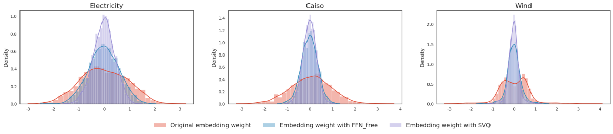
Figure 4. Distribution of embedding weight. Sparse-VQ framework encourages denser weights

5.5.2. Sparse-VQ

The codebook size dictates the embedding capacity for diverse time series patterns and consequently affects sparse-VQ’s performance. As evidenced in Table 12, enlarging the codebook size generally enhances model accuracy. However, excessively large codebooks can hinder convergence and ultimately reduce accuracy.

Moreover, we would like to highlight the generality of our Sparse-VQ, which can serve as a plug-in to enhance the performance of other models. To demonstrate the general applicability of Sparse-VQ, we employ it in FEDformer (Zhou et al., 2022a), Autoformer (Wu et al., 2021). The results are summarized in Table 10. Integrating the Vector Quantization structure yields a modest boost, enhancing the FEDformer by 2.01% and the Autoformer by 3.63% in MSE. Notably, these improvements are consistent across models with varying predictive capabilities, suggesting that this could be a beneficial addition following the development of base models.

Table 10. Results for boosting effect of sparse-VQ. All the results are averaged from 4 different prediction lengths $\in\{96,192,336,720\}$. We use FEDformer and Autoformer as backbones and leverage them with the Sparse-VQ. A lower MSE indicates better performance. All experiments are repeated 3 times. Appendix B.6 shows the full results.

Methods	FEDformer		FEDformer+SVQ		Autoformer		Autoformer+SVQ
Metric	MSE	MAE	MSE	MAE	MSE	MAE	MSE	MAE
ETTm2	0.305	0.349	0.303	0.351	0.324	0.368	0.306	0.350
Electricity	0.214	0.327	0.209	0.323	0.227	0.338	0.232	0.333
Traffic	0.610	0.376	0.606	0.373	0.628	0.379	0.625	0.389
Weather	0.309	0.360	0.296	0.348	0.338	0.382	0.308	0.356

5.5.3. Robustness analysis

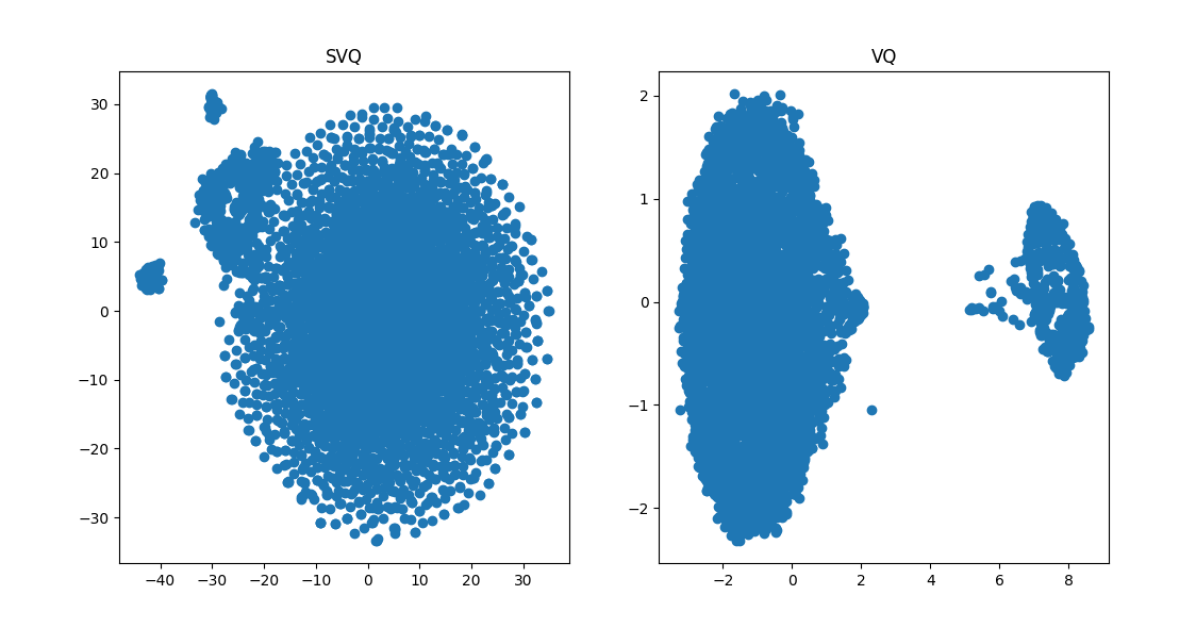
Figure 5. Distribution of codebook. Sparse-VQ encourage a sparser codebook with a wider range of perception.

Table 11. Robustness analysis of univariate results conducted on four typical datasets. The degree of noise injected into the time series data is determined by $\eta$. All the results are averaged from 4 different prediction lengths $\in\{96,192,336,720\}$.All experiments are repeated 3 times. Appendix B.8 shows the full results.

VQ	Original		$\eta=1\%$		$\eta=5\%$		$\eta=10\%$
Metric	MSE	MAE	MSE	MAE	MSE	MAE	MSE	MAE
ETTm2	0.111	0.248	0.112	0.250	0.114	0.253	0.114	0.255
Electricity	0.253	0.353	0.254	0.355	0.258	0.356	0.265	0.368
Traffic	0.120	0.199	0.121	0.201	0.125	0.212	0.138	0.239
Weather	0.0015	0.028	0.0015	0.028	0.0015	0.0282	0.0015	0.029

Table 12. SVQ with different size of codebook. A lower MSE indicates better performance. All experiments are repeated three times on average.

Codebook Size	10		750		10000
Metric	MSE	MAE	MSE	MAE	MSE	MAE
Caiso	0.500	0.471	0.451	0.454	0.480	463
Weather	0.315	0.341	0.306	0.322	0.322	0.349
ETTm2	0.372	0.393	0.356	0.376	0.367	0.389

To evaluate the robustness of our model, we follow a commonly used practice by introducing noise into the data and then training the modified dataset, which is based on the approach described in the MICN (Wang et al., 2023). The experimental results are presented in Table 11. The results show a slight increase in both metrics of Sparse-VQ as the amount of injected noise increases, while the prediction effect of other models have large fluctuations. Owing to space constraints, we present comprehensive results in Appendix B.8. For instance, under 10% noise, Sparse-VQ exhibits a relative MAE increase of 6.3%, compared to 8.9% for PatchTST and 12.7% for FEDformer, as detailed in appendix Tables  23 and  24. Our findings reveal that our model, bolstered by its unique quantization approach, surpasses baseline counterparts in noise robustness.

6. Conclusion

In summary, our research addresses the unique challenges of time series analysis—distribution shifts and high noise levels—by proposing the Sparse Vector Quantized FFN-Free Transformer (Sparse-VQ). This innovative model reimagines the transformer architecture sans the conventional Feed-Forward layer, utilizing Sparse-VQ and Reverse Instance Normalization (RevIN) for noise reduction and statistical capture. This leads to a more efficient model with fewer parameters, which not only reduces overfitting but also enhances computational performance. Our Sparse-VQ model has demonstrated superior accuracy, outperforming established models with significant reductions in MAE on average (7.84% for univariate and 4.17% for multivariate forecasting), as validated on ten benchmark datasets, including the novel CAISO dataset. Furthermore, Sparse-VQ’s design allows for easy integration with existing transformer-based models, improving their efficacy in time series forecasting. We encourage the community to explore beyond the adaptation of traditional transformers for time series analysis by meticulously dissecting transformer components. A more efficient alternative tailored to these applications may well be within closer reach than anticipated.

Appendix A Related Work

A.1. Time-series Forecasting

Temporal variation modeling is a prominent issue in time series analysis and has been extensively investigated with numerous methods been proposed to achieve accurate long-term time series forecasting.

Early studies typically employed traditional statistical methods or machine learning techniques, such as ARIMA (Box and Jenkins, 1968), Holt-Winter (Hyndman and Athanasopoulos, 2018), DeepAR (Salinas et al., 2020) and Prophet (Taylor and Letham, 2018). With the rise of deep learning, researchers have turned their attention to more robust and complex neural networks for time series modeling, including TCN (Bai et al., 2018), LSTM (Hochreiter and Schmidhuber, 1997). Specifically, N-BEATS (Oreshkin et al., 2019) designed an interpretable layer by encouraging the model to learn trend, seasonality explicitly, and residual components, which shows superior performance on the M4 competition dataset; Dlinear (Zeng et al., 2022) employs a simple linear layer, while TimesNet (Wu et al., 2022) extends the analysis of temporal variations into the 2D space enabling to discover the multi-periodicity adaptively and extract the complex temporal variations.

Among these, the Transformer (Vaswani et al., 2017) and its subsequent adaptations have demonstrated significant success in long sequence modelling tasks, including time series forecasting. Informer (Zhou et al., 2021) proposes a ProbSparse self-attention mechanism and distilling operation to address the quadratic complexity of the Transformer, while Reformer (Kitaev et al., 2020) replaces dot-product attention by using locality-sensitive hashing and improves its complexity, resulting in significant performance improvements. Subsequently, Autoformer (Wu et al., 2021) designs an efficient auto-correlation mechanism to discover and aggregate information at the series level; FiLM (Zhou et al., 2022b) design a Frequency improved Legendre Memory model applying Legendre polynomial projections to approximate historical information, while FEDformer (Zhou et al., 2022a) proposes an attention mechanism with low-rank approximation in frequency and a mixture of experts decomposition to control the distribution shifting. Additionally, Pyraformer (Liu et al., 2022) designs pyramidal attention to effectively describe short and long temporal dependencies with low time and space complexity and patchTST (Nie et al., 2022) embeds the whole time series of each variate independently into tokens to enlarge local receptive field. GCformer (Zhao et al., 2023) combines a structured global convolutional branch with a local Transformer-based branch to capture the long and short signals at the same time. Recently, FPT (Zhou et al., 2023) leverages pretrained language or CV models for time series analysis firstly and achieves excellent performance in all main time series analysis tasks. Overall, the Transformer architecture is widely regarded as one of the most effective and promising approaches for MTS forecasting (Wen et al., 2022; Shao et al., 2023)).

A.2. Distribution shift

Although various models above make breakthroughs in time-series forecasting, they often encounter challenges when dealing with non-stationary time-series data, where the distribution of the data changes over time. To address this issue, domain adaptation (Tzeng et al., 2017; Ganin et al., 2016; Wang et al., 2018) and domain generalization (Wang et al., 2021; Li et al., 2018; Muandet et al., 2013; Lu et al., 2022)) approaches are commonly employed to mitigate the distribution shift. Domain adaptation algorithms aim to reduce the distribution gap between the source and target domains, while domain generalization algorithms solely rely on the source domain and aim to generalize to the target domain. However, defining a domain becomes challenging in the context of non-stationary time series, as the data distribution shifts over time. Recently, (Du et al., 2021) proposes the use of Adaptive RNNs to address the distribution shift issues in non-stationary time-series data, characterizing the distribution information by dividing the training data into periods and then matches the distributions of these identified periods to generalize the model. RevIN (Kim et al., 2021) utilizes a generally applicable normalization-and-denormalization method with learnable affine transformation to address the distribution shift problem. DIVERSIFY (Lu et al., 2023) trys to learn the out of-distribution (OOD) representation on dynamic distributions of times series and then bridges the gap between these latent distributions.

A.3. Vector Quantization

Vector quantization (VQ) is a widely used compression technique in signal and image processing, which aims to learn a discrete latent representation by clustering multidimensional data into a finite set of representations. VQ-VAE (van den Oord et al., 2017) proposes to combine the VQ strategy with a variational autoencoder. There are two key differences between this approach and VAEs: first, the encoder network produces discrete codes instead of continuous ones to obtain a compressed discrete latent space; second, the prior is learned rather than being static; which make it capable of modelling very long term dependencies. SoundStream (Zeghidour et al., 2022) proposes the residual VQ and employs multiple vector quantizers to iteratively quantize the residuals of the waveform.VQ has also been combined with adversarial learning to synthesize high-resolution images, for example, VQGAN  (Yu et al., 2022a). Subsequently, ViT-VQGAN (Yu et al., 2022b) proposes to reduce the dimensionality of the codebook and l2-normalize the codebook and TE-VQGAN (Shin et al., 2021) incorporate a regularization term into the loss function to enforce orthogonality among the codebook embeddings. Recent works (Lee et al., 2023; Lendasse et al., 2005; Rasul et al., 2022) have applyed Vector Quantization (VQ) to time series domain. Considering veiwing time series as several discrete tokens may be potentially useful, our framework uniquely leverages VQ to enhance the capabilities of transformers in time series forecasting.

Appendix B Supplemental Experiments

B.1. Dataset Details

We extensively evaluate the performance of the proposed Sparse-VQ on eight widely used real-world benchmarks, the details of the datasets used in this article are as follows: 1) ETT dataset (Zhou et al., 2021) is collected from two separate counties in two versions of the sampling resolution (15 minutes & 1 h). The ETT dataset contains several time series of electric loads and time series of oil temperature. 2) A dataset called Electricity contains data on the electricity consumption of more than 300 customers and each column corresponds to the same client. 3) Traffic dataset records the occupation rate of highway systems in California, USA. 4) The Weather dataset contains 21 meteorological indicators in Germany for an entire year. 5) NorPool includes eight years of hourly energy production volume series in multiple European countries. 6)Wind (Li et al., 2022) contains wind power records from 2020-2021 at 15-minute intervals.

Moreover, we have additionally gathered and processed a novel dataset named CAISO , which contains eight years(2016-2023) of hourly actual electricity load series in different zones of California. Table 13 summarizes all the features of the eight benchmark datasets. We also visualize the time series for univariate prediction in the Figure 6 to show different property of these datasets.

During the experiment, they are divided into training sets, validation sets, and test sets in a 6:2:2 ratio during modeling for ETT and Wind, and 7:1:2 for Weather, Traffic, Electricity, Nordpool and Caiso.

Table 13. Details of ten benchmark datasets.

Dataset	Length	Dimension	Frequency
ETTm1/m2	69680$\approx$2 years	7	15 min
ETTh1/h2	17420$\approx$2 years	7	1h
Electricity	26304$\approx$3 years	321	1h
Traffic	17544$\approx$2 years	862	1h
Weather	52696$\approx$1 years	21	10 min
Wind	48673$\approx$1 years	7	15min
Nordpool	70128$\approx$8 years	18	1h
Caiso	74472$\approx$8 years	10	1h

B.2. Implementation Details

We use ADAM (Kingma and Ba, 2017) optimizer with a learning rate of $1e^{-4}$ to $1e^{-3}$. We save models with the lowest loss in validation sets for the final test. Measurements are made using mean square error (MSE) and mean absolute error (MAE). All experiments are repeated 3 times and the mean of the metrics is reported as the final result. Multivariate forecasting results are runed on NVIDIA A100 80GB GPU and other results are runed on NVIDIA V100 32GB GPU.

B.3. Long-term Time-series forecasting

Here we verify the consistent performance of our architectural framework on the full ten datasets. To ensure the fairness of the experiments, we follow the classical experiment settings of PatchTST (Nie et al., 2022). Table 14 shows the full univariate long-term series forecasting results on ten datasets and Table 17 shows multivariate long-term series forecasting results on four ETT datasets. Table 18 shows the full results of short-term forecasting.

B.4. Short-term Time-series forecasting

We conduct short-term forecasting (with relatively short forecasting horizon) experiments on the M4 dataset (Makridakis et al., 2018). Table 18 shows the full results on marketing data of various frequencies, which show that the performance of Sparse-VQ is superior to OFA and PatchTST, comparable to N-BEATS.

B.5. Few-shot Time-series forecasting

During the few-shot forecasting experiment, we only used a certain percentage (5% in Table 15, 10% in Table 16) timesteps of training data and the evaluation metrics employed are consistent with those used in conventional multivariate time series forecasting.

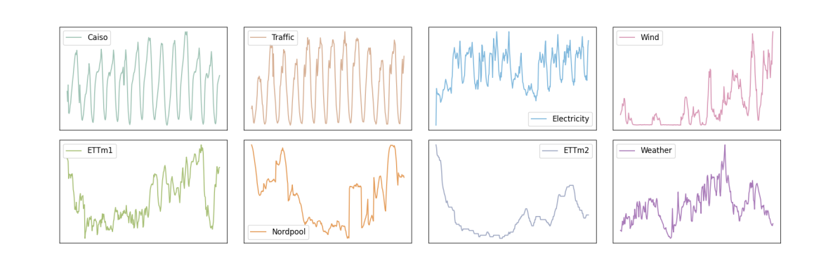
Figure 6. Visualization of the time series of eight datasets for univariate prediction.

Table 14. Univariate long-term series forecasting results on ten datasets with same input length $=512$ and prediction length $\in\{96,192,336,720\}$. A lower MAE indicates better performance. All experiments are repeated 3 times.

Methods		SVQ		PatchTST		OFA		Dlinear		FEDformer		Autoformer		Informer		LogTrans		Reformer
Metric		MSE	MAE	MSE	MAE	MSE	MAE	MSE	MAE	MSE	MAE	MSE	MAE	MSE	MAE	MSE	MAE	MSE	MAE
ETTm1	96	0.025	0.121	0.026	0.123	0.026	0.124	0.028	0.123	0.033	0.140	0.056	0.183	0.109	0.277	0.049	0.171	0.296	0.355
	192	0.039	0.150	0.040	0.151	0.040	0.153	0.045	0.156	0.058	0.186	0.081	0.216	0.151	0.31	0.157	0.317	0.429	0.474
	336	0.050	0.172	0.053	0.174	0.054	0.179	0.061	0.182	0.084	0.231	0.076	0.218	0.427	0.591	0.289	0.459	0.585	0.583
	720	0.068	0.200	0.073	0.206	0.071	0.204	0.080	0.210	0.102	0.25	0.11	0.267	0.438	0.586	0.43	0.579	0.782	0.73
	Avg	0.046	0.161	0.048	0.164	0.048	0.165	0.054	0.168	0.069	0.202	0.081	0.221	0.281	0.441	0.231	0.382	0.523	0.536
ETTm2	96	0.063	0.183	0.065	0.187	0.066	0.191	0.063	0.183	0.063	0.189	0.065	0.189	0.088	0.225	0.075	0.208	0.076	0.214
	192	0.090	0.225	0.093	0.230	0.262	0.098	0.092	0.227	0.102	0.245	0.118	0.256	0.132	0.283	0.129	0.275	0.132	0.29
	336	0.118	0.262	0.122	0.267	0.305	0.134	0.119	0.261	0.13	0.279	0.154	0.305	0.18	0.336	0.154	0.302	0.16	0.312
	720	0.172	0.322	0.173	0.324	0.389	0.176	0.175	0.320	0.178	0.325	0.182	0.335	0.3	0.435	0.16	0.321	0.168	0.335
	Avg	0.111	0.248	0.113	0.252	0.256	0.150	0.112	0.248	0.118	0.260	0.130	0.271	0.175	0.320	0.130	0.277	0.134	0.288
ETTh1	96	0.056	0.184	0.059	0.189	0.061	0.192	0.056	0.180	0.079	0.215	0.071	0.206	0.193	0.377	0.283	0.468	0.532	0.569
	192	0.072	0.210	0.074	0.215	0.077	0.219	0.071	0.204	0.104	0.245	0.114	0.262	0.217	0.395	0.234	0.409	0.568	0.575
	336	0.079	0.224	0.076	0.220	0.075	0.218	0.098	0.244	0.119	0.27	0.107	0.258	0.202	0.381	0.386	0.546	0.635	0.589
	720	0.084	0.231	0.087	0.236	0.090	0.240	0.189	0.359	0.142	0.299	0.126	0.283	0.183	0.355	0.475	0.628	0.762	0.666
	Avg	0.073	0.212	0.074	0.215	0.076	0.217	0.104	0.247	0.111	0.257	0.105	0.252	0.199	0.377	0.345	0.513	0.624	0.600
ETTh2	96	0.133	0.283	0.131	0.284	0.132	0.284	0.131	0.279	0.128	0.271	0.153	0.306	0.213	0.373	0.217	0.379	1.411	0.838
	192	0.174	0.331	0.171	0.329	0.180	0.334	0.176	0.329	0.185	0.330	0.204	0.351	0.227	0.387	0.281	0.429	5.658	1.671
	336	0.181	0.343	0.171	0.336	0.179	0.338	0.209	0.367	0.231	0.378	0.246	0.389	0.242	0.401	0.293	0.437	4.777	1.582
	720	0.215	0.372	0.223	0.380	0.226	0.382	0.276	0.426	0.278	0.42	0.268	0.409	0.291	0.439	0.218	0.387	2.042	1.039
	Avg	0.176	0.332	0.174	0.332	0.179	0.335	0.198	0.350	0.206	0.350	0.218	0.364	0.243	0.4	0.252	0.408	3.472	1.283
ETTm2	96	0.063	0.183	0.065	0.187	0.066	0.191	0.063	0.183	0.063	0.189	0.065	0.189	0.088	0.225	0.075	0.208	0.076	0.214
	192	0.090	0.225	0.093	0.230	0.098	0.262	0.092	0.227	0.102	0.245	0.118	0.256	0.132	0.283	0.129	0.275	0.132	0.29
	336	0.118	0.262	0.122	0.267	0.134	0.305	0.119	0.261	0.13	0.279	0.154	0.305	0.18	0.336	0.154	0.302	0.16	0.312
	720	0.172	0.320	0.173	0.324	0.176	0.328	0.175	0.320	0.178	0.325	0.182	0.335	0.3	0.435	0.16	0.321	0.168	0.335
	Avg	0.111	0.248	0.113	0.252	0.119	0.272	0.112	0.248	0.118	0.2595	0.130	0.271	0.175	0.320	0.130	0.277	0.134	0.288
Electricity	96	0.194	0.304	0.209	0.321	0.212	0.321	0.202	0.314	0.253	0.37	0.341	0.438	0.484	0.538	0.288	0.393	0.274	0.379
	192	0.226	0.325	0.246	0.344	0.266	0.358	0.233	0.336	0.282	0.386	0.345	0.428	0.557	0.558	0.432	0.483	0.304	0.402
	336	0.263	0.358	0.280	0.379	0.306	0.385	0.270	0.364	0.346	0.431	0.406	0.47	0.636	0.613	0.43	0.483	0.37	0.448
	720	0.298	0.404	0.332	0.424	0.383	0.455	0.303	0.406	0.422	0.484	0.565	0.581	0.819	0.682	0.491	0.531	0.46	0.511
	Avg	0.245	0.348	0.267	0.367	0.292	0.380	0.252	0.355	0.326	0.418	0.414	0.479	0.624	0.598	0.410	0.473	0.352	0.435
Traffic	96	0.115	0.183	0.134	0.223	0.145	0.252	0.122	0.194	0.17	0.263	0.246	0.346	0.257	0.353	0.226	0.317	0.313	0.383
	192	0.112	0.182	0.130	0.221	0.148	0.255	0.125	0.199	0.173	0.265	0.266	0.37	0.299	0.376	0.314	0.408	0.386	0.453
	336	0.113	0.190	0.133	0.227	0.156	0.261	0.124	0.202	0.178	0.266	0.263	0.371	0.312	0.387	0.387	0.453	0.423	0.468
	720	0.126	0.204	0.146	0.241	0.173	0.276	0.139	0.222	0.187	0.286	0.269	0.372	0.366	0.436	0.491	0.437	0.378	0.433
	Avg	0.117	0.190	0.136	0.228	0.156	0.261	0.128	0.204	0.177	0.27	0.261	0.365	0.309	0.388	0.355	0.404	0.375	0.434
Weather	96	0.0009	0.0210	0.0013	0.0265	0.0013	0.028	0.0050	0.056	0.0035	0.046	0.011	0.081	0.0038	0.044	0.0046	0.052	0.012	0.087
	192	0.0011	0.0239	0.0014	0.0281	0.0014	0.0295	0.0061	0.065	0.0054	0.059	0.0075	0.067	0.0023	0.04	0.0056	0.06	0.0098	0.079
	336	0.0013	0.0258	0.0015	0.0289	0.0017	0.031	0.0064	0.067	0.0041	0.05	0.0063	0.062	0.0041	0.049	0.006	0.054	0.005	0.059
	720	0.0018	0.0305	0.0021	0.0341	0.0022	0.036	0.0068	0.070	0.015	0.091	0.0085	0.07	0.0031	0.042	0.0071	0.063	0.0041	0.049
	Avg	0.0013	0.0253	0.0016	0.0294	0.0017	0.0311	0.0061	0.0645	0.007	0.0615	0.0083	0.07	0.0033	0.044	0.0058	0.057	0.0077	0.069
Wind	96	2.370	1.211	2.563	1.261	2.683	1.296	2.539	1.239	3.278	1.490	3.177	1.485	3.468	1.395	3.936	1.468	3.110	1.332
	192	2.742	1.338	3.001	1.391	3.310	1.492	3.102	1.395	3.763	1.620	3.645	1.599	3.973	1.502	4.748	1.639	3.912	1.496
	336	2.850	1.385	3.317	1.489	3.764	1.630	3.468	1.496	4.053	1.702	4.192	1.737	4.221	1.568	5.281	1.743	4.024	1.536
	720	3.213	1.471	3.454	1.515	4.067	1.701	3.718	1.568	4.139	1.741	4.270	1.771	4.176	1.558	4.652	1.639	4.359	1.593
	Avg	2.794	1.351	3.084	1.414	3.456	1.530	3.207	1.425	3.808	1.638	3.821	1.648	3.960	1.506	4.654	1.622	3.851	1.489
Nordpool	96	0.871	0.702	0.856	0.714	0.868	0.716	0.853	0.715	0.849	0.736	0.932	0.767	0.921	0.758	0.895	0.720	0.904	0.722
	192	0.776	0.667	0.930	0.748	0.938	0.757	0.926	0.758	0.914	0.777	1.061	0.831	0.848	0.731	0.868	0.727	0.858	0.713
	336	0.777	0.681	0.900	0.749	0.906	0.753	0.896	0.752	0.863	0.747	0.966	0.785	0.812	0.709	0.855	0.725	0.877	0.754
	720	0.768	0.687	0.872	0.747	0.871	0.746	0.873	0.748	0.878	0.755	1.035	0.817	0.816	0.713	0.909	0.745	0.851	0.767
	Avg	0.798	0.684	0.890	0.740	0.896	0.743	0.887	0.743	0.876	0.754	0.999	0.8	0.849	0.728	0.882	0.729	0.873	0.739
Caiso	96	0.140	0.255	0.162	0.279	0.169	0.285	0.151	0.262	0.191	0.327	0.227	0.353	0.217	0.337	0.206	0.311	0.207	0.340
	192	0.211	0.308	0.212	0.322	0.233	0.328	0.215	0.312	0.247	0.367	0.262	0.370	0.293	0.394	0.254	0.360	0.221	0.344
	336	0.257	0.342	0.263	0.355	0.281	0.361	0.259	0.346	0.266	0.360	0.299	0.399	0.302	0.405	0.310	0.422	0.298	0.396
	720	0.325	0.391	0.325	0.403	0.373	0.424	0.346	0.404	0.372	0.451	0.504	0.535	0.382	0.464	0.380	0.479	0.356	0.441
	Avg	0.233	0.324	0.241	0.340	0.264	0.3495	0.243	0.331	0.269	0.376	0.323	0.414	0.299	0.4	0.288	0.393	0.271	0.380

Table 15. Few-shot learning results of four ETT datasets on 5% data. We use prediction length $O\in\{96,192,336,720\}$.A lower MSE indicates better performance, and the best results are highlighted in bold. ’-’ means that 5% time series is not sufficient to constitute a training set.

Methods		SVQ		OFA		PatchTST		FEDformer		Autoformer		ETSformer		LighTS		Informer		Reformer
Metric		MSE	MAE	MSE	MAE	MSE	MAE	MSE	MAE	MSE	MAE	MSE	MAE	MSE	MAE	MSE	MAE	MSE	MAE
ETTm1	96	0.332	0.369	0.399	0.414	0.386	0.405	0.332	0.374	0.628	0.544	0.726	0.578	1.13	0.775	1.446	0.928	1.234	0.798
	192	0.376	0.398	0.441	0.436	0.44	0.438	0.358	0.39	0.666	0.566	0.75	0.591	1.15	0.788	1.519	0.962	1.287	0.839
	336	0.425	0.423	0.499	0.467	0.485	0.459	0.402	0.416	0.807	0.628	0.851	0.659	1.198	0.809	1.774	1.032	1.288	0.842
	720	0.486	0.458	0.767	0.587	0.577	0.499	0.511	0.489	0.822	0.633	0.857	0.655	1.175	0.794	1.647	0.994	1.247	0.828
	Avg	0.405	0.412	0.526	0.476	0.472	0.45	0.400	0.417	0.73	0.592	0.796	0.62	1.163	0.791	1.597	0.979	1.264	0.826
ETTm2	96	0.190	0.274	0.206	0.288	0.199	0.28	0.236	0.326	0.229	0.32	0.232	0.322	3.599	1.478	2.119	1.189	3.883	1.545
	192	0.246	0.310	0.264	0.324	0.256	0.316	0.306	0.373	0.394	0.361	0.291	0.357	3.578	1.475	2.245	1.200	3.553	1.484
	336	0.325	0.362	0.334	0.367	0.318	0.353	0.38	0.423	0.378	0.427	0.478	0.517	3.561	1.473	2.479	1.264	3.446	1.46
	720	0.413	0.409	0.454	0.432	0.46	0.436	0.674	0.583	0.523	0.51	0.553	0.538	3.896	1.533	2.846	1.320	3.445	1.46
	Avg	0.294	0.339	0.314	0.352	0.308	0.346	0.399	0.426	0.381	0.404	0.388	0.433	3.658	1.489	2.422	1.243	3.581	1.487
ETTh1	96	0.568	0.501	0.557	0.519	0.543	0.506	0.547	0.503	0.593	0.529	0.681	0.57	1.225	0.812	1.117	0.763	1.198	0.795
	192	0.734	0.560	0.711	0.57	0.748	0.58	0.72	0.604	0.652	0.563	0.725	0.602	1.249	0.828	1.376	0.860	1.273	0.853
	336	0.790	0.603	0.816	0.619	0.754	0.595	0.984	0.727	0.731	0.594	0.761	0.624	1.202	0.811	1.706	0.957	1.254	0.857
	720	-	-	-	-	-	-	-	-	-	-	-	-	-	-	-	-	-	-
	Avg	0.697	0.555	0.694	0.569	0.681	0.560	0.75	0.611	0.658	0.562	0.722	0.598	1.225	0.817	1.400	0.86	1.241	0.835
ETTh2	96	0.429	0.452	0.401	0.421	0.376	0.421	0.442	0.456	0.39	0.424	0.428	0.468	3.837	1.508	3.345	1.478	3.753	1.518
	192	0.436	0.457	0.452	0.455	0.418	0.441	0.617	0.542	0.457	0.465	0.496	0.504	3.975	1.933	3.526	1.475	3.516	1.473
	336	0.433	0.458	0.464	0.469	0.408	0.439	1.424	0.849	0.477	0.483	0.486	0.496	3.956	1.52	4.393	1.663	3.312	1.427
	720	-	-	-	-	-	-	-	-	-	-	-	-	-	-	-	-	-	-
	Avg	0.433	0.456	0.439	0.448	0.400	0.433	0.827	0.615	0.441	0.457	0.47	0.489	3.922	1.653	3.755	1.539	3.527	1.472
Electricity	96	0.147	0.246	0.145	0.244	0.143	0.241	0.15	0.251	0.235	0.322	0.297	0.367	1.265	0.919	0.816	0.687	1.414	0.855
	192	0.164	0.262	0.163	0.26	0.159	0.255	0.163	0.263	0.247	0.341	0.308	0.375	1.298	0.939	0.778	0.666	1.24	0.919
	336	0.189	0.285	0.183	0.281	0.179	0.274	0.175	0.278	0.267	0.356	0.354	0.411	1.302	0.942	0.889	0.717	1.253	0.921
	720	0.242	0.334	0.233	0.323	0.233	0.323	0.219	0.311	0.318	0.394	0.426	0.466	1.259	0.919	1.251	0.912	1.249	0.921
	Avg	0.185	0.281	0.181	0.277	0.178	0.273	0.176	0.275	0.266	0.353	0.346	0.404	1.281	0.929	0.934	0.746	1.289	0.904
Traffic	96	0.413	0.279	0.404	0.286	0.419	0.298	0.427	0.304	0.67	0.421	0.795	0.481	1.557	0.821	1.149	0.599	1.586	0.841
	192	0.425	0.287	0.412	0.294	0.434	0.305	0.447	0.315	0.653	0.405	0.837	0.503	1.596	0.834	1.247	0.657	1.602	0.844
	336	0.440	0.297	0.439	0.31	0.449	0.313	0.478	0.333	0.707	0.445	0.867	0.523	1.621	0.841	1.531	0.799	1.668	0.868
	720	-	-	-	-	-	-	-	-	-	-	-	-	-	-	-	-	-	-
	Avg	0.426	0.288	0.418	0.296	0.434	0.305	0.45	0.317	0.676	0.423	0.833	0.502	1.591	0.832	1.309	0.685	1.618	0.851
Weather	96	0.161	0.205	0.171	0.224	0.175	0.23	0.184	0.242	0.229	0.309	0.227	0.299	0.497	0.497	0.356	0.408	0.406	0.435
	192	0.219	0.256	0.23	0.277	0.227	0.276	0.228	0.283	0.265	0.317	0.278	0.333	0.62	0.545	0.489	0.479	0.446	0.45
	336	0.289	0.308	0.294	0.326	0.286	0.322	0.279	0.322	0.353	0.392	0.351	0.393	0.649	0.547	0.517	0.482	0.465	0.459
	720	0.361	0.361	0.384	0.387	0.366	0.379	0.364	0.388	0.391	0.394	0.387	0.389	0.57	0.522	0.465	0.463	0.471	0.468
	Avg	0.258	0.283	0.269	0.303	0.263	0.301	0.263	0.308	0.309	0.353	0.31	0.353	0.584	0.527	0.457	0.458	0.447	0.453
Wind	96	1.131	0.735	1.109	0.739	1.139	0.754	1.058	0.720	1.503	0.922	1.609	0.948	5.978	1.939	4.573	1.661	2.290	1.244
	192	1.150	0.757	1.417	0.873	1.434	0.873	1.328	0.846	1.682	0.982	1.824	1.014	4.340	1.665	4.390	1.665	2.575	1.312
	336	1.398	0.869	1.595	0.947	1.614	0.954	1.484	0.917	1.833	1.040	2.069	1.094	3.662	1.540	3.620	1.539	2.715	1.350
	720	1.606	0.957	1.755	1.008	1.767	1.012	1.712	0.994	1.944	1.075	2.069	1.096	2.751	1.343	2.806	1.368	2.797	1.372
	Avg	1.321	0.830	1.469	0.892	1.489	0.898	1.396	0.869	1.741	1.005	1.893	1.038	4.183	1.622	3.847	1.558	2.594	1.320
Nordpool	96	0.554	0.545	0.668	0.610	0.687	0.619	0.659	0.612	0.936	0.751	0.952	0.763	4.267	1.690	2.675	1.335	1.929	1.121
	192	0.613	0.582	0.729	0.647	0.766	0.661	0.728	0.650	0.923	0.752	1.052	0.809	3.568	1.535	2.195	1.202	2.015	1.149
	336	0.719	0.647	0.721	0.649	0.766	0.665	0.728	0.659	0.959	0.775	1.069	0.815	2.552	1.287	1.976	1.133	2.012	1.149
	720	0.728	0.658	0.724	0.660	0.789	0.680	0.725	0.662	0.999	0.787	0.904	0.750	2.246	1.206	1.836	1.083	2.004	1.150
	Avg	0.654	0.608	0.711	0.642	0.752	0.656	0.71	0.646	0.954	0.766	0.994	0.784	3.158	1.430	2.171	1.188	1.99	1.142
Caiso	96	0.209	0.289	0.262	0.344	0.269	0.357	0.262	0.346	0.515	0.529	0.636	0.595	1.485	0.879	1.452	0.875	1.290	0.812
	192	0.285	0.347	0.330	0.393	0.323	0.393	0.327	0.394	0.579	0.562	0.680	0.610	1.721	0.949	1.586	0.902	1.405	0.850
	336	0.348	0.386	0.388	0.435	0.379	0.433	0.378	0.431	0.651	0.601	0.699	0.613	1.829	0.977	1.643	0.905	1.465	0.876
	720	0.432	0.442	0.564	0.533	0.558	0.539	0.560	0.534	0.866	0.703	0.901	0.712	2.106	1.057	1.975	1.006	1.573	0.909
	Avg	0.319	0.366	0.386	0.426	0.382	0.431	0.382	0.426	0.653	0.599	0.729	0.633	1.785	0.966	1.664	0.922	1.433	0.862

Table 16. Few-shot learning results of four ETT datasets on 10% data. We use prediction length $O\in\{96,192,336,720\}$.A lower MSE indicates better performance, and the best results are highlighted in bold. ’-’ means that 10% time series is not sufficient to constitute a training set.

Methods		SVQ		OFA		PatchTST		FEDformer		Autoformer		ETSformer		LighTS		Informer		Reformer
Metric		MSE	MAE	MSE	MAE	MSE	MAE	MSE	MAE	MSE	MAE	MSE	MAE	MSE	MAE	MSE	MAE	MSE	MAE
ETTm1	96	0.333	0.365	0.41	0.419	0.39	0.404	0.352	0.392	0.578	0.518	0.774	0.614	1.162	0.785	1.555	0.910	1.442	0.847
	192	0.370	0.388	0.437	0.434	0.429	0.423	0.382	0.412	0.617	0.546	0.754	0.592	1.172	0.793	1.883	1.033	1.444	0.862
	336	0.413	0.416	0.476	0.454	0.469	0.439	0.419	0.434	0.998	0.775	0.869	0.677	1.227	0.908	2.095	1.110	1.45	0.866
	720	0.476	0.452	0.681	0.556	0.569	0.498	0.49	0.477	0.693	0.579	0.81	0.63	1.207	0.797	2.389	1.167	1.366	0.85
	Avg	0.398	0.405	0.501	0.466	0.464	0.441	0.411	0.429	0.722	0.605	0.802	0.628	1.192	0.821	1.981	1.055	1.426	0.856
ETTm2	96	0.174	0.256	0.191	0.274	0.188	0.269	0.213	0.303	0.291	0.399	0.352	0.454	3.203	1.407	2.185	1.167	4.195	1.628
	192	0.235	0.297	0.252	0.317	0.251	0.309	0.278	0.345	0.307	0.379	0.694	0.691	3.112	1.387	2.509	1.242	4.042	1.601
	336	0.292	0.336	0.306	0.353	0.307	0.346	0.338	0.385	0.543	0.559	2.408	1.407	3.255	1.421	2.336	1.223	3.963	1.585
	720	0.394	0.397	0.433	0.427	0.426	0.417	0.436	0.44	0.712	0.614	1.913	1.166	3.909	1.543	3.325	1.446	3.711	1.532
	Avg	0.274	0.322	0.296	0.343	0.29	0.335	0.316	0.368	0.463	0.488	1.342	0.930	3.370	1.440	2.589	1.270	3.978	1.587
ETTh1	96	0.429	0.441	0.516	0.485	0.458	0.456	0.492	0.495	0.512	0.499	0.613	0.552	1.179	0.792	1.523	0.938	1.184	0.79
	192	0.471	0.468	0.598	0.524	0.57	0.516	0.565	0.538	0.624	0.555	0.722	0.598	1.199	0.806	1.572	0.929	1.295	0.85
	336	0.578	0.531	0.657	0.55	0.608	0.535	0.721	0.622	0.691	0.574	0.75	0.619	1.202	0.811	1.593	0.914	1.294	0.854
	720	0.827	0.641	0.762	0.61	0.725	0.591	0.986	0.743	0.728	0.614	0.721	0.616	1.217	0.825	1.843	0.995	1.223	0.838
	Avg	0.576	0.520	0.633	0.542	0.590	0.525	0.691	0.6	0.639	0.561	0.702	0.596	1.199	0.809	1.633	0.944	1.249	0.833
ETTh2	96	0.294	0.358	0.353	0.389	0.331	0.374	0.357	0.411	0.382	0.416	0.413	0.451	3.837	1.508	3.076	1.385	3.788	1.533
	192	0.357	0.395	0.403	0.414	0.402	0.411	0.569	0.519	0.478	0.474	0.474	0.477	3.856	1.513	3.608	1.504	3.552	1.483
	336	0.386	0.422	0.426	0.441	0.406	0.433	0.671	0.572	0.504	0.501	0.547	0.543	3.952	1.526	3.542	1.497	3.395	1.526
	720	0.467	0.482	0.477	0.48	0.449	0.464	0.824	0.648	0.499	0.509	0.516	0.523	3.842	1.503	4.443	1.697	3.205	1.401
	Avg	0.376	0.414	0.415	0.431	0.397	0.421	0.605	0.538	0.466	0.475	0.488	0.499	3.872	1.513	3.667	1.521	3.485	1.486
Electricity	96	0.145	0.243	0.14	0.238	0.139	0.237	0.15	0.253	0.231	0.323	0.261	0.348	1.259	0.919	0.649	0.584	0.993	0.784
	192	0.162	0.259	0.16	0.255	0.156	0.252	0.164	0.264	0.261	0.356	0.338	0.406	1.16	0.873	0.667	0.594	0.938	0.753
	336	0.188	0.284	0.18	0.276	0.175	0.27	0.181	0.282	0.36	0.445	0.41	0.474	1.157	0.872	0.711	0.620	0.925	0.745
	720	0.245	0.325	0.241	0.323	0.233	0.317	0.223	0.321	0.53	0.585	0.715	0.685	1.203	0.898	0.833	0.690	1.004	0.79
	Avg	0.185	0.278	0.18	0.273	0.176	0.269	0.18	0.28	0.346	0.427	0.431	0.478	1.195	0.891	0.715	0.622	0.965	0.768
Traffic	96	0.409	0.272	0.403	0.289	0.414	0.297	0.419	0.298	0.639	0.4	0.672	0.405	1.557	0.821	0.928	0.513	1.527	0.815
	192	0.423	0.275	0.415	0.296	0.426	0.301	0.434	0.305	0.637	0.416	0.727	0.424	1.454	0.765	0.976	0.530	1.538	0.817
	336	0.428	0.279	0.426	0.304	0.434	0.303	0.449	0.313	0.655	0.427	0.749	0.454	1.521	0.812	1.015	0.545	1.55	0.819
	720	0.445	0.296	0.474	0.331	0.487	0.337	0.484	0.336	0.722	0.456	0.847	0.499	1.605	0.846	1.162	0.607	1.588	0.833
	Avg	0.426	0.281	0.430	0.305	0.44	0.31	0.447	0.313	0.663	0.425	0.749	0.446	1.534	0.811	1.020	0.549	1.551	0.821
Weather	96	0.152	0.196	0.165	0.215	0.163	0.215	0.171	0.224	0.188	0.253	0.221	0.297	0.374	0.401	0.305	0.371	0.335	0.38
	192	0.201	0.241	0.21	0.257	0.21	0.254	0.215	0.263	0.25	0.304	0.27	0.322	0.552	0.478	0.425	0.432	0.522	0.462
	336	0.252	0.282	0.259	0.297	0.256	0.292	0.258	0.299	0.312	0.346	0.32	0.351	0.724	0.541	0.605	0.500	0.715	0.535
	720	0.325	0.335	0.332	0.346	0.321	0.339	0.32	0.346	0.387	0.393	0.39	0.396	0.739	0.558	0.714	0.536	0.611	0.5
	Avg	0.233	0.264	0.242	0.279	0.238	0.275	0.241	0.283	0.284	0.324	0.3	0.342	0.597	0.495	0.512	0.460	0.546	0.469
Wind	96	0.907	0.627	1.070	0.717	1.075	0.718	1.012	0.697	1.490	0.911	1.464	0.905	5.424	1.935	3.858	1.649	2.570	1.331
	192	1.150	0.757	1.331	0.836	1.342	0.843	1.266	0.820	1.671	0.977	1.850	1.047	4.793	1.823	3.062	1.440	2.953	1.439
	336	1.398	0.869	1.574	0.937	1.545	0.928	1.474	0.911	1.822	1.041	1.976	1.101	4.313	1.740	3.111	1.467	2.923	1.428
	720	1.606	0.957	1.743	1.005	1.749	1.004	1.635	0.975	1.836	1.056	1.947	1.084	3.976	1.662	3.069	1.456	2.975	1.440
	Avg	1.265	0.803	1.430	0.874	1.428	0.873	1.347	0.851	1.705	0.996	1.809	1.034	4.627	1.790	3.275	1.503	2.855	1.410
Nordpool	96	0.554	0.545	0.631	0.591	0.638	0.594	0.629	0.595	0.789	0.694	0.888	0.737	2.247	1.190	1.889	1.116	1.876	1.102
	192	0.613	0.582	0.707	0.636	0.704	0.633	0.687	0.635	0.734	0.673	1.031	0.798	2.400	1.240	2.052	1.141	2.055	1.140
	336	0.594	0.581	0.674	0.626	0.679	0.627	0.678	0.635	0.756	0.680	0.860	0.727	2.484	1.267	2.022	1.121	2.175	1.175
	720	0.577	0.578	0.660	0.626	0.674	0.632	0.677	0.638	0.812	0.707	0.938	0.758	2.579	1.385	1.641	1.013	2.161	1.178
	Avg	0.585	0.572	0.668	0.620	0.674	0.6215	0.668	0.626	0.773	0.689	0.929	0.755	2.428	1.271	1.901	1.098	2.067	1.149
Caiso	96	0.210	0.290	0.246	0.328	0.243	0.329	0.247	0.329	0.499	0.514	0.664	0.607	1.641	0.902	1.229	0.808	1.226	0.790
	192	0.285	0.349	0.320	0.382	0.317	0.382	0.315	0.380	0.539	0.534	0.835	0.671	1.801	0.945	1.269	0.820	1.317	0.822
	336	0.334	0.384	0.377	0.421	0.376	0.421	0.365	0.413	0.634	0.583	0.795	0.655	2.076	1.026	1.442	0.858	1.401	0.846
	720	0.436	0.444	0.525	0.509	0.547	0.523	0.494	0.499	0.807	0.667	0.884	0.705	2.361	1.230	1.560	0.891	1.735	0.942
	Avg	0.316	0.367	0.367	0.41	0.371	0.414	0.355	0.405	0.620	0.5745	0.795	0.660	1.970	1.026	1.375	0.844	1.420	0.85

Table 17. Multivariate long-term series forecasting results on four ETT datasets with same input length $=512$ and various prediction length $\in\{96,192,336,720\}$ . A lower MAE indicates better performance. All experiments are repeated 3 times.

Methods		SVQ		OFA		PatchTST		FEDformer		Autoformer		ETSformer		LighTS		Informer		Reformer
Metric		MSE	MAE	MSE	MAE	MSE	MAE	MSE	MAE	MSE	MAE	MSE	MAE	MSE	MAE	MSE	MAE	MSE	MAE
ETTm1	96	0.284	0.329	0.293	0.346	0.292	0.346	0.299	0.343	0.379	0.419	0.505	0.475	0.672	0.571	0.6	0.546	0.538	0.528
	192	0.329	0.355	0.333	0.370	0.332	0.372	0.335	0.365	0.426	0.441	0.553	0.496	0.795	0.669	0.837	0.7	0.658	0.592
	336	0.364	0.376	0.369	0.392	0.366	0.394	0.369	0.386	0.445	0.459	0.621	0.537	1.212	0.871	1.124	0.832	0.898	0.721
	720	0.422	0.409	0.416	0.420	0.417	0.421	0.425	0.421	0.543	0.490	0.671	0.561	1.166	0.823	1.153	0.82	1.102	0.841
	Avg	0.350	0.367	0.353	0.382	0.352	0.383	0.357	0.379	0.448	0.452	0.588	0.517	0.961	0.734	0.929	0.725	0.799	0.671
ETTm2	96	0.159	0.243	0.166	0.256	0.173	0.262	0.167	0.26	0.203	0.287	0.255	0.339	0.705	0.69	0.768	0.642	0.365	0.453
	192	0.216	0.283	0.223	0.296	0.229	0.301	0.224	0.303	0.269	0.328	0.281	0.34	0.924	0.692	0.989	0.757	0.533	0.563
	336	0.268	0.317	0.274	0.329	0.286	0.341	0.281	0.342	0.325	0.366	0.339	0.372	1.364	0.877	1.334	0.872	1.363	0.887
	720	0.349	0.371	0.362	0.385	0.378	0.401	0.397	0.421	0.421	0.415	0.422	0.419	0.877	1.074	3.048	1.328	3.379	1.338
	Avg	0.248	0.304	0.256	0.317	0.267	0.326	0.267	0.332	0.305	0.349	0.324	0.368	0.968	0.833	1.535	0.900	1.41	0.810
ETTh1	96	0.358	0.385	0.370	0.400	0.376	0.397	0.375	0.399	0.376	0.419	0.449	0.459	0.865	0.713	0.878	0.74	0.837	0.728
	192	0.401	0.416	0.413	0.429	0.416	0.418	0.405	0.416	0.420	0.448	0.5	0.482	1.008	0.792	1.037	0.824	0.923	0.766
	336	0.425	0.435	0.422	0.440	0.442	0.433	0.439	0.443	0.459	0.465	0.521	0.496	1.107	0.809	1.238	0.932	1.097	0.835
	720	0.438	0.459	0.447	0.468	0.477	0.456	0.472	0.490	0.506	0.507	0.514	0.512	1.181	0.865	1.135	0.852	1.257	0.889
	Avg	0.406	0.424	0.413	0.434	0.428	0.426	0.423	0.437	0.440	0.460	0.496	0.487	1.040	0.795	1.072	0.837	1.029	0.805
ETTh2	96	0.272	0.330	0.274	0.337	0.285	0.342	0.289	0.353	0.346	0.388	0.358	0.397	3.755	1.525	2.116	1.197	2.626	1.317
	192	0.331	0.371	0.341	0.382	0.354	0.389	0.383	0.418	0.429	0.439	0.456	0.452	5.602	1.931	4.315	1.635	11.12	2.979
	336	0.344	0.394	0.329	0.384	0.373	0.407	0.448	0.465	0.496	0.487	0.482	0.486	4.721	1.835	1.124	1.604	9.323	2.769
	720	0.387	0.426	0.379	0.422	0.406	0.441	0.605	0.551	0.463	0474	0.515	0.511	3.647	1.625	3.188	1.54	3.874	1.697
	Avg	0.334	0.380	0.331	0.381	0.355	0.395	0.431	0.447	0.434	0.438	0.453	0.462	4.431	1.729	2.686	1.494	6.736	2.191

Table 18. Short-term forecasting task on M4. The prediction lengths are $\in\{6,48\}$. A lower score indicates better performance. All experiments are repeated 3 times.

Methods		SVQ	OFA	PatchTST	N-HiTS	N-BEATS	ETSformer	LighTS	Dlinear	FEDformer	Autoformer	Informer	Reformer
Yearly	SMAPE	13.279	13.531	13.477	13.418	13.436	18.009	14.247	16.965	13.728	13.974	14.727	16.169
	MASE	2.974	3.0154	3.019	3.045	3.043	4.487	3.109	4.283	3.048	3.134	3.418	3.800
	OWA	0.78	0.793	0.792	0.793	0.794	1.115	0.827	1.058	0.803	0.822	0.881	0.973
Quarterly	SMAPE	10.118	10.177	10.38	10.202	10.124	13.376	11.364	12.145	10.792	11.338	11.360	13.313
	MASE	1.181	1.194	1.233	1.194	1.169	1.906	1.328	1.520	1.283	1.365	1.401	1.775
	OWA	0.89	0.898	0.921	0.899	0.886	1.302	1.000	1.106	0.958	1.012	1.027	1.252
Monthly	SMAPE	12.929	12.894	12.959	12.791	12.677	14.588	14.014	13.514	14.260	13.958	14.062	20.128
	MASE	0.964	0.956	0.97	0.969	0.937	1.368	1.053	1.037	1.102	1.103	1.141	2.614
	OWA	0.901	0.897	0.905	0.899	0.880	1.149	0.981	0.956	1.012	1.002	1.024	1.927
Others	SMAPE	4.985	4.940	4.952	5.061	4.925	7.267	15.880	6.709	4.954	5.485	24.460	32.491
	MASE	3.248	3.228	3.347	3.216	3.391	5.240	11.434	4.953	3.264	3.865	20.960	33.355
	OWA	1.037	1.029	1.049	1.040	1.053	1.591	3.474	1.487	1.036	1.187	5.879	8.679
Average	SMAPE	11.938	11.991	12.059	11.927	11.851	14.718	13.525	13.639	12.840	12.909	14.086	18.200
	MASE	1.593	1.600	1.623	1.613	1.599	2.408	2.111	2.095	1.701	1.771	2.718	4.223
	OWA	0.857	0.861	0.869	0.861	0.855	1.172	1.051	1.051	0.918	0.939	1.230	1.775

B.6. Ablation Experiments

Table 19 shows the full results with and without Sparse-VQ / FFN-free structure. Table 20 shows the full results of Sparse-VQ cooperated in FEDformer and Autoformer as a plug-in structure.

Table 19. Ablation study of FFN-free and Sparse-VQ in PatchTST. 4 cases are included: (a) both FFN-free and Sparse-VQ are included in model (SVQ+FFN-f); (b) only Vector Quantization (VQ+FFN-f); (c) only FFN-free(FFN-f);(d) neither of them is included (Original patchTST model). The best results are in bold. A lower MSE indicates better performance. All experiments are repeated 3 times.

Methods		SVQ+FFN-f		VQ+FFN-f		FFN-f		Original
Metric		MSE	MAE	MSE	MAE	MSE	MAE	MSE	MAE
ETTm2	96	0.063	0.183	0.063	0.185	0.064	0.185	0.065	0.187
	192	0.090	0.225	0.091	0.227	0.093	0.228	0.093	0.230
	336	0.118	0.262	0.118	0.263	0.119	0.263	0.122	0.267
	720	0.172	0.320	0.172	0.322	0.173	0.323	0.173	0.324
Electricity	96	0.194	0.304	0.196	0.306	0.198	0.309	0.209	0.321
	192	0.226	0.325	0.229	0.330	0.231	0.330	0.246	0.344
	336	0.263	0.358	0.269	0.363	0.271	0.364	0.280	0.370
	720	0.298	0.404	0.317	0.413	0.322	0.417	0.332	0.424
Weather	96	0.00091	0.0210	0.00113	0.0252	0.00111	0.0248	0.00132	0.0265
	192	0.00113	0.0239	0.00128	0.0262	0.00132	0.0275	0.00144	0.0281
	336	0.00130	0.0258	0.00148	0.0279	0.00150	0.0294	0.00152	0.0289
	720	0.00178	0.0305	0.00202	0.0328	0.00204	0.0331	0.00209	0.0341
Traffic	96	0.115	0.183	0.118	0.194	0.120	0.199	0.134	0.223
	192	0.112	0.182	0.113	0.188	0.117	0.196	0.130	0.221
	336	0.113	0.190	0.116	0.195	0.117	0.197	0.133	0.227
	720	0.126	0.204	0.132	0.214	0.133	0.217	0.146	0.241

Table 20. Results for boosting effect of sparse-VQ. We use FEDformer and Autoformer as backbones and leverage them with the Sparse-VQ. A lower MSE indicates better performance. All experiments are repeated 3 times.

Methods		FEDformer		FEDformer+SVQ		Autoformer		Autoformer+SVQ
Metric		MSE	MAE	MSE	MAE	MSE	MAE	MSE	MAE
ETTm2	96	0.203	0.287	0.192	0.286	0.255	0.339	0.214	0.295
	192	0.269	0.328	0.263	0.328	0.281	0.340	0.271	0.328
	336	0.325	0.366	0.325	0.365	0.339	0.372	0.326	0.365
	720	0.421	0.415	0.432	0.424	0.422	0.419	0.412	0.410
Electricity	96	0.193	0.308	0.186	0.301	0.201	0.317	0.199	0.310
	192	0.201	0.315	0.197	0.311	0.222	0.334	0.235	0.341
	336	0.214	0.329	0.218	0.333	0.231	0.338	0.226	0.337
	720	0.246	0.355	0.234	0.346	0.254	0.361	0.267	0.342
Traffic	96	0.587	0.366	0.569	0.354	0.613	0.388	0.595	0.366
	192	0.604	0.373	0.611	0.378	0.616	0.382	0.592	0.365
	336	0.621	0.383	0.615	0.377	0.622	0.337	0.611	0.336
	720	0.626	0.382	0.630	0.383	0.660	0.408	0.703	0.450
Weather	96	0.217	0.296	0.209	0.296	0.266	0.336	0.224	0.299
	192	0.276	0.336	0.270	0.332	0.307	0.367	0.280	0.354
	336	0.339	0.38	0.319	0.375	0.359	0.395	0.330	0.372
	720	0.403	0.428	0.385	0.390	0.419	0.428	0.397	0.399

B.7. Various Structures of Vector Quantization

We also conducted extensive experiments to explore the the impact of various structures of VQ in Table 21.

Table 21. Univariate long-term series forecasting results of different sturcture of VQ. The best results are in bold. A lower MSE indicates better performance. All experiments are repeated 3 times.

Methods		$Sparse-VQ$		$VQ$		$VQ_{cosine}$		$VQ_{kmeans}$		$VQ_{recursive}$		$VQ_{AdaptiveCodebook}$
Metric		MSE	MAE	MSE	MAE	MSE	MAE	MSE	MAE	MSE	MAE	MSE	MAE
ECL	96	0.194	0.304	0.199	0.308	0.203	0.314	0.198	0.307	0.201	0.310	0.202	0.309
	192	0.226	0.325	0.232	0.330	0.242	0.342	0.232	0.331	0.233	0.334	0.233	0.333
	336	0.263	0.358	0.273	0.365	0.280	0.377	0.302	0.376	0.274	0.365	0.275	0.365
	720	0.298	0.404	0.322	0.417	0.335	0.426	0.321	0.417	0.323	0.419	0.328	0.424
	Avg	0.245	0.348	0.257	0.355	0.265	0.365	0.263	0.358	0.258	0.357	0.260	0.358
Traffic	96	0.115	0.183	0.116	0.186	0.119	0.193	0.117	0.186	0.118	0.190	0.115	0.182
	192	0.112	0.182	0.113	0.185	0.118	0.194	0.113	0.185	0.116	0.191	0.111	0.184
	336	0.113	0.190	0.113	0.194	0.118	0.201	0.115	0.190	0.116	0.196	0.114	0.192
	720	0.126	0.204	0.129	0.208	0.136	0.221	0.133	0.211	0.137	0.220	0.127	0.205
	Avg	0.117	0.190	0.118	0.193	0.123	0.202	0.120	0.193	0.122	0.199	0.117	0.191
Weather	96	0.0009	0.0210	0.0009	0.0212	0.0009	0.0218	0.0009	0.0211	0.0009	0.0214	0.0009	0.0212
	192	0.0011	0.0239	0.0011	0.0235	0.0011	0.0240	0.0010	0.0235	0.0011	0.0238	0.0011	0.0233
	336	0.0013	0.0258	0.0012	0.0255	0.0013	0.0261	0.0012	0.0255	0.0012	0.0258	0.0013	0.0257
	720	0.0018	0.0305	0.0018	0.0304	0.0019	0.0316	0.0017	0.0303	0.0017	0.0302	0.0018	0.0305
	Avg	0.0013	0.025	0.0013	0.0252	0.0013	0.0259	0.0012	0.025	0.0012	0.025	0.0013	0.025

B.8. Robustness Analysis

We introduced noise into the data to state-of-the-art models to test their robustness based on the approach described in the MICN [39]. Table 22 , Table 23 and Table 24 shows the results of Sparse-VQ, PatchTST(Nie et al., 2022) and FEDformer(Zhou et al., 2022a).

Table 22. Robustness analysis of univariate results conducted on four typical datasets. The degree of noise injected into the time series data is determined by $\eta$. A lower MSE indicates better performance. All experiments are repeated 3 times.

Sparse-VQ		Original		$\eta=1\%$		$\eta=5\%$		$\eta=10\%$
Metric		MSE	MAE	MSE	MAE	MSE	MAE	MSE	MAE
ETTm2	96	0.063	0.183	0.065	0.188	0.067	0.193	0.069	0.197
	192	0.090	0.225	0.091	0.228	0.093	0.231	0.094	0.233
	336	0.118	0.262	0.118	0.262	0.120	0.265	0.121	0.267
	720	0.172	0.322	0.173	0.323	0.174	0.323	0.173	0.323
Electricity	96	0.196	0.306	0.198	0.309	0.202	0.303	0.209	0.322
	192	0.229	0.330	0.230	0.331	0.233	0.334	0.241	0.345
	336	0.269	0.363	0.271	0.365	0.274	0.367	0.283	0.379
	720	0.317	0.413	0.316	0.415	0.322	0.420	0.328	0.425
Traffic	96	0.118	0.194	0.118	0.195	0.124	0.209	0.127	0.213
	192	0.115	0.192	0.116	0.194	0.120	0.203	0.136	0.240
	336	0.116	0.195	0.116	0.197	0.121	0.211	0.137	0.243
	720	0.132	0.214	0.132	0.217	0.136	0.226	0.153	0.259
Weather	96	0.00113	0.0252	0.00114	0.0253	0.00116	0.0260	0.00115	0.0256
	192	0.00128	0.0262	0.00128	0.0262	0.00128	0.0262	0.00128	0.0263
	336	0.00148	0.0279	0.00148	0.0280	0.00147	0.0280	0.00152	0.0298
	720	0.00202	0.0328	0.00203	0.0328	0.00202	0.0326	0.00200	0.0329

Table 23. Robustness analysis of unitivariate results conducted on four typical datasets for PatchTST. The degree of noise injected into the time series data is determined by $\eta$. A lower MSE indicates better performance. All experiments are repeated 3 times.

PatchTST		Original		$\eta=1\%$		$\eta=5\%$		$\eta=10\%$
Metric		MSE	MAE	MSE	MAE	MSE	MAE	MSE	MAE
ETTm2	96	0.0648	0.1869	0.065	0.189	0.069	0.196	0.074	0.204
	192	0.0929	0.2304	0.0945	0.233	0.0973	0.237	0.0981	0.239
	336	0.1218	0.2672	0.122	0.269	0.124	0.269	0.126	0.274
	720	0.1733	0.3238	0.172	0.322	0.177	0.327	0.182	0.333
Electricity	96	0.209	0.321	0.206	0.315	0.211	0.325	0.224	0.340
	192	0.246	0.344	0.243	0.343	0.249	0.350	0.266	0.369
	336	0.280	0.370	0.282	0.373	0.287	0.381	0.302	0.395
	720	0.332	0.424	0.330	0.426	0.338	0.433	0.355	0.446
Traffic	96	0.134	0.223	0.134	0.226	0.157	0.253	0.161	0.256
	192	0.130	0.221	0.138	0.229	0.142	0.239	0.156	0.251
	336	0.133	0.227	0.136	0.232	0.150	0.253	0.163	0.263
	720	0.146	0.241	0.150	0.245	0.165	0.264	0.182	0.281
Weather	96	0.00132	0.0265	0.00123	0.0256	0.00133	0.0267	0.00130	0.0264
	192	0.00144	0.0281	0.00137	0.0274	0.00140	0.0277	0.00143	0.0281
	336	0.00152	0.0289	0.00153	0.0291	0.00151	0.0287	0.00154	0.0291
	720	0.00209	0.0341	0.00206	0.0339	0.00201	0.0331	0.00204	0.0335

Table 24. Robustness analysis of unitivariate results conducted on four typical datasets for FEDformer. The degree of noise injected into the time series data is determined by $\eta$. A lower MSE indicates better performance. All experiments are repeated 3 times.

FEDformer		Original		$\eta=1\%$		$\eta=5\%$		$\eta=10\%$
Metric		MSE	MAE	MSE	MAE	MSE	MAE	MSE	MAE
ETTm2	96	0.0648	0.1869	0.065	0.189	0.069	0.196	0.074	0.204
	192	0.0929	0.2304	0.0945	0.233	0.0973	0.237	0.0981	0.239
	336	0.1218	0.2672	0.122	0.269	0.124	0.269	0.126	0.274
	720	0.1733	0.3238	0.172	0.322	0.177	0.327	0.182	0.333
Electricity	96	0.209	0.321	0.206	0.315	0.211	0.325	0.224	0.340
	192	0.246	0.344	0.243	0.343	0.249	0.350	0.266	0.369
	336	0.280	0.370	0.282	0.373	0.287	0.381	0.302	0.395
	720	0.332	0.424	0.330	0.426	0.338	0.433	0.355	0.446
Traffic	96	0.134	0.223	0.134	0.226	0.157	0.253	0.161	0.256
	192	0.130	0.221	0.138	0.229	0.142	0.239	0.156	0.251
	336	0.133	0.227	0.136	0.232	0.150	0.253	0.163	0.263
	720	0.146	0.241	0.150	0.245	0.165	0.264	0.182	0.281
Weather	96	0.00132	0.0265	0.00123	0.0256	0.00133	0.0267	0.00130	0.0264
	192	0.00144	0.0281	0.00137	0.0274	0.00140	0.0277	0.00143	0.0281
	336	0.00152	0.0289	0.00153	0.0291	0.00151	0.0287	0.00154	0.0291
	720	0.00209	0.0341	0.00206	0.0339	0.00201	0.0331	0.00204	0.0335

Appendix C Detailed Proof

Proof.

To establish an upper limit for $N(\mathcal{U},\epsilon)$ using clustering, the covering number for a unit sphere $\mathcal{U}$ is considered, which necessitates at least $1/\epsilon^{n}$ codewords for approximate representation within an error of $\epsilon$. Let $Vf$, where $V=(v_{1},\ldots,v_{l})$, $v_{j}\sim\mathcal{N}(0,I_{n}/l)$, and $f\in\Omega_{t}$ is a $t$-sparse unit vector. We have:

$$\Pr\left(\|VV^{\top}-I\|_{2}\geq\lambda\right)\leq 2n\exp\left(-\frac{l\lambda^{2}}{3n}\right),$$

which implies

$$\|VV^{\top}-I\|_{2}\leq\Gamma:=\sqrt{\frac{n}{l}\log\frac{2n}{\eta}}$$

with a probability of at least $1-\eta$. Consequently, $\|f^{\prime}-f\|_{2}\geq(1+\Gamma)^{-1}\|Vf-Vf^{\prime}\|_{2}$. Given the $t$-sparse unit vector covering number is capped by $(Dl/t\epsilon)^{t}$, we deduce:

$$\left(\frac{Dl}{t\epsilon}\right)^{t}\geq\left(1+\frac{2}{\epsilon}\right)^{n}(1+\Gamma)^{n},$$

Selecting $l=(4n/\epsilon)^{q}$ ensures:

$$(1+\Gamma)^{n}\leq\exp\left(n\Gamma\right)\leq e,$$

which results in $t\log(D^{\prime}l/\epsilon)\geq 2n/\epsilon+t\log t$, with $D^{\prime}=De$. With the assumption that $t\geq 4n/[\epsilon(\log K+q\log(4n)-(q+1)\log\epsilon)]$, it holds that $t\log t\leq 2n/\epsilon$, thereby concluding that $l\geq(4n/\epsilon)^{q}$. ∎

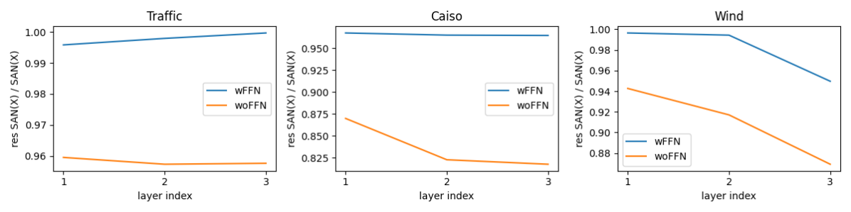
Figure 7. Relative norm of the residual along the depth for PatchTST with and without FFN

References

- (1)
- Bai et al. (2018) Shaojie Bai, J. Zico Kolter, and Vladlen Koltun. 2018. An Empirical Evaluation of Generic Convolutional and Recurrent Networks for Sequence Modeling. CoRR abs/1803.01271 (2018). arXiv:1803.01271 http://arxiv.org/abs/1803.01271
- Box and Jenkins (1968) G. E. P. Box and G. M. Jenkins. 1968. Some Recent Advances in Forecasting and Control. Journal of the Royal Statistical Society. Series C (Applied Statistics) 17, 2 (1968), 91–109.
- Dai et al. (2022) Damai Dai, Li Dong, Yaru Hao, Zhifang Sui, Baobao Chang, and Furu Wei. 2022. Knowledge Neurons in Pretrained Transformers. In Proceedings of the 60th Annual Meeting of the Association for Computational Linguistics (Volume 1: Long Papers), ACL 2022, Dublin, Ireland, May 22-27, 2022, Smaranda Muresan, Preslav Nakov, and Aline Villavicencio (Eds.). Association for Computational Linguistics, 8493–8502. https://doi.org/10.18653/V1/2022.ACL-LONG.581
- Devlin et al. (2019) Jacob Devlin, Ming-Wei Chang, Kenton Lee, and Kristina Toutanova. 2019. BERT: Pre-training of Deep Bidirectional Transformers for Language Understanding. In Proceedings of the 2019 Conference of the North American Chapter of the Association for Computational Linguistics: Human Language Technologies, Volume 1 (Long and Short Papers), Jill Burstein, Christy Doran, and Thamar Solorio (Eds.). Association for Computational Linguistics, Minneapolis, Minnesota, 4171–4186. https://doi.org/10.18653/v1/N19-1423
- Dosovitskiy et al. (2021) Alexey Dosovitskiy, Lucas Beyer, Alexander Kolesnikov, Dirk Weissenborn, Xiaohua Zhai, Thomas Unterthiner, Mostafa Dehghani, Matthias Minderer, Georg Heigold, Sylvain Gelly, Jakob Uszkoreit, and Neil Houlsby. 2021. An Image is Worth 16x16 Words: Transformers for Image Recognition at Scale. In International Conference on Learning Representations. https://openreview.net/forum?id=YicbFdNTTy
- Du et al. (2021) Yuntao Du, Jindong Wang, Wenjie Feng, Sinno Jialin Pan, Tao Qin, Renjun Xu, and Chongjun Wang. 2021. AdaRNN: Adaptive Learning and Forecasting of Time Series. Proceedings of the 30th ACM International Conference on Information & Knowledge Management (2021). https://api.semanticscholar.org/CorpusID:236966005
- Fan et al. (2023) Wei Fan, Pengyang Wang, Dongkun Wang, Dongjie Wang, Yuanchun Zhou, and Yanjie Fu. 2023. Dish-TS: A General Paradigm for Alleviating Distribution Shift in Time Series Forecasting. In Proceedings of the AAAI Conference on Artificial Intelligence, Vol. 37. 7522–7529.
- Ganin et al. (2016) Yaroslav Ganin, Evgeniya Ustinova, Hana Ajakan, Pascal Germain, Hugo Larochelle, François Laviolette, Mario Marchand, and Victor Lempitsky. 2016. Domain-Adversarial Training of Neural Networks. J. Mach. Learn. Res. 17, 1 (jan 2016), 2096–2030.
- Geva et al. (2020) Mor Geva, R. Schuster, Jonathan Berant, and Omer Levy. 2020. Transformer Feed-Forward Layers Are Key-Value Memories. ArXiv abs/2012.14913 (2020). https://api.semanticscholar.org/CorpusID:229923720
- Geva et al. (2021a) Mor Geva, Roei Schuster, Jonathan Berant, and Omer Levy. 2021a. Transformer Feed-Forward Layers Are Key-Value Memories. In Proceedings of the 2021 Conference on Empirical Methods in Natural Language Processing, Marie-Francine Moens, Xuanjing Huang, Lucia Specia, and Scott Wen-tau Yih (Eds.). Association for Computational Linguistics, Online and Punta Cana, Dominican Republic, 5484–5495. https://doi.org/10.18653/v1/2021.emnlp-main.446
- Geva et al. (2021b) Mor Geva, Roei Schuster, Jonathan Berant, and Omer Levy. 2021b. Transformer Feed-Forward Layers Are Key-Value Memories. In Proceedings of the 2021 Conference on Empirical Methods in Natural Language Processing. Association for Computational Linguistics, Online and Punta Cana, Dominican Republic, 5484–5495. https://doi.org/10.18653/v1/2021.emnlp-main.446
- Hochreiter and Schmidhuber (1997) Sepp Hochreiter and Jürgen Schmidhuber. 1997. Long Short-Term Memory. Neural Computation 9, 8 (Nov. 1997), 1735–1780.
- Hyndman and Athanasopoulos (2018) Robin John Hyndman and George Athanasopoulos. 2018. Forecasting: Principles and Practice (2nd ed.). OTexts, Australia.
- Kim et al. (2021) Taesung Kim, Jinhee Kim, Yunwon Tae, Cheonbok Park, Jang-Ho Choi, and Jaegul Choo. 2021. Reversible Instance Normalization for Accurate Time-Series Forecasting against Distribution Shift. In International Conference on Learning Representations.
- Kim et al. (2022) Taesung Kim, Jinhee Kim, Yunwon Tae, Cheonbok Park, Jang-Ho Choi, and Jaegul Choo. 2022. Reversible Instance Normalization for Accurate Time-Series Forecasting against Distribution Shift. In International Conference on Learning Representations. https://openreview.net/forum?id=cGDAkQo1C0p
- Kingma and Ba (2017) Diederik P. Kingma and Jimmy Ba. 2017. Adam: A Method for Stochastic Optimization. arXiv:1412.6980 [cs] (Jan. 2017). arXiv: 1412.6980.
- Kitaev et al. (2020) Nikita Kitaev, Lukasz Kaiser, and Anselm Levskaya. 2020. Reformer: The Efficient Transformer. In 8th International Conference on Learning Representations, ICLR 2020, Addis Ababa, Ethiopia, April 26-30, 2020.
- Lee et al. (2023) Daesoo Lee, Sara Malacarne, and Erlend Aune. 2023. Vector Quantized Time Series Generation with a Bidirectional Prior Model. In International Conference on Artificial Intelligence and Statistics. PMLR, 7665–7693.
- Lendasse et al. (2005) A. Lendasse, D. Francois, V. Wertz, and M. Verleysen. 2005. Vector quantization: a weighted version for time-series forecasting. Future Generation Computer Systems 21, 7 (2005), 1056–1067. https://doi.org/10.1016/j.future.2004.03.006
- Li et al. (2018) Haoliang Li, Sinno Jialin Pan, Shiqi Wang, and Alex C. Kot. 2018. Domain Generalization with Adversarial Feature Learning. In 2018 IEEE/CVF Conference on Computer Vision and Pattern Recognition. 5400–5409. https://doi.org/10.1109/CVPR.2018.00566
- Li et al. (2022) Yan Li, Xinjiang Lu, Yaqing Wang, and Dejing Dou. 2022. Generative Time Series Forecasting with Diffusion, Denoise, and Disentanglement. In Advances in Neural Information Processing Systems, Alice H. Oh, Alekh Agarwal, Danielle Belgrave, and Kyunghyun Cho (Eds.). https://openreview.net/forum?id=rG0jm74xtx
- Lin et al. (2023) Shengsheng Lin, Weiwei Lin, Wentai Wu, Songbo Wang, and Yongxiang Wang. 2023. PETformer: Long-term Time Series Forecasting via Placeholder-enhanced Transformer. arXiv:2308.04791 [cs.LG]
- Liu et al. (2022) Shizhan Liu, Hang Yu, Cong Liao, Jianguo Li, Weiyao Lin, Alex X Liu, and Schahram Dustdar. 2022. Pyraformer: Low-Complexity Pyramidal Attention for Long-Range Time Series Modeling and Forecasting. In International Conference on Learning Representations.
- Lu et al. (2022) Wang Lu, Jindong Wang, Haoliang Li, Yiqiang Chen, and Xing Xie. 2022. Domain-invariant Feature Exploration for Domain Generalization. Trans. Mach. Learn. Res. 2022 (2022). https://api.semanticscholar.org/CorpusID:249172563
- Lu et al. (2023) Wang Lu, Jindong Wang, Xinwei Sun, Yiqiang Chen, and Xing Xie. 2023. Out-of-distribution Representation Learning for Time Series Classification. In The Eleventh International Conference on Learning Representations. https://openreview.net/forum?id=gUZWOE42l6Q
- Makridakis et al. (2018) Spyros Makridakis, Evangelos Spiliotis, and Vassilios Assimakopoulos. 2018. The M4 Competition: Results, findings, conclusion and way forward. International Journal of Forecasting (2018). https://api.semanticscholar.org/CorpusID:158696437
- Muandet et al. (2013) Krikamol Muandet, David Balduzzi, and Bernhard Schölkopf. 2013. Domain Generalization via Invariant Feature Representation. In Proceedings of the 30th International Conference on Machine Learning (Proceedings of Machine Learning Research, Vol. 28), Sanjoy Dasgupta and David McAllester (Eds.). PMLR, Atlanta, Georgia, USA, 10–18. https://proceedings.mlr.press/v28/muandet13.html
- Nie et al. (2022) Yuqi Nie, Nam H. Nguyen, Phanwadee Sinthong, and Jayant Kalagnanam. 2022. A Time Series is Worth 64 Words: Long-term Forecasting with Transformers. CoRR abs/2211.14730 (2022). https://doi.org/10.48550/arXiv.2211.14730 arXiv:2211.14730
- Ogasawara et al. (2010) Eduardo Ogasawara, Leonardo C. Martinez, Daniel de Oliveira, Geraldo Zimbrão, Gisele L. Pappa, and Marta Mattoso. 2010. Adaptive Normalization: A novel data normalization approach for non-stationary time series. In The 2010 International Joint Conference on Neural Networks (IJCNN). 1–8. https://doi.org/10.1109/IJCNN.2010.5596746
- Oreshkin et al. (2019) Boris N Oreshkin, Dmitri Carpov, Nicolas Chapados, and Yoshua Bengio. 2019. N-BEATS: Neural basis expansion analysis for interpretable time series forecasting. In Proceedings of the International Conference on Learning Representations (ICLR).
- Passalis et al. (2019) Nikolaos Passalis, Anastasios Tefas, Juho Kanniainen, M. Gabbouj, and Alexandros Iosifidis. 2019. Deep Adaptive Input Normalization for Time Series Forecasting. IEEE Transactions on Neural Networks and Learning Systems 31 (2019), 3760–3765. https://api.semanticscholar.org/CorpusID:202719461
- Qin et al. (2017) Yao Qin, Dongjin Song, Haifeng Chen, Wei Cheng, Guofei Jiang, and Garrison W. Cottrell. 2017. A Dual-Stage Attention-Based Recurrent Neural Network for Time Series Prediction. In Proceedings of the Twenty-Sixth International Joint Conference on Artificial Intelligence (IJCAI), Melbourne, Australia, August 19-25, 2017. ijcai.org, 2627–2633.
- Rao et al. (2021) Yongming Rao, Wenliang Zhao, Zheng Zhu, Jiwen Lu, and Jie Zhou. 2021. Global Filter Networks for Image Classification. In Advances in Neural Information Processing Systems, A. Beygelzimer, Y. Dauphin, P. Liang, and J. Wortman Vaughan (Eds.). https://openreview.net/forum?id=K_Mnsw5VoOW
- Rasul et al. (2022) Kashif Rasul, Young-Jin Park, Max Nihlén Ramström, and KyungHyun Kim. 2022. VQ-AR: Vector Quantized Autoregressive Probabilistic Time Series Forecasting. ArXiv abs/2205.15894 (2022). https://api.semanticscholar.org/CorpusID:249210148
- Salinas et al. (2020) David Salinas, Valentin Flunkert, Jan Gasthaus, and Tim Januschowski. 2020. DeepAR: Probabilistic forecasting with autoregressive recurrent networks. International Journal of Forecasting 36, 3 (2020), 1181–1191.
- Shao et al. (2023) Zezhi Shao, Fei Wang, Yongjun Xu, Wei Wei, Chengqing Yu, Zhao Zhang, Di Yao, Guangyin Jin, Xin Cao, Gao Cong, Christian S. Jensen, and Xueqi Cheng. 2023. Exploring Progress in Multivariate Time Series Forecasting: Comprehensive Benchmarking and Heterogeneity Analysis. arXiv:2310.06119 [cs.LG]
- Shin et al. (2021) Won Young Shin, Gyubok Lee, Jiyoung Lee, Eun-Young Lyou, Joonseok Lee, and E. Choi. 2021. Exploration Into Translation-Equivariant Image Quantization. ICASSP 2023 - 2023 IEEE International Conference on Acoustics, Speech and Signal Processing (ICASSP) (2021), 1–5. https://api.semanticscholar.org/CorpusID:257038529
- Tao et al. (2020) Zhulin Tao, Xiang Wang, Xiangnan He, Xianglin Huang, and Tat-Seng Chua. 2020. HoAFM: A High-order Attentive Factorization Machine for CTR Prediction. Information Processing Management 57, 6 (2020), 102076. https://doi.org/10.1016/j.ipm.2019.102076
- Taylor and Letham (2018) Sean J. Taylor and Benjamin Letham. 2018. Forecasting at Scale. The American Statistician 72 (2018), 37 – 45. https://api.semanticscholar.org/CorpusID:12515984
- Tzeng et al. (2017) Eric Tzeng, Judy Hoffman, Kate Saenko, and Trevor Darrell. 2017. Adversarial Discriminative Domain Adaptation. In 2017 IEEE Conference on Computer Vision and Pattern Recognition (CVPR). 2962–2971. https://doi.org/10.1109/CVPR.2017.316
- van den Oord et al. (2017) Aäron van den Oord, Oriol Vinyals, and Koray Kavukcuoglu. 2017. Neural Discrete Representation Learning. In Advances in Neural Information Processing Systems 30: Annual Conference on Neural Information Processing Systems 2017, December 4-9, 2017, Long Beach, CA, USA, Isabelle Guyon, Ulrike von Luxburg, Samy Bengio, Hanna M. Wallach, Rob Fergus, S. V. N. Vishwanathan, and Roman Garnett (Eds.). 6306–6315. https://proceedings.neurips.cc/paper/2017/hash/7a98af17e63a0ac09ce2e96d03992fbc-Abstract.html
- Vaswani et al. (2017) Ashish Vaswani, Noam Shazeer, Niki Parmar, Jakob Uszkoreit, Llion Jones, Aidan N Gomez, Łukasz Kaiser, and Illia Polosukhin. 2017. Attention is all you need. Advances in neural information processing systems 30 (2017).
- Wang et al. (2023) Huiqiang Wang, Jian Peng, Feihu Huang, Jince Wang, Junhui Chen, and Yifei Xiao. 2023. MICN: Multi-scale Local and Global Context Modeling for Long-term Series Forecasting. In The Eleventh International Conference on Learning Representations. https://openreview.net/forum?id=zt53IDUR1U
- Wang et al. (2018) Jindong Wang, Wenjie Feng, Yiqiang Chen, Han Yu, Meiyu Huang, and Philip S. Yu. 2018. Visual Domain Adaptation with Manifold Embedded Distribution Alignment. In Proceedings of the 26th ACM International Conference on Multimedia (Seoul, Republic of Korea) (MM ’18). Association for Computing Machinery, New York, NY, USA, 402–410. https://doi.org/10.1145/3240508.3240512
- Wang et al. (2021) Jindong Wang, Cuiling Lan, Chang Liu, Yidong Ouyang, and Tao Qin. 2021. Generalizing to Unseen Domains: A Survey on Domain Generalization. IEEE Transactions on Knowledge and Data Engineering 35 (2021), 8052–8072. https://api.semanticscholar.org/CorpusID:232110832
- Wen et al. (2022) Qingsong Wen, Tian Zhou, Chaoli Zhang, Weiqi Chen, Ziqing Ma, Junchi Yan, and Liang Sun. 2022. Transformers in Time Series: A Survey. arXiv preprint arXiv:2202.07125 (2022).
- Wu et al. (2022) Haixu Wu, Tengge Hu, Yong Liu, Hang Zhou, Jianmin Wang, and Mingsheng Long. 2022. TimesNet: Temporal 2D-Variation Modeling for General Time Series Analysis. CoRR abs/2210.02186 (2022). https://doi.org/10.48550/arXiv.2210.02186 arXiv:2210.02186
- Wu et al. (2021) Haixu Wu, Jiehui Xu, Jianmin Wang, and Mingsheng Long. 2021. Autoformer: Decomposition transformers with auto-correlation for long-term series forecasting. In Proceedings of the Advances in Neural Information Processing Systems (NeurIPS). 101–112.
- Yu et al. (2022a) Jiahui Yu, Xin Li, Jing Yu Koh, Han Zhang, Ruoming Pang, James Qin, Alexander Ku, Yuanzhong Xu, Jason Baldridge, and Yonghui Wu. 2022a. Vector-quantized Image Modeling with Improved VQGAN. In The Tenth International Conference on Learning Representations, ICLR 2022, Virtual Event, April 25-29, 2022. OpenReview.net. https://openreview.net/forum?id=pfNyExj7z2
- Yu et al. (2022b) Jiahui Yu, Xin Li, Jing Yu Koh, Han Zhang, Ruoming Pang, James Qin, Alexander Ku, Yuanzhong Xu, Jason Baldridge, and Yonghui Wu. 2022b. Vector-quantized Image Modeling with Improved VQGAN. In The Tenth International Conference on Learning Representations, ICLR 2022, Virtual Event, April 25-29, 2022. OpenReview.net. https://openreview.net/forum?id=pfNyExj7z2
- Zeghidour et al. (2022) Neil Zeghidour, Alejandro Luebs, Ahmed Omran, Jan Skoglund, and Marco Tagliasacchi. 2022. SoundStream: An End-to-End Neural Audio Codec. IEEE ACM Trans. Audio Speech Lang. Process. 30 (2022), 495–507. https://doi.org/10.1109/TASLP.2021.3129994
- Zeng et al. (2022) Ailing Zeng, Muxi Chen, Lei Zhang, and Qiang Xu. 2022. Are Transformers Effective for Time Series Forecasting? CoRR abs/2205.13504 (2022). https://doi.org/10.48550/arXiv.2205.13504 arXiv:2205.13504
- Zhao et al. (2023) Yanjun Zhao, Ziqing‘ Ma, Tian Zhou, Mengni Ye, Liang Sun, and Yi Qian. 2023. GCformer: An Efficient Solution for Accurate and Scalable Long-Term Multivariate Time Series Forecasting. In Proceedings of the 32nd ACM International Conference on Information and Knowledge Management (<conf-loc>, <city>Birmingham</city>, <country>United Kingdom</country>, </conf-loc>) (CIKM ’23). Association for Computing Machinery, New York, NY, USA, 3464–3473. https://doi.org/10.1145/3583780.3615136
- Zhou et al. (2021) Haoyi Zhou, Shanghang Zhang, Jieqi Peng, Shuai Zhang, Jianxin Li, Hui Xiong, and Wancai Zhang. 2021. Informer: Beyond Efficient Transformer for Long Sequence Time-Series Forecasting. In The Thirty-Fifth AAAI Conference on Artificial Intelligence, AAAI 2021, Virtual Conference, Vol. 35. 11106–11115.
- Zhou et al. (2022a) Tian Zhou, Ziqing Ma, Qingsong Wen, Xue Wang, Liang Sun, and Rong Jin. 2022a. FEDformer: Frequency enhanced decomposed transformer for long-term series forecasting. In 39th International Conference on Machine Learning (ICML).
- Zhou et al. (2022b) Tian Zhou, Ziqing Ma, xue wang, Qingsong Wen, Liang Sun, Tao Yao, Wotao Yin, and Rong Jin. 2022b. FiLM: Frequency improved Legendre Memory Model for Long-term Time Series Forecasting. In Advances in Neural Information Processing Systems, Alice H. Oh, Alekh Agarwal, Danielle Belgrave, and Kyunghyun Cho (Eds.). https://openreview.net/forum?id=zTQdHSQUQWc
- Zhou et al. (2023) Tian Zhou, Peisong Niu, Xue Wang, Liang Sun, and Rong Jin. 2023. One Fits All: Power General Time Series Analysis by Pretrained LM. In NeurIPS.