Microscopic models for the large-scale spread of SARS-CoV-2 virus: A Statistical Mechanics approach

Abstract

In this work, we derive a system of Boltzmann-type equations to describe the spread of SARS-CoV-2 virus at the microscopic scale, that is by modeling the human-to-human mechanisms of transmission. To this end, we consider two populations, characterized by specific distribution functions, made up of individuals without symptoms (population $1$) and infected people with symptoms (population $2$). The Boltzmann operators model the interactions between individuals within the same population and among different populations with a probability of transition from one to the other due to contagion or, vice versa, to recovery. In addition, the influence of innate and adaptive immune systems is taken into account. Then, starting from the Boltzmann microscopic description we derive a set of evolution equations for the size and mean state of each population considered. Mathematical properties of such macroscopic equations, as equilibria and their stability, are investigated and some numerical simulations are performed in order to analyze the ability of our model to reproduce the characteristic features of Covid-19.

Keywords: Boltzmann equation, kinetic theory, epidemiological models, living systems, nonlinearity

Mathematics Subject Classification: 35Q20, 82C40, 92D30

1 Introduction

The history of mathematical models in epidemiology begins with the paper ”Essai d’une nouvelle analyse de la mortalité causée par la petite vérole” written by Daniel Bernoulli in $1766$ to analyze the mortality due to smallpox in England [2]. In this paper, Bernoulli derived a model showing that inoculation against the virus would increase the life expectancy. Following the work of Bernoulli, Lambert in $1772$ extended the model by incorporating age-dependent parameters [15]. However, this kind of approach has not been developed systematically until $1911$ when the British medical doctor Ronald Ross published the paper ”The prevention of malaria”, considered the starting point of the modern mathematical epidemiology [18]. For the first time, in this work, a set of differential equations were derived to study the discrete-time dynamics of mosquito-borne malaria. Similar epidemic models were later developed by Kermack and McKendrick, who founded the deterministic compartmental modeling [12, 13, 14]. These authors proposed the celebrated SIR model according to which the population is divided into three groups or compartments: the susceptible (S), who can contract the disease, the infected (I), who have already contracted the disease and can transmit it, and the recovered (R), who are healed. Within this framework, it is assumed that the probability of infection of a susceptible is proportional to the number of its contacts with infected individuals. The resulting mathematical model, based on a deterministic system of ordinary differential equations, relies on the following hypotheses: (i) a homogeneous mixing of the contacts; (ii) the conservation of the total population; (iii) relatively low rates of interaction. Over the years, SIR-type models have been extended to include age-dependent infection, mortality and spatial dependence of the epidemic spread [20], [26], [27].

However, since the classical epidemiological models are derived at a macroscopic level, they neglect the heterogeneity of disease transmission due to the microscopic features of the interactions between individuals. Relying on recent developments of kinetic models for the description of social and economic phenomena [9, 22], in the last few years a number of works have appeared aimed to connect the distribution of social contacts with the spreading of a disease in a multi-agent system [17]. This issue has been carried out by integrating a classical compartmental model (typically a SIR-type model) with a statistical part based on Boltzmann-like equations describing the formation of social contacts. Such an approach allows one to obtain various sub-classes of macroscopic epidemiological models characterized by non-linear incidence rates. Within the same mathematical framework of multi-agent systems, a different procedure has been considered in [8], where kinetic evolution equations have been derived for the distribution functions of the viral load of the individuals, that change as a consequence of binary interactions or interactions with a background. But also in this case a SIR-like compartmental structure has been taken into account in order to describe the health status of individuals.

In the present paper, following the general setting put forward in [6, 7], we derive a system of Boltzmann-type evolution equations for the distribution function $f_{i}(t,u_{i})$ ($i=1,2$) of two interacting populations, where the index $i=1$ refers to individuals without symptoms and $i=2$ to infected people with symptoms. Unlike the kinetic models mentioned above, in our work the microscopic variable $u_{i}\in(-\infty,+\infty)$ indicates the level of the infection, so that the product $f_{i}(t,u_{i})\,du_{i}$ gives the number of individuals of the $i$-th population which at the time $t$ are in the elementary state $[u_{i},u_{i}+du_{i}]$. Within the population described by the distribution function $f_{1}(t,u_{1})$ we can distinguish healthy individuals, when $u_{1}<0$, and positive asymptomatic, when $u_{1}\geq 0$. Similarly, the population represented by the distribution function $f_{2}(t,u_{2})$ is made up of positive symptomatic, when $u_{2}<0$, and hospitalized individuals, when $u_{2}\geq 0$. Our approach does not rely on one of the existing compartmental models, but starting from a microscopic description of the interactions between individuals based on the Boltzmann equation, we derive a new class of macroscopic models, which account for the peculiarities of Covid-19 spread. The idea behind our derivation is to treat interactions between individuals in the same way as those between molecules of chemically reacting gas mixtures. In particular, the transition from population $1$ (made up of individuals without symptoms) to population $2$ (made up of infected individuals with symptoms) is described by using the same formalism of reversible chemical reactions in kinetic theory of gases. The reverse ’chemical reaction’ is taken into account when the medical staff (belonging to population $1$) ’interacts’ with positive symptomatic or with people hospitalized (belonging to population $2$) giving rise to their recovery. We also consider the action of the immune system modeled in close analogy to the interaction of a particle (a single person) with a background (the immune system), typical of the neutron transport description in kinetic theory [5]. The major mathematical difficulty in our model consists in deriving a system of four macroscopic equations for the evolution of the number densities and mean states of healthy people, positive asymptomatic, positive symptomatic and hospitalized persons, starting from a set of two Boltzmann equations defined at the microscopic level for the distribution functions $f_{1}$ and $f_{2}$. The closure of such macroscopic system is based on specific choices of Boltzmann collision kernels and of interaction rules that, as usual in multi-agent systems involving human beings, also show stochastic effects.

The rest of the paper is organized as follows. In Section 2 we present the epidemiological model derived at the microscopic level by setting a system of Boltzmann-like equations. In Sections 3 and 4 we obtain the macrocopic equations for the evolution of the size and mean state, respectively, of each population considered, that is healthy individuals, positive asymptomatic, positive symptomatic and hospitalized individuals. These macroscopic equations are then qualitatively analyzed. In particular, the equilibrium states and their stability are investigated in Sections 5 and 6, respectively. Section 7 presents numerical test cases carried out in order to analyze the ability of our model to reproduce the characteristic features of Covid-19. Some concluding remarks, mainly aimed at highlighting the novelty of our approach, are included in Section 8. Finally, in Appendix A we introduce some preliminaries on the scattering kernel formulation of the Boltzmann equation used in this paper, while Appendix B is devoted to summarize the main features of the classical kinetic approach to chemically reacting gas mixtures.

2 Mathematical formulation

We derive a model describing the spread of SARS-CoV-2 virus within the general mathematical framework of the kinetic theory for chemically reacting mixtures of gases [19]. The system consists of two populations of interacting individuals. Each population is denoted by the subscript $i$ ($i=1,2$), according to the following classification:

$$\left\{\begin{array}[]{rl}i=1:&\text{individuals without symptoms}\\ i=2:&\text{infected individuals with symptoms.}\end{array}\right.$$ (1)

Within the same population, each individual is characterized by a microscopic state, which is a scalar variable $u_{i}\in(-\infty,+\infty)$ (activity) [6], [7]. Let us introduce the one-particle distribution function: $f_{i}=f_{i}(t,u_{i})$. By definition, the product

$$f_{i}(t,u_{i})\,du_{i}$$

gives the number of individuals of the $i$-th population which at the time $t$ are in the elementary state $[u_{i},u_{i}+du_{i}]$. The variable $u_{i}$ depends on the intensity level of a certain pathological state. We distinguish the following cases:

$$f_{1}(t,u_{1}):\left\{\begin{array}[]{rl}\text{if}\,u_{1}<0&\rightarrow\text{healthy-individuals}\\ \text{if}\,u_{1}\geq 0&\rightarrow\text{positive-asymptomatic}\end{array}\right.$$ (2)

$$f_{2}(t,u_{2}):\left\{\begin{array}[]{rl}\text{if}\,u_{2}<0&\rightarrow\text{positive-symptomatic}\\ \text{if}\,u_{2}\geq 0&\rightarrow\text{hospitalized-individuals}.\end{array}\right.$$ (3)

Specifically, within the same population, the larger is the value of $u_{i}$, the stronger is the infection.

The evolution of the system is determined by microscopic interactions between pairs of individuals, which modify the probability distribution over the state variable and/or the size of the population. The system is homogeneous in space and only binary interactions are taken into account. In addition, we model also the action of the immune system described by the distribution function $\phi_{i}(v)\;\;(i=1,2)$ over the microscopic variable $v\in[-M,+M]$, where $M$ is a constant such that $M>>1$. The immune response to SARS-CoV-2 virus is unpredictable and very different from person to person. We distinguish between two natural actions:

(i) The innate immunity.

Bacteria or viruses that enter the body can be stopped right away by the innate immune system. The effectiveness of this type of action is linked to the possibility that an individual belonging to population $1$ becomes ill or not.

(ii) The adaptive immunity.

The adaptive immune system takes over if the innate immune system is not able to destroy the germs. It is slower to respond than the innate immune system, but it identifies the germs and it is able to ’remember’ them. To the adaptive immunity can be ascribed the recovery of an individual belonging to population $2$ even in the absence of specific care. The current knowledge about SARS-CoV-2 infection indicates that the immune system plays a crucial role in setting the severity of Covid-19. Appropriate immune responses against SARS-CoV-2 could mitigate the symptoms of Covid-19 and prevent the occurrence of a severe disease, while excessive responses trigger pathogenic cell activation increasing the risk of death.

We will consider the following moments of the distribution functions.

(a) The size of the $i$th population at time $t$:

$$n_{i}(t)=\int_{-\infty}^{+\infty}f_{i}(t,u_{i})\,du_{i},\;\;\;\;i=1,2$$ (4)

where $n_{1}=n_{1}^{HE}+n_{1}^{A}$ and $n_{2}=n_{2}^{S}+n_{2}^{HS}$, with

$$n_{1}^{HE}=\int_{-\infty}^{0}f_{1}(t,u_{1})\,du_{1}:\;\;\text{number density of healthy individuals}$$ (5)

$$n_{1}^{A}=\int_{0}^{+\infty}f_{1}(t,u_{1})\,du_{1}:\;\;\text{number density of asymptomatic}$$ (6)

$$n_{2}^{S}=\int_{-\infty}^{0}f_{2}(t,u_{2})\,du_{2}:\;\;\text{number density of symptomatic}$$ (7)

$$n_{2}^{HS}=\int_{0}^{+\infty}f_{2}(t,u_{2})\,du_{2}:\;\;\text{number density of hospitalized individuals}.$$ (8)

The total number of individuals at time $t$ is given by:

$$N=\sum_{i=1}^{2}n_{i}(t).$$ (9)

Since in this work we are mainly interested in modeling the transmission mechanism of the disease, we will neglect changes in the social structure such as the aging process, births, and deaths. This conservation property implies that $N$ is a constant.

Furthermore, the overall action of the immune system on the individuals of the $i$th population is given by

$$\hat{I}_{i}=\int_{-M}^{+M}\phi_{i}(v)\,dv,\;\;\;\;i=1,2.$$ (10)

Higher-order moments provide additional information on the (macroscopic) description of the system.

(b) Progression of the epidemiological state:

$$U_{i}(t)=\int_{-\infty}^{+\infty}u_{i}\,f_{i}(t,u_{i})\,du_{i}\;\;\;\;i=1,2.$$ (11)

The evolution equations for the distribution functions $f_{i}(t,u_{i})$ can be obtained following the formalism of the Boltzmann equations for chemically reacting gas mixtures (see Appendix B). In order to derive these equations, we consider the following hypotheses on interaction processes:

(H.1) the medical staff belongs to the population $1$, with $u_{1}\in[-\infty,0[$, and never becomes positive-asymptomatic or ill when interacting with sick people belonging to population $2$;

(H.2) the interactions produce a smooth shift towards higher pathological states (e.g., a healthy person does not immediately become ill but positive-asymptomatic);

(H.3) all positive-symptomatic individuals are in isolation and, therefore, they can only have interactions with family members (also positive-symptomatic) and with the medical staff;

(H.4) hospitalized-individuals can only have interactions between themselves and with the medical staff.

Relying on these assumptions, we describe the interactions within the same population or between different populations as follows.

• Interactions within the population $1$.

  (a) Healthy-individuals + healthy-individuals
  $\longrightarrow$ both individuals remain healthy (population $1$);

  (b) healthy-individuals + positive-asymptomatic:
  besides the interactions in which individuals do not change category, it may occur the transition healthy-individual $\longrightarrow$ positive-asymptomatic (population $1$);

  (c) positive-asymptomatic + positive-asymptomatic:
  it could happen that both remain positive-asymptomatic, or that one undergoes the transition positive-asymptomatic $\longrightarrow$ positive-symptomatic (population $2$).

• Interactions within the population $2$.

  (d) Positive-symptomatic + positive-symptomatic:
  one of them could be subject to the change positive-symptomatic $\longrightarrow$ hospitalized-individual (population $2$);

  (e) hospitalized-individuals + hospitalized-individuals:
  $\longrightarrow$ both individuals remain hospitalized (population $2$).

• Interactions between the populations $1$ and $2$.
  Only the medical staff interacts with positive symptomatic or with hospitalized people. Besides ’elastic’ encounters, where the ill individuals do not change their category, we have the following interactions giving rise to recovery:

  (f) Healthy-individual (medical staff) + positive-symptomatic $\longrightarrow$ healthy-individuals (transition to population $1$);

  (g) healthy-individual (medical staff) + hospitalized-individuals $\longrightarrow$ healthy-individuals (transition to population $1$).

Therefore, we shall deal with a ’mixture’ of two populations $(1,2)$ which can interact according to the following reversible ’chemical reaction’:

$$1+1\rightleftarrows 2+1$$ (12)

In addition to the interactions between individuals, we consider also those between an individual and the immune system, modeled in close analogy to the interaction of a particle with a background, typical of the neutron transport phenomena in kinetic theory [5]. In particular, we assume that among the individuals in population $1$, only asymptomatic carriers ’interact’ with their innate immune system with the probability to become positive symptomatic (transition to population $2$). Furthermore, we assume that people belonging to population $2$ (both positive symptomatic and hospitalized individuals) interact with their adaptive immune system with a probability of recovery (transition to population $1$ among healthy individuals). While the interactions between individuals are described by the full nonlinear Boltzmann operator, those between a person and the immune system give rise to a linear collision operator.

2.1 Derivation of Boltzmann-type equations

In the following, we consider the scattering kernel formulation of the Boltzmann collision operator (see Appendix A) for both ’elastic’ ($Q_{ik}$) and ’chemical’ interactions ($\overline{Q}_{i}^{(r)}$, $\overline{L}_{i}^{(r)}$). In particular, the operators $Q_{ii}$ ($i=1,2$) describe the interactions between individuals within the same population $i$ without a transfer to the other population; the operators $Q_{12}$ and $Q_{21}$ model the interactions between the medical staff (belonging to population $1$) and sick people (belonging to population $2$) which do not produce any change of category, while the operators $\overline{Q}_{i}^{(r)}$ account for those interactions between individuals which give rise to a transition from one population to the other; finally, the operators $\overline{L}_{i}^{(r)}$ take into account the interactions of persons belonging to population $i$ with the immune system.

Thus, we get for population $1$:

$$\frac{\partial f_{1}}{\partial t}(t,u_{1})=Q_{11}+Q_{12}+\overline{Q}_{1}^{(r)}+\overline{L}_{1}^{(r)}$$ (13)

where

$$Q_{11}= \displaystyle\int_{-\infty}^{+\infty}\int_{-\infty}^{+\infty}\eta_{11}(u_{*},u^{*})\,A_{11}^{(1)}(u_{*},u^{*};u_{1})f_{1}(t,u_{*})\,f_{1}(t,u^{*})\,du_{*}\,du^{*}$$ (14)

$$-f_{1}(t,u_{1})\displaystyle\int_{-\infty}^{+\infty}\eta_{11}(u_{1},u^{*})\,f_{1}(t,u^{*})\,du^{*}$$

$$Q_{12}= \displaystyle\int_{-\infty}^{+\infty}\int_{-\infty}^{+\infty}\eta_{12}(u_{*},u^{*})\,A_{12}^{(1)}(u_{*},u^{*};u_{1})f_{1}(t,u_{*})\,f_{2}(t,u^{*})\,du_{*}\,du^{*}$$ (15)

$$-f_{1}(t,u_{1})\displaystyle\int_{-\infty}^{+\infty}\eta_{12}(u_{1},u^{*})\,f_{2}(t,u^{*})\,du^{*}$$

$$\overline{Q}_{1}^{(r)}= \displaystyle\int_{-\infty}^{+\infty}\int_{-\infty}^{+\infty}\eta_{11}^{(r)}(u_{*},u^{*})\,{\tilde{A}}_{11}^{(1)}(u_{*},u^{*};u_{1})f_{1}(t,u_{*})\,f_{1}(t,u^{*})\,du_{*}\,du^{*}$$ (16)

$$-2f_{1}(t,u_{1})\displaystyle\int_{-\infty}^{+\infty}\eta_{11}^{(r)}(u_{1},u^{*})\,f_{1}(t,u^{*})\,du^{*}$$

$$+2\displaystyle\int_{-\infty}^{+\infty}du_{*}\int_{-\infty}^{+\infty}\eta_{21}^{(r)}(u_{*},u^{*})\,{\tilde{A}}_{21}^{(1)}(u_{*},u^{*};u_{1})f_{2}(t,u_{*})\,f_{1}(t,u^{*})\,du^{*}$$

$$-f_{1}(t,u_{1})\displaystyle\int_{-\infty}^{+\infty}\eta_{21}^{(r)}(u_{1},u^{*})\,f_{2}(t,u^{*})\,du^{*}$$

$$\overline{L}_{1}^{(r)}= \displaystyle\int_{-\infty}^{+\infty}du_{*}\int_{-M}^{+M}\mu_{2}^{(r)}(u_{*},v^{*})\,B_{2}^{(1)}(u_{*},v^{*};u_{1})f_{2}(t,u_{*})\,\phi_{2}(v^{*})\,dv^{*}$$ (17)

$$-f_{1}(t,u_{1})\displaystyle\int_{-M}^{+M}\mu_{1}^{(r)}(u_{1},v^{*})\,\phi_{1}(v^{*})\,dv^{*}$$

Likewise, we can write for population $2$:

$$\frac{\partial f_{2}}{\partial t}(t,u_{2})=Q_{22}+Q_{21}+\overline{Q}_{2}^{(r)}+\overline{L}_{2}^{(r)}$$ (18)

where

$$Q_{22}= \displaystyle\int_{-\infty}^{+\infty}\int_{-\infty}^{+\infty}\eta_{22}(u_{*},u^{*})\,A_{22}^{(2)}(u_{*},u^{*};u_{2})f_{2}(t,u_{*})\,f_{2}(t,u^{*})\,du_{*}\,du^{*}$$ (19)

$$-f_{2}(t,u_{2})\displaystyle\int_{-\infty}^{+\infty}\eta_{22}(u_{2},u^{*})\,f_{2}(t,u^{*})\,du^{*}$$

$$Q_{21}= \displaystyle\int_{-\infty}^{+\infty}\int_{-\infty}^{+\infty}\eta_{21}(u_{*},u^{*})\,A_{21}^{(2)}(u_{*},u^{*};u_{2})f_{2}(t,u_{*})\,f_{1}(t,u^{*})\,du_{*}\,du^{*}$$ (20)

$$-f_{2}(t,u_{2})\displaystyle\int_{-\infty}^{+\infty}\eta_{21}(u_{2},u^{*})\,f_{1}(t,u^{*})\,du^{*}$$

$$\overline{Q}_{2}^{(r)}= \displaystyle\int_{-\infty}^{+\infty}\int_{-\infty}^{+\infty}\eta_{11}^{(r)}(u_{*},u^{*})\,{\tilde{A}}_{11}^{(2)}(u_{*},u^{*};u_{2})f_{1}(t,u_{*})\,f_{1}(t,u^{*})\,du_{*}\,du^{*}$$ (21)

$$-f_{2}(t,u_{2})\displaystyle\int_{-\infty}^{+\infty}\eta_{21}^{(r)}(u_{2},u^{*})\,f_{1}(t,u^{*})\,du^{*}$$

$$\overline{L}_{2}^{(r)}= \displaystyle\int_{-\infty}^{+\infty}du_{*}\int_{-M}^{+M}\mu_{1}^{(r)}(u_{*},v^{*})\,B_{1}^{(2)}(u_{*},v^{*};u_{2})f_{1}(t,u_{*})\,\phi_{1}(v^{*})\,dv^{*}$$ (22)

$$-f_{2}(t,u_{2})\displaystyle\int_{-M}^{+M}\mu_{2}^{(r)}(u_{2},v^{*})\,\phi_{2}(v^{*})\,dv^{*}.$$

In the above equations, $\eta_{hk}$ (and $\eta_{hk}^{(r)}$) is called encounter rate and it describes the rate of interactions (that is, the number of encounters per unit time) between individuals of the $h$-th population and individuals of the $k$-th population, while $\mu_{h}^{(r)}$ refers to the rate of interaction between individuals of the $h$-th population and the immune system. To construct the transition rates, we assume that the interactions between individuals can be modeled in analogy to the intermolecular potentials acting between the gas molecules. Since in the framework of kinetic theory of rarefied gases analytical manipulations can be carried out in closed form for Maxwell molecules (see Appendix A) [5], we restrict ourselves to this kind of interaction, which leads to assume $\eta_{hk}$ constant. In particular, when the encounters between individuals belonging to different groups are forbidden, in the framework of our epidemiological model, the rates $\eta_{hk}$ vanish. Thus, for the elastic operator $Q_{11}$, since all types of interactions between healthy and positive–asymptomatic people are allowed, we set

$$\eta_{11}(u_{*},u^{*})=\bar{\eta}_{11}\qquad\quad\forall\,\,u_{*}\in\mathbb{R},\quad u^{*}\in\mathbb{R}.$$

In the operator $Q_{22}$, since positive–symptomatic individuals cannot interact with hospitalized people, we have

$$\eta_{22}(u_{*},u^{*})=\left\{\begin{array}[]{ll}\bar{\eta}_{22}&\text{if}\ (u_{*}<0,u^{*}<0)\ \text{or}\ (u_{*}>0,u^{*}>0)\\ 0&\text{otherwise}\end{array}\right.$$

The interactions between the two populations $1$ and $2$ describe only the possible contacts between the ill individuals and the medical staff (healthy), therefore

$$\eta_{12}(u_{*},u^{*})=\left\{\begin{array}[]{ll}\bar{\eta}_{12}&\text{if}\ u_{*}<0\quad\text{in}\ f_{1}(t,u_{*})\\ 0&\text{otherwise}\end{array}\right.$$

$$\eta_{21}(u_{*},u^{*})=\left\{\begin{array}[]{ll}\bar{\eta}_{21}&\text{if}\ u^{*}<0\quad\text{in}\ f_{1}(t,u^{*})\\ 0&\text{otherwise}\end{array}\right.$$

and moreover, since both rates refer to the same type of interactions, we assume

$$\bar{\eta}_{12}=\bar{\eta}_{21}\,.$$

For the direct transition $1+1\rightarrow 2+1$, that can occur when two positive-asymptomatic individuals interact, we set

$$\eta_{11}^{(r)}(u_{*},u^{*})=\left\{\begin{array}[]{ll}\bar{\eta}_{11}^{(r)}&\text{if}\ u_{*}>0\ \text{and}\ u^{*}>0\\ 0&\text{otherwise}\end{array}\right.$$

For the reverse interaction $2+1\rightarrow 1+1$, taking into account that population $2$ may interact only with the medical staff we have

$$\eta_{21}^{(r)}(u_{*},u^{*})=\left\{\begin{array}[]{ll}\bar{\eta}_{21}^{(r)}&\text{if}\ u^{*}<0\quad\text{in}\ f_{1}(t,u^{*})\\ 0&\text{otherwise}\end{array}\right.$$

The interactions with the immune system involve the positive-asymptomatic persons in population $1$ and all the individuals in population $2$; for this reason we set

$$\mu_{1}^{(r)}(u_{*},v^{*})=\left\{\begin{array}[]{ll}\bar{\mu}_{1}^{(r)}&\text{if}\ u_{*}>0\quad\text{in}\ f_{1}(t,u_{*})\\ 0&\text{otherwise}\end{array}\right.$$

and

$$\mu_{2}^{(r)}(u_{*},v^{*})=\bar{\mu}_{2}^{(r)}\qquad\quad\forall\,\,u_{*}\in\mathbb{R},\quad v^{*}\in[-M,M]$$

The modification of the state of interacting individuals is described by the transition probability density, $A_{hk}^{(i)}(u_{*},u^{*};u_{i})$, of individuals which are shifted into the $i$-th population with state $u_{i}$ due to encounters between an individual of the $h$-th population in the state $u_{*}$ with an individual of the $k$-th population in the state $u^{*}$. Likewise, $B_{h}^{(i)}(u_{*},v^{*};u_{i})$ represents the transition probability density of individuals which are shifted into the $i$-th population with state $u_{i}$ due to the interaction between an individual of the $h$-th population in the state $u_{*}$ with the immune system characterized by the microscopic state $v^{*}$. The products $\eta_{hk}\,A_{hk}^{(i)}$ and $\mu_{h}^{(r)}\,B_{h}^{(i)}$ give the transition rates.

For stochastic models of interaction between individuals, the transition probability density $A_{hk}^{(i)}$ satisfies the following properties:

(i)

$$A_{hk}^{(i)}(u_{*},u^{*};u_{i})=A_{kh}^{(i)}(u^{*},u_{*};u_{i})$$ (23)

expressing indistinguishability of individuals;

(ii)

$$\int_{-\infty}^{+\infty}du_{i}\,A_{hk}^{(i)}(u_{*},u^{*};u_{i})=1\;\;\;\;\;\forall h,k.$$ (24)

We assume that also the probability density $B_{h}^{(i)}$ is normalized with respect to all possible final states:

$$\int_{-\infty}^{+\infty}du_{i}\,B_{h}^{(i)}(u_{*},v^{*};u_{i})=1\;\;\;\;\;\forall h.$$ (25)

Stochastic models, describing the interactions within each population, have been proposed in order to give an explicit expression for the transition probabilities $A_{hk}^{(i)}$ and $B_{h}^{(i)}$ in the collisional operators of the Boltzmann equations (Eqs. (13) and (18)).

In particular, the interactions within the population $1$, taken into account by the term $Q_{11}$, can be modeled as follows: if the interacting individuals are both healthy (with microscopic states $u_{*},u^{*}<0$) or both positive asymptomatic (with $u_{*},u^{*}>0$), one has

$$\left\{\begin{array}[]{rl}u^{\prime}_{*}&=u_{*}\\ u^{\prime*}&=u^{*},\end{array}\right.$$ (26)

while if a healthy individual (with $u_{*}<0$) interacts with a positive asymptomatic (with $u^{*}>0$) the output is

$$\left\{\begin{array}[]{rl}u^{\prime}_{*}&=(1-\theta)u_{*}+\theta u^{*}\\ u^{\prime*}&=(1-\theta)u_{*}+\theta u^{*}\end{array}\right.$$ (27)

where $\theta$ denotes a Bernoulli random variable taking the value $\theta=1$ with probability $\beta\in[0,1]$ and the value $\theta=0$ with probability $1-\beta$. Consequently, the expected value of both post–interaction states $u^{\prime}_{*}$ and $u^{\prime*}$ is

$$E_{\theta}[u^{\prime}_{*}] =(u^{\prime}_{*})_{|\theta=0}\text{Prob}(\theta=0)+(u^{\prime}_{*})_{|\theta=1}\text{Prob}(\theta=1)=(1-\beta)u_{*}+\beta\,u^{*}\,$$

$$E_{\theta}[u^{\prime*}] =(u^{\prime*})_{|\theta=0}\text{Prob}(\theta=0)+(u^{\prime*})_{|\theta=1}\text{Prob}(\theta=1)=(1-\beta)u_{*}+\beta\,u^{*}\,$$ (28)

Thus, the parameter $\beta$ represents the contagious index of the disease: the limiting option $\beta=1$ describes an extremely contagious disease (pandemic), in which each healthy individual interacting with a positive asymptomatic becomes infectious, and a positive asymptomatic individual never recovers in these interactions; the other limit $\beta=0$ corresponds to a situation in which a healthy individual cannot become infectious and the positive asymptomatic persons immediately recover, therefore no pandemic is ongoing. The intermediate value $\beta=1/2$ provides $E_{\theta}[u^{\prime}_{*}]=E_{\theta}[u^{\prime*}]=\frac{1}{2}(u_{*}+u^{*})$, therefore the probability for a healthy individual to get sick equals the probability for an asymptomatic person to recover, and this implies (as it will be proven below) that the total number of healthy and positive asymptomatic individuals does not change.

Concerning the interactions described by the operator $Q_{12}$, only a doctor (healthy, with $u_{*}<0$) can interact with people of population $2$ (with state $u^{*}\in\mathbb{R}$), providing

$$\left\{\begin{array}[]{rl}u^{\prime}_{*}&=u_{*}\\ u^{\prime*}&=u^{*}.\end{array}\right.$$ (29)

As regards the rules underlying the transition probabilities in the term $Q_{22}$, interactions between hospitalized people do not cause changes ($u^{\prime}_{*}=u_{*}$ and $u^{\prime*}=u^{*}$), while an interaction between two positive symptomatic leads to a possible aggravation of the status of one of them, described through a Bernoulli variable $\theta$ such that if $\theta=1$ the status does not change while if $\theta=0$ the status changes sign and the individual becomes hospitalized. Post–interaction states are thus provided by

$$\left\{\begin{array}[]{rl}u^{\prime}_{*}&=\theta u_{*}+(1-\theta)(-u^{*})\\ u^{\prime*}&=u^{*}\end{array}\right.$$ (30)

and, denoting with $\alpha\in[0,1]$ the probability that $\theta=1$, the expected post–collision state is

$$E_{\theta}[u^{\prime}_{*}]=(u^{\prime}_{*})_{|\theta=0}\text{Prob}(\theta=0)+(u^{\prime}_{*})_{|\theta=1}\text{Prob}(\theta=1)=\alpha\,u_{*}+(1-\alpha)\,(-\,u^{*}).$$

Furthermore, encounters between individuals which generate a population transition can be modeled as follows:

(a) interaction rule for the direct transition $1+1\rightarrow 2+1$ with states $(u^{*}>0,u_{*}>0)\rightarrow(u^{\prime*}<0,u^{\prime}_{*}>0)$, respectively:

$$\left\{\begin{array}[]{rl}u^{\prime}_{*}&=u_{*}\\ u^{\prime*}&=-u^{*}\\ \end{array}\right.$$ (31)

thus an asymptomatic individual becomes symptomatic;

(b) interaction rule for the reverse transition $2+1\rightarrow 1+1$ with states $(u^{*}\in\mathbb{R},u_{*}<0)\rightarrow(u^{\prime*}<0,u^{\prime}_{*}<0)$, respectively, in which an ill individual recovers due to interactions with medical staff:

$$\left\{\begin{array}[]{rl}u^{\prime}_{*}&=u_{*}\\ u^{\prime*}&=u_{*}\end{array}\right.$$ (32)

Finally, we describe the interactions of the individuals with the immune system as follows:

(a) interaction rules with the innate immune system described by the distribution function $\phi_{1}$, where some asymptomatic individuals ($u_{*}>0$) pass to population $2$ becoming symptomatic ($u^{\prime}_{*}<0$):

$$\left\{\begin{array}[]{rl}u^{\prime}_{*}&=-\,u_{*}\\ v^{\prime*}&=v^{*}\end{array}\right.$$ (33)

(b) interaction rules with the adaptive immune system, modeled by the distribution function $\phi_{2}$, leading people of population $2$ to recover:

$$\left\{\begin{array}[]{rl}u^{\prime}_{*}&=-|u_{*}|\\ v^{\prime*}&=v^{*}\end{array}\right.$$ (34)

The average action of the immune system on asymptomatic individuals is described by

$$\hat{I}_{1}=\int_{-M}^{+M}\phi_{1}(v)\,dv$$ (35)

while the action on the ill people is accounted for by

$$\hat{I}_{2}=\int_{-M}^{+M}\phi_{2}(v)\,dv.$$ (36)

The term $(\bar{\mu}_{1}^{(r)}\hat{I}_{1})$ takes very large values when the innate immune cells of an initially positive–asymptomatic person (who has already contracted the virus) triggers an exacerbated inflammatory response (hyperinflammation) leading to a major complication of Covid-19. Therefore, in this case, a significant fraction of asymptomatic people become ill and a transition to population $2$ occurs. On the contrary, a strong response of the adaptive immune system (that is, a large value of the term $(\bar{\mu}_{2}^{(r)}\hat{I}_{2})$) allows an individual, belonging to population $2$, to recover without specific treatments. In fact, adaptive immunity encompasses a set of specific protective mechanisms against certain pathogens. Adaptive immunity can also be acquired through the administration of vaccines, which in turn increase the anti-viral activity of some innate immune cells [28]. Therefore, the impact of vaccination can be taken into account in our model by increasing the term $(\bar{\mu}_{2}^{(r)}\hat{I}_{2})$ and, at the same time, decreasing $(\bar{\mu}_{1}^{(r)}\hat{I}_{1})$. Moreover, explicitly modeling the action of the immune system allows us to account for individuals of different ages since older people (with a weaker immune system) get sick more easily with a higher probability of an unfavorable outcome of the disease.

By taking into account the interaction rules presented above, the transition probability densities $A_{hk}^{(i)}$ and $B_{h}^{(i)}$ can be explicitly written.

(1) For the ’elastic’ operator $Q_{11}$, we can distinguish between the following cases:

(i)

$$A_{11}^{(1)}(u_{*}<0,u^{*}<0;u_{1})=\delta(u_{1}-u_{*})$$ (37)

(ii)

$$A_{11}^{(1)}(u_{*}>0,u^{*}<0;u_{1})=\beta\,\delta(u_{1}-u_{*})+(1-\beta)\,\delta(u_{1}-u^{*})$$ (38)

where $\beta\in[0,1]$. The value assumed by $\beta$ allows us to take into account different variants of the main virus characterized by different transmission levels. In fact, as already remarked above, the value $\beta=1$ indicates a highly-contagious variant since all healthy-individuals, which interact with positive-asymptomatic persons, change their category. On the contrary, when $\beta=0$ there is no spread of the contagious disease, since one has the recovery of all asymptomatic individuals.

(iii)

$$A_{11}^{(1)}(u_{*}>0,u^{*}>0;u_{1})=\delta(u_{1}-u_{*}).$$ (39)

(2) For the ’elastic’ operator $Q_{12}$, we have:

$$A_{12}^{(1)}(u_{*}<0,u^{*}\in\mathbb{R};u_{1})=\delta(u_{1}-u_{*})$$ (40)

with $A_{12}^{(1)}=A_{21}^{(2)}$.

(3) For the ’elastic’ operator $Q_{22}$, we can distinguish between the following cases:

(i)

$$A_{22}^{(2)}(u_{*}>0,u^{*}>0;u_{2})=\delta(u_{2}-u_{*})$$ (41)

(ii)

$$A_{22}^{(2)}(u_{*}<0,u^{*}<0;u_{2})=\alpha\,\delta(u_{2}-u_{*})+(1-\alpha)\,\delta(u_{2}+u^{*})$$ (42)

where $\alpha\in[0,1]$. If $\alpha=1$, the positive symptomatic individuals remain in the same infectious state, while if $\alpha=0$ they are exposed to a worsening of their disease and become hospitalized.

(4) Encounters between individuals which generate a population transition, described by the ’chemical’ operator $\overline{Q}_{1}^{(r)}$, give rise to the following transition probability densities:

(i)

$$\tilde{A}_{11}^{(1)}(u_{*}>0,u^{*}>0;u_{1})=\delta(u_{1}-u_{*})$$ (43)

(ii)

$$\tilde{A}_{21}^{(1)}(u_{*}\in\mathbb{R},u^{*}<0;u_{1})=\delta(u_{1}-u^{*})$$ (44)

while encounters described by the ’chemical’ operator $\overline{Q}_{2}^{(r)}$ give:

(iii)

$$\tilde{A}_{11}^{(2)}(u_{*}>0,u^{*}>0;u_{2})=\delta(u_{2}+u_{*}).$$ (45)

To conclude, the transition probability density $B_{1}^{(2)}(u_{*}>0,v^{*};u_{2})$ of individuals which are shifted into population $2$, with the state $u_{2}<0$, due to the interaction between an individual of population $1$, in the state $u_{*}>0$, with the innate immune system, appearing in the term $\overline{L}_{2}^{(r)}$, is given by

$$B_{1}^{(2)}(u_{*}>0,v^{*};u_{2})=\delta(u_{2}+u_{*}).$$ (46)

Furthermore, the transition probability density $B_{2}^{(1)}(u_{*}\in\mathbb{R},v^{*};u_{1})$ of individuals which are shifted into population $1$, with the state $u_{1}<0$, due to the interaction between an individual of population $2$ in the state $u_{*}\in\mathbb{R}$ with the adaptive immune system, appearing in the term $\overline{L}_{1}^{(r)}$, is given by

$$B_{2}^{(1)}(u_{*}\in\mathbb{R},v^{*};u_{1})=\delta(u_{1}+|u_{*}|).$$ (47)

Since this last interaction allows a complete recovery of positive-symptomatic or hospitalized individuals ($u_{1}\in[-\infty,0[$), the following relation holds:

$$\int_{-\infty}^{0}du_{1}\,B_{2}^{(1)}(u_{*},v^{*};u_{1})=1.$$ (48)

Global existence and uniqueness of the solutions to the Boltzmann-type equations, based on the scattering kernel formulation of the collision operator, have been proven in [7].

3 Evolution equations for the size of each population

In order to derive the macroscopic equations for the evolution of the size of the two populations, we have to integrate Eq. (13) with respect to $u_{1}$ and Eq. (18) with respect to $u_{2}$. Taking into account that ’elastic’ transitions do not give any contribution (since they do not change the number of individuals of populations 1 and 2) we get

$$\frac{dn_{1}}{dt}=\int_{-\infty}^{+\infty}\overline{Q}_{1}^{(r)}(u_{1})\,du_{1}+\int_{-\infty}^{+\infty}\overline{L}_{1}^{(r)}(u_{1})\,du_{1}\,,$$ (49)

$$\frac{dn_{2}}{dt}=\int_{-\infty}^{+\infty}\overline{Q}_{2}^{(r)}(u_{2})\,du_{2}+\int_{-\infty}^{+\infty}\overline{L}_{2}^{(r)}(u_{2})\,du_{2}\,.$$ (50)

Bearing in mind the definitions of the interaction rates $\eta_{hk}^{(r)}$, ${\mu}_{h}^{(r)}$ and the transition probability densities $A_{hk}^{(i)}$, $B_{h}^{(i)}$ given above, the equations read:

$$\frac{dn_{1}}{dt}=-\,\bar{\eta}_{11}^{(r)}\,(n_{1}^{A})^{2}+\bar{\eta}_{21}^{(r)}\,n_{2}\,n_{1}^{HE}+\bar{\mu}_{2}^{(r)}\,n_{2}\,\hat{I}_{2}-\bar{\mu}_{1}^{(r)}\,n_{1}^{A}\,\hat{I}_{1}$$ (51)

$$\frac{dn_{2}}{dt}=\bar{\eta}_{11}^{(r)}\,(n_{1}^{A})^{2}-\bar{\eta}_{21}^{(r)}\,n_{2}\,n_{1}^{HE}-\bar{\mu}_{2}^{(r)}\,n_{2}\,\hat{I}_{2}+\bar{\mu}_{1}^{(r)}\,n_{1}^{A}\,\hat{I}_{1}$$ (52)

In order to find a closed system of equations, let us rewrite the terms on the right-hand side of Eq. (13) as follows, taking into account the interaction rules (37)-(47).

$$Q_{11}=\overline{\eta}_{11}\displaystyle\int_{-\infty}^{+\infty}du_{*}\,f_{1}(t,u_{*})\bigg{\{}\displaystyle\int_{-\infty}^{0}A_{11}^{(1)}(u_{*},u^{*};u_{1})\,f_{1}(t,u^{*})\,du^{*}$$

$$+\displaystyle\int_{0}^{+\infty}A_{11}^{(1)}(u_{*},u^{*};u_{1})\,f_{1}(t,u^{*})\,du^{*}\bigg{\}}-\overline{\eta}_{11}\,f_{1}(t,u_{1})\bigg{\{}\displaystyle\int_{-\infty}^{0}f_{1}(t,u^{*})\,du^{*}+\displaystyle\int_{0}^{+\infty}f_{1}(t,u^{*})\,du^{*}\bigg{\}}$$

$$=\overline{\eta}_{11}\bigg{\{}\displaystyle\int_{-\infty}^{0}du_{*}\,f_{1}(t,u_{*})+\displaystyle\int_{0}^{+\infty}du_{*}\,f_{1}(t,u_{*})\bigg{\}}\cdot\displaystyle\int_{-\infty}^{0}A_{11}^{(1)}(u_{*},u^{*};u_{1})\,f_{1}(t,u^{*})\,du^{*}$$

$$+\overline{\eta}_{11}\bigg{\{}\displaystyle\int_{-\infty}^{0}du_{*}\,f_{1}(t,u_{*})+\displaystyle\int_{0}^{+\infty}du_{*}\,f_{1}(t,u_{*})\bigg{\}}\cdot\displaystyle\int_{0}^{+\infty}A_{11}^{(1)}(u_{*},u^{*};u_{1})\,f_{1}(t,u^{*})\,du^{*}$$

$$-\overline{\eta}_{11}f_{1}(t,u_{1})\displaystyle\int_{-\infty}^{0}du^{*}\,f_{1}(t,u^{*})-\overline{\eta}_{11}f_{1}(t,u_{1})\displaystyle\int_{0}^{+\infty}du^{*}\,f_{1}(t,u^{*})$$

$$=\overline{\eta}_{11}\displaystyle\int_{-\infty}^{0}du_{*}\,f_{1}(t,u_{*})\displaystyle\int_{-\infty}^{0}A_{11}^{(1)}(u_{*},u^{*};u_{1})\,f_{1}(t,u^{*})\,du^{*}$$

$$+2\,\overline{\eta}_{11}\displaystyle\int_{0}^{+\infty}du_{*}\,f_{1}(t,u_{*})\displaystyle\int_{-\infty}^{0}A_{11}^{(1)}(u_{*},u^{*};u_{1})\,f_{1}(t,u^{*})\,du^{*}$$

$$+\overline{\eta}_{11}\displaystyle\int_{0}^{+\infty}du_{*}\,f_{1}(t,u_{*})\displaystyle\int_{0}^{+\infty}A_{11}^{(1)}(u_{*},u^{*};u_{1})\,f_{1}(t,u^{*})\,du^{*}$$

$$-\overline{\eta}_{11}f_{1}(t,u_{1})\displaystyle\int_{-\infty}^{0}f_{1}(t,u^{*})\,du^{*}-\overline{\eta}_{11}f_{1}(t,u_{1})\displaystyle\int_{0}^{+\infty}du^{*}\,f_{1}(t,u^{*})$$

$$=\overline{\eta}_{11}f_{1}(t,u_{1}<0)\displaystyle\int_{-\infty}^{0}du^{*}\,f_{1}(t,u^{*})+2\overline{\eta}_{11}\,\beta\,f_{1}(t,u_{1}>0)\displaystyle\int_{-\infty}^{0}du^{*}\,f_{1}(t,u^{*})$$

$$+2\overline{\eta}_{11}\,(1-\beta)\,f_{1}(t,u_{1}<0)\displaystyle\int_{0}^{+\infty}du_{*}\,f_{1}(t,u_{*})+\overline{\eta}_{11}f_{1}(t,u_{1}>0)\displaystyle\int_{0}^{+\infty}du^{*}\,f_{1}(t,u^{*})$$

$$-\overline{\eta}_{11}f_{1}(t,u_{1})\displaystyle\int_{-\infty}^{0}du^{*}\,f_{1}(t,u^{*})-\overline{\eta}_{11}f_{1}(t,u_{1})\displaystyle\displaystyle\int_{0}^{+\infty}du^{*}\,f_{1}(t,u^{*})$$ (53)

$$Q_{12}=\overline{\eta}_{12}\displaystyle\int_{-\infty}^{0}du_{*}\,f_{1}(t,u_{*})\displaystyle\int_{-\infty}^{+\infty}A_{12}^{(1)}(u_{*},u^{*};u_{1})\,f_{2}(t,u^{*})\,du^{*}$$

$$-\overline{\eta}_{12}\,f_{1}(t,u_{1}<0)\displaystyle\int_{-\infty}^{+\infty}f_{2}(t,u^{*})\,du^{*}$$

$$=\overline{\eta}_{12}\,f_{1}(t,u_{1}<0)\displaystyle\int_{-\infty}^{+\infty}f_{2}(t,u^{*})\,du^{*}-\overline{\eta}_{12}\,f_{1}(t,u_{1}<0)\displaystyle\int_{-\infty}^{+\infty}f_{2}(t,u^{*})\,du^{*}=0$$ (54)

$$\overline{Q}_{1}^{(r)}=\overline{\eta}_{11}^{(r)}\displaystyle\int_{0}^{+\infty}\displaystyle\int_{0}^{+\infty}\tilde{A}_{11}^{(1)}(u_{*},u^{*};u_{1})\,f_{1}(t,u_{*})\,f_{1}(t,u^{*})\,du_{*}\,du^{*}$$

$$-2\overline{\eta}_{11}^{(r)}\,f_{1}(t,u_{1}>0)\displaystyle\int_{0}^{+\infty}f_{1}(t,u^{*})\,du^{*}$$

$$+2\overline{\eta}_{21}^{(r)}\,\displaystyle\int_{-\infty}^{0}du^{*}\,f_{1}(t,u^{*})\displaystyle\int_{-\infty}^{+\infty}\tilde{A}_{21}^{(1)}(u_{*},u^{*};u_{1})\,f_{2}(t,u_{*})\,du_{*}$$

$$-\overline{\eta}_{21}^{(r)}\,f_{1}(t,u_{1}<0)\displaystyle\int_{-\infty}^{+\infty}f_{2}(t,u^{*})\,du^{*}$$

$$=-\overline{\eta}_{11}^{(r)}\,f_{1}(t,u_{1}>0)\displaystyle\int_{0}^{+\infty}f_{1}(t,u^{*})\,du^{*}+\overline{\eta}_{21}^{(r)}\,f_{1}(t,u_{1}<0)\displaystyle\int_{-\infty}^{+\infty}f_{2}(t,u_{*})\,du_{*}$$

$$\overline{L}_{1}^{(r)}=\overline{\mu}_{2}^{(r)}\displaystyle\int_{-\infty}^{+\infty}du_{*}\displaystyle\int_{-M}^{+M}B_{2}^{(1)}(u_{*},v^{*};u_{1})\,f_{2}(t,u_{*})\,\phi_{2}(v^{*})\,dv^{*}$$

$$-\overline{\mu}_{1}^{(r)}\,f_{1}(t,u_{1}>0)\displaystyle\int_{-M}^{+M}\phi_{1}(v^{*})\,dv^{*}$$ (55)

Integrating Eq. (13) first with respect to $u_{1}\in(-\infty,0)$ and then with respect to $u_{1}\in(0,+\infty)$, one obtains

$$\frac{dn_{1}^{HE}}{dt}=(1-2\,\beta)\,\overline{\eta}_{11}\,n_{1}^{HE}\,n_{1}^{A}+\overline{\eta}_{21}^{(r)}\,n_{1}^{HE}\,n_{2}+\overline{\mu}_{2}^{(r)}\,\hat{I}_{2}\,n_{2}$$ (56)

$$\frac{dn_{1}^{A}}{dt}=(2\,\beta-1)\overline{\eta}_{11}\,n_{1}^{HE}\,n_{1}^{A}-\overline{\eta}_{11}^{(r)}\,(n_{1}^{A})^{2}-\overline{\mu}_{1}^{(r)}\,\hat{I}_{1}\,n_{1}^{A}$$ (57)

The expressions (56), (57) and (52) form a closed system of equations that can be solved to give the time evolution of the size of the populations $n_{1}^{HE}$, $n_{1}^{A}$, $n_{2}$.

In order to investigate separately the time evolution of $n_{2}^{S}$ and $n_{2}^{HS}$, analogous computations as those reported above can be performed starting from Eq. (18). Rewriting the terms on the right-hand side as follows:

$$Q_{22}=\overline{\eta}_{22}\displaystyle\int_{-\infty}^{0}\displaystyle\int_{-\infty}^{0}A_{22}^{(2)}(u_{*},u^{*};u_{2})\,f_{2}(t,u_{*})\,f_{2}(t,u^{*})\,du_{*}\,du^{*}$$

$$+\overline{\eta}_{22}\displaystyle\int_{0}^{+\infty}\displaystyle\int_{0}^{+\infty}A_{22}^{(2)}(u_{*},u^{*};u_{2})\,f_{2}(t,u_{*})\,f_{2}(t,u^{*})\,du_{*}\,du^{*}$$

$$-\overline{\eta}_{22}\,f_{2}(t,u_{2}<0)\displaystyle\int_{-\infty}^{0}f_{2}(t,u^{*})\,du^{*}-\overline{\eta}_{22}\,f_{2}(t,u_{2}>0)\displaystyle\int_{0}^{+\infty}f_{2}(t,u^{*})\,du^{*}$$

$$=\overline{\eta}_{22}\,\alpha\,f_{2}(t,u_{2}<0)\displaystyle\int_{-\infty}^{0}f_{2}(t,u^{*})\,du^{*}$$

$$+\overline{\eta}_{22}\,(1-\alpha)\displaystyle\int_{-\infty}^{0}\displaystyle\int_{-\infty}^{0}\delta(u_{2}+u_{*})\,f_{2}(t,u_{*})\,f_{2}(t,u^{*})\,du_{*}\,du^{*}$$

$$-\overline{\eta}_{22}\,f_{2}(t,u_{2}<0)\displaystyle\int_{-\infty}^{0}f_{2}(t,u^{*})\,du^{*}$$ (58)

$$Q_{21}=\overline{\eta}_{21}\displaystyle\int_{-\infty}^{0}du^{*}\,f_{1}(t,u^{*})\displaystyle\int_{-\infty}^{+\infty}A_{21}^{(2)}(u_{*},u^{*};u_{2})\,f_{2}(t,u_{*})\,du_{*}$$

$$-\overline{\eta}_{21}\,f_{2}(t,u_{2})\displaystyle\int_{-\infty}^{0}f_{1}(t,u^{*})\,du^{*}$$

$$=\overline{\eta}_{21}\,f_{2}(t,u_{2})\displaystyle\int_{-\infty}^{0}f_{1}(t,u^{*})\,du^{*}-\overline{\eta}_{21}\,f_{2}(t,u_{2})\displaystyle\int_{-\infty}^{0}f_{1}(t,u^{*})\,du^{*}=0$$ (59)

$$\overline{Q}_{2}^{(r)}=\overline{\eta}_{11}^{(r)}\displaystyle\int_{0}^{+\infty}\displaystyle\int_{0}^{+\infty}\tilde{A}_{11}^{(2)}(u_{*},u^{*};u_{2})\,f_{1}(t,u_{*})\,f_{1}(t,u^{*})\,du_{*}\,du^{*}$$

$$-\overline{\eta}_{21}^{(r)}\,f_{2}(t,u_{2})\displaystyle\int_{-\infty}^{0}f_{1}(t,u^{*})\,du^{*}$$

$$=\overline{\eta}_{11}^{(r)}\displaystyle\int_{0}^{+\infty}\displaystyle\int_{0}^{+\infty}\delta(u_{2}+u_{*})\,f_{1}(t,u_{*})\,f_{1}(t,u^{*})\,du_{*}\,du^{*}$$

$$-\overline{\eta}_{21}^{(r)}\,f_{2}(t,u_{2})\displaystyle\int_{-\infty}^{0}f_{1}(t,u^{*})\,du^{*}$$ (60)

$$\overline{L}_{2}^{(r)}=\overline{\mu}_{1}^{(r)}\displaystyle\int_{0}^{+\infty}du_{*}\displaystyle\int_{-M}^{+M}B_{1}^{(2)}(u_{*},v^{*};u_{2})\,f_{1}(t,u_{*})\,\phi_{1}(v^{*})\,dv^{*}$$

$$-\overline{\mu}_{2}^{(r)}\,f_{2}(t,u_{2})\displaystyle\int_{-M}^{+M}\phi_{2}(v^{*})\,dv^{*}$$ (61)

and integrating Eq. (18) first with respect to $u_{2}\in(-\infty,0)$ and then with respect to $u_{2}\in(0,+\infty)$, we get

$$\frac{dn_{2}^{S}}{dt}=-(1-\alpha)\,\overline{\eta}_{22}\,(n_{2}^{S})^{2}+\overline{\eta}_{11}^{(r)}\,(n_{1}^{A})^{2}-\overline{\eta}_{21}^{(r)}\,n_{1}^{HE}\,n_{2}^{S}-\overline{\mu}_{2}^{(r)}\,\hat{I}_{2}\,n_{2}^{S}+\overline{\mu}_{1}^{(r)}\,\hat{I}_{1}\,n_{1}^{A}$$ (62)

$$\frac{dn_{2}^{HS}}{dt}=(1-\alpha)\,\overline{\eta}_{22}\,(n_{2}^{S})^{2}-\overline{\eta}_{21}^{(r)}\,n_{1}^{HE}\,n_{2}^{HS}-\overline{\mu}_{2}^{(r)}\,\hat{I}_{2}\,n_{2}^{HS}$$ (63)

The sum of equations (62) and (63) correctly reproduces Eq. (52) for the total density $n_{2}$.

Usually, in epidemiological models, the so-called basic reproduction number ($R_{0}$), which describes the dynamics of the infectious class, is defined in order to quantify the contagiousness or transmissibility of a virus. The larger the value of $R_{0}$, the harder it is to control the spread of an infectious disease. $R_{0}$ is rarely measured directly and its values, deduced from mathematical models, depend critically on the model structure, the initial conditions, and several other modeling assumptions [11]. In the framework of the present analysis, we propose the following definition of time-dependent effective reproduction number:

$$R_{0}(t)=\frac{\displaystyle\overline{\eta}_{11}^{(r)}\,(n_{1}^{A})^{2}+\overline{\mu}_{1}^{(r)}\,n_{1}^{A}\,\hat{I}_{1}}{\displaystyle\overline{\eta}_{21}^{(r)}\,n_{2}\,n_{1}^{HE}+\overline{\mu}_{2}^{(r)}\,n_{2}\,\hat{I}_{2}}$$ (64)

which characterizes the change in the number of the infected individuals belonging to population $2$ (see Eq. (52)) [1]. In Section 7, we assess the reliability of such a definition (64) as control parameter of the epidemic.

4 Evolution equations for the mean state of each population

We derive from the Boltzmann model presented in Section 2 the evolution equations for the total values of the internal states

$$\begin{array}[]{c}\displaystyle U_{1}^{HE}=\int_{-\infty}^{0}u_{1}\,f_{1}(t,u_{1})\,du_{1},\qquad\quad U_{1}^{A}=\int_{0}^{+\infty}u_{1}\,f_{1}(t,u_{1})\,du_{1},\vspace*{0.2 cm}\\ \displaystyle U_{2}^{S}=\int_{-\infty}^{0}u_{2}\,f_{2}(t,u_{2})\,du_{2},\qquad\quad U_{2}^{HS}=\int_{0}^{+\infty}u_{2}\,f_{2}(t,u_{2})\,du_{2}\end{array}$$

where the superscripts have the same meaning as those appearing in formulas (5)-(8). The equation for $U_{1}^{HE}$ is provided by

$$\frac{dU_{1}^{HE}}{dt}=\int_{-\infty}^{0}u_{1}\Big{[}Q_{11}+Q_{12}+\overline{Q}_{1}^{(r)}+\overline{L}_{1}^{(r)}\Big{]}du_{1}\,,$$ (65)

and since

$$\begin{array}[]{c}\displaystyle\int_{-\infty}^{0}u_{1}\,Q_{11}\,du_{1}=-\,(2\,\beta-1)\bar{\eta}_{11}U_{1}^{HE}\,n_{1}^{A},\qquad\qquad\int_{-\infty}^{0}u_{1}\,Q_{12}\,du_{1}=0,\vspace*{0.2 cm}\\ \displaystyle\int_{-\infty}^{0}u_{1}\,\overline{Q}_{1}^{(r)}\,du_{1}=\bar{\eta}_{21}^{(r)}U_{1}^{HE}n_{2},\qquad\qquad\int_{-\infty}^{0}u_{1}\,\overline{L}_{1}^{(r)}\,du_{1}=\bar{\mu}_{2}^{(r)}\hat{I}_{2}(U_{2}^{S}-U_{2}^{HS}),\end{array}$$

it turns out to be

$$\frac{dU_{1}^{HE}}{dt}=-\,(2\,\beta-1)\bar{\eta}_{11}U_{1}^{HE}\,n_{1}^{A}+\bar{\eta}_{21}^{(r)}U_{1}^{HE}\,n_{2}+\bar{\mu}_{2}^{(r)}\,\hat{I}_{2}\,(U_{2}^{S}-U_{2}^{HS}).$$ (66)

Analogously, the equation for $U_{1}^{A}$ reads

$$\frac{dU_{1}^{A}}{dt}=\int_{0}^{+\infty}u_{1}\Big{[}Q_{11}+Q_{12}+\overline{Q}_{1}^{(r)}+\overline{L}_{1}^{(r)}\Big{]}du_{1}\,,$$ (67)

and since

$$\begin{array}[]{c}\displaystyle\int_{0}^{+\infty}u_{1}\,Q_{11}\,du_{1}=(2\,\beta-1)\bar{\eta}_{11}U_{1}^{A}n_{1}^{HE},\qquad\qquad\int_{0}^{+\infty}u_{1}\,Q_{12}\,du_{1}=0,\vspace*{0.2 cm}\\ \displaystyle\int_{0}^{+\infty}u_{1}\,\overline{Q}_{1}^{(r)}\,du_{1}=-\,\bar{\eta}_{11}^{(r)}U_{1}^{A}n_{1}^{A},\qquad\qquad\int_{0}^{+\infty}u_{1}\,\overline{L}_{1}^{(r)}\,du_{1}=-\,\bar{\mu}_{1}^{(r)}U_{1}^{A}\hat{I}_{1},\end{array}$$

we get

$$\frac{dU_{1}^{A}}{dt}=(2\,\beta-1)\bar{\eta}_{11}U_{1}^{A}n_{1}^{HE}-\bar{\eta}_{11}^{(r)}U_{1}^{A}n_{1}^{A}-\bar{\mu}_{1}^{(r)}U_{1}^{A}\hat{I}_{1}\,.$$ (68)

On the same ground we can derive the evolution equations for $U_{2}^{S}$ and $U_{2}^{HS}$. Taking into account the following expressions:

$$\begin{array}[]{c}\displaystyle\int_{-\infty}^{0}u_{2}\,Q_{22}\,du_{2}=-(1-\alpha)\bar{\eta}_{22}U_{2}^{S}\,n_{2}^{S},\qquad\qquad\int_{-\infty}^{0}u_{2}\,Q_{21}\,du_{2}=0,\vspace*{0.2 cm}\\ \displaystyle\int_{-\infty}^{0}u_{2}\,\overline{Q}_{2}^{(r)}\,du_{2}=-\bar{\eta}_{11}^{(r)}U_{1}^{A}n_{1}^{A}-\bar{\eta}_{21}^{(r)}U_{2}^{S}n_{1}^{HE},\;\;\int_{-\infty}^{0}u_{2}\,\overline{L}_{2}^{(r)}\,du_{2}=-\bar{\mu}_{1}^{(r)}U_{1}^{A}\hat{I}_{1}-\bar{\mu}_{2}^{(r)}U_{2}^{S}\hat{I}_{2},\end{array}$$

and

$$\begin{array}[]{c}\displaystyle\int_{0}^{+\infty}u_{2}\,Q_{22}\,du_{2}=-(1-\alpha)\bar{\eta}_{22}U_{2}^{S}n_{2}^{S},\qquad\qquad\int_{0}^{+\infty}u_{2}\,Q_{21}\,du_{2}=0,\vspace*{0.2 cm}\\ \displaystyle\int_{0}^{+\infty}u_{2}\,\overline{Q}_{2}^{(r)}\,du_{2}=-\,\bar{\eta}_{21}^{(r)}U_{2}^{HS}n_{1}^{HE},\qquad\qquad\int_{0}^{+\infty}u_{2}\,\overline{L}_{2}^{(r)}\,du_{2}=-\,\bar{\mu}_{2}^{(r)}U_{2}^{HS}\hat{I}_{2}\end{array}$$

we obtain

$$\frac{dU_{2}^{S}}{dt}=-\,(1-\alpha)\,\bar{\eta}_{22}U_{2}^{S}\,n_{2}^{S}-\bar{\eta}_{11}^{(r)}U_{1}^{A}\,n_{1}^{A}-\bar{\eta}_{21}^{(r)}U_{2}^{S}\,n_{1}^{HE}-\bar{\mu}_{1}^{(r)}\,\hat{I}_{1}\,U_{1}^{A}-\bar{\mu}_{2}^{(r)}\,\hat{I}_{2}\,U_{2}^{S}$$ (69)

$$\frac{dU_{2}^{HS}}{dt}=-\,(1-\alpha)\,\bar{\eta}_{22}U_{2}^{S}\,n_{2}^{S}-\bar{\eta}_{21}^{(r)}U_{2}^{HS}\,n_{1}^{HE}-\bar{\mu}_{2}^{(r)}\,\hat{I}_{2}\,U_{2}^{HS}$$ (70)

We write down now the evolution equations for the mean state of each population, defined as

$$\hat{U}_{1}^{HE}=\frac{U_{1}^{HE}}{n_{1}^{HE}}\,,\qquad\quad\hat{U}_{1}^{A}=\frac{U_{1}^{A}}{n_{1}^{A}}\,,\qquad\quad\hat{U}_{2}^{S}=\frac{U_{2}^{S}}{n_{2}^{S}}\,,\qquad\quad\hat{U}_{2}^{HS}=\frac{U_{2}^{HS}}{n_{2}^{HS}}\,.$$

Combining the evolution equations for the number densities (56), (57), (62), (63) and those for the total internal states (66), (68), (69), (70), one has

$$\frac{d\hat{U}_{1}^{HE}}{dt}=\frac{1}{n_{1}^{HE}}\,\frac{dU_{1}^{HE}}{dt}-\frac{U_{1}^{HE}}{(n_{1}^{HE})^{2}}\frac{dn_{1}^{HE}}{dt}=\frac{\bar{\mu}_{2}^{(r)}\,\hat{I}_{2}}{n_{1}^{HE}}\,\Big{(}n_{2}^{S}\,\hat{U}_{2}^{S}-n_{2}^{HS}\,\hat{U}_{2}^{HS}-n_{2}\,\hat{U}_{1}^{HE}\Big{)}$$ (71)

$$\frac{d\hat{U}_{1}^{A}}{dt}=\frac{1}{n_{1}^{A}}\,\frac{dU_{1}^{A}}{dt}-\frac{U_{1}^{A}}{(n_{1}^{A})^{2}}\frac{dn_{1}^{A}}{dt}=0$$ (72)

$$\frac{d\hat{U}_{2}^{S}}{dt}=\frac{1}{n_{2}^{S}}\,\frac{dU_{2}^{S}}{dt}-\frac{U_{2}^{S}}{(n_{2}^{S})^{2}}\frac{dn_{2}^{S}}{dt}=-\,\frac{n_{1}^{A}}{n_{2}^{S}}\Big{(}\bar{\eta}_{11}^{(r)}\,n_{1}^{A}+\bar{\mu}_{1}^{(r)}\,\hat{I}_{1}\Big{)}\Big{(}\hat{U}_{1}^{A}+\hat{U}_{2}^{S}\Big{)}$$ (73)

$$\frac{d\hat{U}_{2}^{HS}}{dt}=\frac{1}{n_{2}^{HS}}\,\frac{dU_{2}^{HS}}{dt}-\frac{U_{2}^{HS}}{(n_{2}^{HS})^{2}}\frac{dn_{2}^{HS}}{dt}=-\,(1-\alpha)\,\bar{\eta}_{22}\,\frac{(n_{2}^{S})^{2}}{n_{2}^{HS}}\Big{(}\hat{U}_{2}^{S}+\hat{U}_{2}^{HS}\Big{)}$$ (74)

5 Equilibrium states

5.1 Size of the populations

Starting from the evolution equations for the size of the populations (Eqs. (56), (57), (62), (63)), the equilibrium states are solutions of the following system:

$$(1-2\beta)\,\overline{\eta}_{11}\,n_{1}^{HE}\,n_{1}^{A}+\overline{\eta}_{21}^{(r)}\,n_{1}^{HE}\,n_{2}+\overline{\mu}_{2}^{(r)}\,\hat{I}_{2}\,n_{2}=0$$ (75)

$$(2\beta-1)\,\overline{\eta}_{11}\,n_{1}^{HE}\,n_{1}^{A}-\overline{\eta}_{11}^{(r)}\,(n_{1}^{A})^{2}-\overline{\mu}_{1}^{(r)}\,\hat{I}_{1}\,n_{1}^{A}=0$$ (76)

$$-(1-\alpha)\,\overline{\eta}_{22}\,(n_{2}^{S})^{2}+\overline{\eta}_{11}^{(r)}\,(n_{1}^{A})^{2}-\overline{\eta}_{21}^{(r)}\,n_{1}^{HE}\,n_{2}^{S}-\overline{\mu}_{2}^{(r)}\,\hat{I}_{2}\,n_{2}^{S}+\overline{\mu}_{1}^{(r)}\,\hat{I}_{1}\,n_{1}^{A}=0$$ (77)

$$(1-\alpha)\,\overline{\eta}_{22}\,(n_{2}^{S})^{2}-\overline{\eta}_{21}^{(r)}\,n_{1}^{HE}\,n_{2}^{HS}-\overline{\mu}_{2}^{(r)}\,\hat{I}_{2}\,n_{2}^{HS}=0$$ (78)

These equations are not independent of each other, therefore one can find an infinite family of equilibrium solutions.

(i) The above system admits a trivial solution corresponding to:

$$n_{1}^{A}=n_{2}^{S}=n_{2}^{HS}=0$$ (79)

while $n_{1}^{HE}$ can take any positive value. Since the total number of individuals $N$ given by (9) is constant, this equilibrium solution reads as $n_{1}^{HE}=N$. Therefore, it corresponds to the eradication of the pandemic.

(ii) The unique non-trivial solution of Eqs. (75)-(78), with $n_{1}^{HE}>0,\,n_{1}^{A}>0,\,n_{2}^{S}>0,\,n_{2}^{HS}>0,$ is given by (endemic equilibrium):

$$n_{1}^{A}=(\overline{\eta}_{11}^{(r)})^{-1}[(2\beta-1)\,\overline{\eta}_{11}\,n_{1}^{HE}-\overline{\mu}_{1}^{(r)}\,\hat{I}_{1}]$$ (80)

$$n_{2}^{S}=[2(1-\alpha)\overline{\eta}_{22}]^{-1}\bigg{\{}-\overline{\eta}_{21}^{(r)}\,n_{1}^{HE}-\overline{\mu}_{2}^{(r)}\,\hat{I}_{2}+\bigg{[}\bigg{(}{\overline{\eta}_{21}^{(r)}}^{2}+4(1-\alpha)(2\beta-1)^{2}\,\frac{\displaystyle\overline{\eta}_{11}^{2}\,\overline{\eta}_{22}}{\displaystyle\overline{\eta}_{11}^{(r)}}\bigg{)}(n_{1}^{HE})^{2}$$

$$+\bigg{(}2\,\overline{\eta}_{21}^{(r)}\,\overline{\mu}_{2}^{(r)}\,\hat{I}_{2}-4(1-\alpha)\,(2\beta-1)\,\frac{\displaystyle\overline{\eta}_{11}\,\overline{\eta}_{22}}{\displaystyle\overline{\eta}_{11}^{(r)}}\,\overline{\mu}_{1}^{(r)}\,\hat{I}_{1}\bigg{)}\,n_{1}^{HE}+{\overline{\mu}_{2}^{(r)}}^{2}\,{\hat{I}_{2}}^{2}\bigg{]}^{\frac{1}{2}}\bigg{\}}$$ (81)

$$n_{2}^{HS}=[{\overline{\eta}_{11}^{(r)}}\,(\overline{\mu}_{2}^{(r)}\,\hat{I}_{2}+\overline{\eta}_{21}^{(r)}\,n_{1}^{HE})]^{-1}\,[(1-2\beta)^{2}\,\overline{\eta}_{11}^{2}\,(n_{1}^{HE})^{2}-(2\beta-1)\,\overline{\eta}_{11}\,\overline{\mu}_{1}^{(r)}\,\hat{I}_{1}\,n_{1}^{HE}]$$

$$-n_{2}^{S}$$ (82)

In order to have $n_{1}^{A}>0$, the following condition must be fulfilled:

$$n_{1}^{HE}>\frac{\displaystyle\overline{\mu}_{1}^{(r)}\,\hat{I}_{1}}{\displaystyle(2\beta-1)\,\overline{\eta}_{11}}$$ (83)

with $\beta>\frac{1}{2}$. Furthermore, $n_{2}^{S}$ given by Eq. (5.1) is well-defined if $\alpha\neq 1$.

We note that if

$$n_{1}^{HE}=\frac{\displaystyle\overline{\mu}_{1}^{(r)}\,\hat{I}_{1}}{\displaystyle(2\beta-1)\,\overline{\eta}_{11}}$$

then Eqs.(80)-(5.1) give $n_{1}^{A}=n_{2}^{S}=n_{2}^{HS}=0.$ Therefore, from Eq. (9) it follows $n_{1}^{HE}=N$. This means that condition (83) is equivalent to

$$N>\frac{\displaystyle\overline{\mu}_{1}^{(r)}\,\hat{I}_{1}}{\displaystyle(2\beta-1)\,\overline{\eta}_{11}}.$$

5.2 Mean state of the populations

We analyze also the equilibrium solutions for the mean epidemiological state of each population. From Eq. (72) it follows:

$$\hat{U}_{1}^{A}=const.$$ (84)

Then, setting the left-hand side of Eqs. (71), (73), (74) equal to zero, and imposing that $n_{1}^{HE}>0$, $n_{1}^{A}>0$, $n_{2}^{S}>0$, $n_{2}^{HS}>0$, $\alpha\neq 1$, $\overline{\mu}_{2}^{(r)}\neq 0$, $\hat{I}_{2}\neq 0$, we get

$$\hat{U}_{2}^{HS}=-\hat{U}_{2}^{S}$$ (85)

$$\hat{U}_{1}^{A}=-\hat{U}_{2}^{S}$$ (86)

$$\hat{U}_{1}^{HE}=\hat{U}_{2}^{S}$$ (87)

Rearranging the results given by Eqs. (85)-(87), one obtains:

$$\hat{U}_{1}^{HE}+\hat{U}_{1}^{A}=0$$ (88)

$$\hat{U}_{2}^{S}+\hat{U}_{2}^{HS}=0$$ (89)

Eqs. (84), (88), (89) allow us to infer that, when the equilibrium is reached, there is a perfect balance in terms of epidemiological state for the two groups of individuals within each population.

6 Stability of equilibrium

In order to study the stability of the non-trivial equilibrium solutions for the population sizes, let us consider Eqs. (56)-(57) which form a closed system once we substitute $n_{2}$ with the following expression:

$$n_{2}=N-n_{1}^{HE}-n_{1}^{A}$$ (90)

where $N$ is the constant total number of individuals. Then, we can rewrite these equations in the form:

$$\begin{cases}\frac{\displaystyle dn_{1}^{HE}}{\displaystyle dt}=f(n_{1}^{HE},n_{1}^{A})\\ \\ \frac{\displaystyle dn_{1}^{A}}{\displaystyle dt}=g(n_{1}^{HE},n_{1}^{A})\end{cases}$$ (91)

and apply the following

Theorem 6.1.

Let us suppose that $(\tilde{n}_{1}^{HE},\tilde{n}_{1}^{A})$ is an equilibrium point of the system (91), (under the hypothesis, $f,g\in C^{1}$) and that the Jacobian matrix:

$$J=\left(\begin{array}[]{cc}\frac{\displaystyle\partial f}{\displaystyle\partial n_{1}^{HE}}&\frac{\displaystyle\partial f}{\displaystyle\partial n_{1}^{A}}\\ \frac{\displaystyle\partial g}{\displaystyle\partial n_{1}^{HE}}&\frac{\displaystyle\partial g}{\displaystyle\partial n_{1}^{A}}\end{array}\right)$$

evaluated at $(\tilde{n}_{1}^{HE},\tilde{n}_{1}^{A})$, is not singular (that is, $det(J)\neq 0$), then:

(i) the equilibrium point $(\tilde{n}_{1}^{HE},\tilde{n}_{1}^{A})$ is (locally) asymptotically stable if all the eigenvalues of $J$ have strictly negative real part;

(ii) the equilibrium point $(\tilde{n}_{1}^{HE},\tilde{n}_{1}^{A})$ is unstable if at least one eigenvalue of $J$ has strictly positive real part.

Remark 6.1.

Theorem 6.1 holds in general for a system of $m$ equations. Indeed, in our planar case $m=2$, the stability conditions reported in Theorem 6.1 are equivalent to stating that an equilibrium point is (locally) asymptotically stable if and only if: $Tr(J)<0$ and $det(J)>0$, where $Tr(J)$ and $det(J)$ stand for ’trace’ and ’determinant’ of $J$, respectively.

Therefore, in order to analyze the stability of the equilibrium solution given in Section 5.1, we need to evaluate the sign of $Tr(J)$ and $det(J)$.

Taking into account that:

$$\frac{\displaystyle\partial f}{\displaystyle\partial n_{1}^{HE}}(\tilde{n}_{1}^{HE},\tilde{n}_{1}^{A}) =(1-2\beta)\,\overline{\eta}_{11}\,\tilde{n}_{1}^{A}+\overline{\eta}_{21}^{(r)}\,(N-\tilde{n}_{1}^{HE}-\tilde{n}_{1}^{A})$$ (92)

$$-\overline{\eta}_{21}^{(r)}\,\tilde{n}_{1}^{HE}-\overline{\mu}_{2}^{(r)}\,\hat{I}_{2}$$

$$\frac{\displaystyle\partial f}{\displaystyle\partial n_{1}^{A}}(\tilde{n}_{1}^{HE},\tilde{n}_{1}^{A})=(1-2\beta)\,\overline{\eta}_{11}\,\tilde{n}_{1}^{HE}-\overline{\eta}_{21}^{(r)}\,\tilde{n}_{1}^{HE}-\overline{\mu}_{2}^{(r)}\,\hat{I}_{2}$$ (93)

$$\frac{\displaystyle\partial g}{\displaystyle\partial n_{1}^{HE}}(\tilde{n}_{1}^{HE},\tilde{n}_{1}^{A})=(2\beta-1)\,\overline{\eta}_{11}\,\tilde{n}_{1}^{A}$$ (94)

$$\frac{\displaystyle\partial g}{\displaystyle\partial n_{1}^{A}}(\tilde{n}_{1}^{HE},\tilde{n}_{1}^{A})=(2\beta-1)\,\overline{\eta}_{11}\,\tilde{n}_{1}^{HE}-2\,\overline{\eta}_{11}^{(r)}\,\tilde{n}_{1}^{A}-\overline{\mu}_{1}^{(r)}\,\hat{I}_{1}$$ (95)

we get

$$Tr(J)=\frac{\displaystyle\partial f}{\displaystyle\partial n_{1}^{HE}}(\tilde{n}_{1}^{HE},\tilde{n}_{1}^{A})+\frac{\displaystyle\partial g}{\displaystyle\partial n_{1}^{A}}(\tilde{n}_{1}^{HE},\tilde{n}_{1}^{A})=-(2\beta-1)\frac{\displaystyle\overline{\eta}_{11}}{\displaystyle\overline{\eta}_{11}^{(r)}}\bigg{[}(2\beta-1)\,\overline{\eta}_{11}\,\tilde{n}_{1}^{HE}-\overline{\mu}_{1}^{(r)}\,\hat{I}_{1}\bigg{]}$$

$$+\frac{\displaystyle(2\beta-1)\,\overline{\eta}_{21}^{(r)}\,\overline{\eta}_{11}\,\tilde{n}_{1}^{HE}}{\displaystyle\overline{\eta}_{11}^{(r)}(\overline{\eta}_{21}^{(r)}\,\tilde{n}_{1}^{HE}+\overline{\mu}_{2}^{(r)}\,\hat{I}_{2})}\bigg{[}(2\beta-1)\,\overline{\eta}_{11}\,\tilde{n}_{1}^{HE}-\overline{\mu}_{1}^{(r)}\,\hat{I}_{1}\bigg{]}-\overline{\eta}_{21}^{(r)}\,\tilde{n}_{1}^{HE}-\overline{\mu}_{2}^{(r)}\,\hat{I}_{2}$$

$$-\bigg{[}(2\beta-1)\,\overline{\eta}_{11}\,\tilde{n}_{1}^{HE}-\overline{\mu}_{1}^{(r)}\,\hat{I}_{1}\bigg{]}$$ (96)

Since in Eq. (6) the terms in the square brackets must be positive in equilibrium conditions and $\beta>\frac{\displaystyle 1}{\displaystyle 2}$, then $Tr(J)<0$ if the following inequality holds:

$$(2\beta-1)\,\overline{\eta}_{11}\,\overline{\mu}_{2}^{(r)}\,\hat{I}_{2}\,x+(2\beta-1)\,\overline{\eta}_{11}\,\overline{\eta}_{21}^{(r)}\,\tilde{n}_{1}^{HE}\,x$$

$$+\overline{\eta}_{11}^{(r)}\bigg{(}\overline{\eta}_{21}^{(r)}\,\tilde{n}_{1}^{HE}+\overline{\mu}_{2}^{(r)}\,\hat{I}_{2}\bigg{)}x+\overline{\eta}_{11}^{(r)}\bigg{(}\overline{\eta}_{21}^{(r)}\,\tilde{n}_{1}^{HE}+\overline{\mu}_{2}^{(r)}\,\hat{I}_{2}\bigg{)}^{2}$$

$$>(2\beta-1)\,\overline{\eta}_{21}^{(r)}\,\overline{\eta}_{11}\,\tilde{n}_{1}^{HE}\,x$$ (97)

where

$$x=(2\beta-1)\,\overline{\eta}_{11}\,\tilde{n}_{1}^{HE}-\overline{\mu}_{1}^{(r)}\,\hat{I}_{1}>0.$$ (98)

By observing that all the terms on the left-hand side are positive and that the second term is equal to the one on the right-hand side, we can conclude that the inequality (6) is always verified.

Analogously, we can compute:

$$det(J)=\frac{\displaystyle\partial f}{\displaystyle\partial n_{1}^{HE}}(\tilde{n}_{1}^{HE},\tilde{n}_{1}^{A})\,\frac{\displaystyle\partial g}{\displaystyle\partial n_{1}^{A}}(\tilde{n}_{1}^{HE},\tilde{n}_{1}^{A})-\frac{\displaystyle\partial f}{\displaystyle\partial n_{1}^{A}}(\tilde{n}_{1}^{HE},\tilde{n}_{1}^{A})\,\frac{\displaystyle\partial g}{\displaystyle\partial n_{1}^{HE}}(\tilde{n}_{1}^{HE},\tilde{n}_{1}^{A})$$

$$=\bigg{\{}-(2\beta-1)\,\overline{\eta}_{11}\,\tilde{n}_{1}^{A}+\overline{\eta}_{21}^{(r)}\,(N-\tilde{n}_{1}^{HE}-\tilde{n}_{1}^{A})-[\overline{\eta}_{21}^{(r)}\,\tilde{n}_{1}^{HE}+\overline{\mu}_{2}^{(r)}\,\hat{I}_{2}]\bigg{\}}$$

$$\cdot\bigg{\{}[(2\beta-1)\,\overline{\eta}_{11}\,\tilde{n}_{1}^{HE}-\overline{\mu}_{1}^{(r)}\,\hat{I}_{1}]-2\,\overline{\eta}_{11}^{(r)}\,\tilde{n}_{1}^{A}\bigg{\}}$$

$$+\bigg{\{}(2\beta-1)\,\overline{\eta}_{11}\,\tilde{n}_{1}^{HE}+[\overline{\eta}_{21}^{(r)}\,\tilde{n}_{1}^{HE}+\overline{\mu}_{2}^{(r)}\,\hat{I}_{2}]\bigg{\}}\,(2\beta-1)\,\overline{\eta}_{11}\,\tilde{n}_{1}^{A}$$

$$=T_{1}+T_{2}$$ (99)

where

$$T_{1}=\bigg{\{}-(2\beta-1)\,\overline{\eta}_{11}\,\tilde{n}_{1}^{A}+\overline{\eta}_{21}^{(r)}\,(N-\tilde{n}_{1}^{HE}-\tilde{n}_{1}^{A})-[\overline{\eta}_{21}^{(r)}\,\tilde{n}_{1}^{HE}+\overline{\mu}_{2}^{(r)}\,\hat{I}_{2}]\bigg{\}}$$

$$\cdot\bigg{\{}[(2\beta-1)\,\overline{\eta}_{11}\,\tilde{n}_{1}^{HE}-\overline{\mu}_{1}^{(r)}\,\hat{I}_{1}]-2\,\overline{\eta}_{11}^{(r)}\,\tilde{n}_{1}^{A}\bigg{\}}$$ (100)

$$T_{2}=\bigg{\{}(2\beta-1)\,\overline{\eta}_{11}\,\tilde{n}_{1}^{HE}+[\overline{\eta}_{21}^{(r)}\,\tilde{n}_{1}^{HE}+\overline{\mu}_{2}^{(r)}\,\hat{I}_{2}]\bigg{\}}\,(2\beta-1)\,\overline{\eta}_{11}\,\tilde{n}_{1}^{A}$$ (101)

Since $T_{2}>0$, in order to prove that $det(J)>0$, we have to only evaluate the sign of $T_{1}$:

$$T_{1}=(2\beta-1)\,\frac{\displaystyle\overline{\eta}_{11}}{\displaystyle\overline{\eta}_{11}^{(r)}}\,x^{2}-\frac{\displaystyle(2\beta-1)\,\overline{\eta}_{21}^{(r)}\,\overline{\eta}_{11}\,\tilde{n}_{1}^{HE}}{\displaystyle\overline{\eta}_{11}^{(r)}(\overline{\eta}_{21}^{(r)}\,\tilde{n}_{1}^{HE}+\overline{\mu}_{2}^{(r)}\,\hat{I}_{2})}x^{2}+(\overline{\eta}_{21}^{(r)}\,\tilde{n}_{1}^{HE}+\overline{\mu}_{2}^{(r)}\,\hat{I}_{2})\,x$$ (102)

where $x$ is a positive quantity given by (98). From (102) we deduce that $T_{1}>0$ if

$$(2\beta-1)\,\overline{\eta}_{11}\,\overline{\mu}_{2}^{(r)}\,\hat{I}_{2}\,x+(2\beta-1)\,\overline{\eta}_{11}\,\overline{\eta}_{21}^{(r)}\,\tilde{n}_{1}^{HE}\,x+\overline{\eta}_{11}^{(r)}\,\bigg{(}\overline{\eta}_{21}^{(r)}\,\tilde{n}_{1}^{HE}+\overline{\mu}_{2}^{(r)}\,\hat{I}_{2}\bigg{)}^{2}$$

$$>(2\beta-1)\,\overline{\eta}_{11}\,\overline{\eta}_{21}^{(r)}\,\tilde{n}_{1}^{HE}\,x$$ (103)

Since all the terms on the left-hand side are positive and the second term is equal to the one on the right-hand side, we infer that the inequality (6) is always verified.

On the other hand, evaluating the expressions (92)-(95) in correspondence of the trivial equilibrium solution $(n_{1}^{HE},n_{1}^{A})=(N,0)$, we easily get that both eigenvalues of the Jacobian matrix are negative (the equilibrium is stable) if and only if

$$N<\frac{\displaystyle\overline{\mu}_{1}^{(r)}\,\hat{I}_{1}}{\displaystyle(2\beta-1)\,\overline{\eta}_{11}}$$

that is, when the endemic equilibrium does not exist.

7 Numerical simulations

In the following we present some numerical test cases in order to assess the ability of our model to qualitatively reproduce the main features of SARS-CoV-2 spread. We have numerically integrated Eqs. (56) and (57) until an equilibrium solution has been obtained. By taking into account that the total number of individuals $N$ is conserved, we have substituted

$$n_{2}=N-n_{1}^{HE}-n_{1}^{A}$$ (104)

in Eq. (56). Thus, Eqs. (56) and (57) form a closed system of equations that can be solved to give the temporal evolution of the number densities of healthy individuals ($n_{1}^{HE}$) and of asymptomatic carriers ($n_{1}^{A}$). In all the numerical simulations presented below we have fixed $N=1$. To estimate the numerical error, we have compared the equilibrium solution obtained by integrating Eqs. (56) and (57) and the one computed analytically using the formulas reported in Section 5.1 (where the terms have been rearranged in order to insert in Eq. (5.1) the expression (104) with $N=1$). The agreement has proved to be very good in all cases considered with the error always within $0.1\%$.

Test case (1).

Here we investigate the impact of an extremely contagious variant by setting $\beta=1$ in the stochastic law modeling the interactions between a healthy individual and an asymptomatic carrier (formula (2.1)).

(1.a) First, we consider a situation where social restrictions are not applied. Therefore, we assume that interactions between individuals without symptoms (described by the parameter $\bar{\eta}_{11}$) are much more probable than others:

$$\bar{\eta}_{11}=1\,,\qquad\quad\bar{\eta}_{11}^{(r)}=0.1\,,\qquad\quad\bar{\eta}_{21}^{(r)}=0.1.$$

Furthermore, we take into account the action of the immune system by choosing:

$$\bar{\mu}_{1}^{(r)}\,\hat{I}_{1}=0.3\,,\qquad\quad\bar{\mu}_{2}^{(r)}\,\hat{I}_{2}=0.05\,.$$

Starting from the initial conditions

$$(n_{1}^{HE},n_{1}^{A},n_{2})(t=0)=(0.8,0.1,0.1)$$ (105)

Eqs. (56) and (57) have been integrated and the time evolution of the number density of healthy individuals ($n_{1}^{HE}$), positive asymptomatic ($n_{1}^{A}$) and ill people ($n_{2}$) is reported in Fig. 1-(a). In the same picture the profile of the time-dependent effective reproduction number $R_{0}$ (Eq. (64)) is also shown in order to quantify the effectiveness of virus containment strategies. Since for the chosen parameters the condition (83) is fulfilled, our system of equations (56) and (57) admits a non-trivial equilibrium solution given by

$$(n_{1}^{HE},n_{1}^{A},n_{2})=(0.3141,0.1411,0.5448).$$ (106)

In the framework of an epidemiological analysis, it is of paramount importance to also evaluate how an endemic equilibrium is achieved. Therefore, in Figure 2-(a) the phase portrait, corresponding to the system (56)-(57), is shown in the three-dimensional space ($n_{1}^{HE},n_{1}^{A},n_{2}$). From this picture, a characteristic spiral shape of the curves is evident with peaks and troughs of infections. This behavior closely resembles the concept of an epidemic wave. Indeed, the SARS-CoV-2 pandemic developed as a series of waves: surges of new infections followed by declines. Although there is no a common idea among researchers of what constitutes an epidemic wave, a useful working definition has been proposed in [25], where this concept has been linked to the profile of the effective reproduction number $R_{0}$. If $R_{0}$ is larger than $1$ for a sustained period, one can identify this time as an upward period for the epidemic wave. On the contrary, if $R_{0}$ is smaller than $1$ for a sustained period, this time can be identified as a downward period for the epidemic wave. Relying on this definition, one can infer from Fig. 1-(a) the existence of two pandemic waves as suggested also by the phase portrait in Fig. 2-(a).

(1.b) In the following, with respect to the test case (1.a), we consider an epidemic scenario in which treatments against the disease are more effective. Therefore, leaving all other parameters unchanged, we increase the value of $\bar{\eta}_{21}^{(r)}$ (which describes the rate of interaction between the medical staff and the infected individuals with symptoms) by setting $\bar{\eta}_{21}^{(r)}=0.4$. Indeed, in the context of our model, a large value of this parameter indicates a high transition rate from population $2$ to population $1$ (healthy individuals). Again, starting from the initial conditions

$$(n_{1}^{HE},n_{1}^{A},n_{2})(t=0)=(0.8,0.1,0.1),$$

Eqs. (56) and (57) have been integrated and the time evolution of the number densities $n_{1}^{HE},n_{1}^{A},n_{2}$ is plotted in Fig. 1-(b) along with the profile of the time-dependent effective reproduction number $R_{0}$. For this test case, the non-trivial equilibrium solution is given by

$$(n_{1}^{HE},n_{1}^{A},n_{2})=(0.3241,0.2412,0.4347).$$ (107)

As expected, the number of sick people is lower than in the previous case (1.a) (see expression (106)). To complete the scenario, the phase portrait is shown in Figure 2-(b). From these pictures, we note that the duration of the pandemic is shorter and that the peak of $R_{0}$ is lower than in the test case (1.a), while the phase portraits are quite similar.

(1.c) In this test, we assess the impact of vaccination, which affects the response of both the innate and adaptive immune system. In particular, with respect to the test case (1.a), we increase the term ($\bar{\mu}_{2}^{(r)}\,\hat{I}_{2}$) (which describes the overall response of the adaptive immune system on individuals belonging to population $2$) and we decrease the term ($\bar{\mu}_{1}^{(r)}\,\hat{I}_{1}$) (which models the average action of the innate immune system on asymptomatic individuals) by setting

$$\bar{\mu}_{1}^{(r)}\,\hat{I}_{1}=0.1\,,\qquad\quad\bar{\mu}_{2}^{(r)}\,\hat{I}_{2}=0.2\,.$$

In the framework of the model we derived, large values of the term ($\bar{\mu}_{2}^{(r)}\,\hat{I}_{2}$) indicate that a significant fraction of sick people recovers without specific treatments, while small values of the term ($\bar{\mu}_{1}^{(r)}\,\hat{I}_{1}$) denote a negligible probability for the hyperinflammation phenomenon to occur. Starting from the same initial conditions previously considered in the tests (1.a) and (1.b),

$$(n_{1}^{HE},n_{1}^{A},n_{2})(t=0)=(0.8,0.1,0.1),$$

Eqs. (56) and (57) have been integrated and the time evolution of the number densities $n_{1}^{HE},n_{1}^{A},n_{2}$ along with the trend of the effective reproduction number $R_{0}$ are shown in Fig. 1-(c). For the set of parameters considered, our system of equations admits a non-trivial equilibrium solution given by

$$(n_{1}^{HE},n_{1}^{A},n_{2})=(0.1501,0.5010,0.3489).$$ (108)

Compared to previous tests, the number of ill persons belonging to population $2$ is significantly reduced. The large fraction of carriers can be explained by taking into account that we are analyzing an extremely contagious variant ($\beta=1$) in which each healthy individual interacting with a positive asymptomatic becomes infectious. Therefore, due to the large number of healthy people, also the number of positive asymptomatic persons will be higher than in previous tests. Furthermore, this trend is perfectly in line with the realistic situation created by the administration of Covid-19 vaccines, which have reduced the number of ill individuals without however preventing people from contracting the virus. Figure 1-(c) shows that the convergence to equilibrium is faster than in previous tests without subsequent epidemic waves, as confirmed by the phase portrait given in Figure 2-(c).

Test case (2).

In the following we analyze the evolution of an epidemic driven by a variant with a lower transmission rate than in the test case (1). Therefore, we set $\beta=0.7$.

(2.a) Here the parameters we use to integrate Eqs. (56) and (57) along with the initial conditions are the same as in test (1.a). In this case, the non-trivial equilibrium solution is given by

$$(n_{1}^{HE},n_{1}^{A},n_{2})=(0.7671,0.0684,0.1646).$$ (109)

As expected, the number of healthy individuals is much higher than in test (1.a), and consequently the number of sick people is much lower. Looking at the time evolution of the number densities $n_{1}^{HE},n_{1}^{A},n_{2}$ and of the effective reproduction number $R_{0}$ shown in Fig. 3-(a), one infers that there are no epidemic waves and the outbreak dies out very quickly. These features are also confirmed by the phase portrait reported in Fig. 4-(a).

(2.b) For this simulation we have chosen the same values of the parameters and of the initial conditions as in test (1.b) in order to integrate Eqs. (56) and (57). The non-trivial equilibrium solution obtained is

$$(n_{1}^{HE},n_{1}^{A},n_{2})=(0.7795,0.1182,0.1023).$$ (110)

From the comparison with the previous case (2.a), it can be deduced that, as regards variants with low transmission rates, the effectiveness of medical treatments is not a decisive factor in reducing the number of sick people, since the equilibrium values differ only slightly. Indeed, the time evolution of the number densities $n_{1}^{HE},n_{1}^{A},n_{2}$ and of the effective reproduction number $R_{0}$, shown in Fig. 3-(b), along with the phase portrait, presented in Fig. 4-(b), indicate that the duration of the epidemic is shorter than in the case (2.a).

(2.c) In order to evaluate the effects of vaccination, we choose the same parameters considered in test (1.c). Starting from the same initial conditions, the integration of Eqs. (56) and (57) leads to the following endemic equilibrium solution

$$(n_{1}^{HE},n_{1}^{A},n_{2})=(0.3516,0.4063,0.2422).$$ (111)

The comparison of result (111) with formulas (109) and (110) allows one to conclude that, for variants with low transmission rates, vaccination is not so effective, in terms of reducing the number of sick people, as it has been observed in the case of highly contagious variants (see test (1.c)). However, the time evolution of the number densities $n_{1}^{HE},n_{1}^{A},n_{2}$ and of the effective reproduction number $R_{0}$, shown in Fig. 3-(c), along with the phase portrait, reported in Fig. 4-(c), confirm that the epidemic ends very quickly, as expected.

Beyond the simulations presented above, we have further checked numerically that, if we introduce lockdown measures decreasing the value of the parameter $\bar{\eta}_{11}$ in the test cases (1.a) and (2.a), that is the rate of interaction between individuals without symptoms, then the number of sick persons is drastically reduced. As a final remark, it is interesting to note how the peaks in the temporal evolution of the effective reproduction number $R_{0}$ are always in correspondence (even if not exactly coinciding) with the peaks in the number density profile of positive asymptomatic individuals ($n_{1}^{A}$), while the maximum value of the number density of sick people ($n_{2}$) is slightly postponed in time. This trend reflects what has been observed in the Covid-19 pandemic, where the peak of the infection has always been followed (during the different waves), with a slight time delay, by the peak in the number of ill persons.

(a)

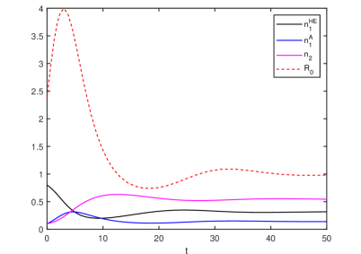
(b)

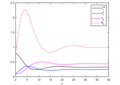
(c)

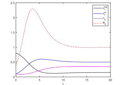
Figure 1: Time evolution of the initial data $(n_{1}^{HE},n_{1}^{A},n_{2})(t=0)=(0.8,0.1,0.1)$ and of the reproduction number $R_{0}$ with $\beta=1$, $\bar{\eta}_{11}=1$, $\bar{\eta}_{11}^{(r)}=0.1$. Panel (a): $\bar{\eta}_{21}^{(r)}=0.1$, $\bar{\mu}_{1}^{(r)}\,\hat{I}_{1}=0.3$, $\bar{\mu}_{2}^{(r)}\,\hat{I}_{2}=0.05$. Panel (b): $\bar{\eta}_{21}^{(r)}=0.4$, $\bar{\mu}_{1}^{(r)}\,\hat{I}_{1}=0.3$, $\bar{\mu}_{2}^{(r)}\,\hat{I}_{2}=0.05$. Panel (c): $\bar{\eta}_{21}^{(r)}=0.1$, $\bar{\mu}_{1}^{(r)}\,\hat{I}_{1}=0.1$, $\bar{\mu}_{2}^{(r)}\,\hat{I}_{2}=0.2$.

(a)

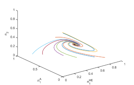
(b)

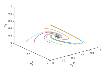
(c)

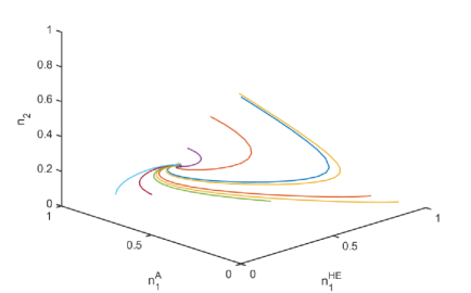
Figure 2: Phase portrait of the evolution of $n_{1}^{HE}$, $n_{1}^{A}$, $n_{2}$ for a variant with contagion rate $\beta=1$, and $\bar{\eta}_{11}=1$, $\bar{\eta}_{11}^{(r)}=0.1$. Panel (a): $\bar{\eta}_{21}^{(r)}=0.1$, $\bar{\mu}_{1}^{(r)}\,\hat{I}_{1}=0.3$, $\bar{\mu}_{2}^{(r)}\,\hat{I}_{2}=0.05$. Panel (b): $\bar{\eta}_{21}^{(r)}=0.4$, $\bar{\mu}_{1}^{(r)}\,\hat{I}_{1}=0.3$, $\bar{\mu}_{2}^{(r)}\,\hat{I}_{2}=0.05$. Panel (c): $\bar{\eta}_{21}^{(r)}=0.1$, $\bar{\mu}_{1}^{(r)}\,\hat{I}_{1}=0.1$, $\bar{\mu}_{2}^{(r)}\,\hat{I}_{2}=0.2$.

(a)

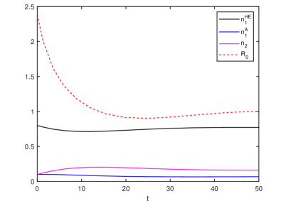
(b)

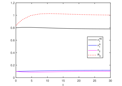
(c)

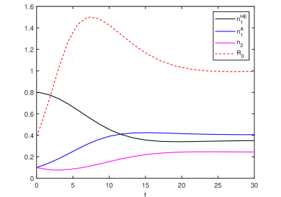
Figure 3: Time evolution of the initial data $(n_{1}^{HE},n_{1}^{A},n_{2})(t=0)=(0.8,0.1,0.1)$ and of the reproduction number $R_{0}$ with $\beta=0.7$, $\bar{\eta}_{11}=1$, $\bar{\eta}_{11}^{(r)}=0.1$. Panel (a): $\bar{\eta}_{21}^{(r)}=0.1$, $\bar{\mu}_{1}^{(r)}\,\hat{I}_{1}=0.3$, $\bar{\mu}_{2}^{(r)}\,\hat{I}_{2}=0.05$. Panel (b): $\bar{\eta}_{21}^{(r)}=0.4$, $\bar{\mu}_{1}^{(r)}\,\hat{I}_{1}=0.3$, $\bar{\mu}_{2}^{(r)}\,\hat{I}_{2}=0.05$. Panel (c): $\bar{\eta}_{21}^{(r)}=0.1$, $\bar{\mu}_{1}^{(r)}\,\hat{I}_{1}=0.1$, $\bar{\mu}_{2}^{(r)}\,\hat{I}_{2}=0.2$.

(a)

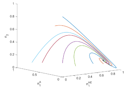
(b)

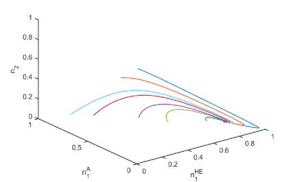
(c)

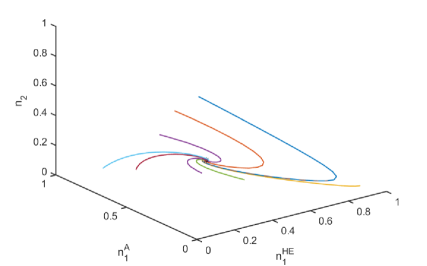
Figure 4: Phase portrait of the evolution of $n_{1}^{HE}$, $n_{1}^{A}$, $n_{2}$ for a variant with contagion rate $\beta=0.7$, and $\bar{\eta}_{11}=1$, $\bar{\eta}_{11}^{(r)}=0.1$. Panel (a): $\bar{\eta}_{21}^{(r)}=0.1$, $\bar{\mu}_{1}^{(r)}\,\hat{I}_{1}=0.3$, $\bar{\mu}_{2}^{(r)}\,\hat{I}_{2}=0.05$. Panel (b): $\bar{\eta}_{21}^{(r)}=0.4$, $\bar{\mu}_{1}^{(r)}\,\hat{I}_{1}=0.3$, $\bar{\mu}_{2}^{(r)}\,\hat{I}_{2}=0.05$. Panel (c): $\bar{\eta}_{21}^{(r)}=0.1$, $\bar{\mu}_{1}^{(r)}\,\hat{I}_{1}=0.1$, $\bar{\mu}_{2}^{(r)}\,\hat{I}_{2}=0.2$.

8 Conclusion

In this work, we have exploited the Statistical Mechanics methods in order to model the human-to-human mechanisms of SARS-CoV-2 transmission. Starting from a description of the interactions between individuals based on the Boltzmann equation (microscopic scale), we have derived a set of evolution equations for the size and mean state of each population considered, that is healthy people, positive asymptomatic, positive symptomatic and hospitalized persons (macroscopic scale). Unlike the epidemiological models that have been developed within the kinetic theory framework in the last few years, our approach does not rely on one of the existing compartmental models, but we derive a new system of macroscopic evolution equations, which aims to account for the characteristics of Covid-19. In particular, our model focuses on the role of positive-asymptomatic individuals in triggering the spread of SARS-CoV-2 virus. Asymptomatic transmission has been considered as the ”Achilles’ heel” of Covid-19 control strategies. Indeed, several studies have demonstrated that asymptomatic carriers have infected a similar number of people as symptomatic individuals [4], [24]. Beyond a trivial equilibrium solution corresponding to $n_{1}^{A}=n_{2}^{S}=n_{2}^{HS}=0$ (that is, the eradication of the disease), our model predicts, under suitable conditions on infection parameters, the existence of an endemic equilibrium which is always asymptotically stable.

Changing the value of some relevant parameters in the derived set of macroscopic equations, the following aspects of the SARS-CoV-2 spread can be addressed:

(i) The impact of the contagiousness of new variants. By setting $\beta=1$, in the stochastic law modeling the interactions between a healthy individual and a positive asymptomatic, an extremely contagious disease is described, while lower values of $\beta$ account for less infectious scenarios.

(ii) The effects of government restrictions aimed at limiting the mobility of individuals. In particular, assuming a high rate of interaction between individuals without symptoms (e.g. $\overline{\eta}_{11}=1$) means that such limitations are not applied, while lower values of $\overline{\eta}_{11}$ describe lockdown situations.

(iii) The effectiveness of specific medical treatments. The key parameter in this respect is $\overline{\eta}_{21}^{(r)}$, which describes the rate of interaction between the medical staff and the infected people belonging to population $2$. If one takes increasing values of $\overline{\eta}_{21}^{(r)}$, our model equations allow to study the efficacy of new drugs in order to control the spread of the disease until its complete (possibly) eradication.

(iv) The role of the innate and adaptive immunity in setting the severity of Covid-19. The peculiarity of SARS-CoV-2 infection is traced back to a complex interplay between the virus and the immune system. It involves pathogenic cell activation leading to hyperinflammation with a major complication of the disease. This aspect can be taken into account in the macroscopic equations we derived by choosing large values of the term ($\overline{\mu}_{1}^{(r)}\,\hat{I}_{1}$), which models the average action of the innate immune system on asymptomatic individuals (who have already contracted the virus). Furthermore, relying on clinical data, our model provides for the possibility that ill persons recover without specific treatments, by assuming large values of the term ($\overline{\mu}_{2}^{(r)}\,\hat{I}_{2}$), which describes the overall response of the adaptive immune system on individuals belonging to population $2$. Since adaptive immunity can be acquired through the administration of vaccines, which in turn increase the anti-viral activity of some innate immune cells, our system of equations allows one also to assess the impact of vaccination by increasing the term ($\overline{\mu}_{2}^{(r)}\,\hat{I}_{2}$) and, at the same time, decreasing ($\overline{\mu}_{1}^{(r)}\,\hat{I}_{1}$).

The numerical test cases presented in Section 7 highlight the ability of our model to reproduce qualitatively the salient features of Covid-19, as experienced in very recent years. Future research should be aimed at a quantitative comparison of the mathematical results with the medical data collected during the recent pandemic, in order to organize also these data in a more systematic way.

Appendix A: Equivalent formulations of the Boltzmann collision operator

In the kinetic theory of gases, based on an evolution equation of the distribution function $f(t,\mathbf{x},\mathbf{v})$ (depending on time $t\in\mathbb{R}_{+}$, space $\mathbf{x}\in\mathbb{R}^{3}$, molecular velocity $\mathbf{v}\in\mathbb{R}^{3}$), different collision–like operators have been proposed in the literature, in order to describe the effects due to binary interactions between gas particles. Specifically, for a single monatomic gas, one can prove the equivalence of the following formulations of the Boltzmann collision operator [3]. Analogous results hold also for mixtures of different monatomic constituents [21].

(a) Kinetic formulation:

$$Q(f,f)(\mathbf{v})=\int_{\mathbb{R}^{3}}d\mathbf{w}\int_{\mathbb{S}^{2}}g\,I(g,\chi)\,[f(\mathbf{v^{\prime}})f(\mathbf{w^{\prime}})-f(\mathbf{v})f(\mathbf{w})]\,d\hat{\Omega}^{\prime}.$$ (A.1)

In the classical form, the Boltzmann collision term is a quadratic operator provided by the difference between a gain and a loss contribution [5]. In the gain term, distributions are depending on pre-collision velocities $\mathbf{v^{\prime}},\mathbf{w^{\prime}}$ corresponding to the post-collision ones $\mathbf{v},\mathbf{w}$. The relative velocity of the interacting particles is denoted by

$$\mathbf{g}=\mathbf{v}-\mathbf{w}=g\,\hat{\Omega}$$

where

$$g=|\mathbf{v}-\mathbf{w}|,\qquad\quad\hat{\Omega}=\frac{(\mathbf{v}-\mathbf{w})}{g}\,.$$

In the kernel of the integral operator (A.1) there appears the so-called differential scattering cross section $I(g,\chi)$, which depends on the relative speed and on the deflection angle of the relative motion

$$\chi=\arccos(\hat{\Omega}\cdot\hat{\Omega}^{\prime}),$$

In addition, the explicit form of the cross section is determined by the intermolecular interaction potential of the considered gaseous medium. For instance, inverse-power intermolecular potentials $V(d)=d^{-p}$ (where $d$ denotes the intermolecular distance and $p>1$) give: $I(g,\chi)=g^{-4/p}\tilde{I}(\chi)$, so that in the particular case $p=4$ (Maxwell molecules) the collision kernel ($g\,I(g,\chi)$) is independent of $g$.

If the collisions between molecules are elastic, namely momentum and kinetic energy are conserved in each collision, then the center of mass velocity is preserved

$$\mathbf{G}=\frac{1}{2}(\mathbf{v}+\mathbf{w})=\frac{1}{2}(\mathbf{v^{\prime}}+\mathbf{w^{\prime}}),$$

as well as the relative speed

$$g=|\mathbf{v}-\mathbf{w}|=|\mathbf{v^{\prime}}-\mathbf{w^{\prime}}|\,.$$

Consequently, the collision process is reversible, and pre- and post–collision velocities, corresponding to the pair $\mathbf{v},\mathbf{w}$, coincide. The relation between pre- and post-collision variables reads as

$$\left\{\begin{array}[]{rl}\mathbf{v^{\prime}}=\mathbf{G}+\frac{1}{2}g\,\hat{\Omega}^{\prime}\\ \mathbf{w^{\prime}}=\mathbf{G}-\frac{1}{2}g\,\hat{\Omega}^{\prime}\end{array}\right.$$ (A.2)

In other words, post-collision velocities are uniquely determined in terms of the pre-collision ones, once the direction of the post-collision relative velocity is given.

(b) Waldmann formulation:

$$Q(f,f)(\mathbf{v})=\int_{\mathbb{R}^{3}}\int_{\mathbb{R}^{3}}\int_{\mathbb{R}^{3}}W(\mathbf{v}^{\prime},\mathbf{w}^{\prime};\mathbf{v},\mathbf{w})[f(\mathbf{v^{\prime}})f(\mathbf{w^{\prime}})-f(\mathbf{v})f(\mathbf{w})]\,d\mathbf{w}d\mathbf{v}^{\prime}d\mathbf{w}^{\prime}.$$ (A.3)

In this probabilistic formulation, proposed in [23], the kernel $W(\mathbf{v}^{\prime},\mathbf{w}^{\prime};\mathbf{v},\mathbf{w})$ represents the microscopic probability distribution for the collision process $(\mathbf{v},\mathbf{w})\rightarrow(\mathbf{v}^{\prime},\mathbf{w}^{\prime})$. Notice that in (A.3) the integrals range over all possible values of the ingoing velocity of the partner molecule $\mathbf{w}$ and of the output velocity pair $\mathbf{v}^{\prime},\mathbf{w}^{\prime}$. For elastic collisions one has

$$W(\mathbf{v}^{\prime},\mathbf{w}^{\prime};\mathbf{v},\mathbf{w})=\frac{\displaystyle 1}{\displaystyle g}\,I(g,\chi)\,\delta(\mathbf{G}-\mathbf{G^{\prime}})\,\delta(g-g^{\prime})\,,$$ (A.4)

hence, the Waldmann kernel $W$ is symmetric with respect to changes of the order of particles $\mathbf{v}\leftrightarrow\mathbf{w}$ or of pre- and post-collision velocities $(\mathbf{v},\mathbf{w})\leftrightarrow(\mathbf{v}^{\prime},\mathbf{w}^{\prime})$.

(c) Scattering kernel formulation:

$$Q(f,f)(\mathbf{v})=\int_{\mathbb{R}^{3}}\int_{\mathbb{R}^{3}}\eta(\mathbf{v^{\prime}},\mathbf{w^{\prime}})\,A(\mathbf{v^{\prime}},\mathbf{w^{\prime}};\mathbf{v})\,f(\mathbf{v^{\prime}})f(\mathbf{w^{\prime}})\,d\mathbf{v^{\prime}}\,d\mathbf{w^{\prime}}-f(\mathbf{v})\int_{\mathbb{R}^{3}}\eta(\mathbf{v},\mathbf{w})\,f(\mathbf{w})\,d\mathbf{w}.$$ (A.5)

An analogous probabilistic formulation involves the scattering collision frequency defined as

$$\eta(\mathbf{v},\mathbf{w})=:\int_{\mathbb{R}^{3}}\int_{\mathbb{R}^{3}}W(\mathbf{v}^{\prime},\mathbf{w}^{\prime};\mathbf{v},\mathbf{w})\,d\mathbf{v^{\prime}}\,d\mathbf{w^{\prime}}=\int_{\mathbb{R}^{3}}\int_{\mathbb{R}^{3}}\frac{\displaystyle 1}{\displaystyle g}\,I(g,\chi)\,\delta(\mathbf{G}-\mathbf{G^{\prime}})\,\delta(g-g^{\prime})\,d\mathbf{v^{\prime}}\,d\mathbf{w^{\prime}}$$ (A.6)

and

$$\eta(\mathbf{v^{\prime}},\mathbf{w^{\prime}})\,A(\mathbf{v^{\prime}},\mathbf{w^{\prime}};\mathbf{v})=:\int_{\mathbb{R}^{3}}W(\mathbf{v}^{\prime},\mathbf{w}^{\prime};\mathbf{v},\mathbf{w})\,d\mathbf{w}=\int_{\mathbb{R}^{3}}\frac{\displaystyle 1}{\displaystyle g}\,I(g,\chi)\,\delta(\mathbf{G}-\mathbf{G^{\prime}})\,\delta(g-g^{\prime})\,d\mathbf{w}.$$ (A.7)

It can be easily checked that the transition probability $A(\mathbf{v^{\prime}},\mathbf{w^{\prime}};\mathbf{v})$ satisfies the properties

$$A(\mathbf{v^{\prime}},\mathbf{w^{\prime}};\mathbf{v})=A(\mathbf{w^{\prime}},\mathbf{v^{\prime}};\mathbf{v})\,,$$ (A.8)

$$\int_{\mathbb{R}^{3}}A(\mathbf{v^{\prime}},\mathbf{w^{\prime}};\mathbf{v})\,d\mathbf{v}=1\,.$$ (A.9)

For Maxwell molecules one has $I(g,\chi)\propto\theta(\chi)/g$, hence $\eta(\mathbf{v},\mathbf{w})=\eta$ (constant) and

$$A(\mathbf{v^{\prime}},\mathbf{w^{\prime}};\mathbf{v})\propto\frac{\theta(\chi^{*})}{g^{\prime}}\,\delta(v^{2}-(\mathbf{v^{\prime}}+\mathbf{w^{\prime}})\cdot\mathbf{v}+\mathbf{v^{\prime}}\cdot\mathbf{w^{\prime}})$$ (A.10)

where

$$\cos(\chi^{*})=\frac{2\mathbf{v}\cdot(\mathbf{v^{\prime}}-\mathbf{w^{\prime}})-v^{\prime 2}+w^{\prime 2}}{|\mathbf{v^{\prime}}-\mathbf{w^{\prime}}|^{2}}.$$

Further details on these computations are available in [3], [21], where it is also proven the equivalence between formulations (a), (b), (c) for elastic (deterministic) collisions.

The scattering kernel formalism remains valid also with stochastic collisions, occurring for instance in social or economic problems, as in simple market economies or in epidemic models. For stochastic interactions, in which $A(\mathbf{v^{\prime}},\mathbf{w^{\prime}};\mathbf{v})$ satisfies only the relationships (A.8) and (A.9), with $\mathbf{v^{\prime}},\mathbf{w^{\prime}},\mathbf{v}$ independent variables, one cannot expect conservation of momentum and energy. In the literature of kinetic equations for socio-economic sciences, it is shown the equivalence between the collision-like Boltzmann equation and Markovian jump-processes, described by transition probabilities related to the Waldmann formulation of the Boltzmann equation [16].

Appendix B: Boltzmann operators for a reacting gas mixture

In this appendix, we present the classical reactive Boltzmann operators, originally proposed in [10, 19]. Let us consider a mixture of four gas species which, besides all elastic collisions, can interact according to the following reversible bimolecular reaction:

$$1+2\rightleftarrows 3+4.$$ (B.1)

Let us also introduce the symbols $m_{i}$ and $E_{i}$, which stand for particle mass and internal energy of chemical bond of $i$th-species ($i=1,\dots,4$), respectively. Notice that the conservation of mass implies the following constraint: $m_{1}+m_{2}=m_{3}+m_{4}=:M$.

We assume that the internal energies $E_{i}$ are such that

$$\Delta E=E_{3}+E_{4}-E_{1}-E_{2}\geq 0\,.$$ (B.2)

Consequently, the direct reaction $1+2\rightarrow 3+4$ is endothermic, thus providing an increase of chemical energy and a decrease of kinetic energy (total energy, i.e. kinetic plus internal, is preserved); on the other hand, the reverse reaction $3+4\rightarrow 1+2$ is exothermic, giving a decrease of the internal energy.

In such reactive frame, the Boltzmann equation for the distribution $f_{i}$ reads as

$$\frac{\partial f_{i}}{\partial t}(t,\mathbf{v})=\sum_{j=1}^{4}Q^{ij}+\overline{Q}^{i}\;\;\;\;\;\;\;i=1,\ldots,4,$$ (B.3)

where $Q^{ij}$ is the elastic binary operator for collisions involving a pair of species $(i,j)$, while $\overline{Q}^{i}$ is the chemical collision operator, describing the effects on species $i$ due to the reaction (B.1). When a pair of particles $(i,j)$, with molecular velocities $(\mathbf{v},\mathbf{w})$, collides, yielding a pair of molecules $(h,k)$ with velocities $\mathbf{v^{\prime}}$ and $\mathbf{w^{\prime}}$, respectively, the differential scattering cross section in the collision kernel is labeled by $I_{ij}^{hk}$. In elastic collisions one has $(h,k)=(i,j)$, while in the chemical operator $(i,j,h,k)\in\{(1,2,3,4),(2,1,4,3),(3,4,1,2),(4,3,2,1)\}$.

In Eq. (B.3), the elastic operator $Q^{ij}$ reads as

$$Q^{ij}=\int_{\mathbb{R}^{3}}d\mathbf{w}\int_{\mathbb{S}^{2}}g\,I_{ij}^{ij}(g,\hat{\Omega}\cdot\hat{\Omega}^{\prime})\,[f_{i}(\mathbf{v^{\prime}})\,f_{j}(\mathbf{w^{\prime}})-f_{i}(\mathbf{v})\,f_{j}(\mathbf{w})]\,d\hat{\Omega}^{\prime}$$ (B.4)

where, taking into account momentum and energy conservation, the post-collision velocities can be written as

$$\left\{\begin{array}[]{rl}\mathbf{v^{\prime}}=\frac{\displaystyle[m_{i}\mathbf{v}+m_{j}\mathbf{w}+m_{j}g\hat{\Omega}^{\prime}]}{\displaystyle(m_{i}+m_{j})}\\ \mathbf{w^{\prime}}=\frac{\displaystyle[m_{i}\mathbf{v}+m_{j}\mathbf{w}-m_{i}g\hat{\Omega}^{\prime}]}{\displaystyle(m_{i}+m_{j})}\end{array}\right.$$ (B.5)

Chemical operators $\overline{Q}^{i}$ involve also a suitable Heaviside function $H$, which accounts for the fact that the endothermic reaction cannot occur if the kinetic energy of the ingoing molecules is not enough, namely if the relative speed does not overcome a threshold (activation energy) depending on the internal energy gap $\Delta\!E$ and on the reduced masses

$$\mu_{ij}=\frac{\displaystyle m_{i}m_{j}}{\displaystyle(m_{i}+m_{j})}\,.$$

If the following microreversibility of reactions is invoked, which relates the cross section of the direct reaction to that of the reverse one:

$$\big{(}\mu_{12}\big{)}^{2}g^{2}\,I_{12}^{34}(g,\hat{\Omega}\cdot\hat{\Omega}^{\prime})=\big{(}\mu_{34}\big{)}^{2}(g^{\prime})^{2}\,I_{34}^{12}(g^{\prime},\hat{\Omega}\cdot\hat{\Omega}^{\prime})\qquad\text{for}\qquad g^{2}>\frac{\displaystyle 2\Delta E}{\displaystyle\mu_{12}}\,,$$ (B.6)

then, the chemical collision term in Eq. (B.3) for species $1$ is given by

$$\overline{Q}^{1}=\int_{\mathbb{R}^{3}}\int_{\mathbb{S}^{2}}H(g^{2}-\frac{\displaystyle 2\Delta E}{\displaystyle\mu_{12}})\,g\,I_{12}^{34}(g,\hat{\Omega}\cdot\hat{\Omega}^{\prime})\bigg{[}\bigg{(}\frac{\displaystyle\mu_{12}}{\displaystyle\mu_{34}}\bigg{)}^{3}\,f_{3}(\mathbf{v^{\prime}})f_{4}(\mathbf{w^{\prime}})-f_{1}(\mathbf{v})f_{2}(\mathbf{w})\bigg{]}\,d\mathbf{w}\,d\hat{\Omega}^{\prime}$$ (B.7)

where post-collision velocities take the form

$$\left\{\begin{array}[]{rl}\mathbf{v^{\prime}}=\frac{1}{M}\Big{(}m_{1}\mathbf{v}+m_{2}\mathbf{w}+m_{4}\,g^{\prime}\,\hat{\Omega}^{\prime}\Big{)}\\ \mathbf{w^{\prime}}=\frac{1}{M}\Big{(}m_{1}\mathbf{v}+m_{2}\mathbf{w}-m_{3}\,g^{\prime}\,\hat{\Omega}^{\prime}\Big{)}\end{array}\right.\qquad\text{with}\qquad g^{\prime}=\left[\frac{\mu_{12}}{\mu_{34}}\left(g^{2}-\frac{2\,\Delta\!E}{\mu_{12}}\right)\right]^{1/2}$$ (B.8)

For species $3$, the computation can be carried out in exactly the same way, with the only important difference that the reverse exothermic reaction (causing a loss term for species $3$) may occur for any relative speed of the colliding particles; thus, in the kernel there is no need of a Heaviside function, and the operator turns out to be

$$\overline{Q}^{3}=\int_{\mathbb{R}^{3}}\int_{\mathbb{S}^{2}}g\,I_{34}^{12}(g,\hat{\Omega}\cdot\hat{\Omega}^{\prime})\bigg{[}\bigg{(}\frac{\displaystyle\mu_{34}}{\displaystyle\mu_{12}}\bigg{)}^{3}\,f_{1}(\mathbf{v^{\prime}})f_{2}(\mathbf{w^{\prime}})-f_{3}(\mathbf{v})f_{4}(\mathbf{w})\bigg{]}\,d\mathbf{w}\,d\hat{\Omega}^{\prime}$$ (B.9)

where now post-collision velocities are given by

$$\left\{\begin{array}[]{rl}\mathbf{v^{\prime}}=\frac{1}{M}\Big{(}m_{3}\mathbf{v}+m_{4}\mathbf{w}+m_{2}\,g^{\prime}\,\hat{\Omega}^{\prime}\Big{)}\\ \mathbf{w^{\prime}}=\frac{1}{M}\Big{(}m_{3}\mathbf{v}+m_{4}\mathbf{w}-m_{1}\,g^{\prime}\,\hat{\Omega}^{\prime}\Big{)}\end{array}\right.\qquad\text{with}\qquad g^{\prime}=\left[\frac{\mu_{34}}{\mu_{12}}\left(g^{2}+\frac{2\,\Delta\!E}{\mu_{34}}\right)\right]^{1/2}$$ (B.10)

The collision terms for species $2$ and $4$ are analogously calculated by suitable permutations of indices in $\overline{Q}^{1}$ and $\overline{Q}^{3}$, respectively.

Concerning Maxwell molecules, if for the direct reaction we assume a constant value of

$$\nu_{12}^{34}=\int_{\mathbb{S}^{2}}I_{12}^{34}(g,\hat{\Omega}\cdot\hat{\Omega}^{\prime})d\hat{\Omega}^{\prime}\,,$$

then, taking into account microreversibility (B.6), for the cross section of the reverse reaction one gets

$$\int_{\mathbb{S}^{2}}I_{34}^{12}(g,\hat{\Omega}\cdot\hat{\Omega}^{\prime})d\hat{\Omega}^{\prime}=\left(\frac{\mu_{12}}{\mu_{34}}\right)^{3/2}\left(1+\frac{2\Delta\!E}{\mu_{34}\,g^{2}}\right)\nu_{12}^{34}\,.$$

Declarations

Data Availability

Tha data that support the findings of this study are available from the corresponding author.

Conflict of interest

The authors declare that they have no conflict of interests.

References

- [1] Albi, G., Bertaglia, G., Boscheri, W., Dimarco, G., Pareschi, L., Toscani, G., Zanella, M.: Kinetic modelling of epidemic dynamics: Social contacts, control with uncertain data, and multiscale spatial dynamics. In: Bellomo, N., Chaplain, M. A. J. (eds.) Predicting pandemics in a globally connected world, Vol. 1, pp. 43–108, Birkhäuser (2022)
- [2] Bernoulli, D.: Essai d’une nouvelle analyse de la mortalité causée par la petite vérole. Mém. Math. Phys. Acad. Roy. Sci., Paris, 1–45, In Histoire de l’Academie Royale des Sciences (1766)
- [3] Boffi, V.C., Protopopescu, V., Spiga, G.: On the equivalence between the probabilistic, kinetic, and scattering kernel formulations of the Boltzmann equation. Physica A 164: 400–410 (1990)
- [4] Boyton, R.J., Altmann, D.M.: The immunology of asymptomatic SARS-CoV-2 infection: What are the key questions? Nature Reviews Immunology 21: 762–768 (2021)
- [5] Cercignani, C.: The Boltzmann Equation and its Applications. Springer, New York (1988)
- [6] Delitala, M.: Generalized kinetic theory approach to modeling spread and evolution of epidemics. Mathematical and Computer Modelling 39, 1–12 (2004)
- [7] De Lillo, S., Delitala, M., Salvatori, M.C: Modelling epidemics and virus mutations by methods of the mathematical kinetic theory for active particles. Mathematical Models and Methods in Applied Sciences 19, 1405–1425 (2009)
- [8] Della Marca, R., Loy, N., Tosin, A.: A SIR-like kinetic model tracking individuals’ viral load. Networks and Heterogeneous Media 17, 467–494 (2022)
- [9] Dimarco, G., Toscani, G.: Kinetic modeling of alcohol consumption. J. Stat. Phys. 177, 1022–1042 (2019)
- [10] Giovangigli, V.: Multicomponent Flow Modeling. Series on Modeling and Simulation in Science, Engineering and Technology, Birkhäuser, Boston (1999)
- [11] Hethcote, H. W.: The mathematics of infectious diseases. SIAM Rew. 42, 599–653 (2000)
- [12] Kermack, W.O, McKendrick, A.G.: Contributions to the mathematical theory of epidemics. Proc. R. Soc. London, Ser. A 115, 700–721 (1927)
- [13] Kermack, W.O, McKendrick, A.G.: Contributions to the mathematical theory of epidemics. II.-The problem of endemicity. Proc. R. Soc. London, Ser. A 138, 55–83 (1932)
- [14] Kermack, W.O, McKendrick, A.G.: Contributions to the mathematical theory of epidemics.III.-Further studies of the problem of endemicity. Proc. R. Soc. London, Ser. A 141, 94–122 (1933)
- [15] Lambert, J.H.: Die Tödlichkeit der Kinderblattern. Beyträge zum Gebrauche der Mathematik und deren Anwendung. Buchhandlung der Realschule, Vol. 3, Berlin, Germany (1772)
- [16] Loy, N., Tosin, A.: Markov jump processes and collision–like models in the kinetic description of multi–agent systems. Commun. Math. Sci. 18, 1539–1568 (2020)
- [17] Pareschi, L., Toscani, G.: Interacting Multiagent Systems: Kinetic equations and Monte Carlo methods. Oxford University Press, Oxford (2013)
- [18] Ross, R.: The Prevention of Malaria. John Murray, London (1911)
- [19] Rossani, A., Spiga, G.: A note on the kinetic theory of chemically reacting gases. Physica A 272, 563–573 (1999)
- [20] Siettos, C.I., Russo, L.: Mathematical modeling of infectious disease dynamics. Virulence 4, 295–306 (2013)
- [21] Spiga, G., Nonnenmacher, T., Boffi, V.C.: Moment equations for the diffusion of the particles of a mixture via the scattering kernel formulation of the nonlinear Boltzmann equation. Physica A 131, 431–448 (1985)
- [22] Toscani, G.: Statistical description of human addiction phenomena. In: Nota, A., Albi, G., Merino-Aceituno, S., Zanella, M. (eds.) Trails in Kinetic Theory: foundational aspects and numerical methods. Springer, Berlin (2020)
- [23] Waldmann, L.: Transporterscheinungen in gasen von mittlerem druck. In: Flügge, S. (ed.), Handbuch der Physik, vol. 12. Springer Verlag, Berlin, pp. 295–514 (1958).
- [24] Wilmes, P., Zimmer, J., Schulz, J., Glod, F., Veiber, L., Mombaerts, L., Rodrigues, B., Aalto, A., Pastore, J., Snoeck, C.J., Ollert, M., Fagherazzi, G., Mossong, J., Goncalves, J., Skupin, A., Nehrbass, U.: SARS-CoV-2 transmission risk from asymptomatic carriers: Results from a mass screening programme in Luxembourg. The Lancet Regional Health-Europe 4, 100056–9 (2021)
- [25] Zhang, S. X., Marioli, F. A., Gao, R., Wang, S.: A second wave? What do people mean by Covid waves? A working definition of epidemic waves. Risk Management and Healthcare Policy 14, 3775–3782 (2021)
- [26] Zhang, X., Su, T., Jiang, D.: Dynamics of a stochastic SVEIR epidemic model incorporating general incidence rate and Ornstein-Uhlenbeck process. Journal of Nonlinear Science 33: 76 (2023)
- [27] Zhang, X.-B., Zheng, L.: Complex dynamics of a stochastic SIR epidemic model with vertical transmission and varying total population size. Journal of Nonlinear Science 33: 108 (2023)
- [28] Zhu, Q., Xu, Y., Wang, T., Xie, F.: Innate and adaptive immune response in SARS-CoV-2 infection–Current perspectives. Front. Immunol. 13, 1053437–15 (2022)