Loss induced collective mode in one-dimensional Bose gases

Abstract

We show that two-body losses induce a collective excitation in a harmonically trapped one-dimensional Bose gas, even in the absence of a quench in the trap or any other external perturbation. Focusing on the dissipatively fermionized regime, we perform an exact mode expansion of the rapidity distribution function and characterize the emergence of the collective motion. We find clear coherent oscillations in both the potential and kinetic energies as well as in the phase space quadrupole mode of the gas. We also discuss how this loss induced collective mode differs from the well known breathing mode studied in the absence of dissipation.

Introduction:

Collective modes in harmonically trapped atomic gasses are long-lived excitations involving the coherent motion of the system as a whole. The dynamics of such excitations contain important information about the quantum correlations, nature of the interactions, and symmetries of a many-body system. This class of modes has been the subject of extensive theoretical studies and many such excitations have been observed experimentally [1].

This physics is usually studied in settings where the particle number and energy are conserved quantities, that is when the system’s dynamics are ruled by the unitary time evolution. In order to excite these modes, it is necessary to abruptly change the harmonic trapping potential or induce some other small density perturbation. Similarly, the sudden coupling to an environment of any form will leave the system in a non-equilibrium state. It is an open question whether the subsequent redistribution of particles, momenta, and energy following a loss event can result in long-lived collective oscillations [2] of harmonically trapped gases.

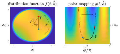
Figure 1: Typical snapshot of the rapidity distribution function at time $\tilde{t}>0$ in phase space for both planar position-momentum $\tilde{x}-\tilde{k}$ (left panel) and polar energy-angle $\tilde{e}-\tilde{\phi}$ (right panel) coordinates. The harmonic confinement induces a rotation at a frequency $\omega$ (solid arrow), while losses that involve pairs of particles (blue and red dots) at the same position (black solid line) and different momenta occur at a rate $\Gamma$. Starting from an isotropic distribution function, the losses produce periodic anisotropies that oscillate at a frequency $2\omega$ as highlighted by polar coordinates. These can be detected in the moments of the distribution function.

In this Letter we study a loss induced collective mode (LICM) in a paradigmatic example of an open quantum system: the Lieb-Liniger model of one-dimensional (1D) interacting bosons with two-body losses [3, 4, 5, 6, 7, 8, 9, 10, 11, 12, 13]. Such losses can be readily achieved in experiment using photoassociation [7] or inelastic two-body scattering [14]. In the limit of strong two-body losses or strong local interactions there is a dissipative fermionization of the gas [5, 3, 4, 10, 11, 12, 13]; states with multiple bosons at a given position are quickly removed after several loss events, while fermionized (hard-core) bosonic states become weakly dissipative. The consequences of these fermionic correlations on the number of particles has been examined both in free-space [3, 4, 10] and in harmonic traps, [11, 15, 16]. Using a lossy Boltzmann equation for the density distribution and performing its exact mode expansion in phase space, we identify and characterize signatures of the LICM in the oscillations of the potential and kinetic energies at exactly twice the harmonic trap frequency. Our analysis shows that this collective mode at leading order is a quadrupolar oscillation in phase space. Remarkably, such mechanism is uniquely enabled by losses and persists up to all times accessible with our numerics.

The Boltzmann Equation and Dynamics of the Moments:

Consider the Lieb-Liniger model of interacting bosons with two-body losses. For strong interactions the system can be described in terms of fermionic modes, rapidities, with momentum $k$ [4]. These modes are weakly dissipative with an effective two-body loss rate: $\Gamma=2\gamma/(g^{2}+\gamma^{2}/4)$ [11] that depends on both the two-body elastic, $g$, and inelastic, $\gamma$, collision strengths of the bosons .

Starting from a Lindblad master equation the dynamics of these fermionic modes can be captured using a time-dependent generalized Gibbs ensemble [10, 11], or via a derivative expansion of the quantum kinetic equation in the Keldysh theory [15, 16, 18], both of which result in an effective Boltzmann equation :

$$\left[\partial_{t}+k\partial_{x}-\omega^{2}x\partial_{k}\right]f_{k}(x,t)=-\Gamma\int_{q}(k-q)^{2}f_{q}(x,t)f_{k}(x,t).$$ (1)

In Eq. (1) we define $f_{k}(x,t)$ (with $x$ and $t$ being the position and the time, respectively) as the local distribution of fermionic rapidities with momentum $k$, and $\omega$ as the trap frequency. We also define the shorthand: $\int_{q}=\int dq/(2\pi)$ and $\int_{x}=\int dx$. For simplicity we will work with the units:

$$\tilde{x} =\frac{x}{R}, \tilde{k} =\frac{ka^{2}}{R}, \tilde{\Gamma} =\Gamma\left(\frac{R}{a}\right)^{3}, \tilde{t} =\omega t,$$ (2)

where $a=1/\sqrt{\omega}$ is the harmonic oscillator length, and $R=\sqrt{2\mu/\omega^{2}}$ is the Thomas-Fermi radius. The above units differ from Ref. [11] as we define $\tilde{t}$ in terms of $\omega$ to highlight the oscillatory physics.

We initialize the distribution of the rapidites at zero-temperature: $f_{\tilde{k}}(\tilde{x},0)=\theta(1-\tilde{k}^{2}-\tilde{x}^{2})$. A schematic of the distribution function at time $\tilde{t}$ is shown in the left panel of Fig. (1). At finite times the distribution function is no longer isotropic due to the two-body losses, which are local in $\tilde{x}$ but not in $\tilde{k}$. As we will discuss below, this anisotropy is important in the dynamics of the LICM.

In terms of observables, the decay of the total number of particles $N(t)/N(0)=2\int_{\tilde{x},\tilde{k}}f_{\tilde{k}}(\tilde{x},\tilde{t})$ was studied in [11, 15]. Moreover, it is also possible to examine other moments of the rapidity distribution, $\langle O(\tilde{x},\tilde{k})\rangle(\tilde{t})=\int_{\tilde{x},\tilde{k}}O(\tilde{x},\tilde{k})f_{\tilde{k}}(\tilde{x},\tilde{t})$ for some observable $O(\tilde{x},\tilde{k})$.

In particular, consider the size (squared) of the gas in position and momentum space, $\langle\tilde{x}^{2}\rangle(t)$ and $\langle\tilde{k}^{2}\rangle(t)$, respectively, which correspond to the potential and kinetic energies of the gas. The dynamics of these two observables are shown in Fig. (2) and exhibit two main features. The first is that there is an envelope that decays as $\tilde{t}^{-1}$ at long times. Given that these are extensive quantities, their decay is equivalent to the decrease in the overall number of particles [11, 15]. The second feature is that there are persistent oscillations at exactly twice the trap frequency, $2\omega$. The amplitude of these oscillations decreases with decreasing $\tilde{\Gamma}/\omega$. In other words, if $\tilde{\Gamma}/\omega\to 0$, the system remains in thermal equilibrium and there are no oscillations. In any case, these oscillations are the hallmark of the collective mode, and this shows that the gas begins to exhibit collective dynamics after particle loss.

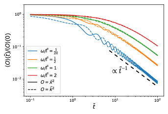
Figure 2: Results for the potential (kinetic) energy $O=\tilde{x}^{2}$ ($O=\tilde{k}^{2}$) from numerically evaluating Eq. (1) for various $\omega/\tilde{\Gamma}$. Different colors indicate different values of the ratio $\omega/\tilde{\Gamma}$ while the potential and kinetic energies are denoted by the solid and dashed lines, respectively. The scaling behaviour of $\tilde{t}^{-1}$ is shown by the black dashed line.

In order to gain insight on these oscillations we perform a phase space mode expansion of the Boltzmann equation. Instead of working with position and momentum, we work with modified polar coordinates $\tilde{e}=\tilde{x}^{2}+\tilde{k}^{2}$ and $\tilde{\phi}=\arctan(\tilde{k}/\tilde{x})$, as shown in the right panel of Fig. (1). After transforming to the new basis $f_{\tilde{k}}(\tilde{x},\tilde{t})\rightarrow g(\tilde{e},\tilde{\phi},\tilde{t})$, we expand the distribution function in terms of angular harmonics in phase space:

$$g(\tilde{e},\tilde{\phi},\tilde{t}) = g_{0}(\tilde{e},\tilde{t})$$

$$+ \sum_{m\neq 0}^{\infty}g_{m}(\tilde{e},\tilde{t})\cos(2m\tilde{\phi})+g_{-m}(\tilde{e},\tilde{t})\sin(2m\tilde{\phi}).$$

Here we consider only even harmonics as the Boltzmann equation is invariant under parity ($\tilde{k}\to-\tilde{k}$ and $\tilde{x}\to-\tilde{x}$), and our initial conditions are even under parity. In terms of these harmonics the Boltzmann equation has a simple form:

$$\partial_{\tilde{t}}g_{m}(\tilde{e},\tilde{t})+2mg_{-m}(\tilde{e},\tilde{t})=-\frac{\tilde{\Gamma}}{\omega}\mathcal{A}_{m}\left[g(\tilde{e},\tilde{\phi},\tilde{t})\right],$$ (4)

with the initial condition: $g(\tilde{e},\tilde{\phi},0)=g_{0}(\tilde{e},0)=\theta(1-\tilde{e})$. The left hand side of Eq. (4) states that modes with different $|m|$ are decoupled and that they oscillate at a frequency $2|m|\omega$. The coupling between modes with different $|m|$ is due to the two-body losses and is contained in the function $\mathcal{A}_{m}[g(\tilde{e},\tilde{\phi},\tilde{t})]$ . This function depends on the specific mode $m$, and the full distribution function $g(\tilde{e},\tilde{\phi},t)$. The explicit form of this function is shown in the supplementary materials (SM) [20].

The mode expansion in Eq. (4) is exact. However, by redefining the time of each differential equation as $\tilde{t}\rightarrow 2|m|\tilde{t}$ we observe that the loss-induced coupling to higher modes goes as $1/|m|$. Thus it is reasonable to truncate the expansion at small $|m|$ and for small $\tilde{\Gamma}/\omega$. To this end consider Fig. (3), where we examine the amplitude of the $|m|$th mode: $G_{m}(\tilde{e},\tilde{t})=\left(g_{m}^{2}(\tilde{e},\tilde{t})+g_{-m}^{2}(\tilde{e},\tilde{t})\right)^{1/2}$ for various values $\omega/\tilde{\Gamma}$. One can immediately see that for fixed $\omega/\tilde{\Gamma}$, higher harmonics are indeed suppressed (a), while each mode with $m\neq 0$ is also suppressed as $\omega/\tilde{\Gamma}\to\infty$ (b). Hence the numerical analysis shows that the mode expansion can effectively be truncated at $|m|=1$ for large $\omega/\tilde{\Gamma}$ . In fact, it is evident that there is a sizeable $g_{\pm 1}(\tilde{e},\tilde{t})$ in Fig. (1), whereas other periodicities in $\phi$ are indiscernible.

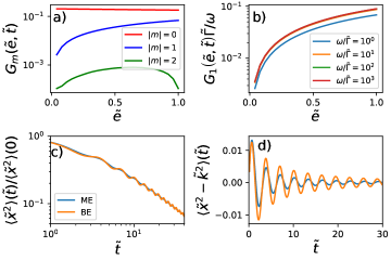
Figure 3: Amplitude of the $m$th mode $G_{m}(\tilde{e},\tilde{t})=\left(g_{m}^{2}(\tilde{e},\tilde{t})+g_{-m}^{2}(\tilde{e},\tilde{t})\right)^{1/2}$ at $\tilde{t}=\tilde{\Gamma}/\omega$ for a) fixed $\omega/\tilde{\Gamma}=1$ and various $|m|$, and b) for fixed $|m|=1$ and various $\omega/\tilde{\Gamma}$. a) Modes with higher $m$ are suppressed at fixed $\omega/\tilde{\Gamma}$. b) In the limit of large $\omega/\tilde{\Gamma}$ and fixed $|m|$, $G_{m}(\tilde{e},\tilde{t})$ vanishes as $\omega/\tilde{\Gamma}$. This is evident from the data collapse upon rescaling $G_{m}(\tilde{e},\tilde{t})$. We compare the results for c) the potential energy and d) the phase space quadrupole mode calculated using the mode expansion (ME) and the Boltzmann equation (BE).

The mode expansion is also beneficial from the point of view of calculating and understanding the dynamics of observables, as they also depend on a finite number of modes:

$$N(\tilde{t}) =\int_{0}^{\infty}d\tilde{e}\ g_{0}(\tilde{e},\tilde{t}),\quad E(\tilde{t})=\int_{0}^{\infty}d\tilde{e}\tilde{e}g_{0}(\tilde{e},\tilde{t}),$$

$$\langle\tilde{x}^{2}\rangle(\tilde{t}) =\int_{0}^{\infty}d\tilde{e}\frac{\tilde{e}}{2}\left(g_{0}(\tilde{e},\tilde{t})+\frac{1}{2}g_{1}(\tilde{e},\tilde{t})\right),$$

$$\langle\tilde{k}^{2}\rangle(\tilde{t}) =\int_{0}^{\infty}d\tilde{e}\frac{\tilde{e}}{2}\left(g_{0}(\tilde{e},\tilde{t})-\frac{1}{2}g_{1}(\tilde{e},\tilde{t})\right),$$ (5)

where we also defined the total energy of the gas $E(\tilde{t})$. Upon examining Eqs. (4-18), one can immediately see that the the function $g_{0}(\tilde{e},\tilde{t})$ is responsible for the dynamics of the number of particles and the overall decay of the potential and kinetic energies as $\tilde{t}^{-1}$, while the oscillations are due to the dynamics of $g_{1}(\tilde{e},\tilde{t})$. To isolate the oscillations, it is necessary to consider an observable that only depends on $g_{1}(\tilde{e},\tilde{t})$, such as the phase space quadrupole mode :

$$\langle\tilde{x}^{2}-\tilde{k}^{2}\rangle(\tilde{t})=\int_{0}^{\infty}de\frac{e}{2}g_{1}(e,\tilde{t}).$$ (6)

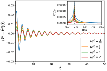
Figure 4: Phase space quadrupole mode, Eq. (6) vs $\tilde{t}$ for various values of $\omega/\tilde{\Gamma}$. The phase space quadrupole mode only depends on $g_{1}(e,t)$ and as such does not contain the envelope $\propto\tilde{t}^{-1}$. The oscillations appear to be at a single frequency, $2\omega$. The inset shows a fast Fourier transform of this data as a function of frequency $\Omega$. For each $\omega/\tilde{\Gamma}$ the Fourier transform reveals a single frequency $\Omega=2\omega$, given by the black vertical dashed line.

The dynamics of this phase space quadrupole mode as calculated from Eq. (1) are shown in Fig. (4). This quantity oscillates at a single frequency $2\omega$ as evident from the structure of the Fourier transform in the inset. Although this frequency appears independent of $\omega/\tilde{\Gamma}$, we note this is due to the truncation of the expansion at the leading order of the dissipative dynamics [15, 11] performed to obtain Eq. (1). We expect that the frequency of the oscillations will change as a function of the interaction $\Gamma$ if one includes finite elastic collisions between the fermionic modes scaling as $g/(g^{2}+\gamma^{2})$ [23].

The initial amplitude of these oscillations depends on $\tilde{\Gamma}/\omega$, and becomes vanishingly small as $\tilde{\Gamma}/\omega\to 0$, as expected. After a period of initial growth, the phase space quadrupole then undergoes damping. However, in the long-time limit there appears to be residual undamped oscillations present.

We further corroborate the validity of the mode expansion by comparing the dynamics of the potential energy $\langle\tilde{x}^{2}\rangle$ and the phase space quadrupole mode $\langle\tilde{x}^{2}-\tilde{k}^{2}\rangle$ calculated from the full Boltzmann equation, Eq. (1), and the mode expansion, Eq. (4), truncated at $|m|=1$ in Fig. (3) (c) and (d). Both approaches qualitatively agree with one another; the mode expansion is accurate at capturing the overall decay of the potential energy and the frequency of the oscillations. However, there appears a discrepancy in the decay of the phase space quadrupole mode. This discrepancy systematically decreases as the ratio $\omega/\tilde{\Gamma}$ is increased, showing that the physics can be accurately captured by the truncated mode epxansion.

Dynamics of the density profile:

We next consider the dynamics of the density during these oscillations. In Fig. (5) we present the results for the density at various times $\tilde{t}$ normalized to the instantaneous number of particles $N(\tilde{t})$. The top panel shows the density at short times, where each time corresponds to either a maximum (solid lines), or a minimum (dashed lines) of the oscillations in $\langle\tilde{x}^{2}\rangle(\tilde{t})$. Similarly, the bottom panel corresponds to later times. For short times, the density profile at a maximum (of $\langle\tilde{x}^{2}\rangle(\tilde{t})$) resembles the initial Thomas-Fermi distribution, while at a minimum it is more concentrated in the center and resembles a Gaussian. This is due to the fact that losses initially excite the quadrupole mode of the gas causing this asymmetry between maxima and minima. At long times the amplitude of the quadrupole mode has decreased but it is still finite. Thus the difference between the density distribution at the maxima and the minima decreases up to small residual quadrupolar oscillations.

This long-time dynamics can be captured considering small fluctuations $\delta g(\tilde{e},\tilde{\phi},\tilde{t})$ on top of a static distribution $\tilde{g}_{0}(e)$. The fluctuations have a spatial periodicity of $\cos(2\tilde{\phi})$ and oscillate a frequency $2\omega$ thus being a superposition of the $m=\pm 1$ modes only. Using the following ansatz:

$$g(\tilde{e},\tilde{\phi},\tilde{t})\approx N(\tilde{t})\left(\tilde{g}_{0}(\tilde{e})+\delta g(\tilde{e},\tilde{\phi},\tilde{t})\right)$$ (7)

in the mode expansion, one can reproduce the overall $\tilde{t}^{-1}$ behaviour of the number of particles, and that the effective two-body loss rate also vanishes as $\tilde{t}^{-1}$. This analysis support the important result that the oscillations become undamped in the long-time limit $\lim_{\tilde{t}\to\infty}G_{\pm 1}(\tilde{t})\neq 0$, consistent with the numerics in Figs. (4) and (5).

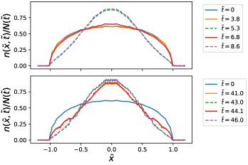
Figure 5: Dynamics of the density for short times (top panel) and long times (bottom panel). The solid lines correspond to the maxima of the oscillations of $\langle\tilde{x}^{2}\rangle(\tilde{t})$, while the dashed line correspond to the minima. At short times the maxima resemble the initial Thomas-Fermi distribution with small departures at the center, while the minima has a stronger concentration at the center of the trap. At long times, both the maximum and minimum distribution resemble one another. Similar plots exist for the rapidity distribution, but out of phase with the potential energy.

Comparison to Breathing Mode:

Such dynamics in the density ought to be contrasted to the breathing mode, which has been extensively studied in the context of 1D Bose gasses [24, 25, 26, 27] in the absence of dissipation. Provided that the system is initially prepared in an equilibrium thermal state, the motion of the density profile in this case is self similar; the density profile at each moment is related to its initial value by a time-dependent rescaling of the position: $n(x,t)=\lambda^{-1}(t)n(x/\lambda(t),0)$ for some time-dependent function $\lambda(t)$. In both the short- and long-time limits, the dynamics depicted in Fig. (5) are not self similar following a non-trivial time dependence.

We further analyze the peculiar features of the LICM by considering a second protocol; the two body losses are turned off after a hold time $t_{h}$. The details of which are shown in the SM [20]. After the losses are turned off, the gas will evolve according to the unitary closed system dynamics. One can then ask what is the difference between the breathing mode emerging with a unitary-only evolution and this protocol. In both cases the moment of inertia will exhibit undamped oscillations at a frequency $2\omega$, as is required by the non-relativistic conformal symmetry [28, 29, 30, 31]. However in the latter case, the dynamics of the densities is not self-similar at all times. For $t<t_{h}$ we obtain density profiles as in Fig. (5). For $t>t_{h}$, the density distributions are again not self-similar due to the non-equilibrium nature of the quantum state generated by the lossy dynamics. Finally, for the sake of completeness, we also address a third protocol where the trap is quenched in the presence of two body losses [20]. In this case we also find that the system oscillates at a frequency of $2\omega$ with the damping controlled by the two-body loss rate.

Conclusions:

In this Letter we have found a collective mode specific to lossy 1D hardcore Bose gasses. This mode can be excited even in the absence of external perturbations and displays coherent oscillations in different physical observables at twice the harmonic confinement frequency. Typical signatures can be seen in the behaviour of the moment of inertia as well as the phase space quadrupole mode. Such quantities are easy to access experimentally by comparing the dynamics of the width of the gas in position and and momentum space.

The mechanism enabling such oscillation appears to be quite general and we expect this physics to also occur for general $k$-body losses with $k>2$ [32, 33, 34]. Such losses would lead to different mode couplings, $\mathcal{A}_{m}$, in Eq. (4), but we expect the frequency of the oscillations is still $2\omega$.

This work shows that the environment is a tool for probing quantum systems. As collective modes have played a fundamental role in characterising quantum gases, here we show that environment induced collective modes provide complementary and non-trivial information on these gasses. We leave for a future work a more detailed study of the specific properties of this environment-induced mode on the type of loss, finite elastic and inelastic collision strengths, emergent hydrodynamic behaviour and transport.

I Supplementary materials for Loss induced collective mode in one-dimensional Bose gases.

II Mode Expansion of the Boltzmann Equation

In this section we develop the mode expansion for the Boltzmann equation presented in the main text. Our starting point is the Lieb-Liniger model of interacting Bosons with two-body losses in a harmonic trap of frequency $\omega$:

$$H=\int dx\psi^{\dagger}(x) \left(-\frac{1}{2}\omega^{2}\partial_{x}^{2}\right)\psi(x)$$

$$+\frac{g}{2}\int dx\psi^{\dagger}(x)\psi^{\dagger}(x)\psi(x)\psi(x),$$ (8)

where $\psi(x)$ is a bosonic annihilation operator, $g$ is the elastic two-body interaction strength, and we have set $\hbar=m=1$. In the presence of two-body losses, the density matrix of the system evolves according the Lindblad master equation to:

$$\partial_{t}\rho(t) =-i\left[H,\rho(t)\right]$$

$$+\gamma\int dx\left[L(x)\rho(t)L^{\dagger}(x)-\frac{1}{2}\left\{L^{\dagger}(x)L(x),\rho(t)\right\}\right].$$ (9)

with $L(x)=\psi(x)\psi(x)$ is the two-body loss operator, and $\gamma$ the two-body loss rate.

In the limit of strong elastic or inelastic interactions, the system can be described in terms of fermionic modes, or rapidities, which are weakly dissipative [5, 3, 4, 10, 11, 12, 13]. As shown in Ref. [12] using the time-dependent generalized Gibbs ensemble and in Ref. [16] using the Keldysh path integral that the dynamics of these system can be described by a Boltzmann equation for the distribution of these fermionic rapidities:

$$\left[\partial_{\tilde{t}}+\left(\tilde{k}\partial_{\tilde{x}}-\tilde{x}\partial_{\tilde{k}}\right)\right] f_{\tilde{k}}(\tilde{x},\tilde{t})=$$

$$-\frac{\tilde{\Gamma}}{\omega}\int_{\tilde{q},\tilde{k}}(\tilde{k}-\tilde{q})^{2}f_{\tilde{k}}(\tilde{x},\tilde{t})f_{\tilde{q}}(\tilde{x},\tilde{t})$$ (10)

where we have defined $\int_{\tilde{x}}=\int d\tilde{x}$, $\int_{\tilde{k}}=\int d\tilde{k}/2\pi$. In terms of the bare parameters of the Lieb-Liniger model, the effective two-body loss rate is $\Gamma=2\gamma/(g^{2}+\gamma^{2}/4)$ [12]. We also use the dimensionless parameters:

$$\tilde{x} =\frac{x}{R} \tilde{k} =\frac{ka^{2}}{R} \tilde{\Gamma} =\Gamma\left(\frac{R}{a}\right)^{3} \tilde{t} =t\omega$$ (11)

where $a=1/\sqrt{\omega}$ is the harmonic oscillator length, and $R=\sqrt{2\mu/\omega^{2}}$ is the Thomas-Fermi radius.

Instead of working with $\tilde{x}$ and $\tilde{k}$ we work with modified polar coordinates:

$$\tilde{e} =\tilde{x}^{2}+\tilde{k}^{2} \phi=\arctan\left(\frac{\tilde{k}}{\tilde{x}}\right).$$ (12)

In these units the distribution transforms as: $f_{\tilde{k}}(\tilde{x},\tilde{t})\rightarrow g(\tilde{e},\phi,\tilde{t})=f_{\sqrt{\tilde{e}}\sin(\phi)}(\sqrt{\tilde{e}}\cos(\phi),\tilde{t})/2$. In terms of Eq. (12) and $g(\tilde{e},\tilde{\phi},\tilde{t})$, the Jacobian for the transformation is unity, and we define: $\int_{\tilde{e}}=\int_{0}^{\infty}d\tilde{e}$ and $\int_{\tilde{\phi}}=\int_{0}^{2\pi}d\tilde{\phi}/(2\pi)$. The value of these units is that we can perform an expansion in terms of angular harmonics:

$$g(\tilde{e},\tilde{\phi},\tilde{t})=\sum_{m=0}^{\infty}\left[g_{m}(\tilde{e},\tilde{t})\cos(2m\tilde{\phi})+g_{-m}(\tilde{e},\tilde{t})\sin(2m\tilde{\phi})\right]$$

where $m$ labels the harmonics. In principle, there are also harmonics with odd angular momentum. Harmonics with even (odd) angular momentum are even (odd) under a parity transformation, and since the Boltzmann equation also respects parity, these sectors are decoupled. Our analysis will be primarily concerned with the even harmonics.

The left hand side (LHS) of the Boltzmann equation in terms of Eq. (12) can be straightforwardly evaluated by substituting Eq. (LABEL:eq:g) into Eq. (10):

$$LHS=\partial_{\tilde{t}}g_{m}(\tilde{e},\tilde{t})+2m\omega g_{-m}(\tilde{e},\tilde{t})$$ (14)

Note in order to obtain Eq. (14) we note that $\cos(2m\tilde{\phi})$ and $\sin(2m\tilde{\phi})$ are orthogonal functions, and can be used to project out $g_{m}(\tilde{e},\tilde{t})$ and $g_{-m}(\tilde{e},\tilde{t})$, respectively.

Although the expansion of the distribution function is clearest in terms of polar coordinates, it is more beneficial to work with modified coordinates $e$ and $\tilde{x}$ as the two-body loss term is local in $\tilde{x}$. In these coordinates:

$$\cos(\tilde{\phi}) =\frac{\tilde{x}}{\sqrt{\tilde{e}}} \sin(\tilde{\phi})=\frac{\sqrt{\tilde{e}-\tilde{x}^{2}}}{\sqrt{\tilde{e}}}$$ (15)

It is still possible to use the mode expansion in Eq. (LABEL:eq:g), however, one needs to take care of the Jacobian for the transformation, and the definition of $\tilde{g}(\tilde{e},\tilde{x},\tilde{t})$ as the transformation from $\tilde{\phi}\to\tilde{x}$ is not single-valued. However, we can use the fact all the harmonics are even under parity to simplify the transformation. Thus we can define:

$$\tilde{g}(\tilde{e},\tilde{x},\tilde{t}) =g(\tilde{e},\tilde{\phi},\tilde{t})+g(\tilde{e},\pi+\tilde{\phi},\tilde{t})$$

$$\int_{\tilde{\phi}} \rightarrow\int_{\tilde{x}}^{\prime}=\int_{-\sqrt{\tilde{e}}}^{\sqrt{\tilde{e}}}d\tilde{x}\frac{1}{\pi\sqrt{\tilde{e}-\tilde{x}^{2}}}, \int_{\tilde{e}} \rightarrow\int_{\tilde{e}}$$ (16)

In these modified units, the LHS of the Boltzmann equation is the same, only the measure of the integrals changes. We now evaluate the RHS of Eq. (10) using the coordinates in Eq. (15). The result is:

$$RHS =-\frac{\tilde{\Gamma}}{\omega}\mathcal{A}_{m}$$

$$\mathcal{A}_{m} =(2-\delta_{|m|,0})\int_{0}^{1}d\tilde{e}^{\prime}\int_{-min[\sqrt{\tilde{e}},\sqrt{\tilde{e}^{\prime}}]}^{min[\sqrt{\tilde{e}},\sqrt{\tilde{e}^{\prime}}]}dx$$

$$\left[\left\{\cos(2m\tilde{\phi}),\sin(2m\tilde{\phi})\right\}\right.$$

$$\left.\times\frac{1}{\pi^{2}}\left(\sqrt{\frac{\tilde{e}-\tilde{x}^{2}}{\tilde{e}^{\prime}-\tilde{x}^{2}}}+\sqrt{\frac{\tilde{e}^{\prime}-\tilde{x}^{2}}{\tilde{e}-\tilde{x}^{2}}}\right)\tilde{g}(\tilde{e},\tilde{x},\tilde{t})\tilde{g}(\tilde{e}^{\prime},\tilde{x},\tilde{t})\right]$$ (17)

where one substitutes either $\cos(2m\tilde{\phi})$ or $\sin(2m\tilde{\phi})$ in order to obtain the effect of dissipation on the $\pm m$th mode. This follows from the orthogonality of the angular modes to project the results for a given $m$.

This mode expansion is in principle exact. As discussed in the main article, the utility of this approach is in truncating the expansion at some value of $|m|$. For example, the mode expansion at $m=0$ was presented in Ref. [11]. This mode expansion extends their result to higher harmonics.

The physical observables of interest in this can also be conveniently expressed in terms of the modes $m=0,\pm 1$:

$$N(\tilde{t}) =\int_{0}^{\infty}d\tilde{e}\ g_{0}(\tilde{e},\tilde{t}),$$

$$E(\tilde{t}) =\int_{0}^{\infty}d\tilde{e}\ \tilde{e}g_{0}(\tilde{e},\tilde{t}),$$

$$\langle\tilde{x}^{2}\rangle(\tilde{t}) =\int_{0}^{\infty}d\tilde{e}\frac{\tilde{e}}{2}\left(g_{0}(\tilde{e},\tilde{t})+\frac{1}{2}g_{1}(\tilde{e},\tilde{t})\right),$$

$$\langle\tilde{k}^{2}\rangle(\tilde{t}) =\int_{0}^{\infty}d\tilde{e}\frac{\tilde{e}}{2}\left(g_{0}(\tilde{e},\tilde{t})-\frac{1}{2}g_{1}(\tilde{e},\tilde{t})\right).$$ (18)

Eq. (18) also suggest there are two observables that only depend on $g_{\pm 1}(\tilde{e},\tilde{t})$:

$$\langle\tilde{x}^{2}-\tilde{k}^{2}\rangle(\tilde{t}) =\int_{\tilde{e}}\frac{\tilde{e}}{2}g_{1}(\tilde{e},\tilde{t})$$ (19)

$$\langle\tilde{x}\tilde{k}\rangle(\tilde{t}) =\int_{\tilde{e}}\frac{\tilde{e}}{4}g_{-1}(\tilde{e},\tilde{t})$$ (20)

While Eq. (19) was discussed in the main text, here we present results for both Eq. (19-20) for $\omega/\tilde{\Gamma}=1$. This is shown in Fig. (6). The dynamcis of Eq. (20) are still periodic with a frequency of $2\omega$, but there is a $\pi/4$ phase shift with respect to Eq. (19). The asymmetry with respect to the zero-axis in Eq. (20) is due to the losses which are local in $x$.

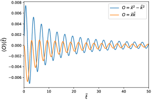
Figure 6: Comparison of the two quadrupole modes in Eqs. (19-20) for $\omega/\tilde{\Gamma}=1$ calculated according to the Boltzmann equation, Eq. (10).

III Two-Body Losses in the Non-Interacting Bose Gas

In this section we show that two-body losses can also induce oscillations in a non-interacting Bose gas. The starting point for this analysis is the Boltzmann equation:

$$\left[\partial_{t}+k\partial_{x}-\omega^{2}x\partial_{k}\right]f_{k}(x,t)=-\Gamma\int_{q}f_{q}(x,t)f_{k}(x,t).$$ (21)

In Eq. (21) $f_{k}(x,t)$ is now the local density of bosons with momentum $k$. The LHS of Eq. (21) again describes the evolution of the free bosons in a harmonic trap with frequency $\omega$, while the RHS is the two-body losses. In contrast to the case of the fermionic rapidities, bosonic statistics do not forbid a contact interaction. Thus the two-body loss term is local and does not depend on the relative momentum $(k-q)$.

In this analysis we consider all the bosons to be in their ground state:

$$f_{k}(x,0)=2N_{0}e^{-x^{2}/a^{2}-k^{2}a^{2}}$$ (22)

where $a$ is again the harmonic oscillator length, and $N_{0}$ is the initial particle number. We will work in units:

$$\tilde{x} =\frac{x}{a} \tilde{k} =ka \tilde{\Gamma} =\frac{\Gamma}{a} \tilde{t} =t\omega$$ (23)

In terms of these units the Boltzmann equation becomes:

$$\left[\partial_{\tilde{t}}+\left(\tilde{k}\partial_{\tilde{x}}-\tilde{x}\partial_{\tilde{k}}\right)\right]f_{\tilde{k}}(\tilde{x},\tilde{t})=-\frac{\tilde{\Gamma}}{\omega}\int_{\tilde{q}}f_{\tilde{q}}(\tilde{x},\tilde{t})f_{\tilde{k}}(\tilde{x},\tilde{t})$$ (24)

We will be focused on the following observables:

$$\frac{N(t)}{N_{0}} =\int_{\tilde{x},\tilde{k}}f_{\tilde{k}}(\tilde{x},\tilde{t})$$ number

$$\frac{\langle\tilde{x}^{2}\rangle(t)}{\langle\tilde{x}^{2}\rangle(0)} =\int_{\tilde{x},\tilde{k}}\tilde{x}^{2}f_{\tilde{k}}(\tilde{x},\tilde{t})$$ potential energy

$$\frac{\langle\tilde{k}^{2}\rangle(t)}{\langle\tilde{k}^{2}\rangle(0)} =\int_{\tilde{x},\tilde{k}}\tilde{k}^{2}f_{\tilde{k}}(\tilde{x},\tilde{t})$$ kinetic energy (25)

The results for the numerical simulation of Eq. (24) are shown in Fig. (7) for the number, moment of inertia, and the phase space quadrupole mode. As in the case of a nearly hardcore Bose gas, there is an overall decay of the particle number, moment of inertia, and kinetic energy. On top of this decay, the moment of inertia and kinetic energy oscillate at a frequency of $2\omega$.

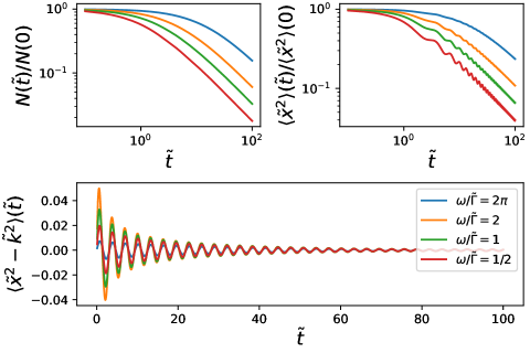
Figure 7: Dynamics of the total number (upper left), the moment of inertia (upper right), and phase space quadrupole mode (lower) for various $\omega/\tilde{\Gamma}$ for a non-interacting Bose gas with two-body losses. The behaviour of these observables is qualitatively similar to the Bose gas near the hardcore limit discussed in the main article.

This can be understood from employing the mode expansion. The only difference between the mode expansion for non-interacting bosons and hardcore bosons is the form of the right hand side of the Boltzmann equation.

IV Dynamics Following a Quench in the Harmonic Trap

We next investigate the dynamics of a strongly interacting Bose gas following a quench in the harmonic trapping potential from $\omega_{i}$ to $\omega_{f}$. Working with the units defined in Eq. (11), the Boltzmann equation is given by Eq. (10) with $\omega=\omega_{f}$. The main difference is the initial conditions. Assuming the system is initially in thermal equilibrium at zero temperature in the initial harmonic trap, the initial distribution function has the form:

$$f_{\tilde{k}}(\tilde{x},0)=\theta\left(1-\tilde{k}^{2}-\frac{\omega_{i}^{2}}{\omega_{f}^{2}}\tilde{x}^{2}\right)$$ (26)

The initial distribution function is now anisotropic. As a result, not only the $m=0$ terms in the mode expansion is initially populated, but also terms with higher $m$.

In Fig. (8) we present the results for a quench in the harmonic trap with $\omega_{i}/\omega_{f}=2$. The oscillations in $\langle x^{2}\rangle(t)$ still occur at a frequency of $2\omega_{f}$. The damping of these oscillations, unsurprisingly, depends on the strength of the dissipation. In fact, when the strength of the dissipation goes to zero, the damping rate also goes to zero.

When the two-body loss strength is zero, the system is governed by the unitary closed system dynamics. It has been well established that the dynamics of the potential energy are constrained by the non-relativistic conformal, or SO(2,1), symmetry [28, 26, 30, 31]. We have also confirmed in Fig. (8) that our numerical solution in this limit matches the prediction from conformal symmetry:

$$\frac{\langle x^{2}\rangle(t)}{\langle x^{2}\rangle(0)} =\lambda^{2}(t) \lambda^{2}(t) =\cos^{2}(\omega_{f}t)+\frac{\omega_{i}^{2}}{\omega_{f}^{2}}\sin^{2}(\omega_{f}t)$$ (27)

A key difference between the dynamics due to the quenched trap and the dynamics solely due to losses is the amplitude of the oscillations. In the absence of the quench, the amplitude of the oscillations is related to strength of the dissipation, as it is the dissipation that creates the non-equilibrium situation. In this case, after a quench, the system is initially in a highly excited non-equilibrium state. This generates oscillations with the amplitude set by the ratio $\omega_{i}/\omega_{f}$.

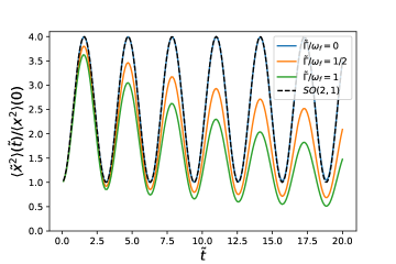
Figure 8: Dynamics of the moment of inertia, $\langle x^{2}\rangle(t)$ following a quench where $\omega_{i}/\omega_{f}=2$.

V Sudden Removal of Losses

Figure 9: Dynamics of the potential and kinetic energies. The two-body losses are finite for $0<\tilde{t}<5$, while it is zero otherwise.

Finally we consider a different experiment: a two-quench protocol in the two-body losses for a strongly interacting Bose gas. At $t=0$ we suddenly turn on the two-body losses, while at $t=t_{h}$ we suddenly remove them.

Naturally, for $0<t<t_{h}$, we expect the losses to produce oscillations in the potential and kinetic energies as discussed in the main text. For times $t>t_{h}$, these oscillations should still persist in an undamped fashion at a frequency $2\omega$ as required by the SO(2,1) symmetry of the unitary dynamics [28, 26, 29, 30, 31].

We have performed numerical simulations for such a setup, and present the results in Fig. (9) for the potential and kinetic energies, for $\omega t_{h}=5$. One can clearly see the presence of losses and the overall $t^{-1}$ decay of the potential energy in the lossy regime, $0<t<t_{h}$, and then undamped periodic oscillations for $t>t_{h}$.

Although the dynamics of the potential energy and kinetic energy are fixed by the conformal symmetry, the dynamics of the density differs from the traditional quench dynamics studied in the previous section. This is shown in Fig. (10). For the quench of the harmonic trapping potential, the dynamics of the density are self-similar, as shown from the top two panels. On the other hand, in the current experimental protocol, the dynamics of the density after the losses are turned off are not self-similar.

Theoretically this difference can be described in terms of the initial conditions, i.e. the state of the gas when the unitary closed system dynamics begin. For the case of the quench in the harmonic trapping potential, the initial state (at $t=0$) is a thermal equilibrium state within the initial harmonic trap. As discussed in Refs. [30, 31], such an initial state is diagonal in the basis of so-called conformal tower states. These conformal tower states have trivial rescaling dynamics. When the initial state is diagonal in said states, there are no intereference effects between these states, and the dynamics of observables is completely governed by the trivial time-dependent rescaling dynamics. For example the dynamics of the density are given by:

$$n(x,t)=\frac{1}{\lambda(t)}n\left(\frac{x}{\lambda(t)},0\right)$$ (28)

where $\lambda(t)$ is defined in Eq. (27).

Contrast this to the case when we suddenly remove the losses. In this case the initial state (at $t_{h}$) is in a non-equilibrium state, and is thus the state cannot be expressed as a diagonal ensemble of conformal tower states. Hence there will be non-trivial interference effects in the dynamics of the density.

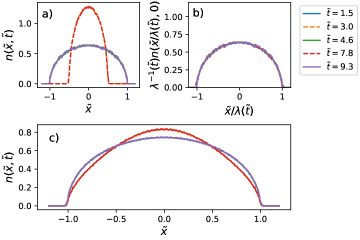
Figure 10: The dynamics of the density for a gas following a quench in the harmonic trapping potential in the absence of two-body losses (a) and b)) and following the removal of two-body losses after a hold time c). The solid (dashed) lines correspond to local maxima (minima) of the potential energy. Only for the quench in the harmonic trapping potential are rescaling dynamics of the density visible, b).

References

- Pitaevskii and Stringari [2016] L. Pitaevskii and S. Stringari, Bose-Einstein Condensation and Superfluidity, International Series of Monographs on Physics (OUP Oxford, 2016).
- Yamamoto et al. [2021] K. Yamamoto, M. Nakagawa, N. Tsuji, M. Ueda, and N. Kawakami, Collective excitations and nonequilibrium phase transition in dissipative fermionic superfluids, Phys. Rev. Lett. 127, 055301 (2021).
- Syassen et al. [2008] N. Syassen, D. M. Bauer, M. Lettner, T. Volz, D. Dietze, J. J. García-Ripoll, J. I. Cirac, G. Rempe, and S. Dürr, Strong dissipation inhibits losses and induces correlations in cold molecular gases, Science 320, 1329 (2008), https://www.science.org/doi/pdf/10.1126/science.1155309 .
- Dürr et al. [2009] S. Dürr, J. J. García-Ripoll, N. Syassen, D. M. Bauer, M. Lettner, J. I. Cirac, and G. Rempe, Lieb-liniger model of a dissipation-induced tonks-girardeau gas, Phys. Rev. A 79, 023614 (2009).
- Zhu et al. [2014] B. Zhu, B. Gadway, M. Foss-Feig, J. Schachenmayer, M. L. Wall, K. R. A. Hazzard, B. Yan, S. A. Moses, J. P. Covey, D. S. Jin, J. Ye, M. Holland, and A. M. Rey, Suppressing the loss of ultracold molecules via the continuous quantum zeno effect, Phys. Rev. Lett. 112, 070404 (2014).
- Johnson et al. [2017] A. Johnson, S. S. Szigeti, M. Schemmer, and I. Bouchoule, Long-lived nonthermal states realized by atom losses in one-dimensional quasicondensates, Phys. Rev. A 96, 013623 (2017).
- Tomita et al. [2017] T. Tomita, S. Nakajima, I. Danshita, Y. Takasu, and Y. Takahashi, Observation of the mott insulator to superfluid crossover of a driven-dissipative bose-hubbard system, Science Advances 3, e1701513 (2017), https://www.science.org/doi/pdf/10.1126/sciadv.1701513 .
- Bouchoule and Schemmer [2020] I. Bouchoule and M. Schemmer, Asymptotic temperature of a lossy condensate, SciPost Phys. 8, 060 (2020).
- Bouchoule and Dubail [2021] I. Bouchoule and J. Dubail, Breakdown of tan’s relation in lossy one-dimensional bose gases, Phys. Rev. Lett. 126, 160603 (2021).
- Rossini et al. [2021] D. Rossini, A. Ghermaoui, M. B. Aguilera, R. Vatré, R. Bouganne, J. Beugnon, F. Gerbier, and L. Mazza, Strong correlations in lossy one-dimensional quantum gases: From the quantum zeno effect to the generalized gibbs ensemble, Phys. Rev. A 103, L060201 (2021).
- Rosso et al. [2022a] L. Rosso, A. Biella, and L. Mazza, The one-dimensional Bose gas with strong two-body losses: the effect of the harmonic confinement, SciPost Phys. 12, 044 (2022a).
- Rosso et al. [2022b] L. Rosso, L. Mazza, and A. Biella, Eightfold way to dark states in su(3) cold gases with two-body losses, Phys. Rev. A 105, L051302 (2022b).
- Rosso et al. [2023] L. Rosso, A. Biella, J. De Nardis, and L. Mazza, Dynamical theory for one-dimensional fermions with strong two-body losses: Universal non-hermitian zeno physics and spin-charge separation, Phys. Rev. A 107, 013303 (2023).
- Liu et al. [2022] C. Liu, Z.-Y. Shi, and C. Wang, Weakly interacting bose gas with two-body losses (2022), arXiv:2209.10427 [cond-mat.quant-gas] .
- Gerbino et al. [2023] F. Gerbino, I. Lesanovsky, and G. Perfetto, Large-scale universality in quantum reaction-diffusion from keldysh field theory (2023), arXiv:2307.14945 .
- Perfetto et al. [2023a] G. Perfetto, F. Carollo, J. P. Garrahan, and I. Lesanovsky, Reaction-limited quantum reaction-diffusion dynamics, Phys. Rev. Lett. 130, 210402 (2023a).
- Note [1] In this definition and hereafter we set where is the particle mass.
- Huang et al. [2023] C.-H. Huang, T. Giamarchi, and M. A. Cazalilla, Modeling particle loss in open systems using keldysh path integral and second order cumulant expansion, Phys. Rev. Res. 5, 043192 (2023).
- Note [2] Our definition for differs from that in Ref. [11] by a factor of to match standard conventions.
- [20] See the supplementary materials.
- Note [3] We note that the mode expansion truncated at was reported in Ref. [11].
- Note [4] There is another quadrupole mode, , which depends solely on . The dynamics of this observable are discussed in the SM [20].
- Lenarčič et al. [2018] Z. Lenarčič, F. Lange, and A. Rosch, Perturbative approach to weakly driven many-particle systems in the presence of approximate conservation laws, Phys. Rev. B 97, 024302 (2018).
- Menotti and Stringari [2002] C. Menotti and S. Stringari, Collective oscillations of a one-dimensional trapped bose-einstein gas, Phys. Rev. A 66, 043610 (2002).
- Moritz et al. [2003] H. Moritz, T. Stöferle, M. Köhl, and T. Esslinger, Exciting collective oscillations in a trapped 1d gas, Phys. Rev. Lett. 91, 250402 (2003).
- Minguzzi and Gangardt [2005] A. Minguzzi and D. M. Gangardt, Exact coherent states of a harmonically confined tonks-girardeau gas, Phys. Rev. Lett. 94, 240404 (2005).
- Fang et al. [2014] B. Fang, G. Carleo, A. Johnson, and I. Bouchoule, Quench-induced breathing mode of one-dimensional bose gases, Phys. Rev. Lett. 113, 035301 (2014).
- Pitaevskii and Rosch [1997] L. P. Pitaevskii and A. Rosch, Breathing modes and hidden symmetry of trapped atoms in two dimensions, Phys. Rev. A 55, R853 (1997).
- Werner and Castin [2006] F. Werner and Y. Castin, Unitary gas in an isotropic harmonic trap: Symmetry properties and applications, Phys. Rev. A 74, 053604 (2006).
- Maki and Zhou [2019] J. Maki and F. Zhou, Quantum many-body conformal dynamics: Symmetries, geometry, conformal tower states, and entropy production, Phys. Rev. A 100, 023601 (2019).
- Maki and Zhou [2020] J. Maki and F. Zhou, Far-away-from-equilibrium quantum-critical conformal dynamics: Reversibility, thermalization, and hydrodynamics, Phys. Rev. A 102, 063319 (2020).
- Riggio et al. [2023] F. Riggio, L. Rosso, D. Karevski, and J. Dubail, Effects of atom losses on a one-dimensional lattice gas of hardcore bosons (2023), arXiv:2307.02298 [cond-mat.quant-gas] .
- Minganti et al. [2023] F. Minganti, V. Savona, and A. Biella, Dissipative phase transitions in -photon driven quantum nonlinear resonators, Quantum 7, 1170 (2023).
- Perfetto et al. [2023b] G. Perfetto, F. Carollo, J. P. Garrahan, and I. Lesanovsky, Quantum reaction-limited reaction-diffusion dynamics of annihilation processes, Phys. Rev. E 108, 064104 (2023b).