You Only Need One Color Space: An Efficient Network for
Low-light Image Enhancement

Abstract

Low-Light Image Enhancement (LLIE) task tends to restore the details and visual information from corrupted low-light images. Most existing methods learn the mapping function between low/normal-light images by Deep Neural Networks (DNNs) on sRGB and HSV color space. Nevertheless, enhancement involves amplifying image signals, and applying these color spaces to low-light images with a low signal-to-noise ratio can introduce sensitivity and instability into the enhancement process. Consequently, this results in the presence of color artifacts and brightness artifacts in the enhanced images. To alleviate this problem, we propose a novel trainable color space, named Horizontal/Vertical-Intensity (HVI). It not only decouples brightness and color from RGB channels to mitigate the instability during enhancement but also adapts to low-light images in different illumination ranges due to the trainable parameters. Further, we design a novel Color and Intensity Decoupling Network (CIDNet) with two branches dedicated to processing the decoupled image brightness and color in the HVI space. Within CIDNet, we introduce the Lightweight Cross-Attention (LCA) module to facilitate interaction between image structure and content information in both branches, while also suppressing noise in low-light images. Finally, we conducted 22 quantitative and qualitative experiments to show that the proposed CIDNet outperforms the state-of-the-art methods on 11 datasets. The code will be available at https://github.com/Fediory/HVI-CIDNet.

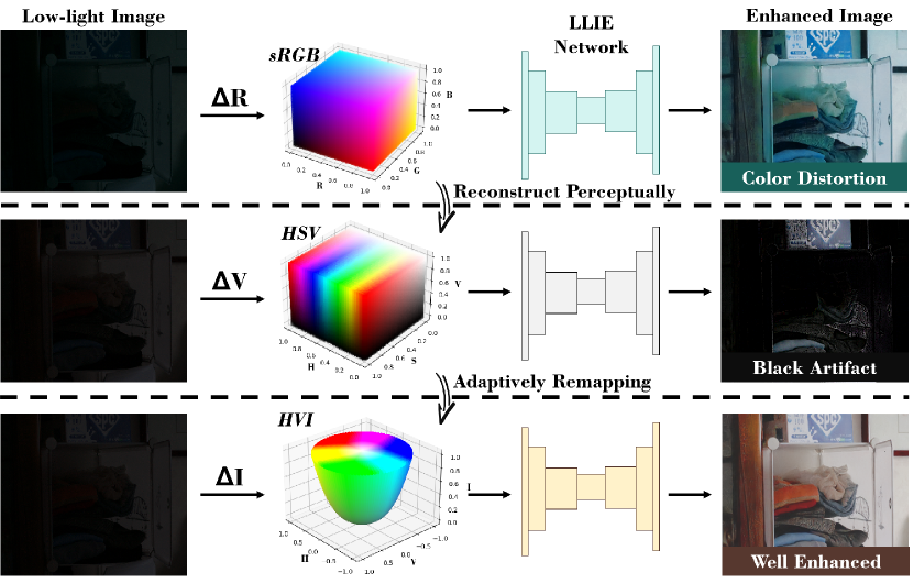
Figure 1: The sensitivity comparison of different color spaces in low-light enhancement. The notations $\Delta$R, $\Delta$V, and $\Delta$I represent a tiny variation in the axis of Red (sRGB), Value (HSV), and Intensity (HVI), respectively. After enhancement processing, noticeable color artifacts can be observed in the result in the sRGB and HSV space.

1 Introduction

Under low-light conditions, the sensor captures weak light signals with severe noise, resulting in poor visual quality for low-light images. Obtaining high-quality images often necessitates low-light image enhancement, with the goal of improving the brightness while simultaneously reducing the impact of noise and color bias Li et al. (2022).

The majority of existing approaches Zhang et al. (2019); Jiang et al. (2021); Guo et al. (2020) focus on finding an appropriate image brightness, and they commonly employ Deep Neural Networks (DNNs) to learn the mapping relationship between low-light images and normal-light images within the sRGB space. However, information such as image brightness and color exhibits a strong interdependence with the three channels in sRGB. Noise in any channel significantly impacts both the brightness and color of the image. As illustrated in Fig. 1, introducing noise to one dimension in the sRGB space dramatically alters the enhanced image’s color. This suggests a misalignment between sRGB space and the low-light enhancement processing, resulting in instability in both brightness and color in the enhanced results. It is due to this inherent instability that many enhancement methods Wang et al. (2021); Jiang et al. (2021) require more parameters and complex structures to learn this enhancement mapping. It is also the reason why numerous low-light enhancement methods Wei et al. (2018); Fu et al. (2023) need to incorporate additional brightness and color losses during training.

While the HSV color space Guo and Hu (2023) enables the separation of brightness and color of the image from RGB channels, the discontinuous nature of its Hue axis and its intricate mapping relationships with sRGB makes it challenging to handle complex and varying lighting conditions. As shown in Fig. 1, enhancing images using the HSV space can result in black artifacts due to even minor noise.

To address the aforementioned issue between the low-light image enhancement task and existing color spaces, we introduce a new color space named Horizontal/Vertical-Intensity (HVI), designed specifically to cater to the needs of low-light enhancement tasks. The proposed HVI color space not only decouples brightness and color information but also incorporates three trainable representation parameters and a trainable function, allowing it to adapt to the brightening scale and color variations of different low-light images. Building upon the HVI color space, to fully leverage the decoupled information, we propose a new LLIE method, Color and Intensity Decoupling Network (CIDNet). CIDNet consists of two pathways. After applying the HVI transformation to the image, it is separately fed into the HV-way, responsible for extracting color, and the Intensity-way, responsible for establishing the photometric mapping function under different lighting conditions. Additionally, to enhance the interaction between the structures of images contained in the brightness and color branches, we propose the bidirectional Lightweight Cross-Attention (LCA) module to connect the HV-way and Intensity-way. Furthermore, we conducted experiments and ablation studies on multiple datasets to validate our approach. The experimental results demonstrate that our method, CIDNet, not only effectively enhances the brightness of low-light images while preserving their natural colors but also exhibits relatively small parameter and computational loads. This validates the compatibility of the proposed HVI color space with low-light image enhancement tasks.

Our contributions can be summarized as follows:

1. We have introduced a HVI color space with trainable parameters, which not only decouples the image brightness and color, but also adapts to various image illumination scales.

2. Based on the HVI color space, we propose a novel Two-way network, CIDNet, to concurrently process the brightness and color of low-light images.

3. We design a bidirectional LCA to facilitate interaction between the HV-way and intensity-way, allowing the scene information in each branch to complement and improve the visual effects of the enhanced image.

4. We conducted 22 quantitative and qualitative experiments that our CIDNet outperforms all types of SOTA methods on 10 different metrics across 11 datasets.

2 Related Work

2.1 Low-Light Image Enhancement

Traditional and Plain Methods. Plain methods usually enhanced image by histogram equalization Abdullah-Al-Wadud et al. (2007) and Gama Corrction Huang et al. (2013). Traditional Methods Fu et al. (2016) commonly depend on the application of the Retinex theory, which decomposed the lights into illumination and reflections. For example, Guo et al. Guo et al. (2017) refine the initial illumination map to optimize lighting details by imposing a structure prior. Regrettably, existing methodologies are inadequate in effectively eliminating noise artifacts and producing accurate color mappings, rendering incapable of achieving the desired level of precision and finesse in LLIE task.

Deep Learning Methods. Deep learning-based approaches Lore et al. (2016); Zhang et al. (2019); Jiang et al. (2021); Cai et al. (2023) has been widely used in LLIE task. For instance, RetinexNet Wei et al. (2018) enhancing images based on Retinex theory. RUAS Risheng et al. (2021) unrolled with architecture search to construct lightweight yet effective LLIE network. SNR-Aware Xu et al. (2022) present a collectively exploiting Signal-to-Noise-Ratio-aware transformers to dynamically enhance pixels with spatial-varying operations. Still, all of these methods are recovered on sRGB space, which is not only inaccurately controlled in terms of brightness, but also biased in terms of color.

2.2 Color Space

Figure 2: The overview CIDNet pipeline of our method. (a) HVI Color Transform (HVIT): It takes an sRGB image as input and generates HV feature, Intensity feature, and HVI map as outputs. (b) CID Two-way UNet: This module performs the main processing, utilizing a Two-way UNet architecture. Lastly, we apply Perceptual-inverse HVI Transform (PHVIT), which takes a light-up HVI map as input and transforms it to an sRGB enhanced image.

RGB. Any additive color space based on RGB color model belongs to the RGB color space. Currently the most common used is the standard-RGB (sRGB) color space. For the same principle as visual recognition by the human eye, sRGB is widely used in digital imaging devices Poynton (2003). Nevertheless, sRGB is coupled in three axis and not suitable for enhancement as Section 1 presenting.

HSV and HSL. Hue, Saturation and Value or Lightness color space is a method of representing points in an RGB color model in a cylindrical coordinate system Foley and van Dam (1982). Indeed, it does decoupled brightness and color of the image from RGB channels. However, the inherent hue axis color discontinuity and non-mono-mapped pure black planes pose significant challenges when attempting to enhance the image in HSV color space, resulting in the emergence of highly pronounced artifacts.

3 HVI Color Space

To sort out the aforementioned color space challenges, we first present a trainable Horizontal/Vertical-Intensity (HVI) color space. It consists of three trainable parameters and a custom training function that can adapt to the photosensitive characteristics and color sensitivities of the dataset. Specifically, our focus lies on developing a mono-mapping transform that enables the conversion between sRGB and HVI.

3.1 Intensity Map

Any single sRGB image $\mathbf{I}\in\mathbb{R}^{\mathrm{H\times W\times 3}}$ can be decomposed into three image $\mathbf{I_{c}}\in\mathbb{R}^{\mathrm{H\times W}}$ where $\mathbf{c}\in\{R,G,B\}$ . There we denote the pixel point light intensity by

$$\mathbf{I}_{max}=\max_{\mathbf{c}\in\{R,G,B\}}(\mathbf{I_{c}})$$ (1)

which represent intensity map.

3.2 HV Color Map

We model a HV Color map as a plane to quantify color-reflectance map, which can be trained. Inspired by the weakness of the tiny value of low-lights in sRGB, we customized a parameter $k$ that allows networks to adjust the color point density of the low intensity color plane, which quantified a Color-Density-$k$ $\mathbf{C}_{k}$ as

$$\mathbf{C}_{k}=\sqrt[k]{\sin(\frac{\mathbf{I}_{max}\pi}{2})+\mathcal{\varepsilon}}$$ (2)

where $k\in\mathbb{R}$, $k>0$, and we set $\mathcal{\varepsilon}=1\times 10^{-8}$. Parameter $k$ is customizable or trainable. We formulate a bijective Color-Saturation map as

$$\mathbf{S}=\begin{cases}0,&\mathbf{I}_{max}=\mathbf{0}\\ \frac{\Delta}{\mathbf{I}_{max}},&\mathbf{I}_{max}\neq\mathbf{0}\\ \end{cases}\\$$ (3)

where $\Delta=\mathbf{I}_{max}-min(\mathbf{I}_{c})$. Next, we define a Color-Hue map as

$$\mathbf{H}=\begin{cases}0,&\text{if }\mathbf{C_{s}}=0\\ \frac{\mathbf{I_{G}}-\mathbf{I_{B}}}{\Delta}\mod{6},&\text{if }\mathbf{I}_{max}=\mathbf{I_{R}}\\ 2+\frac{\mathbf{I_{B}}-\mathbf{I_{R}}}{\Delta},&\text{if }\mathbf{I}_{max}=\mathbf{I_{G}}\\ 4+\frac{\mathbf{I_{R}}-\mathbf{I_{G}}}{\Delta},&\text{if }\mathbf{I}_{max}=\mathbf{I_{B}}\end{cases}$$ (4)

where Hue ($\mathbf{H}$) and Saturation ($\mathbf{S}$) follow HSV color space. In order to learn the sensitivity of each dataset (camera) to sRGB three-channel, we perform an adaptive linear Color-Perceptual map $\mathbf{P}_{\gamma}$ as

$$\mathbf{P}_{\gamma}=\begin{cases}\gamma_{G}\mathbf{H},&\text{if }0\leq\mathbf{H}<2\\ (\gamma_{B}-\gamma_{G})(\mathbf{H}-2)+2\gamma_{G},&\text{if }2\leq\mathbf{H}<4\\ (0.5-\gamma_{B})(\mathbf{H}-6)+1,&\text{if }4\leq\mathbf{H}<6\end{cases}$$ (5)

where $\gamma_{G}$ and $\gamma_{B}$ is customizable or trainable and $\gamma_{G},\gamma_{B}\in(0,0.5)$. We orthogonalize our color plane by set an intermediate variable $h=\cos(2\pi\mathbf{P}_{\gamma})$ and $v=\sin(2\pi\mathbf{P}_{\gamma})$ to be bijective. To enhance the functionality of our color space, we proposed a Function-Density-$T$ as

$$\mathbf{D}_{T}=T(\mathbf{P}_{\gamma})$$ (6)

where $T$ is a elemental function as $T(x)$ ($x$ represent an element in matrix), which is defined only $x\in\left[0,1\right]$ and satisfy $T(0)=T(1)$ and $T(x)\geq 0$. Function $T(x)$ is customizable or trainable. Finally, we formalize the HV plane as

$$\begin{split}\mathbf{\hat{H}}=\mathbf{C}_{k}\odot\mathbf{S}\odot\mathbf{D}_{T}\odot h\\ \mathbf{\hat{V}}=\mathbf{C}_{k}\odot\mathbf{S}\odot\mathbf{D}_{T}\odot v\end{split}$$ (7)

where $\odot$ denotes the element-wise multiplication.

3.3 Trainable HVI Map

We concatenate $\mathbf{\hat{H}}$, $\mathbf{\hat{V}}$, $\mathbf{I}_{max}$ in Eq. (1,7) to novel $\mathbf{I_{HVI}}\in\mathbb{R}^{\mathrm{H\times W\times 3}}$ map. Simultaneously, HVI map enables a one-to-one correspondence between each color point in the sRGB color space and the HVI color space, with the added advantage of ensuring reversibility of the transformation. This map can be recognized by computer perceptually. Not only solve it the problem of multi-mapping of pure black planes and intermittent color axis, but moreover, it can adapt itself to a variety of tasks by way of machine learning for more functionality.

We ponder there are still many potential application possibilities to explore in this color space. For instance, HVI with $T(x)=-4x(x-1)$ is a color space which filter the red related colors. Yet in this paper, we set $T(x)=1,\gamma_{G}=\frac{1}{6},\gamma_{B}=\frac{1}{3}$ to simplify the process and to satisfy image enhance assignment.

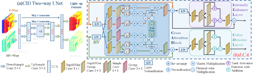
Figure 3: (a)Architrcture of CID Two-way UNet. The core module of Cross-Attention block for LLIE is (b)Lightweight Cross-Attention (LCA), which incorporate a Cross Attention Block (CAB), a Intensity Enhance Layer (IEL) and a Color Denoise Layer (CDL).

4 CIDNet

Our goal at Color and Intensity Decoupling Network (CIDNet) is to design a color feature decoupling Transformer that is lightweight and follows the HVI color space for LLIE task.

4.1 Pipeline

Given a low-light sRGB image, we first generate a intensity map $\mathbf{I_{I}}=\mathbf{I}_{max}$ using Eq.(1), and input the I-map with trainable density-$k$ into HVT to generate the HV-map using Eq.(7) as Fig. 2(a). Next, HVIT concatenate two maps to low-light HVI-map $\mathbf{I_{HVI}}$. I-map and HV-map embedded by two diffrent $\texttt{Conv}3\times 3$ layers and output the I-feature and HV-Feature with shape $H\times W\times C$.

The second step involves the utilization of two specific features as inputs to a CID 2ways-UNet as Fig.2(ii). It outputs the light-up I-feature and denoised HV-feature, both sending to a $\texttt{Conv}3\times 3$ layer in each way and concatenating together to a residual HVI map $\mathbf{R_{HVI}}$. There we add the low-light HVI map and residual HVI map as $\hat{\mathbf{I}}=\mathbf{I_{HVI}}+\mathbf{R_{HVI}}$.

Thereafter, we present the process of inverting HVI to sRGB as our PHVIT. Fisrtly, it decompose $\hat{\mathbf{I}}$ to $\mathbf{\hat{I}_{H}},\hat{\mathbf{I}}_{\mathbf{V}},\hat{\mathbf{I}}_{\mathbf{I}},$ and clip three maps in the range of $\left[-1,1\right]$. Below we get the density-k of the current iteration, and calculate $\mathbf{C_{k}}$ as Eq.2. PHVIT sets $\hat{h}$ and $\hat{v}$ as an intermediate variable as

$$\hat{h}=\frac{\mathbf{\hat{I}_{H}}}{\mathbf{D}_{T}\mathbf{C}_{k}+\mathcal{\varepsilon}},\hat{v}=\frac{\mathbf{\hat{I}_{V}}}{\mathbf{D}_{T}\mathbf{C}_{k}+\mathcal{\varepsilon}}$$ (8)

where we set $\mathcal{\varepsilon}=1\times 10^{-8}$ and $T(x)=1$ as mentioned in Sec. 3.3 follows Eq. 6. Here we have chosen to convert $\hat{h}$ and $\hat{v}$ to HSV color space to simplify steps as

$$\begin{split}\mathbf{\hat{C}_{h}}&=\arctan(\frac{C(-1,1,\hat{v})}{C(-1,1,\hat{h})})\mod 1\\ \mathbf{\hat{C}_{s}}&=\alpha_{s}\times\sqrt{C(-1,1,\hat{h})^{2}+C(-1,1,\hat{v})^{2}}\end{split}$$ (9)

where $\alpha_{s}$ is a customizing linear parameter to change image perceptually. The concatenation of $\mathbf{\hat{C}_{h}}$ (Hue), $\mathbf{\hat{C}_{s}}$ (Saturation) and $\hat{\mathbf{I}}_{\mathbf{I}}$ (Value) can be estimated as an HSV image, which can be converted to an sRGB image by the formula mentioned in Foley and van Dam (1982).

4.2 Structure

4.2.1 (a) CID Two-way UNet

The CID Two-way UNet embed six LCA modules into a network with two U-shape nets as Fig. 3(a). It contains an encoder with three DownSample $\texttt{Conv}3\times 3$ and a decoder with three UpSample $\texttt{Conv}3\times 3$. It inputs the I-way and HV-way feature with the shape $H\times W\times C$. Each DownSample reduces $H$ and $W$ by double and doubles the channels. Each UpSample doubles $H$ and $W$ and reduces the channels by double. Finally, it outputs a light-up residual I-way and HV-way feature as same as input tensor shape.

4.2.2 (b) Lightweight Cross-Attention

For the purpose of reduce the computational overhead of the Two-way UNet, we specially designed the Lightweight Cross-Attention (LCA) module which only has linear complexity and well-controlled color features based on Transformer Petit et al. (2021) as Fig. 3(b).

CAB. From the layer normalized tensors $\mathbf{Y_{I}},\mathbf{Y_{HV}}\in\mathbb{R}^{\hat{H}\times\hat{W}\times\hat{C}}$, our Cross Attention Block (CAB) first derives queries($\mathbf{Q}$) by $\mathbf{Q_{I}}=W_{s}^{Q}W_{p}^{Q}\mathbf{Y_{I}}$. Meanwhile, CAB synthesizes and splits keys($\mathbf{K}$) and values($\mathbf{V}$) by $\mathbf{K_{I}}=W_{s}^{K}W_{d}^{K}\mathbf{Y_{I}}$ and $\mathbf{V_{I}}=W_{s}^{V}W_{d}^{V}\mathbf{Y_{I}}$. $W_{d}^{(\cdot)}$ and $W_{p}^{(\cdot)}$ are depth-wise and point-wise $\texttt{Conv}1\times 1$ layers, and $W_{s}^{(\cdot)}$ is a group $\texttt{Conv}3\times 3$ layer. Subsequently, we re-arrange $\mathbf{Q},\mathbf{V}$ from $\hat{H}\times\hat{W}\times\hat{C}$ to $\hat{H}\hat{W}\times\hat{C}$ and $\mathbf{K}$ to $\hat{C}\times\hat{H}\hat{W}$ as $\hat{\mathbf{Q}},\hat{\mathbf{K}},\hat{\mathbf{V}}$ and formulate as

$$\begin{split}\mathbf{\hat{Y}_{I}}=W_{p}\hat{\mathbf{V}}\otimes\mathrm{Softmax}\left(\hat{\mathbf{Q}}\otimes\hat{\mathbf{K}}/\alpha_{H}\right)+\mathbf{Y_{I}}\end{split}$$ (10)

where $\alpha_{H}$ is the multi-head factor simlar to the multi-head SA Dosovitskiy et al. (2021) but divide the number of channels into the heads. The above layers are bias-free. HV-way is indentical to I-way with different input.

IEL and CDL. From the another layer normalized tensors $\mathbf{\hat{Y}^{\prime}_{I}},\mathbf{\hat{Y}^{\prime}_{HV}}\in\mathbb{R}^{\hat{H}\times\hat{W}\times\hat{C}}$, our Intensity Enhance Layer (IEL) and Color Denoise Layer (CDL) generate the light-up intensity and color decomposed tensors. CDL embeds the $\mathbf{\hat{Y}^{\prime}_{HV}}$ and split it to different color eigenvalues due to diverse light waves as $\mathbf{S_{HV}}=W_{s}^{S}W_{d}^{S}\mathbf{\hat{Y}^{\prime}_{HV}}$ and $\mathbf{C_{HV}}=W_{s}^{C}W_{d}^{C}\mathbf{\hat{Y}^{\prime}_{HV}}$ based on principal of optics BORN and WOLF (1980). CDL is defined as

$$\begin{split}\mathbf{\tilde{Y}_{HV}}=W_{d}(&(\tanh{(W_{s}\mathbf{S_{HV}})}+\mathbf{S_{HV}})\\ \odot&(\tanh{(W_{s}\mathbf{C_{HV}})}+\mathbf{C_{HV}}))\end{split}$$ (11)

where $\odot$ represent the element-wise multiplication. IEL has the same structure as CDL, but to reduce the training difficulty, IEL outputs the residuals as $\mathbf{\tilde{Y}_{I}}=\mathrm{IEL}(\mathbf{\hat{Y}^{\prime}_{I}})+\mathbf{\hat{Y}_{I}}$.

4.3 Loss Function

Given an output HVI map $\mathbf{\hat{I}_{HVI}}$ and a sRGB image $\mathbf{\hat{I}}$. Let $\mathbf{I}$ represent sRGB GroundTruth, which can be transformed to HVI map $\mathbf{I_{HVI}}$. We employ L1 loss $L_{1}$, edge loss $L_{e}$ Seif and Androutsos (2018) and perceptual loss $L_{p}$ Johnson et al. (2016) at sRGB and HVI space as

$$\begin{split}&\ l(\hat{x},x)=\lambda_{1}\cdot L_{1}(\hat{x},x)+\lambda_{e}\cdot L_{e}+\lambda_{p}\cdot L_{p}(\hat{x},x)\\ &\ L=\lambda_{c}\cdot l(\mathbf{\hat{I}_{HVI}},\mathbf{I_{HVI}})+l(\mathbf{\hat{I}},\mathbf{I})\\ \end{split}$$ (12)

where $\lambda_{c},\lambda_{1},\lambda_{e},\lambda_{p}$ are all the weight coefficients used to trade-off the loss function $L$ from our experiments.

5 Experiments

Methods	Complexity		LOLv1				LOLv2-Real				LOLv2-Syn
			Normal		GT Mean		Normal		GT Mean		Normal		GT Mean
	Params/M	FLOPs/G	PSNR	SSIM	PSNR	SSIM	PSNR	SSIM	PSNR	SSIM	PSNR	SSIM	PSNR	SSIM
RetinexNet Wei et al. (2018)	0.84	584.47	16.774	0.419	18.915	0.427	16.097	0.401	18.323	0.447	17.137	0.762	19.099	0.774
KinD Zhang et al. (2019)	8.02	34.99	17.650	0.775	20.860	0.802	14.740	0.641	17.544	0.669	13.290	0.578	16.259	0.591
ZeroDCE Guo et al. (2020)	0.075	4.83	14.861	0.559	21.880	0.640	16.059	0.580	19.771	0.671	17.712	0.815	21.463	0.848
3DLUT Zeng et al. (2020)	0.59	7.67	14.350	0.445	21.350	0.585	17.590	0.721	20.190	0.745	18.040	0.800	22.173	0.854
DRBN Yang et al. (2020)	5.47	48.61	16.290	0.617	19.550	0.746	20.290	0.831	-	-	23.220	0.927	-	-
MIRNet Zamir et al. (2020)	31.76	785.1	24.100	0.845	26.519	0.856	20.020	0.820	27.173	0.865	21.940	0.876	25.955	0.898
RUAS Risheng et al. (2021)	0.003	0.83	16.405	0.500	18.654	0.518	15.326	0.488	19.061	0.510	13.765	0.638	16.584	0.719
LLFlow Wang et al. (2021)	17.42	358.4	21.149	0.854	24.998	0.871	17.433	0.831	25.421	0.877	24.807	0.919	27.961	0.930
EnlightenGAN Jiang et al. (2021)	114.35	61.01	17.480	0.651	20.003	0.691	18.230	0.617	-	-	16.570	0.734	-	-
Restormer Zamir et al. (2022)	26.13	144.25	22.365	0.816	26.682	0.853	18.693	0.834	26.116	0.853	21.413	0.830	25.428	0.859
LEDNet Zhou et al. (2022)	7.07	35.92	20.627	0.823	25.470	0.846	19.938	0.827	27.814	0.870	23.709	0.914	27.367	0.928
SNR-Aware Xu et al. (2022)	4.01	26.35	24.610	0.842	26.716	0.851	21.480	0.849	27.209	0.871	24.140	0.928	27.787	0.941
PairLIE Fu et al. (2023)	0.33	20.81	19.510	0.736	23.526	0.755	19.885	0.778	24.025	0.803	-	-	-	-
LLFormer Wang et al. (2023)	24.55	22.52	23.649	0.816	25.758	0.823	20.056	0.792	26.197	0.819	24.038	0.909	28.006	0.927
RetinexFormer Cai et al. (2023)	1.53	15.85	25.153	0.846	27.140	0.850	22.794	0.840	27.694	0.856	25.670	0.930	28.992	0.939
CIDNet-wP	1.88	7.57	23.809	0.857	27.715	0.876	24.111	0.868	28.134	0.892	25.129	0.939	29.367	0.950
CIDNet-oP	1.88	7.57	23.500	0.870	28.141	0.889	23.427	0.862	27.762	0.881	25.705	0.942	29.566	0.950

Table 1: Quantitative comparisons PSNR/SSIM$\uparrow$ on LOL (v1 and v2) datasets. Normal and GT Mean represent with and without gamma-corrected by GroundTruth. The highest result is in red color while the second highest result is in cyan color. wP and oP represent to train on CIDNet with and without perceptual loss Simonyan and Zisserman (2015).

5.1 Datasets and Experiment Settings

Methods	LOLv1		LOLv2-Real		LOLv2-Syn		Complexity
	Normal	GT Mean	Normal	GT Mean	Normal	GT Mean	FLOPs/G$\downarrow$
EnlightenGAN	0.322	0.317	0.309	0.301	0.220	0.213	61.01
RetinexNet	0.474	0.470	0.543	0.519	0.255	0.247	587.47
LLFormer	0.175	0.167	0.211	0.209	0.066	0.061	22.52
LLFlow	0.119	0.117	0.176	0.158	0.067	0.063	358.4
LEDNet	0.118	0.113	0.120	0.114	0.061	0.056	35.92
RetinexFormer	0.131	0.129	0.171	0.166	0.059	0.056	15.85
CIDNet	0.086	0.079	0.108	0.101	0.045	0.040	7.57

Table 2: Quantitative comparisons LPIPS/FLOPs$\downarrow$ on LOL (v1 and v2) datasets. GT Mean represent the gamma-corrected image by GroundTruth. The best result is in red color.

We employed seven commonly-used LLIE benchmark datasets for evaluation, including LOLv1 Wei et al. (2018), LOLv2 Yang et al. (2021), DICM Lee et al. (2013), LIME Guo et al. (2017), MEF Ma et al. (2015), NPE Wang et al. (2013), and VV Vonikakis et al. (2018). We also conducted further experiments on two extreme datasets, SICE Cai et al. (2018) (containing mix and grad test sets Zheng et al. (2022)) and SID (Sony-Total-Dark) Chen et al. (2018). Since blurring is often prone to occur in low-luminosity images, in order to demonstrate the robustness of our CIDNet to multitasking, we conducted experiments on LOL-Blur Zhou et al. (2022) as well.

Sony-Total-Dark. The subset of SID dataset captured by Sony $\alpha$7S II camera is adopted for evaluation. There are 2697 short-long-exposure RAW image pairs. To make this dataset more challenging, we converted the RAW format images to sRGB images with no gamma correction, which resulted in images becoming extremely dark.

Experiment Settings. We implement our CIDNet by PyTorch. The model is trained with the Adam Kingma and Ba (2017) optimizer ($\beta_{1}$ = 0.9 and $\beta_{2}$ = 0.999) for at least 300 epochs by using a single NIVIDA 2080Ti or 3090 GPU. The learning rate is initially set to $1\times 10^{-4}$ and then steadily decreased to $1\times 10^{-7}$ by the cosine annealing scheme Loshchilov and Hutter (2017) during the training process. We randomly crop the image to 256 $\times$ 256 for patch size and set batch size less than 10 (which will be adjusted between datasets). When testing, we padded the input images to be a multiplier of $8\times 8$ using reflect padding on both sides. After inference, we cropped the padded image back to original size.

Evaluation Metrics. For the paired dataset, we adopt the Peak Signal-to-Noise Ratio (PSNR) and Structural Similarity (SSIM) Wang et al. (2004) as the distortion metrics. Unfortunately, PSNR is well-known to only partially correspond to human perception and can actually lead to algorithms with visibly lower quality in the reconstructed images. To evaluate the perceptual quality of restored images, we report Learned Perceptual Image Patch Similarity (LPIPS) Zhang et al. (2018) by using AlexNet Krizhevsky et al. (2012) for references as a perceptual metric. For the unpaired datasets, we evaluated single recovered images using BRISQUE Mittal et al. (2012) and NIQE Mittal et al. (2013) perceptually.

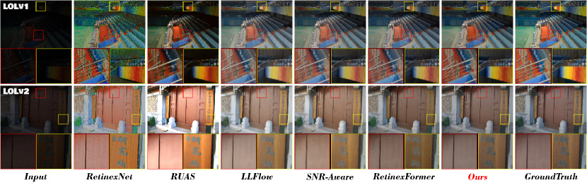
Figure 4: Visual comparisons of the enhanced results by different methods on LOLv1 and LOLv2. Zoom in for the best view.

5.2 Evaluation on Low-light Enhancement

Methods	SICE-Mix			SICE-Grad			SID-Total-Dark
	PSNR$\uparrow$	SSIM$\uparrow$	LPIPS$\downarrow$	PSNR$\uparrow$	SSIM$\uparrow$	LPIPS$\downarrow$	PSNR$\uparrow$	SSIM$\uparrow$	LPIPS$\downarrow$
RetinexNet	12.397	0.606	0.407	12.450	0.619	0.364	15.695	0.395	0.743
ZeroDCE	12.428	0.633	0.382	12.475	0.644	0.334	14.087	0.090	0.813
URetinexNet	10.903	0.600	0.402	10.894	0.610	0.356	15.519	0.323	0.599
RUAS	8.684	0.493	0.525	8.628	0.494	0.499	12.622	0.081	0.920
LLFlow	12.737	0.617	0.388	12.737	0.617	0.388	16.226	0.367	0.619
LEDNet	12.668	0.579	0.412	12.551	0.576	0.383	20.830	0.648	0.471
CIDNet	13.425	0.636	0.362	13.446	0.648	0.318	22.904	0.676	0.411

Table 3: Quantitative comparison on three hard datasets with PSNR$\uparrow$, SSIM$\uparrow$ and LPIPS$\downarrow$. The best result is in red color.

LOL Datasets Results. We quantitatively compare our CIDNet with many SOTA methods as shown in Table 1 and 2. It can be found that our method is optimal on almost all metrics for both LOLv1 and LOLv2 datasets. Despite the fact that our normal PSNR on LOLv1 dataset is lower compared to some existing methods, it should be noted that a higher PSNR method often tend to introduce more noise and result in inferior visualization. Hence, our experiment efforts are directed towards enhancing SSIM and LPIPS metrics, which are considered more effective and reliable measures for evaluating image quality.

Comparing two tables in a comprehensive manner, it can be seen that CIDNet setting six new SOTA SSIM and LPIPS results on three subsets of LOL (v1 and v2) dataset with only 7.57 GFLOPs. It outperforms the current SOTA method Retinexformer in terms of both PSNR and SSIM under GT Mean while LPIPS improves by 38%, 39%, and 29%, respectively, and FLOPs decreased by 52%. Compared to 3DLUT with about same size of FLOPs, our method significantly improves the PSNR by 6.791, 7.944, and 7.393 dB. It may be observed in Figure 4 that our model restore colors extremely well, which may be attribute to the HVI color space.

SICE and Sony-total-Dark. In order to verify that our model also performs well on large-scale datasets, we conducted experiments on two extremely difficult-to-recover datasets, SICE (including Mix and Grad) and SID-Total-Dark. The three metrics of our CIDNet are optimal on all three test sets as Table 3. especially on the SID-Total-Dark dataset, which outperforms LEDNet by 9.96% for the PSNR, 4.32% for the SSIM, 12.74% for the LPIPS metrics.

Methods	DICM		LIME		MEF		NPE		VV
	BRIS$\downarrow$	NIQE$\downarrow$	BRIS$\downarrow$	NIQE$\downarrow$	BRIS$\downarrow$	NIQE$\downarrow$	BRIS$\downarrow$	NIQE$\downarrow$	BRIS$\downarrow$	NIQE$\downarrow$
KinD	48.72	5.15	39.91	5.03	49.94	5.47	36.85	4.98	50.56	4.30
ZeroDCE	27.56	4.58	20.44	5.82	17.32	4.93	20.72	4.53	34.66	4.81
RUAS	38.75	5.21	27.59	4.26	23.68	3.83	47.85	5.53	38.37	4.29
LLFlow	26.36	4.06	27.06	4.59	30.27	4.70	28.86	4.67	31.67	4.04
SNR-Aware	37.35	4.71	39.22	5.74	31.28	4.18	26.65	4.32	78.72	9.87
PairLIE	33.31	4.03	25.23	4.58	27.53	4.06	28.27	4.18	39.13	3.57
CIDNet	21.47	3.79	16.25	4.13	13.77	3.56	18.92	3.74	30.63	3.21

Table 4: Quantitative comparison on five unpaired data sets with BRISQUE$\downarrow$ and NIQE$\downarrow$. The best result is in red color.

Unpaired Datasets Experiments. In the case of unpaired datasets DICM, LIME, MEF, NPE, and VV, where GroundTruth is unavailable, we evaluate the effectiveness of models trained on LOLv1 or LOLv2-Syn using various methods, and measure their performance using BRISQUE and NIQE metrics. We report our comparisons against SOTA methods as Table 4, where our method outperformed all previous SOTA methods. Notably, our method exhibits a substantial improvement in the NIQE metric compared to other approaches.

For each of these five unpaired datasets, we randomly selected an image in each dataset and compared visually. As Fig. 5, CIDNet improves the brightness and increases the perceived level of the image while ensuring reasonable color accuracy compared with RUAS, ZeroDCE, RetinexNet, KinD and PairLIE.

Figure 5: Five unpaired datasets were compared visually, and we randomly selected one image in each dataset to compare with the other methods. Our CIDNet is significantly better than the other methods.

gray!10Methods	gray!10 ZeroDCE $\rightarrow$ MIMO	gray!10 DeblurGAN${\dagger}$ $\rightarrow$ ZeroDCE	gray!10RetinexFormer${\ddagger}$	gray!10MIMO${\ddagger}$	gray!10LEDNet${\ddagger}$	gray!10CIDNet${\ddagger}$
PSNR$\uparrow$	17.680	18.330	22.904	24.410	25.271	26.572
SSIM$\uparrow$	0.542	0.589	0.824	0.835	0.859	0.890
LPIPS$\downarrow$	0.422	0.384	0.236	0.183	0.141	0.120
FLOPs/G$\downarrow$	-	-	15.85	62.36	35.93	7.57

Table 5: Quantitative evaluation on LOL-Blur dataset. PSNR$\uparrow$ and SSIM$\uparrow$: the higher, the better; LPIPS$\downarrow$ and FLOPs$\downarrow$: the lower, the better. The symbol ‘${\dagger}$’ indicates that we use DeblurGAN-v2 trained on RealBlur Rim et al. (2020) dataset. ‘${\ddagger}$’ indicates the network is retrained on the LOL-Blur dataset. The highest result is in red color.

5.3 Low-light Deblurring

Long exposures in dimly lit environments can result in photos that are prone to blurring. In order to verify the recovery ability of our model, we conducted experiments on the low-light blur dataset LOL-Blur.

In the first set, we perform lighting-up with ZeroDCE and then deblurring with MIMO Cho et al. (2021). In the second set, we perform deblurring with DeblurGAN-v2 Kupyn et al. (2019) and then lighting-up with ZeroDCE. In the third group, we retrained on LOL-Blur with four methods, RetinexFormer, MIMO, LEDNet, and compared them with our CIDNet. The results (as Table 5) show that the quantitative comparison of CIDNet against the current stage SOTA method LEDNet by 5.15%, 3.61%, and 14.89% in PSNR, SSIM, and LPIPS metrics respectively. Not only that, the FLOPs of our model are the smallest among these methods.

As shown in Fig. 6, we have taken a set of blurred images, recovered them using different methods, and compared them with GroundTruth. The experimental results reveal that the image reconstructions achieved by CIDNet exhibit a notable improvement in visual comfort and perceptual recognition, thereby enhancing the overall quality and interpretability of the generated images.

gray!10	gray!10Baseline	gray!10Color Space	gray!10LCA	gray!10Two-Way	gray!10CrossAttn	gray!10PSNR$\uparrow$	gray!10SSIM$\uparrow$
1	$\surd$	sRGB				16.518	0.721
2	$\surd$	sRGB	$\surd$			18.606	0.822
3	$\surd$	HSV	$\surd$			13.237	0.365
4	$\surd$	HSV	$\surd$	$\surd$		10.236	0.254
5	$\surd$	HSV	$\surd$	$\surd$	$\surd$	13.668	0.407
6	$\surd$	HVI	$\surd$			22.000	0.853
7	$\surd$	HVI	$\surd$	$\surd$		23.159	0.854
8	$\surd$	HVI	$\surd$	$\surd$	$\surd$	24.111	0.868

(a) Ablation of CIDNet module designs.

gray!10	gray!10HVI	gray!10RGB	gray!10Perceptual	gray!10PSNR$\uparrow$	gray!10SSIM$\uparrow$	gray!10LPIPS$\downarrow$
1	$\surd$			22.113	0.812	0.262
2		$\surd$		22.319	0.827	0.205
3	$\surd$	$\surd$		23.427	0.862	0.169
4	$\surd$	$\surd$	$\surd$	24.111	0.868	0.108

(b) Ablation of HVI, RGB and Perceptual losses.

Table 6: We conduct ablation study on LOLv2-Real dataset. PSNR, SSIM, LPIPS are reported. The best result is in red color.

5.4 Ablation Study

We conduct extensive ablation studies to validate proposed HVI color space and LCA module. The evaluations were performed on the LOLv2-Real dataset for fast convergence and stable performance. Results are reported in Table 6.

A. Color Spaces. We conducted an ablation on sRGB, HSV and our HVI on CIDNet as Table 6(a). The ranking of image restoration quality with CIDNet is as follows: HVI, sRGB, HSV.

B. LCA module. We further examined our proposed LCA module in present color spaces. As shown in Table 6(a) row (1), (2), (6), LCA with baseline gains 2.088, 5.428 dB on PSNR for sRGB and HVI respectively.

C. Why Two-way? In our experimental investigation, we have observed distinct statistical patterns between the I-way and HV-way. Table 6(a) row (6), (7) suggests that devide the Net in Two-way enhance 1.159 dB in PSNR.

D. Effects of Cross-Attention in LCA. By decoupling the image through HVI, a certain correlation between the values of I-map and the noise of HV-map can be discovered. To establish the relationship mapping, we incorporated Cross-Attention into the internal of LCA. As Table 6(a) row (8), PSNR and SSIM both greater than row (7) (with self-attention Zamir et al. (2022)) by 0.952 dB and 0.014.

E. Loss Ablation. We conducted an ablation by progressively adding loss on (1)HVI-map, (2)sRGB-image, (3)HVI and sRGB, (4)Perceptual-loss on both color space as Table 6(b). Compared to the previous group, LPIPS metric was a decrease of 21.8%, 17.6%, and 36.1% respectively.

F. Analysis. Experiments A to D sequentially verify the superiority of our HVI color space, LCA, Two-way UNet with Cross-Attention. For Experiment E, HVI color space needs to be supervised by the sRGB loss in order to perform. We leave deeper explorations to future works.

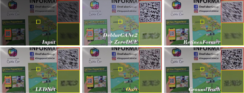
Figure 6: Visual comparision on LOL-Blur dataset. Compared to other methods, our CIDNet is closer to GroundTruth and more dominant in visual recognition. (Zoom in for best view)

6 Conclusion

In this paper, we presents a novel method for low-light image enhancement using the proposed HVI color space with trainable parameters and the CIDNet to decouple image brightness and color and adapt to various illumination scales. The Two-way network, built upon the HVI color space, simultaneously processes brightness and color, aided by the plug-and-play LCA module and symmetric HVI Transform module. Our CIDNet dramatically outperforms all types of SOTA methods across 11 datasets with lower FLOPs and parameters.

References

- Abdullah-Al-Wadud et al. [2007] M. Abdullah-Al-Wadud, Md. Hasanul Kabir, M. Ali Akber Dewan, and Oksam Chae. A dynamic histogram equalization for image contrast enhancement. In 2007 Digest of Technical Papers International Conference on Consumer Electronics, pages 1–2, 2007.
- BORN and WOLF [1980] MAX BORN and EMIL WOLF. Chapter iv - geometrical theory of optical imaging. In MAX BORN and EMIL WOLF, editors, Principles of Optics (Sixth Edition), pages 133–202. Pergamon, sixth edition edition, 1980.
- Cai et al. [2018] Jianrui Cai, Shuhang Gu, and Lei Zhang. Learning a deep single image contrast enhancer from multi-exposure images. IEEE Transactions on Image Processing, 27(4):2049–2062, 2018.
- Cai et al. [2023] Yuanhao Cai, Hao Bian, Jing Lin, Haoqian Wang, Radu Timofte, and Yulun Zhang. Retinexformer: One-stage retinex-based transformer for low-light image enhancement. In Proceedings of the IEEE/CVF International Conference on Computer Vision (ICCV), pages 12504–12513, October 2023.
- Chen et al. [2018] Chen Chen, Qifeng Chen, Jia Xu, and Vladlen Koltun. Learning to see in the dark. In CVPR, 2018.
- Cho et al. [2021] Sung-Jin Cho, Seo-Won Ji, Jun-Pyo Hong, Seung-Won Jung, and Sung-Jea Ko. Rethinking coarse-to-fine approach in single image deblurring, 2021.
- Dosovitskiy et al. [2021] Alexey Dosovitskiy, Lucas Beyer, Alexander Kolesnikov, Dirk Weissenborn, Xiaohua Zhai, Thomas Unterthiner, Mostafa Dehghani, Matthias Minderer, Georg Heigold, Sylvain Gelly, Jakob Uszkoreit, and Neil Houlsby. An image is worth 16x16 words: Transformers for image recognition at scale, 2021.
- Foley and van Dam [1982] James D. Foley and Andries van Dam. Fundamentals of interactive computer graphics. 1982.
- Fu et al. [2016] Xueyang Fu, Delu Zeng, Yue Huang, Xiao-Ping Zhang, and Xinghao Ding. A weighted variational model for simultaneous reflectance and illumination estimation. In 2016 IEEE Conference on Computer Vision and Pattern Recognition (CVPR), pages 2782–2790, 2016.
- Fu et al. [2023] Zhenqi Fu, Yan Yang, Xiaotong Tu, Yue Huang, Xinghao Ding, and Kai-Kuang Ma. Learning a simple low-light image enhancer from paired low-light instances. In Proceedings of the IEEE/CVF Conference on Computer Vision and Pattern Recognition, pages 22252–22261, 2023.
- Guo and Hu [2023] Xiaojie Guo and Qiming Hu. Low-light image enhancement via breaking down the darkness. International Journal of Computer Vision, 131(1):48–66, Jan 2023.
- Guo et al. [2017] X. Guo, Y. Li, and H. Ling. Lime: Low-light image enhancement via illumination map estimation. IEEE Transactions on Image Processing, 26(2):982–993, 2017.
- Guo et al. [2020] Chunle Guo Guo, Chongyi Li, Jichang Guo, Chen Change Loy, Junhui Hou, Sam Kwong, and Runmin Cong. Zero-reference deep curve estimation for low-light image enhancement. In Proceedings of the IEEE conference on computer vision and pattern recognition (CVPR), pages 1780–1789, June 2020.
- Huang et al. [2013] Shih-Chia Huang, Fan-Chieh Cheng, and Yi-Sheng Chiu. Efficient contrast enhancement using adaptive gamma correction with weighting distribution. IEEE Transactions on Image Processing, 22(3):1032–1041, 2013.
- Jiang et al. [2021] Yifan Jiang, Xinyu Gong, Ding Liu, Yu Cheng, Chen Fang, Xiaohui Shen, Jianchao Yang, Pan Zhou, and Zhangyang Wang. Enlightengan: Deep light enhancement without paired supervision. IEEE Transactions on Image Processing, 30:2340–2349, 2021.
- Johnson et al. [2016] Justin Johnson, Alexandre Alahi, and Li Fei-Fei. Perceptual losses for real-time style transfer and super-resolution, 2016.
- Kingma and Ba [2017] Diederik P. Kingma and Jimmy Ba. Adam: A method for stochastic optimization, 2017.
- Krizhevsky et al. [2012] Alex Krizhevsky, I. Sutskever, and G. Hinton. Imagenet classification with deep convolutional neural networks. Advances in neural information processing systems, 25(2), 2012.
- Kupyn et al. [2019] Orest Kupyn, Tetiana Martyniuk, Junru Wu, and Zhangyang Wang. Deblurgan-v2: Deblurring (orders-of-magnitude) faster and better. In The IEEE International Conference on Computer Vision (ICCV), Oct 2019.
- Lee et al. [2013] Chulwoo Lee, Chul Lee, and Chang-Su Kim. Contrast enhancement based on layered difference representation of 2d histograms. IEEE Transactions on Image Processing, 22(12):5372–5384, 2013.
- Li et al. [2022] Chongyi Li, Chunle Guo, Linghao Han, Jun Jiang, Ming-Ming Cheng, Jinwei Gu, and Chen Change Loy. Low-light image and video enhancement using deep learning: A survey. IEEE Transactions on Pattern Analysis and Machine Intelligence, 44(12):9396–9416, 2022.
- Lore et al. [2016] Kin Gwn Lore, Adedotun Akintayo, and Soumik Sarkar. Llnet: A deep autoencoder approach to natural low-light image enhancement, 2016.
- Loshchilov and Hutter [2017] Ilya Loshchilov and Frank Hutter. Sgdr: Stochastic gradient descent with warm restarts, 2017.
- Ma et al. [2015] Kede Ma, Kai Zeng, and Zhou Wang. Perceptual quality assessment for multi-exposure image fusion. IEEE Transactions on Image Processing, 24(11):3345–3356, 2015.
- Mittal et al. [2012] Anish Mittal, Anush Krishna Moorthy, and Alan Conrad Bovik. No-reference image quality assessment in the spatial domain. IEEE Transactions on Image Processing, 21(12):4695–4708, 2012.
- Mittal et al. [2013] Anish Mittal, Rajiv Soundararajan, and Alan C. Bovik. Making a “completely blind” image quality analyzer. IEEE Signal Processing Letters, 20(3):209–212, 2013.
- Petit et al. [2021] Olivier Petit, Nicolas Thome, Clément Rambour, and Luc Soler. U-net transformer: Self and cross attention for medical image segmentation, 2021.
- Poynton [2003] Charles Poynton. 18 - image digitization and reconstruction. In Charles Poynton, editor, Digital Video and HDTV, The Morgan Kaufmann Series in Computer Graphics, pages 187–194. Morgan Kaufmann, San Francisco, 2003.
- Rim et al. [2020] Jaesung Rim, Haeyun Lee, Jucheol Won, and Sunghyun Cho. Real-world blur dataset for learning and benchmarking deblurring algorithms. In Proceedings of the European Conference on Computer Vision (ECCV), 2020.
- Risheng et al. [2021] Liu Risheng, Ma Long, Zhang Jiaao, Fan Xin, and Luo Zhongxuan. Retinex-inspired unrolling with cooperative prior architecture search for low-light image enhancement. In Proceedings of the IEEE Conference on Computer Vision and Pattern Recognition, 2021.
- Seif and Androutsos [2018] George Seif and Dimitrios Androutsos. Edge-based loss function for single image super-resolution. In 2018 IEEE International Conference on Acoustics, Speech and Signal Processing (ICASSP), pages 1468–1472, 2018.
- Simonyan and Zisserman [2015] Karen Simonyan and Andrew Zisserman. Very deep convolutional networks for large-scale image recognition. In International Conference on Learning Representations, 2015.
- Vonikakis et al. [2018] Vassilios Vonikakis, Rigas Kouskouridas, and Antonios Gasteratos. On the evaluation of illumination compensation algorithms. Multimedia Tools and Applications, 77:1–21, 04 2018.
- Wang et al. [2004] Zhou Wang, A.C. Bovik, H.R. Sheikh, and E.P. Simoncelli. Image quality assessment: from error visibility to structural similarity. IEEE Transactions on Image Processing, 13(4):600–612, 2004.
- Wang et al. [2013] Shuhang Wang, Jin Zheng, Hai-Miao Hu, and Bo Li. Naturalness preserved enhancement algorithm for non-uniform illumination images. IEEE transactions on image processing : a publication of the IEEE Signal Processing Society, 22, 05 2013.
- Wang et al. [2021] Yufei Wang, Renjie Wan, Wenhan Yang, Haoliang Li, Lap-Pui Chau, and Alex C Kot. Low-light image enhancement with normalizing flow. arXiv preprint arXiv:2109.05923, 2021.
- Wang et al. [2023] Tao Wang, Kaihao Zhang, Tianrun Shen, Wenhan Luo, Bjorn Stenger, and Tong Lu. Ultra-high-definition low-light image enhancement: A benchmark and transformer-based method. In Proceedings of the AAAI Conference on Artificial Intelligence, volume 37, pages 2654–2662, 2023.
- Wei et al. [2018] Chen Wei, Wenjing Wang, Wenhan Yang, and Jiaying Liu. Deep retinex decomposition for low-light enhancement. 2018.
- Xu et al. [2022] Xiaogang Xu, Ruixing Wang, Chi-Wing Fu, and Jiaya Jia. Snr-aware low-light image enhancement. In 2022 IEEE/CVF Conference on Computer Vision and Pattern Recognition (CVPR), pages 17693–17703, 2022.
- Yang et al. [2020] Wenhan Yang, Shiqi Wang, Yuming Fang, Yue Wang, and Jiaying Liu. From fidelity to perceptual quality: A semi-supervised approach for low-light image enhancement. In IEEE/CVF Conference on Computer Vision and Pattern Recognition (CVPR), June 2020.
- Yang et al. [2021] Wenhan Yang, Wenjing Wang, Haofeng Huang, Shiqi Wang, and Jiaying Liu. Sparse gradient regularized deep retinex network for robust low-light image enhancement. volume 30, pages 2072–2086, 2021.
- Zamir et al. [2020] Syed Waqas Zamir, Aditya Arora, Salman Khan, Munawar Hayat, Fahad Shahbaz Khan, Ming-Hsuan Yang, and Ling Shao. Learning enriched features for real image restoration and enhancement. In ECCV, 2020.
- Zamir et al. [2022] Syed Waqas Zamir, Aditya Arora, Salman Khan, Munawar Hayat, Fahad Shahbaz Khan, and Ming-Hsuan Yang. Restormer: Efficient transformer for high-resolution image restoration. In CVPR, 2022.
- Zeng et al. [2020] Hui Zeng, Jianrui Cai, Lida Li, Zisheng Cao, and Lei Zhang. Learning image-adaptive 3d lookup tables for high performance photo enhancement in real-time. IEEE Transactions on Pattern Analysis and Machine Intelligence, 44(04):2058–2073, 2020.
- Zhang et al. [2018] Richard Zhang, Phillip Isola, Alexei A Efros, Eli Shechtman, and Oliver Wang. The unreasonable effectiveness of deep features as a perceptual metric. In CVPR, 2018.
- Zhang et al. [2019] Yonghua Zhang, Jiawan Zhang, and Xiaojie Guo. Kindling the darkness: A practical low-light image enhancer. In Proceedings of the 27th ACM International Conference on Multimedia, MM ’19, pages 1632–1640, New York, NY, USA, 2019. ACM.
- Zheng et al. [2022] Shen Zheng, Yiling Ma, Jinqian Pan, Changjie Lu, and Gaurav Gupta. Low-light image and video enhancement: A comprehensive survey and beyond. arXiv preprint arXiv:2212.10772, 2022.
- Zhou et al. [2022] Shangchen Zhou, Chongyi Li, and Chen Change Loy. Lednet: Joint low-light enhancement and deblurring in the dark. In ECCV, 2022.