TaE: Task-aware Expandable Representation for Long Tail Class
Incremental Learning

Abstract

Class-incremental learning (CIL) aims to train classifiers that learn new classes without forgetting old ones. Most CIL methods focus on balanced data distribution for each task, overlooking real-world long-tailed distributions. Therefore, Long-Tailed Class-Incremental Learning (LT-CIL) has been introduced, which trains on data where head classes have more samples than tail classes. Existing methods mainly focus on preserving representative samples from previous classes to combat catastrophic forgetting. Recently, dynamic network algorithms frozen old network structures and expanded new ones, achieving significant performance. However, with the introduction of the long-tail problem, merely extending task-specific parameters can lead to miscalibrated predictions, while expanding the entire model results in an explosion of memory size. To address these issues, we introduce a novel Task-aware Expandable (TaE) framework, dynamically allocating and updating task-specific trainable parameters to learn diverse representations from each incremental task, while resisting forgetting through the majority of frozen model parameters. To further encourage the class-specific feature representation, we develop a Centroid-Enhanced (CEd) method to guide the update of these task-aware parameters. This approach is designed to adaptively minimize the distances between intra-class features while simultaneously maximizing the distances between inter-class features across all seen classes. The utility of this centroid-enhanced method extends to all ”training from scratch” CIL algorithms. Extensive experiments were conducted on CIFAR-100 and ImageNet100 under different settings, which demonstrates that TaE achieves state-of-the-art performance.

1 Introduction

Class Incremental Learning (CIL) aims to establish a unified classifier across all known classes, and the most challenging problem of CIL is catastrophic forgetting [4]. Traditional CIL assumes that training data is formed by a balanced distribution. However, the distribution of real-world data is usually long-tailed [34], in which the number of head-classes samples is much more than the tail-class. Recently, Long-tailed Class-incremental learning (LT-CIL) has been proposed, Liu et al. took the lead in proposing two scenarios for LT-CIL: Ordered LT-CIL and Shuffled LT-CIL. [13]. We focus on the more challenging ”Shuffled LT-CIL” scenario in this paper. Shuffled LT-CIL Randomly shuffles the long-tail distribution before task construction as shown in Figure.2. Shuffled LT-CIL biases the model toward learning head classes while neglecting tail classes during new task training. This leads to a deficiency in the learning of the tail class features. Similarly, when retaining old knowledge, the model experiences more severe forgetting due to the blurring of tail class features. Consequently, for all CIL methods, the stability and plasticity of the tail classes are significantly compromised.

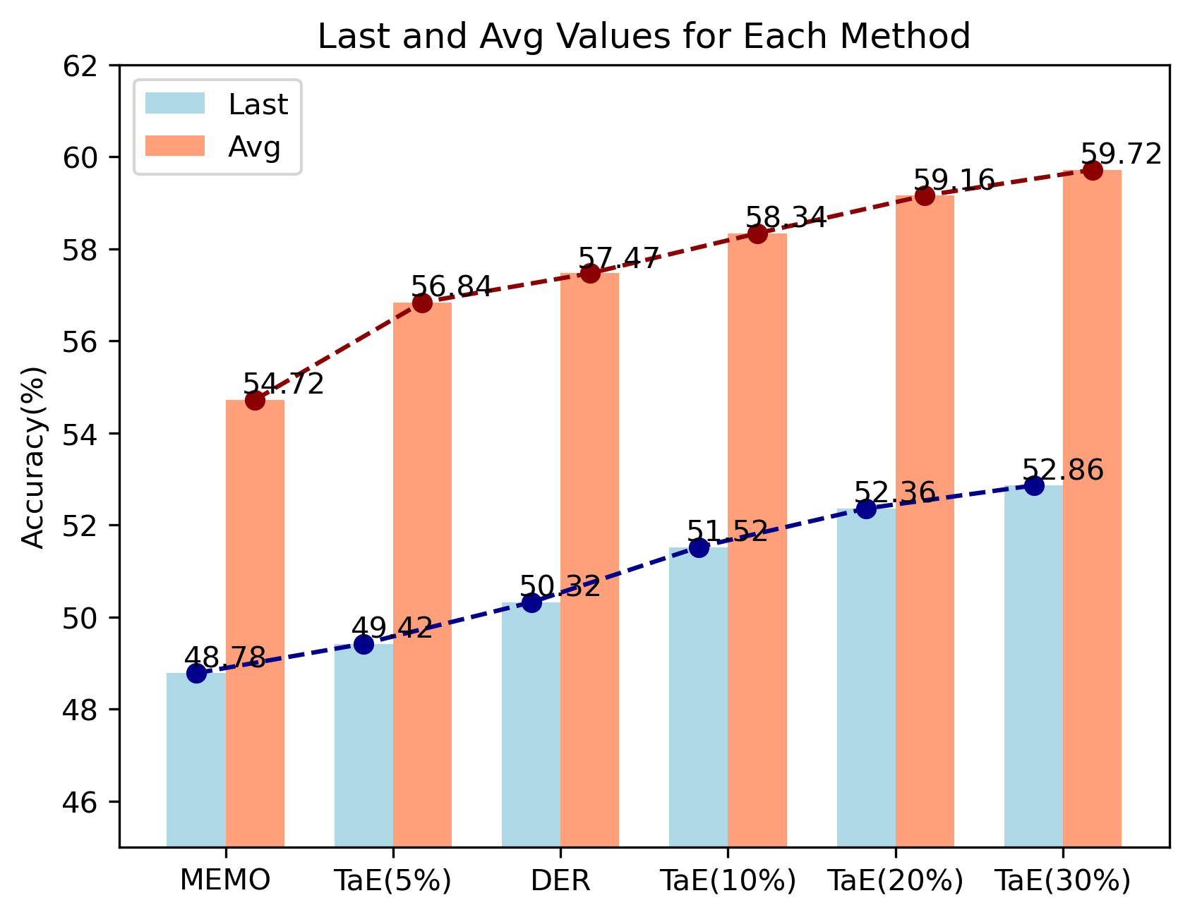
Figure 1: The Last and Average Accuracy. We compare our model($p$ = 5$\%$, 10$\%$, 20$\%$, 30$\%$) with SOTA CIL methods (DER [31] and MEMO [36]), and the model trained on the experiment Imagenet100 B0-10steps with $\rho=0.1$.

Currently, dynamic networks exhibit commendable performance in both CIL and LT-CIL [38, 31, 36, 24, 30, 13]. In LT-CIL tasks, the dynamic network’s ability to expand its structure enhances the model’s representational capacity, allowing it to better adapt to the data distribution of new tasks. As a result, the model demonstrates stronger learning capabilities in handling long-tailed distributions within new tasks. Dynamic network approaches can be roughly divided into two categories: expanding a part of the network structure, like task-specific blocks, or fully expanding the backbone. However, if shallow networks trained on the initial task are shared and frozen, and only part of the deep networks are expanded, this might lead to miscalibrated predictions due to the weak representational ability of the shallow network. Conversely, fully expanding the entire model could result in an explosion of memory size.

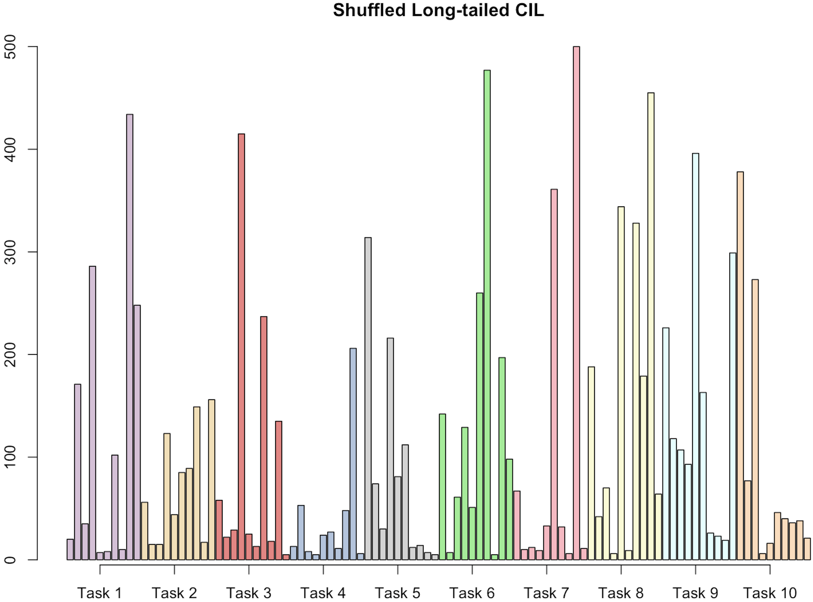
Figure 2: Shuffled LT-CIL: Task-specific long-tail distributions for Each Task

In this paper, we introduce a novel Task-aware Expandable (TaE) framework, dynamically allocating and updating task-specific trainable parameters to learn diverse representations from each incremental task, while resisting forgetting through the majority of frozen model parameters. Specifically, before training on a new task, we conduct forward propagation for each sample and accumulate the entire parameter gradients to identify the top-$p$$\%$(eg,.5$\%$, 10$\%$, 20$\%$, 30$\%$) most sensitive parameters. These parameters are then exclusively updated during training. To further enhance class-specific feature representation, we develop a Centroid-Enhanced (CEd) method to guide the update of task-aware parameters. We acquire a centroid for each class and maintain a set of centroids. These centroids are treated as learnable parameters, dynamically updated throughout the model training process to adapt to changes in the feature space resulting from the introduction of new data. This approach aims to adaptively minimize intra-class feature distances while maximizing inter-class feature distances among all observed classes. The CEd method enhances the class-specific representation of task-aware parameters, leading to an improvement in the recognition accuracy of tail classes.

We conducted experiments on two commonly used benchmark datasets, including CIFAR100 and ImageNet100. We set both datasets with a long-tail configuration and shuffled their order. We set up different degrees of long-tail and different ways of incrementation. Extensive experiments and ablation studies prove the effectiveness of our method. Especially in representative experiments on the Imagenet100 dataset, an extension by just 5$\%$ results in surpassing MEMO’s performance by 0.64$\%$ in final accuracy and 2.12$\%$ in average accuracy. Furthermore, an extension by 10$\%$ leads to surpassing DER with improvements of 1.20$\%$ and 0.87$\%$ in final accuracy and average accuracy, respectively, as depicted in Figure 1. The main contributions can be summarized in three points:

• We introduce a novel Task-aware Expandable (TaE) framework to address shuffled LT-CIL challenges, allowing adaptively parameter updates while significantly reducing the expandable model memory size.

• To further encourage the class-specific feature representation, we propose a Centroid-Enhanced (CEd) method to guide the update of these task-aware parameters and jointly address the challenge of low discriminability of tail class features in LT-CIL.

• The method we proposed achieves state-of-the-art performance on all 12 benchmarks. Notably, Our method achieves an average accuracy surpassing the SOTA by 3.69$\%$ on CIFAR-100 and 2.25$\%$ on ImageNet under the B0-10 steps with $\rho=0.1$.

2 Related Work

2.1 Class-incremental Learning

Recent CIL algorithms can be roughly divided into model-centric and algorithm-centric methods. Within the model-centric methods, dynamic network algorithms have demonstrated commendable performances. Yan et al extend a new network backbone when faced with a new task, subsequently aggregating it at the feature level with a larger classifier [31]. Wang et al contend that not all features are necessarily effective and, building on the foundation set by DER, employ knowledge distillation for model reduction [25]. Zhou et al decouples the intermediate layers of the network. Extending the deep network, reduces memory overhead, addressing the issue of excessive memory budget cost by dynamic network expansion [36]. On the other hand, within algorithm-centric methods, knowledge distillation methods stand out in terms of efficacy. Li et al were the first to employ knowledge distillation in CIL, establishing a regularization term via knowledge distillation to counteract forgetting [10]. Rebuffi et al enhances LWF by utilizing an exemplar set and introducing a novel selection method called herding [20]. However, these methods are discussed in the context of balanced data distribution. Liu et al demonstrated that their performance tends to degrade significantly in LT-CIL [13].

2.2 Long-tailed Learning

The phenomenon of long-tail data distribution is pervasive in the real world, and the challenges of long-tail learning have been studied extensively. Most existing works can be categorized into class rebalancing, information augmentation, and model improvement. Class rebalancing focuses on techniques such as resampling and reweighting. Lin et al investigated the difficulty of class prediction as a method for re-weighting [11]. Cao et al impose variable margin factors for distinct classes, determined by their training label occurrences, prompting tail classes to possess broader margins [1]. Beyond basic image manipulations such as rotation and cropping, transfer learning has also emerged as a focal point in recent research on data augmentation. Wang et al introduced a MetaNetwork that transforms few-shot model parameters to many-shot ones [27]. Liu et al focus on head-to-tail transfer at the classifier tier [12]. Yin et al leverage head-class variance insights to bolster feature augmentation for tail classes, aiming for greater intra-class variance in tail-class features [32]. In the model improvement section, the most popular research focuses on training by decoupling the feature extractor and the classifier. Kang et al first introduced the concept of a two-stage decoupled training scheme [7]. Chu et al introduced an innovative classifier re-training method using tail-class feature augmentation [2]. Although these methods perform well in class imbalance issues, applying them to sequential model training is not straightforward.

3 Method

3.1 Overview

To formalize, we consider a sequence of $B$ training tasks denoted as $\left\{{\mathcal{D}^{1},\mathcal{D}^{2},\cdots,\mathcal{D}^{B}}\right\}$, where each task $\mathcal{D}^{b}$ is characterized by $\left\{\left(\mathbf{x}_{i}^{b},{y}_{i}^{b}\right)\right\}_{i=1}^{{n}_{b}}$. Here, $\mathbf{x}_{i}^{b}\in\mathbb{R}^{D}$ represents an instance belonging to class ${y}_{i}\in{Y}_{b}$, and ${Y}_{b}$ denotes the label space of task $b$. Importantly, the label spaces for different tasks are mutually exclusive. During the training of task $t$, only data from $\mathcal{D}^{t}$ is accessible. The model’s performance is evaluated across all observed class labels, defined as $\mathcal{Y}_{b}={Y}_{1}\cup\cdots{Y}_{b}$ [38].

The Exemplar Set is an auxiliary collection of instances from previous tasks, denoted as $\mathcal{E}=\left\{\left(\mathbf{x}_{j},{y}_{j}\right)\right\}_{j=1}^{M}$, where ${y}_{j}\in\mathcal{Y}_{b-1}$. This set, combined with the current dataset, i.e., $\mathcal{E}\cup\mathcal{D}^{t}$, facilitates model updates within each task [36]. Herding, as proposed in [20], stands out as a widely adopted approach for the selection of exemplars.

The cross-entropy loss $\mathcal{L}_{ce}$ at task $t$ is define as:

$$\mathcal{L}_{ce,t}(\mathbf{x},y)=-\frac{1}{\left|\mathcal{D}^{t}\right|+\left|\mathcal{E}\right|}\sum_{(\mathbf{x},y)\in\mathcal{D}^{t}\cup\mathcal{E}}\mathbf{y}\cdot\log(p_{1:t}(\mathbf{x}))$$ (1)

where $\mathbf{y}$ is a one-hot vector in which the position of the ground-truth label is 1, and $p_{1:t}(\mathbf{x})$ is a vector with the probability predictions for image $\mathbf{x}$ overall seen classes.

For the learning of the $t$-th task, our approach involves the following three steps:
1) Extraction and Expansion of Task-aware Parameters Stage. In order to mitigate network storage explosion and extend the network structure more suitable for the current task, we first forward propagate the data of the new task through the pre-existing network for $n$ iterations. Subsequently, we accumulate and average the gradients of all parameters in the network over these iterations. This process allows us to identify the top $p$$\%$ of parameters with the most active gradient, and only these parameters can be trained.
2) Centroid-Enhanced Stage. To enhance feature distinctiveness between new and old classes, as well as among long-tail classes, we establish centroids for each seen class and update their centroids during model training. The $\mathcal{L}_{max-min}$ objective is employed to bring features of the same class closer to their respective centroids while ensuring that centroids of different classes move farther apart from each other.
3) Classifier Learning Stage. As the number of classes increases, we regenerate and train classifiers. Due to the data imbalance among long-tail classes and the imbalance between exemplar sets and current task data, we employ a Re-weight strategy to address these disparities. An overview of our approach is illustrated in Figure 3.

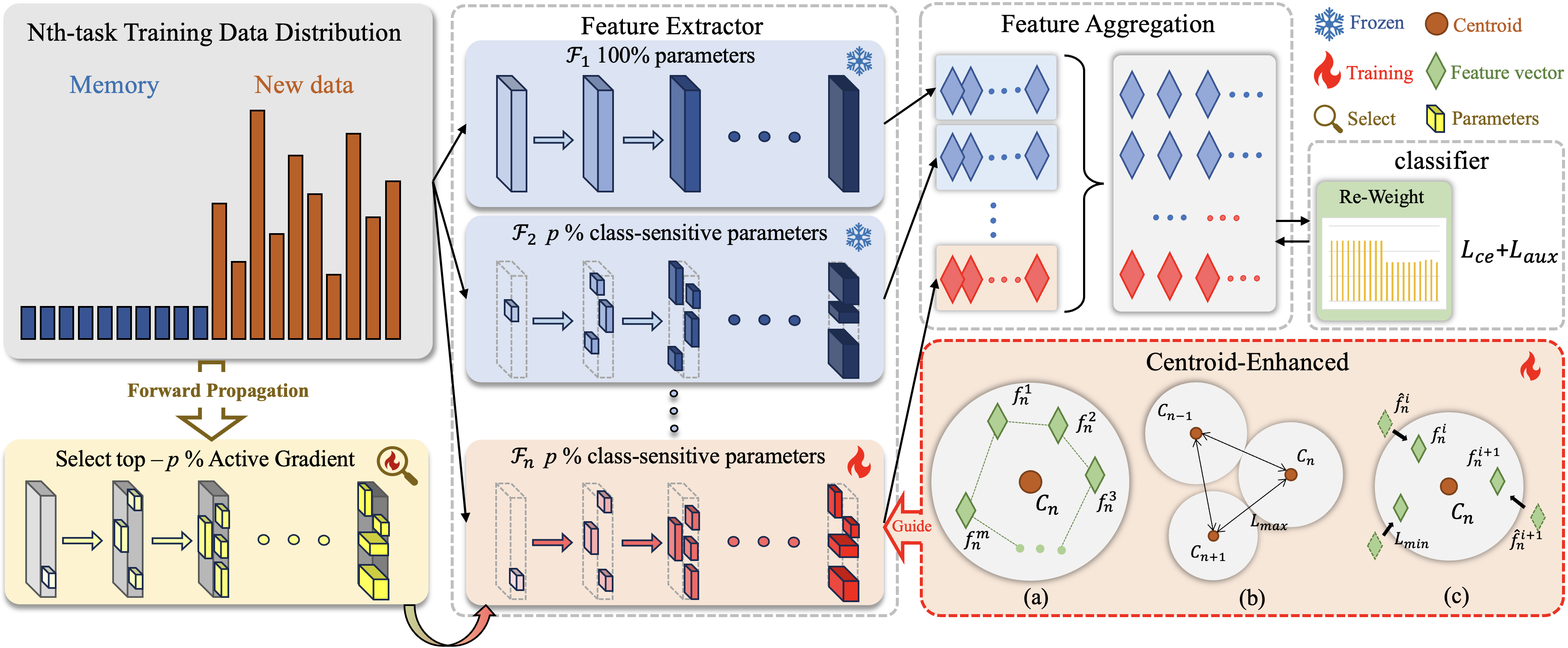
Figure 3: The overview of TaE. Note that the input for the current task comprises samples from the memory set and new data following a long-tailed distribution. During training for the $n$-th task, the training set undergoes multiple forward passes on the model from the previous round. It selects the most active p$\%$ of gradients (e.g., 5$\%$, 10$\%$, 20$\%$, 30$\%$) associated with these parameters, expands these selected parameters, and freezes the others. The learning process is guided by the Centroid-Enhanced (CEd) method: (a) each class learns a centroid updated throughout training; (b) centroids between different classes remain distant; (c) features within the same class converge towards the centroid. This process is governed by the $\mathcal{L}_{max-min}$ loss. Classifier learning is trained by the Re-weight strategy.

3.2 Extraction and Expansion of a Task-Aware Parameters

Recent research has observed that the pre-trained backbone exhibits distinct feature patterns at different locations [19, 15]. When confronted with downstream tasks, it is unnecessary to completely retrain all parameters. Instead, adjusting the domain-specific parameters based on the features of different task data proves more effective than a full retraining approach [5]. Inspired by this, the domains between new and old tasks are closely related (e.g., both involving image classification tasks) in CIL, and leveraging the characteristics of dynamic network methods, we treat the model learned in the $t$-1-th task as the ”pre-trained network” for the $t$ task. Consequently, we propose a novel Task-aware Expandable framework, which selects task-aware parameters for expansion and freezes the majority of parameters to mitigate forgetting.

Formally, given the training dataset $D^{t}$ for the $t$-th task, and the $t-1$ task model $\mathcal{F}_{t-1}$. We initially pass $D^{t}$ through the $\mathcal{F}_{0\cup t-1}$. Through multiple iterations involving forward propagation, we compute the gradient of each parameter and accumulate the changes in gradients over several loops, and the parameters are sorted based on their magnitudes. Finally, the top $p$$\%$ (e.g., 5$\%$, 10$\%$, 20$\%$, 30$\%$) of the most sensitive parameters are selected. The algorithmic process is illustrated in Algorithm 1.

Algorithm 1 Select Top-p$\%$ Most Sensitive Parameters

1:Input: $t$-th task data $\mathcal{D}^{t}$, Top percentage $p$, Iteration $Z$

2:Require: $\theta$ // parameter of $\mathcal{F}_{0\cup t-1}$

3:Output: Top $p\%$ sensitive parameters

4:for $i=1$ to $n$ do

5:     for $(\mathbf{x}_{i}^{t},y_{i}^{t})\in\mathcal{D}^{t}$ do

6:         Perform forward pass: $\mathcal{F}_{0\cup t-1}(\mathbf{x}_{i}^{t})\rightarrow\hat{y}_{i}$

7:         Compute $\mathcal{L}_{ce}$ by Eq 1

8:         Compute gradients: $\nabla\theta_{i}=\frac{\partial\mathcal{L}_{ce}}{\partial\theta}$

9:         Accumulate gradients: $\text{G}_{\theta}=\text{G}_{\theta}+\nabla\theta_{i}$

10:     end for

11:end for

12:Average accumulated gradients: $\bar{\text{G}_{\theta}}=\frac{\text{G}_{\theta}}{Z}$

13:Sort parameters based on gradient magnitude

14:$\text{$\theta_{select}$}=\text{Top}(\text{G}_{\theta},p)$

15:return $\theta_{select}$

3.3 Centroid-Enhanced Method

Due to the issue of long-tailed distribution, the model often exhibits a bias towards the head classes, leading to a lack of learning from tail class samples. This results in the features of the tail class being less discriminative. This problem with tail classes becomes more pronounced in CIL. To tackle this issue, we introduce a Centroid-Enhanced (CEd) method designed to steer the model towards learning class-specific features. For each observed class, we establish a centroid by training and maintaining a set of centroids. We parameterize these centroids to make them adaptable, updating them concurrently with the model training process to address the challenge of the feature space evolving with the introduction of new data. Specifically, during the model training phase, we first calculate the center point of features for each class as its centroid. We defined two loss functions, the max loss, and min loss, to guide the updating of centroids and features. The min loss ensures that features within the same category are closer, while the max loss ensures different category centroids are distinct from each other [14, 23, 18].

For computing the similarity between feature vectors, we opt to use cosine similarity to measure distance [29], which is thus: $\cos(u,v)=\frac{u\cdot v}{\left\|u\right\|\left\|v\right\|}$ where $u$ and $v$ are two vectors, $\cdot$ represents the dot product, and $\left\|\cdot\right\|$ is the $L_{2}$ norm.

The min loss ensures that features from samples within the same class gravitate towards their corresponding class centroid. It can be mathematically represented as:

$$\mathcal{L}_{min,t}=-\frac{1}{\mathcal{D}^{t}}\sum_{i=1}^{\mathcal{D}^{t}}\cos(f(\mathbf{x}_{i}^{t}),c_{y_{i}^{t}})$$ (2)

where $f(\mathbf{x}_{i}^{t})$ is the features of sample $\mathbf{x}_{i}^{t}$ fitted by the model, $c_{y_{i}^{t}}$ is the centroid of label $y_{i}^{t}$.

The max loss ensures that centroids of different classes are distinct and separated in the feature space. The loss is defined as:

$$\mathcal{L}_{max,t}=\frac{1}{\mathcal{K}_{t}(\mathcal{K}_{t}-1)}\sum_{j=1}^{\mathcal{K}_{t}}\sum_{k\neq j}^{\mathcal{K}_{t}}\cos(c_{j}^{t},c_{k}^{t})$$ (3)

where $\mathcal{K}_{t}$ is the number of classes in task $t$.

The overall loss function at task $t$ is defined as:

$$\mathcal{L}_{all,t}=\gamma_{1}\mathcal{L}_{ce,t}+\gamma_{2}\mathcal{L}_{min,t}+\gamma_{3}\mathcal{L}_{max,t}$$ (4)

where $\gamma_{1}$, $\gamma_{2}$, and $\gamma_{3}$ are the hyper-parameter to control the effort of these losses.

3.4 Classifier Learning

Existing CIL research has observed the issue of data imbalance between the exemplars and new data. However, there is also a data imbalance among the new task data in LT-CIL. Therefore, we further refined the Re-weight strategy.

Specifically, for the training set of the current task, $\mathcal{E}\cup\mathcal{D}^{t}$, with a total of $\mathcal{K}_{t}$ classes and $i$-th class having a quantity of $k^{t}_{i}$ samples. The effective weight for each class is defined as:

$$w_{i}=\frac{1-\beta}{1-\beta^{k^{t}_{i}}}$$ (5)

where $\beta$ is a hyper-parameter that controls the weights of different classes, and $w_{i}$ represents the weight for the $i$-th class.

To focus the model more on the tail classes in the new task, we calculate an equally sized weight matrix $W^{t}$ using the same formula for the new task distribution. The weights for the old classes in $W^{t}$ are set to 1. Therefore, the normalized weight formula is:

$$\bar{w_{i}}=\frac{w_{i}}{\sum_{i=1}^{\mathcal{K}^{t}}w_{i}}\times W^{t}\times\mathcal{K}^{t}$$ (6)

4 EXPERIMENT

In this section, we conducted extensive experiments to validate the effectiveness of our approach. We tested our method on CIFAR100 [9] and Imagenet100 [22] datasets, incorporating commonly used data protocols and imbalanced ratio protocols. A series of ablation experiments were also performed to verify the effectiveness of each component. Additionally, we conducted experiments and discussions on extending the method to different data proportions. Furthermore, we integrated the CEd method with typical CIL algorithms to demonstrate the applicability of CEd to CIL algorithms. Due to page constraints, additional quantitative and qualitative analyses are available in Appendices A and B, respectively.

4.1 Experiment Setup and Implementation Details

Dataset	$\rho=0.1$	$\rho=0.05$	$\rho=0.01$
	H-T-M	H-T-M	H-T-M
CIFAR100	500-50-20	500-25-20	500-5-5
Imagenet100	1k-100-20	1k-50-20	1k-10-10

Table 1: Imbalanced Ratio Protocol, H-T-M means the number of head, tail, and memory, k means 1000.

Datasets. CIFAR-100 [9] is composed of 32x32 pixel color images classified into 100 classes. The dataset comprises 50,000 training images, with 500 images per class, and 10,000 evaluation images, featuring 100 images per class. ImageNet-100 [22] is curated by selecting 100 classes from the ImageNet-1000 dataset, which includes 100,000 training images, with 1,000 images per class, and 5,000 evaluation images, with 50 images per class.
Datasets Protocol: We follow the protocol introduced in [20], which involves training all 100 classes through multiple splits, encompassing 5, 10, and 20 incremental steps, while maintaining a fixed memory size of 2,000 exemplars across batches.
Imbalanced Ratio Protocol: We adopt three protocols for the head-to-tail sample count ratio in the long-tailed distribution: $\rho$ = 0.1, $\rho$ = 0.05, and $\rho$ = 0.01. In Table 5, the details of three protocols combined with two datasets are presented, including the sample counts for head and tail classes, as well as the sample quantities for each category stored in the memory.
Implementation Details: We implemented our method using PyTorch [16]. We applied a long-tailed transformation to both CIFAR-100 and ImageNet100. The experiments leveraged the public implementations of existing CIL methods within the PyCIL framework [37]. For CIFAR-100, we employed ResNet-32 [6], with an initial learning rate set at 0.1, which was reduced by a factor of 10 at epochs 80, 120, and 150 (out of a total of 170 epochs). For ImageNet100, we utilized ResNet-18 with the same learning rate adjustments. In these experiments, we choose exemplars for memory based on the herding selection strategy [28], in line with previous studies [20].

4.2 Evaluation on CIFAR100

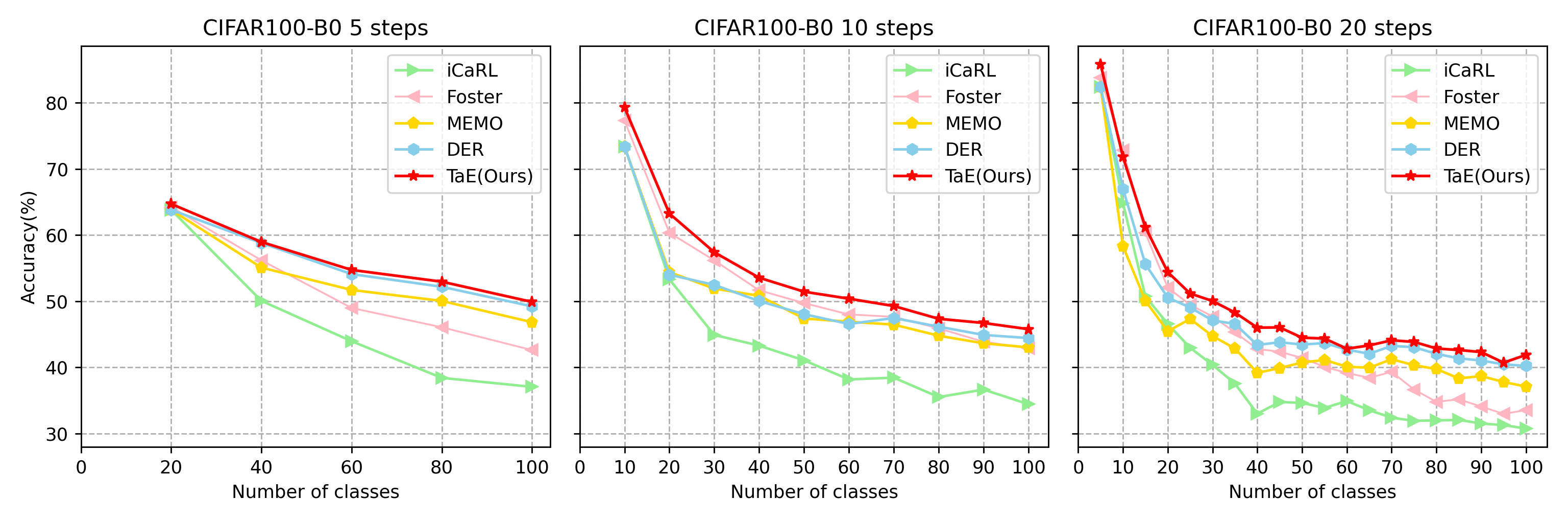
Figure 4: The performance for each step. The model is trained on CIFAR100 $\rho$ = 0.1 with three Datasets Protocols.

Method	$\rho=0.1$		$\rho=0.05$		$\rho=0.01$
	Last	Avg	Last	Avg	Last	Avg
Finetune	7.8	22.42	7.57	20.98	5.83	15.36
EWC	8.88	22.37	8.45	20.98	5.63	14.92
LwF	16.82	33.51	16.94	28.45	11.56	20.39
iCaRL	34.43	44.82	33.63	41.64	14.32	22.68
Foster	42.89	53.82	39.86	47.28	15.17	21.72
MEMO	43.02	50.94	40.08	46.31	21.0	26.39
DER	44.43	50.74	39.24	44.37	22.89	28.44
TaE($p$=30$\%$)	46.84	54.43	40.87	48.29	23.54	29.69

Table 2: Performance comparison of typical CIL algorithms on CIFAR100 B0-10steps benchmarks, evaluated across three Imbalanced Ratio Protocols.

Quantitative Results Table 2 and Figure 4 summarize the results of the CIFAR-100 benchmark tests. We utilized typical CIL algorithms such as iCaRL [20], DER [31], Foster [25], and MEMO [36] as baseline methods. The experimental results reveal that DER, MEMO, and Foster, as state-of-the-art algorithms, fail to consistently exhibit robust performance across different experimental setups. This observation supports Liu et al.’s proposition that LT-CIL may compromise the robustness of traditional CIL methods [13]. For instance, under the same setting with $p\rho=0.1$ and varying data protocols, Foster performs less effectively than DER and MEMO, particularly showing a significant decline in the B0-20 steps scenario. Conversely, under the same B0-10 steps setting but with different imbalanced ratio protocols, Foster achieves a higher average accuracy compared to DER and MEMO. We attribute this to Foster’s inherent Re-weight strategy, intended to balance the exemplar set and new data. MEMO’s strategy of expanding only task-specific blocks approximates a $30\%$ backbone expansion. The experimental results demonstrate that, under similar parameter expansion, TaE’s task-aware parameter expansion is more suitable for LT-CIL scenarios. The experimental results indicate that our approach outperforms other methods across all six settings in the CIFAR-100 dataset, which substantiates the strong robustness of our method.

4.3 Evaluation in Imagenet100

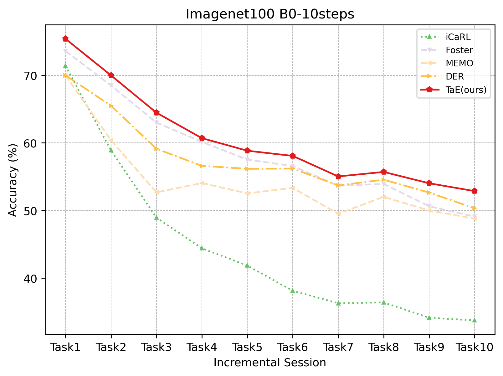
Figure 5: The performance for each step. The model is trained on Imagenet100 B0-10steps $\rho$ = 0.1

Quantitative Results In the Imagenet100 experiments, we observe experimental phenomena similar to those in CIFAR100. Figure 10 illustrates the accuracy of different methods at each incremental stage, revealing our approach consistently outperforms others. Specifically, our method achieves a 2.54$\%$ higher accuracy in the final stage compared to the second-best method. Concerning average accuracy, the closest competitor is the Foster method; however, the TaE method surpasses Foster’s average accuracy by 0.97$\%$ and exceeds other methods by at least 3$\%$. Additional experimental results can be found in Appendix B.

4.4 Ablation Study

RW	$\mathcal{L}_{max-min}$	Last	Avg
✗	✗	45.03	51.92
✓	✗	45.79	53.08
✓	✓	46.84	54.43

Table 3: Ablations of key components in TaE($30\%$). We report the average and last accuracy on CIFAR100 B0-10 steps. RW means Re-Weight strategy.

To validate the effectiveness of each component in TaE, we conducted an ablation study on CIFAR100 B10-10steps with $\rho$ = 0.1. As shown in Tab.3, both the average and final accuracy progressively improved as we added more components. We observe that, building upon TaE($30\%$), the inclusion of Re-weight results in an average accuracy improvement of $1.16\%$, and further incorporating $\mathcal{L}_{max-min}$ leads to an additional average accuracy enhancement of $1.35\%$.

4.5 Discussion on the Selection of Parameter Ratios

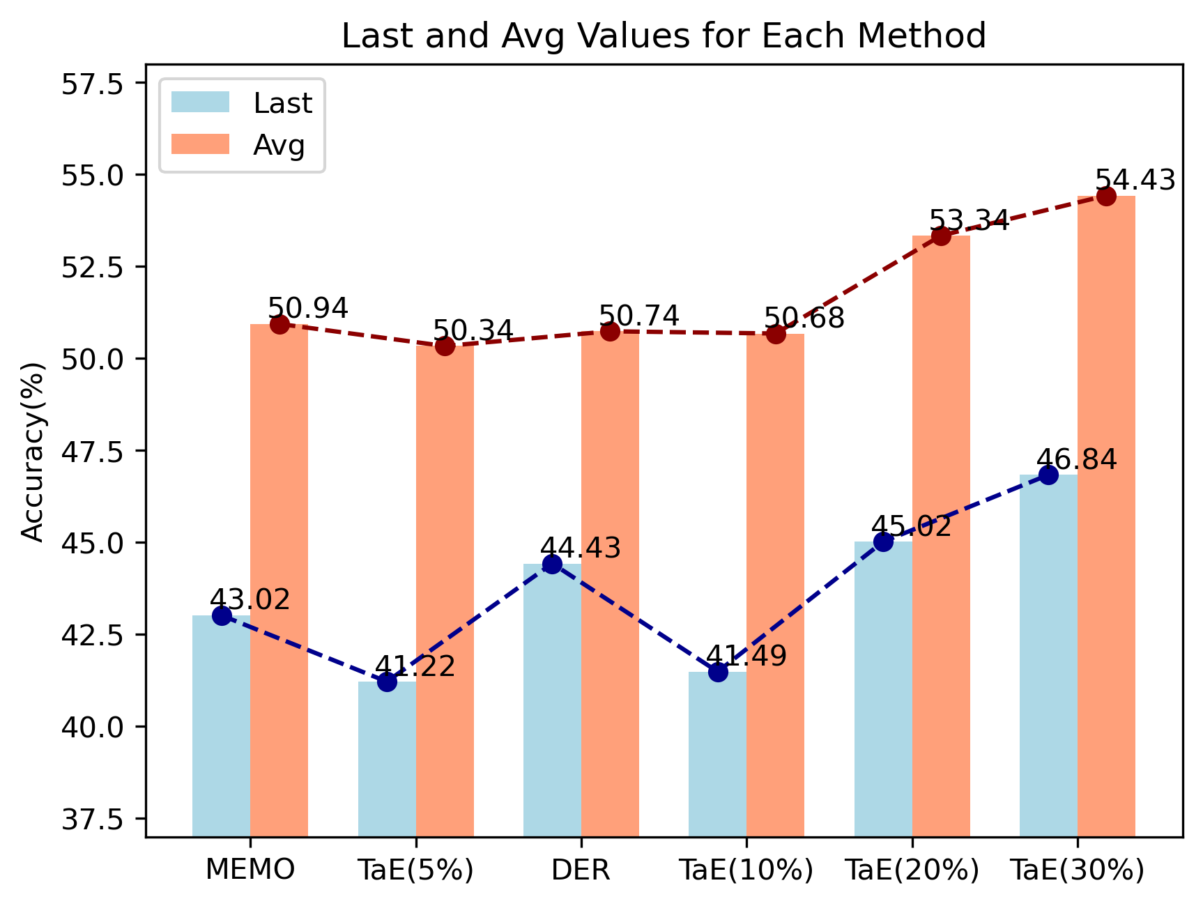
Figure 6: The Last and Average Accuracy. We compare our model($p$ = 5$\%$, 10$\%$, 20$\%$, 30$\%$) with SOTA CIL methods (DER and MEMO), and the model trained on the experiment CIFAR100 B0-10 steps with $\rho=0.1$

.

In this section, we conducted experiments on the Imagenet100 and CIFAR100 datasets using the B0-10steps benchmark with $p=0.1$, comparing the performance of TaE ($p=5\%,10\%,20\%,30\%$) with MEMO and DER. As shown in Figure 1, when training the model on Imagenet100, the performance of TaE increases with higher values of $p$. TaE surpasses MEMO at $p=5\%$ and exceeds DER at $p=10\%$. TaE($30\%$) outperforms MEMO in terms of both final accuracy and average accuracy, achieving a superiority of $4.08\%$ and $5.00\%$, respectively. Moreover, compared to DER, TaE($30\%$) exhibits a superiority of $2.54\%$ in final accuracy and $2.25\%$ in average accuracy.

However, as illustrated in Figure 6, when training the model on CIFAR100, TaE only surpasses DER and MEMO at $p=20\%$. TaE($30\%$) surpasses MEMO in both final accuracy and average accuracy, demonstrating advantages of $3.82\%$ and $3.39\%$, respectively. Additionally, in comparison to DER, TaE($30\%$) demonstrates a superiority of $2.41\%$ in final accuracy and $3.71\%$ in average accuracy.

The experimental results suggest that treating the model from the previous stage as the ”pre-trained” model for the current stage and performing task-aware fine-tuning on it is reasonable. Moreover, as the expansion ratio increases, the performance of TaE also shows a corresponding improvement. However, in the experimental setup using CIFAR100, the enhancement of TaE from 5$\%$ to 10$\%$ is not pronounced, whereas the improvement becomes more evident from 10$\%$ to 20$\%$, and further from 20$\%$ to 30$\%$. In the experimental configuration with Imagenet100, the accuracy improvement is consistently steady, indicating that incremental models trained on CIFAR100 require a more extensive parameter expansion for new tasks. We attribute this experimental phenomenon to the fact that Imagenet100 exhibits more pixel information and a greater number of category samples compared to CIFAR100, thereby endowing the model with stronger representational capabilities. Additionally, beyond a certain $p\%$, the model’s performance experiences a decline. More detailed experiments can be found in Appendix A.

4.6 Effectiveness of Centroid-Enhanced Method

Method	B0-5 steps		B0-10 steps		B0-20 steps
	Last	Avg	Last	Avg	Last	Avg
LwF	8.15	23.12	17.56	32.87	27.02	40.09
w CEd	8.86	24.23	17.84	33.79	30.99	41.22
iCarL	37.05	46.51	34.13	43.47	30.74	39.59
w CEd	43.76	52.35	41.24	51.95	33.35	43.51
DER	46.26	52.91	44.43	50.74	39.70	46.31
w CEd	48.51	56.50	45.07	53.23	40.05	47.52
Foster	41.82	51.46	40.44	51.23	35.03	45.51
w CEd	42.08	51.73	40.98	52.67	36.97	48.12

Table 4: Performance comparison of four CIL algorithms combined with CEd on the CIFAR100 $\rho$ = 0.1 benchmarks, evaluated across three Datasets Protocols.

Method	$\rho=0.1$		$\rho=0.05$		$\rho=0.01$
	Last	Avg	Last	Avg	Last	Avg
LwF	17.84	38.02	17.84	34.53	12.72	24.90
w CEd	19.60	39.45	18.04	36.04	14.18	25.96
iCarL	33.72	44.40	32.98	42.51	15.78	23.49
w CEd	43.26	53.96	40.84	49.41	23.62	27.02
DER	50.32	57.48	50.32	56.04	29.86	32.68
w CEd	54.82	60.90	51.14	57.26	31.16	36.50
Foster	49.08	59.14	44.70	53.35	17.28	22.72
w CEd	51.34	60.44	45.26	54.89	18.10	23.64

Table 5: Performance comparison of four CIL algorithms combined with CEd on the Imagenet100 B10-10 steps, evaluated across three Imbalanced Ratio Protocols.

The centroid-enhanced(CEd) method can be applied to most ”training from sketch” CIL methods. In this section, we will validate the effectiveness of the centroid set in various experimental settings. In Table 4, we present the experimental results on the CIFAR100 with $\rho$ = 0.1. We applied CEd to four representative CIL methods. Our experiments were conducted under three different protocols: B0-5steps, B0-10steps, and B0-20steps. In Table 5, we display the experimental results on the Imagenet100 dataset. Three different long-tail ratios were set with the same B0-10 steps. Similar to Table 4, we compared the accuracy of the last task and the average accuracy.

The experimental results reveal that the inclusion of the centroid set enhances the performance of four representative CIL methods. We can observe improvements across various benchmarks for all four CIL methods after the incorporation of the CEd approach. Particularly, in the experimental setup of iCaRL with B0-10 steps, the final accuracy and average accuracy in the last stage increased by $7.11\%$ and $8.48\%$, respectively. The average accuracy even surpasses that of DER and Foster under the same experimental conditions. In other benchmarks, the improvement of iCaRL is notably pronounced. Additionally, the observed improvement upon combining CEd with Foster, given Foster’s inherent Re-weight strategy, serves as a supportive ablation study validating the effectiveness of CEd. The above experiments demonstrate that our proposed centroid method effectively strengthens the ability of CIL to handle LT-CIL.

5 Conclusions

In this study, we introduce a task-aware expandable framework to address the challenges in long-tail class incremental learning. We select the most gradient-sensitive parameters within the last-step model through forward propagation before each training task. By selectively expanding and training selected parameters, we effectively enhance the model’s representational capabilities without memory explosion. Additionally, we propose a centroid-enhanced method to guide the training of task-aware parameters, which is adaptable to most class-incremental learning methods, encouraging the model to acquire more class-specific feature representation. The efficacy of our approach was rigorously evaluated through exhaustive experimentation conducted across two datasets, utilizing three data protocols and three imbalance ratio protocols. The experimental results highlight the superiority of our method in the long-tailed class incremental learning and our method achieves remarkable outcomes with the expansion of only a light subset of task-aware parameters. We believe that our work will pave the way for future research in long-tailed class-incremental learning.

Supplementary Material

Appendix A Hyperparameters

We conducted experiments on CIFAR100 and Imagenet B0-10 steps with $\rho=0.1$ as illustrated in Figure 7 and Figure 8, providing a detailed comparison of the accuracy of task-aware parameters at different expansion ratios. Experimental results reveal that, under the CIFAR100 settings, the algorithm’s performance steadily improves from 5$\%$ to 30$\%$, beyond which the accuracy remains stable. In the Imagenet100 settings, the algorithm’s performance progressively increases from 5$\%$ to 40$\%$, reaching its peak after 40$\%$. This demonstrates that the models require only a small number of task-aware parameters to achieve State-of-the-Art performance, while further expansion of parameters results in redundancy.

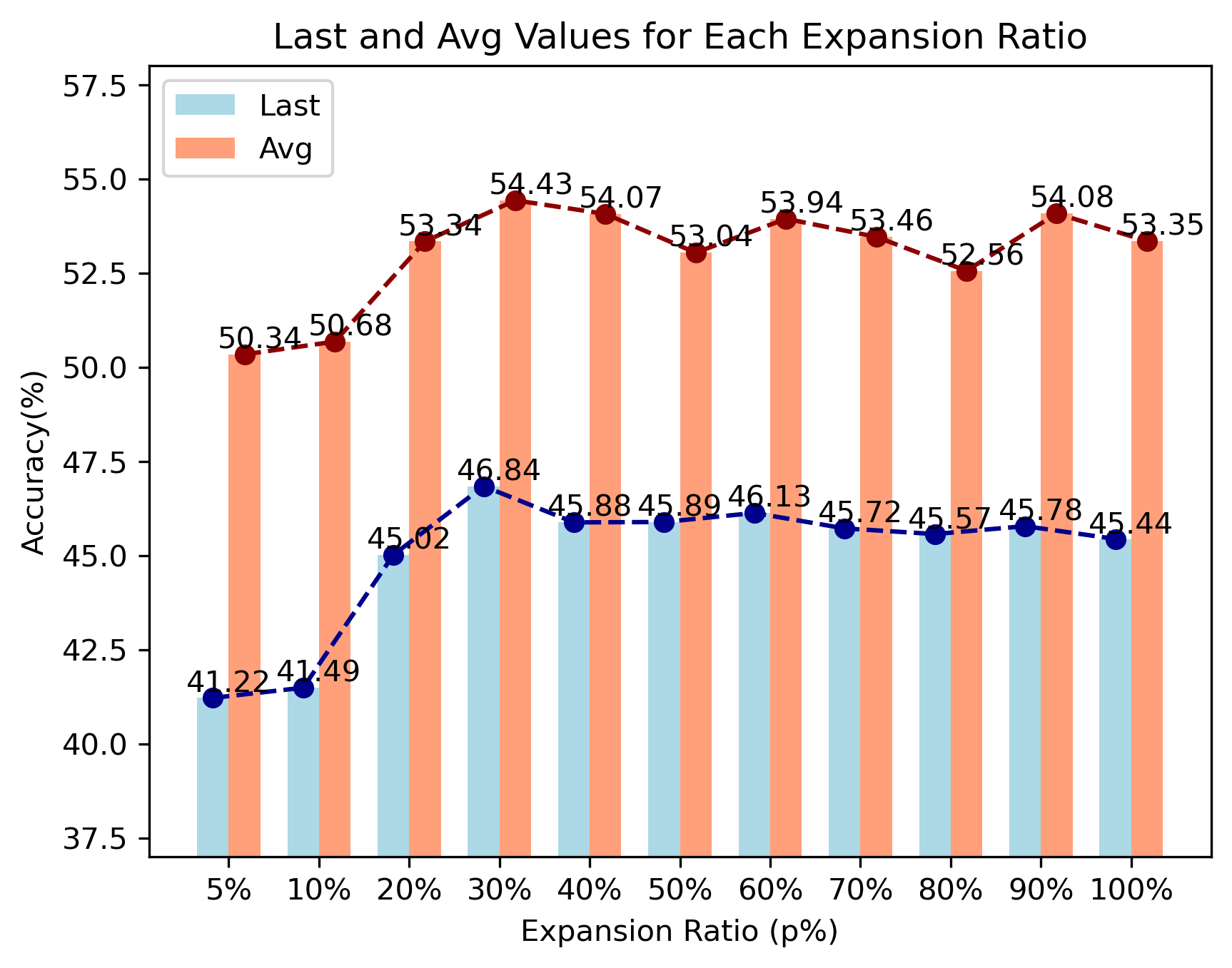
Figure 7: The Last and Average Accuracy. We compare our model($p$ = 5$\%$, 10$\%$, 20$\%$, 30$\%$, 40$\%$, 50$\%$, 60$\%$, 70$\%$, 80$\%$, 90$\%$, 100$\%$) and the model trained on the experiment CIFAR100 B0-10steps with $\rho=0.1$.

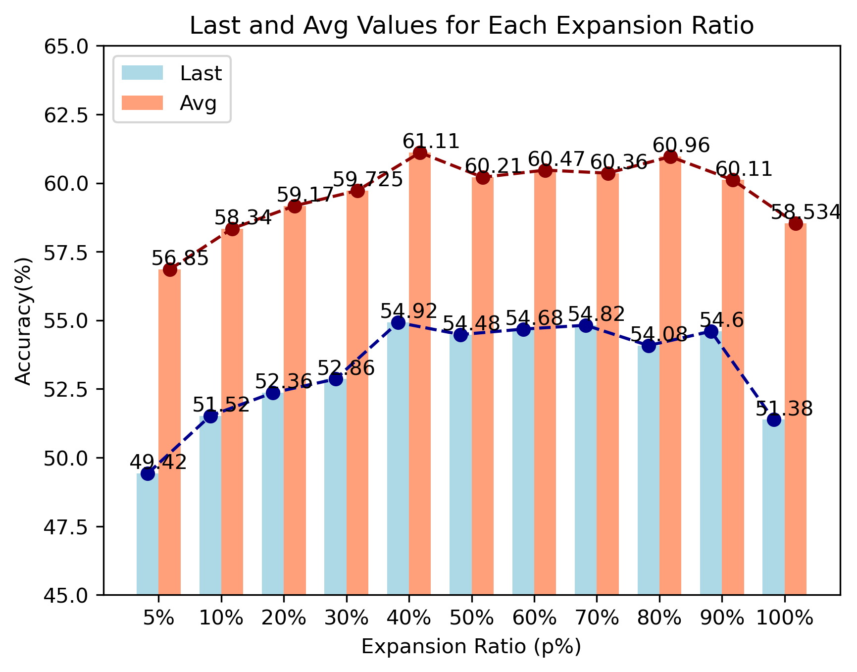
Figure 8: The Last and Average Accuracy. We compare our model($p$ = 5$\%$, 10$\%$, 20$\%$, 30$\%$, 40$\%$, 50$\%$, 60$\%$, 70$\%$, 80$\%$, 90$\%$, 100$\%$) and the model trained on the experiment Imagenet100 B0-10steps with $\rho=0.1$.

We conducted a sensitivity analysis on the hyperparameters in the Eq 4. For simplicity, we set $\gamma_{1}$ to 1 and explored various combinations of $\gamma_{2}$ and $\gamma_{2}$ to assess the importance of $\mathcal{L}_{min}$ and $\mathcal{L}_{max}$. From the experimental results, it is evident that the performance of all hyperparameter combinations surpasses that of the State-of-the-Art method, confirming the robustness of TaE. When the value of $\gamma_{2}$ and $\gamma_{2}$ are close, and the model slightly leans towards emphasizing inter-class distances, the best performance is achieved. The results show a final accuracy of 47.19$\%$ and an average accuracy of 54.72$\%$, surpassing the SOTA by 2.76$\%$ and 3.98$\%$, respectively.

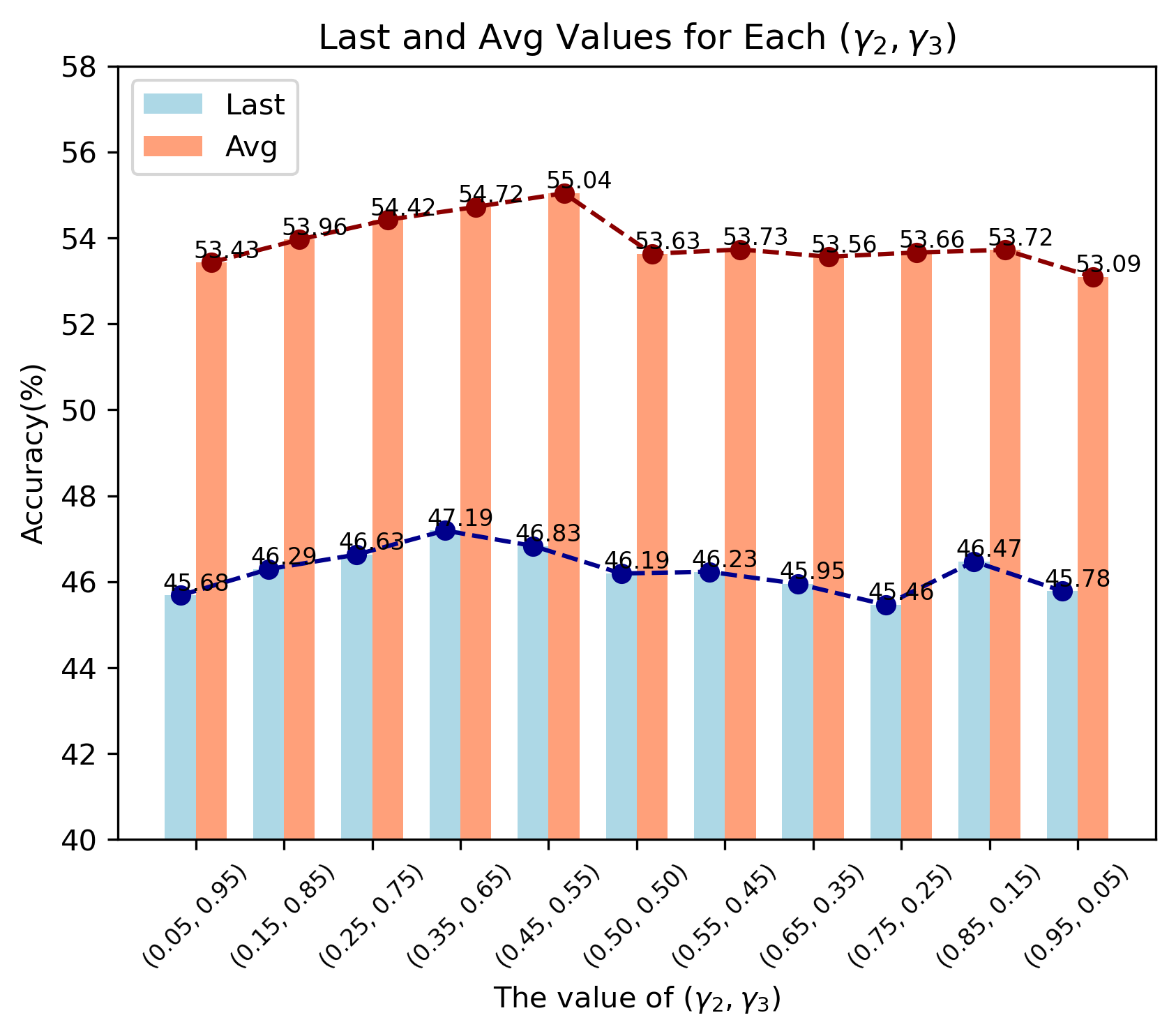
Figure 9: The Last and Average Accuracy. We compare our model($p$ = 30$\%$) across various combinations of $\mathcal{L}_{max}$ and $\mathcal{L}_{min}$. and the model trained on the experiment CIFAR100 B0-10steps with $\rho=0.1$.

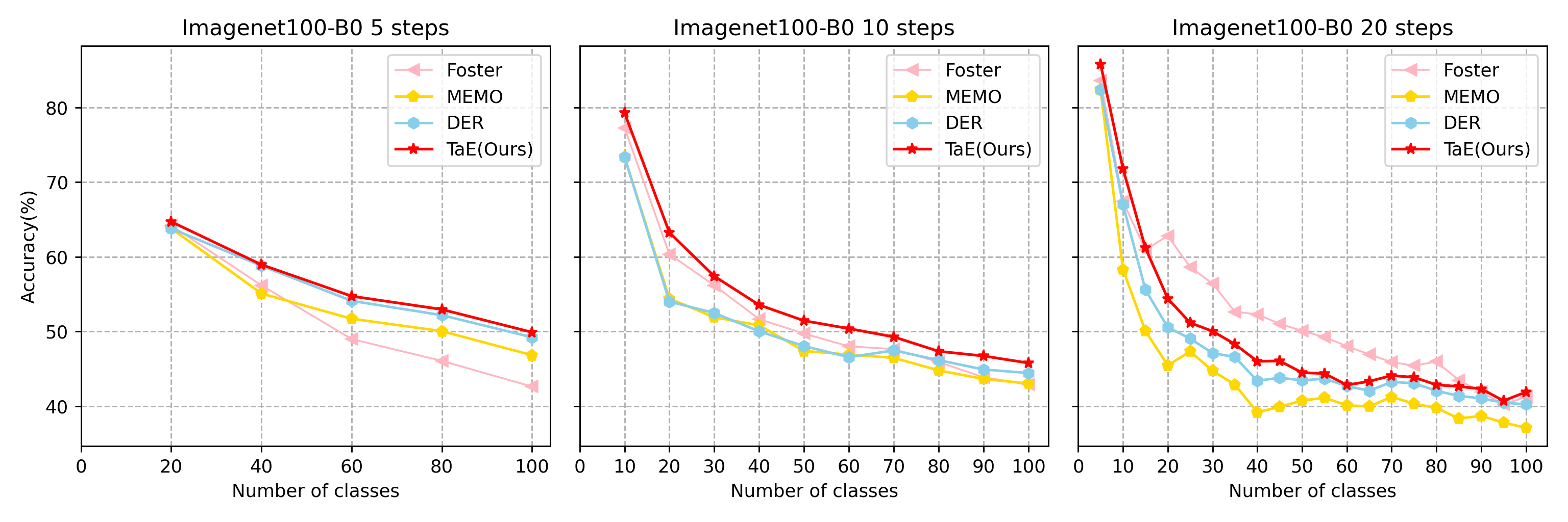
Figure 10: The performance for each step. The model is trained on Imagenet100 $\rho$ = 0.1 with three Datasets Protocols.

Method	$\rho=0.1$		$\rho=0.05$		$\rho=0.01$
	Last	Avg	Last	Avg	Last	Avg
LwF	19.60	38.76	18.04	34.67	14.18	20.39
iCaRL	33.72	44.40	32.98	42.51	15.78	23.49
Foster	49.08	59.15	44.07	50.40	18.10	23.12
MEMO	48.78	54.73	44.10	50.395	25.72	30.47
DER	50.32	57.48	41.22	50.69	26.82	31.22
TaE($p$=30$\%$)	52.86	59.73	44.69	55.28	29.98	33.75

Table 6: Performance comparison of typical CIL algorithms on Imagenet100 B0-10steps benchmarks, evaluated across three Imbalanced Ratio Protocols.

Appendix B More detailed results on Imagenet100

This section provides a more detailed experiment conducted on Imagenet100. Figure 10 illustrates the performance of various methods under three different dataset protocols. It is evident that, except for Foster’s performance in the middle steps of the B0-20 steps, the remaining TaE methods consistently achieve optimal performance. Table 6 presents the performance of different methods under three distinct long-tail ratio settings, with TaE consistently demonstrating the best performance across all scenarios.

References

- Cao et al. [2019] Kaidi Cao, Colin Wei, Adrien Gaidon, Nikos Arechiga, and Tengyu Ma. Learning imbalanced datasets with label-distribution-aware margin loss. Advances in neural information processing systems, 32, 2019.
- Chu et al. [2020] Peng Chu, Xiao Bian, Shaopeng Liu, and Haibin Ling. Feature space augmentation for long-tailed data. In Computer Vision–ECCV 2020: 16th European Conference, Glasgow, UK, August 23–28, 2020, Proceedings, Part XXIX 16, pages 694–710. Springer, 2020.
- Douillard et al. [2020] Arthur Douillard, Matthieu Cord, Charles Ollion, Thomas Robert, and Eduardo Valle. Podnet: Pooled outputs distillation for small-tasks incremental learning. In Computer Vision–ECCV 2020: 16th European Conference, Glasgow, UK, August 23–28, 2020, Proceedings, Part XX 16, pages 86–102. Springer, 2020.
- French [1999] Robert M French. Catastrophic forgetting in connectionist networks. Trends in cognitive sciences, 3(4):128–135, 1999.
- He et al. [2023] Haoyu He, Jianfei Cai, Jing Zhang, Dacheng Tao, and Bohan Zhuang. Sensitivity-aware visual parameter-efficient tuning. arXiv preprint arXiv:2303.08566, 2023.
- He et al. [2016] Kaiming He, Xiangyu Zhang, Shaoqing Ren, and Jian Sun. Identity mappings in deep residual networks. In Computer Vision–ECCV 2016: 14th European Conference, Amsterdam, The Netherlands, October 11–14, 2016, Proceedings, Part IV 14, pages 630–645. Springer, 2016.
- Kang et al. [2019] Bingyi Kang, Saining Xie, Marcus Rohrbach, Zhicheng Yan, Albert Gordo, Jiashi Feng, and Yannis Kalantidis. Decoupling representation and classifier for long-tailed recognition. arXiv preprint arXiv:1910.09217, 2019.
- Kirkpatrick et al. [2017] James Kirkpatrick, Razvan Pascanu, Neil Rabinowitz, Joel Veness, Guillaume Desjardins, Andrei A Rusu, Kieran Milan, John Quan, Tiago Ramalho, Agnieszka Grabska-Barwinska, et al. Overcoming catastrophic forgetting in neural networks. Proceedings of the national academy of sciences, 114(13):3521–3526, 2017.
- Krizhevsky et al. [2009] Alex Krizhevsky, Geoffrey Hinton, et al. Learning multiple layers of features from tiny images. 2009.
- Li and Hoiem [2017] Zhizhong Li and Derek Hoiem. Learning without forgetting. IEEE transactions on pattern analysis and machine intelligence, 40(12):2935–2947, 2017.
- Lin et al. [2017] Tsung-Yi Lin, Priya Goyal, Ross Girshick, Kaiming He, and Piotr Dollár. Focal loss for dense object detection. In Proceedings of the IEEE international conference on computer vision, pages 2980–2988, 2017.
- Liu et al. [2021] Bo Liu, Haoxiang Li, Hao Kang, Gang Hua, and Nuno Vasconcelos. Gistnet: a geometric structure transfer network for long-tailed recognition. In Proceedings of the IEEE/CVF International Conference on Computer Vision, pages 8209–8218, 2021.
- Liu et al. [2022] Xialei Liu, Yu-Song Hu, Xu-Sheng Cao, Andrew D Bagdanov, Ke Li, and Ming-Ming Cheng. Long-tailed class incremental learning. In European Conference on Computer Vision, pages 495–512. Springer, 2022.
- Martinetz et al. [1991] Thomas Martinetz, Klaus Schulten, et al. A” neural-gas” network learns topologies. 1991.
- Muzammal et al. [2021] Naseer Muzammal, Ranasinghe Kanchana, H Khan Salman, Hayat Munawar, Shahbaz Khan Fahad, and Yang Ming-Hsuan. Intriguing properties of vision transformers. arXiv preprint arXiv:2105.10497, 3, 2021.
- Paszke et al. [2017] Adam Paszke, Sam Gross, Soumith Chintala, Gregory Chanan, Edward Yang, Zachary DeVito, Zeming Lin, Alban Desmaison, Luca Antiga, and Adam Lerer. Automatic differentiation in pytorch. 2017.
- Perez and Wang [2017] Luis Perez and Jason Wang. The effectiveness of data augmentation in image classification using deep learning. arXiv preprint arXiv:1712.04621, 2017.
- Prudent and Ennaji [2005] Yann Prudent and Abdellatif Ennaji. An incremental growing neural gas learns topologies. In Proceedings. 2005 IEEE International Joint Conference on Neural Networks, 2005., pages 1211–1216. IEEE, 2005.
- Raghu et al. [2021] Maithra Raghu, Thomas Unterthiner, Simon Kornblith, Chiyuan Zhang, and Alexey Dosovitskiy. Do vision transformers see like convolutional neural networks? Advances in Neural Information Processing Systems, 34:12116–12128, 2021.
- Rebuffi et al. [2017] Sylvestre-Alvise Rebuffi, Alexander Kolesnikov, Georg Sperl, and Christoph H Lampert. icarl: Incremental classifier and representation learning. In Proceedings of the IEEE conference on Computer Vision and Pattern Recognition, pages 2001–2010, 2017.
- Rousseeuw [1987] Peter J Rousseeuw. Silhouettes: a graphical aid to the interpretation and validation of cluster analysis. Journal of computational and applied mathematics, 20:53–65, 1987.
- Russakovsky et al. [2015] Olga Russakovsky, Jia Deng, Hao Su, Jonathan Krause, Sanjeev Satheesh, Sean Ma, Zhiheng Huang, Andrej Karpathy, Aditya Khosla, Michael Bernstein, et al. Imagenet large scale visual recognition challenge. International journal of computer vision, 115:211–252, 2015.
- Tao et al. [2020] Xiaoyu Tao, Xiaopeng Hong, Xinyuan Chang, Songlin Dong, Xing Wei, and Yihong Gong. Few-shot class-incremental learning. In Proceedings of the IEEE/CVF Conference on Computer Vision and Pattern Recognition, pages 12183–12192, 2020.
- Wang et al. [2022a] Fu-Yun Wang, Da-Wei Zhou, Liu Liu, Han-Jia Ye, Yatao Bian, De-Chuan Zhan, and Peilin Zhao. Beef: Bi-compatible class-incremental learning via energy-based expansion and fusion. In The Eleventh International Conference on Learning Representations, 2022a.
- Wang et al. [2022b] Fu-Yun Wang, Da-Wei Zhou, Han-Jia Ye, and De-Chuan Zhan. Foster: Feature boosting and compression for class-incremental learning. In European conference on computer vision, pages 398–414. Springer, 2022b.
- Wang et al. [2019] Yiru Wang, Weihao Gan, Jie Yang, Wei Wu, and Junjie Yan. Dynamic curriculum learning for imbalanced data classification. In Proceedings of the IEEE/CVF international conference on computer vision, pages 5017–5026, 2019.
- Wang et al. [2017] Yu-Xiong Wang, Deva Ramanan, and Martial Hebert. Learning to model the tail. Advances in neural information processing systems, 30, 2017.
- Welling [2009] Max Welling. Herding dynamical weights to learn. In Proceedings of the 26th Annual International Conference on Machine Learning, pages 1121–1128, 2009.
- Xia et al. [2015] Peipei Xia, Li Zhang, and Fanzhang Li. Learning similarity with cosine similarity ensemble. Information sciences, 307:39–52, 2015.
- Xiang et al. [2020] Liuyu Xiang, Guiguang Ding, and Jungong Han. Learning from multiple experts: Self-paced knowledge distillation for long-tailed classification. In Computer Vision–ECCV 2020: 16th European Conference, Glasgow, UK, August 23–28, 2020, Proceedings, Part V 16, pages 247–263. Springer, 2020.
- Yan et al. [2021] Shipeng Yan, Jiangwei Xie, and Xuming He. Der: Dynamically expandable representation for class incremental learning. In Proceedings of the IEEE/CVF Conference on Computer Vision and Pattern Recognition, pages 3014–3023, 2021.
- Yin et al. [2019] Xi Yin, Xiang Yu, Kihyuk Sohn, Xiaoming Liu, and Manmohan Chandraker. Feature transfer learning for face recognition with under-represented data. In Proceedings of the IEEE/CVF conference on computer vision and pattern recognition, pages 5704–5713, 2019.
- Zhang et al. [2021] Songyang Zhang, Zeming Li, Shipeng Yan, Xuming He, and Jian Sun. Distribution alignment: A unified framework for long-tail visual recognition. In Proceedings of the IEEE/CVF conference on computer vision and pattern recognition, pages 2361–2370, 2021.
- Zhang et al. [2023] Yifan Zhang, Bingyi Kang, Bryan Hooi, Shuicheng Yan, and Jiashi Feng. Deep long-tailed learning: A survey. IEEE Transactions on Pattern Analysis and Machine Intelligence, 2023.
- Zhou et al. [2020] Boyan Zhou, Quan Cui, Xiu-Shen Wei, and Zhao-Min Chen. Bbn: Bilateral-branch network with cumulative learning for long-tailed visual recognition. In Proceedings of the IEEE/CVF conference on computer vision and pattern recognition, pages 9719–9728, 2020.
- Zhou et al. [2022] Da-Wei Zhou, Qi-Wei Wang, Han-Jia Ye, and De-Chuan Zhan. A model or 603 exemplars: Towards memory-efficient class-incremental learning. arXiv preprint arXiv:2205.13218, 2022.
- Zhou et al. [2023a] Da-Wei Zhou, Fu-Yun Wang, Han-Jia Ye, and De-Chuan Zhan. Pycil: A python toolbox for class-incremental learning, 2023a.
- Zhou et al. [2023b] Da-Wei Zhou, Qi-Wei Wang, Zhi-Hong Qi, Han-Jia Ye, De-Chuan Zhan, and Ziwei Liu. Deep class-incremental learning: A survey. arXiv preprint arXiv:2302.03648, 2023b.