The $\phi^{n}$ trajectory bootstrap

Abstract

The Green’s functions $G_{n}=\left\langle\phi^{n}\right\rangle$ and their self-consistent equations admit analytic continuations to complex $n$. The indeterminacy of bootstrap problems can be resolved by the principle of minimal singularity. We use the harmonic oscillator to illustrate various aspects of the bootstrap analysis, such as the large $n$ expansion, matching conditions, exact quantization condition, and high energy asymptotic behavior. For the Hermitian quartic and non-Hermitian cubic oscillators, we revisit the $\phi^{n}$ trajectories at non-integer $n$ by the standard wave function formulation. The results are in agreement with the minimally singular solutions. Using the matching procedure, we obtain accurate solutions for anharmonic oscillators with higher powers. In particular, the existence of $G_{n}$ with non-integer $n$ allows us to bootstrap the $\mathcal{PT}$ invariant oscillators with non-integer powers.

1 Introduction

Self-consistent equations imply that physical observables are closely related to each other. It is natural to package the set of self-consistent observables as a mathematical function. What kind of properties should be expected for this function? Historically, the developments of the bootstrap approach to the strong interaction were deeply intertwined with analytic properties Regge:1959mz ; Chew:book ; Chew:1961ev . In complex analysis, analyticity also implies some self-consistent constraints for complex functions. From a local perspective, the Cauchy-Riemann equations ensure that the complex derivative is given by a path-independent limit. From a non-local perspective, the results of analytic continuations are path independent as long as there is no obstruction to path deformation. Analyticity is both elegant and powerful.

The bootstrap approach is not without blemish. Typically, the self-consistent constraints form an underdetermined system. In perturbation theory, it may appear that the self-consistent equations can be solved order by order. Unfortunately, it is usually not the case in nonperturbative studies. To make more definite predictions, one needs to introduce additional assumptions, such as basic principles and educated ansatz. Analogously, analyticity itself does not lead to unambiguous functions. In fact, a nontrivial function cannot be analytic everywhere. Analyticity should be supplemented with the properties of the singularity structure, which encode additional information and thus eliminate the ambiguities. In Li:2023ewe , we proposed that the indeterminacy of bootstrap problems can be resolved by the principle of minimal singularity, i.e. the complexity of the singularity structure should be minimized.

For illustration, let us consider the zero-dimensional scalar field theories. In $D=(0+0)$ dimensions, there is only one point in space and no time evolution. The basic observables are the Green’s functions $G_{n}=\left\langle\phi^{n}\right\rangle$ with positive integer $n$. We can package these observables by viewing $G_{n}$ as a function of $n$. On one hand, $G_{n}$ is not an arbitrary function due to the self-consistent constraints from the Dyson-Schwinger equations Dyson:1949ha ; Schwinger:1951ex ; Schwinger:1951hq . On the other hand, the solutions for $G_{n}$ have some ambiguities as the Dyson-Schwinger equations are underdetermined Bender:1988bp . In a naive truncation scheme, one may consider a finite number of low-point Dyson-Schwinger equations and set the higher-point connected Green’s functions to zero. In this way, the truncated system becomes determined and the results converge as the size of the truncated system increases, but the limiting values can deviate from the exact results Bender:2022eze ; Bender:2023ttu . to To resolve the indeterminacy issue, Bender et al. proposed a more sophisticated scheme. The large $n$ asymptotic behaviors are used to approximate the higher-point connected Green’s functions, and the results do converge to the exact values. To the best of our understanding, the large $n$ asymptotic behaviors in Bender:2022eze ; Bender:2023ttu were deduced with some explicit input from the exact solutions. Can we derive the large $n$ asymptotic behaviors directly from the Dyson-Schwinger equations?

Although the values of $G_{n}$ at non-integer $n$ are not constrained by the usual Dyson-Schwinger equations, they should not be completely arbitrary. To control the behavior of $G_{n}$ at non-integer $n$, we analytically continued the integral parameter $n$ to complex numbers Li:2023ewe , then the Dyson-Schwinger equations should be satisfied at complex $n$ as well. The resulting $G_{n}$ exhibit good analytic properties in $n$. According to some concrete examples, we further noticed that the singularity structure of the exact solutions are simpler than that of the general self-consistent solution. The exact solutions have only two types of exponential behaviors at $n=\infty$, which is the minimal number. Therefore, we were led to introduce the principle of minimal singularity Li:2023ewe . Using this novel principle, we obtained a simple analytic expression for all the exact solutions for the scalar theories $\mathcal{L}[\phi]=g\phi^{m}$, where the coupling constant $g$ can be a complex number and the power $m$ is not necessarily an integer. It is straightforward to derive the large $n$ asymptotic behavior from the exact solutions.

The complexification of $n$ is reminiscent of the complex angular momentum in Regge theory Regge:1959mz . In analogy with the Regge trajectories, we can view $\phi^{n}$ as a type of trajectories associated with the analytic continuation in $n$. The bootstrap analysis of the $\phi^{n}$ trajectories is not restricted to $D=0$ dimensions. In this work, we focus on the case of $D=0+1$ and use the Hamiltonian formulation as in Li:2023ewe . Below, we give a brief overview of the self-consistent equations for $G_{n}$ and the general procedure for the $\phi^{n}$ trajectory bootstrap.

In $D=0+1$ dimension, we consider the Hamiltonian

$$H=p^{2}+V(\phi)\,,$$ (1)

where $p,\phi$ are the momentum and position operators in quantum mechanics. The canonical commutation relation $[\phi,p]=i\hbar$ implies that the commutator involving $\phi^{n}$ reads

$$[p,\,\phi^{n}]=-i\hbar\,n\,\phi^{n-1}\,.$$ (2)

We can analytically continue the integer parameter $n$ to complex numbers. Alternatively, we can show that (2) applies to non-integer $n$ using the position representation of the momentum operator $p=-i\hbar\,\partial_{\phi}$.

We will consider the expectation values associated with an eigenstate of (1) with real energy $E$. Assuming that the inner product is compatible with the symmetry of the Hamiltonian, we have

$$\left\langle H\mathcal{O}\right\rangle=E\left\langle\mathcal{O}\right\rangle=\left\langle\mathcal{O}H\right\rangle\,,$$ (3)

which implies

$$\left\langle[H,\phi^{n}]\right\rangle=\left\langle[p^{2},\phi^{n}]\right\rangle=0\,.$$ (4)

Together with (2), one can show that

$$2i\hbar(n+2)_{2}\left\langle\phi^{n+1}p\right\rangle+\hbar^{2}(n+1)_{3}\left\langle\phi^{n}\right\rangle=0\,,$$ (5)

where $(a)_{b}=\Gamma(a+b)/\Gamma(a)$ is the Pochhammer symbol. According to $\left\langle[p^{2}+V(\phi),\phi^{n}p]\right\rangle=0$, we have

$$-2i\hbar(n+2)_{2}\left\langle\phi^{n+1}p\right\rangle+4(n+3)\left\langle\phi^{n+2}(E-V(\phi))\right\rangle-2\left\langle\phi^{n+3}V^{\prime}(\phi)\right\rangle=0\,.$$ (6)

where we have used $\left\langle\mathcal{O}(p^{2}+V(\phi)-E)\right\rangle=0$ to eliminate the $p^{2}$ terms. Then the sum of (5) and (6) gives

$$\hbar^{2}(n+1)_{3}\left\langle\phi^{n}\right\rangle+4E(n+3)\left\langle\phi^{n+2}\right\rangle=4(n+3)\left\langle\phi^{n+2}V(x)\right\rangle+2\left\langle\phi^{n+3}V^{\prime}(\phi)\right\rangle\,,$$ (7)

which leads to an underdetermined system of self-consistent equations. Below we set $\hbar=1$. This bootstrap formulation of quantum mechanics Han:2020bkb has been further investigated in Han ; Berenstein:2021dyf ; Bhattacharya:2021btd ; Aikawa:2021eai ; Berenstein:2021loy ; Tchoumakov:2021mnh ; Aikawa:2021qbl ; Du:2021hfw ; Lawrence:2021msm ; Bai:2022yfv ; Nakayama:2022ahr ; Li:2022prn ; Khan:2022uyz ; Morita:2022zuy ; Berenstein:2022ygg ; Blacker:2022szo ; Nancarrow:2022wdr ; Berenstein:2022unr ; Lawrence:2022vsb ; Lin:2023owt ; Guo:2023gfi ; Berenstein:2023ppj ; Li:2023ewe ; Fan:2023bld ; John:2023him ; Fan:2023tlh . Most of them were based on positivity constraints, and the positivity approach can be applied to the Dyson-Schwinger equations as well Anderson:2016rcw ; Lin:2020mme ; Hessam:2021byc ; Kazakov:2021lel ; Kazakov:2022xuh . A different approach to resolve the indeterminacy issue to impose the null state conditions, which applies to non-positive systems Li:2022prn ; Li:2023nip ; Guo:2023gfi ; John:2023him and is closely related to the principle of minimal singularity Li:2023ewe .

To solve for $\left\langle\phi^{n}\right\rangle$, we perform the analytic continuation in $n$ and minimize the complexity of the singularity structure. As a function of $n$, we can study the minimally singular solutions for $\left\langle\phi^{n}\right\rangle$ around two natural limits, i.e., $n=0$ and $n=\infty$. For relatively small $\text{Re}(n)$, we solve (7) nonperturbatively and express the finite $n$ solutions in terms of a set of independent variables. For relatively large $\text{Re}(n)$, we solve (7) perturbatively using the $1/n$ expansion and deduce accurate approximations for $\left\langle\phi^{n}\right\rangle$ at finite $n$. Then we impose the matching conditions

$$\left\langle\phi^{n}\right\rangle^{\text{non-perturbative}}=\left\langle\phi^{n}\right\rangle^{\text{perturbative}}$$ (8)

in the overlap region around the matching order $n=M$. Using this matching procedure, we are able to obtain accurate solutions to the underdetermined system (7). In Li:2023ewe , we have carried out this procedure successfully for the basic examples of the Hermitian quartic and non-Hermitian cubic oscillators. In this work, we would like to address two natural questions:

1. Can we verify the Green’s functions at non-integer $n$ by a more standard method?

   Since the non-integer Green’s functions have not been discussed before, their precise values may seem irrelevant to the more physical Green’s functions at integer $n$. In fact, there exist certain ambiguities in the minimally singular solutions, which are absent at integer $n$ due to $e^{2\pi i}=1$. It would be more assuring if the minimally singular solutions at non-integer $n$ can be verified by a more standard approach.

2. Can the $\phi^{n}$ trajectory bootstrap approach be applied to the anharmonic oscillators with higher powers or non-integer powers?

   As the power $m$ increases, the self-consistent equations involve more free parameters. A bootstrap procedure could cease to give accurate results if the computational complexity grows rapidly. The success of the quartic and cubic examples do not guarantee that the higher power cases can be solved accurately with reasonable computational efforts.

   For the non-Hermitian $\mathcal{PT}$ invariant models Bender:1998ke ; Bender:1999ek ; Bender:2007nj ; Bender:2010hf ; r5 ; Bender:2023cem , the case with non-integer power $m$ can also have a real and bounded-from-below energy spectrum. The self-consistent equations seem more subtle, as they explicitly involve $G_{n}$ with non-integer $n$. It is interesting to consider these exotic cases due to the connection to multi-critical Yang-Lee edge singularity Lencses:2022ira ; Lencses:2023evr . More generally, their bootstrap solutions may provide useful insights into the non-positive bootstrap in higher dimensions Gliozzi:2013ysa ; Gliozzi:2014jsa ; Li:2017agi ; Hikami:2017hwv ; Li:2017ukc ; Li:2023tic .

The paper is organized as follows. In Sec. 2, we consider the basic example of the harmonic oscillator and present some explicit results of the bootstrap analysis both numerically and anlytically. In Sec. 3, we study the Hermitian parity-invariant anharmonic oscillators. In the quartic oscillator example, we use the standard wave function formulation to compute $\left\langle\phi^{n}\right\rangle$ at complex $n$ and show that the results are compatible with a minimally singular solution. We further solve the higher power oscillators using the matching procedure. In Sec. 4, we investigate the non-Hermitian $\mathcal{PT}$-invariant anharmonic oscillators. We start with the cubic oscillator, and then extend the discussion to higher powers. We also solve the cases with non-integer powers using $\left\langle\phi^{n}\right\rangle$ with non-integer $n$. In Sec. 5, we summarize our results and discuss some directions for further investigations.

2 $V(\phi)=\phi^{2}$

Let us consider the quantum harmonic oscillator as a basic example. We will various aspects of the bootstrap analysis. In the simple example, some approximate, numerical results can be promoted to exact, analytic solutions.

For the Hamiltonian $H=p^{2}+\phi^{2}$, the recursion relation (7) reads

$$(n+1)_{3}\,G_{n}+4E(n+3)\,G_{n+2}=4(n+4)\,G_{n+4}\,,$$ (9)

where the normalization is set by $G_{0}=\left\langle\phi^{0}\right\rangle=1$. The odd $n$ cases of $G_{n}$ vanish for parity symmetric solutions, so we can focus on the even $n$ cases. As a result, the recurrence relation (9) is of “second-order”, which can be viewed as a discrete analog of the second-order differential equation for the wave function.

In the standard wave function formulation, one first derives the general power series solution of the Schrödinger equation. The series coefficients can be computed explicitly order by order. The second-order differential equation has two independent series coefficients. The large-$\phi$ asymptotic analysis shows that there are two possible types of leading asymptotic behaviors. To obtain a normalizable wave function, the divergent type should be absent, but it is associated with the typical large order behavior of the power series. The matching between the finite order expressions and large order behavior implies that the power series should terminate. This is possible when $E$ takes some special discrete values

$$E=2k+1\,,$$ (10)

where $k$ is a non-negative integer. Then the power series solutions are given by the Hermite polynomials and the wave functions decay rapidly at large $x$. In this way, the energy of the harmonic oscillator is quantized by the normalizability assumption and the matching conditions.

The steps of our bootstrap approach are in parallel to those in the wave function approach. At finite $n$, we can solve for $G_{n}$ one by one using the recursion relation (9). Some explicit examples are

$$G_{2}=\frac{E}{2}\,,\quad G_{4}=\frac{3}{8}(E^{2}+1)\,,\quad$$ (11)

$$G_{6}=\frac{5}{16}E(E^{2}+5)\,,\quad G_{8}=\frac{35}{128}(E^{4}+14E^{2}+9)\,,\quad$$ (12)

$$G_{10}=\frac{63}{256}E(E^{4}+30E^{2}+89)\,,\quad G_{12}=\frac{231}{1024}(E^{6}+55E^{4}+439E^{2}+225)\,.\quad$$ (13)

For the harmonic potential, there is only one free parameter, i.e., $E$. Note that $G_{n}$ is an odd(even) function of $E$ when $n/2$ is an odd(even) integer.

To determine $E$, we study the asymptotic behavior of $G_{n}$ at large $n$, which can be derived from the dominant terms in (9)

$$n^{3}G_{n}\sim 4nG_{n+4}\quad(n\rightarrow\infty)\,.$$ (14)

The $E$ term is subleading due to the growth of $G_{n}$ in $n$. There are two possible types of leading asymptotic behaviors

$$G_{n}\sim\frac{1+(-1)^{n}}{2}\,2^{n/2}\left[\Gamma\left(\frac{n}{4}\right)\right]^{2}\,\left(a_{0}+a_{1}\,(-1)^{n/2}\right)\quad(n\rightarrow\infty)\,,$$ (15)

where we have imposed $G_{n}=0$ for odd $n$. If we further take into account the $E$ term in (9), we obtain the additional factors $n^{\frac{1+E}{2}}$, $n^{\frac{1-E}{2}}$. The subleading asymptotic behaviors are encoded in the $1/n$ series

$$G_{n}\sim\frac{1+(-1)^{n}}{2}\,2^{n/2}\left[\Gamma\left(\frac{n}{4}\right)\right]^{2}\sum_{j=0}^{N}\left(a_{0}\,{c_{0,j}}\,n^{\frac{1+E}{2}-j}+a_{1}\,{c_{1,j}}\,(-1)^{n/2}\,n^{\frac{1-E}{2}-j}\right)\,,\quad$$ (16)

where $N$ denotes the truncation order of the $1/n$ series. Note that $c_{k,j}=c_{k,j}[E]$ are functions of $E$. We set $c_{0,0}=c_{1,0}=1$, so $(a_{0},a_{1})$ are fixed by the normalization condition $G_{0}=1$. The series coefficients can be solved systematically using (9). Some explicit coefficients are

$$c_{0,1}=\frac{1}{4}(2E-5)\,,\quad c_{0,2}=\frac{1}{96}(4E^{3}-12E^{2}-40E+75)\,,$$ (17)

$$c_{0,3}=\frac{1}{384}(8E^{4}-92E^{3}+292E^{2}-238E+147)\,,$$ (18)

$$c_{0,4}=\frac{1}{92160}(80E^{6}-1344E^{5}+6320E^{4}-1800E^{3}-42040E^{2}+86304E-72225)\,.\quad$$ (19)

Since the recursion relation (9) is invariant under the transformation

$$G_{n}\rightarrow G_{n}(-1)^{n/2}\,,\quad E\rightarrow-E\,,$$ (20)

the two types of coefficients are related by

$$c_{1,j}[E]=c_{0,j}[-E]\,,$$ (21)

which can also be noticed from the explicit solutions. This is a discrete analog of the Symanzik/Sibuya rotation Sibuya , which also appears in the anharmonic oscillators with higher powers. According to the normalization condition $G_{0}=1$, we further have

$$a_{1}(E)=a_{0}(-E)\,,$$ (22)

For a given $E$, we can extract the precise numerical values of $a_{0},a_{1}$ by matching the finite $n$ solutions of $G_{n}$ with the $1/n$ series (16). In Fig. 1, we present the results for $(a_{0},a_{1})$ in the range $-10\leq E\leq 10$. We can see that $a_{1}$ vanishes around $E=1,3,5,7,9$, in accordance with the exact solutions in (10).

The fact that the exact solutions are related to the zeros of $a_{1}[E]$ can be explained by the principle of minimal singularity. The general solution in (16) has two types of singular behaviors at $n=\infty$. To minimize the complexity of the singularity structure, we have two choices: $a_{0}=0$ or $a_{1}=0$. The quantization condition for a bounded-from-below energy spectrum is associated with the latter

$$a_{1}[E]=0\,.$$ (23)

In this way, we determine the large $n$ asymptotic behavior up to a normalization factor by the principle of minimal singularity and a spectral assumption, in analogy with the normalizability assumption in the wave function approach.

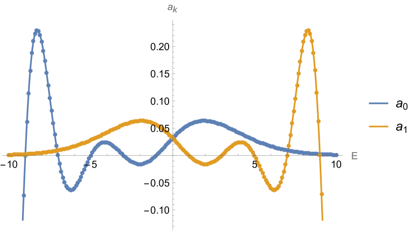
Figure 1: The prefactors of the two types of asymptotic behaviors in (16) at various $E$. The bounded-from-above energy spectrum is associated with the zeros of $a_{1}[E]$. The dots are obtained numerically by matching the non-perturbative solutions for $G_{n}$ with the $1/n$ series (16). The curves are from the analytic expression for $a_{0}$ in (28) and the relation between $a_{0}$ and $a_{1}$ in (22). The numerical values are interpolated by the analytic formulae.

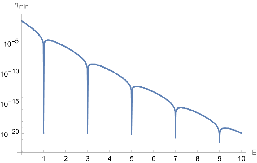
Figure 2: The $\eta_{\text{min}}$ landscape of the quantum harmonic oscillator. The local minima are consistent with the exact spectrum in (10).

Let us use the quantization condition (23) to deduce the energy spectrum. We impose that the finite $n$ solutions for $G_{n}$ at relatively large $n$ matches with the $1/n$ expansion of $G_{n}$. Since $a_{1}=0$, there remain two free parameters, i.e., $(E,a_{0})$, which can be determined by the two matching conditions

$$G_{M}^{(\text{n.p.})}=G_{M}^{(\text{p.})}\,,\quad G_{M+2}^{(\text{n.p.})}=G_{M+2}^{(\text{p.})}\,.$$ (24)

Note that $M$ denotes the matching order, $G_{n}^{(\text{n.p.})}$ indicates the non-perturbative finite $n$ expressions of $G_{n}$ from the recursion relation (9), and $G_{n}^{(\text{p.})}$ is given by the perturbative $1/n$ series in (16). As $(M,N)$ increase, it requires some efforts to deduce all the solutions of the matching conditions (24) due to the nonlinear $E$ dependence. Since we are mainly interested in the positive real energy solutions, we can reformulate the difficult problem of solving highly nonlinear equations as the simpler least-square problem. To measure the errors in the matching conditions (24), we introduce the $\eta$ function

$$\eta=\sqrt{\sum_{n}\left(G_{n}^{(\text{n.p.})}-G_{n}^{(\text{p.})}\right)^{2}}\,.$$ (25)

It is useful to divide $G_{n}$ by the leading asymptotic behavior so that each term is of order $\mathcal{O}(1)$. As $G_{n}^{(\text{p.})}$ is linear in $a_{0}$, it is straightforward to minimize the $\eta$ function for a given $E$. We can scan the $\eta_{\text{min}}$ landscape as a function of $E$. The solutions of the matching conditions (24) are associated with the local minima with $\eta_{\text{min}}=0$. In Fig. 2, we present the $\eta_{\text{min}}$ landscape for $(M,N)=(100,10)$, which contains 5 local minima with $\eta_{\text{min}}=0$ in the range $0<E<10$. All of them can be identified with the exact values from (10):

$$E^{(k=0)}_{\text{approx.}}-1\approx 3\times 10^{-17}\,,\quad E^{(k=1)}_{\text{approx.}}-3\approx-3\times 10^{-13}\,,\quad E^{(k=2)}_{\text{approx.}}-5\approx 8\times 10^{-10}\,,$$

$$E^{(k=3)}_{\text{approx.}}-7\approx-8\times 10^{-7}\,,\quad E^{(k=4)}_{\text{approx.}}-9\approx 3\times 10^{-4}\,,$$ (26)

where the errors grow with $k$. There are more local minima at larger $E$. The solutions for $a_{1}$ are approximately given by

$$4\sqrt{2}\,\pi\,\Gamma\left(\frac{1+E}{2}\right)a_{0}-1\approx 1\times 10^{-18}\,,$$ (27)

which indicates the analytic expression

$$a_{0}[E]=\frac{1}{4\sqrt{2}\,\pi}\frac{1}{\Gamma\left(\frac{1+E}{2}\right)}\,.$$ (28)

As $(M,N)$ increase, the numerical solutions converge rapidly to the analytic values in (10) and (28). According to (22) and (28), the explicit expression of the quantization condition (23) reads

$$a_{1}(E)=\frac{1}{4\sqrt{2}\,\pi}\frac{1}{\Gamma\left(\frac{1-E}{2}\right)}=0\,.$$ (29)

The solutions are identical to the exact values in (10).

Let us make some consistency checks. When $E$ takes an exact value in (10), we verify that the corresponding $1/n$ series is compatible with the minimally singular form, i.e., (16) with $a_{1}=0$. For notational simplicity, we will not write the factor $\frac{1+(-1)^{n}}{2}$ explicitly. Some examples are

$$G^{(E=1)}_{n} = \left(\frac{1}{2}\right)_{n/2}\sim 2^{n/2}\left[\Gamma\left(\frac{n}{4}\right)\right]^{2}n^{1}\frac{1-\frac{3}{4n}+\frac{9}{32n^{2}}+\frac{39}{128n^{3}}+\dots}{4\sqrt{2}\,\pi\,\Gamma(1)}\,,$$ (30)

$$G^{(E=3)}_{n} = \left(\frac{3}{2}\right)_{n/2}\sim 2^{n/2}\left[\Gamma\left(\frac{n}{4}\right)\right]^{2}n^{2}\frac{1+\frac{1}{4n}-\frac{15}{32n^{2}}+\frac{75}{128n^{3}}+\dots}{4\sqrt{2}\,\pi\,\Gamma(2)}\,,$$ (31)

$$G^{(E=5)}_{n} = \frac{n^{2}+2n+2}{2}\left(\frac{1}{2}\right)_{n/2}\sim 2^{n/2}\left[\Gamma\left(\frac{n}{4}\right)\right]^{2}{n^{3}}\frac{1+\frac{5}{4n}+\frac{25}{32n^{2}}-\frac{81}{128n^{3}}+\dots}{4\sqrt{2}\,\pi\,\Gamma(3)}\,,\quad$$ (32)

$$G^{(E=7)}_{n} = \frac{n^{2}+2n+6}{6}\left(\frac{3}{2}\right)_{n/2}\sim 2^{n/2}\left[\Gamma\left(\frac{n}{4}\right)\right]^{2}{n^{4}}\frac{1+\frac{9}{4n}+\frac{193}{32n^{2}}+\frac{147}{128n^{3}}+\dots}{4\sqrt{2}\,\pi\,\Gamma(4)}\,,\quad$$ (33)

where $\dots$ indicates higher order terms in the $1/n$ expansion. The concrete values of $a_{0}$ are also consistent with the analytic expression (28). If $E$ is not a positive odd integer, the large $n$ expansion should involve a nonzero $a_{1}$. In the simple case of $E=0$, the recursion relation (9) can be solved explicitly

$$G^{(E=0)}_{n} = \frac{(1+(-1)^{n/2})\Gamma(\frac{n+1}{2})\Gamma(\frac{n+2}{4})}{2\pi\Gamma(\frac{n+4}{4})}\sim 2^{n/2}\left[\Gamma\left(\frac{n}{4}\right)\right]^{2}\,{n^{\frac{1}{2}}}\frac{1+(-1)^{n/2}+\dots}{4\sqrt{2}\pi\,\Gamma(1/2)}\,.\quad$$ (34)

Therefore, we have $a_{1}=a_{0}$ as expected from the $E\rightarrow-E$ symmetry. The exact value of $a_{0}$ at $E=0$ also confirms the analytic expression in (28).

As we have deduced the complete energy spectrum, it is interesting to examine the large $E$ asymptotic behavior. For small $n$, the Green’s functions can be approximated by

$$G_{n}\sim E^{\frac{n}{2}}\frac{(1/2)_{n/2}}{(1)_{n/2}}\left(1+\frac{(n-2)_{3}}{24E^{2}}+\dots\right)\quad(E\rightarrow\infty)\,.$$ (35)

We can also consider the large $n$ region. The prefactor of the $1/n$ series is given by

$$a_{0}[E]\sim\frac{(2e)^{E/2}E^{-E/2}}{8\pi^{3/2}}\left(1+\frac{1}{12E}+\frac{1}{288E^{2}}+\dots\right)\quad(E\rightarrow\infty)\,.$$ (36)

The vanishing condition (29) for the other prefactor becomes

$$a_{1}[E]\sim\frac{(2e)^{-E/2}E^{E/2}}{4\pi^{3/2}}\cos\Big{(}\frac{\pi}{2}\,E\Big{)}\left(1-\frac{1}{12E}+\frac{1}{288E^{2}}+\dots\right)=0\quad(E\rightarrow\infty)\,,$$ (37)

which also gives the exact spectrum (10) due to the exact form of the oscillatory part $\cos\big{(}\frac{\pi}{2}\,E\big{)}$. In analogy with the WKB method, one should be able to derive the asymptotic quantization condition (37) directly from the global asymptotic solution for $G_{n}$ at large $E$.

It is interesting to consider the composite operators involving $p$ or time derivatives. A simple example for multiple $p$ is

$$\left\langle p^{n}\right\rangle=\left\langle\phi^{n}\right\rangle\,,$$ (38)

as the harmonic oscillator Hamiltonian is symmetric in $p$ and $\phi$. A simple example for multiple time derivatives is

$$\left\langle\phi\frac{d\phi^{n}}{d\tau^{n}}\right\rangle=\partial_{\tau_{2}}^{n}\,G_{2}(\tau_{1},\tau_{2})\big{|}_{\tau_{2}\rightarrow\tau_{1}}=\frac{E^{n+1}}{2}\,,$$ (39)

where $\tau_{1},\,\tau_{2}$ are the Euclidean time coordinates for the 2-point Green’s function $G_{2}$ and we assume $\tau_{1}\geq\tau_{2}$. For simplicity, we assume that $n$ is a positive integer. A proper analytic continuation to complex $n$ requires some care.

Below we show that the bootstrap analysis in this section can be applied to the anharmonic oscillators that do not admit simple analytic solutions.

3 $V(\phi)=\phi^{2}+\phi^{m}$

In this section, we consider the Hermitian anharmonic oscillator

$$H=p^{2}+\phi^{2}+\phi^{m}\,,$$ (41)

where we assume that $m\geq 4$ and $m$ is an even integer. The Hamiltonian (41) is invariant under the parity transformation

$$\phi\rightarrow-\phi\,.$$ (42)

The recursion relation (7) reads

$$(n+1)_{3}G_{n}+4E(n+3)G_{n+2}=4(n+4)G_{n+4}+2(2n+m+6)G_{n+m+2}\,,$$ (43)

where the Green’s functions $G_{n}$ are defined as the expectation values

$$G_{n}=\left\langle\phi^{n}\right\rangle\,.$$ (44)

The normalization is fixed by $G_{0}=1$. For parity symmetric solutions, $G_{n}$ vanishes if $n$ is an odd integer. For $G_{n}$ with integer $n>0$, there are $m/2$ free parameters. We choose the independent set of free parameters as

$$(E\,,G_{2}\,,G_{4}\,,\dots,G_{m-2})\,.$$ (45)

The other $G_{n}$ at integer $n$ can be determined by the recursion relation (43). As $n$ increases, the analytic expressions of the nonperturbative solutions for $G_{n}$ are of high degree in $E$, but at most linear in $(G_{2}\,,G_{4}\,,\dots,G_{m-2})$.

3.1 $m=4$

For the quartic oscillator $m=4$, the Hamiltonian reads

$$H=p^{2}+x^{2}+x^{4}\,.$$ (46)

There are only two free parameters

$$(E,\,G_{2})\,.$$ (47)

The large $n$ expansion of the correct solution reads

$$G_{n}\sim a_{0}\frac{1+e^{2\pi i\frac{n}{2}}}{2}3^{n/3}n^{1/6}\left[\Gamma\left(\frac{n}{6}\right)\right]^{2}e^{-\left(\frac{n}{2}\right)^{1/3}}\left(1+\sum_{k=1}^{3N}c_{k}\left(\frac{n}{2}\right)^{-k/3}\right)\quad(n\rightarrow\infty)\,,\quad$$ (48)

where $N$ is the truncation order of the $1/n$ series. The explicit expressions of some low order coefficients are

$$c_{1}=-E-\frac{1}{6}\,,\quad c_{2}=\frac{36E^{2}+12E-11}{72}\,,\quad c_{3}=\frac{-216E^{3}-108E^{2}+198E-883}{1296}\,.$$ (49)

The free parameters can be determined to high accuracy by the matching procedure. The ground state solution corresponds to

$$a_{0} = 0.484173090557323742122230381577...\,,$$ (50)

$$E = 1.39235164153029185565750787661...\,,$$ (51)

$$G_{2} = 0.305813650717587136934033799352...\,,$$ (52)

which can be obtained from the matching conditions with $(M,N)=(200,20)$.

Alternatively, we can study $G_{n}=\left\langle\phi^{n}\right\rangle$ in the standard wave function formulation. In terms of the harmonic oscillator eigenfunctions, the matrix elements of the Hamiltonian (46) can be computed analytically. The diagonalization of a truncated Hamiltonian can give accurate approximations for the energy eigenvalues and eigenfunctions. We can use the approximate wave function $\psi[\phi]$ to compute $G_{n}$ based on the standard Hermitian inner product

$$G_{n}=\left\langle\phi^{n}\right\rangle=\int_{-\infty}^{\infty}d\phi\,\psi^{\ast}[\phi]\,\phi^{n}\,\psi[\phi]\,.$$ (53)

The ground state estimates agree well with the matching results (51) and (52).

It is usually assumed that $n$ is a positive integer, but there is no obstruction to evaluate the integral in (53) for complex $n$. In Fig. 3, we compare the results from the wave function formulation and the minimally singular solution (48) with (50), (51). We find perfect agreement for both real and complex $n$. In Fig. 4, we present the real and imaginary parts of $G_{n}$ as a function of complex $n$.

For relatively large $\text{Re}(n)$, the minimally singular solution can evaluated directly using the $1/n$ series (48). However, the direct evaluation at small $\text{Re}(n)$ is not accurate due to the asymptotic nature of the large $n$ expansion. To resolve this issue, we use the recursion relation (43) to express $G_{n}$ at small $\text{Re}(n)$ in terms of $G_{n}$ at relatively large $\text{Re}(n)$. In this way, we can evaluate the minimally singular solution accurately at small $\text{Re}(n)$ as well. This is also the basic idea behind the matching procedure.

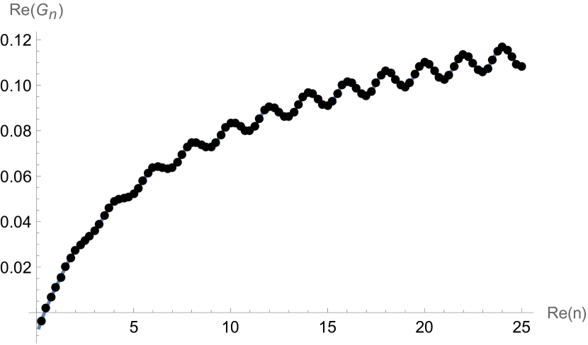
(a) $\text{Re}(G_{n})$ with $\text{Im}(n)=1$

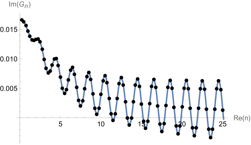
(b) $\text{Im}(G_{n})$ with $\text{Im}(n)=1$

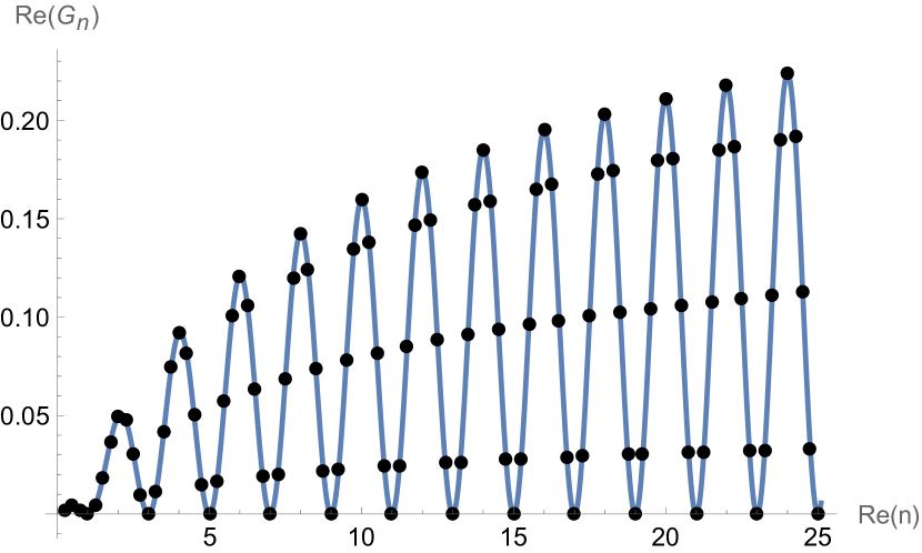
(c) $\text{Re}(G_{n})$ with $\text{Im}(n)=0$

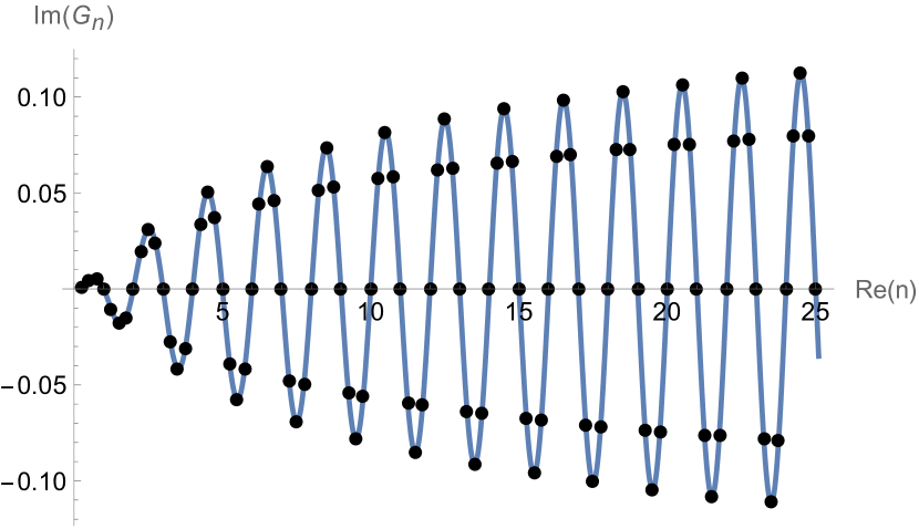
(d) $\text{Im}(G_{n})$ with $\text{Im}(n)=0$

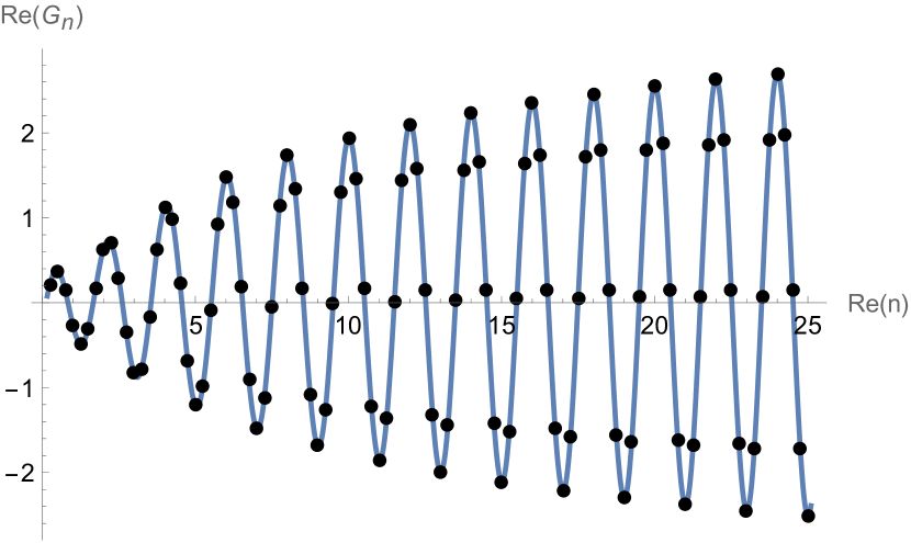
(e) $\text{Re}(G_{n})$ with $\text{Im}(n)=-1$

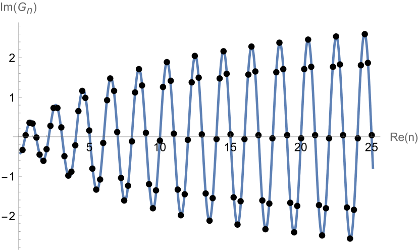
(f) $\text{Im}(G_{n})$ with $\text{Im}(n)=-1$

Figure 3: The Green’s functions $G_{n}=\left\langle\phi^{n}\right\rangle$ of the Hermitian quartic oscillator (46) as a function of the real part of $n$. The imaginary part of $n$ is fixed to be $\text{Im}(n)=-1,0,1$. The values of the black dots at $\text{Re}(n)=p/4$ are computed using the standard Hermitian inner product (53) and the ground-state wavefunction from the Hamiltonian diagonalization. The blue curves are associated with the minimally singular solution (48) with (50), (51). The black dots are well interpolated by the blue curves.

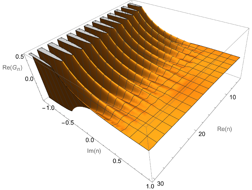
(a) $\text{Re}(G_{n})$

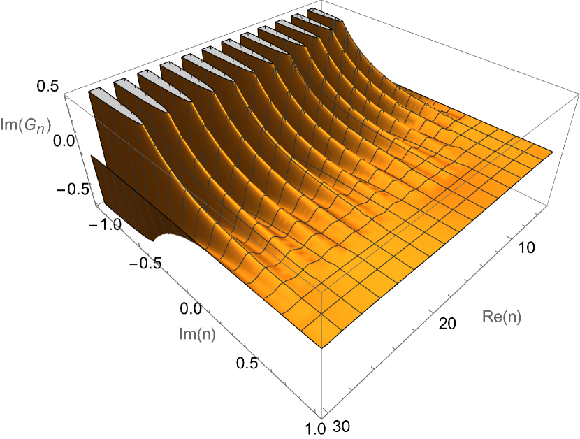
(b) $\text{Im}(G_{n})$

Figure 4: The ground state Green’s function $G_{n}=\left\langle\phi^{n}\right\rangle$ of the Hermitian quartic oscillator (46) as a function of complex $n$. They are computed by the large $n$ expansion of the minimally singular solution (48) with (50), (51). The $1/n$ series is truncated to order $n^{-5}$.

3.2 Higher even powers

Let us consider the cases with higher power $m$. Although the number of free parameters grows with $m$, we still obtain highly accurate results using the matching procedure. At large $n$, the leading behavior is determined by the leading terms in (43):

$$n^{3}G_{n}\sim 4nG_{n+m+2}\quad(n\rightarrow\infty)\,.$$ (54)

The general form of the leading asymptotic behavior is given by

$$G_{n}\sim\left(\frac{m}{2}+1\right)^{\frac{2n}{m+2}}\,\left[\Gamma\left(\frac{n}{m+2}\right)\right]^{2}\,\sum_{k=0}^{m+1}\,a_{k}\,e^{2\pi i\frac{kn}{m+2}}\quad(n\rightarrow\infty)\,.$$ (55)

The parity symmetry implies the constraints $a_{k}=a_{k+m/2+1}$. As in the quartic case, the correct solution is the minimally singular solution with $a_{0}=a_{m/2+1}\neq 0$. If we take into account the subleading terms in (43), there exists an additional factor, whose general form is $n^{-\frac{m-6}{2(m+2)}}$. For $m\geq 8$, the large $n$ expansion reads

$$G_{n} \sim a_{0}\frac{1+e^{2\pi i\frac{n}{2}}}{2}\left(\frac{m}{2}+1\right)^{\frac{2n}{m+2}}\,\left[\Gamma\left(\frac{n}{m+2}\right)\right]^{2}n^{-\frac{m-6}{2(m+2)}}\left(1+\sum_{j=m/2-3}^{(m/2+1)N}\,c_{j}\left(\frac{n}{2}\right)^{-\frac{2j}{m+2}}\right)\,,$$

where the $1/n$ series is truncated to order $n^{-N}$. The series coefficients can be computed order by order. If $m$ is an odd integer, the coefficients $c_{j}$ vanish for odd $j$. For large $m$, the low order coefficients take some general forms. For example, the low order nonzero coefficients for $m\geq 16$ are

$$c_{m/2-3}=\frac{2}{m-6}\,,\quad c_{m/2-1}=-\frac{2E}{m-2}\,,\quad c_{m/2+1}=\frac{m^{2}-20m-4}{16(m+2)}\,.$$ (57)

In fact, the expression of $c_{m/2-1}$ applies to $m\geq 12$, while that of $c_{m/2-3}$ is valid for $m\geq 8$. As $m$ decreases, the $1/n$ expansion of the recursion relation can have degenerate exponents at low order, so the concrete expressions of $c_{j}$ can be different from the general forms in (57). For $m=6$, the additional factor $n^{-1/4}$ is different from the generic form due to the degeneracy in the exponents of the $1/n$ expansion. For $m=4$, the large $n$ expansion in (48) has two additional factors, i.e. an expected factor $n^{1/6}$ and a special factor $e^{-(n/2)^{1/3}}$.

As in the harmonic example, the free parameters in (45) and $a_{0}$ can be determined by the matching conditions

$$G_{n}^{(\text{n.p.})}=G_{n}^{(\text{p.})}\,,\quad n=M,M+2,\dots,M+m\,,$$ (58)

where $M$ indicates the matching order, $G_{n}^{(\text{n.p.})}$ is the non-perturbative solutions for $G_{n}$ of from (43), and $G_{n}^{(\text{p.})}$ is given by the $1/n$ series in (LABEL:large-n-expansion-x-2m). The number of matching constraints grows with $m$ as there are more free parameters. They lead to polynomial equations in the free parameters.

As $m$ increases, it becomes more and more challenging to solve a large set of high degree polynomial equations with multiple variables. Note that these equations are linear in $G_{2},\dots,G_{m-2}$ and $a_{0}$. Only the $E$ dependence is nonlinear. For Hermitian solutions, the energy should be real and the complex solutions are irrelevant. As in the case of the harmonic oscillator, we introduce the $\eta$ function (25) and transform the difficult problem of solving a large set of high degree polynomial equations into an easier minimization problem. After deriving the explicit expressions of $G_{n}^{(\text{n.p.})}$ and $G_{n}^{(\text{p.})}$, we scan the real $E$ and search for the local minima of $\eta$ with $\eta_{\text{min}}=0$, which leads to highly accurate results for the energies and expectation values.

In Fig. 5, we compare the errors in the ground state energy $E_{0}$ from the matching approach and the Hamiltonian diagonalization approach for $m=6,8,\dots,16$. As $m$ increases, the accuracy of the diagonalization results decreases rapidly, but the matching conditions still lead to highly accurate results for the same set of truncation orders $(M,N)$. The matching procedure seems to be more efficient, especially at larger $m$.

As we do not use any positivity constraints, the matching procedure also applies to the non-Hermitian models, which can violate some positivity assumptions. Below, we extend the discussion to the non-Hermitian $\mathcal{PT}$ invariant oscillators.

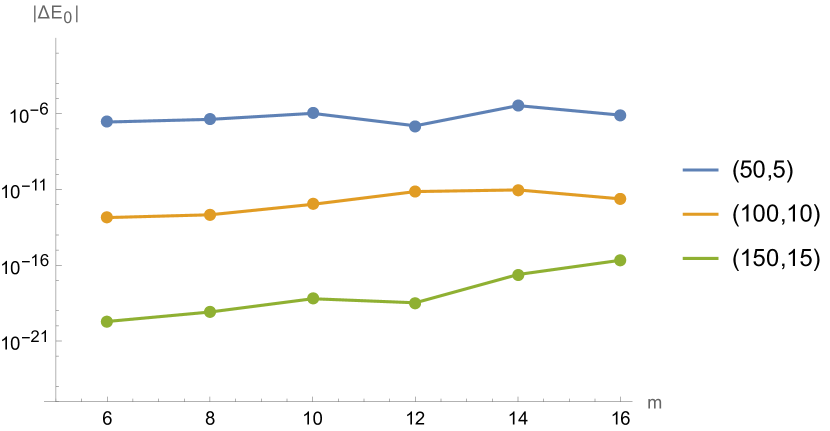
(a) Matching $G_{n}$ with different $(M,N)$.

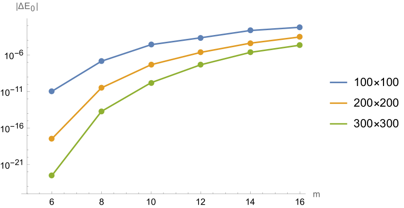
(b) Diagonalizing $H$ with different sizes.

Figure 5: The absolute errors in the ground state energy $E_{0}$ for $H=p^{2}+\phi^{2}+\phi^{m}$ from (a) the matching procedure and (b) the Hamiltonian diagonalization. The matching conditions (58) are evaluated at $n=M,M+2,\dots,M+m$, while the $1/n$ series (LABEL:large-n-expansion-x-2m) is truncated to order $n^{-N}$. The matrix elements of the truncated Hamiltonian are computed in the truncated bases of the harmonic oscillator eigenfunctions, which contain $100k$ low-lying eigenfunctions with $k=1,2,3$. As $m$ increases, the accuracy of the diagonalization approach decreases significantly, but the matching approach still gives highly accurate results.

4 $V(\phi)=-(i\phi)^{m}$

In this section, we consider the non-Hermitian Hamiltonian

$$H=p^{2}-(i\phi)^{m}\,,$$ (59)

which is invariant under the $\mathcal{PT}$ transformation

$$\phi\rightarrow-\phi\,,\quad i\rightarrow-i\,.$$ (60)

In accordance with $\mathcal{PT}$ symmetry, we define the Green’s functions as

$$G_{n}=\left\langle(i\phi)^{n}\right\rangle\,.$$ (61)

Note that $i\phi$ plays an analogous role as $\phi^{2}$ in the parity invariant cases, but there is no simple vanishing constraints on $G_{n}$ associated with $\mathcal{PT}$ symmetry. The recursion relation (7) becomes

$$(n+1)_{3}G_{n}-4E(n+3)G_{n+2}=2(2n+m+6)G_{n+m+2}\,,$$ (62)

where the normalization is set by $G_{0}=1$.

4.1 Integral powers

Let us assume that $m\geq 3$ and $m$ is an integer. The independent set of free parameters is chosen to be

$$(E\,,G_{1}\,,G_{2}\,,\dots,G_{m-2})\,.$$ (63)

The leading asymptotic behavior can be derived from

$$n^{3}G_{n}\sim 4n\,G_{n+m+2}\quad(n\rightarrow\infty),$$ (64)

so the general leading behavior takes the same form as (55):

$$G_{n}\sim\left(\frac{m}{2}+1\right)^{\frac{2n}{m+2}}\,\left[\Gamma\left(\frac{n}{m+2}\right)\right]^{2}\,\sum_{k=0}^{m+1}\,a_{k}\,e^{2\pi i\frac{kn}{m+2}}\quad(n\rightarrow\infty)\,.$$ (65)

After taking into account the subleading terms, we obtain the $1/n$ series

$$G_{n} \sim \left(\frac{m}{2}+1\right)^{\frac{2n}{m+2}}\left[\Gamma\left(\frac{n}{m+2}\right)\right]^{2}n^{-\frac{m-6}{2(m+2)}}\sum_{k=0}^{m+1}a_{k}\,e^{2\pi i\frac{kn}{m+2}}\left(1+\sum_{j=m-2}^{(m+2)N}c_{k,j}\left(\frac{n}{2}\right)^{-\frac{j}{m+2}}\right)\,,$$ (66)

$$\quad(n\rightarrow\infty)\,,$$

which is truncated to order $n^{-N}$. The coefficients $c_{k,j}=c_{k,j}(E)$ are functions of the energy $E$. Since the recursion relation (62) is invariant under the rotation

$$G_{n}\rightarrow G_{n}\,e^{2\pi i\frac{kn}{m+2}}\,,\quad E\rightarrow E\,e^{2\pi i\frac{(-2)k}{m+2}}\,,$$ (67)

the $k\neq 0$ series coefficients are related to $c_{0,j}$ by

$$c_{k,j}(E)=c_{0,j}\big{(}Ee^{2\pi i\frac{2k}{m+2}}\big{)}\,,$$ (68)

which generalizes the relation (21) in the harmonic case $m=2$. For odd $m$, we also notice that $c_{k,j}(E)=c_{0,j}(E)\,e^{2\pi i\frac{(m+1)k}{2(m+2)}}$. At large $m$, the low order coefficients take the general forms

$$c_{0,m-2}=\frac{2E}{m-2}\,,\quad c_{0,m+2}=\frac{m^{2}-20m-4}{16(m+2)}\,,$$ (69)

$$c_{0,2m-4}=\frac{2E^{2}}{(m-2)^{2}}\,,\quad c_{0,2m}=\frac{(5m^{2}-44m+28)E}{8(m^{2}-4)}\,.$$ (70)

The $\mathcal{PT}$ symmetry implies that $G_{n}=\left\langle(i\phi)^{n}\right\rangle$ should be real for real $n$, so we have

$$a_{m+2-k}=(a_{k})^{\ast}\,.$$ (71)

It turns out that the $\mathcal{PT}$ symmetric solutions have only two nonvanishing $a_{1}$ and $a_{m+1}$, so they also belong to the minimally singular solutions. To determine the free parameters, we impose the matching conditions

$$G_{n}^{(\text{n.p.})}=G_{n}^{(\text{p.})}\,,\quad n=M,M+1,\dots,M+m\,.$$ (72)

As before, $G_{n}^{(\text{n.p.})}$ are obtained by solving the recursion relation (62). Their analytic expressions are at most linear in $(G_{1}\,,G_{2}\,,\dots,G_{m-2})$, but they can be of high degree in $E$. We again introduce the $\eta$ function (25). The solutions to the matching conditions (72) correspond to the local minima with $\text{min}(\eta)=0$. In Fig. 6(a), we present the results for the ground state energy $E_{0}$ at various integer $m$. In Fig. 7(a), we show that the absolute error in $E_{0}$ only grows mildly as $m$ increases.

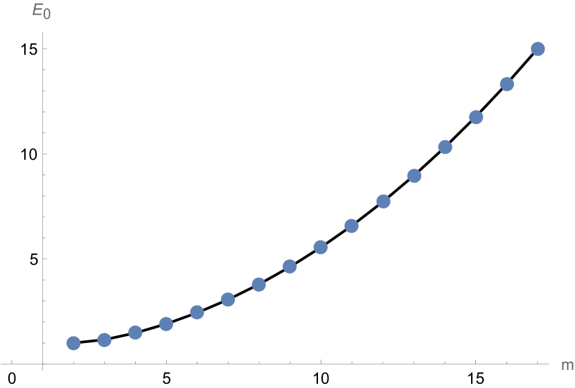
(a) $2\leq m\leq 17$

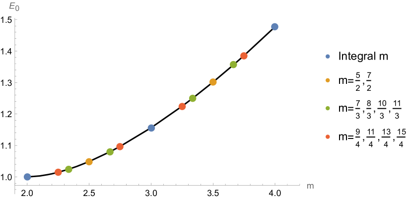
(b) $2\leq m\leq 4$

Figure 6: The ground state energy $E_{0}$ of the non-Hermitian Hamiltonian $H=p^{2}-(i\phi)^{m}$ at various $m$. We focus on the $\mathcal{PT}$ symmetric cases. In (a), we present the integral $m$ results for $2\leq m\leq 17$. In (b), we zoom in on the range $2\leq m\leq 4$ and present some fractional $m$ results as well.

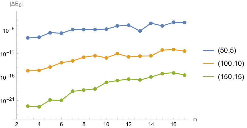
(a) $m=3,4,\dots,17$

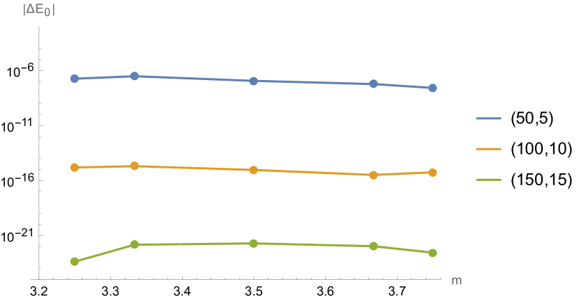
(b) $m=\frac{13}{4},\frac{10}{3},\frac{7}{2},\frac{11}{3},\frac{15}{4}$

Figure 7: Absolute errors in the ground state energies of $H=p^{2}-(i\phi)^{m}$ at various $m$ with $(M,N)=(50,5),(100,10),(150,15)$. We use $M$ to denote the matching order and $N$ to indicate the truncation order of the $1/n$ series. We present the integral $m$ results for $3\leq m\leq 17$. Then we zoom in on the range $3\leq m\leq 4$ and present the results at some fractional $m$.

According to the accurate solutions from the matching procedure, we notice that the argument of $a_{1}$ takes a simple analytic form

$$\arg[a_{1}]=\frac{m+10}{2(m+2)}\pi\,,$$ (73)

which should be related to the choice of the Stokes sectors. Note that $\arg[a_{1}]$ vanishes at $m=6$. The deviation of the numerical solution for $\arg[a_{1}]$ from the analytic prediction (73) also provides an error estimation for the matching results.

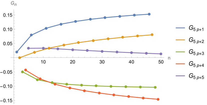
(a) $n=1,2,\dots,50$

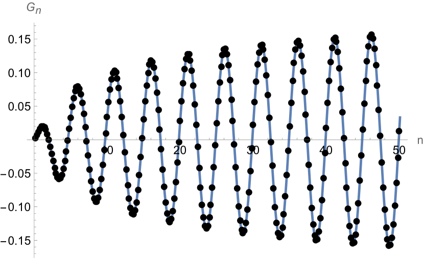
(b) $n=\frac{1}{5},\frac{2}{5},\dots,\frac{249}{5},\frac{250}{5}$

Figure 8: The ground state Green’s functions $G_{n}=\left\langle(i\phi)^{n}\right\rangle$ of the non-Hermitian cubic theory $H=p^{2}-(i\phi)^{3}$. According to the integral $n$ results from the Hamiltonian diagonalization, one may naively find 5 branches of Green’s functions, as indicated in (a) . However, as we also present the fractional $n$ results in (b),, an oscillatory curve emerges. This is precisely the minimally singular solution with (75) and (76) (blue curve).

Before considering the cases with fractional power $m$, let us revisit the basic example of the cubic oscillator, i.e., $m=3$. If we focus on $G_{n}$ with integer $n$, there seem to be 5 branches of Green’s functions, corresponding to $G_{5p+k}$ with $k=1,2,3,4,5$, as shown in Fig. 8(a). However, the analytic continuation in $n$ allows us to consider $G_{n}$ at non-integer $n$. One may wonder if they correspond to more exotic branches of solutions.

As in the Hermitian cases in Sec. 3, we can also study the non-Hermitian $G_{n}$ using the wave function formulation. According to the symmetry of the Hamiltonian (59), it is natural to use the $\mathcal{PT}$ inner product

$$G_{n}=\left\langle(i\phi)^{n}\right\rangle=\int_{-\infty}^{\infty}d\phi\,\{\psi[-\phi]\}^{\ast}\,(i\phi)^{n}\,\psi[\phi]\,,$$ (74)

which is valid for $1<m<4$. We assume that the wave function $\psi[\phi]$ is $\mathcal{PT}$ symmetric. In Fig. 8(b), we present the ground-state results from the wave function formulation at fractional $n=p/5$, where $p$ is a positive integer. It is clear that they are interpolated by an oscillatory curve, which is similar the quartic case in Fig. 3. The interpolating function is precisely the minimally singular solution associated with the $\mathcal{PT}$ invariant ground state:

$$a_{1} = -0.128537084089570612897940053524...$$ (75)

$$-0.176916118650967924857364104948...i\,,$$

$$E = 1.15626707198811329379921917800...\,,$$ (76)

$$G_{1} = 0.590072533090700847855025174549...\,,$$ (77)

where the argument of $a_{1}$ is consistent with the analytic expression (73). Therefore, the 5 naively different branches of Green’s functions at integer $n$ are unified by the oscillatory minimally singular solution. There is only one interpolating solution for both the integer and non-integer $n$. For small $\text{Re}(n)$, we again use the recursion relation to obtain accurate results for $G_{n}$.

4.2 Fractional powers

In the Hermitian quartic and non-Hermitian cubic cases, we verify that the minimally singular solution for $G_{n}$ at non-integer $n$ is consistent with the results from the more standard wave function formulation, so the $n$ complexification is not a purely mathematical trick. In fact, if we want to bootstrap the cases with non-integer power $m$, it is inevitable to consider $G_{n}$ with non-integer $n$, which was one of the main motivations for studying the analytical continuation in $n$ Li:2022prn .

For simplicity, we will focus on the cases of fractional $m$, but the general procedure can be extended to irrational $m$ as well. In order to compare with the results from the wave function formulation, we restrict the range of $m$ to $2<m<4$ where the standard diagonalization method is valid. In Fig. 6(b), we present some results for the ground state energy at fractional $m$, which leads to a smooth interpolating curve. In Fig. 7(b), we show that the matching results remain highly accurate for fractional $m$, as in the integer $n$ cases.

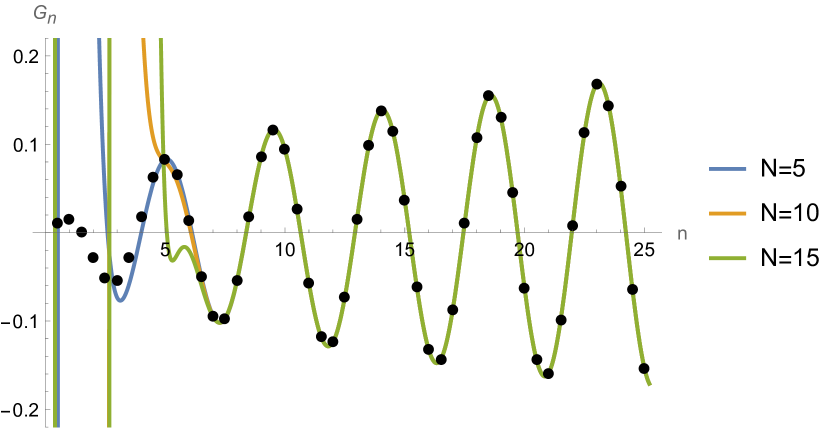
(a) $m=\frac{5}{2},\,n=\frac{p}{2}$

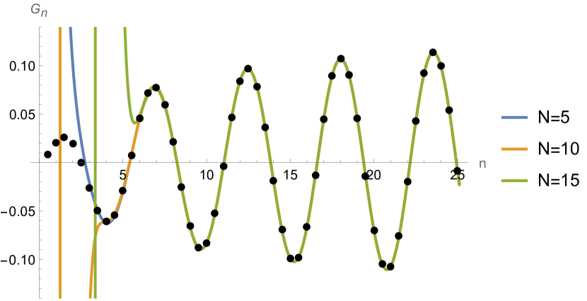
(b) $m=\frac{7}{2},\,n=\frac{p}{2}$

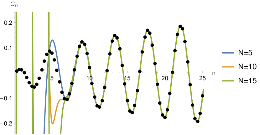
(c) $m=\frac{7}{3},\,n=\frac{p}{3}$

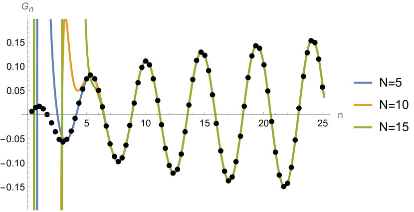
(d) $m=\frac{8}{3},\,n=\frac{p}{3}$

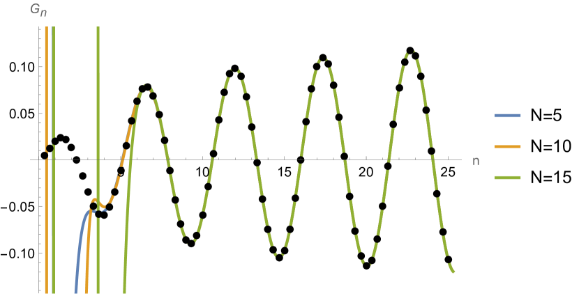
(e) $m=\frac{10}{3},\,n=\frac{p}{3}$

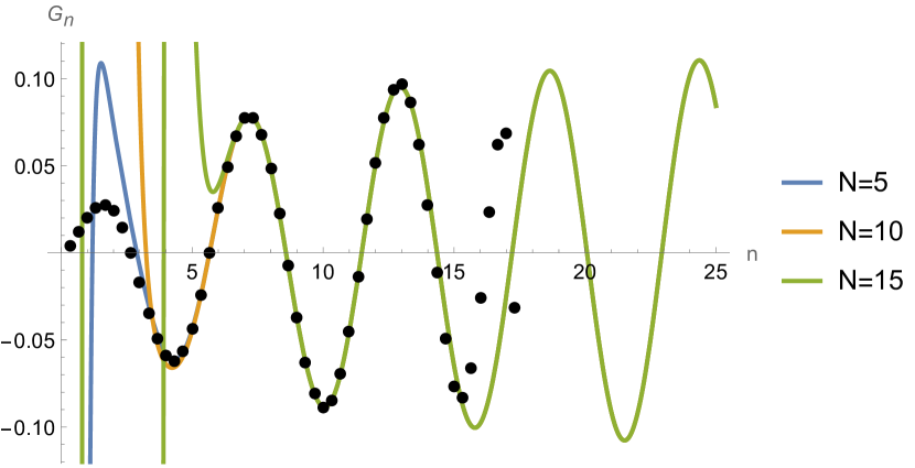
(f) $m=\frac{11}{3},\,n=\frac{p}{3}$

Figure 9: Comparison between the asymptotic $1/n$ expansion and the wave function results for $G_{n}=\left\langle(i\phi)^{n}\right\rangle$. We focus on the $\mathcal{PT}$ symmetric ground states of the non-Hermitian Hamiltonian $H=p^{2}-(i\phi)^{m}$. For the minimally singular solutions, the truncation order of the $1/n$ series is given by $N=5,10,15$. We consider several fractional $m$ examples in the range $2<m<4$, which can be studied by the standard method of diagonalizing the truncated Hamiltonian of size $250\times 250$. We use the approximate ground-state wavefunction to compute $G_{n}$ at various $n$, which are labelled by the integer parameter $p$. The large $n$ series results match well with the diagonalization results for sufficiently large $n$. On the other hand, if $n$ is too large, the diagonalization results would have noticeable errors. In the $m=11/3$ case, the diagonalization results have significant errors for $n>14$ due to the slow convergence of the diagonalization method near $m=4$.

In Fig. 9, we present the Green’s functions at various real $n$ for $m=\frac{5}{2},\frac{7}{2}$ and $m=\frac{7}{3},\frac{8}{3},\frac{10}{3},\frac{11}{3}$. The results from the ground state wave functions are again in perfect agreement with the minimally singular solutions with $a_{1}=(a_{m+1})^{\ast}\neq 0$. To show the asymptotic nature of the large $n$ expansion, we present the results associated with the truncated $1/n$ series of order $n^{-5},n^{-10},n^{-15}$. We do not use the recursion relation (62) to improve the low $n$ results as in the cubic and quartic examples above. As expected, a higher order $1/n$ series gives more accurate estimates at large $n$, but the asymptotic series becomes less reliable at small $n$ as the truncation order $N$ increases.

In some sense, a fractional $m$ case can be viewed as a multi-covering version of an integral $m$ case. The number of covering is associated with the denominator of $m$, while the length of a complete period is related to the numerator of $m+2$. If $m=p_{1}/p_{2}$ is and $(p_{1},p_{2})$ are integers with no common divisor, then the total number of free parameters is $p_{1}+2p_{2}-1$. The general form of the large $n$ expansion is similar to the integral $m$ case (66), but the spacing of $j$ is reduced to $1/p_{2}$. The matching procedure is the same as before. The analytic expression for $\arg[a_{1}]$ in (73) also applies to the fractional $m$ cases.

5 Discussion

In this work, we have further investigated the bootstrap approach based on the analytic continuation of the Green’s functions $G_{n}$ to complex $n$. We used the harmonic oscillator to illustrate various aspects of the bootstrap analysis both numerically and analytically, including the large $n$ expansion of self-consistent solutions, the matching between the perturbative $1/n$ series and the non-perturbative finite $n$ solutions, the principle of minimally singularity as an exact quantization condition, and the high energy asymptotic behavior of the Green’s functions. The two questions raised in the introduction have been addressed:

1. The Green’s functions $G_{n}$ at non-integer $n$ are consistent with the results from the standard wave function formulation.

2. The matching procedure for $G_{n}$ gives highly accurate results for the anharmonic potential with higher powers and non-integer powers.

For $D=0$, the basic physical observables are associated with composite operators $\phi^{n}$. It is natural to consider the analytic continuation in the number of the fundamental field. For $D>1$, we can construct composite operators using both fundamental fields and derivatives, so it is natural to complexify the numbers of derivatives as well. In the Hamiltonian formulation, we can consider both the fundamental fields and their canonical conjugates. It is also interesting to go beyond the one-point functions of composite operators. For applications to particle physics and condensed matter physics, it is important to introduce the fermionic degrees of freedom. We can analytically continue the numbers of bilinear operators, such as $(\bar{\psi}\psi)^{n}$.

It would be fascinating to further explore the various possibilities on the interplay between self-consistency and analyticity. Our hope is that this will lead to efficient non-perturbative methods for studying the strongly coupled and strongly correlated physics in realistic quantum field theories and quantum many body systems.

References

- (1) T. Regge, “Introduction to complex orbital momenta,” Nuovo Cim. 14, 951 (1959) doi:10.1007/BF02728177
- (2) G. F. Chew, “The S-matrix theory of strong interactions,” (W. A. Benjamin, Inc., New York, 1961).
- (3) G. F. Chew and S. C. Frautschi, “Principle of Equivalence for All Strongly Interacting Particles Within the S Matrix Framework,” Phys. Rev. Lett. 7, 394-397 (1961) doi:10.1103/PhysRevLett.7.394
- (4) W. Li, “Principle of minimal singularity for Green’s functions,” [arXiv:2309.02201 [hep-th]].
- (5) F. J. Dyson, “The S matrix in quantum electrodynamics,” Phys. Rev. 75, 1736-1755 (1949) doi:10.1103/PhysRev.75.1736
- (6) J. S. Schwinger, “On the Green’s functions of quantized fields. 1.,” Proc. Nat. Acad. Sci. 37, 452-455 (1951) doi:10.1073/pnas.37.7.452
- (7) J. S. Schwinger, “On the Green’s functions of quantized fields. 2.,” Proc. Nat. Acad. Sci. 37, 455-459 (1951) doi:10.1073/pnas.37.7.455
- (8) C. M. Bender, F. Cooper and L. M. Simmons, “Nonunique Solution to the Schwinger-dyson Equations,” Phys. Rev. D 39, 2343-2349 (1989) doi:10.1103/PhysRevD.39.2343
- (9) C. M. Bender, C. Karapoulitidis and S. P. Klevansky, “Underdetermined Dyson-Schwinger Equations,” Phys. Rev. Lett. 130, no.10, 101602 (2023) doi:10.1103/PhysRevLett.130.101602 [arXiv:2211.13026 [math-ph]].
- (10) C. M. Bender, C. Karapoulitidis and S. P. Klevansky, “Dyson-Schwinger equations in zero dimensions and polynomial approximations,” [arXiv:2307.01008 [math-ph]].
- (11) X. Han, S. A. Hartnoll and J. Kruthoff, “Bootstrapping Matrix Quantum Mechanics,” Phys. Rev. Lett. 125 (2020) no.4, 041601 [arXiv:2004.10212 [hep-th]].
- (12) X. Han, “Quantum Many-body Bootstrap,” [arXiv:2006.06002[cond-mat]].
- (13) D. Berenstein and G. Hulsey, “Bootstrapping Simple QM Systems,” [arXiv:2108.08757 [hep-th]].
- (14) J. Bhattacharya, D. Das, S. K. Das, A. K. Jha and M. Kundu, “Numerical bootstrap in quantum mechanics,” Phys. Lett. B 823 (2021), 136785 [arXiv:2108.11416 [hep-th]].
- (15) Y. Aikawa, T. Morita and K. Yoshimura, “Application of bootstrap to a term,” Phys. Rev. D 105 (2022) no.8, 085017 [arXiv:2109.02701 [hep-th]].
- (16) D. Berenstein and G. Hulsey, “Bootstrapping more QM systems,” J. Phys. A 55 (2022) no.27, 275304 [arXiv:2109.06251 [hep-th]].
- (17) S. Tchoumakov and S. Florens, “Bootstrapping Bloch bands,” J. Phys. A 55 (2022) no.1, 015203 [arXiv:2109.06600 [cond-mat.mes-hall]].
- (18) Y. Aikawa, T. Morita and K. Yoshimura, “Bootstrap method in harmonic oscillator,” Phys. Lett. B 833 (2022), 137305 [arXiv:2109.08033 [hep-th]].
- (19) B. n. Du, M. x. Huang and P. x. Zeng, “Bootstrapping Calabi–Yau quantum mechanics,” Commun. Theor. Phys. 74 (2022) no.9, 095801 [arXiv:2111.08442 [hep-th]].
- (20) S. Lawrence, “Bootstrapping Lattice Vacua,” [arXiv:2111.13007 [hep-lat]].
- (21) D. Bai, “Bootstrapping the deuteron,” [arXiv:2201.00551 [nucl-th]].
- (22) Y. Nakayama, “Bootstrapping microcanonical ensemble in classical system,” Mod. Phys. Lett. A 37 (2022) no.09, 2250054 [arXiv:2201.04316 [hep-th]].
- (23) W. Li, “Null bootstrap for non-Hermitian Hamiltonians,” Phys. Rev. D 106, no.12, 125021 (2022) doi:10.1103/PhysRevD.106.125021 [arXiv:2202.04334 [hep-th]].
- (24) S. Khan, Y. Agarwal, D. Tripathy and S. Jain, “Bootstrapping PT symmetric quantum mechanics,” Phys. Lett. B 834 (2022), 137445 [arXiv:2202.05351 [quant-ph]].
- (25) D. Berenstein and G. Hulsey, “Anomalous bootstrap on the half-line,” Phys. Rev. D 106, no.4, 045029 (2022) [arXiv:2206.01765 [hep-th]].
- (26) T. Morita, “Universal bounds on quantum mechanics through energy conservation and the bootstrap method,” PTEP 2023 (2023) no.2, 023A01 [arXiv:2208.09370 [hep-th]].
- (27) M. J. Blacker, A. Bhattacharyya and A. Banerjee, “Bootstrapping the Kronig-Penney model,” Phys. Rev. D 106 (2022) no.11, 11 [arXiv:2209.09919 [quant-ph]].
- (28) D. Berenstein and G. Hulsey, “Semidefinite programming algorithm for the quantum mechanical bootstrap,” Phys. Rev. E 107 (2023) no.5, L053301 [arXiv:2209.14332 [hep-th]].
- (29) C. O. Nancarrow and Y. Xin, “Bootstrapping the gap in quantum spin systems,” JHEP 08, 052 (2023) doi:10.1007/JHEP08(2023)052 [arXiv:2211.03819 [hep-th]].
- (30) S. Lawrence, “Semidefinite programs at finite fermion density,” Phys. Rev. D 107 (2023) no.9, 094511 [arXiv:2211.08874 [hep-lat]].
- (31) H. W. Lin, “Bootstrap bounds on D0-brane quantum mechanics,” JHEP 06 (2023), 038 [arXiv:2302.04416 [hep-th]].
- (32) Y. Guo and W. Li, “Solving anharmonic oscillator with null states: Hamiltonian bootstrap and Dyson-Schwinger equations,” Phys. Rev. D 108, no.12, 125002 (2023) doi:10.1103/PhysRevD.108.125002 [arXiv:2305.15992 [hep-th]].
- (33) D. Berenstein and G. Hulsey, “One-dimensional reflection in the quantum mechanical bootstrap,” Phys. Rev. D 109, no.2, 025013 (2024) doi:10.1103/PhysRevD.109.025013 [arXiv:2307.11724 [hep-th]].
- (34) W. Fan and H. Zhang, “Non-perturbative instanton effects in the quartic and the sextic double-well potential by the numerical bootstrap approach,” [arXiv:2308.11516 [hep-th]].
- (35) R. R. John and K. P. R, “Anharmonic oscillators and the null bootstrap,” [arXiv:2309.06381 [quant-ph]].
- (36) W. Fan and H. Zhang, “A non-perturbative formula unifying double-wells and anharmonic oscillators under the numerical bootstrap approach,” [arXiv:2309.09269 [quant-ph]].
- (37) P. D. Anderson and M. Kruczenski, “Loop Equations and bootstrap methods in the lattice,” Nucl. Phys. B 921 (2017), 702-726 [arXiv:1612.08140 [hep-th]].
- (38) H. W. Lin, “Bootstraps to strings: solving random matrix models with positivity,” JHEP 06 (2020), 090 [arXiv:2002.08387 [hep-th]].
- (39) H. Hessam, M. Khalkhali and N. Pagliaroli, “Bootstrapping Dirac ensembles,” J. Phys. A 55, no.33, 335204 (2022) [arXiv:2107.10333 [hep-th]].
- (40) V. Kazakov and Z. Zheng, “Analytic and numerical bootstrap for one-matrix model and “unsolvable” two-matrix model,” JHEP 06 (2022), 030 [arXiv:2108.04830 [hep-th]].
- (41) V. Kazakov and Z. Zheng, “Bootstrap for lattice Yang-Mills theory,” Phys. Rev. D 107 (2023) no.5, L051501 [arXiv:2203.11360 [hep-th]].
- (42) W. Li, “Taming Dyson-Schwinger Equations with Null States,” Phys. Rev. Lett. 131, no.3, 031603 (2023) doi:10.1103/PhysRevLett.131.031603 [arXiv:2303.10978 [hep-th]].
- (43) C. M. Bender and S. Boettcher, “Real spectra in nonHermitian Hamiltonians having PT symmetry,” Phys. Rev. Lett. 80, 5243-5246 (1998) doi:10.1103/PhysRevLett.80.5243 [arXiv:physics/9712001 [physics]].
- (44) C. M. Bender, K. A. Milton and V. Savage, “Solution of Schwinger-Dyson equations for PT symmetric quantum field theory,” Phys. Rev. D 62, 085001 (2000) doi:10.1103/PhysRevD.62.085001 [arXiv:hep-th/9907045 [hep-th]].
- (45) C. M. Bender, “Making sense of non-Hermitian Hamiltonians,” Rept. Prog. Phys. 70, 947 (2007) doi:10.1088/0034-4885/70/6/R03 [arXiv:hep-th/0703096 [hep-th]].
- (46) C. M. Bender and S. P. Klevansky, “Families of particles with different masses in PT-symmetric quantum field theory,” Phys. Rev. Lett. 105, 031601 (2010) doi:10.1103/PhysRevLett.105.031601 [arXiv:1002.3253 [hep-th]].
- (47) C. M. Bender et al., PT Symmetry: in Quantum and Classical Physics (World Scientific, Singapore, 2019).
- (48) C. M. Bender and D. W. Hook, “PT-symmetric quantum mechanics,” [arXiv:2312.17386 [quant-ph]].
- (49) M. Lencsés, A. Miscioscia, G. Mussardo and G. Takács, “Multicriticality in Yang-Lee edge singularity,” JHEP 02, 046 (2023) doi:10.1007/JHEP02(2023)046 [arXiv:2211.01123 [hep-th]].
- (50) M. Lencsés, A. Miscioscia, G. Mussardo and G. Takács, “ breaking and RG flows between multicritical Yang-Lee fixed points,” JHEP 09, 052 (2023) doi:10.1007/JHEP09(2023)052 [arXiv:2304.08522 [cond-mat.stat-mech]].
- (51) F. Gliozzi, “More constraining conformal bootstrap,” Phys. Rev. Lett. 111, 161602 (2013) doi:10.1103/PhysRevLett.111.161602 [arXiv:1307.3111 [hep-th]].
- (52) F. Gliozzi and A. Rago, “Critical exponents of the 3d Ising and related models from Conformal Bootstrap,” JHEP 10, 042 (2014) doi:10.1007/JHEP10(2014)042 [arXiv:1403.6003 [hep-th]].
- (53) W. Li, “Inverse Bootstrapping Conformal Field Theories,” JHEP 01, 077 (2018) doi:10.1007/JHEP01(2018)077 [arXiv:1706.04054 [hep-th]].
- (54) S. Hikami, “Conformal bootstrap analysis for the Yang–Lee edge singularity,” PTEP 2018, no.5, 053I01 (2018) doi:10.1093/ptep/pty054 [arXiv:1707.04813 [hep-th]].
- (55) W. Li, “New method for the conformal bootstrap with OPE truncations,” [arXiv:1711.09075 [hep-th]].
- (56) W. Li, “Easy bootstrap for the 3D Ising model,” [arXiv:2312.07866 [hep-th]].
- (57) Y. Sibuya, “Global theory of a second-order linear ordinary differential equation with polynomial coefficient", (Amsterdam: North-Holland 1975).
- (58) S. Caron-Huot, “Analyticity in Spin in Conformal Theories,” JHEP 09, 078 (2017) doi:10.1007/JHEP09(2017)078 [arXiv:1703.00278 [hep-th]].
- (59) D. Simmons-Duffin, D. Stanford and E. Witten, “A spacetime derivation of the Lorentzian OPE inversion formula,” JHEP 07, 085 (2018) doi:10.1007/JHEP07(2018)085 [arXiv:1711.03816 [hep-th]].
- (60) P. Kravchuk and D. Simmons-Duffin, “Light-ray operators in conformal field theory,” JHEP 11, 102 (2018) doi:10.1007/JHEP11(2018)102 [arXiv:1805.00098 [hep-th]].