COVARIANCE MATRIX COMPLETION
VIA AUXILIARY INFORMATION

Abstract

Covariance matrix estimation is an important task in the analysis of multivariate data in disparate scientific fields, including neuroscience, genomics, and astronomy. However, modern scientific data are often incomplete due to factors beyond the control of researchers, and data missingness may prohibit the use of traditional covariance estimation methods. Some existing methods address this problem by completing the data matrix, or by filling the missing entries of an incomplete sample covariance matrix by assuming a low-rank structure. We propose a novel approach that exploits auxiliary variables to complete covariance matrix estimates. An example of auxiliary variable is the distance between neurons, which is usually inversely related to the strength of neuronal correlation. Our method extracts auxiliary information via regression, and involves a single tuning parameter that can be selected empirically. We compare our method with other matrix completion approaches via simulations, and apply it to the analysis of large-scale neuroscience data.

Keywords: correlation; conditional dependence; graphical models; matrix completion; missing data; neuroscience.

1 Introduction

Covariance matrices can be used to describe and quantify the dependence among several random variables. Covariance estimation is an important task in the analysis of multivariate data in disparate research fields, including neuroscience [1, 2, 3, 4, 5], genomics [6, 7, 8, 9], astronomy [10, 11], and finance [12, 13, 14], and it has been object of research for several decades. Several approaches have been proposed for the estimation of large covariance matrices, including regularization techniques via constrained or penalized optimization [15, 16, 17, 18, 19, 20, 21, 22] and Bayesian methods [23, 24, 25, 26, 4, 5, 27, 28], often in the context of high-dimensional Gaussian graphical models, where the the main goal is to estimate the inverse of the covariance matrix.

However, modern scientific data are often incomplete due to factors beyond the control of researchers, and data missingness may prohibit or impair the use of traditional covariance estimation methods. For example, several entries of a sample covariance matrix may be impossible to compute if several pairs of variables are not observed jointly. A traditional approach is to complete the data matrix first assuming for example a low-rank structure [29, 30, 31, 32], and then computing the sample covariance matrix from the completed data. Alternatively, there exist methods such as the max-determinant positive definite completion [33, 34, 35], which can be used to complete partially observed covariance matrices by imposing constraints on their inverses.

We propose a new approach, AuxCov, which exploits auxiliary information. Auxiliary variables are supplementary quantities that are available beyond the observed traditional data, and that may be informative about parameters of interest. For example, in neuroscience the strength of the dependence between neurons has been observed to decrease with distance between neurons and increase with tuning curve similarity [1, 2, 3]. In [4] and [5] it was shown that inter-neuron distance and tuning curve similarity can be used to improve inverse covariance estimation, in the case of fully observed data. The settings we consider here are more challenging, because the data is not fully observed, and we exploit the auxiliary variables to complete covariance matrix estimates. AuxCov first estimates the relationship between observed correlations and auxiliary variables via regression and then predicts the missing covariance matrix entries. Furthermore, the information extracted from the auxiliary variables is used to improve the observed covariance estimates. A method related to ours was proposed in [9] for the estimation of covariance matrices from single cell RNA-seq data. However, their approach applied ensemble learning to combine multiple full covariance estimates into one. Moreover, in their framework, auxiliary variables constituted entire covariance matrices, while in our context auxiliary variables are not required to be covariances.

In Section 2, we formally specify the setting of our covariance matrix completion problem. In Section 3, we present our proposed approach, AuxCov, and algorithms for its implementation. In Section 4, we present the results of an extensive simulation study to assess the performance of AuxCov compared with other existing methods. In Section 5, we apply AuxCov to the analysis of neuroscience data. Finally, in Section 6 we discuss the importance of our proposed method.

Figure 1: Example of auxiliary information. Neuronal correlations between 725 neurons in mouse visual cortex are weaker for larger inter-neuron distances. Simple linear regression fitted line is in red color.

2 Problem statement

Let $X^{(1)}$, …, $X^{(n)}$ be independent and identically distributed $p$–dimensional random vectors with mean vector $\mu\in\mathbb{R}^{p}$ and $p\times p$ positive definite covariance matrix $\Sigma\succ 0$. Let $\mathbf{X}$ denote the collection of these data vectors, and let $V=\{1,\ldots,p\}$ be the set of variable indices. In this paper we deal with the challenging situation where none of these $n$ random vectors may be fully observed. Specifically, let $V^{(r)}=\{i\in V:X_{i}^{(r)}\text{ is observed}\}$ be the set of variables that are observed on sample $r$ and let $n_{ij}=|\{r:(i,j)\in V^{(r)}\times V^{(r)}\}|$ be the joint sample size for the variable pair $(i,j)$. Let $\Omega=\{(r,i):r=1,...,n,i\in V^{(r)}\}$ and let $\tilde{\mathbf{X}}=\{X_{i}^{(r)}\}_{(r,i)\in\Omega}$ denote the observed incomplete version of $\mathbf{X}$. Moreover, let

$$O~{}:=~{}\bigcup_{r=1}^{n}V^{(r)}\times V^{(r)}$$ (2.1)

be the set of all pairs of variables which are jointly observed, at least over a sample, in the data set, and therefore any pairs of variables which are not jointly observed will fall into the set $O^{c}$. Assuming $\cup_{r=1}^{n}V^{(r)}=V$, we have that $\{(i,i);i\in V\}\subseteq O$. We will alternatively specify the observed data as a collection of $K$ data sets $\mathbf{X}^{(1)},...,\mathbf{X}^{(K)}$ with sample sizes $n_{1},\ldots,n_{K}$ and $\sum_{k=1}^{K}n_{k}=n$, about the observed node sets $V_{1},...,V_{K}\subseteq V$; indeed, $O=\cup_{k=1}^{K}V_{k}\times V_{k}$. If $O^{c}\neq\emptyset$, then it is impossible to estimate empirical covariances for any pair of variables in $O^{c}$. Indeed, only an incomplete sample covariance matrix, $\hat{\Sigma}_{O}=\{\hat{\Sigma}_{ij}\}_{(i,j)\in O}$, may be computed, where

$$\hat{\Sigma}_{ij}~{}:=~{}\frac{1}{n_{ij}}\sum_{r:(i,j)\in V^{(r)}\times V^{(r)}}(X_{i}^{(r)}-m_{i})(X_{j}^{(r)}-m_{j})$$ (2.2)

and $m_{k}=\frac{1}{n_{kk}}\sum_{r:k\in V^{(r)}}X_{k}^{(r)}$, or $m_{k}=\mathbb{E}[X_{k}]$ if known. An important parameter we will use to measure the relative size of $O^{c}$ is

$$\eta~{}:=~{}\frac{|O^{c}|}{p^{2}}$$ (2.3)

While various methods for covariance matrix completion exist [34, 30], in this paper we propose a new flexible approach that exploits auxiliary information. Auxiliary variables are supplementary quantities that are available beyond the observed traditional data, but that may be informative about parameters of interest. For example, in neuroscience the strength of the dependence between neurons has been observed to decrease with distance between neurons and increase with tuning curve similarity [1, 2, 3]. In [4] and [5] it was shown that inter-neuron distance and tuning curve similarity can also be used to improve covariance estimation, in the case of fully observed data. In Figure 1, we show pairwise neuronal correlations plotted against inter-neuron distance, in a subset population of mouse visual cortex (publicly available data [36]). We can see that the average correlation decreases with inter-neuron distance. Several other auxiliary variables may be available in neuroscience and other fields, and they may be useful for matrix completion.

How can we use the relationship between correlations and auxiliary variables to obtain a complete covariance estimate of $\Sigma$ even if the data are incomplete? In the following section we propose AuxCov, a novel approach that combines the observed covariance estimates and auxiliary variables to yield a complete covariance matrix estimate. We demonstrate via simulation that our approach can outperform other existing matrix completion methods.

3 AuxCov

The goal of our proposed method AuxCov is twofold. Firstly, given an incomplete covariance matrix estimate $\hat{\Sigma}_{O}$, we wish to use the auxiliary information to predict the missing covariance estimate of $\Sigma_{O^{c}}$. Secondly, we want to use the auxiliary information also to improve the estimation of $\Sigma_{O}$. AuxCov builds upon the following assumption:

$$g(C_{ij})~{}=~{}f(W_{ij})+\varepsilon_{ij},~{}~{}~{}1\leq i<j\leq p$$ (3.1)

where $C={\rm diag}(\Sigma)^{-1/2}\times\Sigma\times{\rm diag}(\Sigma)^{-1/2}$ is the correlation matrix, $g:(-1,1)\to\mathbb{R}$ is an invertible function, $f$ is a regression function, $W_{ij}\in\mathbb{R}^{q}$ is a $q$ dimensional auxiliary vector, and $\varepsilon_{ij}$ is irreducible error with variance $\sigma_{\varepsilon}^{2}$. For example, we might assume that $f$ is a linear function, in which case we have $g(C_{ij})=\beta_{0}+W_{ij}^{T}\beta_{1}+\varepsilon_{ij}$, where $\beta_{0}\in\mathbb{R},\beta_{1}\in\mathbb{R}^{q}$ are unknown parameters, $\varepsilon_{ij}\sim N(0,\sigma_{\varepsilon}^{2})$, and $g(\omega)=\frac{1}{2}\log\left(\frac{1+\omega}{1-\omega}\right)$ is the Fisher transformation. Alternatively, we may assume $f$ to be nonlinear, and use a flexible nonparametric method to learn $f$.

3.1 The AuxCov algorithm

Input: Incomplete covariance matrix estimate $\hat{\Sigma}_{O}=\{\hat{\Sigma}_{ij}\}_{(i,j)\in O}$; auxiliary $q$-dimensional vectors $W=\{W_{ij}\}_{1\leq i<j\leq p}$; tuning parameter $\alpha\in[0,1]$; regression model $f:\mathbb{R}^{q}\to\mathbb{R}$; transformation function $g:(-1,1)\to\mathbb{R}$;

 

1. Compute the observed correlation estimates $\hat{C}_{O}=\{\hat{C}_{ij}\}_{(i,j)\in O}$, where $\hat{C}_{ij}=\hat{\Sigma}_{ij}(\hat{\Sigma}_{ii}\hat{\Sigma}_{jj})^{-1/2}$.

2. Obtain $\hat{f}$ by fitting the regression model $g(\hat{C}_{ij})=f(W_{ij})+\epsilon_{ij}$, $(i,j)\in O,i<j$.

3. Obtain the $p\times p$ auxiliary baseline matrix $\bar{C}$, where

   $$\bar{C}_{ij}=\left\{\begin{array}[]{cl}g^{-1}(\hat{f}(W_{ij})),&\text{if }i\neq j\\ 1,&\text{if }i=j\end{array}\right.$$ (3.2)

4. Obtain the $p\times p$ completed matrix $\tilde{C}$, where

   $$\tilde{C}_{ij}=\left\{\begin{array}[]{cl}\hat{C}_{ij},&\text{if }(i,j)\in O\\ \bar{C}_{ij},&\text{if }(i,j)\in O^{c}\end{array}\right.$$ (3.3)

5. Apply positive definite correction (e.g. Algorithm 5) on $\bar{C}$ and $\tilde{C}$, and then compute the $p\times p$ final correlation matrix estimate

   $$\hat{C}(\alpha)=\alpha\bar{C}+(1-\alpha)\tilde{C}$$ (3.4)

Output: Complete covariance matrix estimate

$$\hat{\Sigma}(\alpha)={\rm diag}(\hat{\Sigma}_{O})^{1/2}\times\hat{C}(\alpha)\times{\rm diag}(\hat{\Sigma}_{O})^{1/2}$$ (3.5)

Algorithm 1 AuxCov

AuxCov exploits Equation (3.1) to produce a complete covariance matrix estimate $\hat{\Sigma}(\alpha)$ based on an incomplete covariance matrix estimate $\hat{\Sigma}_{O}$ (e.g. the observed sample covariance matrix, Equation (2.2)), and auxiliary vectors $W=\{W_{ij}\}_{1\leq i<j\leq p}$. AuxCov is implemented in Algorithm 1, which proceeds as follows. The algorithm takes as input an incomplete covariance matrix estimate $\hat{\Sigma}_{O}$ and auxiliary vectors $W=\{W_{ij}\}_{1\leq i<j\leq p}$, a tuning parameter $\alpha\in[0,1]$, a regression model $f:\mathbb{R}^{q}\to\mathbb{R}$, and an invertible function $g:(-1,1)\to\mathbb{R}$. Then, in step 1, we obtain the correlation estimates $\hat{C}_{ij}=\hat{\Sigma}_{ij}(\hat{\Sigma}_{ii}\hat{\Sigma}_{jj})^{-1/2}$, for all $(i,j)\in O$. In step 2, we fit the regression $g(\hat{C}_{ij})=f(W_{ij})+\varepsilon_{ij}$, for $(i,j)\in O$. In step 3, we obtain the auxiliary baseline matrix $\bar{C}$ by computing $\bar{C}_{ij}=g^{-1}(\hat{f}(W_{ij}))$ for $i\neq j$ and $\bar{C}_{ij}=1$ for $i=j$. In step 4, we obtain a completed matrix $\tilde{C}$ as the union of $\hat{\Sigma}_{O}$ and $\bar{C}_{O^{c}}$. In step 5 we obtain the final correlation matrix estimate as a convex combination of $\tilde{C}$ and $\bar{C}$, after positive definite correction if necessary (e.g. Algorithm 5, Appendix A). Finally, the output of the algorithm is the final estimated covariance matrix $\hat{\Sigma}(\alpha)$ obtained by rescaling $\hat{C}(\alpha)$ using the original observed variances $\hat{\Sigma}_{11},\ldots,\hat{\Sigma}_{pp}$. In Figure 2 we illustrate the algorithm.

Figure 2: Illustration of AuxCov Algorithm 1. (A): Incomplete data and incomplete sample covariance matrix $\hat{\Sigma}_{O}$. (B) Regression of observed correlations on auxiliary variable. (C) Comparing predicted correlations $\bar{C}_{ij}$ in $O^{c}$ against true correlations. (D) Final complete estimate $\hat{\Sigma}(\alpha)$.

3.2 Tuning parameter selection

We select the parameter $\alpha$ in Equation (3.5) via N-fold cross-validation, which we implement in Algorithm 2. Let $\mathbf{X}^{(1)},...,\mathbf{X}^{(K)}$ be $K$ data blocks about the observed node sets $V_{1},...,V_{K}\subseteq V$. In step 1, we randomly split each data block $\mathbf{X}^{(j)}$ into $N$ subsets $\mathbf{X}^{(j)}_{1},\ldots,\mathbf{X}^{(j)}_{N}$ of approximately equal sample size. We define the $h$-th fold as $\mathcal{X}_{h}=\{\mathbf{X}^{(1)}_{h},\ldots,\mathbf{X}^{(K)}_{h}\}$. In step 2, for each fold $h=1,...,N$, we estimate $\hat{\Sigma}_{O}^{(h)}$ from $\mathcal{X}_{h}$ and $\hat{\Sigma}_{O}^{(-h)}$ from $\{\mathcal{X}_{l}\}_{l\neq h}$, obtain a complete matrix $\hat{\Sigma}^{(-h)}(\alpha)$ based on $\hat{\Sigma}_{O}^{(-h)}$ via Algorithm 1, and compute the squared distance between $\hat{\Sigma}^{(-h)}_{O}(\alpha)$ and $\hat{\Sigma}^{(h)}_{O}$; note that we only compute distances over the set $O$ primarily because the final estimates in $O^{c}$ are unaffected by $\alpha$. We finally average the $N$ losses to obtain $\textsc{Risk}_{\rm CV}(\alpha)$. The optimal $\alpha_{\rm CV}$ selected via $N$-fold cross-validation is the value of $\alpha$ that minimizes $\textsc{Risk}_{\rm CV}(\alpha)$, that is

$$\alpha_{\rm CV}~{}:=~{}\underset{0\leq\alpha\leq 1}{\arg\min}~{}\textsc{Risk}_{\rm CV}(\alpha)$$ (3.6)

We evaluate the performance of N-fold cross-validation via simulation in Section 4.2. Finally, note that N-CV could also be used to select among regression models $f_{1},\ldots,f_{m}$ used in Algorithm 1.

Input: Incomplete data consisting of $K$ data blocks $\mathbf{X}^{(1)},...,\mathbf{X}^{(K)}$ about the observed node sets $V_{1},...,V_{K}\subseteq V$; auxiliary $q$-dimensional vectors $W=\{W_{ij}\}_{1\leq i<j\leq p}$; tuning parameter $\alpha\in[0,1]$; regression model $f:\mathbb{R}^{q}\to\mathbb{R}$; transformation function $g:(-1,1)\to\mathbb{R}$;

 

1. Randomly split each data block $\mathbf{X}^{(j)}$ into $N$ subsets $\mathbf{X}^{(j)}_{1},\ldots,\mathbf{X}^{(j)}_{N}$ of approximately equal sample size. We define the $h$-th fold as $\mathcal{X}_{h}=\{\mathbf{X}^{(1)}_{h},\ldots,\mathbf{X}^{(K)}_{h}\}$.

2. For $h=1,...,N$

   1. Estimate $\hat{\Sigma}_{O}^{(h)}$ from $\mathcal{X}_{h}$ and $\hat{\Sigma}_{O}^{(-h)}$ from $\{\mathcal{X}_{l}\}_{l\neq h}$.

   2. Obtain a complete covariance matrix estimate $\hat{\Sigma}^{(-h)}(\alpha)$ by using Algorithm 1 with input $\hat{\Sigma}_{O}^{(-h)}$.

   3. Compute $\textsc{loss}_{h}=\sum_{(i,j)\in O}(\hat{C}_{ij}^{(-h)}(\alpha)-\hat{C}_{ij}^{(h)})^{2}$, where $\hat{C}_{ij}^{(-h)}(\alpha)=\hat{\Sigma}_{ij}^{(-h)}(\alpha)(\hat{\Sigma}_{ii}^{(-h)}(\alpha)\hat{\Sigma}_{jj}^{(-h)}(\alpha))^{-1/2}$ and $\hat{C}_{ij}^{(h)}=\hat{\Sigma}_{ij}^{(h)}(\hat{\Sigma}_{ii}^{(h)}\hat{\Sigma}_{jj}^{(h)})^{-1/2}$.

Output: N-fold cross-validation risk

$$\textsc{Risk}_{\rm CV}~{}=~{}\frac{1}{N}\sum_{h=1}^{N}\textsc{loss}_{h}$$ (3.7)

Algorithm 2 N-fold Cross-Validation for AuxCov

3.3 Uncertainty quantification

We use the bootstrap [37, 38] to approximate the standard errors of the entries of the AuxCov estimator $\hat{\Sigma}(\alpha)$. For a given function $g:\mathbb{R}^{p\times p}\to\mathbb{R}$, e.g. $g(\Sigma)=\Sigma_{12}$, the nonparametric bootstrap (Algorithm 3) approximates the standard error of $\hat{\theta}=g(\hat{\Sigma}(\alpha_{\rm CV}))$ with the empirical standard deviation of multiple estimates $\tilde{\theta}_{1},\ldots,\tilde{\theta}_{B}$ obtained from $B$ artificial data sets drawn with replacement from the original data, specifically by sampling with replacement from each data block $\mathbf{X}^{(1)},\ldots,\mathbf{X}^{(K)}$. The parametric bootstrap (Algorithm 4) is similar to the nonparametric bootstrap except that the artificial data sets are generated from the estimated parametric distribution of the data. Assuming the data are Gaussian, we simply generate $K$ independent datasets $\tilde{\mathbf{X}}^{(1)},\ldots,\tilde{\mathbf{X}}^{(K)}$, where $\tilde{\mathbf{X}}^{(k)}$ consists of $n_{k}$ i.i.d. samples drawn from $N(0,\hat{\Sigma}(\alpha_{\rm CV})_{V_{k}V_{k}})$. In Section 4.2, we show via simulation that both nonparametric and parametric bootstrap adequately approximate the true standard errors of the AuxCov correlation estimators.

Input: Data sets $\mathbf{X}^{(1)},\ldots,\mathbf{X}^{(K)}$ with sample sizes $n_{1},\ldots,n_{K}$, respectively; $V_{1},\ldots,V_{K}$; real valued function of interest $\theta=g(\Sigma)$; number of repeats $B$;

For $b=1,\ldots,B$:

1. Generate $K$ independent datasets $\tilde{\mathbf{X}}^{(1)},\ldots,\tilde{\mathbf{X}}^{(K)}$, where $\tilde{\mathbf{X}}^{(k)}$ consists of $n_{k}$ samples drawn with replacement from $\mathbf{X}^{(k)}$.

2. Based on $\tilde{\mathbf{X}}^{(1)},\ldots,\tilde{\mathbf{X}}^{(K)}$, find $\alpha_{\rm CV}$ via Algorithm 2 and compute $\tilde{\Sigma}(\alpha_{\rm CV})$ via Algorithm 1.

3. Compute $\tilde{\theta}_{b}=g(\tilde{\Sigma}(\alpha_{\rm CV}))$.

Output: Estimate of the standard error of $\hat{\theta}=g(\hat{\Sigma}(\alpha_{\rm CV}))$:

$$\widehat{se}(\hat{\theta})=\left(\frac{1}{B-1}\sum_{b=1}^{B}\left(\tilde{\theta}_{b}-\frac{1}{B}\sum_{b=1}^{B}\tilde{\theta}_{b}\right)^{2}\right)^{1/2}$$

Algorithm 3 AuxCov Nonparametric bootstrap

Input: AuxCov estimate $\hat{\Sigma}(\alpha_{\rm CV})$; $V_{1},\ldots,V_{K}$; sample sizes $n_{1},\ldots,n_{K}$ of the $K$ observed data $\mathbf{X}^{(1)},\ldots,\mathbf{X}^{(K)}$; real valued function of interest $\theta=g(\Sigma)$; number of repeats $B$;

For $b=1,\ldots,B$:

1. Generate $K$ independent datasets $\tilde{\mathbf{X}}^{(1)},\ldots,\tilde{\mathbf{X}}^{(K)}$, where $\tilde{\mathbf{X}}^{(k)}$ consists of $n_{k}$ i.i.d. samples drawn from $N(0,\hat{\Sigma}(\alpha_{\rm CV})_{V_{k}V_{k}})$.

2. Based on $\tilde{\mathbf{X}}^{(1)},\ldots,\tilde{\mathbf{X}}^{(K)}$, find $\alpha_{\rm CV}$ via Algorithm 2 and compute $\tilde{\Sigma}(\alpha_{\rm CV})$ via Algorithm 1.

3. Compute $\tilde{\theta}_{b}=g(\tilde{\Sigma}(\alpha_{\rm CV}))$.

Output: Estimate of the standard error of the MLE $\hat{\theta}$:

$$\widehat{se}(\hat{\theta})=\left(\frac{1}{B-1}\sum_{b=1}^{B}\left(\tilde{\theta}_{b}-\frac{1}{B}\sum_{b=1}^{B}\tilde{\theta}_{b}\right)^{2}\right)^{1/2}$$

Algorithm 4 AuxCov (Gaussian) Parametric bootstrap

4 Simulations

In this section we present the results of an extensive simulation study to assess the performance of AuxCov in various settings. In Section 4.1 we describe how our ground truth covariance matrices are constructed, how we generate incomplete data, and describe the methods we compare with AuxCov. In Section 4.2 we assess the accuracy of our proposed cross-validation tuning parameter selection criterion (Section 3.2) at recovering the oracle $\alpha$ parameter. Finally, in Section 4.4, we compare the performance of AuxCov with other covariance matrix completion methods.

4.1 Details on simulation settings

We generate our ground truth covariance matrices as follows. First, we generate a correlation matrix $C$, where $C_{ii}=1$ for all $i=1,\ldots,p$, and

$$C_{ij}=\sqrt{\tfrac{\gamma}{2}}W_{ij}+\sqrt{\tfrac{1-\gamma}{2}}Z_{ij},~{}~{}1\leq i<j\leq p$$ (4.1)

where $W_{ij},Z_{ij},1\leq i<j\leq p$, are independent and identically distributed ${\rm Uniform}(-1,1)$, and the parameter $\gamma\in[0,1]$ regulates the relative importance of the observed auxiliary variable $W_{ij}$ compared with the noise component $Z_{ij}$. It is easy to verify that $-1<C_{ij}<1$ almost surely, and ${\rm Var}(C_{ij})=\frac{1}{6}$ for all $\gamma\in[0,1]$, which helps reducing undesired side effects on our simulation results due to using different values of $\gamma$. Finally, we obtain $\Sigma$ as the positive definite corrected version of $C$ via Algorithm 5, Appendix A.

We generate Gaussian random vectors $X^{(1)},...,X^{(n)}\stackrel{{\scriptstyle{\footnotesize\rm i.i.d.}}}{{\sim}}N(0,\Sigma)$ and then drop data to produce desired proportions of missingness $\eta$ (Equation (2.3)). Specifically, if $K=2$ and, for simplicity, $n$ is even, and given two subsets $V_{1},V_{2}\subseteq V$ such that $V_{1}\cup V_{2}=V$, we split the data into two subsets $X^{(1)},\ldots,X^{(n/2)}$ and $X^{(n/2+1)},\ldots,X^{(n)}$, and then obliterate all values about $V_{1}^{c}$ from the first data subset and all values about $V_{2}^{c}$ from the second data subset. We set $V_{1}=1,...,q$ and $V_{2}=p-q+1,...,p$ and take $q$ to achieve the desired missingness proportion $\eta$.

We compare AuxCov with two alternative covariance completion methods:

1. Max-Determinant Positive definite completion (MaxDet) [34]

   $$\hat{\Sigma}_{\rm MaxDet}=\underset{S\succ 0,S_{O}=\hat{\Sigma}_{O}}{\arg\max}~{}\det S$$ (4.2)

2. Low-Rank (LR) approach, where we first obtain a completed version of the partially observed data matrix $\tilde{\mathbf{X}}$ via low-rank completion [29]

   $$\mathbf{X}^{*}=\underset{\mathbf{Z}\in\mathbb{R}^{n\times p}}{\arg\min}~{}{\rm rank}(\mathbf{Z})$$ (4.3)

   $${\rm s.t.}~{}\mathbf{Z}_{\Omega}=\tilde{\mathbf{X}}_{\Omega}$$

   where $\Omega$ is the set of observed data entries, and then obtain a complete covariance matrix estimate $\hat{\Sigma}_{\rm LR}$ as the sample covariance matrix of $\mathbf{X}^{*}$.

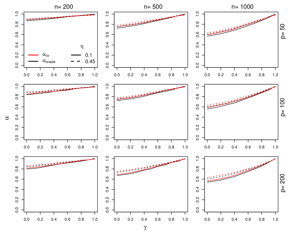
Figure 3: Tuning parameter selection via 10-fold cross-validation. Average oracle tuning parameter $\alpha_{\rm oracle}$ (black) and average optimal cross-validation tuning parameter $\alpha_{\rm CV}$ (red) plotted against the weight parameter $\gamma$ in Equation (4.1), for various scenarios with $K=2$, missingness proportion $\eta=0.1,0.45$, number of variables $p=50,100,200$, and total sample size $n=200,500,1000$. The average $\alpha_{\rm CV}$ and $\alpha_{\rm oracle}$ are very close and both increase with $\gamma$ and decrease with $n$.

4.2 Accuracy of tuning parameter selection

In this simulation, we investigate the behavior of the optimal parameter $\alpha_{\rm CV}$ (Equation (3.6)) selected 10-fold via cross-validation (Algorithm 2) under various settings, and compare it with the oracle tuning parameter

$$\alpha_{\rm oracle}~{}:=~{}\underset{0\leq\alpha\leq 1}{\arg\min}~{}\sum_{(i,j)\in O}(\hat{C}_{ij}(\alpha)-C_{ij})^{2},$$ (4.4)

where $C_{ij}$ is ground truth correlation between variables $(i,j)$. Observing $\alpha_{\rm CV}$ close to $\alpha_{\rm oracle}$ would suggest that our cross-validation procedure is likely to yield a covariance matrix estimate $\hat{\Sigma}(\alpha_{\rm CV})$ that is close to the oracle optimal $\hat{\Sigma}(\alpha_{\rm oracle})$.

We generate ground truth covariance matrix and data as described in Section 4.1 with various settings, $\gamma\in[0,1]$, $p=50,100,200$, $n=200,500,1000$, $K=2$, $\eta=0.1,0.45$, and compute the average $\alpha_{\rm CV}$ and $\alpha_{\rm oracle}$ across $B=50$ simulation repeats. We summarize the results in Figure 3. First, we can see that $\alpha_{\rm CV}$ adequately recovers $\alpha_{\rm oracle}$, although it slightly overestimates it. Moreover, $\alpha_{\rm cv}$ and $\alpha_{\rm oracle}$ both increase with $\gamma$, likely because a larger value of this parameter strengthens the relationship between correlation and auxiliary variable, and so an $\alpha$ closer to 1 gives more weight to the auxiliary baseline covariances rather than to the empirical covariances. Finally, $\alpha_{\rm cv}$ and $\alpha_{\rm oracle}$ increase with $\eta$ and decrease with $n$, presumably because a larger $n$ makes the empirical covariances more reliable over the observed set $O$.

4.3 Accuracy of uncertainty quantification

In this simulation we assess the accuracy of the nonparametric bootstrap (Algorithm 3) and the parametric bootstrap (Algorithm 4) at approximating the standard errors of the AuxCov correlation estimates computed from $\hat{\Sigma}(\alpha_{\rm CV})$ (Algorithms 1–2). In Figure 4, we summarize the results of a simulation with $p=50$, $n=10000$, $K=2$, $\eta=0.1$, and $\gamma=0.5$. We can see that both the nonparametric and the parametric bootstrap methods let us adequately approximate the true standard errors which we approximated via Monte Carlo integration.

Figure 4: Bootstrap. Nonparametric (left) and parametric (right) bootstrap standard errors of AuxCov correlation estimates plotted against the true standard errors approximated via Monte Carlo integration, using $p=50$, $n=10000$, $K=2$, $\eta=0.1$, and $\gamma=0.5$.

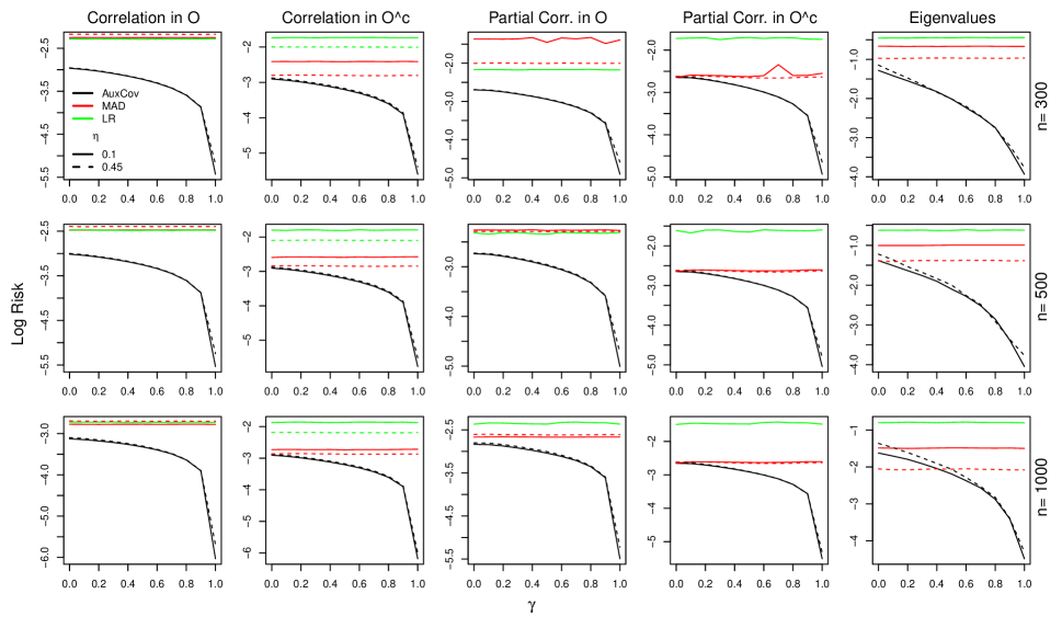
Figure 5: Methods comparison. Performance of AuxCov, MaxDet, and LR at recovering correlations, partial correlations, and eigenvalues for $\gamma\in[0,1]$, $p=50,100,200$, $n=300,500,1000$, $K=2$, $\eta=0.1,0.45$. AuxCov outperforms MaxDet and LR in almost all conditions, especially for larger values of $\gamma$.

4.4 Methods comparison

In this simulation we compare AuxCov with MaxDet (Equation (4.2)) and LR (Equation (4.3)). We generate ground truth covariance matrix and data as described in Section 4.1 with various settings, $\gamma\in[0,1]$, $p=100$, $n=300,500,1000$, $K=2$, $\eta=0.1,0.45$, and evaluate performance using risk metrics based on the following loss functions:

1. Correlation recovery:

   $${\rm loss}(\hat{C}_{O},C_{O}) = (|O|-p)^{-1}\sum_{i\neq j,(i,j)\in O}(\hat{C}_{ij}-C_{ij})^{2},$$ (4.5)

   $${\rm loss}(\hat{C}_{O^{c}},C_{O^{c}}) = |O^{c}|^{-1}\sum_{(i,j)\in O^{c}}(\hat{C}_{ij}-C_{ij})^{2},$$ (4.6)

   where $\hat{C}_{ij}=\hat{\Sigma}_{ij}(\hat{\Sigma}_{ii}\hat{\Sigma}_{jj})^{-1/2}$ and $C_{ij}=\Sigma_{ij}(\Sigma_{ii}\Sigma_{jj})^{-1/2}$ are estimated and ground truth correlations, respectively.

2. Partial correlation recovery:

   $${\rm loss}(\hat{\rho}_{O},\rho_{O}) = (|O|-p)^{-1}\sum_{i\neq j,(i,j)\in O}(\hat{\rho}_{ij}-\rho_{ij})^{2},$$ (4.7)

   $${\rm loss}(\hat{\rho}_{O^{c}},\rho_{O^{c}}) = |O^{c}|^{-1}\sum_{(i,j)\in O^{c}}(\hat{\rho}_{ij}-\rho_{ij})^{2},$$ (4.8)

   where $\hat{\rho}_{ij}=-\hat{\Theta}_{ij}(\hat{\Theta}_{ii}\hat{\Theta}_{jj})^{-1/2}$ and $\rho_{ij}=-\Theta_{ij}(\Theta_{ii}\Theta_{jj})^{-1/2}$ are estimated and ground truth partial correlations, respectively.

3. Eigenvalues recovery:

   $${\rm loss}(\hat{\lambda},\lambda)=p^{-1}\sum_{i=1}^{p}(\hat{\lambda}_{i}-\lambda_{i})^{2}$$ (4.9)

   where $\hat{\lambda}_{i}$ and $\lambda_{i}$ are the $i$-th eigenvalue of $\hat{\Sigma}$ and $i$-th eigenvalue of $\Sigma$, respectively.

In Figure 5 we show the log₁₀ risks computed for the performance assessment about correlation recovery in $O$ and $O^{c}$, partial correlation recovery in $O$ and $O^{c}$, and eigenvalues recovery. We can see that AuxCov outperforms MaxDet and LR in almost all conditions, especially for larger values of $\gamma$.

5 Data analysis

We apply AuxCov to the analysis of neuronal calcium imaging activity traces data (publicly available, [36]) recorded from about 10,000 neurons in a 1mm $\times$ 1mm $\times$ 0.5mm volume of mouse visual cortex (70–385µm depth). The data were recorded in vivo via 2–photon imaging of GCaMP6s with 2.5Hz scan rate [39]. During the experiment, the animal was free to run on an air-floating ball in complete darkness for 105 minutes.

For our analyses, we focus on one layer of the brain portion containing 725 neurons. A graphical illustration of the neurons’ positions is in Figure 6A, where we further depict an observation scheme with two subsets $V_{1}$ and $V_{2}$ of recorded neurons delimited by blue and red contours. The sizes of the contours specify the size of the observed data sets shown in Figure 6B, which induce a missingess proportions $\eta$ in the observed sample covariance matrix depicted in Figure 6C. We implement AuxCov by taking the inter-neuron distance as an auxiliary variable. The relationship between sample correlations and inter-neuron distance was shown in Figure 1. Finally, in Figure 6D we plot the values of the five loss functions defined in Equations (4.5)–(4.9) versus $\eta$, using the sample covariance matrix computed from the full data set as the ground truth covariance matrix. We can see that the performance of AuxCov is robust to different levels of missingness.

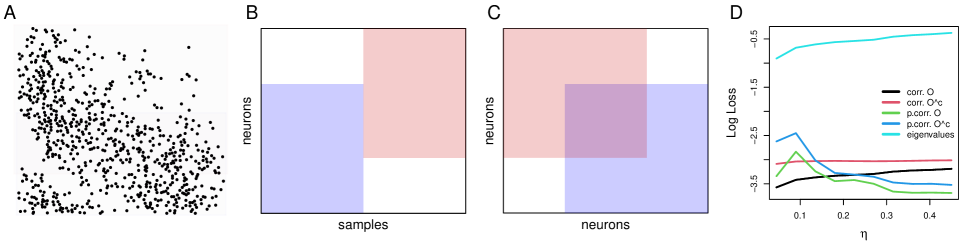
Figure 6: Neuronal data (A): Locations of 725 neurons and two observed subsets $V_{1}$ and $V_{2}$. (B): Incomplete data from observed neurons in (A). (C): Observed sample covariance matrix. (D): Log loss for AuxCov for various amounts of missingness proportion $\eta$.

6 Discussion

In this article we proposed a novel and flexible approach, AuxCov, for the completion of covariance matrix estimates by exploiting auxiliary variables. We illustrated the performance of AuxCov in simulations, where we compared it with other approaches, and in the analysis of neuroscience data, where we used the physical distance between neurons as the auxiliary variable. In simulations, we observed that AuxCov can substantially outperform methods that do not exploit auxiliary information. AuxCov can be applied to the completion of generic incomplete covariance matrix estimators, and the regression method required can be either parametric or nonparametric. We expect AuxCov to be useful in the analysis of large-scale multivariate data from disparate fields of research, as long as auxiliary variables are available.

Appendix

Appendix A Matrix Correction

Let $A$ be a $p\times p$ symmetric matrix with positive diagonals but with negative minimum eigenvalue. A positive definite corrected version of $A$ is given by

$$\tilde{A}={\rm diag}(A)^{1/2}\times\tilde{B}\times{\rm diag}(A)^{1/2},$$ (A.1)

where $\tilde{B}=B+\nu^{*}I_{p}$, $B={\rm diag}(A)^{-1/2}\times A\times{\rm diag}(A)^{-1/2}$, and

$$\nu^{*}=\underset{\nu>0}{\arg\min}~{}\nu$$ (A.2)

$$\text{s.t.}~{}B+\nu I_{p}\succ 0$$ (A.3)

This approach can be implemented efficiently via Algorithm 5:

Input: Symmetric $p\times p$ matrix $A$ with positive diagonals; positive constant $\delta>0$;

1. Compute $B={\rm diag}(A)^{-1/2}\times A\times{\rm diag}(A)^{-1/2}$

2. If $\lambda_{\rm min}(B)\leq 0$, update $B\equiv B+\delta I_{p}$.

3. Repeat step 2 until $\lambda_{\rm min}(B)>0$.

Output: Positive definite matrix

$$\tilde{A}~{}=~{}{\rm diag}(A)^{1/2}\times B\times{\rm diag}(A)^{1/2}$$

Algorithm 5 Positive Definite Matrix Correction

References

- [1] Adam Kohn and Matthew A Smith. Stimulus dependence of neuronal correlation in primary visual cortex of the macaque. Journal of Neuroscience, 25(14):3661–3673, 2005.
- [2] Matthew A Smith and Marc A Sommer. Spatial and temporal scales of neuronal correlation in visual area v4. Journal of Neuroscience, 33(12):5422–5432, 2013.
- [3] Giuseppe Vinci, Valérie Ventura, Matthew A Smith, and Robert E Kass. Separating spike count correlation from firing rate correlation. Neural computation, 28(5):849–881, 2016.
- [4] Giuseppe Vinci, Valérie Ventura, Matthew A Smith, and Robert E Kass. Adjusted regularization in latent graphical models: Application to multiple-neuron spike count data. The annals of applied statistics, 12(2):1068, 2018.
- [5] Giuseppe Vinci, Valérie Ventura, Matthew A Smith, and Robert E Kass. Adjusted regularization of cortical covariance. Journal of computational neuroscience, 45:83–101, 2018.
- [6] Juliane Schäfer and Korbinian Strimmer. A shrinkage approach to large-scale covariance matrix estimation and implications for functional genomics. Statistical applications in genetics and molecular biology, 4(1), 2005.
- [7] Emma Hine and Mark W Blows. Determining the effective dimensionality of the genetic variance–covariance matrix. Genetics, 173(2):1135–1144, 2006.
- [8] T Tony Cai, Hongzhe Li, Weidong Liu, and Jichun Xie. Covariate-adjusted precision matrix estimation with an application in genetical genomics. Biometrika, 100(1):139–156, 2013.
- [9] Luqin Gan, Giuseppe Vinci, and Genevera I Allen. Correlation imputation for single-cell rna-seq. Journal of Computational Biology, 29(5):465–482, 2022.
- [10] Andy Taylor, Benjamin Joachimi, and Thomas Kitching. Putting the precision in precision cosmology: How accurate should your data covariance matrix be? Monthly Notices of the Royal Astronomical Society, 432(3):1928–1946, 2013.
- [11] Jan Niklas Grieb, Ariel G Sánchez, Salvador Salazar-Albornoz, and Claudio Dalla Vecchia. Gaussian covariance matrices for anisotropic galaxy clustering measurements. Monthly Notices of the Royal Astronomical Society, 457(2):1577–1592, 2016.
- [12] Olivier Ledoit and Michael Wolf. Improved estimation of the covariance matrix of stock returns with an application to portfolio selection. Journal of empirical finance, 10(5):603–621, 2003.
- [13] Shaojun Guo, John Leigh Box, and Wenyang Zhang. A dynamic structure for high-dimensional covariance matrices and its application in portfolio allocation. Journal of the American Statistical Association, 112(517):235–253, 2017.
- [14] Samruddhi Deshmukh and Amartansh Dubey. Improved covariance matrix estimation with an application in portfolio optimization. IEEE Signal Processing Letters, 27:985–989, 2020.
- [15] Ming Yuan and Yi Lin. Model selection and estimation in the gaussian graphical model. Biometrika, 94(1):19–35, 2007.
- [16] Jerome Friedman, Trevor Hastie, and Robert Tibshirani. Sparse inverse covariance estimation with the graphical lasso. Biostatistics, 9(3):432–441, 2008.
- [17] Jianqing Fan, Yang Feng, and Yichao Wu. Network exploration via the adaptive lasso and scad penalties. The Annals of Applied Statistics, 3(2):521, 2009.
- [18] Adam J Rothman, Peter J Bickel, Elizaveta Levina, and Ji Zhu. Sparse permutation invariant covariance estimation. Electronic Journal of Statistics, 2:494–515, 2008.
- [19] Peter J Bickel and Elizaveta Levina. Regularized estimation of large covariance matrices. The Annals of Statistics, 36(1):199–227, 2008.
- [20] T Tony Cai, Cun-Hui Zhang, and Harrison H Zhou. Optimal rates of convergence for covariance matrix estimation. The Annals of Statistics, 38(4):2118–2144, 2010.
- [21] Tony Cai and Weidong Liu. Adaptive thresholding for sparse covariance matrix estimation. Journal of the American Statistical Association, pages 672–684, 2011.
- [22] Jacob Bien and Robert J Tibshirani. Sparse estimation of a covariance matrix. Biometrika, 98(4):807–820, 2011.
- [23] Hao Wang. Bayesian graphical lasso models and efficient posterior computation. Bayesian Analysis, 7(4):867–886, 2012.
- [24] Sayantan Banerjee and Subhashis Ghosal. Bayesian structure learning in graphical models. Journal of Multivariate Analysis, 136:147–162, 2015.
- [25] Abdolreza Mohammadi and Ernst C Wit. Bayesian structure learning in sparse gaussian graphical models. Bayesian Analysis, 10(1):109–138, 2015.
- [26] Hao Wang. Scaling it up: Stochastic search structure learning in graphical models. Bayesian Analysis, 10(2):351–377, 2015.
- [27] Wenli Shi, Subhashis Ghosal, and Ryan Martin. Bayesian estimation of sparse precision matrices in the presence of gaussian measurement error. Electronic Journal of Statistics, 15(2):4545–4579, 2021.
- [28] Venkat Chandrasekaran, Pablo A. Parrilo, and Alan S. Willsky. Latent variable graphical model selection via convex optimization. Ann. Statist., 40(4):1935–1967, 08 2012.
- [29] Emmanuel J Candès and Benjamin Recht. Exact matrix completion via convex optimization. Foundations of Computational mathematics, 9(6):717, 2009.
- [30] Emmanuel Candes and Benjamin Recht. Exact matrix completion via convex optimization. Communications of the ACM, 55(6):111–119, 2012.
- [31] Emmanuel J Candès and Yaniv Plan. Matrix completion with noise. Proceedings of the IEEE, 98(6):925–936, 2010.
- [32] Jian-Feng Cai, Emmanuel J Candès, and Zuowei Shen. A singular value thresholding algorithm for matrix completion. SIAM Journal on optimization, 20(4):1956–1982, 2010.
- [33] Arthur P Dempster. Covariance selection. Biometrics, pages 157–175, 1972.
- [34] Robert Grone, Charles R Johnson, Eduardo M Sá, and Henry Wolkowicz. Positive definite completions of partial hermitian matrices. Linear algebra and its applications, 58:109–124, 1984.
- [35] Giuseppe Vinci, Gautam Dasarathy, and Genevera I Allen. Graph quilting: graphical model selection from partially observed covariances. arXiv preprint arXiv:1912.05573, 2019.
- [36] Carsen Stringer, Marius Pachitariu, Nicholas Steinmetz, Charu Bai Reddy, Matteo Carandini, and Kenneth D Harris. Spontaneous behaviors drive multidimensional, brainwide activity. Science, 364(6437):eaav7893, 2019.
- [37] Bradley Efron and Robert J Tibshirani. An introduction to the bootstrap. CRC press, 1994.
- [38] Bradley Efron. Missing data, imputation, and the bootstrap. Journal of the American Statistical Association, 89(426):463–475, 1994.
- [39] Marius Pachitariu, Carsen Stringer, Mario Dipoppa, Sylvia Schröder, L Federico Rossi, Henry Dalgleish, Matteo Carandini, and Kenneth D Harris. Suite2p: beyond 10,000 neurons with standard two-photon microscopy. Biorxiv, page 061507, 2017.