Coded Many-User Multiple Access via
Approximate Message Passing

Abstract

We consider communication over the Gaussian multiple-access channel in the regime where the number of users grows linearly with the codelength. We investigate coded CDMA schemes where each user’s information is encoded via a linear code before being modulated with a signature sequence. We propose an efficient approximate message passing (AMP) decoder that can be tailored to the structure of the linear code, and provide an exact asymptotic characterization of its performance. Based on this result, we consider a decoder that integrates AMP and belief propagation and characterize the tradeoff between spectral efficiency and signal-to-noise ratio, for a given target error rate. Simulation results are provided to demonstrate the benefits of the concatenated scheme at finite lengths.

I Introduction

We consider communication over an $L$-user Gaussian multiple access channel (GMAC), which has output of the form

$$\boldsymbol{y}=\sum_{\ell=1}^{L}\boldsymbol{c}_{\ell}+\boldsymbol{\varepsilon}\,,$$ (1)

over $n$ channel uses. Here $\boldsymbol{c}_{\ell}\in{\mathbb{R}}^{n}$ is the codeword of the $\ell$-th user and $\boldsymbol{\varepsilon}\sim{\mathcal{N}}_{n}(\boldsymbol{0},\sigma^{2}\boldsymbol{I})$ is the channel noise. Motivated by modern applications in machine-type communications, a number of recent works have studied the GMAC in the many-user or many-access setting, where the number of users $L$ grows with the block length $n$ [1, 2, 3, 4].

In this paper, we study the many-user regime where $L,n\to\infty$ with the user density $\mu:=L/n$ converging to a constant. Each user transmits a fixed number of bits $k$ (payload) under a constant energy-per-information-bit constraint $\|\boldsymbol{c}_{\ell}\|^{2}_{2}/k\leq E_{b}$. Moreover, the spectral efficiency is the total user payload per channel use and is denoted by $\mathsf{S}=(Lk)/n=\mu k$. In this regime, a key question is to understand the tradeoff between user density (or spectral efficiency), the signal-to-noise ratio $E_{b}/N_{0}$, and the probability of decoding error. Here $N_{0}=2\sigma^{2}$ is the noise spectral density. A popular measure of decoding performance is the per-user probability of error ($\mathtt{PUPE}$), defined as

$$\mathtt{PUPE}:=\frac{1}{L}\sum_{\ell=1}^{L}\,\mathbb{P}(\boldsymbol{c}_{\ell}\neq\hat{\boldsymbol{c}}_{\ell}),$$ (2)

where $\hat{\boldsymbol{c}}_{\ell}$ is the decoded codeword for user $\ell$.

Polyanskiy [2] and Zadik et al. [3] obtained converse and achievability bounds on the minimum ${E_{b}}/{N_{0}}$ required to achieve $\mathtt{PUPE}\leq\epsilon$ for a given $\epsilon>0$, when the user density $\mu$ and user payload $k$ are fixed. These bounds were extended to the GMAC with Rayleigh fading in [5, 6]. The achievability bounds in these works are obtained using Gaussian random codebooks and joint maximum-likelihood decoding, which is computationally infeasible.

Coding schemes

Efficient coding schemes for the many-user GMAC, based on random linear models and spatial coupling with Approximate Message Passing (AMP) decoding, were proposed in [7]. Using similar ideas, Kowshik obtained improved achievability bounds in [8]. In the schemes proposed in [7], each user’s codeword is produced by directly multiplying a matrix with the user’s information sequence. The simplest such scheme is binary CDMA, where each user $\ell\in[L]$ transmits one bit of information by modulating a signature sequence $\boldsymbol{a}_{\ell}\in{\mathbb{R}}^{n}$, i.e., the codeword $\boldsymbol{c}_{\ell}=\boldsymbol{a}_{\ell}x_{l}$ where $x_{\ell}\in\{\pm\sqrt{E}\}$. Thus the decoding problem is to recover the vector of information symbols $\boldsymbol{x}=[x_{1},\ldots,x_{L}]^{\textsf{T}}$ from the channel output vector

$$\boldsymbol{y}=\sum_{\ell=1}^{L}\boldsymbol{a}_{\ell}x_{\ell}+\boldsymbol{\varepsilon}=\boldsymbol{A}\boldsymbol{x}+\boldsymbol{\varepsilon}\,,$$ (3)

where $\boldsymbol{A}=[\boldsymbol{a}_{1},\ldots,\boldsymbol{a}_{L}]\in{\mathbb{R}}^{n\times L}$ is the matrix of signature sequences. If each user wishes to transmit $k>1$ bits in $n$ channel uses, the binary CDMA scheme requires $k$ blocks of transmission, with each block (and each signature sequence) having length $n/k$.

The optimal spectral efficiency of CDMA in the large system limit (with random signature sequences) has been studied in a number of works, e.g. [9, 10, 11, 12, 13]. Assuming the signature sequences are i.i.d. sub-Gaussian, the best known technique for efficiently decoding $\boldsymbol{x}$ from $\boldsymbol{y}$ in (3) is AMP [14, 15], a family of iterative algorithms that has its origins in relaxations of belief propagation [16, 17]. An attractive feature of AMP decoding is that it allows an exact asymptotic characterization of its error performance through a deterministic recursion called ‘state evolution’.

Main Contributions

The binary CDMA scheme described by (3) transmits uncoded user information. In this paper, we show how the performance can be significantly improved by using a concatenated coding scheme in which each user’s information sequence is first encoded using a linear code before being multiplied with the signature sequence. We propose a flexible AMP decoder that can be tailored to the structure of the linear code, and provide an exact asymptotic characterization of its error performance (Theorem 1). Specifically, we show how a decoder for the underlying code, such as a maximum-likelihood or a belief propagation (BP) decoder, can be incorporated within the AMP algorithm with rigorous asymptotic guarantees (Corollary 1). Simulation results validate the theory and demonstrate the benefits of the concatenated scheme at finite lengths. We focus on binary CDMA to highlight the gains in the simplest setting. The concatenated scheme as well as the AMP decoder and its analysis can be extended to the general random linear model based schemes studied in [7]. These will be described in the extended version of this paper.

We emphasize that our setting is distinct from unsourced random access over the GMAC [2, 18, 19, 20], where all the users share the same codebook and only a subset of them are active. In our case, each user has a distinct signature sequence and all of them are active. While the latter is particularly relevant in designing grant-free communication systems, coding schemes for this setting often rely on dividing a common codebook into sections for different users. Extending the ideas in this paper to unsourced random access is an interesting future direction.

Related Work

AMP algorithms were first proposed for estimation in linear models [14, 15], and have since been applied to a wide range of problems including estimation in generalized linear models and low-rank matrix estimation. We refer the interested reader to[21] for a survey. In the context of communication over AWGN channels, AMP has been used as a decoder for sparse regression codes (SPARCs) [22, 23, 24] and for compressed coding [25]. SPARC-based concatenated schemes with AMP decoding have been proposed for both single-user AWGN channels [26, 27, 28] and unsourced random access[19, 20].

In most of these concatenated schemes [26, 27, 19, 25] the AMP decoder for SPARCs does not explicitly use the structure of the outer code (which is decoded separately). Two key exceptions are the SPARC-LDPC concatenated schemes in [20, 28], which use an AMP decoding algorithm with an integrated BP denoiser. Drawing inspiration from these works, in Section IV-C we propose an AMP decoder with a BP denoiser for our concatenated scheme. Our scheme and its decoder differ from those in [20, 28] in a few important ways: i) we do not use the SPARC message structure, and ii) we treat each user’s codeword as a row of a signal matrix and devise an AMP algorithm with matrix iterates, a notable deviation from prior schemes where AMP operates on vectors.

Notation

We write $[L]$ for the set $\{1,\ldots,L\}$. We use bold uppercase letters for matrices, bold lowercase for vectors, and plain font for scalars. We write $\boldsymbol{a}_{\ell}$ for the $\ell$-th row or column of $\boldsymbol{A}$ depending on the context, and $a_{\ell,i}$ for its $i$th component. A function $f:{\mathbb{R}}^{d}\to{\mathbb{R}}^{d}$ returns a column vector when applied to a column vector, and likewise for row vectors.

II Concatenated coding scheme

The $k$-bit message of user $\ell$, denoted by $\boldsymbol{u}_{\ell}\in\{0,1\}^{k}$, is mapped to a GMAC codeword $\boldsymbol{c}_{\ell}\in{\mathbb{R}}^{n}$ in two steps. First, a rate ${k}/{d}$ linear code with generator matrix $\boldsymbol{G}\in\{0,1\}^{d\times k}$ is used to produce a $d$-bit binary codeword $\boldsymbol{G}\boldsymbol{u}_{\ell}\in\{0,1\}^{d}$. Each $0$ code bit is then mapped to $\sqrt{E}$ and each $1$ bit code bit to $-\sqrt{E}$ to produce $\boldsymbol{x}_{\ell}\in\{\pm\sqrt{E}\}^{d}$. The magnitude $\sqrt{E}$ of each BPSK symbol will be specified later in terms of the energy per bit constraint $E_{b}$. In the second step of encoding, for each user $\ell$, we take the outer-product of $\boldsymbol{x}_{\ell}$ with a signature sequence $\boldsymbol{a}_{\ell}\in{\mathbb{R}}^{\tilde{n}}$, where $\tilde{n}:=n/d.$ This yields a matrix $\boldsymbol{C}_{\ell}=\boldsymbol{a}_{\ell}\boldsymbol{x}_{\ell}^{\top}\in{\mathbb{R}}^{\tilde{n}\times d}$. The final length-$n$ codeword transmitted by user $\ell$ is simply $\boldsymbol{c}_{\ell}=\mathrm{vectorize}(\boldsymbol{C}_{\ell})\in{\mathbb{R}}^{n}$.

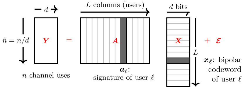
Figure 1: Concatenated coding scheme for GMAC

Let $\boldsymbol{X}=\begin{bmatrix}\boldsymbol{x}_{1},\dots,\boldsymbol{x}_{L}\end{bmatrix}^{\top}\in\{\pm\sqrt{E}\}^{L\times d}$ be the signal matrix whose $\ell$th row $\boldsymbol{x}_{\ell}$ is the bipolar codeword of user $\ell$. Let $\boldsymbol{A}=\begin{bmatrix}\boldsymbol{a}_{1},\dots,\boldsymbol{a}_{L}\end{bmatrix}\in{\mathbb{R}}^{\tilde{n}\times L}$ be the design matrix whose columns are the signature sequences. Then the channel output in (1) can be rewritten into matrix form:

$$\boldsymbol{Y}=\sum_{\ell=1}^{L}\boldsymbol{a}_{\ell}\boldsymbol{x}_{\ell}^{\top}+\boldsymbol{\mathcal{E}}=\boldsymbol{A}\boldsymbol{X}+\boldsymbol{\mathcal{E}}\in{\mathbb{R}}^{\tilde{n}\times d}.$$ (4)

See Fig. 1 for an illustration.

Assumptions

We consider i.i.d. Gaussian signature sequences. Specifically, we choose $A_{i\ell}\stackrel{{\scriptstyle\text{i.i.d.}}}{{\sim}}{\mathcal{N}}(0,1/\tilde{n})$, for $i\in[\tilde{n}],\,\ell\in[L]$. We make the natural assumption that the information bits $\boldsymbol{u}_{\ell}\in\{0,1\}^{k}$ are uniformly random, for each user $\ell\in[L]$. We also assume that the noise variance $\sigma^{2}$ in (1) is known, a mild assumption since the i.i.d. Gaussian signature sequences allow $\sigma^{2}$ to be consistently estimated as $\hat{\sigma}^{2}=\frac{\|\boldsymbol{Y}\|^{2}_{\text{F}}}{n}-Ed\mu$.

We consider the asymptotic limit where $L/n\to\mu$ as $n,L\to\infty$, for a user density $\mu>0$ of constant order. We emphasize that $d$ is fixed and does not scale as $n,L\to\infty$. Therefore $\tilde{n}/L=({n}/{d})/L\to{1}/{(d\mu)}$ is also of constant order.

III AMP decoder

The decoding task is to recover the signal matrix $\boldsymbol{X}$ from the channel observation $\boldsymbol{Y}$ in (4), given the design matrix $\boldsymbol{A}$ and the channel noise variance $\sigma^{2}$. A good decoder must take advantage of the prior distribution on $\boldsymbol{X}$: recall that each row of $\boldsymbol{X}$ is an independent codeword taking values in $\{\pm\sqrt{E}\}^{d}$, defined via the underlying rate $k/d$ linear code. The prior distribution of each row of $\boldsymbol{X}$ induced by the linear code is denoted by $P_{\bar{\boldsymbol{x}}}$. Note that $P_{\bar{\boldsymbol{x}}}$ assigns equal probability to $2^{k}$ vectors in $\{\pm\sqrt{E}\}^{d}$.

The AMP decoder recursively produces estimates $\boldsymbol{X}^{t}\in{\mathbb{R}}^{L\times d}$ of $\boldsymbol{X}$ for iteration $t\geq 0$. This is done via a sequence of denoising functions $\eta_{t}$ that can be tailored to the prior $P_{\bar{\boldsymbol{x}}}$. Starting from an initializer $\boldsymbol{X}^{0}=\boldsymbol{0}_{L\times d}$, for $t\geq 0$ the AMP decoder computes:

$$\boldsymbol{Z}^{t}=\boldsymbol{Y}-\boldsymbol{A}\boldsymbol{X}^{t}+\frac{1}{n}\boldsymbol{Z}^{t-1}\left[\sum_{\ell=1}^{L}\eta_{t-1}^{\prime}\left(\boldsymbol{s}^{t-1}_{\ell}\right)\right]^{\top},$$ (5)

$$\boldsymbol{S}^{t}=\boldsymbol{A}^{\top}\boldsymbol{Z}^{t}+\boldsymbol{X}^{t},$$ (6)

$$\boldsymbol{X}^{t+1}=\eta_{t}\left(\boldsymbol{S}^{t}\right),$$ (7)

where $\eta_{t}:{\mathbb{R}}^{d}\to{\mathbb{R}}^{d}$ applies row-wise to matrix inputs, and $\eta_{t}^{\prime}(\boldsymbol{s})=\frac{\textrm{d}\eta_{t}(\boldsymbol{s})}{\textrm{d}\boldsymbol{s}}\in{\mathbb{R}}^{d\times d}$ is the derivative (Jacobian) of $\eta_{t}$. Quantities with negative indices are set to all-zero matrices. When $d=1$, (5)–(7) reduces to the classical AMP algorithm [15] for estimating a vector signal in a linear model.

State Evolution: In limit as $n,L\to\infty$ (with $L/n\to\mu$), the memory term $\frac{1}{n}\boldsymbol{Z}^{t-1}\left[\sum_{\ell=1}^{L}\eta_{t-1}^{\prime}\left(\boldsymbol{s}^{t-1}_{\ell}\right)\right]^{\top}$ in (5) ensures that the row-wise empirical distribution of $\boldsymbol{Z}^{t}\in{\mathbb{R}}^{\tilde{n}\times d}$ converges to a Gaussian ${\mathcal{N}}_{d}(\boldsymbol{0},\boldsymbol{\Sigma}^{t})$ for $t\geq 1$. Furthermore, the row-wise empirical distribution of $(\boldsymbol{S}^{t}-\boldsymbol{X})\in{\mathbb{R}}^{L\times d}$ also converges to the same Gaussian ${\mathcal{N}}_{d}(\boldsymbol{0},\boldsymbol{\Sigma}^{t})$. The covariance matrix $\boldsymbol{\Sigma}^{t}\in{\mathbb{R}}^{d\times d}$ is iteratively defined via the following state evolution recursion, for $t\geq 0$:

$$\boldsymbol{\Sigma}^{t+1}=\sigma^{2}\boldsymbol{I}+\frac{1}{\delta}\mathbb{E}\left\{[\eta_{t}(\bar{\boldsymbol{x}}+\boldsymbol{g}^{t})-\bar{\boldsymbol{x}}][\eta_{t}(\bar{\boldsymbol{x}}+\boldsymbol{g}^{t})-\bar{\boldsymbol{x}}]^{\top}\right\}.$$ (8)

Here $\boldsymbol{I}$ is the $d\times d$ identity matrix, and $\boldsymbol{g}^{t}\sim{\mathcal{N}}_{d}(\boldsymbol{0},\boldsymbol{\Sigma}^{t})$ is independent from $\bar{\boldsymbol{x}}\sim P_{\bar{\boldsymbol{x}}}$. The expectation in (8) is with respect to $\bar{\boldsymbol{x}}$ and $\boldsymbol{g}^{t}$, and the iteration is initialized with $\boldsymbol{\Sigma}^{0}=(\sigma^{2}+E/\delta)\boldsymbol{I}$.

The convergence of the row-wise empirical distribution of $\boldsymbol{S}^{t}$ to the law of $\bar{\boldsymbol{x}}+\boldsymbol{g}^{t}$ follows by applying standard results in AMP theory [29, 21]. This distributional characterization of $\boldsymbol{S}^{t}$ crucially informs the choice of the denoiser $\eta_{t}$. Specifically, for each row $\ell\in[L]$, the role of the denoiser $\eta_{t}$ is to estimate the codeword $\boldsymbol{x}_{\ell}$ from an observation in zero-mean Gaussian noise with covariance matrix $\boldsymbol{\Sigma}^{t}$. In the next section, we discuss the Bayes-optimal denoiser and two other sub-optimal but computationally efficient denoisers. First, we provide a performance characterization of the AMP decoder with a generic Lipschitz-continuous denoiser in Theorem 1.

Decoding performance after $t$ iterations of AMP decoding can be measured via either the user-error rate $\mathtt{UER}=\frac{1}{L}\sum_{\ell=1}^{L}\mathbbm{1}\{\hat{\boldsymbol{x}}^{t+1}_{\ell}\neq\boldsymbol{x}_{\ell}\}$, or the bit-error rate $\mathtt{BER}=\frac{1}{Ld}\sum_{\ell=1}^{L}\sum_{i=1}^{d}\mathbbm{1}\left\{\hat{x}^{t+1}_{\ell,i}\neq x_{\ell,i}\right\}$. Here $\hat{\boldsymbol{x}}^{t+1}_{\ell}=h_{t}(\boldsymbol{s}^{t}_{\ell})$ is a hard-decision estimate of the codeword $\boldsymbol{x}_{\ell}$, produced using a suitable function $h_{t}$, and $\hat{x}^{t+1}_{\ell,i}$ is the $i$th entry of $\hat{\boldsymbol{x}}^{t+1}_{\ell}$. For example, $h_{t}$ may quantize each entry of $\boldsymbol{x}^{t+1}_{\ell}=\eta_{t}(\boldsymbol{s}^{t}_{\ell})$ to a value in $\pm\sqrt{E}$. We note that the $\mathtt{PUPE}$ defined in (2) is the expected value of the $\mathtt{UER}$.

Theorem 1.

Consider the AMP decoding algorithm in (5)–(7) with Lipschitz continuous denoisers $\eta_{t}:{\mathbb{R}}^{d}\to{\mathbb{R}}^{d}$, for $t\geq 1$. Let $\hat{\boldsymbol{x}}^{t+1}_{\ell}=h_{t}(\boldsymbol{s}^{t}_{\ell})$ be the hard-decision estimate in iteration $t$. The asymptotic $\mathtt{UER}$ and $\mathtt{BER}$ in iteration $t$ satisfy the following almost surely, for $t\geq 1$:

$$\lim_{L\to\infty}\frac{1}{L}\sum_{\ell=1}^{L}\mathbbm{1}\{\hat{\boldsymbol{x}}^{t+1}_{\ell}\neq\boldsymbol{x}_{\ell}\}=\mathbb{P}\left(h_{t}\left(\bar{\boldsymbol{x}}+\boldsymbol{g}^{t}\right)\neq\bar{\boldsymbol{x}}\right),$$ (9)

$$\lim_{L\to\infty}\frac{1}{Ld}\sum_{\ell=1}^{L}\sum_{i=1}^{d}\mathbbm{1}\left\{\hat{x}^{t+1}_{\ell,i}\neq x_{\ell,i}\right\}$$ (10)

$$\quad=\frac{1}{d}\sum_{i=1}^{d}\mathbb{P}\left(\left[h_{t}\left(\bar{x}+g^{t}\right)\right]_{i}\neq\bar{x}_{i}\right).$$

Here $\bar{\boldsymbol{x}}\sim P_{\bar{\boldsymbol{x}}}$ and $\boldsymbol{g}^{t}\sim{\mathcal{N}}_{d}(\boldsymbol{0},\boldsymbol{\Sigma}^{t})$ are independent, with $\boldsymbol{\Sigma}_{t}$ defined by the state evolution recursion in (8).

The proof of the theorem is given in Appendix A.

IV Choice of AMP denoiser $\eta_{t}$

IV-A Bayes-optimal denoiser

Since the row-wise distribution of $\boldsymbol{S}^{t}$ converges to the law of $\bar{\boldsymbol{x}}+\boldsymbol{g}^{t}$, the Bayes-optimal or minimum mean squared error (MMSE) denoiser $\eta_{t}^{\textrm{Bayes}}$ estimates each row $\boldsymbol{X}$ as the following conditional expectation. For $\ell\in[L]$,

$$\boldsymbol{x}^{t+1}_{\ell}=\eta_{t}^{\textrm{Bayes}}(\boldsymbol{s}^{t}_{\ell})=\mathbb{E}\left[\bar{\boldsymbol{x}}\mid\bar{\boldsymbol{x}}+\boldsymbol{g}^{t}=\boldsymbol{s}^{t}_{\ell}\right]$$

$$=\sum_{\boldsymbol{x}^{\prime}\in\mathcal{X}}\boldsymbol{x}^{\prime}\cdot\frac{\exp\left(-\frac{1}{2}(\boldsymbol{x}^{\prime}-2\boldsymbol{s}_{\ell}^{t})^{\top}(\boldsymbol{\Sigma}^{t})^{-1}\boldsymbol{x}^{\prime}\right)}{\sum_{\tilde{\boldsymbol{x}}^{\prime}\in\mathcal{X}}\exp\left(-\frac{1}{2}(\tilde{\boldsymbol{x}}^{\prime}-2\boldsymbol{s}_{\ell}^{t})^{\top}(\boldsymbol{\Sigma}^{t})^{-1}\tilde{\boldsymbol{x}}^{\prime}\right)}$$ (11)

where $\mathcal{X}\subset\{\pm\sqrt{E}\}^{d}$ is the set of $2^{k}$ codewords. Since $\left\lvert\mathcal{X}\right\rvert=2^{k}$, the cost of computing $\eta_{t}^{\textrm{Bayes}}$ grows exponentially in $k$. In each iteration $t$, the decoder can produce a hard-decision maximum a posteriori (MAP) estimate $\hat{\boldsymbol{x}}_{\ell}^{t}$ from $\boldsymbol{s}_{\ell}^{t}$ via:

$$\hat{\boldsymbol{x}}_{\ell}^{t+1}=h_{t}(\boldsymbol{s}_{\ell}^{t})=\operatorname*{arg\,max}_{\boldsymbol{x}^{\prime}\in\mathcal{X}}\mathbb{P}\left(\bar{\boldsymbol{x}}=\boldsymbol{x}^{\prime}\mid\bar{\boldsymbol{x}}+\boldsymbol{g}^{t}=\boldsymbol{s}_{\ell}^{t}\right).$$ (12)

In Section V (Fig. 2) we present numerical results illustrating the performance of AMP with denoiser $\eta_{t}^{\textrm{Bayes}}$ for a Hamming code with $d=7$ and $k=4$. In practical scenarios where $d$ is of the order of several hundreds or thousands, applying $\eta_{t}^{\textrm{Bayes}}$ is not feasible, motivating the use of sub-optimal denoisers with lower computational cost.

IV-B Marginal-MMSE denoiser

A computationally efficient alternative to the Bayes-optimal denoiser is the marginal-MMSE denoiser [26, 19] which acts entry-wise on $\boldsymbol{s}_{\ell}^{t}$ and returns the entry-wise conditional expectation:

$$\boldsymbol{x}_{\ell}^{t+1}=\eta_{t}^{\textrm{marginal}}(\boldsymbol{s}_{\ell}^{t}) =\begin{bmatrix}\mathbb{E}[\bar{x}_{1}|\bar{x}_{1}+g^{t}_{1}=s_{\ell,1}^{t}]\\ \vdots\\ \mathbb{E}[\bar{x}_{d}|\bar{x}_{d}+g^{t}_{d}=s_{\ell,d}^{t}]\end{bmatrix},\text{ where}$$

$$\mathbb{E}[\bar{x}_{i}|\bar{x}_{i}+g^{t}_{i}=s_{\ell,i}^{t}] \stackrel{{\scriptstyle\text{(i)}}}{{=}}\sqrt{E}\tanh\left(\sqrt{E}s_{\ell,i}^{t}/\Sigma_{i,i}^{t}\right).$$ (13)

The equality (i) follows from $g^{t}_{i}\sim{\mathcal{N}}(0,\Sigma^{t}_{i,i})$ and $p(\bar{x}_{i}=\sqrt{E})=p(\bar{x}_{i}=-\sqrt{E})=\frac{1}{2}$ due to the linearity of the outer code. A hard decision estimate $\hat{\boldsymbol{x}}_{\ell}^{t+1}$ can be obtained by quantizing each entry of $\boldsymbol{x}_{\ell}^{t+1}$ to $\{\pm\sqrt{E}\}$.

This marginal denoiser has a computational cost that grows linearly in $d$, but it ignores the parity structure of $\bar{\boldsymbol{x}}$, which is useful prior knowledge that can help reconstruction. One way to address this is by using the output of the AMP decoder as input to a channel decoder for the outer code, as in [19, 27]. In the next subsection, we show how to improve on this approach. Considering an outer LDPC code, we use an AMP denoiser that fully integrates BP decoding.

IV-C Belief Propagation (BP) denoiser

Assume that the binary linear code used to define the concatenated scheme is an LDPC code. We propose a BP denoiser $\eta_{t}^{\textrm{BP}}$ which exploits the parity structure of the LDPC code in each AMP iteration by performing a few rounds of BP on the associated factor graph. Like the other denoisers above, $\eta_{t}^{\textrm{BP}}$ acts row-wise on the effective observation $\boldsymbol{S}^{t}\in{\mathbb{R}}^{L\times d}$. For $\ell\in[L]$, it produces the updated AMP estimate $\boldsymbol{x}_{\ell}^{t+1}$ from $\boldsymbol{s}_{\ell}^{t}$ as follows, using R rounds of BP.

1) For each variable node $i\in[d]$ and check node $j\in[d-k]$, initialise variable-to-check messages (in log-likelihood ratio format) as:

$$L_{i\to j}^{(0)}=\ln\left[\frac{p(s_{\ell,i}^{t}\ |x_{\ell,i}=+\sqrt{E})}{p(s_{\ell,i}^{t}\ |x_{\ell,i}=-\sqrt{E})}\right]=\frac{2\sqrt{E}s_{\ell,i}^{t}}{\Sigma^{t}_{i,i}}=:L(s_{\ell,i}^{t}).$$ (14)

This initialization follows the distributional assumption $s_{\ell,i}^{t}\stackrel{{\scriptstyle\text{d}}}{{=}}\bar{x}_{i}+g^{t}_{i}$, where $g^{t}_{i}\sim{\mathcal{N}}(0,\Sigma^{t}_{i,i})$ and $p(\bar{x}_{i}=\sqrt{E})=p(\bar{x}_{i}=-\sqrt{E})=\frac{1}{2}$.

2) Let $N(i)$ denote the set of neighbouring nodes of node $i.$ For rounds $1\leq\textsf{r}\leq\textsf{R}$, compute the check-to-variable and variable-to-check messages, denoted by $L_{j\to i}^{(\textsf{r})}$ and $L_{i\to j}^{(\textsf{r})}$, as:

$$L_{j\to i}^{(\textsf{r})} =2\tanh^{-1}\left[\prod_{i^{\prime}\in N(j)\setminus i}\tanh\left(\frac{1}{2}L_{i^{\prime}\to j}^{(\textsf{r}-1)}\right)\right],$$ (15)

$$L_{i\to j}^{(\textsf{r})} =L(s_{\ell,i}^{t})+\sum_{j^{\prime}\in N(i)\setminus j}L_{j^{\prime}\to i}^{(\textsf{r})}.$$ (16)

3) Terminate BP after R rounds by computing the final log-likelihood ratio for each variable node $i\in[d]$:

$$L_{i}^{(\textsf{R})}=L(s_{\ell,i}^{t})+\sum_{j^{\prime}\in N(i)}L_{j^{\prime}\to i}^{(\textsf{R})}.$$ (17)

Equations (15)-(17) are the standard BP updates for an LDPC code [30].

4) Compute the updated AMP estimate $\boldsymbol{x}_{\ell}^{t+1}=\eta_{t}^{\textrm{BP}}(\boldsymbol{s}_{\ell}^{t})$, where

$$\left[\eta_{t}^{\textrm{BP}}(\boldsymbol{s}_{\ell}^{t})\right]_{i}=\sqrt{E}\,\tanh\big{(}L_{i}^{(\textsf{R})}/2\big{)},\quad i\in[d].$$ (18)

The RHS above is obtained by converting the final log-likelihood ratio (17) to a conditional expectation, recalling that $x_{\ell,i}$ takes values in $\{\pm\sqrt{E}\}$. Following the standard interpretation of BP as approximating the bit-wise marginal posterior probabilities [30], the expression in (18) can be viewed as an approximation to

$$\mathbb{E}[\bar{x}_{i}\mid\bar{x}_{i}+g_{i}^{t}=s_{\ell,i}^{t}\,,\,\text{parities specified by $N(i)$ satisfied}].$$

We highlight the contrast between the conditional expectation above and the one in (13), which does not use the parity check constraints. As with the marginal-MMSE denoiser, a hard-decision estimate $\hat{\boldsymbol{x}}_{\ell}^{t+1}$ can be obtained by quantizing each entry of $\boldsymbol{x}_{\ell}^{t+1}$ to $\{\pm\sqrt{E}\}$.

While the derivative $\eta_{t}^{\prime}$ for the memory term can be easily calculated for $\eta_{t}^{\textrm{Bayes}}$ and $\eta_{t}^{\textrm{marginal}}$ via direct differentiation, the derivative for $\eta_{t}^{\textrm{BP}}$ is less obvious because it involves R rounds of BP updates (15)-(17). Nevertheless, using the approach in [20, 28], the derivative can be derived in closed form provided the number of BP rounds R is less than the girth of the LDPC factor graph.

Lemma 1.

For $t\geq 1$, consider the AMP decoder with denoiser $\eta_{t}^{\textrm{BP}}:{\mathbb{R}}^{d}\to{\mathbb{R}}^{d}$, where BP is performed for fewer rounds than the girth of the LDPC factor graph. Let

$$\boldsymbol{J}:=\frac{\textrm{d}\eta_{t}^{\textrm{BP}}(\boldsymbol{s}_{\ell}^{t})}{\textrm{d}\boldsymbol{s}_{\ell}^{t}}\in{\mathbb{R}}^{d\times d},\ \ \text{ for }\boldsymbol{s}_{\ell}^{t}\in{\mathbb{R}}^{d}.$$ (19)

Then for $i,h\in[d]$ and $i\neq h,$

$$J_{i,i}=\frac{1}{\Sigma^{t}_{i,i}}\left(E-\left[\eta_{t}^{\textrm{BP}}(\boldsymbol{s}_{\ell}^{t})\right]_{i}^{2}\right),\quad J_{i,h}=0.$$ (20)

The proof is given in Appendix B. Lemma 1 implies that the characterization of the limiting $\mathtt{UER}$ and $\mathtt{BER}$ in Theorem 1 holds for AMP decoding with $\eta^{\textrm{BP}}$.

Corollary 1.

The asymptotic guarantees in Theorem 1 hold for the AMP decoder with any of the three denoisers: $\eta^{\textrm{Bayes}}_{t},\eta^{\textrm{marginal}}_{t}$, and for $\eta^{\textrm{BP}}_{t}$ assuming that the number of BP rounds is less than the girth of the LDPC factor graph.

Proof.

It can be verified by direct differentiation that the $\eta^{\textrm{Bayes}}_{t}$ and $\eta^{\textrm{marginal}}_{t}$ are bounded. For $\eta^{\textrm{BP}}$, we only need to show that $J_{i,i}$ in (20) is bounded for $i\in[d]$. This follows by observing that $\Sigma^{t}_{i,i}>\sigma^{2}$ (from (8)) and $[\eta^{\textrm{BP}}(\boldsymbol{s}_{\ell}^{t})]_{i}^{2}<E$ (from (18)). ∎

V Numerical results

We numerically evaluate the tradeoffs achieved by concatenated coding scheme with different denoisers. For a target $\mathtt{BER}=10^{-4}$, we plot the maximum spectral efficiency $\mathsf{S}=Lk/n=(L/\tilde{n})(k/d)$ achievable as a function of signal-to-noise ratio $E_{b}/N_{0}=(Ed/k)/(2\sigma^{2})$. We use $\mathtt{BER}$ rather than $\mathtt{UER}$ since the $\mathtt{UER}$ of an uncoded scheme degrades approximately linearly with $d$. For each setting, we also plot the achievability and converse bounds from [3], which can be adapted to obtain lower and upper bounds on the maximum spectral efficiency achievable for given values of $E_{b}/N_{0}$, per-user payload $k$, and $\mathtt{PUPE}$. To adapt these bounds to target $\mathtt{BER}$ (rather than target $\mathtt{PUPE}$), we using the random coding assumption that when a codeword is decoded incorrectly, approximately half of its bits are in error, i.e. $\mathbb{E}[\mathtt{BER}]=\frac{1}{2}\mathtt{PUPE}$.

In all the figures, ‘SE’ refers to curves obtained by using the state evolution result of Theorem 1, and ‘AMP’ (indicated by crosses) refers to points obtained via simulation. Fig. 2 compares the uncoded case (i.e. $d=1$) with the concatenated scheme with a $(7,4)$ Hamming code, decoded using AMP with Bayes-optimal denoiser $\eta_{t}^{\textrm{Bayes}}$. Even this simple code provides a savings of over 1dB in the minimum $E_{b}/N_{0}$ required to achieve positive spectral efficiency, compared to the uncoded scheme as well as the converse bound for $k=1$.

Figs. 3 and 4 employ LDPC codes from the IEEE 802.11n standards as outer codes (with code length $d=720$ bits). Fig. 3 compares the decoding performance of AMP with different denoisers: the marginal-MMSE $\eta_{t}^{\textrm{marginal}}$ or the BP denoiser $\eta_{t}^{\textrm{BP}}$ which executes 5 rounds of BP per AMP denoising step. The latter outperforms the former by around 7.5dB since $\eta_{t}^{\textrm{marginal}}$ does not use the parity constraints of the code. The dotted orange curve in Fig. 3 shows that the performance of AMP with $\eta_{t}^{\textrm{marginal}}$ is substantially improved by running a BP decoder (200 rounds) after AMP has converged. However, this additional BP decoding at the end also improves the performance of $\eta_{t}^{\textrm{BP}}$ (blue dotted curve). We observe that the achievable spectral efficiency with $\eta_{t}^{\textrm{BP}}+$ BP is consistently about $40\%$ higher than with $\eta_{t}^{\textrm{marginal}}+$ BP.

Figure 2: Comparison of the uncoded scheme and the concatenated scheme with $(7,4)$ Hamming outer code and denoiser $\eta_{t}^{\textrm{Bayes}}$. $L=20000.$

Fig. 4 compares the performance of the concatenated scheme with LDPC codes with different rates: 1/2 and 5/6. The AMP denoiser is $\eta_{t}^{\textrm{BP}}$, and the dotted curves show the effect of adding BP decoding (200 rounds) after AMP convergence. The code with the higher rate $5/6$ achieves higher spectral efficiency for large values of $E_{b}/N_{0}$, but the rate $1/2$ code achieves positive spectral efficiency for smaller $E_{b}/N_{0}$ values.

In all the figures, the asymptotic performance of AMP, predicted by state evolution, closely tracks its actual performance at large, finite $L$. Moreover, considering a metropolitan area with $10^{6}$ to $10^{7}$ devices and each device active a few times per hour, the user density $\mu$ is typically $10^{-4}$ to $10^{-3}$ [3, Remark 3]. For user densities in this range and per-user payload $k$ on the order of $10^{2}$ to $10^{3}$, the spectral efficiency $\mathsf{S}=\mu k$ is less than 1. In all figures, the concatenated coding schemes exhibit the most substantial improvements for $\mathsf{S}<1$.

Figure 3: Comparison of marginal-MMSE denoiser $\eta_{t}^{\textrm{marginal}}$ (orange) and BP denoiser $\eta_{t}^{\textrm{BP}}$ (blue) for decoding LDPC outer code (with fixed rate 1/2). The dotted plots correspond to AMP decoding coupled with 200 rounds of BP after AMP has converged. $L=2000,d=720$.

Figure 4: Comparison of LDPC outer code with rate 1/2 (blue) or 5/6 (green) under AMP decoding with BP denoiser $\eta_{t}^{\textrm{BP}}$. Dotted curves correspond to AMP decoding coupled with 200 rounds of BP after AMP has converged. $L=2000,d=720$.

VI Discussion

Though we assumed an i.i.d. Gaussian design matrix $\boldsymbol{A}$, using recent results on AMP universality [31, 32], the decoding algorithm and all the theoretical results remain valid for a much broader class of ‘generalized white noise’ matrices. This class includes i.i.d. sub-Gaussian matrices, so the results apply to the popular setting of random binary-valued signature sequences. Figs. 2–4 show that the gap between the spectral efficiency achieved by the concatenated scheme and the converse bounds grows with $E_{b}/N_{0}$. The spectral efficiency of our scheme can be substantially improved by using a spatially coupled design matrix [7]. This will be investigated in an extended version of this paper.

Acknowledgment

We thank Jossy Sayir for sharing his implementation of the belief propagation LDPC decoder.

Appendix A Proof of Theorem 1

The proof is similar to the proof of Theorem 1 in [7]. We begin with a state evolution characterization of the AMP iterates that follows from standard results in the AMP literature [15], [21, Sec. 6.7]. For any Lispchitz test function $\psi:{\mathbb{R}}^{d}\times{\mathbb{R}}^{d}\to{\mathbb{R}}$, we almost surely have:

$$\lim_{L\to\infty}\frac{1}{L}\sum_{\ell=1}^{L}\psi(\boldsymbol{x}_{\ell},\boldsymbol{s}_{\ell}^{t})=\mathbb{E}\left[\psi(\bar{\boldsymbol{x}},\bar{\boldsymbol{x}}+\boldsymbol{g}^{t})\right].$$ (21)

The claims in (9) and (10) require a test function $\psi$ that is defined via indicator functions, and is not Lipschitz. We handle this by sandwiching it between two Lipschitz functions that both converge to the required function in a suitable limit.

We prove (10), and omit the the proof of (9) as it is along the same lines. For $x_{\ell,i}\in\{\pm\sqrt{E}\}$, partition the space ${\mathbb{R}}^{d}$ into two decision regions:

$$\mathcal{D}(x_{\ell,i}):=\left\{\boldsymbol{s}_{\ell}^{t}:\left[\eta_{t}(\boldsymbol{s}_{\ell}^{t})\right]_{i}=x_{\ell,i}\right\},$$ (22)

and note that $\mathbbm{1}\{x_{\ell,i}^{t}=x_{\ell,i}\}=\mathbbm{1}\{\boldsymbol{s}_{\ell}^{t}\in\mathcal{D}(x_{\ell,i})\}$. Let $d(\boldsymbol{v},\mathcal{D}):=\inf\{\|\boldsymbol{v}-\boldsymbol{u}\|_{2}:\boldsymbol{u}\in\mathcal{D}\}$ denote the distance between a vector $\boldsymbol{v}\in{\mathbb{R}}^{d}$ and a set $\mathcal{D}\subset{\mathbb{R}}^{d}.$ For any $\epsilon>0$, define functions $\xi_{\epsilon,+},\xi_{\epsilon,-}:{\mathbb{R}}\times{\mathbb{R}}^{d}\to{\mathbb{R}}$ as follows:

$$\xi_{\epsilon,+}(x_{\ell,i},\boldsymbol{s}_{\ell}^{t}):=\begin{cases}1,\quad\quad\quad\quad\quad\quad\quad\quad\text{if }\boldsymbol{s}_{\ell}^{t}\in\mathcal{D}(x_{\ell,i})\\ 0,\quad\quad\quad\quad\quad\quad\quad\quad\text{if }d(\boldsymbol{s}_{\ell}^{t},\mathcal{D}(x_{\ell,i}))>\epsilon\\ 1-d(\boldsymbol{s}_{\ell}^{t},\mathcal{D}(x_{\ell,i}))/\epsilon,\;\text{otherwise}\end{cases}$$

$$\xi_{\epsilon,-}(x_{\ell,i},\boldsymbol{s}_{\ell}^{t}):=\begin{cases}1,\quad\quad\quad\quad\quad\quad\;\text{if }d(\boldsymbol{s}_{\ell}^{t},\mathcal{D}(x_{\ell,i})^{c})>\epsilon\\ 0,\quad\quad\quad\quad\quad\quad\;\text{if }\boldsymbol{s}_{\ell}^{t}\in\mathcal{D}(x_{\ell,i})^{c}\\ d(\boldsymbol{s}_{\ell}^{t},\mathcal{D}(x_{\ell,i}^{c}))/\epsilon,\,\text{otherwise}\end{cases}.$$

Note that $\xi_{\epsilon,+},\xi_{\epsilon,-}$ are Lipschitz-continuous with Lipschitz constant $1/\epsilon$. Moreover, define $\psi_{\epsilon,+}:{\mathbb{R}}^{d}\times{\mathbb{R}}^{d}\to{\mathbb{R}}$ as

$$\psi_{\epsilon,+}(\boldsymbol{x}_{\ell},\boldsymbol{s}_{\ell}^{t}):=\frac{1}{d}\sum_{i=1}^{d}\xi_{\epsilon,+}(x_{\ell,i},\boldsymbol{s}_{\ell}^{t}),$$ (23)

and define $\psi_{\epsilon,-}$ analogously. Then $\psi_{\epsilon,+},\psi_{\epsilon,-}$, being sums Lipschitz functions, are also Lipschitz.

For any $\epsilon>0$ and $\ell\in[L]$ we have

$$\psi_{\epsilon,-}(\boldsymbol{x}_{\ell},\boldsymbol{s}_{\ell}^{t})\leq\frac{1}{d}\sum_{i=1}^{d}\mathbbm{1}\left\{\boldsymbol{s}_{\ell}^{t}\in\mathcal{D}(x_{\ell,i})\right\}\leq\psi_{\epsilon,+}(\boldsymbol{x}_{\ell},\boldsymbol{s}_{\ell}^{t}).$$ (24)

Applying (21) to $\psi_{\epsilon,-}$ and $\psi_{\epsilon,-}$, we have

$$\begin{split}&\lim_{L\to\infty}\frac{1}{L}\sum_{\ell=1}^{L}\psi_{\epsilon,-}(\boldsymbol{x}_{\ell},\boldsymbol{s}_{\ell}^{t})=\mathbb{E}\left[\psi_{\epsilon,-}(\bar{\boldsymbol{x}},\bar{\boldsymbol{x}}+\boldsymbol{g}^{t})\right],\\ &\lim_{L\to\infty}\frac{1}{L}\sum_{\ell=1}^{L}\psi_{\epsilon,+}(\boldsymbol{x}_{\ell},\boldsymbol{s}_{\ell}^{t})=\mathbb{E}\left[\psi_{\epsilon,+}(\bar{\boldsymbol{x}},\bar{\boldsymbol{x}}+\boldsymbol{g}^{t})\right].\end{split}$$ (25)

The functions $\psi_{\epsilon,-}(\boldsymbol{x}_{\ell},\boldsymbol{s}_{\ell}^{t})$ and $\psi_{\epsilon,+}(\boldsymbol{x}_{\ell},\boldsymbol{s}_{\ell}^{t})$ both converge pointwise to $\frac{1}{d}\sum_{i=1}^{d}\mathbbm{1}\left\{x^{t}_{\ell,i}=x_{\ell,i}\right\}$ as $\epsilon\to 0.$ Thus by the Dominated Convergence Theorem, we have

$$\lim_{\epsilon\to 0}\mathbb{E}\left[\psi_{\epsilon,-}(\bar{\boldsymbol{x}},\bar{\boldsymbol{x}}+\boldsymbol{g}^{t})\right] =\frac{1}{d}\sum_{i=1}^{d}\mathbb{E}\left[\mathbbm{1}\left\{\bar{\boldsymbol{x}}+\boldsymbol{g}^{t}\in\mathcal{D}(\bar{x}_{i})\right\}\right]$$

$$=\lim_{\epsilon\to 0}\mathbb{E}\left[\psi_{\epsilon,+}(\bar{\boldsymbol{x}},\bar{\boldsymbol{x}}+\boldsymbol{g}^{t})\right].$$ (26)

From (24),(25), and (26), we conclude that almost surely:

$$\lim_{\epsilon\to 0}\lim_{L\to\infty}\frac{1}{L}\sum_{\ell=1}^{L}\psi_{\epsilon,-}(\boldsymbol{x}_{\ell},\boldsymbol{s}_{\ell}^{t})=\lim_{\epsilon\to 0}\lim_{L\to\infty}\frac{1}{L}\sum_{\ell=1}^{L}\psi_{\epsilon,+}(\boldsymbol{x}_{\ell},\boldsymbol{s}_{\ell}^{t})$$

$$=\lim_{L\to\infty}\frac{1}{Ld}\sum_{\ell=1}^{L}\sum_{i=1}^{d}\mathbbm{1}\left\{\boldsymbol{s}_{\ell}^{t}\in\mathcal{D}(x_{\ell,i})\right\}$$

$$=\frac{1}{d}\sum_{i=1}^{d}\mathbb{E}\left[\mathbbm{1}\left\{\bar{\boldsymbol{x}}+\boldsymbol{g}^{t}\in\mathcal{D}(\bar{x}_{i})\right\}\right],$$ (27)

which is equivalent to (10). ∎

Appendix B Proof of Lemma 1

Figure 5: Message $L_{j^{\prime}\to i}$ depends on $\{L_{i^{\prime}\to j^{\prime}}\}$ which in turn depend on $\{s_{\ell,i^{\prime}}^{t}\}$ and other unlabelled messages in blue, excluding $s_{\ell,i}^{t}$. The unlabelled messages in blue are independent from $s_{\ell,i}^{t}$ since BP is performed for fewer rounds than girth of the graph.

With R denoting the number of BP rounds, from (18) we have

$$J_{i,i}=\frac{\textrm{d}\left[\eta_{t}^{\textrm{BP}}(\boldsymbol{s}_{\ell}^{t})\right]_{i}}{\textrm{d}s_{\ell,i}^{t}} =\frac{\textrm{d}}{\textrm{d}L_{i}^{(\textsf{R})}}\left(\sqrt{E}\cdot\frac{\exp(L_{i}^{(\textsf{R})})-1}{1+\exp(L_{i}^{(\textsf{R})})}\right)\cdot\frac{\textrm{d}L_{i}^{(\textsf{R})}}{\textrm{d}s_{\ell,i}^{t}}$$

$$\stackrel{{\scriptstyle\text{(i)}}}{{=}}\frac{2\sqrt{E}\exp(L_{i}^{(\textsf{R})})}{(1+\exp(L_{i}^{(\textsf{R})}))^{2}}\cdot\frac{2\sqrt{E}}{\Sigma^{t}_{i,i}}$$

$$=\left(E-\left[\eta_{t}^{\textrm{BP}}(\boldsymbol{s}_{\ell}^{t})\right]_{i}^{2}\right)\cdot\frac{1}{\Sigma^{t}_{i,i}}$$ (28)

where (i) uses the fact that

$$\frac{\textrm{d}L_{i}^{(\textsf{R})}}{\textrm{d}s_{\ell,i}^{t}}\stackrel{{\scriptstyle\text{(ii)}}}{{=}}\frac{\textrm{d}L(s_{\ell,i}^{t})}{\textrm{d}s_{\ell,i}^{t}}\stackrel{{\scriptstyle\text{(iii)}}}{{=}}\frac{2\sqrt{E}}{\Sigma^{t}_{i,i}}.$$ (29)

The equality (iii) follows from (14), and (ii) uses (17), noting that each summand $L_{j^{\prime}\to i}^{(\textsf{R})}$ is a function of the extrinsic messages $\{L_{i^{\prime}\to j^{\prime}}^{(\textsf{R}-1)}\ \text{for}\ i^{\prime}\in N(j^{\prime})\setminus i\}$. The key observation is that the messages $\{L_{i^{\prime}\to j^{\prime}}^{(\textsf{R}-1)}\ \text{for}\ i^{\prime}\in N(j^{\prime})\setminus i\}$ do not depend on $s_{\ell,i}^{t}$, since R is smaller than the girth of the graph. See Fig. 5 for an illustration. Thus, none of the summands $L_{j^{\prime}\to i}^{(\textsf{R})}$ depends on $s_{\ell,i}^{t}$ resulting in $\frac{\textrm{d}}{\textrm{d}s_{\ell,i}^{t}}\sum_{j^{\prime}\in N(i)}L_{j^{\prime}\to i}^{(\textsf{R})}=0.$ Similarly we can show that $J_{i,h}=0.$ ∎

References

- [1] X. Chen, T.-Y. Chen, and D. Guo, “Capacity of Gaussian many-access channels,” IEEE Trans. Inf. Theory, vol. 63, no. 6, pp. 3516–3539, 2017.
- [2] Y. Polyanskiy, “A perspective on massive random-access,” in Proc. IEEE Int. Symp. Inf. Theory, 2017, pp. 2523–2527.
- [3] I. Zadik, Y. Polyanskiy, and C. Thrampoulidis, “Improved bounds on Gaussian MAC and sparse regression via Gaussian inequalities,” in Proc. IEEE Int. Symp. Inf. Theory, 2019, pp. 430–434.
- [4] J. Ravi and T. Koch, “Scaling laws for Gaussian random many-access channels,” IEEE Trans. Inf. Theory, vol. 68, no. 4, pp. 2429–2459, 2022.
- [5] S. S. Kowshik, K. Andreev, A. Frolov, and Y. Polyanskiy, “Energy efficient random access for the quasi-static fading MAC,” in Proc. IEEE Int. Symp. Inf. Theory, 2019, pp. 2768–2772.
- [6] S. S. Kowshik and Y. Polyanskiy, “Fundamental limits of many-user MAC with finite payloads and fading,” IEEE Trans. Inf. Theory, vol. 67, no. 9, pp. 5853–5884, 2021.
- [7] K. Hsieh, C. Rush, and R. Venkataramanan, “Near-optimal coding for many-user multiple access channels,” IEEE Journal on Selected Areas in Information Theory, vol. 3, no. 1, pp. 21–36, 2022.
- [8] S. S. Kowshik, “Improved bounds for the many-user MAC,” in Proc. IEEE Int. Symp. Inf. Theory, 2022, pp. 2874–2879.
- [9] S. Verdu and S. Shamai, “Spectral efficiency of CDMA with random spreading,” IEEE Trans. Inf. Theory, vol. 45, no. 2, pp. 622–640, 1999.
- [10] S. Shamai and S. Verdu, “The impact of frequency-flat fading on the spectral efficiency of CDMA,” IEEE Trans. Inf. Theory, vol. 47, no. 4, pp. 1302–1327, 2001.
- [11] G. Caire, S. Guemghar, A. Roumy, and S. Verdu, “Maximizing the spectral efficiency of coded CDMA under successive decoding,” IEEE Trans. Inf. Theory, vol. 50, no. 1, pp. 152–164, 2004.
- [12] T. Tanaka, “A statistical-mechanics approach to large-system analysis of CDMA multiuser detectors,” IEEE Trans. Inf. Theory, vol. 48, no. 11, pp. 2888–2910, 2002.
- [13] D. Guo and S. Verdú, “Randomly spread CDMA: asymptotics via statistical physics,” IEEE Trans. Inf. Theory, vol. 51, no. 6, pp. 1983–2010, 2005.
- [14] D. L. Donoho, A. Maleki, and A. Montanari, “Message-passing algorithms for compressed sensing,” Proc. Natl. Acad. Sci. U.S.A., vol. 106, no. 45, pp. 18 914–18 919, 2009.
- [15] M. Bayati and A. Montanari, “The dynamics of message passing on dense graphs, with applications to compressed sensing,” IEEE Trans. Inf. Theory, vol. 57, no. 2, pp. 764–785, 2011.
- [16] Y. Kabashima, “A CDMA multiuser detection algorithm on the basis of belief propagation,” J. Phys. A, vol. 36, pp. 11 111–11 121, 2003.
- [17] J. Boutros and G. Caire, “Iterative multiuser joint decoding: unified framework and asymptotic analysis,” IEEE Trans. Inf. Theory, vol. 48, no. 7, pp. 1772–1793, 2002.
- [18] V. K. Amalladinne, J.-F. Chamberland, and K. R. Narayanan, “A coded compressed sensing scheme for unsourced multiple access,” IEEE Trans. Inf. Theory, vol. 66, no. 10, pp. 6509–6533, 2020.
- [19] A. Fengler, P. Jung, and G. Caire, “SPARCs for unsourced random access,” IEEE Trans. Inf. Theory, vol. 67, no. 10, pp. 6894–6915, 2021.
- [20] V. K. Amalladinne, A. K. Pradhan, C. Rush, J.-F. Chamberland, and K. R. Narayanan, “Unsourced random access with coded compressed sensing: Integrating AMP and belief propagation,” IEEE Trans. Inf. Theory, vol. 68, no. 4, pp. 2384–2409, 2022.
- [21] O. Y. Feng, R. Venkataramanan, C. Rush, and R. J. Samworth, “A unifying tutorial on approximate message passing,” Foundations and Trends in Machine Learning, vol. 15, no. 4, pp. 335–536, 2022.
- [22] J. Barbier and F. Krzakala, “Approximate message-passing decoder and capacity achieving sparse superposition codes,” IEEE Trans. Inf. Theory, vol. 63, no. 8, pp. 4894–4927, Aug. 2017.
- [23] C. Rush, A. Greig, and R. Venkataramanan, “Capacity-achieving sparse superposition codes via approximate message passing decoding,” IEEE Trans. Inf. Theory, vol. 63, no. 3, pp. 1476–1500, Mar. 2017.
- [24] R. Venkataramanan, S. Tatikonda, and A. Barron, “Sparse regression codes,” Foundations and Trends® in Communications and Information Theory, vol. 15, no. 1-2, pp. 1–195, 2019.
- [25] S. Liang, C. Liang, J. Ma, and L. Ping, “Compressed coding, AMP-based decoding, and analog spatial coupling,” IEEE Trans. Commun., vol. 68, no. 12, pp. 7362–7375, 2020.
- [26] A. Greig and R. Venkataramanan, “Techniques for improving the finite length performance of sparse superposition codes,” IEEE Trans. Commun., vol. 66, no. 3, pp. 905–917, 2018.
- [27] H. Cao and P. O. Vontobel, “Using list decoding to improve the finite-length performance of sparse regression codes,” IEEE Trans. Commun., vol. 69, no. 7, pp. 4282–4293, 2021.
- [28] J. R. Ebert, J.-F. Chamberland, and K. R. Narayanan, “On sparse regression LDPC codes,” in Proc. IEEE Int. Symp. Inf. Theory, 2023.
- [29] A. Javanmard and A. Montanari, “State evolution for general approximate message passing algorithms, with applications to spatial coupling,” Information and Inference: A Journal of the IMA, vol. 2, no. 2, pp. 115–144, 2013.
- [30] T. Richardson and R. Urbanke, Modern Coding Theory. Cambridge University Press, 2008.
- [31] T. Wang, X. Zhong, and Z. Fan, “Universality of approximate message passing algorithms and tensor networks,” 2022, arXiv:2206.13037.
- [32] N. Tan, J. Scarlett, and R. Venkataramanan, “Approximate message passing with rigorous guarantees for pooled data and quantitative group testing,” 2023, arXiv:2309.15507.