On diffusion models for amortized inference:
Benchmarking and improving stochastic control and sampling

Abstract

We study the problem of training diffusion models to sample from a distribution with a given unnormalized density or energy function. We benchmark several diffusion-structured inference methods, including simulation-based variational approaches and off-policy methods (continuous generative flow networks). Our results shed light on the relative advantages of existing algorithms while bringing into question some claims from past work. We also propose a novel exploration strategy for off-policy methods, based on local search in the target space with the use of a replay buffer, and show that it improves the quality of samples on a variety of target distributions. Our code for the sampling methods and benchmarks studied is made public at github.com/GFNOrg/gfn-diffusion as a base for future work on diffusion models for amortized inference.

1 Introduction

Approximating and sampling from complex multivariate distributions is a fundamental problem in probabilistic deep learning (e.g., Hernández-Lobato & Adams, 2015; Izmailov et al., 2021; Harrison et al., 2024) and in scientific applications (Albergo et al., 2019; Noé et al., 2019; Jing et al., 2022; Adam et al., 2022; Holdijk et al., 2023). The problem of drawing samples from a distribution given only an unnormalized probability density or energy is particularly challenging in high-dimensional spaces and when the distribution of interest has many separated modes (Bandeira et al., 2022). Sampling methods based on Markov chain Monte Carlo (MCMC) – such as Metropolis-adjusted Langevin (MALA; Grenander & Miller, 1994; Roberts & Tweedie, 1996; Roberts & Rosenthal, 1998) and Hamiltonian MC (HMC; Duane et al., 1987; Hoffman et al., 2014) – may be slow to mix between modes and have a high cost per sample. While variants such as sequential MC (SMC; Halton, 1962; Chopin, 2002; Del Moral et al., 2006) and nested sampling (Skilling, 2006; Buchner, 2021; Lemos et al., 2023) have better mode coverage, their cost may grow prohibitively with the dimensionality of the problem. This motivates the use of amortized variational inference, i.e., fitting parametric models that sample the target distribution.

Diffusion models, continuous-time stochastic processes that gradually evolve a simple distribution to a complex target, are powerful density estimators with proven mode-mixing properties (De Bortoli, 2022); as such, they have been widely used in the setting of generative models learned from data (Sohl-Dickstein et al., 2015; Song et al., 2021b; Ho et al., 2020; Nichol & Dhariwal, 2021; Rombach et al., 2021). However, the problem of training diffusion models to sample from a distribution with a given black-box density or energy function has attracted less attention. Recent work has drawn connections between diffusion (learning the denoising process) and stochastic control (learning the Föllmer drift), leading to approaches such as the path integral sampler (PIS; Zhang & Chen, 2022), denoising diffusion sampler (DDS; Vargas et al., 2023), and time-reversed diffusion sampler (DIS; Berner et al., 2022); such approaches were recently unified by Richter et al. (2023). Another line of work (Lahlou et al., 2023; Zhang et al., 2024) is based on continuous generative flow networks (GFlowNets), which are deep reinforcement learning algorithms adapted to variational inference that offer stable off-policy training and thus flexible exploration (Malkin et al., 2023).

Unfortunately, the advances in sampling methods have not been accompanied by comprehensive benchmarking: the reproducibility of the results is often unclear, with the works differing in the choice of model architectures, using unstated hyperparameters, and even disagreeing in their definitions of the same target densities. The first main contribution of this paper is a unified library for diffusion-structured amortized inference methods. The library has a focus on off-policy methods (continuous GFlowNets) but also includes simulation-based variational objectives such as PIS. Using this codebase, we are able to benchmark methods from past work under comparable conditions and confirm claims about exploration strategies and desirable inductive biases, while calling into question other claims on the robustness and efficiency of credit assignment. Our library also includes several new modeling and training techniques, and we provide preliminary evidence of their utility in possible future work (§5.3).

Our second main contribution is a study of methods for improving credit assignment – the propagation of learning signals from the target density to the parameters of earlier sampling steps – in diffusion-structured samplers (§4). First, our results (§5.2) suggest that the technique of utilizing partial trajectory information (Madan et al., 2022; Pan et al., 2023), as done in the diffusion setting by Zhang et al. (2024), offers little benefit, and a higher training cost, over on-policy (Zhang & Chen, 2022) or off-policy (Lahlou et al., 2023) trajectory-based optimization. Second, we examine the utility of a gradient-based variant which parametrizes the denoising distribution as a correction to a Langevin process (Zhang & Chen, 2022). We show that this inductive bias is also beneficial in the off-policy (GFlowNet) setting despite higher computational cost. Finally, motivated by recent approaches in the discrete state space setting, we propose an efficient exploration technique based on local search in the target space with the use of a replay buffer, which improves sample quality across various target distributions.

2 Prior work

Amortized variational inference (VI) approaches utilize a parametric model $q_{\theta}$ to approximate a given target density $p_{\rm target}$ through stochastic optimization (Hoffman et al., 2013; Ranganath et al., 2014; Agrawal & Domke, 2021). Notably, explicit density models like autoregressive models and normalizing flows have been extensively utilized in density estimation (Rezende & Mohamed, 2015; Dinh et al., 2017; Wu et al., 2020; Gao et al., 2020; Nicoli et al., 2020). However, these models impose structural constraints, thereby limiting their expressive power (Cornish et al., 2020; Grathwohl et al., 2019; Zhang & Chen, 2021).

The adoption of diffusion processes in generative models has stimulated a renewed interest in hierarchical models as density estimators and paved the way for more sophisticated sampling methodologies (Vincent, 2011; Ho et al., 2020; Tzen & Raginsky, 2019b). Approaches like PIS (Zhang & Chen, 2022) leverage stochastic optimal control for sampling from unnormalized densities, albeit still struggling with scalability in high-dimensional spaces.

Finally, GFlowNets, originally defined in the discrete case by Bengio et al. (2021, 2023), view hierarchical sampling (i.e., stepwise generation) as a sequential decision-making process and represent a synthesis of reinforcement learning and variational inference approaches (Malkin et al., 2023; Zimmermann et al., 2023; Tiapkin et al., 2023), expanding from specific scientific domains (e.g., Jain et al., 2022; Atanackovic et al., 2023; Zhu et al., 2023) to amortized inference over a broader array of latent structures (e.g., van Krieken et al., 2023; Hu et al., 2024). Their ability to efficiently navigate trajectory spaces via off-policy exploration has been crucial, yet they encounter challenges in training dynamics, such as credit assignment and exploration efficiency (Malkin et al., 2022; Madan et al., 2022; Pan et al., 2023; Rector-Brooks et al., 2023; Shen et al., 2023; Kim et al., 2023; Jang et al., 2024). These challenges have repercussions in the scalability of these methods in more complex scenarios, a challenge this paper addresses in the continuous case.

3 Setting: Diffusion-structured sampling

Let ${\mathcal{E}}:{\mathbb{R}}^{d}\to{\mathbb{R}}$ be a differentiable energy function and define $R({\mathbf{x}})=\exp(-{\mathcal{E}}({\mathbf{x}}))$, the reward or unnormalized target density. Assuming the integral $Z:=\int_{{\mathbb{R}}^{d}}R({\mathbf{x}})\,d{\mathbf{x}}$ exists, ${\mathcal{E}}$ defines a Boltzmann density $p_{\rm target}({\mathbf{x}})=\frac{R({\mathbf{x}})}{Z}$ on ${\mathbb{R}}^{d}$. We are interested in the problems of sampling from $p_{\rm target}$ and approximating the partition function $Z$ given access only to ${\mathcal{E}}$ and possibly to its gradient $\nabla{\mathcal{E}}$.

We describe two closely related perspectives on this problem: via neural SDEs and stochastic control (§3.1) and via continuous generative flow networks (§3.2).

3.1 Euler-Maruyama hierarchical samplers

Generative modeling with SDEs.

Diffusion models assume a continuous-time generative process given by a neural stochastic differential equation (SDE; Tzen & Raginsky, 2019a; Øksendal, 2003; Särkkä & Solin, 2019):

$$d{\mathbf{x}}_{t}=u({\mathbf{x}}_{t},t;\theta)\,dt+g({\mathbf{x}}_{t},t;\theta)\,d{\mathbf{w}}_{t},$$ (1)

where ${\mathbf{x}}_{0}$ follows a fixed tractable distribution $\mu_{0}$ (such as a Gaussian or a point mass). The initial distribution $\mu_{0}$ and the stochastic dynamics specified by (1) induce marginal densities $p_{t}$ on ${\mathbb{R}}^{d}$ for each $t>0$. The functions $u$ and $g$ have learnable parameters that we wish to optimize, using some objective, so as to make the terminal density $p_{1}$ close to $p_{\rm target}$. Samples can be drawn from $p_{1}$ by sampling ${\mathbf{x}}_{0}\sim\mu_{0}$ and simulating the SDE (1) to time $t=1$.

The SDE driving $\mu_{0}$ to $p_{\rm target}$ is not unique. However, if one fixes a reverse-time SDE, or noising process, that pushes $p_{\rm target}$ at $t=1$ to $\mu_{0}$ at $t=0$, then its reverse, the forward SDE (1), is uniquely determined under mild conditions and is called the denoising process. For usual choices of the noising process, there are stochastic regression objectives for learning the drift $u$ of the denoising process given samples from $p_{\rm target}$, and the diffusion rate $g$ is available in closed form (Ho et al., 2020; Song et al., 2021b).

Time discretization.

In practice, the integration of the SDE (1) is approximated by a discrete-time scheme, the simplest of which is Euler-Maruyama integration. The process (1) is replaced by a discrete-time Markov chain ${\mathbf{x}}_{0}\rightarrow{\mathbf{x}}_{\Delta t}\rightarrow{\mathbf{x}}_{2\Delta t}\rightarrow\dots\rightarrow{\mathbf{x}}_{1}$, where $\Delta t=\frac{1}{T}$ is the time increment and and $T$ is the number of steps:

$${\mathbf{x}}_{0} \sim\mu_{0},$$ (2)

$${\mathbf{x}}_{t+\Delta t} ={\mathbf{x}}_{t}+u({\mathbf{x}}_{t},t;\theta)\Delta t+g({\mathbf{x}}_{t},t;\theta)\sqrt{\Delta t}\,{\mathbf{z}}_{t}\quad{\mathbf{z}}_{t}\sim\mathcal{N}(\bm{0},{\mathbf{I}}_{d}).$$

The density of the transition kernel from ${\mathbf{x}}_{t}$ to ${\mathbf{x}}_{t+\Delta t}$ can explicitly be written as

$$p_{F}({\mathbf{x}}_{t+\Delta t}\mid{\mathbf{x}}_{t})={\mathcal{N}}({\mathbf{x}}_{t+\Delta t};{\mathbf{x}}_{t}+u({\mathbf{x}}_{t},t;\theta)\Delta t,g({\mathbf{x}}_{t},t;\theta)\Delta t{\mathbf{I}}_{d}),$$ (3)

where $p_{F}$ denotes the transition density of the discretized forward SDE. This density defines a joint distribution over trajectories starting at ${\mathbf{x}}_{0}$:

$$p_{F}({\mathbf{x}}_{\Delta t},\dots,{\mathbf{x}}_{1}\mid{\mathbf{x}}_{0})=\prod_{i=0}^{T-1}p_{F}({\mathbf{x}}_{(i+1)\Delta t}\mid{\mathbf{x}}_{i\Delta t}).$$ (4)

Similarly, a discrete-time reverse process ${\mathbf{x}}_{1}\rightarrow{\mathbf{x}}_{1-\Delta t}\rightarrow{\mathbf{x}}_{1-2\Delta t}\rightarrow\dots\rightarrow{\mathbf{x}}_{0}$ with transition densities $p_{B}({\mathbf{x}}_{t-\Delta t}\mid{\mathbf{x}}_{t})$ defines a joint distribution via

$$p_{B}({\mathbf{x}}_{0},\dots,{\mathbf{x}}_{1-\Delta t}\mid{\mathbf{x}}_{1})=\prod_{t=1}^{T}p_{B}({\mathbf{x}}_{(i-1)\Delta t}\mid{\mathbf{x}}_{i\Delta t}).$$ (5)

If the forward and backward processes (starting from $\mu_{0}$ and $p_{\rm target}$, respectively) are reverses of each other, then they define the same distribution over trajectories, i.e., for all ${\mathbf{x}}_{0}\rightarrow{\mathbf{x}}_{\Delta t}\rightarrow\dots\rightarrow{\mathbf{x}}_{1}$,

$$\mu_{0}({\mathbf{x}}_{0})p_{F}({\mathbf{x}}_{\Delta t},\dots,{\mathbf{x}}_{1}|{\mathbf{x}}_{0})=p_{\rm target}({\mathbf{x}}_{1})p_{B}({\mathbf{x}}_{0},\dots,{\mathbf{x}}_{1-\Delta t}|{\mathbf{x}}_{1}).$$ (6)

In particular, the marginal densities of ${\mathbf{x}}_{1}$ under the forward and backward processes are then equal to $p_{\rm target}$, and the forward process can be used to sample the target distribution.

In practice, (6) can be enforced only approximately, since the reverse of a process with Gaussian increments is, in general, not itself Gaussian. However, the discrepancy vanishes as $\Delta t\to 0$ (i.e., increments are infinitesimally Gaussian), an application of the central limit theorem that is key to stochastic calculus (Øksendal, 2003).

SDE learning as hierarchical variational inference.

The problem of learning the parameters $\theta$ of the forward process so as to enforce (6) is one of hierarchical variational inference. The backward process transforms ${\mathbf{x}}_{1}$ into ${\mathbf{x}}_{0}$ via a sequence of latent variables ${\mathbf{x}}_{1-\Delta t},\dots,{\mathbf{x}}_{0}$, and the forward process aims to match the posterior distribution over these variables and thus to approximately enforce (6).

In the setting of diffusion models learned from data, where one has samples from $p_{\rm target}$, one can optimize the forward process by minimizing the KL divergence $D_{\mathrm{KL}}(p_{\rm target}\cdot p_{B}\|\mu_{0}\cdot p_{F})$ between the distribution over trajectories given by the reverse process and that given by the forward process. This is equivalent to the typical training of diffusion models, which optimizes a variational bound on the data log-likelihood (see Song et al., 2021a).

However, in the setting of an intractable density $p_{\rm target}$, unbiased estimators of this divergence are not available. Instead, one can optimize the reverse KL:

$$D_{\mathrm{KL}}(\mu_{0}\cdot p_{F}\|p_{\rm target}\cdot p_{B})=$$ (7)

$$\int\log\frac{\mu_{0}(x_{0})p_{F}({\mathbf{x}}_{\Delta t},\dots,{\mathbf{x}}_{1}\mid{\mathbf{x}}_{0})}{p_{\rm target}(x_{1})p_{B}({\mathbf{x}}_{0},\dots,{\mathbf{x}}_{1-\Delta t}\mid{\mathbf{x}}_{1})}\mu_{0}({\mathbf{x}}_{0})\,d{\mathbf{x}}_{\Delta t}\,\dots\,d{\mathbf{x}}_{1}.$$

Various estimators of this objective are available. For instance, the path integral sampler objective (PIS; Zhang & Chen, 2022) uses the reparametrization trick to express (7) as an expectation over noise variables ${\mathbf{z}}_{t}$ that participate in the hierarchical sampling of ${\mathbf{x}}_{\Delta t},\dots,{\mathbf{x}}_{1}$, yielding an unbiased gradient estimator, but one that requires backpropagation into the simulation of the forward process. The related denoising diffusion sampler (DDS; Vargas et al., 2023) applies the same principle in a different integration scheme.

3.2 Euler-Maruyama samplers as GFlowNets

Continuous generative flow networks (Lahlou et al., 2023) express the problem of enforcing (6) as a reinforcement learning task. In this section, we summarize this interpretation, its connection to neural SDEs, the associated learning objectives, and their relative advantages and disadvantages.

The connection between generative flow networks and diffusion models was first made informally by Malkin et al. (2023) in the distribution-matching setting and by Zhang et al. (2023a) in the maximum-likelihood setting. Continuous GFlowNets, and their connection to sampling via Euler-Maruyama integration, were first set on a solid theoretical foundation by Lahlou et al. (2023).

State and action space.

To formulate sampling as a sequential decision-making problem, one must define the spaces of states and actions. In the case of sampling by $T$-step Euler-Maruyama integration, assuming $\mu_{0}$ is a point mass at $\bm{0}$, the state space is

$${\mathcal{S}}=\{(\bm{0},0)\cup\left\{({\mathbf{x}},t):{\mathbf{x}}\in{\mathbb{R}}^{d},t\in\{\Delta t,2\Delta t,\dots,1\}\right\},$$

with the point $({\mathbf{x}},t)$ representing that the sampling agent is at position ${\mathbf{x}}$ at time $t$.

Sampling begins with the initial state ${\mathbf{x}}_{0}:=(\bm{0},0)$, proceeds through a sequence of states $({\mathbf{x}}_{\Delta t},\Delta t)$, $({\mathbf{x}}_{2\Delta t},2\Delta t)$, $\dots$, and ends at a state $({\mathbf{x}}_{1},1)$; states $({\mathbf{x}},t)$ with $t=1$ are called terminal states and their collection is denoted ${\mathcal{X}}$. From now on, we will often write ${\mathbf{x}}_{t}$ in place of the state $({\mathbf{x}}_{t},t)$ when the time $t$ is clear from context. The sequence of states ${\mathbf{x}}_{0}\rightarrow{\mathbf{x}}_{\Delta t}\rightarrow\dots\rightarrow{\mathbf{x}}_{1}$ is called a complete trajectory.

The actions from a nonterminal state $({\mathbf{x}}_{t},t)$ correspond to the possible next states $({\mathbf{x}}_{t+\Delta t},t+\Delta t)$ that can be reached from $({\mathbf{x}}_{t},t)$ by a single step of the Euler-Maruyama integrator.

Forward policy and learning problem.

A (forward) policy is a collection of continuous distributions over the successor states – states reachable by a single action – of every nonterminal state $({\mathbf{x}},t)$. In our context, this amounts to a collection of conditional probability densities $p_{F}({\mathbf{x}}_{t+\Delta t}\mid{\mathbf{x}}_{t};\theta)$, representing the probability density of transitioning from ${\mathbf{x}}_{t}$ to ${\mathbf{x}}_{t+\Delta t}$. GFlowNet training optimizes the parameters $\theta$, which may be the weights of a neural network specifying a density over ${\mathbf{x}}_{t+\Delta t}$ conditioned on ${\mathbf{x}}_{\Delta t}$.

A policy $p_{F}$ induces a distribution over complete trajectories $\tau=({\mathbf{x}}_{0}\rightarrow{\mathbf{x}}_{\Delta t}\rightarrow\dots\rightarrow{\mathbf{x}}_{1})$ via

$$p_{F}(\tau;\theta)=\prod_{i=0}^{T-1}p_{F}({\mathbf{x}}_{(i+1)\Delta t}\mid{\mathbf{x}}_{i\Delta t};\theta).$$

In particular, we get a marginal density over terminal states:

$$p_{F}^{\top}({\mathbf{x}}_{1};\theta)\!\!=\!\!\int p_{F}({\mathbf{x}}_{0}\rightarrow{\mathbf{x}}_{\Delta t}\rightarrow\dots\rightarrow{\mathbf{x}}_{1};\theta)\,d{\mathbf{x}}_{\Delta t}\dots d{\mathbf{x}}_{1-\Delta t}.$$ (8)

The learning problem solved by GFlowNets is to find the parameters $\theta$ of a policy $p_{F}$ whose terminating density $p_{F}^{\top}$ is equal to $p_{\rm target}$, i.e.,

$$p_{F}^{\top}({\mathbf{x}}_{1};\theta)=\frac{R({\mathbf{x}}_{1})}{Z}\quad\forall{\mathbf{x}}_{1}\in{\mathbb{R}}^{d}.$$ (9)

However, because the integral (8) is intractable and $Z$ is unknown, auxiliary objects must be introduced into optimization objectives to enforce (9), as discussed below.

Notably, if the policy is a Gaussian with mean and variance given by neural networks taking ${\mathbf{x}}_{t}$ and $t$ as input, then learning the policy amounts to learning the drift $u({\mathbf{x}}_{t},t;\theta)$ and diffusion $g({\mathbf{x}}_{t},t;\theta)$ of a SDE (1), i.e., fitting a neural SDE. The learning problem in §3.1 is thus the same as that of fitting a GFlowNet with Gaussian policies.

Backward policy and trajectory balance.

A backward policy is a collection of conditional probability densities $p_{B}({\mathbf{x}}_{t-\Delta t}\mid{\mathbf{x}}_{t};\psi)$, representing a probability density of transitioning from ${\mathbf{x}}_{t}$ to an ancestor state ${\mathbf{x}}_{t-\Delta t}$. The backward policy induces a distribution over complete trajectories $\tau$ conditioned on their terminal state (cf. (5)):

$$p_{B}(\tau\mid{\mathbf{x}}_{1};\psi;\psi)=\prod_{i=1}^{T}p_{B}({\mathbf{x}}_{(i-1)\Delta t}\mid{\mathbf{x}}_{i\Delta t};\psi),$$

where exceptionally $p_{B}({\mathbf{x}}_{0}\mid{\mathbf{x}}_{\Delta t})=1$ as $\mu_{0}$ is a point mass.

Generalizing a result in the discrete-space setting (Malkin et al., 2022), Lahlou et al. (2023) show that $p_{F}$ samples from the target distribution (i.e., satisfies (9)) if and only if there exists a backward policy $p_{B}$ and a scalar $Z_{\theta}$ such that the trajectory balance conditions are fulfilled for every complete trajectory $\tau=({\mathbf{x}}_{0}\rightarrow{\mathbf{x}}_{\Delta t}\rightarrow\dots\rightarrow{\mathbf{x}}_{1})$:

$$Z_{\theta}p_{F}(\tau;\theta)=p_{\rm target}({\mathbf{x}}_{1})p_{B}(\tau\mid{\mathbf{x}}_{1};\psi).$$ (10)

If these conditions hold, then $Z_{\theta}$ equals the true partition function $Z=\int_{\mathbf{x}}R({\mathbf{x}})\,d{\mathbf{x}}$. The trajectory balance objective for a trajectory $\tau$ is the squared log-ratio of the two sides of (10), that is:

$${\mathcal{L}}_{\rm TB}(\tau;\theta,\psi)=\left(\log\frac{Z_{\theta}p_{F}(\tau;\theta)}{p_{\rm target}({\mathbf{x}}_{1})p_{B}(\tau\mid{\mathbf{x}}_{1};\psi)}\right)^{2}.$$ (11)

One can thus achieve (9) by minimizing to zero the loss ${\mathcal{L}}_{\rm TB}(\tau;\theta,\psi)$ with respect to the parameters $\theta$ and $\psi$, where the trajectories $\tau$ used for training are sampled from some training policy $\pi(\tau)$. While it is possible to optimize (11) with respect to the parameters of both the forward and backward policies, in some learning problems, one fixes the backward policy and only optimizes the parameters of $p_{F}$ and the estimate of the partition function $Z_{\theta}$. For example, for most experiments in §5, we fix the backward policy to a discretized Brownian bridge, following past work.

Off-policy optimization.

Unlike the KL objective (7), whose gradient involves an expectation over the distribution of trajectories under the forward process, (11) can be optimized off-policy, i.e., using trajectories sampled from an arbitary distribution $\pi$. Because minimizing ${\mathcal{L}}_{\rm TB}(\tau;\theta,\psi)$ to 0 for all $\tau$ in the support of $\pi$ will achieve (9), $\pi$ can be taken be any distribution with full support, so as to promote discovery of modes of the target distribution. Various choices motivated by reinforcement learning techniques have been proposed, including noisy exploration or tempering (Bengio et al., 2021), replay buffers (Deleu et al., 2022), Thompson sampling (Rector-Brooks et al., 2023), and backward traces from terminal states obtained by MCMC (Lemos et al., 2023). In the continuous case, Malkin et al. (2023); Lahlou et al. (2023) proposed to simply add a small constant to the policy variance when sampling trajectories for training. Off-policy optimization is a key advantage of GFlowNets over variational methods such as PIS, which require on-policy optimization (Malkin et al., 2023).

However, when ${\mathcal{L}}_{\rm TB}$ happens to be optimized on policy, i.e., using trajectories sampled from the policy $p_{F}$ itself, we get an unbiased estimator of the gradient of the KL divergence with respect to $p_{F}$’s parameters up to a constant (Malkin et al., 2023; Zimmermann et al., 2023), that is:

$${\mathbb{E}}_{\tau\sim p_{F}(\tau)}\left[\nabla_{\theta}{\mathcal{L}}_{\rm TB}(\tau;\theta,\psi)\right]=$$

$$=2\nabla_{\theta}D_{\mathrm{KL}}(p_{F}(\tau;\theta)\|p_{\rm target}({\mathbf{x}}_{1})p_{B}(\tau\mid{\mathbf{x}}_{1};\psi)).$$

This gradient estimator tends to have higher variance than the reparametrization-based estimator of (7) used by PIS. On the other hand, it is still unbiased, does not require backpropagation through the simulation of the forward process, and can be used to optimize the parameters of both the forward and backward policies.

Other objectives.

The trajectory balance objective (11) is not the only possible objective that can be used to enforce (9). A notable generalization is subtrajectory balance (SubTB; Madan et al., 2022), which involves modeling a scalar state flow $f({\mathbf{x}}_{t};\theta)$ fassociated with each state ${\mathbf{x}}_{t}$ – intended to model the marginal density of the forward process at ${\mathbf{x}}_{t}$ – and enforcing subtrajectory balance conditions for all partial trajectories ${\mathbf{x}}_{m\Delta t}\rightarrow{\mathbf{x}}_{(m+1)\Delta t}\rightarrow\dots\rightarrow{\mathbf{x}}_{n\Delta t}$:

$$f({\mathbf{x}}_{m};\theta)\prod_{i=m}^{n-1}p_{F}({\mathbf{x}}_{(i+1)\Delta t}\mid{\mathbf{x}}_{i\Delta t};\theta)=$$

$$=f({\mathbf{x}}_{n};\theta)\prod_{i=m+1}^{n}p_{B}({\mathbf{x}}_{(i-1)\Delta t}\mid{\mathbf{x}}_{i\Delta t};\psi),$$ (12)

where for terminal states $f({\mathbf{x}}_{1})=R({\mathbf{x}}_{1})$. This approach has some computational overhead associated with training the state flow, but has been shown to be effective in discrete-space settings, especially when combined with the forward-looking reward shaping scheme proposed by Pan et al. (2023). It has also been tested in the continuous case, but our experimental results suggest that it offers little benefit over the TB objective in the diffusion setting (see §4.1).

It is also worth noting the off-policy VarGrad estimator (Richter et al., 2020), originally stated for hierarchical variational models and rediscovered for GFlowNets by Zhang et al. (2023b). Like TB, VarGrad can be optimized over trajectories drawn off-policy. Rather than enforcing (10) for every trajectory, VarGrad optimizes the empirical variance (over a minibatch) of the log-ratio of the two sides of (10). As noted by Malkin et al. (2023), this is equivalent to minimizing ${\mathcal{L}}_{\rm TB}$ first with respect to $\log Z_{\theta}$ to optimality over the batch, then with respect to the parameters of $p_{F}$.

4 Credit assignment in continuous GFlowNets

The main challenges in training off-policy sampling models are exploration efficiency (discovery of high-reward states) and credit assignment (propagation of reward signals to the actions that led to them). We describe several new and existing methods for addressing these challenges in the context of diffusion-structured GFlowNets. These techniques will be empirically studied and compared in §5.

4.1 Partial energies and subtrajectory-based learning

Zhang et al. (2024) studied the continuous GFlowNet learning problem introduced by Lahlou et al. (2023), but replaced the TB learning objective with the SubTB objective. In addition, for the state flow function, an inductive bias resembling the geometric density interpolation in Máté & Fleuret (2023) was used:

$$\log f({\mathbf{x}}_{t};\theta)=(1-t)\log p_{t}^{\rm ref}({\mathbf{x}}_{t})+t\log R({\mathbf{x}}_{t})+{\rm NN}({\mathbf{x}}_{t},t;\theta),$$ (13)

where ${\rm NN}$ is a neural network and $p_{t}^{\rm ref}({\mathbf{x}}_{t})={\mathcal{N}}({\mathbf{x}}_{t};0,\sigma^{2}t)$ is the marginal density of a Brownian motion with rate $\sigma$ at ${\mathbf{x}}_{t}$. The use of the target density $\log R({\mathbf{x}}_{t})=-{\mathcal{E}}({\mathbf{x}}_{t})$ in the state flow function was hypothesized to provide an effective signal driving the sampler to high-density states at early steps in the trajectory. Such an inductive bias on the state flow was called forward-looking (FL) by Pan et al. (2023), and we will refer to this method as FL-SubTB in §5.

4.2 Langevin dynamics inductive bias

Zhang & Chen (2022) proposed an inductive bias on the architecture of the drift of the neural SDE $u({\mathbf{x}}_{t},t;\theta)$ (in GFlowNet terms, the mean of the Gaussian density $p_{F}({\mathbf{x}}_{t+\Delta t}\mid{\mathbf{x}}_{t};\theta)$) that resembles a Langevin process on the target distribution. One writes

$$u({\mathbf{x}}_{t},t;\theta)={\rm NN}_{1}({\mathbf{x}}_{t},t;\theta)+{\rm NN}_{2}(t;\theta)\nabla{\mathcal{E}}({\mathbf{x}}_{t}),$$ (14)

where ${\rm NN}_{1}$ and ${\rm NN}_{2}$ are neural networks outputting a vector and a scalar, respectively. The second term in (14) is a scaled gradient of the target energy – the drift of a Langevin SDE – and the first term is a learned correction. This inductive bias, which we name the Langevin parametrization (LP), was shown to improve the efficiency of PIS. We will study for the first time its effect on continuous GFlowNets in §5.

The inductive bias (14) placed on policies represents a different way of incorporating the reward signal at intermediate steps in the trajectory and can steer the sampler towards low-energy regions. It contrasts with (13) in that it provides the gradient of the energy directly to the policy, rather than just using the energy to provide a learning signal to policies via the parametrization of the log-state flow (13).

Considerations of the continuous-time limit lead us to conjecture that the Langevin parametrization (14) with ${\rm NN}_{1}$ independent of ${\mathbf{x}}_{t}$ is equivalent to the forward-looking flow (13) in the limit of small time increments $\Delta t\to 0$, i.e., they induce the same asymptotics of the discrepancy in the SubTB constraints (12) over short partial trajectories. Such theoretical analysis can be the subject of future work.

Table 1: Log-partition function estimation errors and 2-Wasserstein distances for unconditional modeling tasks (mean and standard deviation over 5 runs). The four groups of models are: MCMC-based samplers, simulation-driven variational methods, baseline GFlowNet methods with different learning objectives, and methods augmented with the Langevin parametrization and local search techniques.

Energy $\rightarrow$	25GMM ($d=2$)			Funnel ($d=10$)			Manywell ($d=32$)
Algorithm $\downarrow$ Metric $\rightarrow$	$\Delta\log Z$	$\Delta\log Z^{\rm RW}$	$\mathcal{W}_{2}^{2}$	$\Delta\log Z$	$\Delta\log Z^{\rm RW}$	$\mathcal{W}_{2}^{2}$	$\Delta\log Z$	$\Delta\log Z^{\rm RW}$	$\mathcal{W}_{2}^{2}$
SMC	0.569$\pm 0.010$		0.86$\pm 0.10$	0.561$\pm 0.801$		50.3$\pm 18.9$	14.99$\pm 1.078$		8.28$\pm 0.32$
GGNS (Lemos et al., 2023)	0.016$\pm 0.042$		1.19$\pm 0.17$	0.033$\pm 0.173$		25.6$\pm 4.75$	0.292$\pm 0.454$		6.51$\pm 0.32$
DIS (Berner et al., 2022)	1.125$\pm 0.056$	0.986$\pm 0.011$	4.71$\pm 0.06$	0.839$\pm 0.169$	0.093$\pm 0.038$	20.7$\pm 2.1$	N/A	N/A	N/A
DDS (Vargas et al., 2023)	1.760$\pm 0.08$	0.746$\pm 0.389$	7.184$\pm 0.044$	0.424$\pm 0.049$	0.206$\pm 0.033$	29.3$\pm 9.5$	N/A	N/A	N/A
PIS (Zhang & Chen, 2022)	1.769$\pm 0.104$	1.274$\pm 0.218$	6.37$\pm 0.65$	0.534$\pm 0.008$	0.262$\pm 0.008$	22.0$\pm 4.0$	3.85$\pm 0.03$	2.69$\pm 0.04$	6.15$\pm 0.02$
+ LP (Zhang & Chen, 2022)	1.799$\pm 0.051$	0.225$\pm 0.583$	7.16$\pm 0.11$	0.587$\pm 0.012$	0.285$\pm 0.044$	22.1$\pm 4.0$	13.19$\pm 0.82$	0.07$\pm 0.85$	6.55$\pm 0.34$
TB (Lahlou et al., 2023)	1.176$\pm 0.109$	1.071$\pm 0.112$	4.83$\pm 0.45$	0.690$\pm 0.018$	0.239$\pm 0.192$	22.4$\pm 4.0$	4.01$\pm 0.04$	2.67$\pm 0.02$	6.14$\pm 0.02$
TB + Expl. (Lahlou et al., 2023)	0.560$\pm 0.302$	0.422$\pm 0.320$	3.61$\pm 1.41$	0.749$\pm 0.015$	0.226$\pm 0.138$	21.3$\pm 4.0$	4.01$\pm 0.05$	2.68$\pm 0.06$	6.15$\pm 0.02$
VarGrad + Expl.	0.615$\pm 0.241$	0.487$\pm 0.250$	3.89$\pm 0.85$	0.642$\pm 0.010$	0.250$\pm 0.112$	22.1$\pm 4.0$	4.01$\pm 0.05$	2.69$\pm 0.06$	6.15$\pm 0.02$
FL-SubTB	1.150$\pm 0.054$	1.043$\pm 0.054$	4.74$\pm 0.23$	0.541$\pm 0.010$	0.227$\pm 0.106$	22.1$\pm 4.0$	4.05$\pm 0.05$	2.71$\pm 0.02$	6.15$\pm 0.01$
+ LP (Zhang et al., 2024)	0.229$\pm 0.049$	0.006$\pm 0.028$	1.37$\pm 0.28$	0.481$\pm 0.124$	0.283$\pm 0.071$	22.2$\pm 4.0$	4.45$\pm 0.11$	2.49$\pm 0.22$	6.10$\pm 0.02$
TB + Expl. + LS (ours)	0.171$\pm 0.013$	0.004$\pm 0.011$	1.25$\pm 0.18$	0.653$\pm 0.025$	0.285$\pm 0.099$	21.9$\pm 4.0$	4.57$\pm 2.13$	0.19$\pm 0.29$	5.66$\pm 0.05$
TB + Expl. + LP (ours)	0.206$\pm 0.018$	0.011$\pm 0.010$	1.29$\pm 0.07$	0.666$\pm 0.615$	0.051$\pm 0.616$	22.3$\pm 3.9$	7.46$\pm 1.74$	1.06$\pm 1.11$	5.73$\pm 0.31$
TB + Expl. + LP + LS (ours)	0.190$\pm 0.013$	0.007$\pm 0.011$	1.31$\pm 0.07$	0.768$\pm 0.052$	0.264$\pm 0.063$	21.8$\pm 3.9$	4.68$\pm 0.49$	0.07$\pm 0.17$	5.33$\pm 0.03$

Highlight: mean not distinguishable from Hgminimum in column with $p<0.05$ assuming Gaussian-distributed errors (Welch unpaired $t$-test).

4.3 Efficient exploration with local search

The FL and LP inductive biases both induce computational overhead: either in the evaluation and optimization of a state flow or in the need to evaluate the energy gradient at every step of sampling. We present an alternative technique that does not induce additional computation cost per training trajectory over that of regular TB training of GFlowNets.

To enhance the quality of samples during training, we propose the incorporation of local search methodologies to steer the exploration process of GFlowNets. While promising local search strategies (Zhang et al., 2022; Kim et al., 2024) and replay buffer methods (e.g. Deleu et al., 2022) for GFlowNets in discrete spaces have been proposed, our methodology leverages the parallel Metropolis-adjusted Langevin algorithm (MALA) for continuous domains.

In detail, we initially sample $M$ candidates from the sampler: $\{{\mathbf{x}}^{(1)},\ldots,{\mathbf{x}}^{(M)}\}\sim p_{F}^{\top}(\cdot)$. Subsequently, we deploy parallel Langevin dynamics sampling across $M$ chains, with the initial states of the Markov chain being $\{{\mathbf{x}}^{(1)},\ldots,{\mathbf{x}}^{(M)}\}$. This process involves executing $K$ transitions, during which certain candidates may be rejected based on the Metropolis-Hastings acceptance rule. After the $K_{\text{burn-in}}$ burn-in transitions, the accepted samples are stored in the local search buffer $\mathcal{D}_{\text{LS}}$. We occasionally update the buffer using MALA steps and replay samples from it to minimize the computational demands of iterative local search. MALA steps are far more parallelizable than sampler training and need to be made only rarely, so the overhead of local search is small.

Training with local search.

To train samplers with the aid of the buffer, we draw a sample ${\mathbf{x}}$ from ${\mathcal{D}}_{\rm LS}$ (uniformly or using a prioritization scheme, §D), sample a trajectory $\tau$ leading to ${\mathbf{x}}$ from the backward process, and make a gradient update on the objective (e.g., TB) associated with $\tau$.

When training with local search guidance, we alternate two steps, inspired by Lemos et al. (2023), who alternate training on forward trajectories and backward trajectories initialized at a fixed set of MCMC samples. Step A involves training with on-policy or exploratory forward sampling while Step B uses samples drawn from the local search buffer described above. This allows the sampler to explore both diversified samples (Step A) and low-energy samples (Step B). See §D for detailed pseudocode of adaptive-step parallel MALA and local search-guided GFlowNet training.

5 Experiments

We conduct comprehensive benchmarks of various diffusion-structured samplers, encompassing both GFlowNet samplers and methods such as PIS. For the GFlowNet samplers, we investigate a range of techniques, including different exploration strategies and loss functions. Additionally, we examine the efficacy of the Langevin parametrization and the newly proposed local search with buffer.

5.1 Tasks and baselines

We explore two types of tasks in our study: firstly, sampling from energy distributions – a 2-dimensional Gaussian mixture model with 25 modes (25GMM), the 10-dimensional Funnel, and the 32-dimensional Manywell distribution – and, secondly, conditional sampling from the latent posterior of a variational autoencoder (VAE;  Kingma & Welling (2014); Rezende et al. (2014)). This allows us to investigate both unconditional and conditional generative modeling techniques. All target densities are described in §B.

We evaluate three algorithm categories:

1. Traditional sampling methods. We consider a standard Sequential Monte Carlo (SMC) implementation and a state-of-the-art nested sampling method (GGNS, Lemos et al. (2023)).

2. Simulation-driven variational approaches. Our benchmarks include DIS (Berner et al., 2022), DDS (Vargas et al., 2023), and PIS (Zhang & Chen, 2022).

3. Diffusion-based GFlowNet samplers. Our evaluation focuses on TB-based training and the enhancements described in §4: the VarGrad estimator (VarGrad), off-policy exploration (Expl.), Langevin parametrization (LP), and local search (LS). Additionally, we assess the FL-SubTB-based continuous GFlowNet as studied by Zhang et al. (2024) for a comprehensive comparison.

For (2) and (3), we employ a consistent neural architecture across methods, benchmarking them within our comprehensive library (details in §C).

Learning problem and fixed backward process.

In our main experiments, we borrow the modeling setting from Zhang & Chen (2022). We aim to learn a Gaussian forward policy $p_{F}$ that samples from the target distribution in $T=100$ steps ($\Delta t=0.01$). Just as in past work (Zhang & Chen, 2022; Lahlou et al., 2023; Zhang et al., 2024), the backward process is fixed to a discretized Brownian bridge with a noise rate $\sigma$ that depends on the domain; explicitly,

$$\!\!\!\!\!\!p_{B}({\mathbf{x}}_{t-\Delta t}\mid{\mathbf{x}}_{t})\!=\!{\mathcal{N}}\left({\mathbf{x}}_{t-\Delta t};\frac{t-\Delta t}{t}{\mathbf{x}}_{t},\frac{t-\Delta t}{t}\sigma^{2}\Delta t{\mathbf{I}}_{d}\right),$$ (15)

understood to be a point mass at $\bm{0}$ when $t=\Delta t$. To keep the learning problem consistent with past work, we fix the variance of the forward policy $p_{F}$ to $\sigma^{2}$. This simplification is justified in continuous time, when the forward and reverse SDEs have the same diffusion rate. However, in §5.3, we will provide evidence that learning the forward policy’s variance is quite beneficial for shorter trajectories.

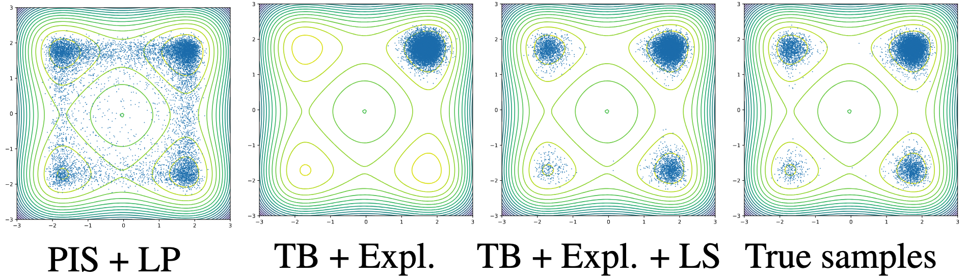
Figure 1: Two-dimensional projections of Manywell samples from models trained by different algorithms. Our proposed replay buffer with local search is capable of preventing mode collapse.

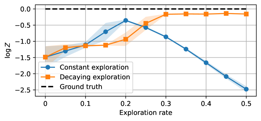
Figure 2: Effect of exploration variance on models trained with TB on the 25GMM energy. Exploration promotes mode discovery, but should be decayed over time to optimally allocate the modeling power to high-likelihood trajectories.

Benchmarking metrics.

To evaluate diffusion-based samplers, we use two metrics from past work (Zhang & Chen, 2022; Lahlou et al., 2023), which we restate in our notation. Given any forward policy $p_{F}$, we have a variational lower bound on the log-partition function $\log Z=\int_{{\mathbb{R}}^{d}}R({\mathbf{x}})\,d{\mathbf{x}}$:

$$\log\int_{{\mathbb{R}}^{d}}R({\mathbf{x}})\,d{\mathbf{x}} =\log{\mathbb{E}}_{\tau=(\dots\rightarrow{\mathbf{x}}_{1})\sim p_{F}(\tau)}\left[\frac{R({\mathbf{x}}_{1})p_{B}(\tau\mid{\mathbf{x}}_{1})}{p_{F}(\tau\mid{\mathbf{x}}_{1})}\right]$$

$$\geq{\mathbb{E}}_{\tau=(\dots\rightarrow{\mathbf{x}}_{1})\sim p_{F}(\tau)}\left[\log\frac{R({\mathbf{x}}_{1})p_{B}(\tau\mid{\mathbf{x}}_{1})}{p_{F}(\tau\mid{\mathbf{x}}_{1})}\right].$$

We use a $K$-sample Monte Carlo estimate of this expectation, $\log\hat{Z}$, as a metric, which always equals the true $\log Z$ if $p_{F}$ and $p_{B}$ jointly satisfy (10) and thus $p_{F}$ samples from the target distribution. (In our experiments, $K=2000$.)

We also employ an importance-weighted variant, which emphasizes mode coverage over accurate local modeling:

$$\log\hat{Z}^{\rm RW}:=\log\sum_{i=1}^{K}\left[\log\frac{R({\mathbf{x}}_{1}^{(i)})p_{B}(\tau^{(i)}\mid{\mathbf{x}}_{1}^{(i)})}{p_{F}(\tau^{(i)}\mid{\mathbf{x}}_{1}^{(i)})}\right],$$

where $\tau^{(1)},\dots,\tau^{(K)}$ are trajectories sampled from $p_{F}$ and leading to terminal states ${\mathbf{x}}_{1}^{(1)},\dots,{\mathbf{x}}_{1}^{(K)}$. The estimator $\log\hat{Z}^{\rm RW}$ is also a lower bound on $\log Z$ and approaches it as $K\to\infty$ (Burda et al., 2016). In the unconditional modeling benchmarks, we compare both estimators to the true log-partition function, which is known analytically.

In addition, we compute a sample-based metric, the squared 2-Wasserstein distance $\mathcal{W}_{2}^{2}$ between sets of $K$ samples from the true distribution and generated by a trained sampler.

5.2 Results

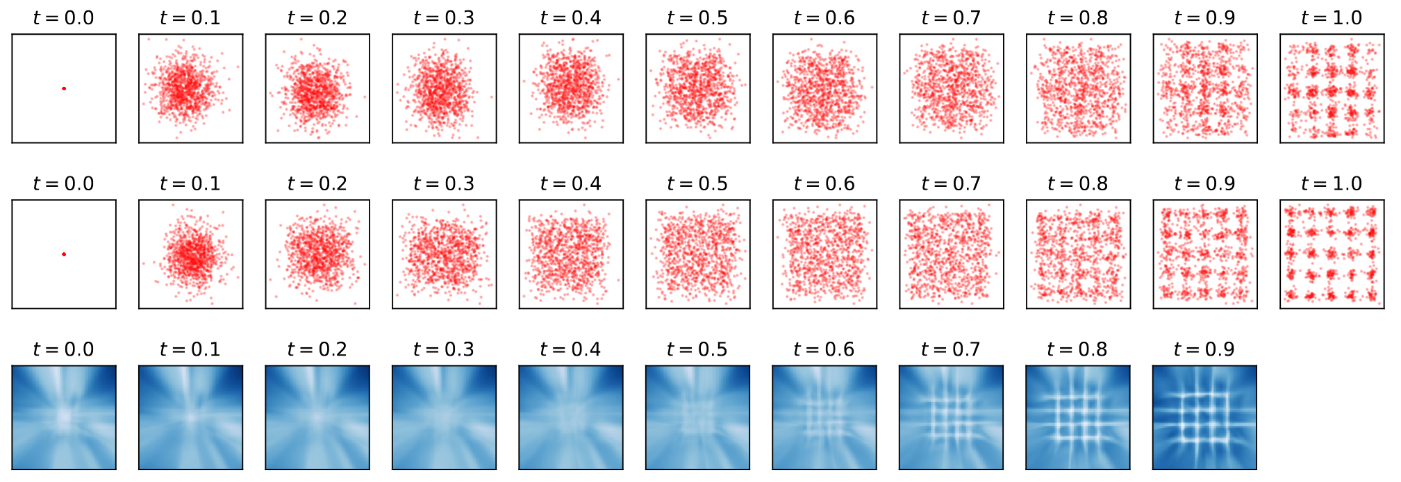
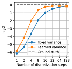
Figure 3: Left: Distribution of ${\mathbf{x}}_{0},{\mathbf{x}}_{0.1},\dots,{\mathbf{x}}_{1}$ learned by 10-step samplers with fixed (top) and learned (middle) forward policy variance on the 25GMM energy. The last step of sampling the fixed-variance model adds Gaussian noise of a variance close to that of the components of the target distribution, preventing the the sampler from sharply capturing the modes. The last row shows the policy variance learned as a function of ${\mathbf{x}}_{t}$ at various time steps $t$ (white is high variance, blue is low), showing that less noise is added around the peaks near $t=1$. The two models’ log-partition function estimates are $-1.67$ and $-0.62$, respectively. Right: For varying number of steps $T$, we plot the $\log\hat{Z}$ obtained by models with fixed and learned variance. Learning policy variances gives similar samplers with fewer steps.

Table 2: Log-likelihood estimates on a test set for a pretrained VAE decoder on MNIST. The latent being sampled is 20-dimensional. The VAE’s training ELBO (Gaussian encoder) was $\approx-101$.

Algorithm $\downarrow$ Metric $\rightarrow$	$\log\hat{Z}$	$\log\hat{Z}^{\rm RW}$
GGNS (Lemos et al., 2023)	$-82.406$$\pm 0.882$
PIS (Zhang & Chen, 2022)	$-102.54$$\pm 0.437$	$-47.753$$\pm 2.821$
+ LP (Zhang & Chen, 2022)	$-99.890$$\pm 0.373$	$-47.326$$\pm 0.777$
TB (Lahlou et al., 2023)	$-162.73$$\pm 35.55$	$-61.407$$\pm 17.83$
VarGrad	$-102.54$$\pm 0.934$	$-46.502$$\pm 1.018$
TB + Expl. (Lahlou et al., 2023)	$-148.04$$\pm 4.046$	$-49.967$$\pm 5.683$
FL-SubTB	$-202.78$$\pm 144.9$	$-67.501$$\pm 38.08$
+ LP (Zhang et al., 2024)	$-111.793$$\pm 0.704$	$-47.960$$\pm 1.121$
TB + Expl. + LS (ours)	$-245.78$$\pm 13.80$	$-55.378$$\pm 9.125$
TB + Expl. + LP (ours)	$-112.45$$\pm 0.671$	$-48.827$$\pm 1.787$
TB + Expl. + LP + LS (ours)	$-117.26$$\pm 2.502$	$-49.157$$\pm 2.051$
VarGrad + Expl. (ours)	$-103.39$$\pm 0.691$	$-47.318$$\pm 1.981$
VarGrad + Expl. + LS (ours)	$-105.40$$\pm 0.882$	$-48.235$$\pm 0.891$
VarGrad + Expl. + LP (ours)	$-99.472$$\pm 0.259$	$-46.574$$\pm 0.736$
VarGrad + Expl. + LP + LS (ours)	$-99.783$$\pm 0.312$	$-46.245$$\pm 0.543$

Unconditional sampling.

We report the metrics for all algorithms and energies in Table 1.

We observe that TB’s performance is generally modest without additional exploration and credit assignment mechanisms, except on the Funnel task, where variations in performance across methods are negligible. This confirms hypotheses from past work about the importance of off-policy exploration (Malkin et al., 2023; Lahlou et al., 2023) and the importance of improved credit assignment (Zhang et al., 2024). On the other hand, our results do not show a consistent and significant improvement of the FL-SubTB objective used by Zhang et al. (2024) over TB. Replacing TB with the VarGrad objective yields similar results.

The simple off-policy exploration method of adding variance to the policy notably enhances performance on the 25GMM task. We investigate this phenomenon in more detail in Fig. 2, finding that exploration that slowly decreases over the course of training is the best strategy.

On the other hand, our local search-guided exploration with a replay buffer (LS) leads to a substantial improvement in performance, surpassing or competing with GFlowNet baselines, non-GFlowNet baselines, and non-amortized sampling methods in most tasks and metrics. This advantage is attributed to efficient exploration and the ability to replay past low-energy regions, thus preventing mode collapse during training (Fig. 1). Further details on LS enhancements are discussed in §D with ablation studies in §D.2.

Incorporating Langevin parametrization (LP) into TB or FL-SubTB results in notable performance improvements (despite being 2-3$\times$ slower per iteration), indicating that the Zhang & Chen (2022)’s observations transfer to off-policy algorithms. Compared to FL-SubTB, which aims for enhanced credit assignment through partial energy, LP achieves superior credit assignment leveraging gradient information, akin to partial energy in continuous time. LP is either superior or competitive across most tasks and metrics.

Conditional sampling.

For the VAE task, we observe that the performance of the baseline GFlowNet-based samplers is generally worse than that of the simulation-based PIS (Table 2). While LP and LS improve the performance of TB, they do not close the gap in likelihood estimation; however, with the VarGrad objective, the performance is competitive with or superior to PIS. We hypothesize that this discrepancy is due to the difficulty of fitting the conditional log-partition function estimator, which is required for the TB objective but not for VarGrad, which only learns the policy. (In Fig. C.1 we show decoded samples encoded using the best-performing diffusion encoder.)

5.3 Extensions to general SDE learning problems

Our implementation of diffusion-structured generative flow networks includes several additional features that diverge from the modeling assumptions made in past work in the field. Notably, it features the ability to:

• optimize the backward (noising) process, not only the denoising process;

• learn the forward process’s diffusion rate $g({\mathbf{x}}_{t},t;\theta)$, not only the mean $u({\mathbf{x}}_{t},t;\theta)$;

• assume a varying noise schedule for the backward process, making it possible to train models with standard noising SDEs used for diffusion models for images.

These extensions will allow others to build on our implementation and apply it to problems such as finetuning diffusion models trained on images with a GFlowNet objective.

As noted in §5.1, in the main experiments we fixed the diffusion rate of the learned forward process, an assumption inherited from all past work and justified in the continuous-time limit. However, we perform an experiment to show the importance of extensions such as learning the forward variance in discrete time. Fig. 3 shows the samples of models on the 25GMM energy following the experimental setup of Lemos et al. (2023). We see that when the forward policy’s variance is learned, the model can better capture the details of the target distributions, choosing a low variance in the vicinity of the peaks to avoid ‘blurring’ them through the noise added in the last step of sampling.

The ability to model distributions accurately in fewer steps is important for computational efficiency. Future work can consider further extensions that improve performance in coarse time discretizations, such as non-Gaussian transition densities, whose utility in diffusion models trained from data has been demonstrated (Xiao et al., 2022).

6 Conclusion

We have presented a study of diffusion-structured samplers for amortized inference over continuous variables. Our results suggest promising techniques for improving the mode coverage and efficiency of these models. Future work on applications can consider inference of high-dimensional parameters of dynamical systems and inverse problems. In probabilistic machine learning, extensions of this work should study integration of our amortized sequential samplers as variational posteriors in an expectation-maximization loop for training latent variable models, as was recently done for discrete compositional latents by Hu et al. (2023), and for sampling Bayesian posteriors over high-dimensional model parameters. The most important direction of theoretical work is understanding the continuous-time limit ($T\to\infty$) of all the algorithms we have studied.

Impact statement

This work studies amortized variational inference over continuous variables, a problem of independent interest in Bayesian machine learning but also widely applicable in the sciences. We envision our work as a building block for future research in this field, setting necessary comparative standards amongst different methodologies and enabling fair benchmarking. We ultimately hope that our algorithms will be used responsibly and help to advance scientific understanding of the world.

Appendix A Code and hyperparameters

Code is available https://github.com/GFNOrg/gfn-diffusion and will continue to be maintained and extended.

Below are commands to reproduce some of the results on Manywell and VAE with PIS and GFlowNet models as an example, showing the hyperparameters:

PIS:

--mode_fwd pis  --lr_policy 1e-3

PIS + Langevin:

--mode_fwd pis  --lr_policy 1e-3 --langevin

GFlowNet TB:

python train.py
--t_scale 1. --energy many_well --pis_architectures --zero_init --clipping
--mode_fwd tb --lr_policy 1e-3 --lr_flow 1e-1

GFlowNet TB + Expl.:

python train.py
--t_scale 1. --energy many_well --pis_architectures --zero_init --clipping
--mode_fwd tb --lr_policy 1e-3 --lr_flow 1e-1
--exploratory --exploration_wd --exploration_factor 0.2

GFlowNet VarGrad + Expl.:

python train.py
--t_scale 1. --energy many_well --pis_architectures --zero_init --clipping
--mode_fwd tb-avg --lr_policy 1e-3 --lr_flow 1e-1
--exploratory --exploration_wd --exploration_factor 0.2

GFlowNet FL-SubTB:

python train.py
--t_scale 1. --energy many_well --pis_architectures --zero_init --clipping
--mode_fwd subtb --lr_policy 1e-3 --lr_flow 1e-2
--partial_energy --conditional_flow_model

GFlowNet FL-SubTB + LP:

python train.py
--t_scale 1. --energy many_well --pis_architectures --zero_init --clipping
--mode_fwd subtb --lr_policy 1e-3 --lr_flow 1e-2
--partial_energy --conditional_flow_model
--langevin --epochs 10000

GFlowNet TB + Expl. + LS:

python train.py
--t_scale 1. --energy many_well --pis_architectures --zero_init --clipping
--mode_fwd tb --lr_policy 1e-3 --lr_back 1e-3 --lr_flow 1e-1
--exploratory --exploration_wd --exploration_factor 0.1
--both_ways --local_search
--buffer_size 600000 --prioritized rank --rank_weight 0.01
--ld_step 0.1 --ld_schedule --target_acceptance_rate 0.574

GFlowNet TB + Expl. + LP:

python train.py
--t_scale 1. --energy many_well --pis_architectures --zero_init --clipping
--mode_fwd tb --lr_policy 1e-3 --lr_flow 1e-1
--exploratory --exploration_wd --exploration_factor 0.2
--langevin --epochs 10000

GFlowNet TB + Expl. + LS (VAE):

python train.py
--energy vae --pis_architectures --zero_init --clipping
--mode_fwd cond-tb-avg --mode_bwd cond-tb-avg --repeats 5
--lr_policy 1e-3 --lr_flow 1e-1 --lr_back 1e-3
--exploratory --exploration_wd --exploration_factor 0.1
--both_ways --local_search
--max_iter_ls 500 --burn_in 200
--buffer_size 90000 --prioritized rank --rank_weight 0.01
--ld_step 0.001 --ld_schedule --target_acceptance_rate 0.574

GFlowNet TB + Expl. + LP + LS (VAE):

python train.py
--energy vae --pis_architectures --zero_init --clipping
--mode_fwd cond-tb-avg --mode_bwd cond-tb-avg --repeats 5
--lr_policy 1e-3 --lr_flow 1e-1
--lgv_clip 1e2 --gfn_clip 1e4 --epochs 10000
--exploratory --exploration_wd --exploration_factor 0.1
--both_ways --local_search
--lr_back 1e-3 --max_iter_ls 500 --burn_in 200
--buffer_size 90000 --prioritized rank  --rank_weight 0.01
--langevin
--ld_step 0.001 --ld_schedule --target_acceptance_rate 0.574

Appendix B Target densities

Gaussian Mixture Model with 25 modes (25GMM). The model, termed as $25\mathrm{GMM}$, consists of a two-dimensional Gaussian mixture model with 25 distinct modes. Each mode exhibits an identical variance of $0.3$. The centers of these modes are strategically positioned on a grid formed by the Cartesian product $\{-10,-5,0,5,10\}\times\{-10,-5,0,5,10\}$, effectively distributing them across the coordinate space.

Funnel (Hoffman et al., 2019). The funnel represents a classical benchmark in sampling techniques, characterized by a ten-dimensional distribution defined as follows: The first dimension, $x_{0}$, follows a normal distribution with mean $0$ and variance $9$, denoted as $x_{0}\sim\mathcal{N}(0,9)$. Conditional on $x_{0}$, the remaining dimensions, $x_{1:9}$, are distributed according to a multivariate normal distribution with mean vector $\mathbf{0}$ and a covariance matrix $\exp(x_{0})\mathbf{I}$, where $\mathbf{I}$ is the identity matrix. This is succinctly represented as $x_{1:9}\mid x_{0}\sim\mathcal{N}\left(\mathbf{0},\exp\left(x_{0}\right)\mathbf{I}\right)$.

Manywell (Noé et al., 2019). The manywell is characterized by a 32-dimensional distribution, which is constructed as the product of 16 identical two-dimensional double well distributions. Each of these two-dimensional components is defined by a potential function, $\mu(x_{1},x_{2})$, expressed as $\mu(x_{1},x_{2})=\exp\left(-x_{1}^{4}+6x_{1}^{2}+0.5x_{1}-0.5x_{2}^{2}\right)$.

VAE (Kingma & Welling, 2014). This task involves sampling from a 20-dimensional latent posterior $p(z|x)\propto p(z)p(x|z)$, where $p(z)$ is a fixed prior and $p(x|z)$ is a pretrained VAE decoder, using a conditional sampler $q(z|x)$ dependent on input data (image) $x$.

Appendix C Experiment details

Sampling energies.

In this section, we detail the hyperparameters used for our experiments. An important parameter is the diffusion coefficient of the forward policy, which is denoted by $\sigma$ and also used in the definition of the fixed backward process. The base diffusion rate $\sigma^{2}$ (parameter t_scale) is set to 5 for 25GMM and 1 for Funnel and Manywell, consistent with past work.

For all our experiments, we used a learning rate of $10^{-3}$. Additionally, we used a higher learning rate for learning the flow parameterization, which is set as $10^{-1}$ when using the TB loss and $10^{-2}$ with the SubTB loss. These settings were found to be consistently stable (unlike those with higher learning rates) and converge within the allotted number of steps (unlike those with lower learning rates).

For the SubTB loss, we experimented with the settings of $10\times$ lower learning rates for both flow and policy models communicated by the authors of Zhang et al. (2024), but found the results to be inferior both using their published code (and other unstated hyperparameters communicated by the authors) and using our reimplementation.

For models with exploration, we use an exploration factor of $0.2$ (that is, noise with a variance of 0.2 is added to the policy when sampling trajectories for training), which decays linearly over the first half of training, consistent with Lahlou et al. (2023).

We train all our models for $25,000$ iterations except those using Langevin dynamics, which are trained for $10,000$ iterations. This results in approximately equal computation time owing to the overhead from computation of the score at each sampling step.

We use the same neural network architecture for the GFlowNet as one of our baselines (Zhang & Chen, 2022). Similar to Zhang & Chen (2022), we also use an initialization scheme with last-layer weights set to 0 at the start of training. Since the SubTB requires the flow function to be conditioned on the current state ${\mathbf{x}}_{t}$ and time $t$, we follow Zhang et al. (2024) and parametrize the flow model with the same architecture as the Langevin scaling model ${\rm NN}_{2}$ in Zhang & Chen (2022). Additionally, we perform clipping on the output of the network as well as the score obtained from the energy function, typically setting the clipping parameter of Langevin scaling model to $10^{2}$ and policy network to $10^{4}$, similarly to Vargas et al. (2023):

$$f_{\theta}(k,x)\!=\!{\color[rgb]{0,0,1}\mathrm{clip}\Big{(}}\mathrm{NN}_{1}(k,x;\theta)+\mathrm{NN}_{2}(k;\theta)\odot{\color[rgb]{1,0,0}\mathrm{clip}}{\color[rgb]{1,0,0}\big{(}}\nabla\ln\pi(x){\color[rgb]{1,0,0},-10^{2},10^{2}\big{)}}{\color[rgb]{0,0,1},-10^{4},10^{4}\Big{)}}.$$ (16)

All models were trained with a batch size of 300.

VAE experiment.

In the VAE experiment, we used a standard VAE model pretrained for 100 epochs on the MNIST dataset. The encoder $q(z|x)$ contains an input linear layer (784 neurons) followed by hidden linear layer (400 neurons), ReLU activation function, and two linear heads (20 neurons each) whose outputs were reparametrized to be means and scales of multivariate Normal distribution. The decoder consists of 20-dimensional input, one hidden layer (400 neurons), followed by the ReLU activation, and 784-dimensional output. The output is processed by the sigmoid function to be scaled properly into $[0,1]$.

The goal is to sample conditionally on $x$ the latent $z$ from the unnormalized density $p(z,x)=p(z)p(x\mid z)$ (where $p(z)$ is the prior and $p(x|z)$ is the likelihood computed from the decoder), which is proportional to the posterior $p(z\mid x)$. We reuse the model architectures from the unconditional sampling experiments, but also provide $x$ as an input to the first layer of the models expressing the policy drift (as well as the flow, for FL-SubTB) and add one hidden layer to process high-dimensional conditions. For models trained with TB, $\log Z_{\theta}$ also becomes a MLP taking $x$ as input.

The VarGrad and LS techniques require adaptations in the conditional setting. For LS, buffers ($\mathcal{D}_{\text{buffer}}$ and $\mathcal{D}_{\text{LS}}$) must store the associated conditions $x$ together with the samples $z$ and the corresponding unnormalized density $R(z;x)$, i.e., a tuple of $(x,z,R(z;x))$. For VarGrad, because the partition function depends on the conditioning information $x$, it is necessary to compute variance over many trajectories sharing the same condition. We choose to sample 10 trajectories for each condition occurring in a minibatch and compute the VarGrad loss for each such set of 10 trajectories.

The VAE model was trained on the entire MNIST training set and never updated on the test part of MNIST. In order to evaluate samplers (with respect to the variational lower bound) on a unique set of examples, we chose the first 100 elements of MNIST test data. All of the samplers were trained having access to the MNIST training data and the frozen VAE decoder. For a fair comparison, samplers utilizing the LP were trained for $10,000$, whereas the remaining for $25,000$ iterations. In each iteration, a batch of 300 examples from MNIST was given as conditions.

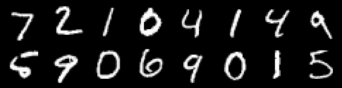
(a) Conditioning data (MNIST test set)

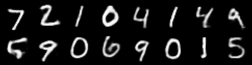
(b) VarGrad + Expl. + LP samples decoded

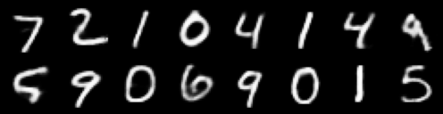
(c) VAE reconstruction

Figure C.1: Our sampler (VarGrad + Expl. + LP) is conditioned by a subset of never-seen data coming from the ground truth distribution (left). The conditional samples were then decoded by the the fixed VAE (middle). For the comparison, we show the reconstruction of the real data by VAE (right). We observed that the decoded samples are visually very similar to the reconstructions making these two pictures almost indistinguishable. Both, decoded samples and reconstruction, are more blurry than the ground truth data, which is caused by a limited capacity of the VAE’s latent space.

Appendix D Local search-guided GFlowNet

Prioritized sampling scheme.

We can use uniform or prioritized sampling to draw samples from the buffer for training. We found prioritized sampling to work slightly better in our experiments (see ablation study in §D.2), although the choice should be investigated more thoroughly in future work.

We use rank-based prioritization (Tripp et al., 2020), which follows a probabilistic approach defined as:

$$p({\mathbf{x}};\mathcal{D}_{\text{buffer}})\propto\left(k|\mathcal{D}_{\text{buffer}}|+\text{rank}_{\mathcal{D}_{\text{buffer}}}({\mathbf{x}})\right)^{-1},$$ (17)

where $\text{rank}_{\mathcal{D}_{\text{buffer}}}({\mathbf{x}})$ represents the relative rank of a sample $x$ based on a ranking function $R({\mathbf{x}})$ (in our case, the unnormalized target density at sample ${\mathbf{x}}$). The parameter $k$ is a hyperparameter for prioritization, where a lower value of $k$ assigns a higher probability to samples with higher ranks, thereby introducing a more greedy selection approach. We set $k=0.01$ for every task. Given that the sampling is proportional to the size of $\mathcal{D}_{\text{buffer}}$, we impose a constraint on the maximum size of the buffer: $|\mathcal{D}_{\text{buffer}}|=600,000$ with first-in first out (FIFO) data structure for every task, except we use $|\mathcal{D}_{\text{buffer}}|=90,000$ for VAE task. See the algorithm below for a detailed pseudocode.

Algorithm 1 GFlowNet Training with Local search

1:  Initialize policy parameters $\theta$ for $P_{F}$, and empty buffers $\mathcal{D}_{\text{buffer}},\mathcal{D}_{\text{LS}}$

2:  for $i=1,2,\ldots,I$ do

3:    if $i\%2==0$ then

4:       Sample $M$ trajectories $\{\tau_{1},\ldots,\tau_{M}\}\sim P_{F}(\cdot|\epsilon\text{-greedy})$

5:       Update $\mathcal{D}_{\text{buffer}}\leftarrow\mathcal{D}_{\text{buffer}}\cup\{x|\tau\rightarrow x\}$

6:       Minimize $L(\tau;\theta)$ using $\{\tau_{1},\ldots,\tau_{M}\}$ to update $P_{F}$

7:    else

8:       if $i\%100==0$ then

9:          Sample $\{x_{1},\ldots,x_{M}\}\sim\mathcal{D}_{\text{buffer}}$

10:          $\mathcal{D}_{\text{LS}}\leftarrow\text{Local Search}(\{x_{1},\ldots,x_{M}\};\mathcal{D}_{\text{LS}})$

11:       end if

12:       Sample $\{x^{\prime}_{1},\ldots,x^{\prime}_{M}\}\sim p_{\text{buffer}}(\cdots;\mathcal{D}_{\text{LS}})$

13:       Sample $\{\tau^{\prime}_{1},\ldots,\tau^{\prime}_{M}\}\sim P_{B}(\cdots|x^{\prime})$

14:       Minimize $L(\tau^{\prime};\theta)$ using $\{\tau^{\prime}_{1},\ldots,\tau^{\prime}_{M}\}$ to update $P_{F}$

15:    end if

16:  end for

We use the number of total iterations $I=25,000$ for every task as default. Note as local search is performed to update $\mathcal{D}_{\text{LS}}$ occasionally that per $100$ iterations, the number of local search updates is done $25,000/100=250$.

D.1 Local search algorithm

This section describes a detailed algorithm for local search, which provides an updated buffer $\mathcal{D}_{\text{LS}}$, which contains low-energy samples.

Dynamic adjustment of step size $\eta$.

To enhance local search using parallel MALA, we dynamically select the Langevin step size ($\eta$), which governs the MH acceptance rate. Our objective is to attain an average acceptance rate of 0.574, which is theoretically optimal for high-dimensional MALA’s efficiency (Pillai et al., 2012). While the user can customize the target acceptance rate, the adaptive approach eliminates the need for manual tuning.

Computational cost of local search.

The computational cost of local search is not significant. Local search for iteration of $K=200$ requires $6.04$ seconds (averaged with five trials in Manywell), where we only occasionally (every 100 iterations) update ${\mathcal{D}}_{\text{LS}}$ with MALA. The speed is evaluated using the computational resources of the Intel Xeon Scalable Gold 6338 CPU (2.00GHz) and the NVIDIA RTX 4090 GPU.

Algorithm 2 Local search (Parallel MALA)

0:  Initial states $\{x_{1}^{(0)},\ldots,x_{M}^{(0)}\}$, current buffer $\mathcal{D}_{\text{LS}}$, total steps $K$, burn in steps $K_{\text{burn-in}}$, initial step size $\eta_{0}$, amplifying factor $f_{\text{increase}}$, damping factor $f_{\text{decrease}}$, unnormalized target density $R$

0:  Updated buffer $\mathcal{D}_{\text{LS}}$

  Initialize acceptance counter $a=0$

  Set $\eta\leftarrow\eta_{0}$

  for $k=1:K$ do

    Initialize step acceptance count $a_{k}=0$

    for $m=1:M$ do

       Sample $\sigma\sim\mathcal{N}(0,I)$

       Propose $x_{m}^{*}\leftarrow x_{m}^{(k-1)}+\eta\nabla\log R(x_{m}^{(k-1)})+\sqrt{2\eta}\sigma$

       Compute acceptance ratio $r\leftarrow\min\left(1,\frac{R(x_{m}^{*})\exp\left(-\frac{1}{4\eta}\|x_{m}^{(k-1)}-x_{m}^{*}-\eta\nabla\log R(x_{m}^{*})\|^{2}\right)}{R(x_{m}^{(k-1)})\exp\left(-\frac{1}{4\eta}\|x_{m}^{*}-x_{m}^{(k-1)}-\eta\nabla\log R(x_{m}^{(k-1)})\|^{2}\right)}\right)$

       With probability $r$, accept the proposal: $x_{m}^{(k)}\leftarrow x_{m}^{*}$ and increment $a_{k}\leftarrow a_{k}+1$

       if $k>K_{\text{burn-in}}$ then

          Update buffer: $\mathcal{D}_{\text{LS}}\leftarrow\mathcal{D}_{\text{LS}}\cup\{x^{*}_{m}\}$

       end if

    end for

    Compute step acceptance rate $\alpha_{k}=a_{k}/M$

    if $\alpha_{k}>\alpha_{\text{target}}$ then

       $\eta\leftarrow\eta\times f_{\text{increase}}$

    else if $\alpha_{k}<\alpha_{\text{target}}$ then

       $\eta\leftarrow\eta\times f_{\text{decrease}}$

    end if

  end for

We adopt default parameters: $f_{\text{increase}}=1.1$, $f_{\text{decrease}}=0.9$, $\eta_{0}=0.01$, $K=200$, $K_{\text{burn-in}}=100$, and $\alpha_{\text{target}}=0.574$ for three unconditional tasks. For conditional tasks of VAE, we give more iterations of local search: $K=500$, $K_{\text{burn-in}}=200$.

It is noteworthy that by adjusting the inverse temperature $\beta$ into $R^{\beta}$ during the computation of the Metropolis-Hastings acceptance ratio $r$, we can facilitate a greedier local search strategy aimed at exploring samples with lower energy (i.e., higher density $p_{\rm target}$). This approach proves advantageous for navigating high-dimensional and steep landscapes, which are typically challenging for locating low-energy samples. For unconditional tasks, we set $\beta=1$.

In the context of the VAE task (Table 2), we utilize two GFlowNet loss functions: TB and VarGrad. For local search within TB, we set $\beta=1$, while for VarGrad, we employ $\beta=5$. As illustrated in Table 2, employing a local search with $\beta=1$ fails to enhance the performance of the TB method. Conversely, a local search with $\beta=5$ results in improvements at the $\log\hat{Z}^{\text{RW}}$ metric over the VarGrad + Expl. + LP, even though the performance of VarGrad + Expl. + LP surpasses that of TB substantially. This underscores the importance of selecting an appropriate $\beta$ value, which is critical for optimizing the exploration-exploitation balance depending on the target objectives.

D.2 Ablation study for local search-guided GFlowNets

Increasing capacity of buffer.

The capacity of the replay buffer influences the duration for which it retains past experiences, enabling it to replay these experiences to the policy. This mechanism helps in preventing mode collapse during training. Table D.1 demonstrates that enhancing the buffer’s capacity leads to improved sampling quality. Furthermore, Figure 1 illustrates that increasing the buffer’s capacity—thereby encouraging the model to recall past low-energy experiences—enhances its mode-seeking capability.

Table D.1: Comparison of the sampling quality of each sampler trained with varying replay buffer capacities in Manywell. Five independent runs have been conducted, with both the mean and standard deviation reported.

Buffer Capacity $\downarrow$ Metric $\rightarrow$	$\Delta\log Z$	$\Delta\log Z^{\rm RW}$	$\mathcal{W}_{2}^{2}$
$30,000$	$4.41$$\pm 0.10$	$2.73$$\pm 0.15$	$6.17$$\pm 0.02$
$60,000$	$4.06$$\pm 0.05$	$2.38$$\pm 0.38$	$6.14$$\pm 0.04$
$600,000$	4.57$\pm 2.13$	0.19$\pm 0.29$	5.66$\pm 0.05$

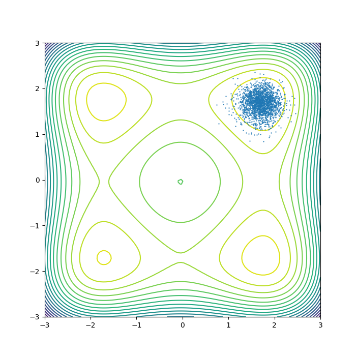
(a) Capacity $30,000$

(b) Capacity $60,000$

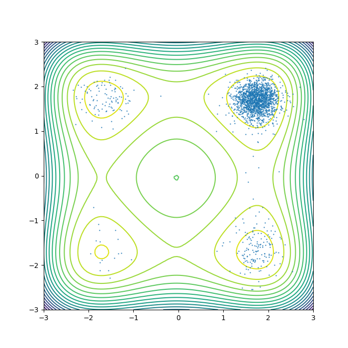
(c) Capacity $600,000$

Figure D.1: Illustration of each sampler trained with varying capacities of replay buffers, depicting 2,000 samples. As the capacity of the buffer increases, the number of modes captured by the sampler also increases.

Benefit of prioritization.

Rank-prioritized sampling gives faster convergence compared with no prioritization (uniform sampling), as shown in Fig. D.2.

Dynamic adjustment of $\eta$ vs. fixed $\eta=0.01$.

As shown in Fig. D.2, dynamic adjustment to target acceptance rate $\alpha_{\text{target}}=0.574$ gives better performances than fixed Langevin step size of $\eta$ showcasing the effectiveness of the dynamic adjustment.

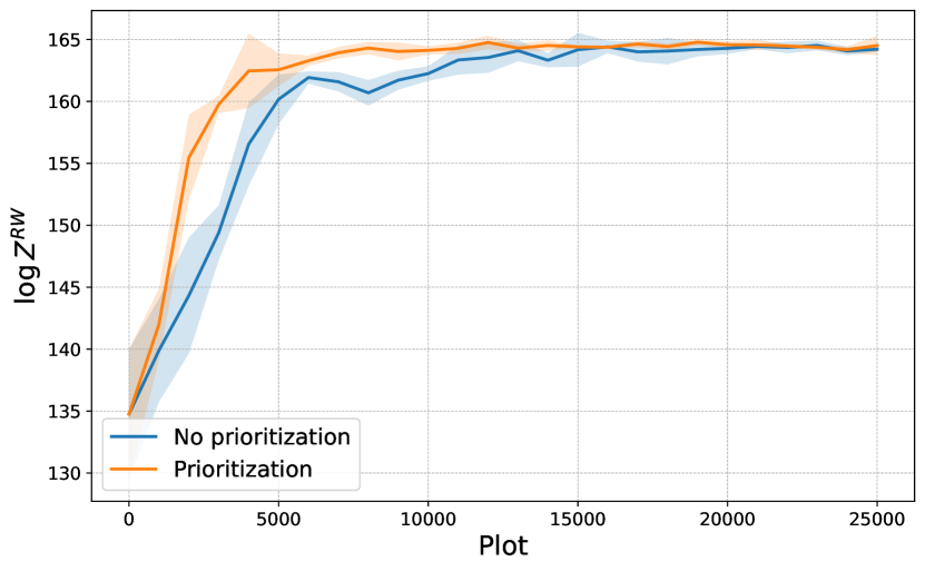
(a) Benefit of prioritization in replay buffer sampling..

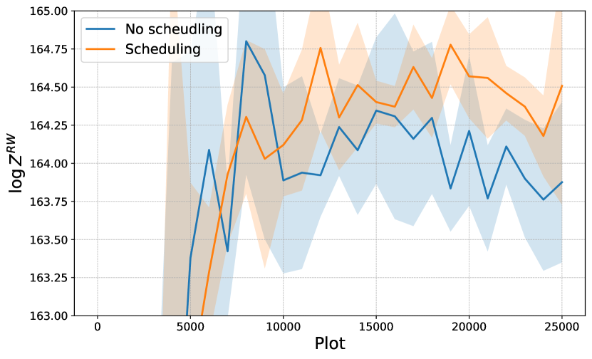
(b) Benefit of scheduling $\eta$ dynamically.

Figure D.2: Ablation study for prioritized replay buffer and step size $\eta$ scheduling of local search. Mean and standard deviation are plotted based on five independent runs.

References

- Adam et al. (2022) Adam, A., Coogan, A., Malkin, N., Legin, R., Perreault-Levasseur, L., Hezaveh, Y., and Bengio, Y. Posterior samples of source galaxies in strong gravitational lenses with score-based priors. arXiv preprint arXiv:2211.03812, 2022.
- Agrawal & Domke (2021) Agrawal, A. and Domke, J. Amortized variational inference for simple hierarchical models. Neural Information Processing Systems (NeurIPS), 2021.
- Albergo et al. (2019) Albergo, M. S., Kanwar, G., and Shanahan, P. E. Flow-based generative models for Markov chain Monte Carlo in lattice field theory. Physical Review D, 100(3):034515, 2019.
- Atanackovic et al. (2023) Atanackovic, L., Tong, A., Wang, B., Lee, L. J., Bengio, Y., and Hartford, J. DynGFN: Towards bayesian inference of gene regulatory networks with GFlowNets. Neural Information Processing Systems (NeurIPS), 2023.
- Bandeira et al. (2022) Bandeira, A. S., Maillard, A., Nickl, R., and Wang, S. On free energy barriers in Gaussian priors and failure of cold start MCMC for high-dimensional unimodal distributions. Philosophical transactions. Series A, Mathematical, physical, and engineering sciences, 381, 2022.
- Bengio et al. (2021) Bengio, E., Jain, M., Korablyov, M., Precup, D., and Bengio, Y. Flow network based generative models for non-iterative diverse candidate generation. Neural Information Processing Systems (NeurIPS), 2021.
- Bengio et al. (2023) Bengio, Y., Lahlou, S., Deleu, T., Hu, E. J., Tiwari, M., and Bengio, E. GFlowNet foundations. Journal of Machine Learning Research, 24(210):1–55, 2023.
- Berner et al. (2022) Berner, J., Richter, L., and Ullrich, K. An optimal control perspective on diffusion-based generative modeling. arXiv preprint arXiv:2211.01364, 2022.
- Buchner (2021) Buchner, J. Nested sampling methods. arXiv preprint arXiv:2101.09675, 2021.
- Burda et al. (2016) Burda, Y., Grosse, R. B., and Salakhutdinov, R. Importance weighted autoencoders. International Conference on Learning Representations (ICLR), 2016.
- Chopin (2002) Chopin, N. A sequential particle filter method for static models. Biometrika, 89(3):539–552, 2002.
- Cornish et al. (2020) Cornish, R., Caterini, A., Deligiannidis, G., and Doucet, A. Relaxing bijectivity constraints with continuously indexed normalising flows. International Conference on Machine Learning (ICML), 2020.
- De Bortoli (2022) De Bortoli, V. Convergence of denoising diffusion models under the manifold hypothesis. Transactions on Machine Learning Research (TMLR), 2022.
- Del Moral et al. (2006) Del Moral, P., Doucet, A., and Jasra, A. Sequential Monte Carlo samplers. Journal of the Royal Statistical Society Series B: Statistical Methodology, 68(3):411–436, 2006.
- Deleu et al. (2022) Deleu, T., Góis, A., Emezue, C., Rankawat, M., Lacoste-Julien, S., Bauer, S., and Bengio, Y. Bayesian structure learning with generative flow networks. Uncertainty in Artificial Intelligence (UAI), 2022.
- Dinh et al. (2017) Dinh, L., Sohl-Dickstein, J., and Bengio, S. Density estimation using Real NVP. International Conference on Learning Representations (ICLR), 2017.
- Duane et al. (1987) Duane, S., Kennedy, A., Pendleton, B. J., and Roweth, D. Hybrid Monte Carlo. Physics Letters B, 195(2):216–222, 1987.
- Gao et al. (2020) Gao, C., Isaacson, J., and Krause, C. i-flow: High-dimensional integration and sampling with normalizing flows. Machine Learning: Science and Technology, 1(4):045023, 2020.
- Grathwohl et al. (2019) Grathwohl, W., Chen, R. T., Bettencourt, J., Sutskever, I., and Duvenaud, D. FFJORD: Free-form continuous dynamics for scalable reversible generative models. International Conference on Learning Representations (ICLR), 2019.
- Grenander & Miller (1994) Grenander, U. and Miller, M. I. Representations of knowledge in complex systems. Journal of the Royal Statistical Society: Series B (Methodological), 56(4):549–581, 1994.
- Halton (1962) Halton, J. H. Sequential Monte Carlo. In Mathematical Proceedings of the Cambridge Philosophical Society, volume 58, pp. 57–78. Cambridge University Press, 1962.
- Harrison et al. (2024) Harrison, J., Willes, J., and Snoek, J. Variational Bayesian last layers. International Conference on Learning Representations (ICLR), 2024.
- Hernández-Lobato & Adams (2015) Hernández-Lobato, J. M. and Adams, R. Probabilistic backpropagation for scalable learning of Bayesian neural networks. International Conference on Machine Learning (ICML), 2015.
- Ho et al. (2020) Ho, J., Jain, A., and Abbeel, P. Denoising diffusion probabilistic models. Neural Information Processing Systems (NeurIPS), 2020.
- Hoffman et al. (2019) Hoffman, M., Sountsov, P., Dillon, J. V., Langmore, I., Tran, D., and Vasudevan, S. NeuTra-lizing bad geometry in Hamiltonian Monte Carlo using neural transport. arXiv preprint arXiv:1903.03704, 2019.
- Hoffman et al. (2013) Hoffman, M. D., Blei, D. M., Wang, C., and Paisley, J. W. Stochastic variational inference. Journal of Machine Learning Research (JMLR), 14:1303–1347, 2013.
- Hoffman et al. (2014) Hoffman, M. D., Gelman, A., et al. The No-U-Turn sampler: adaptively setting path lengths in Hamiltonian Monte Carlo. Journal of Machine Learning Research (JMLR), 15(1):1593–1623, 2014.
- Holdijk et al. (2023) Holdijk, L., Du, Y., Hooft, F., Jaini, P., Ensing, B., and Welling, M. Stochastic optimal control for collective variable free sampling of molecular transition paths. Neural Information Processing Systems (NeurIPS), 2023.
- Hu et al. (2023) Hu, E. J., Malkin, N., Jain, M., Everett, K., Graikos, A., and Bengio, Y. GFlowNet-EM for learning compositional latent variable models. International Conference on Machine Learning (ICML), 2023.
- Hu et al. (2024) Hu, E. J., Jain, M., Elmoznino, E., Kaddar, Y., Lajoie, G., Bengio, Y., and Malkin, N. Amortizing intractable inference in large language models. International Conference on Learning Representations (ICLR), 2024.
- Izmailov et al. (2021) Izmailov, P., Vikram, S., Hoffman, M. D., and Wilson, A. G. What are Bayesian neural network posteriors really like? International Conference on Machine Learning (ICML), 2021.
- Jain et al. (2022) Jain, M., Bengio, E., Hernandez-Garcia, A., Rector-Brooks, J., Dossou, B. F., Ekbote, C. A., Fu, J., Zhang, T., Kilgour, M., Zhang, D., et al. Biological sequence design with gflownets. International Conference on Machine Learning (ICML), 2022.
- Jang et al. (2024) Jang, H., Kim, M., and Ahn, S. Learning energy decompositions for partial inference of GFlowNets. International Conference on Learning Representations (ICLR), 2024.
- Jing et al. (2022) Jing, B., Corso, G., Chang, J., Barzilay, R., and Jaakkola, T. Torsional diffusion for molecular conformer generation. Neural Information Processing Systems (NeurIPS), 2022.
- Kim et al. (2023) Kim, M., Ko, J., Zhang, D., Pan, L., Yun, T., Kim, W., Park, J., and Bengio, Y. Learning to scale logits for temperature-conditional GFlowNets. arXiv preprint arXiv:2310.02823, 2023.
- Kim et al. (2024) Kim, M., Yun, T., Bengio, E., Zhang, D., Bengio, Y., Ahn, S., and Park, J. Local search GFlowNets. International Conference on Learning Representations (ICLR), 2024.
- Kingma & Welling (2014) Kingma, D. P. and Welling, M. Auto-encoding variational Bayes. International Conference on Learning Representations (ICLR), 2014.
- Lahlou et al. (2023) Lahlou, S., Deleu, T., Lemos, P., Zhang, D., Volokhova, A., Hernández-Garcıa, A., Ezzine, L. N., Bengio, Y., and Malkin, N. A theory of continuous generative flow networks. International Conference on Machine Learning (ICML), 2023.
- Lemos et al. (2023) Lemos, P., Malkin, N., Handley, W., Bengio, Y., Hezaveh, Y., and Perreault-Levasseur, L. Improving gradient-guided nested sampling for posterior inference. arXiv preprint arXiv:2312.03911, 2023.
- Madan et al. (2022) Madan, K., Rector-Brooks, J., Korablyov, M., Bengio, E., Jain, M., Nica, A., Bosc, T., Bengio, Y., and Malkin, N. Learning GFlowNets from partial episodes for improved convergence and stability. International Conference on Machine Learning (ICML), 2022.
- Malkin et al. (2022) Malkin, N., Jain, M., Bengio, E., Sun, C., and Bengio, Y. Trajectory balance: Improved credit assignment in gflownets. Neural Information Processing Systems (NeurIPS), 2022.
- Malkin et al. (2023) Malkin, N., Lahlou, S., Deleu, T., Ji, X., Hu, E., Everett, K., Zhang, D., and Bengio, Y. GFlowNets and variational inference. International Conference on Learning Representations (ICLR), 2023.
- Máté & Fleuret (2023) Máté, B. and Fleuret, F. Learning interpolations between Boltzmann densities. Transactions on Machine Learning Research (TMLR), 2023.
- Nichol & Dhariwal (2021) Nichol, A. and Dhariwal, P. Improved denoising diffusion probabili1stic models. International Conference on Machine Learning (ICML), 2021.
- Nicoli et al. (2020) Nicoli, K. A., Nakajima, S., Strodthoff, N., Samek, W., Müller, K.-R., and Kessel, P. Asymptotically unbiased estimation of physical observables with neural samplers. Physical Review E, 101(2):023304, 2020.
- Noé et al. (2019) Noé, F., Olsson, S., Köhler, J., and Wu, H. Boltzmann generators: Sampling equilibrium states of many-body systems with deep learning. Science, 365(6457):eaaw1147, 2019.
- Øksendal (2003) Øksendal, B. Stochastic Differential Equations: An Introduction with Applications. Springer, 2003.
- Pan et al. (2023) Pan, L., Malkin, N., Zhang, D., and Bengio, Y. Better training of GFlowNets with local credit and incomplete trajectories. International Conference on Machine Learning (ICML), 2023.
- Pillai et al. (2012) Pillai, N. S., Stuart, A. M., and Thiéry, A. H. Optimal scaling and diffusion limits for the langevin algorithm in high dimensions. The Annals of Applied Probability, 22(6), December 2012.
- Ranganath et al. (2014) Ranganath, R., Gerrish, S., and Blei, D. Black box variational inference. Artificial Intelligence and Statistics (AISTATS), 2014.
- Rector-Brooks et al. (2023) Rector-Brooks, J., Madan, K., Jain, M., Korablyov, M., Liu, C.-H., Chandar, S., Malkin, N., and Bengio, Y. Thompson sampling for improved exploration in GFlowNets. arXiv preprint arXiv:2306.17693, 2023.
- Rezende & Mohamed (2015) Rezende, D. and Mohamed, S. Variational inference with normalizing flows. International Conference on Machine Learning (ICML), 2015.
- Rezende et al. (2014) Rezende, D. J., Mohamed, S., and Wierstra, D. Stochastic backpropagation and approximate inference in deep generative models. International Conference on Machine Learning (ICML), 2014.
- Richter et al. (2020) Richter, L., Boustati, A., Nüsken, N., Ruiz, F. J. R., and Ömer Deniz Akyildiz. VarGrad: A low-variance gradient estimator for variational inference. Neural Information Processing Systems (NeurIPS), 2020.
- Richter et al. (2023) Richter, L., Berner, J., and Liu, G.-H. Improved sampling via learned diffusions. International Conference on Learning Representations (ICLR), 2023.
- Roberts & Rosenthal (1998) Roberts, G. O. and Rosenthal, J. S. Optimal scaling of discrete approximations to langevin diffusions. Journal of the Royal Statistical Society: Series B (Statistical Methodology), 60(1):255–268, 1998.
- Roberts & Tweedie (1996) Roberts, G. O. and Tweedie, R. L. Exponential convergence of Langevin distributions and their discrete approximations. Bernoulli, pp. 341–363, 1996.
- Rombach et al. (2021) Rombach, R., Blattmann, A., Lorenz, D., Esser, P., and Ommer, B. High-resolution image synthesis with latent diffusion models. Conference on Computer Vision and Pattern Recognition (CVPR), 2021.
- Särkkä & Solin (2019) Särkkä, S. and Solin, A. Applied stochastic differential equations. Cambridge University Press, 2019.
- Shen et al. (2023) Shen, M. W., Bengio, E., Hajiramezanali, E., Loukas, A., Cho, K., and Biancalani, T. Towards understanding and improving GFlowNet training. International Conference on Machine Learning (ICML), 2023.
- Skilling (2006) Skilling, J. Nested sampling for general Bayesian computation. Bayesian Analysis, 1(4):833 – 859, 2006. doi: 10.1214/06-BA127. URL https://doi.org/10.1214/06-BA127.
- Sohl-Dickstein et al. (2015) Sohl-Dickstein, J., Weiss, E. A., Maheswaranathan, N., and Ganguli, S. Deep unsupervised learning using nonequilibrium thermodynamics. International Conference on Machine Learning (ICML), 2015.
- Song et al. (2021a) Song, Y., Durkan, C., Murray, I., and Ermon, S. Maximum likelihood training of score-based diffusion models. Neural Information Processing Systems (NeurIPS), 2021a.
- Song et al. (2021b) Song, Y., Sohl-Dickstein, J., Kingma, D. P., Kumar, A., Ermon, S., and Poole, B. Score-based generative modeling through stochastic differential equations. International Conference on Learning Representations (ICLR), 2021b.
- Tiapkin et al. (2023) Tiapkin, D., Morozov, N., Naumov, A., and Vetrov, D. Generative flow networks as entropy-regularized RL. arXiv preprint arXiv:2310.12934, 2023.
- Tripp et al. (2020) Tripp, A., Daxberger, E., and Hernández-Lobato, J. M. Sample-efficient optimization in the latent space of deep generative models via weighted retraining. Neural Information Processing Systems (NeurIPS), 2020.
- Tzen & Raginsky (2019a) Tzen, B. and Raginsky, M. Neural stochastic differential equations: Deep latent Gaussian models in the diffusion limit. arXiv preprint arXiv:1905.09883, 2019a.
- Tzen & Raginsky (2019b) Tzen, B. and Raginsky, M. Theoretical guarantees for sampling and inference in generative models with latent diffusions. Conference on Learning Theory (CoLT), 2019b.
- van Krieken et al. (2023) van Krieken, E., Thanapalasingam, T., Tomczak, J., van Harmelen, F., and ten Teije, A. A-NeSI: A scalable approximate method for probabilistic neurosymbolic inference. Neural Information Processing Systems (NeurIPS), 2023.
- Vargas et al. (2023) Vargas, F., Grathwohl, W., and Doucet, A. Denoising diffusion samplers. International Conference on Learning Representations (ICLR), 2023.
- Vincent (2011) Vincent, P. A connection between score matching and denoising autoencoders. Neural computation, 23(7):1661–1674, 2011.
- Wu et al. (2020) Wu, H., Köhler, J., and Noé, F. Stochastic normalizing flows. Neural Information Processing Systems (NeurIPS), 2020.
- Xiao et al. (2022) Xiao, Z., Kreis, K., and Vahdat, A. Tackling the generative learning trilemma with denoising diffusion GANs. International Conference on Leraning Representations (ICLR), 2022.
- Zhang et al. (2022) Zhang, D., Malkin, N., Liu, Z., Volokhova, A., Courville, A., and Bengio, Y. Generative flow networks for discrete probabilistic modeling. International Conference on Machine Learning (ICML), 2022.
- Zhang et al. (2023a) Zhang, D., Chen, R. T. Q., Malkin, N., and Bengio, Y. Unifying generative models with GFlowNets and beyond. arXiv preprint arXiv:2209.02606, 2023a.
- Zhang et al. (2023b) Zhang, D., Rainone, C., Peschl, M., and Bondesan, R. Robust scheduling with GFlowNets. International Conference on Learning Representations (ICLR), 2023b.
- Zhang et al. (2024) Zhang, D., Chen, R. T. Q., Liu, C.-H., Courville, A., and Bengio, Y. Diffusion generative flow samplers: Improving learning signals through partial trajectory optimization. International Conference on Learning Representations (ICLR), 2024.
- Zhang & Chen (2021) Zhang, Q. and Chen, Y. Diffusion normalizing flow. Neural Information Processing Systems (NeurIPS), 2021.
- Zhang & Chen (2022) Zhang, Q. and Chen, Y. Path integral sampler: a stochastic control approach for sampling. International Conference on Learning Representations (ICLR), 2022.
- Zhu et al. (2023) Zhu, Y., Wu, J., Hu, C., Yan, J., Hsieh, C.-Y., Hou, T., and Wu, J. Sample-efficient multi-objective molecular optimization with GFlowNets. Neural Information Processing Systems (NeurIPS), 2023.
- Zimmermann et al. (2023) Zimmermann, H., Lindsten, F., van de Meent, J.-W., and Naesseth, C. A. A variational perspective on generative flow networks. Transactions on Machine Learning Research (TMLR), 2023.