Convergence of spatial branching processes to $\alpha$-stable CSBPs: Genealogy of semi-pushed fronts

Abstract

We consider inhomogeneous branching diffusions on an infinite domain of $\mathbb{R}^{d}$. The first aim of this article is to derive a general criterium under which the size process (number of particles) and the genealogy of the particle system become undistinguishable from the ones of an $\alpha$-stable CSBP, with $\alpha\in(1,2)$. The branching diffusion is encoded as a random metric space capturing all the information about the positions and the genealogical structure of the population. Our convergence criterium is based on the convergence of the moments for random metric spaces, which in turn can be efficiently computed through many-to-few formulas. It requires an extension of the method of moments to general CSBPs (with or without finite second moment).

In a recent work, Tourniaire introduced a branching Brownian motion which can be thought of as a toy model for fluctuating pushed fronts. The size process was shown to converge to an $\alpha$-stable CSBP and it was conjectured that a genealogical convergence should occur jointly. We prove this result as an application of our general methodology.

1 Introduction

1.1 Alpha-stable processes and their universality class

A continuous-state branching process (CSBP) is a strong Markov process $(\Xi_{t})_{t\geq 0}$ on $[0,\infty]$ which satisfies the following branching property

$$\forall x,y\geq 0,\quad\Xi_{t}(x+y)\overset{\mathrm{(d)}}{=}\Xi_{t}(x)+\Xi^{\prime}_{t}(y)$$

where $(\Xi_{t}(x))_{t\geq 0}$ and $(\Xi^{\prime}_{t}(y))_{t\geq 0}$ are independent and are started from $x$ and $y$ respectively. The law of a CSBP with finite first moment is uniquely characterized by a branching mechanism $\psi$ of the form

$$\forall\lambda\geq 0,\quad\psi(\theta)=b\theta+\tfrac{d}{2}\theta^{2}+\int_{0}^{\infty}\big{(}e^{-\theta x}-1-x\theta\big{)}\Lambda(\mathrm{d}x),$$ (1)

for some $b\in\mathbb{R}$, $d\geq 0$ and some measure $\Lambda$ on $(0,\infty)$ verifying

$$\int_{0}^{\infty}(x\wedge x^{2})\Lambda(\mathrm{d}x)<\infty.$$

In the present article, we will be particularly interested in the $\alpha$-stable case where the branching mechanism is given by $\psi(\theta)=c\theta^{\alpha}$ where $c>0$ and $\alpha\in(1,2)$. The importance of this class of CSBPs lies in the fact that they emerge as the natural scaling limit of critical Galton–Watson processes with heavy tail, i.e., when the offspring distribution satisfies

$$\mathbb{P}(X>x)=\frac{\ell(x)}{x^{\alpha}}$$ (2)

where $\ell$ is a slowly varying function. The existence of a heavy tail, as represented by (2), indicates that the dynamics of the population are primarily influenced by rare and exceptional reproductive events. This stands in sharp contrast to situations with finite variance, where the population evolves through the incremental contributions of each individual within the population.

On the one hand, recent findings suggest that the universality class of CSBPs with finite variance (i.e., the Feller diffusion where $b,\Lambda=0$ in (1)) and their genealogies extends beyond the Galton–Watson model and can emerge as the scaling of branching diffusions [18, 16, 17, 14, 13, 26]. On the other hand, Neveu’s CSBP ($\psi(\theta)=\theta\log(\theta)$) has been shown (or conjectured) to also emerge also as the scaling limit of certain branching diffusions [1, 25, 21]. From a biological standpoint, one important implication of the latter contributions is that CSBPs with infinite mean and variance can potentially emerge from a discrete mechanism where the individual offspring distribution has all finite moments.

Previous works prompt a natural inquiry into whether $\alpha$-stable processes could also arise from spatial branching processes. One of the objectives of this article is to (1) establish a general criterion for the convergence of spatial branching processes to $\alpha$-stable CSBPs ($\alpha\in(1,2)$) and (2) employ this framework to extend a recent result by Tourniaire [27] concerning a branching Brownian motion with an inhomogeneous branching rate. This model is motivated by its analogy with the particle system underlying travelling wave solutions of

$$u_{t}=\frac{1}{2}u_{xx}+u(1-u)(1+Bu)+\sqrt{\frac{u(1-u)}{N}}{\eta}.$$ (3)

for large $N$. See the original work by Physicists [4] and [27, 26] for a more detailed discussion on the analogy.

1.2 Motivation: branching diffusion on an infinite domain

1.2.1 General setting

Consider a general binary branching diffusion killed at the boundary of a domain $\Omega_{\infty}\subseteq\mathbb{R}^{d}$. We assume that

1. The generator of a single particle is given by a differential operator

   $$\begin{split}\mathcal{G}_{\infty}f(x)&=\frac{1}{2}\sum_{i,j}a_{ij}(x)\partial_{x_{i}x_{j}}f(x)\ +\ \sum_{i}b_{i}(x)\partial_{x_{i}}f(x),\quad x\in\Omega_{\infty},\\ f(x)&=0,\quad x\in\partial\Omega_{\infty}.\end{split}$$ (4)

   We assume that $(a_{ij})$ is uniformly elliptic, which means that there exists a constant $\theta>0$ such that for all $\xi\in\mathbb{R}^{d}$ and a.e. $x\in\Omega_{\infty}$, $\sum_{i,j=1}^{d}a_{ij}(x)\xi_{i}\xi_{j}\geq\theta\lVert\xi\rVert_{2}^{2}$ (see [11, §6.1]). In addition, we assume that $a_{i,j}\in\mathcal{C}^{1}(\Omega_{\infty})$ and $\sup_{x\in\Omega_{\infty}}|b_{i}(x)|<\infty$ for all $1\leq i,j\leq d$.

2. A particle at location $x$ branches into two particles at rate $r(x)$.

In the following, ${\cal G}^{*}_{\infty}$ will refer to the adjoint operator of ${\cal G}_{\infty}$.

We denote by $\mathcal{N}_{t}$ the set of particles in the system at time $t$, and for all $v\in\mathcal{N}_{t}$, we write $X_{v}(t)$ for the position of the particle $v$. The branching diffusion will be denoted by $(\mathbf{X}_{t})_{t\geq 0}=(X_{v}(t),v\in\mathcal{N}_{t})_{t\geq 0}$ and its size at time $t$ by $Z_{t}\coloneqq|\mathcal{N}_{t}|$. We write $\mathbb{P}_{x}$ for the law of the process initiated from a single particle at $x\geq 0$ and $\mathbb{E}_{x}$ for the corresponding expectation.

Let us now assume that there exist functions $h_{\infty},\tilde{h}_{\infty}>0$ on $\Omega_{\infty}$ and $w_{\infty}\in\mathbb{R}$ such that

$$\begin{split}{\cal A}_{\infty}h_{\infty}&\coloneqq({\cal G}_{\infty}+r)h_{\infty}=-w_{\infty}h_{\infty}\quad\text{on $\Omega_{\infty}$},\qquad h_{\infty}=0\quad\text{on $\partial\Omega_{\infty}$},\\ {\cal A}_{\infty}^{*}\tilde{h}_{\infty}&\coloneqq({\cal G}^{*}_{\infty}+r)\tilde{h}_{\infty}=-w_{\infty}\tilde{h}_{\infty}\quad\text{on $\Omega_{\infty}$},\qquad\tilde{h}_{\infty}=0\quad\text{on $\partial\Omega_{\infty}$},\end{split}$$ (5)

with the extra Perron–Frobenius renormalization

$$\lVert\tilde{h}_{\infty}\rVert_{1}=1\quad\text{and}\quad\langle\tilde{h}_{\infty},h_{\infty}\rangle=1.$$

If $w_{\infty}>0$ (resp., $w_{\infty}<0$), the system is said to be super-critical (sub-critical). If $w_{\infty}=0$, the system is critical. In the latter case, $h_{\infty}$ and $\tilde{h}_{\infty}$ are said to be harmonic w.r.t. to ${\cal G}_{\infty}$ and ${\cal G}^{*}_{\infty}$ respectively. Intuitively, $\tilde{h}_{\infty}$ is interpreted as the distribution of the position of the particles at equilibrium, and $h_{\infty}(x)$ as the reproductive value at $x$, that is the average number of descendants of a particle started at $x$ at time $t\to\infty$.

We are particularly interested in the case where (1) the system is critical, and (2) when ${\Omega_{\infty}}$ is infinite $h_{\infty}$ is unbounded. Let us assume further that there exists a slowly varying function $\ell$ and $\alpha\in(1,2)$ such that

$$\tilde{h}_{\infty}(h_{\infty}^{-1}(x,\infty))\coloneqq\int_{\mathbb{R}^{d}}\mathbf{1}_{\{h_{\infty}(x)\geq y\}}\tilde{h}_{\infty}(x)\mathrm{d}x\sim\frac{\ell(y)}{y^{\alpha}},\qquad\text{as $y\to\infty$,}$$ (6)

where in the latter notation, we identified $\tilde{h}^{\infty}$ with the measure $\tilde{h}^{\infty}(x)dx$. We now would like to argue that the latter condition should entail convergence to an $\alpha$-CSBP. Fix $\bar{c}>0$. For every $y>0$, define

$$\Omega_{(N,x)}\coloneqq h_{\infty}^{-1}([0,\bar{c}xN^{\gamma}))=\{y\in\Omega_{\infty}:h_{\infty}(y)<N^{\gamma}\bar{c}x\},\qquad\text{with $\gamma=\frac{1}{\alpha-1}$.}$$ (7)

Under condition (6),

$$\tilde{h}_{\infty}(^{\complement}{\Omega_{(N,x)}})\sim\frac{\ell(x)}{(\bar{c}x)^{\alpha}}\ \frac{1}{N^{\gamma+1}}.$$ (8)

Let us assume that the number of particles alive at time $tN$ scales like $N^{\gamma}$. Let $\bar{Z}_{t}$ denote the rescaled number of particles, so that the total number of particles alive at time $tN$ is $N^{\gamma}\bar{Z}_{t}$. Providing enough mixing in the system, the particles will be asympotically distributed as i.i.d. random variables according to the invariant distribution $\tilde{h}_{\infty}$. It follows that the probability to observe a particle in ${}^{\complement}{\Omega_{(N,x)}}$ at time $tN$ should be well approximatively by

$$\frac{\bar{Z}_{t}}{y^{\alpha}N}.$$

Finally, recall that for every $x\in\Omega_{\infty}$, $h_{\infty}(y)$ is interpreted as the reproductive value of a particle originated at $y$. As a consequence, upon finding a particle in ${}^{\complement}{\Omega_{(N,x)}}$, such a particle will generate on average more than $\bar{c}xN^{\gamma}$ offspring. If we accelerate time by $N$, the previous heuristics are consistent with the idea that the size process $\bar{Z}_{t}^{N}$ is a Markov process experiencing macroscopic jumps larger than $\bar{c}x$ at rate $\bar{Z}_{t}/x^{\alpha}$. This suggests the following informal conjecture.

Conjecture 1.1 (Informal version).

Assume that condition (6) holds. Then the process describing the total number of particles and the genealogy at a given time become undistinguishable from an $\alpha$-stable CSBP and its genealogical structure. Further, the particles are asymptotically distributed as i.i.d. rv’s with distribution $\tilde{h}^{\infty}$.

1.2.2 An example: semi-pushed regime on $\mathbb{R}_{+}$

For the sake of concreteness, we will consider a generalization of a model introduced in [27]. We consider a dyadic branching Brownian motion (BBM) on $\mathbb{R}_{+}$ with killing at $0$, negative drift $-\mu$ and space-dependent branching rate

$$r(x)=\frac{1}{2}W(x)+\frac{1}{2},$$ (9)

where the function $W\colon[0,+\infty)\to\mathbb{R}$ satisfies the following assumptions:

• the function $W$ is non-negative, continuously differentiable and compactly supported.

• the support of $W$ is included in $[0,1]$.

Criticality. Fix $L>1$ and for $\Omega=[0,L]$ and define

$$\begin{split}\mathcal{G}f(x)&\coloneqq\frac{1}{2}f^{\prime\prime}(x)+\mu f^{\prime}(x),\quad x\in(0,L),\\ f(0)&=f(L)=0.\end{split}$$

(Note that all quantities implicitly depend on $L$.) We can think of $\mathcal{G}$ as the generator of a single particle of the BBM with an extra killing boundary at $L$. The operator ${\cal G}^{*}$ is defined as the adjoint of ${\cal G}$. Let $\lambda_{1}$ and $v_{1}>0$ be respectively the maximal eigenvalue and eigenfunction [28, Chapter 4] of the Sturm–Liouville problem

$$\frac{1}{2}v^{\prime\prime}(x)+\frac{1}{2}W(x)v(x)=\lambda v(x),$$ (SLP)

with boundary conditions

$$v(0)=v(L)=0.$$ (BC)

It is known that $\lambda_{1}$ is an increasing function of $L$ [24, Theorem 4.4.1] and that it converges to a finite limit $\lambda_{1,\infty}\in\mathbb{R}$ as $L\to\infty$ [24, Theorem 4.3.2]. Define

$$w\coloneqq\lambda_{1,\infty}-\lambda_{1}$$ (10)

and

$$\tilde{h}(x)\coloneqq c_{L}e^{-\mu x}v_{1}(x),\qquad h(x)\coloneqq\frac{1}{c_{L}\lVert v_{1}\rVert_{2}}e^{\mu x}v_{1}(x),\qquad\text{with $c_{L}\coloneqq\left(\int_{\mathbb{R}_{+}}e^{-\mu x}v_{1}(x)\mathrm{d}x\right)^{-1}.$}$$ (11)

A straightforward computation shows that under condition

$$\mu=\sqrt{1+2\lambda_{1,\infty}}.$$ (C)

$h$ and $\tilde{h}$ satisfy (5) with an extra Dirichlet boundary condition at $L$ and sub-criticality parameter $w$. Under ($H_{p}$), the function $v_{1}$ converges to a positive limiting function $v_{1,\infty}$ as $L\to\infty$ [26, Lemma 4.2]. This limit satisfies

$$v_{1,\infty}(x)=e^{-\beta(x-1)},\quad\forall x\in[1,\infty).$$ (12)

Further $c_{L}\to c_{\infty}$ and

$$\tilde{h}(x)\to\tilde{h}_{\infty}(x)\equiv\tilde{h}_{\infty}(x)=c_{\infty},\ \ h(x)\to h_{\infty}(x)\equiv h_{\infty}(x):=\frac{1}{c_{\infty}||v_{1,\infty}||_{2}}v_{1,\infty}(x),$$

This suggests the following result that the system is critical under condition (C) in the sense that $h_{\infty},\tilde{h}_{\infty}$ satisfy (5) for $w_{\infty}=0$.

Assumption 1.

For the rest of the paper, we assume the criticality assumption (C) for the BBM on $\mathbb{R}_{+}$.

Pushed/Pulled regimes. From the previous estimates, we now derive a condition under which (6) is satisfied. Define

$$\beta:=\sqrt{2\lambda_{1,\infty}},\quad\text{and}\quad\alpha:=\frac{\mu+\beta}{\mu-\beta}.$$ (13)

From (12), we get the existence of $c_{1},c_{2}$ such that for every $x>1$

$$h(x)\to h_{\infty}(x)=c_{1}e^{(\mu-\beta)x},\ \ \ \tilde{h}(x)\to\tilde{h}_{(N,A)}(x)=c_{2}e^{-(\mu+\beta)x}\ \ \mbox{as $L\to\infty$.}$$ (14)

Provided that $\beta>0$ (so that $\mu>\beta$), the harmonic function $h_{\infty}$ explodes at $\infty$ and from the previous result, it is straightforward to see that there exists $c>0$ such that

$$\tilde{h}_{\infty}(h_{\infty}^{-1}(x,\infty))\sim\frac{c}{x^{\alpha}}\ \ \ \ \mbox{as $x\to\infty$.}$$ (15)

In view of (15) and the general discussion in Section 1.2, this motivates the following definition.

Definition 1.

1. If $\lambda_{1,\infty}=0$, or equivalently $\alpha=1$, the BBM is said to be pulled.

2. If $\lambda_{1,\infty}>0$, or equivalently

   $$\alpha>1, H_{p}$$ ()

   the BBM is said to be pushed. The pushed regime is divided into two subclasses.

   1. If $\lambda_{1}^{\infty}\in(0,1/16)$ or equivalently

      $$\alpha\in(1,2)\Longleftrightarrow\mu>3\beta, H_{wp}$$ ()

      the BBM is said to be semi pushed (or weakly-pushed).

   2. If $\lambda_{1}^{\infty}>1/16$ or equivalently

      $$\alpha>2\Longleftrightarrow\mu<3\beta, H_{fp}$$ ()

      the BBM is said to be fully pushed.

Versions of this model have been studied in previous work. In [1, 23], the authors dealt with the case $W\equiv 0$. They proved that, for the BBM started from a “front-like” initial condition, the processes $(\tfrac{1}{N}Z_{t(\log(N)^{3}},t\geq 0)$ converge to a Neveu’s continuous-state branching process (CSBP). This result was then used to prove that the genealogy of the BBM converges to the Bolthausen–Sznitman coalescent on the time scale $\log(N)^{3}$.

In [26], the authors proved the joint convergence of the size of the population and of the genealogy of the BBM at a fixed time horizon for $\alpha>2$. Conditional on survival, the limiting genealogy corresponds to the one obtained from a critical Galton Watson with finite second moment.

It was proved in [27] that when $W$ is a step function and $\alpha\in(1,2)$, the size processes $(\tfrac{1}{N}Z_{tN^{\alpha-1}},t\geq 0)$ converge to an $\alpha$-stable CSBP as $N\to\infty$. Therein, it was conjectured that the the genealogy of the system should also converge to its CSBP counterpart.

The original motivation for the current work was to (1) extend Tourniaire’s result on the size process for general inhomogeneous branching rates of the form (9) using the spectral results derived in [27], (2) prove convergence of the underlying genealogy to the one of a CSBP. This original motivation leads to a general method of moments for proving full convergence (size and genealogy jointly) to an $\alpha$-stable process. The description of this methodology and its application to our specific setting is the object of the up-coming sections.

1.3 Random metric spaces and the method of moments

As in [13, 26], we will enrich the structure of the branching diffusions to prove the joint convergence of the size, the genealogy and the configuration of the process. The branching diffusions (resp. the limiting CSBP) will be seen as a random marked metric measure space (resp. random metric measure space) and we will prove its convergence for the marked Gromov-weak topology [6, 15].

We start with the general setting. Let $(E,d_{E})$ be a fixed complete separable metric space, referred to as the mark space. (For the BBM exposed in the previous section, we take $E=(0,\infty)$.) A marked metric measure space (mmm-space for short) is a triple $(Y,d,\nu)$, where $(Y,d)$ is a complete separable metric space, and $\nu$ is a finite measure on $Y\times E$. We define $|Y|\coloneqq\nu(Y\times E)$. (Note that $\nu$ is not necessarily a probability distribution.) To define a topology on the set of mmm-spaces, let $k\in\mathbb{N}\setminus\{0\}$ and consider a continuous bounded test function $\phi\colon\mathbb{R}_{+}^{k^{2}}\times E^{k}\to\mathbb{R}$. One can define a functional

$$\Phi\big{(}Y,d,\nu\big{)}=\int_{(Y\times E)^{k}}\phi\big{(}d(\mathbf{v}),\mathbf{x}\big{)}\nu^{\otimes k}(\mathrm{d}\mathbf{v},\mathrm{d}\mathbf{x}),$$ (16)

where $\mathbf{v}=(v_{1},\dots,v_{k})$, $\mathbf{x}=(x_{1},\dots,x_{k})$ and $d(\mathbf{v})=(d(v_{i},v_{j}))_{i,j\leq k}$ is the matrix of pairwise distances. Functionals of the previous form are called polynomials.

Definition 2 (Gromov weak toplogy).

The marked Gromov-weak topology is the topology on mmm-spaces induced the polynomials. A random mmm-space is a r.v. with values in the set of (equivalence classes of) mmm-spaces endowed with the marked Gromov-weak topology and the associated Borel $\sigma$-field.

Definition 3 (Moments).

Let $(Y,d,\nu)$ be a random mmm-space. For any positive $k\in\mathbb{N}$ and any continuous bounded test function $\phi\colon\mathbb{R}_{+}^{k^{2}}\times E^{k}\to\mathbb{R}$, $\mathbb{E}\left(\Phi(Y,d,\nu)\right)$ is called a moment of order $k$ of the mmm-space.

The next result was shown in [13] and is an extension of existing results for metric spaces with no mark, see e.g., [5, Lemma 2.7]. In essence, it states that convergence in the weak Gromov topology boils down to the convergence of moments.

Proposition 1.1 (Convergence of moments).

Suppose that $(Y,d,\nu)$ is a random mmm-space having in some finite exponential moments, in the sense that there exists $a>0$ such that

$$\exists a>0,\quad\mathbb{E}\left[e^{a|Y|}\right]<\infty.$$ (17)

Then, for a sequence $(Y_{n},d_{n},\nu_{n})_{n\geq 1}$ of random mmm-spaces to converge in distribution for the marked Gromov-weak topology to $(Y,d,\nu)$ it is sufficient that for every polynomial $\Phi$

$$\mathbb{E}\big{[}\Phi(Y_{n},d_{n},\nu_{n})\big{]}\to\mathbb{E}\big{[}\Phi(Y,d,\nu)\big{]}\qquad\text{as $n\geq\infty$.}$$

In the next two sections, we present two examples of random metric spaces. We also provide a recursive method to compute the moments.

1.4 The genealogy of CSBPs and their moments

1.4.1 Definition

In this section, we consider random metric spaces with no marking (metric measure (mm) space) arising as the genealogy of CSBPs. Metric measure spaces are special cases of mmm-spaces when the cardinality of $E$ is $1$ and all the previous concepts can be projected in this particular setting.

Let $\psi$ be a branching mechanism satisfying the assumptions of Section 1.1. Let $(\Xi_{t})_{t\geq 0}$ be the corresponding CSBP. We recall that the branching mechanism is connected to the process through the following Laplace transform

$$\forall\theta\geq 0,\quad\mathbb{E}_{x}[e^{-\theta\Xi_{t}}]=e^{-xu_{t}(\theta)}$$

where $(u_{t}(\theta))_{t\geq 0}$ is the solution to the differential equation

$$\begin{dcases}\partial_{t}u_{t}(\theta)=-\psi(u_{t}(\theta))\\ u_{0}(\theta)=\theta.\end{dcases}$$

Our construction requires that $\psi$ satisfies Grey’s condition,

$$\exists\theta_{0}>0,\quad\int_{\theta_{0}}^{\infty}\frac{\mathrm{d}\theta}{\psi(\theta)}<\infty,\quad\psi(\theta_{0})>0,$$ (18)

which ensures that the $\psi$-CSBP dies out in finite time with positive probability. Under this condition, the limit $\bar{u}_{t}=\lim_{\theta\to\infty}u_{t}(\theta)$ exists and verifies

$$\forall x,t\geq 0,\quad\mathbb{P}_{x}(\Xi_{t}=0)=e^{-x\bar{u}_{t}}.$$ (19)

We outline the construction a random metric measure space describing the genealogy of the points at time horizon $t$ of a $\psi$-CSBP starting at $0$ and conditioned on survival. A more detailed construction will be carried out in Section 2. The main ingredient of the construction is the $\psi$-reduced process of Duquesne and Le Gall [8].

Informally, a reduced process $(Z_{s,t})_{s<t}$ counts, for a fixed time horizon $t>0$, the number of ancestors that the population at time $t$ had at time $s$. Consider the collection $(r_{i,\tau})_{i\geq 2,\tau>0}$ of rates satisfying

$$\forall\theta\geq 0,\quad\sum_{i\geq 2}r_{i,\tau}\theta^{i}=\theta\Big{(}\psi^{\prime}(\bar{u}_{\tau})-\frac{\psi(\bar{u}_{\tau})-\psi((1-\theta)\bar{u}_{\tau})}{\theta\bar{u}_{\tau}}\Big{)}.$$ (20)

Following [8], the $\psi$-reduced process is the branching particle system starting from a single particle at time $0$ and where a particle at time $s<t$ branches into $i$ daughter particles at rate $r_{i,t-s}$. This procedure naturally endows the population with a tree structure, and we denote by $\mathcal{N}_{s,t}$ the set of particles alive at time $s$, and by $d_{s,t}(v,w)$ the time to the most-recent common ancestor of $v,w\in\mathcal{N}_{s,t}$.

We now endow the metric space $(\mathcal{N}_{s,t},d_{s,t})$ with an adequate measure that captures the contribution of each individual to the asymptotic growth of the population. For each $v\in\mathcal{N}_{s,t}$, the Markov and branching properties imply that the processes

$$\forall s^{\prime}\in[0,t-s),\quad Z^{v}_{s^{\prime},t-s}\coloneqq\operatorname{Card}\{w\in\mathcal{N}_{s+s^{\prime},t}:w\succeq v\}$$

are independent for different $v$ and identically distributed, where we write $v\preceq w$ if $v$ is an ancestor of $w$. A simple martingale argument implies the existence of the following limit

$$\forall v\in\mathcal{N}_{s,t},\quad W^{v}_{t}\coloneqq\lim_{s^{\prime}\to t-s}e^{-\int_{0}^{s+s^{\prime}}m_{t-\sigma}\mathrm{d}\sigma}Z^{v}_{s^{\prime},t-s}.$$

This allows us to define a measure $\vartheta_{s,t}$ on $\mathcal{N}_{s,t}$ as

$$\vartheta_{s,t}=\sum_{v\in\mathcal{N}_{s,t}}W^{v}_{t}\delta_{v}.$$

Then $(\mathcal{N}_{s,t},d_{s,t},\vartheta_{s,t})$ is a random ultrametric measure space representing the population at time $s$. We define the genealogy of the reduced process as the Gromov-weak limit as $s\uparrow t$ of the latter metric measure space.

Definition 4.

The $\psi$-metric measure space ($\psi$-mm space) is defined as the random metric measure space

$$(\mathcal{U}_{t},d_{t},\vartheta_{t})\coloneqq\Big{(}\mathcal{U}_{t},d_{t},\frac{e^{bt}}{\bar{u}_{t}}\vartheta^{\prime}_{t}\big{)},$$

where $(\mathcal{U}_{t},d_{t},\vartheta^{\prime}_{t})$ denotes the limit of $(\mathcal{N}_{s,t},d_{s,t},\vartheta_{s,t})$ as $s\uparrow t$. Here, the limit is meant in distribution on the space of metric measure spaces endowed with the Gromov-weak topology.

Remark 1.

Because the measure $\vartheta_{t}^{\prime}$ is constructed out of a martingale, it is not hard to see that $\mathbb{E}[\vartheta^{\prime}_{t}(\mathcal{U}_{t})]=1$. The measure $\vartheta_{t}$ is simply obtained by rescaling the mass of $\vartheta^{\prime}_{t}$ to have its expectation match that of the corresponding CSBP.

1.4.2 Recursion formula for the moments of $\psi$-mm spaces

In this section, we will assume throughout that the jump measure $\Lambda$ in (1) has a positive exponential moment (see (17)). This condition ensures that the same property holds for the measure $\vartheta_{t}$ in Definition 4.

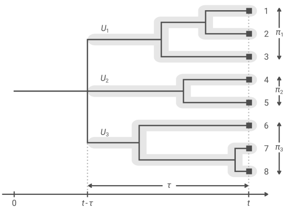
Figure 1: Illustration of a planar ultrametric matrix $U\in\mathbb{U}_{k}$. Here, $k=8$ and the entry $U_{ij}$ corresponds to the coalescence time between the leaves with labels $i$ and $j$, $\tau$ is the distance from the root to the deepest branch point, and $(U_{i})_{i}$ are the distance matrices corresponding to the subtrees that are disconnected by removing the branch point at time $\tau$.

As we shall now see, the moments of the CSBP can be obtained through a planarization argument. Define the space of planar ultrametric matrices with $k$ leaves $\mathbb{U}_{k}$ as the subset of $\mathbb{R}^{k\times k}_{+}$ with the planar ultrametric property which states that, for every $U\in\mathbb{U}_{k}$,

$$\forall i<\ell<j,\quad U_{i,j}=\max(U_{i,\ell},U_{\ell,j}).$$ (21)

Intuitively, one can think of $U\in\mathbb{U}_{k}$ as the distance between the leaves of a plane ultrametric tree with $k$ leaves. See Figure 1.

For every plane ultrametric matrix $U\in\mathbb{U}_{k}$, we define $\tau(U)$ as the depth of the first branch point

$$\forall U\in\mathbb{U}_{k},\quad\tau(U)\coloneqq\max\{U_{i,j}:i,j\in[k]\}.$$

For the next definition, we recall that a composition of $k\in\mathbb{N}\setminus\{0\}$ is an ordered sequence $c=(c_{1},\cdots,c_{p})$ of positive integers such that $\sum_{i=1}^{p}c_{i}=k$. In the following, we denote by $|c|$ the number of elements in the composition. The next definitions are illustrated in Figure 2.

Definition 5.

Let $U\in\mathbb{U}_{k}$. Let $s\in[0,T]$.

1. Let $\pi^{s}(U)$ be the partition of $[k]$ such that $i\sim j$ iff $U_{ij}<s$. Rank the blocks according to their least element and let $B^{s}_{I}(U)\equiv B^{s}_{I}$ the $I^{th}$ block of the partition $\pi^{s}(U)$.

2. Assume that the number of blocks is $p$. Then the vector $c^{s}(U)=(|B^{s}_{1}|,\cdots,|B^{s}_{p}|)$ defines a composition of $[k]$.

3. For every $I\in|c(U)|$, let $U^{s}_{I}(U)\equiv U^{s}_{I}$ denote the ultra-metric plane sub-matrix $(U^{s}_{ij})_{i,j\in B^{s}_{I}}\in\mathbb{U}_{I}$.

4. When $s=\tau$, we will shorten the notation and write $c^{\tau}(U)=c(U)$ and $U^{\tau}_{I}(U)=U_{I}(U)$.

We say that a function $G\colon\mathbb{U}_{k}\to\mathbb{R}$ is of the product form if

$$\forall U\in\mathbb{U}_{k},\quad G(U)=\mathbf{1}_{\{c(U)=c\}}f(\tau(U))\prod_{i=1}^{|c|}F_{i}(U_{i}(U))$$ (22)

for a fixed composition $c$ of $k$, and some continuous bounded functions $f\colon\mathbb{R}_{+}\to\mathbb{R}$ and $F_{i}\colon\mathbb{U}_{c_{i}}\to\mathbb{R}$, $i\leq|c|$. By using the branching property of the reduced process and decomposing ultrametric matrices according to their deepest branching point, we will derive the following result.

Proposition 1.2.

Let $\psi$ be a branching mechanism having some exponential moment. For $t>0$ recall the definition of $\bar{u}_{t}$ as given in (19). For any $k\geq 1$, there exists a unique family of measures $({\mathcal{M}}^{k,t})_{t\geq 0}$ on $\mathbb{U}_{k}$ characterized by the following recursive relation. If $\hat{\cal M}^{k,t}\coloneqq\bar{u}_{t}\mathcal{M}^{k,t}$, then

• For $k=1$ and $t\geq 0$, $\hat{\mathcal{M}}^{1,t}[1]=e^{-bt}$.

• For every $k\geq 2$ and any function $F$ of the product form (22), we have

  $$\hat{\mathcal{M}}^{k,t}[F]=\frac{m_{|c|}}{|c|!}\int_{0}^{t}e^{-b(t-s)}f(s)\prod_{i=1}^{|c|}\hat{\mathcal{M}}^{c_{i},s}[F_{i}]\mathrm{d}s$$ (23)

  where

  $$\forall p\geq 2,\quad m_{p}=(-1)^{p}\psi^{(p)}(0)=\mathbf{1}_{\{p=2\}}d+\int_{0}^{\infty}x^{p}\Lambda(\mathrm{d}x).$$ (24)

For any continuous and bounded function $G\colon\mathbb{R}^{k\times k}_{+}\to\mathbb{R}$,

$$\mathbb{E}\bigg{[}\int_{\mathcal{U}_{t}^{k}}G\big{(}d_{t}(\mathbf{v})\big{)}\,\vartheta_{t}^{\otimes k}(\mathrm{d}\mathbf{v})\bigg{]}=\sum_{P}\mathcal{M}^{k,t}[G\circ P],$$ (25)

where $d(\mathbf{v})=(d(v_{i},v_{j}))_{i,j\leq k}$, the sum is taken over every permutation of $[k]$, and $P$ acts on $\mathbb{U}_{k}$ by permuting the indices of the plane marked matrix.

On the left-hand side of (25), one can identify the moments of the $\psi$-mm space (see Section 1.3). The previous result states that the latter are derived in two successive steps. First, we compute the planar moments recursively from (23). Secondly, we “unplanarize” the moments through the summation on the right-hand side of (25).

1.5 Moments of branching diffusions

1.5.1 Biased spine measure and many-to-few

Consider a general (sub)-critical binary branching diffusions killed at the boundary of a regular domain $\Omega_{\infty}\subseteq\mathbb{R}^{d}$, as introduced in Section 1.2. In this section, and in contrast with Section 1.2, we drop the subscript $\infty$ for a reason that will become apparent in the next section.

Define the random mmm space

$$[{\cal N}_{t},d_{t},\nu_{t}],\ \ \mbox{where $\nu_{t}=\sum_{v\in{\cal N}_{t}}\delta_{v,X_{v}}$}.$$

where for every $u,v\in{\cal N}_{t}$, $d_{t}(u,v)$ denotes the time to the most recent common ancestor of the pair $(u,v)$. The spine process $(\zeta_{t};t\geq 0)$ [26] is the $\mathbb{R}^{d}$-valued process whose generator is given by the Doob $h$-transform of the differential operator ${\cal A}$

$$\frac{{\cal A}(hf)}{h}+wh :=\frac{1}{2}\sum_{i,j}a_{ij}(x)\left(\partial_{x_{i}x_{j}}f(x)+\frac{\partial_{x_{i}}h}{h}\partial_{x_{j}}f(x)+\frac{\partial_{x_{j}}h}{h}\partial_{x_{i}}f(x)\right)$$ (26)

$$\qquad+\sum_{i}b_{i}(x)\partial_{x_{i}}f(x),\quad x\in\Omega,$$

$$f(x) =0,\quad x\in\partial\Omega,$$

where the first equality is a direct consequence of (5). Finally, a direct computation shows that

$$\Pi(dx)=h\tilde{h}(x)dx.$$ (27)

is an invariant probability measure for the system. Let

$$\mathbb{U}_{k}^{*}:=\mathbb{U}_{k}\times E^{k}$$ (28)

be the space of plane marked ultrametric matrices. Recall the definition of test functions of the product form (22) on $\mathbb{U}_{k}$. This definition is extended in a straightforward way to the space of marked plane matrices $\mathbb{U}_{k}^{*}$.

Definition 6 (Biased $k$-spine measure).

Let $t>0$ and $k$ be a positive integer. The biased $k$-spine measure $\mathbf{M}^{k,t}_{x}$ is the unique measure on the space of plane ultrametric matrices $\mathbb{U}^{*}_{k}$ such that

• For $k=1$, for every continuous bounded function $f:\Omega\to\mathbb{R}$

  $$\mathbf{M}_{x}^{1,t}(f)\ =\ e^{-wt}\mathbb{E}_{x}\left[f(\zeta_{t})\right].$$

• For $k\geq 2$, consider test functions of the product form

  $$\forall U^{*}\in\mathbb{U}^{*}_{k},\ G(U^{*})=\mathbf{1}_{\{c(U)=(n,k-n)\}}f(\tau(U))F_{1}(U^{*}_{1})F_{2}(U^{*}_{2})$$ (29)

  where $1\leq n<k$, $F_{1}\colon\mathbb{U}^{*}_{n}\to\mathbb{R}$, $F_{2}\colon\mathbb{U}^{*}_{k-n}\to\mathbb{R}$, and $f\colon[0,t]\to\mathbb{R}$ are continuous and bounded. Then

  $$\mathbf{M}_{x}^{k,t}[G]=\int_{0}^{t}e^{-w(t-u)}f(u)\mathbb{E}_{x}\left[r(\zeta_{t-u})h(\zeta_{t-u})\mathbf{M}_{\zeta_{t-u}}^{n,u}[F_{1}]\mathbf{M}_{\zeta_{t-u}}^{k-n,u}[F_{2}]\right]\mathrm{d}u.$$

  for every function $G$ of the form (29) and $t\geq 0$.

Remark 2.

In [13], and then [26], the authors gave an alternative ”trajectorial” construction of the spine measure. Consider the uniform plane ultrametric tree on $[0,t]$ with $k$ leaves. (In Figure 2, this amounts to drawing the depth $(H_{i})_{i=1}^{k-1}$ to be i.i.d. uniform on $[0,t]$.) Then (1) start a single spine at $x$ at the root, and (2) at every branching point duplicate the spine and run independent copies of the spine process along the branches. Up to a change of measure, $\mathbf{M}^{k,t}_{x}$ describes the joint distribution of the metric structure and the value of the spines at the leaves.

The next result can be seen as the counter-part of Proposition 1.2 for spatial branching processes.

Proposition 1.3 (Many-to-few [26]).

Let $G$ be of the product form (29). Then

$$\mathbb{E}_{x}\bigg{(}\int_{\begin{subarray}{c}(\mathbf{v},\mathbf{x})\in(\mathcal{N}_{t}\times E)^{k}\\ \text{$(v_{i})$ distinct}\end{subarray}}G\big{(}d_{t}({\bf v}),{\bf x})\big{)}(h\nu_{t})^{\otimes k}(d{\bf v},d{\bf x})\bigg{)}=h(x)\sum_{P}{\mathbf{M}}_{x}^{k,t}[G\circ P]$$

where the sum on the right-hand side is taken over every permutation $P$ on $[k]$ and $(h\nu_{t})(dv\otimes dx)\coloneqq h(x)\nu_{t}(dv\otimes dx)$.

Remark 3.

The LHS of the latter identity provides an approximation of a $k^{th}$ moment of the mmm space generated by the branching diffusion at time $t$. Indeed, the system conditioned on survival at large time is typically made of a large number of particles, so that we can can remove the condition $\{(v_{i})\ \ \mbox{distinct}\}$ in the integration. After removing this constraint, the LHS coincides with $k^{th}$ moment of the biased mmm $({\cal N}_{t},d_{t},h\nu_{t})$.

1.6 Main results

1.6.1 Convergence criterium

Let us now consider a critical branching diffusions defined on an infinite domain $\Omega_{\infty}\subseteq\mathbb{R}^{d}$ as in Section 1.2. Recall that $h_{\infty}$ and $\tilde{h}_{\infty}$ are respectively the harmonic functions for ${\cal G}_{\infty}$ and ${\cal G}^{*}_{\infty}$. Recall the definition of $\Omega_{(N,A)}$ given in (7). The heuristics developed in Section 1.2 reveal that if we confine the dynamics in $\Omega_{(N,A)}$, it amounts to removing all the macroscopic jumps of order $A$ (or larger). Thus, in practice, the idea will consist in proving that for any fixed $A$, the size process on $\Omega_{(N,A)}$ converges to a $\psi_{A}$-CSBP where the jump measure in $\psi_{A}$ is obtained by some cutoff of an $\alpha$-stable jump measure.

For every finite domain $\Omega_{(N,A)}$, we assume the existence of $w_{(N,A)},h_{(N,A)},\tilde{h}_{(N,A)}$ as in Section 1.2. Let us now denote by $({\cal N}_{t,(N,A)},d_{t,(N,A)},\nu_{t,(N,A)})$ the metric space induced by the branching diffusions killed on the boundary of $\Omega_{(N,A)}$. $\mathbf{M}_{x,(N,A)}^{k,t}$ denotes the biased $k$-spine measure started from $x$. Define the rescaling operator

$$\forall\left(U,{\bf x}\right)\in{\mathbb{U}}^{*}_{k},\ \ \ S_{N}(U,{\bf x})=(\frac{1}{N}U,{\bf x}).$$ (30)

We introduce the exponent $\gamma$ defined as in (7) and define the rescaled biased $k$-spine measure as

$$\hat{\mathbf{M}}^{k,t}_{x,(N,A)}[F]\ =\ \frac{1}{N^{\gamma(k-1)}}{\mathbf{M}}^{k,Nt}_{x,(N,A)}[F\circ S_{N}].$$ (31)

Theorem 1.

Suppose that the following holds.

1. $\lim_{N\to\infty}h_{(N,A)}(x)=h_{\infty}(x)$ uniformly on compact sets and

   $$\limsup_{N\to\infty}\frac{\sup_{\Omega_{(N,A)}}h_{(N,A)}}{\sup_{\Omega_{(N,A)}}h_{\infty}}=\limsup_{N\to\infty}\sup_{\Omega_{(N,A)}}\frac{h_{(N,A)}}{\bar{c}AN^{\gamma}}<\infty.$$

2. For every $A>0$,

   $$\forall k\geq 1,t\geq 0,\quad\lim_{N\to\infty}\hat{\mathbf{M}}^{k,t}_{x,(N,A)}=\hat{\mathcal{M}}^{k,t}_{(A)}\otimes(h_{\infty}\tilde{h}_{\infty})^{\otimes k},$$ (32)

   where $\hat{\mathcal{M}}^{k,t}_{(A)}$ is defined through the recursive relation of Proposition 1.2 with

   $$\forall k\geq 2,\quad m_{p,(A)}=A^{k-\alpha}\int_{0}^{\infty}x^{p}\Lambda(dx)$$ (33)

   for some measure $\Lambda$ with all moments and $\alpha\in(1,2)$ and $b_{(A)}\in\mathbb{R}$ such that $b_{(A)}\to 0$ as $A\to\infty$.

3. $$\lim_{N\to\infty}\hat{\mathbf{M}}^{k,1}_{x,(N,A)}[1/h_{(N,A)}]\ =\ \hat{\cal M}^{k,1}_{(A)}[1].$$ (34)

Let $(\bar{\cal N}_{t},\bar{d}_{t},\bar{\nu}_{t})=({\cal N}_{tN},\frac{1}{N}d_{tN},\frac{1}{N^{\gamma}}\nu_{tN})$ be the rescaled mmm-space on $\Omega_{\infty}$ starting with a single particle at $x$. Define $\bar{Z}_{t}\ =\ \left<\bar{\nu}_{t},1\right>$. Then there exists $C>0$ such that for $\psi(\theta)=C\theta^{\alpha}$ such that

1. There exists $\eta_{N}\to 0$ such that

   $$\mathbb{P}_{x}(\bar{Z}_{t}>\eta_{N})\sim\frac{\bar{u}_{t}h_{\infty}(x)}{N^{\gamma}},\qquad\text{as $N\to\infty$}.$$

   where $\bar{u}_{t}$ is as defined in (19) for the limiting branching mechanism $\psi$.

2. Conditional on $\{\bar{Z}_{t}>\eta_{N}\}$, we have

   $$(\bar{\cal N}_{t},\bar{d}_{t},\bar{\nu}_{t})\longrightarrow\left(\mathcal{U}_{t},d_{t},\vartheta_{t}\otimes\tilde{h}_{\infty}\right),\qquad\text{as $N\to\infty$}$$

   in distribution for the marked Gromov-weak topology, and where $(\mathcal{U}_{t},d_{t},\vartheta_{t})$ is the $\psi$-mm space as defined in Definition 4.

Remark 4.

1. The first item of this result can be thought of as a weak Kolmogorov estimate for the branching process. It gives the asymptotic of the probability that the process has size of order $N^{\gamma}$.

2. The second part of our results provides two main main informations. First, conditioned on ”weak” survival, the genealogy and the size process of the branching diffusion become indistinguishable from the entrance law of a $\psi$-CSBP. Second, the positions of the particles are i.i.d. and distributed according to the probability density $\tilde{h}^{\infty}$.

3. Let us now comment on the assumptions of the Theorem.

   • Following up on Remark 3, the many-to-one formula (Propostion 1.3) provides an approximate formula for the $h$-biased metric space $(\bar{\cal N}_{t},\bar{d}_{t},h\bar{\nu}_{t})$. Our moment condition ensures that the $h$-biased metric space converges to $\left(\mathcal{U},d_{t},\nu_{t}\otimes\tilde{h}_{\infty}h_{\infty}\right)$.

   • The second part of condition (3) ensures that one can “unbias” the first moment for the constant function $1$. In fact, we will show that this condition is enough to unbias all moments so that the limiting density of the particles is given by $\tilde{h}^{\infty}=\tilde{h}^{\infty}h^{\infty}/h^{\infty}$ as stated in the main conclusion of the Theorem.

   • To get some intuition condition (33), one can consider an $\alpha$-CSBP and the modified process obtained by ignoring all the jumps greater than $A$. A direct computation reveals that the resulting $k$-spine measure satisfy the recursive relation of Proposition 1.2 with $m_{p,(A)}$ satisfying (33) with $\Lambda(dx)$ the Lebesgue measure on $[0,1]$.

1.6.2 Results for the semi-pushed case

For concreteness, we now consider the BBM introduced in Section 1.2.2. In the notation of the previous section, $\Omega=\mathbb{R}_{+}$ and we will choose $\Omega_{(N,A)}=[0,L_{(N,A)}]$ where $L_{(N,A)}\equiv L$ is defined

$$L\equiv L_{(N,A)}=\frac{1}{2\beta}\log(N)+\frac{1}{\mu-\beta}\log(A),$$ (35)

Theorem 2.

Fix $t>0$, and $x\in\mathbb{R}_{+}$. Assume that ($H_{wp}$) holds. Then the conclusions of Theorem 1 hold true.

The previous result shows convergence starting from a single particle. It can be leveraged to prove convergence starting from a large number of particles. In the following, we make a slight abuse of notation and use the same notation as in Theorem 1 but starting with more than one particle.

Theorem 3.

Let ${\bf c}>\frac{1}{\alpha}$ and $z_{0}\geq 0$. Let $b_{\ref{th:cv_mmm}}$ be as in Theorem 2. Suppose that the process starts with an initial configuration satisfying

$$\langle\bar{\nu}_{0},h_{\infty}\rangle\to z_{0},\quad\text{as}\;N\to\infty.$$ (36)

and

$$\mathbb{P}\left(\max_{v\in\bar{\mathcal{N}}_{0}}X_{v}(0)>{\bf c}L_{(N,1)}\right)\to 0,\quad N\to\infty,$$ (37)

Then, for any $0<t_{1}<\dots<t_{p}$ we have

$$\big{(}\bar{Z}_{t_{1}},\dots,\bar{Z}_{t_{p}}\big{)}\to\big{(}\Xi_{t_{1}},\dots,\Xi_{t_{p}}\big{)},\quad N\to\infty,$$

in distribution, where $(\Xi_{t})_{t\geq 0}$ is an $\alpha$-stable CSBP with branching mechanism $\psi(u)=b_{\ref{th:cv_mmm}}u^{\alpha}$ started from $z_{0}$.

1.7 Heuristics and proof strategy for the semi-pushed regime

In view of Theorem 2, a significant fraction of this article will be dedicated to the proof of the following proposition.

Proposition 1.4.

Let ${\bf c}\in(0,1)$ and $A\geq 1$. Uniformly for every $x\in\left[0,{\bf c}L\right]$,

$$\lim_{N\to\infty}\hat{\mathbf{M}}^{k,t}_{x,{(N,A)}}=(\hat{\mathcal{M}}_{(A)}^{k,t}\otimes(h_{\infty}\tilde{h}_{\infty})^{\otimes k}),$$

where where $\hat{\mathcal{M}}^{k,t}_{(A)}$ is defined through the recursive relation of Proposition 1.2 with $m_{p,(A)}$ as in Theorem 1.

We now justify this broad strategy with heuristic computations that will be made rigorous in the rest of the article.

1.7.1 Spectral properties

Recall from Section 1.6.2 that $\lambda_{1,(N,A)}$ and $v_{1,(N,A)}$ are respectively the principal eigenvalue and eigenfunction of the Sturm–Liouville problem (SLP) at $L\equiv L_{(N,A)}$ as in (35). There exists $c_{0}>0$ such that

$$w\equiv w_{(N,A)}\coloneqq\lambda_{1,\infty}-\lambda_{1,(N,A)}=c_{0}e^{-2\beta L}\big{(}1+o_{L}(1)\big{)}.$$

where $\beta=\sqrt{2\lambda_{1,\infty}}$. See Lemma 4.1.

1.7.2 A recursive formula for the planar moments

From now on, we will work with the BBM with an additional killing boundary at $L_{(N,A)}$. We denote by $\mathcal{N}_{t}\equiv\mathcal{N}_{t,(N,A)}$ the set of particles alive at time $t$ in this process. For $v\in\mathcal{N}_{t,(N,A)}$, we still denote by $X_{v}(t)$ its position at time $t$.

Given the cutoff $(N,A)$, we compute the moments of the truncated BBM. In the following $\mathbf{M}_{x}^{k,t}\equiv\mathbf{M}_{x,(N,A)}^{k,t}$ is the corresponding biased $k$-spine measure (as in Definition 6) and $\hat{\mathbf{M}}_{x}^{k,t}\equiv\hat{\mathbf{M}}_{x,(N,A)}^{k,t}$ (see (31)) its rescaled version. According to Definition 6, the building block of the latter quantities is the spine process $(\zeta_{t,(N,A)}\equiv\zeta_{t};t\geq 0)$ on $[0,L_{(N,A)}]$. A direct computation shows that it is the solution to the stochastic differential equation

$$\zeta_{t}=\zeta_{0}+\int_{0}^{t}\frac{v^{\prime}_{1}(\zeta_{s})}{v_{1}(\zeta_{s})}\mathrm{d}s+B_{t}.$$ (38)

In the following, we will denote by $\bar{\zeta}_{t}:=\zeta_{tN}$ the accelerated spine process.

Galton-Watson processes in the domain of attraction of $\alpha$-CSBPs are driven by large branching events. One difficulty of the present model is that we start from a binary branching process, so that the emergence of high-order branching events is not directly visible in the unscaled BBM. (See Proposition 1.3 where the recursion formula for the spinal measures of the BBM only involves binary events.) Thus, it seems a priori unclear how this recursive relation could translate into its $\psi$-CSBP counterpart (33). To overcome this difficulty, we consider functionals of the form

$$\forall U^{*}\in\mathbb{U}^{*}_{k},\quad G^{\varepsilon}(U^{*})=f(\tau(U))\mathbf{1}_{\{c^{\tau-\varepsilon}(U)=c\}}\prod_{i=1}^{|c|}F_{i}(U_{i}^{\tau-\varepsilon})$$ (39)

where all the functions on on the RHS are bounded continuous. By choosing an appropriate $\varepsilon\ll N$ (see below), the branch points occurring during the time interval $[\tau(U)-\varepsilon,\tau(U)]$ are indistinguishable in the limit. This effectively captures the fact that several binary branchings occurring on a short interval cluster into a multifurcation at the limit, leading to multiple mergers of ancestral lineages. Note that for $\varepsilon=0$, the previous definition coincides with the definition of product functionals in (22). In the following, we will write $G^{0}\equiv G$ which is of the classical product form (29). See Figure 2.

Our approach will be based on the following combinatorial formula for the moment evaluated against $G^{\varepsilon}$. In the following, for the $k$-spine measure $\mathbf{M}^{k,t}_{y}$, for $i\leq k$, $X_{i}$ will denote the $i^{th}$ mark. Formally, we recall that $\mathbf{M}^{k,t}_{y}$ is a measure on the space of marked ultrametric plane matrices $\mathbb{U}_{k}\times E^{k}$ where $E$ is the space of marks. ${X_{i}}$ is the projection on the $i^{th}$ mark coordinate. This result is a corollary of the recursive construction of the moments given in Definition 6.

Corollary 1.1.

Let $\bar{\zeta}$ be the spine accelerated by $N$. Let $G^{\varepsilon}$ be of the form $\eqref{eq:Feps}$, for some $\varepsilon>0$. We have

$$\hat{\mathbf{M}}_{x}^{k,t}(G^{\frac{\varepsilon}{N}})=\frac{1}{N^{\gamma(|c|-\alpha)}}\int_{0}^{t}f(u)e^{-Nw(t-u)}\\ \times\mathbb{E}_{x}\left(r(\bar{\zeta}_{t-u})h(\bar{\zeta}_{t-u})\sum_{n=1}^{|c|-1}\mathbf{M}_{\bar{\zeta}_{t-u}}^{j,\varepsilon}\left[\prod_{i=1}^{n}\hat{\mathbf{M}}^{c_{i},u-\frac{\varepsilon}{N}}_{X_{i}}[F_{i}]\right]\mathbf{M}_{\bar{\zeta}_{t-u}}^{|c|-j,\varepsilon}\left[\prod_{i=n+1}^{|c|}\hat{\mathbf{M}}^{c_{j},u-\frac{\varepsilon}{N}}_{X_{i}}[F_{j}]\right]\right)\mathrm{d}u$$ (40)

1.7.3 Step 1.

Let us now argue that the seemingly formula (40) takes a simple form as $N\to\infty$. Let $\Pi$ be the invariant distribution of the spine process. Recall from (27) that

$$\Pi_{(N,A)}(dx)\ =\ h_{(N,A)}\tilde{h}_{(N,A)}(x)dx.$$

is the invariant measure of the spine. The first key observation (Proposition 6.2) is that when $x$ is sufficiently far away from the boundary, $\hat{\mathbf{M}}_{x}^{k,t}(F)$ has no dependence in $x$ and

$$\hat{\mathbf{M}}_{x}^{k,t}(G^{\frac{\varepsilon}{N}})\approx\hat{\mathbf{M}}_{\Pi}^{k,t}(G^{\frac{\varepsilon}{N}})\approx\hat{\mathbf{M}}_{\Pi}^{k,t}(G).$$

provided that $\varepsilon_{N}\to\infty$ and $\varepsilon_{N}/N\to 0$. To get a sense of why this is true, recall from Corollary 1.1 that the only dependence in $x$ in our recursive formula is in the starting position. Since the spine is accelerated by $N$, the term $\bar{\zeta}_{t-u}$ can be replaced by a copy distributed as the invariant measure $\Pi_{(N,A)}$, regardless of the initial position $x$. Under such a substitution, the recursive relation becomes independent in $x$.

Now, consider terms of the form

$$\mathbf{M}_{y}^{j,\varepsilon}\left[\prod_{i=1}^{j}\hat{\mathbf{M}}^{c_{i},u-\frac{\varepsilon}{N}}_{X_{i}}[F_{i}]\right]$$

in (40). For the BBM on $\mathbb{R}_{+}$, we show that if we choose

$$\varepsilon\equiv\varepsilon_{(N,A)}=aL\propto\log N,\qquad a>\frac{2}{\mu-\beta},$$ (41)

then regardless of the starting point $y$ of the $j$-spine, the marks $X_{i}$’s are typically far away from the boundary so that the previous approximation applies, and

$$\forall y\in[0,L],\ \ \mathbf{M}_{y}^{j,\varepsilon}\left[\prod_{i=1}^{j}\hat{\mathbf{M}}^{c_{i},u-\frac{\varepsilon}{N}}_{X_{i}}[F_{i}]\right]\ \approx\ \mathbf{M}_{y}^{j,\varepsilon}[1]\prod_{i=1}^{j}\hat{\mathbf{M}}^{c_{i},u}_{\Pi}[F_{i}]$$

Finally, recall that $\bar{\zeta}$ is the spine accelerated by $N$. As a consequence, the term $\bar{\zeta}_{t-u}$ in (40) is asymptotically distributed as the invariant measure $\Pi$. Let $Y$ be a r.v. with law $\Pi$ and

$$\hat{m}_{|c|}\equiv\hat{m}_{|c|,(N,A)}\coloneqq\frac{|c|!}{N^{\gamma(|c|-\alpha)}}\mathbb{E}_{\Pi}\left(r(Y)h(Y)\sum_{j=1}^{|c|-1}{\mathbf{M}}_{Y}^{j,\varepsilon}[1]{\mathbf{M}}_{Y}^{|c|-j,\varepsilon}[1]\right),$$ (42)

where the expected value is taken w.r.t $y$. Putting the previous estimates together, we get that (Proposition 6.3)

$$\hat{\mathbf{M}}^{k,t}_{\Pi}[G^{0}]=\hat{\mathbf{M}}^{k,t}_{\Pi}[G]\approx\frac{\hat{m}_{|c|,(N,A)}}{|c|!}\int_{0}^{t}f(u)e^{-Nw(t-u)}\prod_{i=1}^{|c|}\hat{\mathbf{M}}_{\Pi}^{c_{i},u}[F_{i}]\mathrm{d}s.$$ (43)

The latter relation mimics the recursive relation for CSBPs as written in Proposition 1.2.

1.7.4 Step 2. The reversed process

According to the recursion formula for the moments of a CSBP, see (23), we now need to identify $\tilde{m}_{k}$, defined in (42), to be the $k$-th moment of a certain jump measure. The key observation is that the invariant distribution of the spine is given by

$$\Pi_{(N,A)}(dx)\ =\ h_{(N,A)}\tilde{h}_{(N,A)}(x)dx.$$

As a consequence, the integral in (42) involves integrating $h^{2}_{(N,A)}\tilde{h}_{(N,A)}$. From (14), there exists $c$ such that for every $x>1$

$$h_{\infty}^{2}\tilde{h}_{\infty}(x)=e^{(\mu-3\beta)x}.$$

In the semi-pushed regime ($H_{wp}$) we have $\mu-3\beta>0$ so that the integration is concentrated at the killing boundary $L$. This reflects that branching points in the BBM are typically typically close to the boundary $L$. See Fig. 2.

Figure 2: Left panel. A plane ultrametric matrix in $\mathbb{U}_{k}$ can be encoded by a plane ultrametric tree. The values $H_{i}$ are interpreted as the depth of the $i^{th}$ branching point and for $i<j$, $U_{ij}=\max{\{H_{i},\cdots,H_{j-1}\}}$ is the distance between the leaves $i$ and $j$. The depth of the tree is given $\tau=\max\{H_{1},\cdots,H_{k-1}\}$. In this figure, the subtrees at depth $\tau-\varepsilon$ partition the leaves are partioned into $5$ blocks. Further, $c^{\tau-\varepsilon}=\{1\}\{2,3\}\{4,5,6\}\{7,8\}\{9\}$. Right panel. Recall the trajectorial interpretation of the spine measure outlined in Remark 2 where branching spine processes are diffusing along the branches of the tree. In (42), most of the mass in the integration is concentrated close to the $L$-boundary which indicates that the first branching point occurs close to the boundary. In the gray time window (depth in $[\tau-\varepsilon,\varepsilon]$), 4 branch points accumulate into a single $4$-furcation at the limit.

When estimating the term ${\mathbf{M}}_{Y}^{j,\varepsilon}[1]$ in (42), it then becomes natural to look at the process from $L$. Reversing the spatial axis, this is a BBM on $[0,L]$ with positive drift $\mu$ and branching rate $r(L-x)$. Since $r(L-x)=\frac{1}{2}$ for $x<L-1$, we will approximate this process by a BBM with a single killing boundary at $0$ and constant branching rate $1/2$. We will call this approximation the the reversed process. The unique boundary of the reversed process is at $0$ and corresponds to the right boundary at $L$ in the original process. The reversed will be a good approximation of the original one until time of order $aL$, where $a<1/\beta$, which will ensure that no particles in the original process enter the interval $[0,1]$ with high probability. Combining this constraint with (41), this leads us to choose

$$\varepsilon=\frac{1-\delta_{1}}{\beta}L=\frac{2(1+\delta_{2})}{\mu-\beta}L$$ (44)

for some $\delta_{1},\delta_{2}>0$.

We now denote by $\overleftarrow{\mathcal{N}_{t}}$ the particles alive at time $t$ in the reversed process, and by $\overleftarrow{X_{v}}(t)$ the position of particle $v\in\overleftarrow{\mathcal{N}_{t}}$ at time $t$. Define

$$\forall z\geq 0,\quad\overleftarrow{v_{1}}(z)=2e^{\beta}\sinh(\beta z),\quad\overleftarrow{\tilde{h}}\!(z)=c_{\infty}\overleftarrow{v_{1}}(z)e^{\mu z},\quad\overleftarrow{h}\!(z)=\frac{1}{c_{\infty}||v_{1,\infty}||_{2}}\overleftarrow{v_{1}}(z)e^{-\mu z},\quad\overleftarrow{\Pi}(z)=\overleftarrow{v_{1}}(z)^{2}.$$ (45)

All these quantities play an analogous role as for the forward process, e.g, $\overleftarrow{\tilde{h}}$ can be interpreted as an invariant measure for the reversed process. Consider the biased $k$-spine measure $\overleftarrow{\mathbf{M}}_{z}^{k,t}$ starting from $z$ defined as in Definition 6 with respect to the reversed process. Changing the variable $x\rightarrow L-x$ in (42) reveals that (Proposition 6.4)

$$\hat{m}_{k,(N,A)}\approx\hat{m}_{k,(\infty,A)}:=\frac{k!}{2||v_{1,\infty}||_{2}}A^{k-\alpha}\int_{0}^{L}\left(\sum_{i=1}^{k-1}\overleftarrow{\mathbf{M}}_{z}^{i,\infty}[1]\overleftarrow{\mathbf{M}}_{z}^{k-i,\infty}[1]\right)\overleftarrow{\Pi}(z)\overleftarrow{h}(z)\mathrm{d}z.$$ (46)

1.7.5 Step 3. Identifying the jump measure.

Our last task is to identify the r.h.s. of (46) to the moments of some measure. This measure will be connected to the distribution of the limit $\overleftarrow{W}_{\infty}$ to the additive Martingale

$$\overleftarrow{W_{t}}\coloneqq\sum_{v\in\overleftarrow{\mathcal{N}_{t}}}\overleftarrow{h}(\overleftarrow{X_{v}}(t)).$$

We will show (Proposition 5.1) that

$$\hat{m}_{k}\approx\frac{2\beta}{||v_{1,\infty}||_{2}}\int_{0}^{\infty}x^{k}\Lambda_{\overleftarrow{W}_{\infty}}(\mathrm{d}x).$$

where the measure $\Lambda_{\overleftarrow{W}_{\infty}}$ is obtained as

$$\Lambda_{\overleftarrow{W}_{\infty}}=\lim_{z\to\infty}\overleftarrow{\tilde{h}}(z){\mathscr{L}_{z}(\overleftarrow{W}_{\infty})}\ \ \mbox{in the vague topology},$$

where $\mathscr{L}_{z}(\overleftarrow{W}_{\infty})$ is the distribution of $\overleftarrow{W}_{\infty}$ when the reversed process started from a single particle at $z$. This result has a natural interpretation. $\overleftarrow{\tilde{h}}$ is the distribution of the particles seen from the boundary $L$. The measure $\Lambda$ is then obtained by picking a particle from the “bulk” according to $\overleftarrow{\tilde{h}}$ and then consider a random number of relaxed particles whose rescaled number is given by the value of the additive martingale $\overleftarrow{W}_{\infty}$.

1.7.6 Completing the proof

Combining the previous three steps, there exists a measure $\Lambda$ such that for $k\geq 2$,

$$\hat{\mathbf{M}}^{k,t}_{\Pi}[G]\approx\frac{A^{k-\alpha}}{|c|!}\left(\int_{0}^{\infty}x^{|c|}\Lambda(\mathrm{d}x)\right)\int_{0}^{t}f(u)e^{-\frac{c_{0}}{A^{\alpha-1}}(t-u)}\prod_{i=1}^{|c|}\hat{\mathbf{M}}^{c_{i},u}_{\Pi}[F_{i}]\mathrm{d}s.$$

We see that the limiting moments of the BBM with a cutoff follow the same recursion as $\hat{\mathcal{M}}^{k,t}_{(A)}$ which is defined through the recursive relation of Proposition 1.2 with

$$\forall k\geq 2,\quad m_{p,(A)}:=A^{k-\alpha}\int_{0}^{\infty}x^{p}\Lambda(dx),\ \ \ \mbox{where $\Lambda:=2\beta\Lambda_{\overleftarrow{W}_{\infty}}$}$$ (47)

for some measure $\Lambda$ with all moments and $b_{(A)}=\frac{c_{0}}{A^{\alpha-1}}\to 0$ as $A\to\infty$. In order to prove Proposition 1.4, it remains to compute the first moment $k=1$. This boils down to the the convergence of the spine process $(\bar{\zeta}_{t})_{t\geq 0}$ to its equilibrium measure $\Pi$.

2 The metric and sampling structure of CSBPs

In this section, we consider general reduced processes, defined as time-inhomogeneous branching processes without death. We show how to construct a random metric measure space out of a reduced process, which encodes the genealogical structure of the boundary of its tree structure. Then, we provide recursive expressions for the moments of this metric measure space and prove some stability results for this class of metric measure spaces. Finally, we apply these results to the reduced processes of Lévy trees introduced by [8], and prove the results stated in the Introduction.

2.1 Reduced processes

Definition of the process.

Consider a collection $(r_{i,\tau})_{i\geq 2,\tau>0}$ of rates, and a fixed time horizon $t>0$. Throughout this section, we will use $s$ for a time variable going in the natural direction of time, and $\tau=t-s$ for the time remaining until the horizon $t$, which is interpreted as the distance to the leaves. We construct a branching particle system where a particle at time $t-\tau$ branches into $i$ daughter particles at rate $r_{i,\tau}$. It will be convenient to use the notation

$$\forall\tau>0,\qquad r_{\tau}=\sum_{i\geq 2}r_{i,\tau},\qquad K_{\tau}\sim\Big{(}\frac{r_{i,\tau}}{r_{\tau}}\Big{)}_{i\geq 2},\qquad m_{\tau}=\sum_{i\geq 2}(i-1)r_{i,\tau}.$$

where $r_{\tau}$ is the total branching rate, $K_{\tau}$ has the law of the number of offspring after a branching event at time $t-\tau$, and $m_{\tau}=\mathbb{E}[K_{\tau}]-1$ is the expected number of new offspring at such an event. We assume that

$$\forall\tau>0,\quad\int_{\tau}^{t}m_{x}\mathrm{d}x<\infty,$$

which will prevent the population from exploding before time $t$.

We construct the branching process as a random tree $\mathcal{T}$, which we encode as a subset of the Ulam–Harris labels

$$\mathcal{V}\coloneqq\{\varnothing\}\cup\bigcup_{n=1}^{\infty}\mathbb{N}^{n}.$$

This tree is further endowed with (continuous) edge lengths, which we represent as a collection of birth times $(\sigma_{u})_{u\in\mathcal{T}}$ and life lengths $(\omega_{u})_{u\in\mathcal{T}}$. The tree $\mathcal{T}$ is constructed iteratively as follows

• we have $\varnothing\in\mathcal{T}$, $\sigma_{\varnothing}=0$, and $(\omega_{\varnothing},K_{\varnothing})$ are distributed as

  $$\mathbb{P}(\omega_{\varnothing}\geq s)=e^{-\int_{0}^{s}r_{t-x}\mathrm{d}x},\quad K_{\varnothing}\sim K_{t-\omega_{\varnothing}};$$

• if $v\in\mathcal{T}$ and $i\leq K_{v}$, $vi\in\mathcal{T}$; define $\sigma_{vi}=\sigma_{v}+\omega_{v}$ and let $(\omega_{vi},K_{vi})$ be distributed as

  $$\mathbb{P}(\omega_{vi}\geq s)=\exp\Big{(}-\int_{\sigma_{vi}}^{\sigma_{vi}+s}r_{t-x}\mathrm{d}x\Big{)},\quad K_{vi}\sim K_{T-\sigma_{vi}-\omega_{vi}}.$$

Let us further denote by

$$\forall s<t,\quad\mathcal{N}_{s,t}\coloneqq\{v\in\mathcal{T}:s\in[\sigma_{v},\sigma_{v}+\omega_{v})\}$$

the set of individuals alive at time $t$, and by

$$\forall s<t,\quad Z_{s,t}\coloneqq\operatorname{Card}\mathcal{N}_{s,t}$$

the size of the population at time $s$.

Reduced processes as random metric measure spaces.

We are interested in the case when $Z_{s,t}\to\infty$ as $s\to t$, which typically arises in the study of genealogies of CSBPs. In that case, the genealogy of the population at time $t$ is a continuous object which we encode as a random metric measure space $(\mathcal{U}_{t},d_{t},\vartheta_{t})$. We carry out the construction of this object carefully in this section, by defining a (discrete) metric measure space representing the genealogy of the reduced process at time $t<T$, and taking a limit in the Gromov-weak topology as $t\to T$.

For $s<t$ and $v,w\in\mathcal{N}_{s,t}$, define the genealogical distance at time $s$ between $v$ and $w$ as

$$\forall v,w\in\mathcal{N}_{s,t},\quad d_{s,t}(v,w)=s-(\sigma_{v\wedge w}+\omega_{v\wedge w})$$

The distance $d_{s,t}(v,w)$ is simply the coalescence time between $v$ and $w$. The pair $(\mathcal{N}_{s,t},d_{s,t})$ can be seen as a random (ultra-)metric space. We endow it with an adequate measure that captures the contribution of each individual to the asymptotic growth of the population. This relies on the fact that $(W_{s,t})_{s<t}$ defined as

$$\forall s<t,\quad W_{s,t}\coloneqq e^{-\int_{0}^{s}m_{t-x}\mathrm{d}x}Z_{s,t}$$

is a non-negative martingale. Its limit, $W_{t}\coloneqq\lim_{s\to t}W_{s,t}$, corresponds to the asymptotic total size of the population. For each $v\in\mathcal{N}_{s,t}$, by the Markov and branching property, the processes

$$\forall x\in[0,t-s),\quad Z^{v}_{x,t-s}\coloneqq\operatorname{Card}\{w\in\mathcal{N}_{s+x,t}:w\succeq v\}$$

are independent for different $v$ and all distributed as $(Z_{x,t-s})_{x<t-s}$. The process simply $Z^{v}_{x,t-s}$ counts the number of descendants of $v$ at time $s+x$. We can define the martingale limit

$$\forall v\in\mathcal{N}_{s,t},\quad W^{v}_{t-s}\coloneqq\lim_{x\to t-s}e^{-\int_{0}^{s+x}m_{t-y}\mathrm{d}y}Z^{v}_{x,t-s}\overset{\mathrm{(d)}}{=}e^{-\int_{0}^{s}m_{t-y}\mathrm{d}y}W_{t-s}.$$

Note that these random variables fulfill that

$$\begin{split}\sum_{v\in\mathcal{N}_{s}}W^{v}_{t-s}&=\lim_{x\to t-s}e^{-\int_{0}^{t-(s+x)}m_{t-y}\mathrm{d}y}\sum_{v\in\mathcal{N}_{s}}Z^{v}_{x,t-s}\\ &=\lim_{x\to t-s}e^{-\int_{0}^{t-(s+x)}m_{t-y}\mathrm{d}y}Z_{s+x,t}=W_{t}.\end{split}$$ (48)

Let us define a measure $\vartheta_{s,t}$ on $\mathcal{N}_{s,t}$ as

$$\vartheta_{s,t}=\sum_{v\in\mathcal{N}_{s,t}}W^{v}_{t-s}\delta_{v}.$$

Then $(\mathcal{N}_{s,t},d_{s,t},\vartheta_{s,t})$ is an ultrametric measure space representing the population at time $s$. We will define the genealogy of the reduced process as the Gromov-weak limit as $s\to t$ of the latter metric measure space. In the next proposition, we make use of Gromov’s box metric $\underline{\Box}_{1}$, defined for instance in [19]. It is a distance between metric measure spaces that induces the Gromov-weak topology, and is equivalent to the more standard Gromov–Prohorov distance [22].

Proposition 2.1.

There exists a random ultrametric measure space $(\mathcal{U}_{t},d_{t},\vartheta_{t}^{\prime})$ such that

$$\lim_{s\to t}(\mathcal{N}_{s,t},d_{s,t},\vartheta_{s,t})=(\mathcal{U}_{t},d_{t},\vartheta_{t}^{\prime})$$

almost surely in the Gromov-weak topology. Moreover the following bound holds almost surely

$$\underline{\Box}_{1}\big{(}(\mathcal{N}_{s,t},d_{s,t},\vartheta_{s,t}),(\mathcal{U}_{t},d_{t},\vartheta_{t}^{\prime})\big{)}\leq t-s.$$ (49)

Proof.

We will show that the sequence is almost surely Cauchy for Gromov’s $\underline{\Box}_{1}$ metric, which is a complete metric generating the Gromov-weak topology. We make use of the formulation of this metric using relations given in [19, Definition 3.2].

Fix $s<s^{\prime}$. We construct a relation $R\subseteq\mathcal{N}_{s,t}\times\mathcal{N}_{s^{\prime},t}$ as

$$(v,v^{\prime})\in R\iff v\preceq v^{\prime}$$

as well as a measure $\pi$ on $\mathcal{N}_{s,t}\times\mathcal{N}_{s^{\prime},t}$ as

$$\pi(\{(v,v^{\prime})\})=\mathbf{1}_{\{v\preceq v^{\prime}\}}W^{v^{\prime}}_{t}.$$

Quite clearly, the projection of $\pi$ on $\mathcal{N}_{s,t}$ (resp. $\mathcal{N}_{s^{\prime},t}$) coincides with $\nu_{s,t}$ (resp. $\nu_{s^{\prime},t}$) and $\pi(R)=W_{t}$. This checks condition (3.3) of [19, Definition 3.2] for any $\varepsilon>0$.

Let $(v,v^{\prime}),(w,w^{\prime})\in R$, we show that

$$|d_{s,t}(v,w)-d_{s^{\prime},t}(v^{\prime},w^{\prime})|\leq s^{\prime}-s.$$

If $v=w$, then $d_{s,t}(v,w)=0$ and $v^{\prime}$ and $w^{\prime}$ find a common ancestor before time $t$, thus

$$d_{s^{\prime},t}(v^{\prime},w^{\prime})\leq s^{\prime}-s.$$

Conversely if $v\neq w$, then $v\wedge w=v^{\prime}\wedge w^{\prime}$ and thus

$$d_{s^{\prime},t}(v^{\prime},w^{\prime})-d_{s,t}(v,w)=s^{\prime}-s$$

hence the result. This shows that condition (3.4) of [19, Definition 3.2] is fulfilled for $\varepsilon=s^{\prime}-s$ and therefore that

$$\underline{\Box}_{1}(\mathcal{N}_{s,t},\mathcal{N}_{s^{\prime},t})\leq s^{\prime}-s\to 0.$$

The bound (49) is obtained by letting $s^{\prime}\to t$ in the previous inequality. ∎

Remark 5.

A direct construction that does not involve a limit could be obtained by considering the boundary of $\mathcal{T}$ and endowing it with a measure using Caratheodory’s extension theorem, as is for instance carried out in [7, Section 2.1]. This construction would, moreover, endow the limit tree with a planar ordering. However, it is not straightforward to compute the moments directly on the continuous object, and our construction will allow us to carry out the computation on the discrete trees and to take a limit.

2.2 Moments of reduced processes

Decomposing ultrametric trees.

Recall the notation $\mathbb{U}_{k}$ for the set of planar ultrametric matrices of Section 1.4.2, and for $U\in\mathbb{U}_{k}$, the notation $\tau(U)$, $c(U)$ and $(U_{i}(U))_{i})$ from Definition 5. The moments of reduced processes will take an elegant recursive form for functionals $G\colon\mathbb{U}_{k}\to\mathbb{R}$ of the product form introduced in (22) that we recall here,

$$\forall U\in\mathbb{U}_{k},\quad G(U)=\mathbf{1}_{\{c(U)=c\}}f(\tau(U))\prod_{i=1}^{|c|}F_{i}(U_{i}(U)),$$

where $c$ is a composition of $k$, and $f\colon R_{+}\to\mathbb{R}$ and $F_{i}\colon\mathbb{U}_{c_{i}}\to\mathbb{R}$, $i\leq|c|$ are continuous bounded functions.

Before computing the moments, we need a technical result that deals with the fact that branch points might accumulate, and as a consequence the map $U\mapsto(\tau(U),c(U),(U_{i}(U))_{i})$ is not continuous at $U$ if $|c(U)|\geq 2$. First, notice that the inverse map $(\tau(U),c(U),(U_{i}(U))_{i})\mapsto U$ that concatenates the subtrees is continuous. Recall the notation $\pi(U)$ of Section 1.4.2 for the partition of the leaves of $U$ in consecutive subtrees. We have that

$$\forall m,n\leq k,\quad U_{m,n}=\begin{dcases}\tau(U)&\text{if $m\not\sim_{\pi(U)}n$}\\ (U_{i})_{m-\ell_{i},n-\ell_{i}}&\text{if $m,n\in\pi_{i}(U)$}\end{dcases}$$ (50)

where we have defined $\ell_{i}=\min\pi_{i}(U)-1$.

Lemma 2.1.

Let $(U^{p},p\geq 1)$ be a sequence of random ultrametric planar trees with $k$ leaves. Suppose that

$$\big{(}\tau(U^{p}),c(U^{p}),(U^{p}_{i})_{i\leq|c(U^{p})|}\big{)}\to\big{(}\tau,c,(U^{\prime}_{i})_{i\leq|c|}\big{)}$$ (51)

in distribution as $p\to\infty$. Then, there exists a limit random element $U\in\mathbb{U}_{k}$ such that $U^{p}\to U$ in distribution as $p\to\infty$. Furthermore, if $\tau(U^{\prime}_{i})>0$ almost surely for all $i\leq|c|$, then

$$\big{(}\tau(U),c(U),(U_{i})_{i\leq|c|}\big{)}\overset{\mathrm{(d)}}{=}\big{(}\tau,c,(U^{\prime}_{i})_{i\leq|c|}\big{)}$$

Proof.

Let $U$ be the random plane ultrametric space constructed as in (50), using the limit variables $(\tau,c,(U^{\prime}_{i})_{i\leq|c|})$. By the explicit expression (50), we see that (51) ensures that $U^{p}\to U$ as $p\to\infty$.

The second part of the result is not an immediate consequence of the convergence $U^{p}\to U$ because the application $U\mapsto(\tau(U),c(U),(U_{i})_{i})$ is not continuous due to possible accumulation of branch points. Using Skorohod’s representation theorem, let us assume that the convergence occurs almost surely. Let $\pi(U^{p})$ be the partition of $\{1,\dots,k\}$ defined in Definition 5 and recall that $(\pi_{i}(U^{p}))_{i\leq|c(U^{p})|}$ denote its blocks. For $m,n\in\pi_{i}(U^{p})$,

$$U^{p}_{m,n}\leq T-\tau(U^{p})-\tau(U^{p}_{i}).$$

Therefore, since $\tau(U^{\prime}_{i})>0$ almost surely,

$$U_{m,n}=\lim_{p\to\infty}U^{p}_{m,n}\leq T-\tau-\tau(U^{\prime}_{i})<T-\tau.$$

Thus, $c(U)=\lim_{p\to\infty}c(U^{p})=c$. Since $(U^{p}_{i})_{i\leq|c(U^{p})|}$ is the submatrix of $U^{p}$ with indices in $\pi_{i}(U^{p})$ and $\pi(U^{p})$ converges to $\pi(U)$, we have that

$$U_{i}=\lim_{p\to\infty}U^{p}_{i}=U^{\prime}_{i},$$

hence the result. ∎

Computing the moments.

The aim of this section is to compute the Gromov-weak moments of the tree $(\mathcal{U}_{t},d_{t},\vartheta_{t}^{\prime})$. We start by deriving a many-to-few formula, which will allow us to compute the moments of the discrete tree $(\mathcal{N}_{s,t},d_{s,t},\vartheta_{s,t})$. Define a measure $\mathcal{M}^{k,s,t}$ on $\mathbb{U}^{k}$ such that, for any continuous bounded $G\colon\mathbb{U}_{k}\to\mathbb{R}$, we have

$$\mathcal{M}^{k,s,t}[G]=\mathbb{E}\Big{[}\sum_{\begin{subarray}{c}v_{1},\dots,v_{k}\in\mathcal{N}_{s,t}\\ v_{1}<\dots<v_{k}\end{subarray}}G\big{(}U_{s}(\mathbf{v})\big{)}\Big{]}.$$ (52)

where $U_{s}(\mathbf{v})=(d_{s}(v_{i},v_{j}))_{i,j\leq k}$ is the planar ultrametric matrix encoding the pairwise distances of $\mathbf{v}=(v_{1},\dots,v_{k})$. This corresponds to a planar version of the moments of the mm-space $(\mathcal{N}_{s,t},d_{s,t},\vartheta_{s,t})$.

Proposition 2.2 (Many-to-few).

Let $G$ be a functional of the form (22). Then,

$$\mathcal{M}^{k,s,t}[G]=\frac{1}{|c|!}\int_{0}^{s}r_{t-x}\mathbb{E}[K_{t-x}^{(|c|)}]f(s-x)e^{\int_{0}^{x}m_{t-y}\mathrm{d}y}\prod_{i=1}^{|c|}\mathcal{M}^{c_{i},s-x,t-x}[F_{i}]\mathrm{d}x.$$

Proof.

Fix a composition $c$ of $k$ with $|c|=d$ blocks, and let us write $\pi$ for the partition of $\{1,\dots,k\}$ made of blocks of consecutive integers with length $(c_{1},\dots,c_{d})$. If $w=v_{1}\wedge\dots\wedge v_{k}$, in order to have $c(U_{t}(\mathbf{v}))=c$, there need to exist $|c|=d$ labels $p_{1}<\dots<p_{d}\leq K_{w}$ such that, for each $i\leq d$, $wp_{i}$ is the offspring of $w$ from which each $j\in\pi_{i}$ is descended, that is, $wp_{i}\preceq v_{j}$, $j\in\pi_{i}$. This allows us to re-write the sum in the right-hand side of (52) as

$$\sum_{\begin{subarray}{c}(v_{j})\in\mathcal{N}_{s,t}\\ v_{1}<\dots<v_{k}\end{subarray}}f(\tau(U_{s}(\mathbf{v})))\mathbf{1}_{\{c(U_{s}(\mathbf{v}))=c\}}\prod_{i=1}^{|c|}F_{i}(U_{s,i}(\mathbf{v}))$$

$$=\sum_{w}\mathbf{1}_{\{\sigma_{w}+\omega_{w}<s\}}f(s-\sigma_{w}-\omega_{w})\sum_{\begin{subarray}{c}p_{1},\dots,p_{|c|}=1\\ p_{1}<\dots<p_{|c|}\end{subarray}}^{K_{w}}\prod_{i=1}^{|c|}\sum_{\begin{subarray}{c}v^{i}_{1}<\dots<v^{i}_{c_{i}}\in\mathcal{N}_{s,t}\\ wp_{i}\preceq v^{i}_{j}\end{subarray}}F_{i}(U_{s}(\mathbf{v}^{i})),$$

where we used the notation $\mathbf{v}^{i}=(v^{i}_{j})_{j}$ and $U_{s,i}(\mathbf{v})=U_{i}(U_{s}(\mathbf{v}))$. Now, applying the strong Markov and the branching property yields that

$$\mathbb{E}\Big{[}\sum_{\begin{subarray}{c}(v_{j})\in\mathcal{N}_{s,t}\\ v_{1}<\dots<v_{k}\end{subarray}} f(\tau(U_{s}))\mathbf{1}_{\{c(U_{s})=c\}}\prod_{i=1}^{|c|}F_{i}(U_{i})\Big{]}$$

$$=\mathbb{E}\Big{[}\sum_{w}\mathbf{1}_{\{\sigma_{w}+\omega_{w}<t\}}f(s-\sigma_{w}-\omega_{w})\frac{K_{w}^{(|c|)}}{|c|!}\prod_{i=1}^{|c|}\mathcal{M}^{c_{i},s-\sigma_{w}+\omega_{w},t-\sigma_{w}+\omega_{w}}[F_{i}]\Big{]}$$

$$=\int_{0}^{s}\frac{1}{|c|!}e^{\int_{0}^{t-x}m_{y}\mathrm{d}y}r_{t-x}\mathbb{E}[K_{t-x}^{(|c|)}]f(s-x)\prod_{i=1}^{|c|}\mathcal{M}^{c_{i},s-x,t-x}[F_{i}]\mathrm{d}x$$

where in the last line we have used that $K_{w}\sim K_{\sigma_{w}+\omega_{w}}$, and that the branching times $(\sigma_{w}+\omega_{w})_{w\in\mathcal{V}}$ form a point process with intensity $r_{t-x}e^{\int_{0}^{t-x}m_{y}\mathrm{d}y}\mathrm{d}x$. ∎

Corollary 2.1 (Moments of reduced processes).

Suppose that, for any $t>0$, we have

$$\forall k\geq 2,\quad\sup_{0<s\leq t}r_{s}\mathbb{E}[K_{s}^{(k)}]e^{-(k-1)\int_{0}^{t-s}m_{t-x}\mathrm{d}x}<\infty,\qquad\int_{0}^{t}m_{s}\mathrm{d}s=\infty.$$ (53)

Define a family of measure $(\mathcal{M}^{k,t})_{t\geq 0}$ on $\mathbb{U}^{k}$ inductively on $k$ as follows. For $k=1$, $\mathcal{M}^{1,t}[1]=1$. For $k\geq 2$ and any functional $G$ of the product form (22),

$$\mathcal{M}^{k,T}[G]=\frac{1}{|c|!}\int_{0}^{t}r_{s}\mathbb{E}[K^{(|c|)}_{s}]f(s)e^{-(k-1)\int_{s}^{t}m_{x}\mathrm{d}x}\prod_{i=1}^{|c|}\mathcal{M}^{c_{i},s}[F_{i}]\mathrm{d}s.$$ (54)

Then, the moments of $(\mathcal{U}_{t},d_{t},\vartheta^{\prime}_{t})$ are given by

$$\mathbb{E}\Big{[}\int_{\mathcal{U}_{t}^{k}}G\big{(}d_{t}(\mathbf{v})\big{)}{\vartheta^{\prime}_{t}}^{\otimes k}(\mathrm{d}\mathbf{v})\big{)}\Big{]}=\sum_{P}\mathcal{M}^{k,t}[G\circ P]$$

where $d_{t}(\mathbf{v})=(d_{t}(v_{i},v_{j}))_{i,j\leq k}$ and the sum is taken over all permutations $P$ of $\{1,\dots,k\}$.

Proof.

By applying the many-to-few formula, Proposition 2.2, we see that

$$\mathbb{E}[W^{k}_{s,t}] =e^{-k\int_{0}^{s}m_{t-y}\mathrm{d}y}\mathbb{E}[Z_{s,t}^{k}]$$

$$=e^{-k\int_{0}^{s}m_{t-y}\mathrm{d}y}\sum_{c}\frac{1}{|c|!}\int_{0}^{s}r_{t-x}\mathbb{E}[K^{(c)}_{t-x}]e^{\int_{0}^{x}m_{t-y}\mathrm{d}y}\prod_{i=1}^{|c|}\mathbb{E}[Z_{s-x,t-x}^{c_{i}}]\mathrm{d}x$$

$$=\sum_{c}\frac{1}{|c|!}\int_{0}^{s}r_{t-x}\mathbb{E}[K^{(c)}_{t-x}]e^{-(k-1)\int_{0}^{x}m_{t-y}\mathrm{d}y}\prod_{i=1}^{|c|}\mathbb{E}[W_{s-x,t-x}^{c_{i}}]\mathrm{d}x,$$ (55)

where the sum is over all compositions $c$ of $\{1,\dots,k\}$ except $(1,\dots,1)$. For $k=2$, using that $(W_{s,t})_{s<t}$ is a martingale and (53) yields that,

$$\forall T>0,\quad\sup_{0\leq s<t\leq T}\mathbb{E}[W^{2}_{s,t}]<\infty.$$

This shows that $(W_{s,t})_{s<t}$ is uniformly integrable, and therefore $\mathbb{E}[W_{s,t}]\to\mathbb{E}[W_{t}]=1$, as $s\to t$.

We prove by induction on $k$ that (1) the limit

$$\mathcal{M}^{k,t}\coloneqq\lim_{s\to t}e^{-k\int_{0}^{s}m_{t-y}\mathrm{d}y}\mathcal{M}^{k,s,t}$$ (56)

exists in the sense of weak convergence of measures on $\mathbb{U}_{k}$, (2) that its fulfills (54), (3) that

$$\forall T>0,\quad\sup_{0\leq s<t\leq T}\mathbb{E}[W^{k}_{s,t}]<\infty,$$ (57)

and (4) that $\mathcal{M}^{k,t}(\{U\in\mathbb{U}_{k}:\tau(U)=t\})=0$. For $k=1$, the result follows from the uniform integrability of $(W_{s,t})_{s<t}$. Fix some $k\geq 2$, and let us assume that the claim holds for all $p<k$.

First, by (55) and (53) we have

$$\forall T>0,\quad\sup_{0\leq s<t\leq T}\mathbb{E}[W^{k}_{s,t}]<\infty,$$

and hence (57) holds. For (56) we apply the many-to-few formula, Proposition 2.2, to get that, if $G$ is of the form (22),

$$e^{-k\int_{0}^{s}m_{t-y}\mathrm{d}y} \mathcal{M}^{k,s,t}[G]=e^{-k\int_{0}^{s}m_{t-y}\mathrm{d}y}\frac{1}{|c|!}\int_{0}^{s}r_{t-x}\mathbb{E}[K_{t-x}^{(|c|)}]f(s-x)e^{\int_{0}^{x}m_{t-y}\mathrm{d}y}\prod_{i=1}^{|c|}\mathcal{M}^{c_{i},s-x,t-x}[F_{i}]\mathrm{d}x$$

$$=\frac{1}{|c|!}\int_{0}^{s}r_{t-x}\mathbb{E}[K_{t-x}^{(|c|)}]f(s-x)e^{-(k-1)\int_{0}^{x}m_{t-y}\mathrm{d}y}\prod_{i=1}^{|c|}e^{-\int_{0}^{s-x}m_{t-x-y}\mathrm{d}y}\mathcal{M}^{c_{i},s-x,t-x}[F_{i}]\mathrm{d}x.$$

The dominated convergence theorem, using (56) for the convergence of the integrand and the bound (57), shows that

$$\lim_{s\to t}e^{-k\int_{0}^{s}m_{t-y}\mathrm{d}y}\mathcal{M}^{k,s,t}[F]=\frac{1}{|c|!}\int_{0}^{t}r_{t-x}\mathbb{E}[K^{(|c|)}_{t-x}]f(t-x)e^{-(k-1)\int_{0}^{x}m_{t-y}\mathrm{d}y}\prod_{i=1}^{|c|}\mathcal{M}^{c_{i},t-x}[F_{i}]\mathrm{d}x.$$ (58)

Let $U_{s,t}\in\mathbb{U}_{k}$ be “distributed” as $e^{-k\int_{0}^{s}m_{t-y}\mathrm{d}y}\mathcal{M}^{k,s,t}$. (In an improper sense since it is not a probability measure.) The convergence for product functionals (58) shows that $(\tau(U_{s,t}),c(U_{s,t}),(U_{s,t,i})_{i\leq|c(U_{s,t})|})$ converge “in distribution” as $s\to t$ (again in an improper sense) to some limit $(\tau(U_{t}),c(U_{t}),(U_{i,t})_{i\leq|c(U_{t})|})$ whose law follows the recursion (54). By our induction step, $\tau(U_{t,i})>0$ almost surely, for $i\leq|c(U_{t})|$. Therefore, Lemma 2.1 shows that there exists a limit

$$\mathcal{M}^{k,t}\coloneqq\lim_{s\to t}e^{-k\int_{0}^{s}m_{t-y}\mathrm{d}y}\mathcal{M}^{k,s,t}$$

for the weak topology on measures on $\mathbb{U}_{k}$, and that

$$\lim_{s\to t}e^{-k\int_{0}^{s}m_{t-y}\mathrm{d}y}\mathcal{M}^{k,s,t}[G]=\mathcal{M}^{t,t}[G]$$

holds for $G$ of the form (22), so that the measure fulfills the recursion (54). (Note that this is not guaranteed by weak convergence since product functionals are not continuous.) It is clear from (58) that $\mathcal{M}^{k,t}(\{\tau(U)=0\})=0$ (the “law” of $\tau(U)$ under $\mathcal{M}^{k,t}$ has a density with respect to the Lebesgue measure), which ends the induction.

By definition of $\mathcal{M}^{k,s,t}$, see (52),

$$\mathbb{E}\Big{[}\sum_{\begin{subarray}{c}v_{1},\dots,v_{k}\in\mathcal{N}_{s,t}\\ \text{$(v_{i})$ distinct}\end{subarray}}G(U_{s}(\mathbf{v}))\Big{]}=\sum_{P}\mathcal{M}^{k,s,t}[G\circ P],$$

where the sum is taken over all partitions of $\{1,\dots,k\}$. Therefore, the result is proved in we can show that, for any continuous bounded $G\colon\mathbb{U}_{k}\to\mathbb{R}$,

$$\lim_{s\to t}e^{-k\int_{0}^{s}m_{t-y}\mathrm{d}y}\mathbb{E}\Big{[}\sum_{\begin{subarray}{c}v_{1},\dots,v_{k}\in\mathcal{N}_{s,t}\\ \text{$(v_{i})$ distinct}\end{subarray}}G(U_{s}(\mathbf{v}))\Big{]}=\mathbb{E}\Big{[}\int_{\mathcal{U}_{t}^{k}}G\big{(}d_{t}(\mathbf{v})\big{)}{\vartheta^{\prime}_{t}}^{\otimes k}(\mathrm{d}\mathbf{v})\Big{]}.$$ (59)

Without loss of generality, by Portmanteau’s theorem, we can assume that $G$ is Lipschitz. Let $\Phi$ be the polynomial constructed as in (16) from $\phi=G$. Using the uniform estimate (49) and Lemma A.1, we have that

$$\big{|}\mathbb{E}\left[\Phi(\mathcal{N}_{s,t},d_{s,t},\vartheta_{s,t})\right]-\mathbb{E}\left[\Phi(\mathcal{U}_{t},d_{t},\vartheta^{\prime}_{t})\right]\big{|}=O(|t-s|).$$ (60)

Moreover, by definition of the measures $\vartheta_{s,t}$,

$$\mathbb{E}\big{[}\Phi(\mathcal{N}_{s,t},d_{s,t},\vartheta_{s,t})\big{]} =\mathbb{E}\Big{[}\sum_{(v_{1},\dots,v_{k})\in\mathcal{N}_{s,t}}G(U_{s}(\mathbf{v}))\prod_{i=1}^{k}W^{v_{i}}_{t-s}\Big{]}$$

$$=\mathbb{E}\Big{[}\sum_{(v_{1},\dots,v_{k})\in\mathcal{N}_{s,t}}G(U_{s}(\mathbf{v}))\mathbb{E}\Big{[}\prod_{i=1}^{k}W^{v_{i}}_{t-s}\Big{]}\Big{]}.$$

Recall that $(W^{v}_{t-s})_{v\in\mathcal{N}_{s,t}}$ are i.i.d. and distributed as $e^{-\int_{0}^{s}m_{t-y}\mathrm{d}y}W_{t-s}$. Therefore, (57) shows that, for any $(v_{1},\dots,v_{k})\in\mathcal{N}_{s,t}$,

$$\mathbb{E}\Big{[}\prod_{i=1}^{k}W^{v_{i}}_{t-s}\Big{]}=O\Big{(}e^{-k\int_{0}^{s}m_{t-y}\mathrm{d}y}\Big{)}.$$

Hence, using that $Z^{k}_{s,t}-Z^{(k)}_{s,t}=O(Z^{k-1}_{s,t})$,

$$\mathbb{E}\big{[} \Phi(\mathcal{N}_{s,t},d_{s,t},\vartheta_{s,t})\big{]}$$

$$=\mathbb{E}\Big{[}\sum_{\begin{subarray}{c}(v_{1},\dots,v_{k})\in\mathcal{N}_{s,t}\\ \text{$(v_{i})$ distinct}\end{subarray}}G(U_{s}(\mathbf{v}))\prod_{i=1}^{k}W^{v_{i}}_{t-s}\Big{]}+O\Big{(}e^{-k\int_{0}^{s}m_{t-y}\mathrm{d}y}\mathbb{E}[Z_{s,t}^{k-1}]\Big{)}$$

$$=e^{-k\int_{0}^{s}m_{t-y}\mathrm{d}y}\mathbb{E}\Big{[}\sum_{\begin{subarray}{c}(v_{1},\dots,v_{k})\in\mathcal{N}_{s,t}\\ \text{$(v_{i})$ distinct}\end{subarray}}G(U_{s}(\mathbf{v}))\Big{]}+e^{-\int_{0}^{s}m_{t-y}\mathrm{d}y}O\Big{(}\mathbb{E}[W_{s,t}^{k-1}]\Big{)}.$$

The error term vanishes because of (57) and our second assumption on the rates (53), and we obtain our result by the convergence of the moments (56) and the bound (59). ∎

2.3 Convergence of reduced processes

The moments computations presented so far will enable us to prove convergence of the genealogies with a cutoff. In order to show that the cutoff is a good approximation of the original process, we need a convergence result that does not rely on moments. It will be provided by the following result.

Proposition 2.3.

Let $(\mathcal{U}_{t}^{j},d_{t}^{j},{\vartheta^{\prime}_{t}}^{j})_{j\geq 1}$ be a sequence of ultrametric spaces corresponding to a sequence of reduced processes $(Z^{j}_{s,t};\,s<t)_{j\geq 1}$. Suppose that there exists a reduced process $(Z_{s,t};\,s<t)$ such that:

1. For each $\tau>0$, $((r^{j}_{i,\tau})_{i\geq 2})_{j\geq 1}$ converges in $\ell^{1}$ as $j\to\infty$ to the sequence $(r_{i,\tau})_{i\geq 2}$, and that $(r^{j}_{\tau})_{j\geq 1}$ is bounded uniformly in $\tau$.

2. For each $t>0$, $W^{j}_{t}\to W_{t}$.

Then $(\mathcal{U}_{t}^{j},d_{t}^{j},{\vartheta^{\prime}_{t}}^{j})_{j\geq 1}$ converges in distribution to $(\mathcal{U}_{t},d_{t},\vartheta^{\prime}_{t})$ in the Gromov-weak topology.

Proof.

By the uniform bound in (49), it is sufficient to show that, for all fixed $s<t$, $(\mathcal{N}^{j}_{s,t},d_{s,t}^{j},\vartheta^{j}_{t,T})\to(\mathcal{N}_{s,t},d_{s,t},\vartheta_{s,t})$ as $j\to\infty$.

Fix $s<t$. It is not hard to see that the first point of our assumptions is sufficient to obtain the joint convergence in distribution as $j\to\infty$ of $(\mathcal{N}^{j}_{s,t},(\sigma^{j}_{v},\omega^{j}_{v})_{v:\sigma^{j}_{v}\leq s})$ to $(\mathcal{N}_{s,t},(\sigma_{v},\omega_{v})_{v:\sigma_{v}\leq s})$. Since conditional on $(\mathcal{N}^{j}_{s,t},(\sigma^{j}_{v},\omega^{j}_{v})_{v:\sigma^{j}_{v}\leq s})$ the weights $(W^{j,v}_{t-s})_{v\in\mathcal{N}^{j}_{s,t}}$ are i.i.d. and distributed as a multiple of $W^{j}_{t-s}$, the second point of our assumption actually shows that

$$(\mathcal{N}^{j}_{s,t},(\sigma^{j}_{v},\omega^{j}_{v})_{v:\sigma^{j}_{v}\leq s},(W^{v,j}_{t-s})_{v\in\mathcal{N}^{j}_{s,t}})\to(\mathcal{N}_{s,t},(\sigma_{v},\omega_{v})_{v:\sigma_{v}\leq s},(W^{v}_{t-s})_{v\in\mathcal{N}_{s,t}})$$

jointly in distribution as $j\to\infty$. Up to using Skorohod representation theorem, we can assume that these variables are deterministic. For $j$ large enough, $\mathcal{N}^{j}_{s,t}=\mathcal{N}_{s,t}$, and by the definition of $(\mathcal{N}^{j}_{s,t},d^{j}_{s,t},\vartheta^{j}_{s,t})$,

$$\forall v,w\in\mathcal{N}_{s,t},\quad\lim_{j\to\infty}d^{j}_{s,t}(v,w)=d_{s,t}(v,w),\quad\lim_{j\to\infty}\vartheta_{s,t}^{j}(\{v\})=\vartheta_{s,t}(\{v\}).$$

It is not hard to see that this entails a Gromov-weak convergence of the corresponding metric measure spaces. ∎

2.4 The genealogy of CSBPs

We now apply the results proved for general reduced processes to the special case of the reduced processes giving the genealogy of a CSBP. Recall the notation for CSBPs from Section 1.4, in particular the notation $\bar{u}_{t}$ for the limit of the Laplace exponent under Grey’s condition. Under the same condition, we can define for each $t>0$ a random variable $\bar{\Xi}_{t}$ corresponding to the law of the CSBP “started from $0$” and conditioned on survival. It can be defined through its Laplace transform

$$\forall\theta\geq 0,\quad\bar{u}_{t}\mathbb{E}[1-e^{-\theta\bar{\Xi}_{t}}]=u_{t}(\theta).$$ (61)

We will refer to this random variable as being distributed under the entrance law of the CSBP.

We prove two results in this final section. The first one is the computation of moments for the $\psi$-CSBP, Proposition 1.2. The second one is a stability result for CSBPs, which we will need in our proofs when letting the precision of the cutoff $A$ go to infinity. Let us start with the proof of Proposition 1.2.

Proof of Proposition 1.2.

Let us denote by $G_{t}(\theta)=r_{t}\mathbb{E}[\theta^{K_{t}}]$ the generating function in (20). We obtain the factorial moments of $K_{t}$ by deriving successively $G_{t}$. First, we have that

$$r_{t}=G_{t}(1)=\psi^{\prime}(\bar{u}_{t})-\frac{\psi(\bar{u}_{t})-\psi(0)}{\bar{u}_{t}}$$

and

$$\partial_{\theta}G_{t}(\theta)=\psi^{\prime}(\bar{u}_{t})-\psi^{\prime}((1-\theta)\bar{u}_{t}),$$

so that

$$m_{t}=r_{t}\mathbb{E}[K_{t}-1]=\partial_{\theta}G_{t}(1)-G_{t}(1)=\frac{\psi(\bar{u}_{t})}{\bar{u}_{t}}-\psi^{\prime}(0)=\frac{\psi(\bar{u}_{t})}{\bar{u}_{t}}-b.$$

By taking further derivatives we obtain

$$r_{t}\mathbb{E}[K^{(k)}_{t}]=\partial_{\theta}^{k}G_{t}(1)=(-1)^{k}\bar{u}_{t}^{k-1}\psi^{(k)}(0)=\bar{u}_{t}^{k-1}\Big{(}\mathbf{1}_{\{k=2\}}d+\int_{0}^{\infty}x^{k}\Lambda(\mathrm{d}x)\Big{)}.$$

Moreover,

$$\forall 0<s\leq t,\quad\int_{s}^{t}\frac{\psi(\bar{u}_{x})}{\bar{u}_{x}}\mathrm{d}x=-\int_{s}^{t}\frac{\bar{u}^{\prime}_{x}}{\bar{u}_{x}}\mathrm{d}x=\log\bar{u}_{s}-\log\bar{u}_{t},$$

from which we deduce that

$$\forall s<t,\quad e^{-\int_{0}^{s}m_{t-s^{\prime}}\mathrm{d}s^{\prime}}=\frac{\bar{u}_{t}}{\bar{u}_{t-s}}e^{sb}.$$ (62)

It can be directly checked from this expression using that $\bar{u}_{t}\to\infty$ as $t\to 0$ that the two conditions in (53) are fulfilled. Therefore, Corollary 2.1 ensures that

$$\bar{u}_{t}\mathcal{M}^{k,t}[G] =\begin{multlined}\frac{e^{-kbt}}{\bar{u}_{t}^{k-1}}\frac{1}{|c|!}\int_{0}^{t}f(t-s)r_{t-s}\mathbb{E}[K^{(|c|)}_{t-s}]e^{-(k-1)\int_{0}^{s}m_{t-s^{\prime}}\mathrm{d}s^{\prime}}\\ \times\prod_{i=1}^{|c|}\bar{u}_{t-s}^{c_{i}}e^{c_{i}b(t-s)}\mathcal{M}^{c_{i},t-s}[F_{i}]\mathrm{d}s\end{multlined}\frac{e^{-kbt}}{\bar{u}_{t}^{k-1}}\frac{1}{|c|!}\int_{0}^{t}f(t-s)r_{t-s}\mathbb{E}[K^{(|c|)}_{t-s}]e^{-(k-1)\int_{0}^{s}m_{t-s^{\prime}}\mathrm{d}s^{\prime}}\\ \times\prod_{i=1}^{|c|}\bar{u}_{t-s}^{c_{i}}e^{c_{i}b(t-s)}\mathcal{M}^{c_{i},t-s}[F_{i}]\mathrm{d}s$$

$$=\begin{multlined}\frac{e^{-kbt}}{\bar{u}_{t}^{k-1}}\frac{m_{|c|}}{|c|!}\int_{0}^{t}f(t-s)\bar{u}_{t-s}^{|c|-1}\Big{(}\frac{\bar{u}_{t}e^{sb}}{\bar{u}_{t-s}}\Big{)}^{k-1}\\ \phantom{aaaaaaaaaaaaaaaa}\times\prod_{i=1}^{|c|}\bar{u}_{t-s}^{c_{i}}e^{c_{i}b(t-s)}\mathcal{M}^{c_{i},t-s}[F_{i}]\mathrm{d}s\end{multlined}\frac{e^{-kbt}}{\bar{u}_{t}^{k-1}}\frac{m_{|c|}}{|c|!}\int_{0}^{t}f(t-s)\bar{u}_{t-s}^{|c|-1}\Big{(}\frac{\bar{u}_{t}e^{sb}}{\bar{u}_{t-s}}\Big{)}^{k-1}\\ \phantom{aaaaaaaaaaaaaaaa}\times\prod_{i=1}^{|c|}\bar{u}_{t-s}^{c_{i}}e^{c_{i}b(t-s)}\mathcal{M}^{c_{i},t-s}[F_{i}]\mathrm{d}s$$

$$=\frac{m_{|c|}}{|c|!}\int_{0}^{t}f(t-s)e^{-sb}\prod_{i=1}^{|c|}\bar{u}_{t-s}\mathcal{M}^{c_{i},t-s}[F_{i}]\mathrm{d}s.$$

∎

Proposition 2.4.

For each $j\geq 1$, let $(\psi_{j})_{j\geq 1}$ be a sequence of branching mechanisms and $(\Xi_{t,j}(z))_{j\geq 1}$ be the corresponding $\psi_{j}$-CSBPs, started from $z>0$. The following statements are equivalent.

1. There exists $\psi$ such that for all $\theta\geq 0$, $\psi_{j}(\theta)\to\psi(\theta)$.

2. For all $t>0$ and some $z>0$, there exists $\Xi_{t}$ such that $\Xi_{t,j}(z)\to\Xi_{t}(z)$ in distribution.

If these statements are fulfilled, $\psi$ is a branching mechanism and $(\Xi_{t})_{t\geq 0}$ is the corresponding $\psi$-CSBP. Suppose in addition that $(\psi_{j})_{j}$ and $\psi$ fulfill Grey’s condition (18) with limit Laplace exponents $(\bar{u}_{t,j})_{j}$ and $\bar{u}_{t}$ respectively. If $\lim_{j\to\infty}\bar{u}_{t,j}=\bar{u}_{t}$, then

$$\lim_{j\to\infty}(\mathcal{U}_{t,j},d_{t,j},\vartheta_{t,j})=(\mathcal{U}_{t},d_{t},\vartheta_{t}),$$

in distribution for the Gromov-weak topology, where $(\mathcal{U}_{t,j},d_{t,j},\vartheta_{t,j})_{j}$ and $(\mathcal{U}_{t},d_{t},\vartheta_{t})$ are the corresponding mm-spaces.

Proof.

Let us now show that $\mathrm{(ii)}\implies\mathrm{(i)}$. We will make use of the identity

$$\forall\theta,t\geq 0,\quad\partial_{t}u_{t,j}(\theta)=-\psi_{j}(\theta)\partial_{\theta}u_{t,j}(\theta).$$

Integrating with respect to time we obtain that

$$\forall\theta\geq 0,\quad\psi_{j}(\theta)=\frac{\theta-u_{t,j}(\theta)}{\int_{0}^{t}\partial_{\theta}u_{t,j}(\theta)\mathrm{d}t}.$$ (63)

Moreover, the convergence $\Xi_{t,j}(z)\to\Xi_{t}(z)$ shows that

$$\forall\theta>0,\quad\partial_{\theta}u_{t,j}(\theta)=\frac{\mathbb{E}[\Xi_{t,j}(z)e^{-\theta\Xi_{t,j}(z)}]}{ze^{-zu_{t,j}(\theta)}}\to\partial_{\theta}u_{t}(\theta),\qquad{\text{as $j\to\infty$}}.$$

Dominated convergence applied to (63) proves that

$$\forall\theta\geq 0,\quad\lim_{j\to\infty}\psi_{j}(\theta)=\psi(\theta)\coloneqq\frac{\theta-u_{t}(\theta)}{\int_{0}^{t}\partial_{\theta}u_{t}(\theta)\mathrm{d}t}.$$

We now turn to $\mathrm{(i)}\implies\mathrm{(ii)}$. Let $X_{j}$ be a r.v. with Laplace transform $\mathbb{E}[e^{-\theta X_{j}}]=e^{\psi_{j}(\theta)}$. We note that

$$\forall\theta>0,\quad\psi^{\prime}_{j}(\theta)=-\frac{\mathbb{E}[X_{j}e^{-\theta X_{j}}]}{\mathbb{E}[e^{-\theta X_{j}}]}\to\psi^{\prime}(\theta),\qquad\text{as $j\to\infty$.}$$

The latter convergence can be made uniform on compact intervals of $(0,\infty)$ by noting that $\psi^{\prime\prime}_{j}$ is non-decreasing and therefore converges uniformly on compacts of $(0,\infty)$ to $\psi^{\prime\prime}$ by Dini’s theorem. By the same token the convergence $\psi_{j}\to\psi$ also holds uniformly on compact intervals of $(0,\infty)$.

If $\psi\equiv 0$, clearly $\Xi_{t,j}(z)\to 0$ in probability as $j\to\infty$, so we assume that $\psi\not\equiv 0$. Then,

$$\liminf_{j\to\infty}u_{t,j}(\theta)\geq c_{t}>0.$$

Otherwise, we could extract a sequence of indices $(j_{k})_{k\geq 1}$ such that $u_{t,j_{k}}(\theta)\to 0$ as $k\to\infty$. This would entail that $\Xi_{t,j_{k}}(z)\to 0$ as $k\to\infty$ and by the first part of the proof that $\psi\equiv 0$. We have

$$|u_{t,j}(\theta)-u_{t}(\theta)| \leq\int_{0}^{t}|\psi(u_{s}(\theta))-\psi_{j}(u_{s,j}(\theta))|\mathrm{d}s$$

$$\leq t\sup_{u\in[c_{t},\theta]}|\psi(u)-\psi_{j}(u)|+\sup_{u\in[c_{t},\theta]}|\psi^{\prime}(u)|\int_{0}^{t}|u_{s}(\theta)-u_{s,j}(\theta)|\mathrm{d}s.$$

Therefore, by Grönwall’s inequality, for all $t\leq T$ and a constant $C_{T}$ large enough,

$$|u_{t,j}(\theta)-u_{t}(\theta)|\leq T\sup_{u\in[c_{T},\theta]}|\psi(u)-\psi_{j}(u)|e^{T\sup_{[c_{T},\theta]}|\psi^{\prime}|}$$

By the uniform convergence of $(\psi_{j})_{j\geq 1}$ on compacts of $(0,\infty)$ this proves that $u_{t,j}(\theta)\to u_{t}(\theta)$ as $j\to\infty$, showing the result.

Let us now prove the second part of the statement. By the first part of the proof, we know that $(\psi_{j})_{j}$ and $(\psi^{\prime}_{j})_{j}$ converge uniformly on compacts of $(0,\infty)$ to $\psi$ and $\psi^{\prime}$ respectively. Therefore,

$$\lim_{j\to\infty}\psi_{j}(\bar{u}_{t,j})=\psi(\bar{u}_{t}),\qquad\lim_{j\to\infty}\psi^{\prime}_{j}(\bar{u}_{t,j})=\psi^{\prime}(\bar{u}_{t}).$$

If $(r^{j}_{t,i})_{i\geq 2,t>0}$ denotes the rate defined in (20) from $\psi_{j}$, and $(r_{t,i})_{i\geq 2,t>0}$ those from $\psi$, the previous convergence entails that of the generating function defined in (20). This, in turn, shows that the first assumption of Proposition 2.3 is verified. Moreover, by (61), the convergence of $(\bar{u}_{t,j})_{j}$ and $(u_{t,j}(\theta))_{j}$ prove the convergence in distribution of $(\bar{\Xi}_{t,j})_{j}$ to $\bar{\Xi}_{t}$, which is distributed as the entrance law obtained from $\psi$. If we can show that $\bar{\Xi}_{t}$ is distributed as $\vartheta_{t}(\mathcal{U}_{t})$, the result will follow from Proposition 2.3.

Recall the notation $(W_{s,t})_{s<t}$ for martingale corresponding to $(Z_{s,t})_{s<t}$, $W_{t}$ for its limit as $s\to t$, and that $\vartheta_{t}(\mathcal{U}_{t})$ is distributed as $e^{-bt}W_{t}/\bar{u}_{t}$. Theorem 2.7.1 of [8] shows that

$$\mathbb{E}[e^{-\theta Z_{s,t}}]=1-\frac{u_{t}((1-e^{-\theta})\bar{u}_{t-s})}{\bar{u}_{t}}.$$

Recall from (62) that we have

$$\bar{u}_{t-s}e^{-\int_{0}^{s}m_{t-x}\mathrm{d}x}=\bar{u}_{t}e^{bs}.$$

Therefore,

$$\mathbb{E}[e^{-\theta W_{t}}] =\lim_{s\to t}\mathbb{E}[e^{-\theta W_{s,t}}]=1-\lim_{s\to t}\frac{u_{t}((1-e^{-\theta e^{-\int_{0}^{t}m_{t-x}\mathrm{d}x}})\bar{u}_{t-s})}{\bar{u}_{t}}$$

$$=1-\frac{u_{t}(\theta\bar{u}_{t}e^{bt})}{\bar{u}_{t}}=\mathbb{E}[e^{-\theta\bar{u}_{t}e^{bt}\bar{\Xi}_{t}}]$$

hence the result. ∎

3 Many-to-few lemma

Lemma 3.1.

Let $k\geq 1$. For any composition $c$ of $k$, define

$$\forall U\in\mathbb{U}_{k}^{*},\ \ H^{s}[U]\ =\ \mathbf{1}_{\{c^{s}(U)=c\}}\prod_{i=1}^{|c|}F_{i}\circ U_{i}^{s}(U),$$

where $F_{i}$ are continuous and bounded functions and $U_{i}^{s}$ is as in Definition 5. Then

$$\mathbf{M}_{x}^{k,t}[H^{s}]\ =\ \mathbf{M}_{x}^{|c|,t-s}\bigg{(}\prod_{i=1}^{|c|}\mathbf{M}_{X_{i}}^{c_{i},s}[F_{i}]\bigg{)}.$$

Proof.

In the following, for a given composition $c$, we write

$$\forall n\leq|c|,\ \ {\cal C}_{n}\ =\ \sum_{i=1}^{n}c_{i}.$$

We show the result by induction. The result for $k=1$ is a direct consequence from the fact that

$$\mathbf{M}_{x}^{1,t}[f]\ =\ e^{-wt}\mathbb{E}_{x}[f(\zeta_{t})]$$

and the Markov property of the spine process. Assume that the result holds for every $j<k$. Recall that for every $f,\bar{F}_{1},\bar{F}_{2}$ continuous bounded functions and for $\bar{G}$ defined as

$$\bar{G}(U)=\mathbf{1}_{\{c(U)=(n,k-n)\}}f(\tau(U))\bar{F}_{1}(U_{1})\bar{F}_{2}(U_{2}))\$$

we have

$$\mathbf{M}_{x}^{k,t}[\bar{G}]=\int_{0}^{t}e^{-w(t-u)}f(u)\mathbb{E}_{x}\left[r(\zeta_{t-u})h(\zeta_{t-u})\mathbf{M}_{\zeta_{t-u}}^{n,u}[\bar{F}_{1}]\mathbf{M}_{\zeta_{t-u}}^{k-n,u}[\bar{F}_{2}]\right]\mathrm{d}u.$$ (64)

Define

$$\bar{H}_{l,n}^{s}\ =\ \mathbf{1}_{\{c^{s}=(c_{1},\cdots,c_{n})\}}\prod_{i=1}^{n}F_{i}\circ U^{s}_{i},\ \ \bar{H}_{r,n}^{s}\ =\ \mathbf{1}_{\{c^{s}=(c_{n+1},\cdots,c_{|c|})\}}\prod_{i=n+1}^{|c|}F_{i}\circ U^{s}_{i}$$

From (64), we get that

$$\mathbf{M}_{x}^{k,t}[H^{s}]\ =\ \int_{[s,t]}e^{-w(t-u)}\mathbb{E}_{x}\left[r(\zeta_{t-u})h(\zeta_{t-u})\sum_{n=1}^{|c|-1}\mathbf{M}^{{\cal C}_{n},u}_{\zeta_{t-u}}[\bar{H}^{s}_{l,n}]\mathbf{M}^{k-{\cal C}_{n},u}_{\zeta_{t-u}}[\bar{H}^{s}_{r,n}]\right].$$

where the sum ranges over every possible composition $c=c^{\tau}$ at depth $\tau$ which are consistent with the composition $c^{\tau-\varepsilon}$ at depth $\tau-\varepsilon$. (This coincides with every binary composition $(n,k-n)$ where $n={\cal C}_{k}$ for some $k\leq|c|$.) By induction,

$$\mathbf{M}^{{\cal C}_{n},u}_{y}[\bar{H}^{s}_{l,n}]\ =\ \mathbf{M}_{y}^{n,u-s}\left(\prod_{i=1}^{n}\mathbf{M}_{X_{i}}^{c_{i},s}[F_{i}\circ U^{s}_{i}]\right)\ =\ \mathbf{M}_{y}^{n,u-s}\left(\prod_{i=1}^{n}\mathbf{M}_{X_{i}}^{c_{i},s}[F_{i}]\right)$$

$$\mathbf{M}^{|c|-{\cal C}_{n},u}_{y}[\bar{H}^{s}_{r,n}]\ =\ \mathbf{M}_{y}^{|c|-n,u-s}\left(\prod_{i=n+1}^{|c|}\mathbf{M}_{X_{i}}^{c_{i},s}[F_{i}]\right)$$

so that

$$\mathbf{M}_{x}^{k,t}[H^{s}]\ =\ \int_{[s,t]}e^{-w(t-u)}\mathbb{E}_{x}\left[r(\zeta_{t-u})h(\zeta_{t-u})\sum_{n=1}^{|c|-1}\mathbf{M}_{\zeta_{t-u}}^{|c|,u-s}\left(\prod_{i=1}^{n}\mathbf{M}_{X_{i}}^{c_{i},s}[F_{i}]\right)\mathbf{M}_{\zeta_{t-u}}^{|c|-n,u-s}\left(\prod_{i=n+1}^{|c|}\mathbf{M}_{X_{i}}^{c_{i},s}[F_{i}]\right)\right]$$

The result follows from the change of variable $\bar{u}=u-s$ and applying the recursion formula (64) on

$$\bar{F}_{1}=\prod_{i=1}^{n}\mathbf{M}_{X_{i}}^{c_{i},s}[F_{i}],\ \ \ \bar{F}_{2}=\prod_{i=n+1}^{|c|}\mathbf{M}_{X_{i}}^{c_{i},s}[F_{i}].$$

∎

Proof of Corollary 1.1.

Consider a function $G^{\varepsilon}$ of the form

$$\forall U\in\mathbb{U}^{*}_{k},\quad G^{\varepsilon}(U)=f(\tau)\mathbf{1}_{\{c^{\tau-\varepsilon}=c\}}\prod_{i=1}^{|c|}F_{i}(U_{i}^{\tau-\varepsilon}(U)).$$ (65)

for $c$ is a an arbitrary composition of $k$ and the $F_{i}$’s and $f$ are continuous bounded functions. We will prove that

$$\hat{\mathbf{M}}_{x}^{k,t}(G^{\varepsilon})=\int_{0}^{t}f(\tau)e^{-w(t-\tau)}\\ \times\mathbb{E}_{x}\left(r({\zeta}_{t-\tau})h({\zeta}_{t-\tau})\sum_{n=1}^{|c|-1}\mathbf{M}_{{\zeta}_{t-\tau}}^{j,\varepsilon}\left[\prod_{i=1}^{n}{\mathbf{M}}^{c_{i},\tau-\varepsilon}_{X_{i}}[F_{i}]\right]\mathbf{M}_{\zeta_{t-\tau}}^{|c|-j,\varepsilon}\left[\prod_{i=n+1}^{|c|}{\mathbf{M}}^{c_{j},\tau-\varepsilon}_{X_{i}}[F_{j}]\right]\right)\mathrm{d}\tau$$ (66)

Corollary 1.1 follows after scaling, see (31). Let $0\leq s\leq t$. By (64) again, we have

$$\mathbf{M}^{k,t}[G^{\varepsilon}]\ =\ \int_{0}^{t}f(u)e^{-w(t-u)}\sum_{n=1}^{|c|-1}\mathbb{E}_{x}\left(r(\zeta_{t-u})h(\zeta_{t-u})\mathbf{M}^{n,u}_{\zeta_{t-u}}[\bar{F}_{l,n}]\mathbf{M}^{|c|-n,u}_{\zeta_{t-u}}[\bar{F}_{r,n}]du\right)$$

where

$$F_{l,n}\ =\ \mathbf{1}_{\{c^{s}=(c_{1},\cdots,n)\}}\prod_{i=1}^{n}F_{i}\circ U_{i}^{u-\varepsilon},\ \ F_{r,n}\ =\ \mathbf{1}_{\{c^{s}=(c_{n+1},\cdots,c_{|}c|)\}}\prod_{i=n+1}^{|c|}F_{i}\circ U_{i}^{u-\varepsilon}.$$

The result follows from a direct application of the previous lemma.

∎

4 Branching Brownian Motion in a strip

Consider the BBM on $\mathbb{R}^{+}$ with an additional killing boundary at $L=L_{(N,A)}$ defined in Section 1.7.2. In Section 4.1, we first recall some analytic results from spectral theory giving precise estimates on the transition kernel of the spine process $\zeta_{t,(L)}\equiv\zeta_{t}$ (see (38)). In Section 4.2, we give precise bounds on $\zeta_{t}$ when started close to $L$, on the time interval $[0,\varepsilon]$, for $\varepsilon$ as in (44). These estimates will constitute a key tool to describe the relaxation of the system after a particle escaped the bulk. Moreover, these estimates, combined with the mixing property of the spine process, provide rough bounds on the moments of the additive martingale of BBM in $[0,L]$ (Section 4.3).

4.1 Spectral theory

In this section, we recall known facts about the spectral decomposition of the Sturm–Liouville problem (SLP). For a detailed exposition of the subject, we refer the reader to [26, Section 4.1]. A solution of the Sturm–Liouville problem

$$\frac{1}{2}v^{\prime\prime}(x)+W(x)v(x)=\lambda v(x),\quad x\in(0,L),\quad v(0)=v(L)=0,$$ (SLP)

is a function $v:[0,L]\to\mathbb{R}$ such that $v$ and $v^{\prime}$ are absolutely continuous on $[0,L]$ and satisfy (SLP) a.e. on $(0,L)$. Since $W$ is continuous on $[0,L]$, the solutions are twice differentiable on $[0,L]$ and (SLP) holds for all $x\in(0,L)$. A complex number $\lambda$ is an eigenvalue of (SLP) if (SLP) has a solution $v$ that is not identically zero on $[0,L]$. The set of eigenvalues is referred to as the spectrum. The spectrum of (SLP) is infinite, countable ans has no finite accumulation point. Is it upper bounded and all the eigenvalues are simple and real. Thus they can be numbered

$$\lambda_{1,L}>\lambda_{2,L}>\dots>\lambda_{i,L}>\dots\to-\infty.$$

The eigenvalue $\lambda_{1,L}\equiv\lambda_{1}$ is referred to as the principal eigenvalue. Under ($H_{p}$), this eigenvalue is positive (for $L$ large enough). We denote by $v_{1,L}\equiv v_{1}$ the associated eigenvector satisfying $v_{1}(1)=1$. It is known that the function $v_{1}$ does not change sign in $(0,L)$. Hence, we have $v_{1}>0$ on $(0,L)$ and we remark that

$$v_{1}(x)=\frac{\sinh\left(\sqrt{2\lambda_{1}}(L-x)\right)}{\sinh\left(\sqrt{2\lambda_{1}}(L-1)\right)},\quad\text{for all}\;x\in[1,L].$$ (67)

In this section, the notation $O(\cdot)$ refers to a quantity that is bounded in absolute value by a constant times the quantity inside the parentheses. This constant may only depend on $\lim_{L\to\infty}\lambda_{1,L}=:\lambda_{1,\infty}$ (see Lemma 4.1). We use a similar convention for constants denoted by $C$. These constants may change from line to line.

Lemma 4.1 (Speed of convergence of the principal eigenvalue).

[26, Lemma 4.2] Assume that ($H_{p}$) holds and recall the definition of $\beta$ from (13).

(i) The principal eigenvalue $\lambda_{1}$ is an increasing function of $L$. It converges to a positive limit $\lambda_{1,\infty}$.

(ii) There exists a constant $c_{0}\equiv c_{0}(\lambda_{1,\infty})>0$ such that,

$$w=\lambda_{1,\infty}-\lambda_{1}\sim c_{0}e^{-2\beta L}\quad\text{as}\quad L\to\infty.$$

(iii) There exists a constant $c_{1}\equiv c_{1}(\lambda_{1,\infty})>1$ such that, for $L$ large enough, we have

$$\forall x\in[0,L],\quad c_{1}^{-1}(1\wedge x\wedge(L-x))e^{-\beta x}\leq v_{1}(x)\leq c_{1}(1\wedge x\wedge(L-x))e^{-\beta x}.$$

As $L\to\infty$, $v_{1}\to v_{1,\infty}$ pointwise, in $\mathcal{C}^{1}([0,1])$ and in $\mathrm{L}^{2}(\mathbb{R}^{+})$. Furthermore, $v_{1,\infty}(x)=e^{-\beta(x-1)}$ for all $x\in[1,L]$. In particular, for all $c\in(0,1)$,

$$\frac{v_{1}}{v_{1,\infty}}\xrightarrow[]{L\to\infty}1,\quad\text{uniformly on }[0,cL].$$ (68)

and $h_{(L)}\to h_{\infty}$ uniformly on compact sets.

The next proposition shows that, after a time of order $L$, the distribution of the spine process $(\zeta_{t},t\geq 0)$ is proportional to $v_{1}^{2}$, regardless of its starting point.

Proposition 4.1 (Convergence to the invariant measure).

[26, Proposition 4.9] Recall from (27) that the invariant measure of the spine process is given by

$$\Pi\equiv\Pi_{(N,A)}=h_{(N,A)}\tilde{h}_{(N,A)}.$$ (69)

There exists a constant $c_{\ref{prop:hk}}>0$ such that for $L$ large enough and $t>c_{\ref{prop:hk}}L$, we have

$$\forall x,y\in(0,L),\quad\left|q_{t}(x,y)-\Pi(y)\right|\leqslant e^{-2\beta L}\Pi(y).$$

We conclude this section by recalling the definition of Green function of the spine process. This function can be expressed thanks to the fundamental solutions of the ODE

$$\frac{1}{2}u^{\prime\prime}+W(x)u=\lambda u.$$ (70)

Let $g_{\lambda}$ (resp. $d_{\lambda}$) be a solution of (70) such that $g_{\lambda}(0)=0$ (resp. $d_{\lambda}(L)=0$). Define the Wronskian as

$$\omega_{\lambda}=d_{\lambda}(1)g_{\lambda}^{\prime}(1)-d_{\lambda}^{\prime}(1)g_{\lambda}(1).$$

Note that $g_{\lambda}$ and $d_{\lambda}$ are unique up to constant multiplies. Without loss of generality, we can set $d_{\lambda}$ and $g_{\lambda}$ so that

$$d_{\lambda}(x)=\frac{\sinh(\sqrt{2\lambda}(L-x))}{\sinh(\sqrt{2\lambda_{1}}(L-1))},\qquad g_{\lambda}^{\prime}(0)=v_{1}^{\prime}(0).$$ (71)

Lemma 4.2.

[26, Proposition 4.11] Assume that ($H_{p}$) holds. Let $\xi>0$ and $\lambda(\xi)\equiv\lambda\coloneqq\lambda_{1}+\xi$. Define

$$G_{\xi}(x,y)\ :=\ \int_{0}^{\infty}e^{-\xi t}q_{t}(x,y)dt=\frac{h(y)}{h(x)}\int_{0}^{\infty}e^{-(\xi-w)t}p_{t}(x,y)dt.$$

Then

$$G_{\xi}(x,y)=\begin{cases}(\omega_{\lambda})^{-1}\frac{v_{1}(y)}{v_{1}(x)}d_{\lambda}(x)g_{\lambda}(y)&0\leq y\leq x\leq L,\\ (\omega_{\lambda})^{-1}\frac{v_{1}(y)}{v_{1}(x)}g_{\lambda}(x)d_{\lambda}(y)&0\leq x\leq y\leq L.\end{cases}$$

Lemma 4.3.

Assume that ($H_{wp}$) holds and let $T>0$. For all $(Te^{2\beta L})^{-1}\leq\xi\ll\frac{1}{L}$

$$d_{\lambda(\xi)}(x)=v_{1}(x)+O(\xi)(1\wedge x)\left(e^{\beta x}+Le^{-\beta x}\right),$$ (72)

and

$$g_{\lambda(\xi)}(x)=v_{1}(x)+O(\xi L)(1\wedge(L-x))e^{-\beta x}.$$ (73)

In addition, we also have

$$d_{\lambda(\xi)}(x) =(1\wedge x)\left(O(1)e^{-\beta x}+O(\xi)e^{\beta x}\right),$$ (74)

$$g_{\lambda(\xi)}(x) =O(1)(1\wedge(L-x)){e^{-\beta x}},$$ (75)

and

$$\omega_{\lambda(\xi)}=(\xi+w)\left(\int_{y=0}^{L}v_{1}(y)^{2}dy+O(\xi L)\right)\geq\xi\left(\int_{y=0}^{L}v_{1}(y)^{2}dy+O(\xi L)\right).$$ (76)

Proof.

The proof goes along the exact same lines as [26, Lemma 4.12 and Lemma 4.13]. We only need to check that $\lambda_{1,\infty}-\lambda_{1}=O(\xi)$, which is precisely given by our assumption on $\xi$ (see Lemma 4.1). ∎

Remark 6.

Remarking that $\mathbf{1}_{s\in[0,t]}\leq e^{\frac{t-s}{t}}$ we see that

$$\int_{0}^{t}q_{s}(x,y)ds\leqslant eG_{\frac{1}{t}}(x,y).$$

4.2 The spine process

Recall from Section 1.7.1 that we aim at choosing the cutoff $L$ so that $h(L)\propto AN^{\gamma}$. This will ensure that the scaled moments defined in (31) stay finite for fixed $A\geq 1$. It follows from (11) and Lemma (4.1) that

$$L\equiv L_{(N,A)}=\frac{1}{2\beta}\log(N)+\frac{1}{\mu-\beta}\log(A),$$ (77)

fulfills this condition. We also recall the definition of $\varepsilon$ from (44). In this section, we give a precise control the spine process started close to $L$ on the time interval $[0,\varepsilon]$. More precisely, we show that (1) the process does not reach $1$ w.h.p. (2) lies below $(2-\alpha)L$ at time $\varepsilon$ w.h.p.

Lemma 4.4.

Assume that $L$ is as in (77) and $\varepsilon$ as in (44). There exists $\Delta_{0}=\Delta_{0}(\delta_{1},\delta_{2})>0$ such that, for all $A\geq 1$, there exists a constant $c_{2}\equiv c_{2}(A)>0$ such that, for $N$ large enough,

$$\mathbb{P}_{x}\left(\zeta_{\varepsilon}\geq\frac{\mu-3\beta}{\mu-\beta}L\right)\leq c_{2}N^{-\Delta_{0}},\quad\forall x\in\left[0,L\right].$$

Proof.

Let us first assume that $x\in(\sqrt{L},L)$. Let $\eta\in(0,1)$ to be determined later. We see from (67) that

$$\forall y\in(\sqrt{L},L),\quad\frac{v^{\prime}_{1}(y)}{v_{1}(y)}=\frac{-\sqrt{2\lambda_{1}}}{\tanh(\sqrt{2\lambda_{1}}(L-y))}\leq-(1-\eta)\beta,$$ (78)

for $N$ large enough. Define $\tau_{0}:=\inf\{t>0:\zeta_{t}\leq\sqrt{L}\}$. On the event $\{\tau_{0}\geq\varepsilon\}$,

$$\forall s\leq t\leq\varepsilon,\quad{\zeta_{t}}={\zeta_{s}}+\int_{s}^{t}\tfrac{{v_{1}^{\prime}}({\zeta_{s}})}{{v_{1}}({\zeta_{s}})}\mathrm{d}s+B_{t-s}\leq\zeta_{s}-(1-\eta)\beta(t-s)+B_{t-s},$$

where $(B_{t})$ is a standard Brownian motion such that $B_{0}=0$. Then,

$$\mathbb{P}_{x}\left(\zeta_{\varepsilon}\geq\frac{\mu-3\beta}{\mu-\beta}L,\tau_{0}>\varepsilon\right) \leq\mathbb{P}\left(x-(1-\eta)\beta\varepsilon+B_{\varepsilon}\geq\frac{\mu-3\beta}{\mu-\beta}L\right)$$

$$\leq\mathbb{P}\left(L-(1-\eta)\beta\varepsilon+B_{\varepsilon}\geq\frac{\mu-3\beta}{\mu-\beta}L\right)$$

$$\leq\mathbb{P}\left(B_{\varepsilon}\geq((1-\eta)(1+\delta_{2})-1)\frac{2\beta}{\mu-\beta}L\right).$$

Without loss of generality, one can assume that $\eta$ satisfies $\eta<\frac{\delta_{2}}{2(1+\delta_{2})}$ (where $\delta_{2}$ is as in (44)) so that $(1-\eta)(1+\delta_{2})-1>\frac{\delta_{2}}{2}.$ Yet, we know that, for the standard Browninan motion $B$, we have

$$\mathbb{P}\left(B_{\varepsilon}\geq{\frac{\delta_{2}}{2}\frac{2\beta}{\mu-\beta}}L\right)=O\left(e^{-\frac{1}{2\varepsilon}\left(\frac{\delta_{2}\beta}{\mu-\beta}L\right)^{2}}\right).$$

Thus, by definition of $\varepsilon$, see (44), we obtain that

$$\mathbb{P}_{x}\left(\zeta_{\varepsilon}\geq\frac{\mu-3\beta}{\mu-\beta}L,\tau_{0}>\varepsilon\right)=O\left(e^{-\frac{1}{4}\frac{\delta_{2}^{2}}{1-\delta_{2}}\frac{\beta^{2}}{\mu-\beta}L}\right).$$ (79)

Note that this bound does not depend on $x$.

On the event $\left\{\zeta_{\varepsilon}\geq\frac{\mu-3\beta}{\mu-\beta}L,\tau_{0}\leq\varepsilon\right\}$, one can find $0<t_{1}<t_{2}\leq\varepsilon$ such that $\zeta_{t_{1}}=\sqrt{L}$, $\zeta_{t_{2}}=\frac{\mu-3\beta}{\mu-\beta}L$ and $\zeta_{t}\geq\sqrt{L}$ for all $t\geq t_{1}$. We see from (78) that for such $t_{1},t_{2}$, we have

$$B_{t_{2}-t_{1}}\geq\frac{\mu-3\beta}{\mu-\beta}L-\sqrt{L}+(1-\eta)\beta(t_{2}-t_{1})\geq\frac{1}{2}\frac{\mu-3\beta}{\mu-\beta}L,$$

for $N$ large enough. The reflection principle then implies that

$$\mathbb{P}\left(\sup_{0\leq t\leq\varepsilon}B_{t}\geq\frac{1}{2}\frac{\mu-3\beta}{\mu-\beta}L\right)=O\left(e^{-\frac{1}{2\varepsilon}\left(\frac{\mu-3\beta}{\mu-\beta}L\right)^{2}}\right)$$

By definition of $\varepsilon$, see (44), we then get that

$$\mathbb{P}_{x}\left(\zeta_{\varepsilon}\geq\frac{\mu-3\beta}{\mu-\beta}L,\tau_{0}<\varepsilon\right)=O\left(e^{-\frac{1}{4}\frac{\mu-\beta}{1-\delta_{2}}\left(\frac{\mu-3\beta}{\mu-\beta}\right)^{2}L}\right),$$

for $N$ large enough. Again, this bound is independent of $x$. This estimate combined with (79) shows that

$$\mathbb{P}_{x}\left(\zeta_{\varepsilon}\geq\frac{\mu-3\beta}{\mu-\beta}L\right)=O\left(e^{-\frac{1}{4}\frac{1}{1-\delta_{2}}\frac{(\mu-3\beta)^{2}}{\mu-\beta}L}\vee e^{-\frac{1}{4}\frac{\delta_{2}^{2}}{1-\delta_{2}}\frac{\beta^{2}}{\mu-\beta}L}\right),\quad\forall x\in(\sqrt{L},L).$$

Finally, the strong Markov property combined with a continuity argument implies that

$$\forall b\in(0,L),\quad\forall 0<x_{1}<x_{2}<L,\quad\mathbb{P}_{y_{1}}\left(\zeta_{\varepsilon}\geq b\right)\leq\mathbb{P}_{y_{2}}\left(\zeta_{\varepsilon}\geq b\right),$$ (80)

which concludes the proof of the result. ∎

Lemma 4.5.

Assume that $L$ is as in (77) and $\varepsilon$ as in (44). Let $c<\delta_{1}$. There exists $\Delta_{1}\equiv\Delta_{1}(c,\delta_{1})>0$ such that, for all $A\geq 1$, there exists $\tilde{c}_{2}\equiv\tilde{c}_{2}(A)>0$ such that, for $N$ large enough,

$$\mathbb{P}_{L-z}\left(\inf_{0\leq t\leq\varepsilon}\zeta_{t}\leq 1\right)\leq\tilde{c}_{2}N^{-\Delta_{1}},\quad\forall z\in[0,cL].$$

Proof.

Let $\tilde{\zeta}:=L-\zeta$. We see from (80) that it is sufficient to prove the result for $z=cL$ i.e. for $\tilde{\zeta}_{0}=cL$. Moreover, we remark that $\tilde{\zeta}$ satisfies

$$\tilde{\zeta}_{t}=\tilde{\zeta}_{0}-\int_{0}^{t}\frac{v^{\prime}_{1}(L-\tilde{\zeta}_{s})}{v_{1}(L-\tilde{\zeta}_{s})}\mathrm{d}s+B_{t},$$ (81)

where $(B_{t})$ is a standard Brownian motion started from $0$. Let $\eta>0$. According to (78), there exist $z_{*}$ and $z^{*}>1$ such that, for $N$ large enough,

$$\left|-\frac{v^{\prime}_{1}(L-z)}{v_{1}(L-z)}-\beta\right|<\eta,\quad\forall y\in[z_{*},L-z^{*}].$$

Let $\tau:=\inf\{t>0:\tilde{\zeta}_{t}\notin(z_{*},L-z^{*})\}$. We further define

$$\tau_{-}=\inf\{0\leq t\leq\varepsilon:B_{t}+(\beta-\eta)t\leq z_{*}\},\qquad\tau_{+}=\inf\{0\leq t\leq\varepsilon:B_{t}+(\beta+\eta)t\geq L-z^{*}\}$$

First remark that, on $\{t>\tau\}$,

$$\tilde{\zeta}_{0}+B_{t}+(\beta-\eta)t\leq\tilde{\zeta}_{t}\leq\tilde{\zeta}_{0}+B_{t}+(\beta+\eta)t.$$

Hence, we have

$$\tau\leq\tau_{-}\wedge\tau_{+}.$$

Therefore,

$$\mathbb{P}_{cL}\left(\sup_{0\leq s\leq\varepsilon}\tilde{\zeta}_{t}\geq L-z^{*}\right) \leq\mathbb{P}\left(\sup_{0\leq t\leq\varepsilon}(B_{t}+(\beta+\eta)t)\geq(1-c)L-z^{*}\right)$$

$$\quad+\mathbb{P}\left(\inf_{0\leq t\leq\varepsilon}(B_{t}+(\beta-\eta)t)\leq z_{*}-cL\right).$$

Without loss of generality, one can assume that $\eta<\frac{\delta_{1}-c}{1-\frac{\delta_{1}}{\beta}}$ so that

$$(1-c)L-(\beta+\eta)\varepsilon=(\delta_{1}-c-\eta(1-\tfrac{\delta_{1}}{\beta}))L>0.$$

By the reflection principle, we we know that, for $N$ large enough,

$$\mathbb{P}\left(\sup_{0\leq t\leq\varepsilon}(B_{t}+(\beta+\eta)t)\geq(1-c)L-y^{*}\right) \leq\mathbb{P}\left(\sup_{0\leq t\leq\varepsilon}B_{t}\geq(\delta_{1}-c-\eta(1-\tfrac{\delta_{1}}{\beta}))L-y^{*}\right)$$

$$=O\left(\exp\left(-\tfrac{(\delta_{1}-c-\eta(1-\delta_{1}/\beta))^{2}}{2(1-\delta_{1})/\beta}L\right)\right).$$

The second term can be bounded in the same manner, using the reflection principle

$$\mathbb{P}\left(\inf_{0\leq t\leq\varepsilon}(B_{t}+(\beta-\eta)t)\leq z_{*}-cL\right)\leq\mathbb{P}\left(\sup_{0\leq t\leq\varepsilon}B_{t}\geq cL-z_{*}\right) \leq\mathbb{P}\left(\sup_{0\leq t\leq\varepsilon}B_{t}\geq cL\right)$$

$$=O\left(e^{-\frac{c\beta}{2(1-\delta_{1})L}}\right).$$

This concludes the proof of the result. ∎

4.3 The $k$-spine measure

We now give rough bounds on the $k$-spine measure (see Definition 6) for functionals $\Phi$ of the form

$$\Phi\left(d(v_{i},v_{j}),x_{i},i\neq j\in[k]\right)=\prod_{i=1}^{k}\mathbf{1}(x_{i}),$$ (82)

where $\mathbf{1}(x)=1$, $\forall x\in\mathbb{R}$. For such functionals, we write $\Phi\equiv 1$. Recall from Section 1.7.2 that we want to derive a recursion formula satisfied by the limit of the scaled moments $\hat{\mathbf{M}}_{x,(N,A)}^{k,t}[\Phi]$ for bounded functionals $\Phi:\mathbb{U}_{k}^{*}\to\mathbb{R}$ of the form (39). The bounds on $\mathbf{M}_{x,(N,A)}^{k,t}[1]\equiv\mathbf{M}_{x}^{k,t}[1]$ given below will be needed in Section 6 to identify the leading order term in $\hat{\mathbf{M}}_{x,(N,A)}^{k,t}[\Phi]$ as $N$ goes to $\infty$.

Lemma 4.6.

Let $T>0$ and ${\bf c}\in(0,1)$. For all $A\geq 1$, there exist two constants $c_{3}\equiv c_{3}(A,T)$ and $\tilde{c}_{3}\equiv\tilde{c}_{3}(A,T)$ such that, for $N$ large enough

$$\forall x\in[0,L],\forall t\in[0,TN],\quad\mathbf{M}_{x}^{2,t}[1]\leqslant c_{3}N^{\gamma},$$

and

$$\forall x\in\left[0,{\bf c}L\right],\forall t\in[0,TN],\quad\mathbf{M}_{x}^{2,t}[1]\leqslant\tilde{c}_{3}N^{\gamma-1}\left(t\vee N^{\bf c}\right).$$

Proof.

Recall from Definition 6 that $\mathbf{M}_{x}^{1,t}[1]=e^{-wt}$ (where $w$ is as in Lemma 4.1) and that

$$\mathbf{M}_{x}^{2,t}[1]=2\int_{0}^{t}\int_{0}^{L}e^{-wu}q_{u}(x,y)r(y)h(y)\left(\mathbf{M}_{y}^{1,t-u}[1]\right)^{2}dydu.$$ (83)

It then follows from Remark 6 that

$$\mathbf{M}_{x}^{2,t}[1]\leqslant 2e\|r\|_{\infty}\int_{0}^{L}h(y)G_{\xi}(x,y)dy,\quad\text{with}\quad\xi=\frac{1}{t}.$$

Lemma 4.2 entails

$$v_{1}(x)\int_{0}^{L}h(y)G_{\xi}(x,y)dy=\underbrace{(\omega_{\lambda})^{-1}d_{\lambda}(x)\int_{0}^{x}h(y)v_{1}(y)g_{\lambda}(y)dy}_{\textstyle=:J_{1}}+\underbrace{(\omega_{\lambda})^{-1}g_{\lambda}(x)\int_{x}^{L}h(y)v_{1}(y)d_{\lambda}(y)dy}_{\textstyle=:J_{2}},$$

with $\lambda=\lambda_{1}+\xi$. Let us first assume that $t\geq L^{2}$. Then $(Te^{2\beta L})^{-1}=\frac{1}{TA^{\alpha-1}N}\leq\frac{1}{TN}\leq\frac{1}{t}\ll\frac{1}{L}$ and we know from Lemma 4.1 and Lemma 4.3 that

$$J_{1} =d_{\lambda}(x)\int_{0}^{x}\left(O(t)e^{(\mu-3\beta)y}+O(1)e^{(\mu-\beta)y}\right)dy=(1\wedge x)d_{\lambda}(x)\left(O(t)e^{(\mu-3\beta)x}+O(1)e^{(\mu-\beta)x}\right)$$

$$=(1\wedge x\wedge(L-x))e^{-\beta x}\left(O(t)e^{(\mu-3\beta)x}+O(1)e^{(\mu-\beta)x}\right)=v_{1}(x)\left(O(t)e^{(\mu-3\beta)x}+O(1)e^{(\mu-\beta)x}\right).$$

Similarly, we see that

$$J_{2} =g_{\lambda}(x)\int_{x}^{L}O(t)e^{(\mu-3\beta)y}dy=(1\wedge x\wedge(L-x))e^{(\mu-3\beta)L}(O(t)e^{-\beta x}+O(1)e^{\beta x})$$

$$=e^{(\mu-3\beta)L}v_{1}(x)(O(t)+O(1)e^{2\beta x}).$$

By (77), we then get that

$$\forall x\in[0,L],\forall t\in[0,TN],\quad J_{1} \leq\tilde{C}v_{1}(x)(tN^{\gamma-1}+N^{\gamma})\leq\tilde{C}v_{1}(x)N^{\gamma},$$

$$J_{2} \leq\tilde{C}v_{1}(x)N^{\gamma-1}(t+N)\leq\tilde{C}v_{1}(x)N^{\gamma}$$

and

$$\forall x\in[0,{\bf c}L],\forall t\in[0,TN],\quad J_{1} \leq\tilde{C}v_{1}(x)(tN^{\gamma-1}+N^{\bf{c}\gamma}),$$

$$J_{2} \leq\tilde{C}v_{1}(x)N^{\gamma-1}(t+N^{\bf{c}}),$$

where the constants $\tilde{C}$ may depend on $A$ and $T$ but not on $N$. Then, we remark that

$${\bf c}\gamma>\gamma-1+{\bf c}\iff{\bf c}(\gamma-1)>\gamma-1\iff{\bf c}>1,$$ (84)

so that

$$J_{1}+J_{2}\leq\tilde{C}v_{1}(x)N^{\gamma-1}(t\vee N^{\bf c}).$$

We conclude the proof of the lemma by remarking (see e.g. (83)) that, for $t\leq L^{2}$, $\mathbf{M}_{x}^{2,t}[1]\leq\mathbf{M}_{x}^{2,L^{2}}[1]$. ∎

We now generalise this bound to the $k$-spine measure, for $k\geq 2$.

Lemma 4.7.

Let $k\in\mathbb{N}$ and $T>0$. For all $A\geq 1$, there exists a constant $c_{\ref{lem:mg}}\equiv c_{\ref{lem:mg}}(A,K,T)>0$ such that, for $N$ large enough,

$$\forall x\in[0,L],\quad\forall t\in[0,TN],\quad\mathbf{M}_{x}^{k,t}[1]\leqslant c_{\ref{lem:mg}}N^{\gamma(k-1)}.$$

Recall the definition of the rescaled measure $\hat{\mathbf{M}}$ from (31). The previous bound implies that

$$\forall x\in[0,L],\quad\forall t\in[0,T],\quad\hat{\mathbf{M}}_{x}^{k,t}[1]\leqslant c_{\ref{lem:mg}}.$$

Proof.

The proof of the result follows from Lemma 4.6 and Definition 6: by induction,

$$\mathbf{M}_{x}^{k,t}[1] =\int_{0}^{t}e^{-wu}\mathbb{E}_{x}\left[r(\zeta_{u})h(\zeta_{u})\sum_{n=1}^{K-1}\mathbf{M}_{\zeta_{u}}^{n,t-u}[1]\mathbf{M}_{\zeta_{u}}^{k-n,t-u}[1]\right]du$$

$$\leq\left(\sum_{n=1}^{K-1}c_{\ref{lem:mg}}(n,T)c_{\ref{lem:mg}}(k-n,T)\right)N^{\gamma(k-2)}\mathbf{M}_{x}^{2,t}[1]$$

$$\leq\underbrace{c_{1}(A,T)\left(\sum_{n=1}^{k-1}c_{\ref{lem:mg}}(A,n,T)c_{\ref{lem:mg}}(A,k-n,T)\right)}_{=:c_{\ref{lem:mg}}(K,T)}N^{\gamma(k-1)}.$$

∎

Lemma 4.8.

Let $p\in\mathbb{N}$ and $T>0$. For all $A\geq 1$, there exists a constant $c_{4}=c_{4}(p,T,A)>0$ such that for $N$ large enough,

$$\forall 0\leq u\leq T;\;t\leq TN,\;x\in[0,L],\quad\mathbb{E}_{\Pi}\left(r(\bar{\zeta}_{u})h(\bar{\zeta}_{u})\sum_{k=1}^{p-1}\mathbf{M}_{\bar{\zeta}_{u}}^{k,t}\left[1\right]\mathbf{M}_{\bar{\zeta}_{u}}^{p-k,t}\left[1\right]\right) \leqslant c_{4}N^{\gamma(p-\alpha)}.$$

As a consequence, for $N$ large enough,

$$\forall\,\frac{L^{2}}{N}\leq u\leq T;\;t\leq TN,\;x\in[0,L],\quad\mathbb{E}_{x}\left(r(\bar{\zeta}_{u})h(\bar{\zeta}_{u})\sum_{k=1}^{p-1}\mathbf{M}_{\bar{\zeta}_{u}}^{k,t}\left[1\right]\mathbf{M}_{\bar{\zeta}_{u}}^{p-k,t}\left[1\right]\right) \leqslant c_{4}N^{\gamma(p-\alpha)}.$$

Proof.

We directly prove the second part of the result. For $u\geq L^{2}/N$, we see from Lemma 4.1, Proposition 4.1 and Lemma 4.7 that, for $N$ large enough,

$$\mathbb{E}_{x}\left(r(\bar{\zeta}_{u})h(\bar{\zeta}_{u})\sum_{k=1}^{p-1}\mathbf{M}_{\bar{\zeta}_{u}}^{k,t}\left[1\right]\mathbf{M}_{\bar{\zeta}_{u}}^{p-k,t}\left[1\right]\right) \leqslant 2\mathbb{E}_{\Pi}\left(r(\bar{\zeta}_{u})h(\bar{\zeta}_{u})\sum_{k=1}^{p-1}\mathbf{M}_{\bar{\zeta}_{u}}^{k,t}\left[1\right]\mathbf{M}_{\bar{\zeta}_{u}}^{p-k,t}\left[1\right]\right)$$

$$\leqslant\tilde{C}N^{\gamma(p-2)}\mathbb{E}_{\Pi}(h(\bar{\zeta}_{u}))\leqslant\tilde{C}N^{\gamma(p-2)}e^{(\mu-3\beta)L}$$

$$\leqslant CN^{\gamma(p-\alpha)},$$

where the constants $\tilde{C}$ may depend on $A$ and $T$ but not on $N$. ∎

Corollary 4.1.

For $N$ large enough,

$$\forall t,u\in[0,T],\quad\mathbb{E}_{\Pi}\left(r(\bar{\zeta}_{u})h(\bar{\zeta}_{u})\sum_{k=1}^{p-1}\hat{\mathbf{M}}_{\bar{\zeta}_{u}}^{k,t}\left[1\right]\hat{\mathbf{M}}_{\bar{\zeta}_{u}}^{p-k,t}\left[1\right]\right) \leqslant c_{4}N^{\gamma-1}.$$

Lemma 4.9.

Let $p\in\mathbb{N}$, $T>0$ and ${\bf c}\in(0,1)$. For all $A\geq 1$, there exists a constant $c_{5}\equiv c_{5}(T,p,A)>0$ such that, for $N$ large enough, we have

$$\forall x\in\left[0,{\bf c}L\right],\;t\in[0,TN],\quad\int_{0}^{\frac{L^{2}}{N}}e^{-wNu}\,\mathbb{E}_{x}\left(r(\bar{\zeta}_{u})h(\bar{\zeta}_{u})\sum_{k=1}^{p-1}\mathbf{M}_{\bar{\zeta}_{u}}^{k,t}\left[1\right]\mathbf{M}_{\bar{\zeta}_{u}}^{p-k,t}\left[1\right]\right)du\leqslant c_{5}N^{\gamma(p-1)+({\bf c}-2)},$$

and thus

$$\forall x\in\left[0,{\bf c}L\right],\;t\in[0,T],\int_{0}^{\frac{L^{2}}{N}}e^{-wNu}\,\mathbb{E}_{x}\left(r(\bar{\zeta}_{u})h(\bar{\zeta}_{u})\sum_{k=1}^{p-1}\hat{\mathbf{M}}_{\bar{\zeta}_{u}}^{k,t}\left[1\right]\hat{\mathbf{M}}_{\bar{\zeta}_{u}}^{p-k,t}\left[1\right]\right)du\leqslant c_{5}N^{\gamma+({\bf c}-2)}.$$

In particular, we remark that $N^{\gamma(p-1)+({\bf c}-2)}\ll N^{\gamma(p-\alpha)}$ since $\gamma(p-1)+({\bf c}-2)<\gamma(p-\alpha)$ is equivalent to ${\bf c}-2<\gamma(1-\alpha)=-1$ i.e. ${\bf c}<1$.

Proof.

We know from Lemma 4.7 that

$$\forall t\in[0,TN],\quad\mathbb{E}_{x}\left(r(\bar{\zeta}_{u})h(\bar{\zeta}_{u})\sum_{k=1}^{p-1}\mathbf{M}_{\bar{\zeta}_{u}}^{k,t}\left[1\right]\mathbf{M}_{\bar{\zeta}_{u}}^{p-k,t}\left[1\right]\right) \leqslant\tilde{C}N^{\gamma(p-2)}\mathbb{E}_{x}(r(\bar{\zeta}_{u})h(\bar{\zeta}_{u})),$$

where $\tilde{C}$ is a constant that may depend on $A$ and $T$ but not on $N$. Lemma 4.6 then shows that

$$\forall x\in\left[0,{\bf c}L\right],\quad\int_{0}^{\frac{L^{2}}{N}}e^{-wNu}\mathbb{E}_{x}(r(\bar{\zeta}_{u})h(\bar{\zeta}_{u}))=N^{-1}\mathbf{M}_{x}^{2,L^{2}}[1]\leqslant\tilde{C}N^{\gamma-2+{\bf c}},$$

which concludes the proof of the result. ∎

The next two lemmas are generalisations of Lemma 4.4 and Lemma 4.5 to the $k$-spine measure. Recall from Section 1.7.2 that $X_{i}$ refers to the mark of the $i$-th leaf of the spine tree.

Lemma 4.10.

Let $k\in\mathbb{N}$ and recall the definition of $\varepsilon$ from (44). There exists $\Delta_{2}=\Delta_{2}(\delta_{1},\delta_{2},k)>0$ such that, for all $A\geq 1$, there exists a constant $c_{6}\equiv c_{6}(k,A)>0$ such that, for $N$ large enough,

$$\forall y\in[0,L],\quad N^{-\gamma(k-1)}\mathbf{M}_{y}^{k,\varepsilon}\left[\mathbf{1}_{\exists i\in[k]:X_{i}\geq\frac{\mu-3\beta}{\mu-\beta}L}\right]\leq c_{6}N^{-\Delta_{2}}.$$

Proof.

Recall from Definition 6 and Lemma 4.4 that

$$\forall y\in(0,L),\quad\mathbf{M}_{y}^{1,\varepsilon}\left[\mathbf{1}_{{X_{1}}\geq\frac{\mu-3\beta}{\mu-\beta}L}\right] =e^{-w\varepsilon}\mathbb{P}_{y}\left(\zeta_{\varepsilon}\geq\frac{\mu-3\beta}{\mu-\beta}L\right)\leq c_{6}N^{-\Delta_{0}}.$$

A union bound then yields

$$\mathbf{M}_{y}^{k,\varepsilon}\left[\mathbf{1}_{\exists i\in[K]:{X_{i}}\geq\frac{\mu-3\beta}{\mu-\beta}L}\right]\leq\sum_{i=1}^{k}\mathbf{M}_{y}^{k,\varepsilon}\left[\mathbf{1}_{{X_{i}}\geq\frac{\mu-3\beta}{\mu-\beta}L}\right]\leq k\mathbf{M}_{y}^{k,\varepsilon}\left[\mathbf{1}_{{X_{1}}\geq\frac{\mu-3\beta}{\mu-\beta}L}\right].$$

We now claim that

$$\forall k\geq 1,\forall y\in(0,L),\quad\quad\mathbf{M}_{y}^{k,\varepsilon}\left[\mathbf{1}_{{X_{1}}\geq\frac{\mu-3\beta}{\mu-\beta}L}\right]\leq\left(\sup_{x\in[0,L]}r(x)h(x)\right)^{k-1}\varepsilon^{k-1}\mathbf{M}_{y}^{1,\varepsilon}\left[\mathbf{1}_{{X_{1}}\geq\frac{\mu-3\beta}{\mu-\beta}L}\right].$$ (85)

This fact is a consequence of Definition 6. We prove by induction that for all $k\geq 1$, (85) holds and

$$\mathbf{M}_{y}^{k,\varepsilon}\left[1\right]\leq\left(\sup_{x\in[0,L]}r(x)h(x)\right)^{k-1}\varepsilon^{k-1}.$$ (86)

For $k=1$, (85) is an equality and $\mathbf{M}_{y}^{1,\varepsilon}[1]=e^{-w\varepsilon}\leq 1$. Let $k\geq 2$. Assume that (85) and (86) hold for all $n<k$. It follows from Definition 6 that

$$\mathbf{M}_{y}^{k,\varepsilon}\left[\mathbf{1}_{{X_{1}}\geq\frac{\mu-3\beta}{\mu-\beta}L}\right]=\int_{0}^{\varepsilon}e^{-w(\varepsilon-u)}\mathbb{E}_{y}\left[r(\zeta_{\varepsilon-u})h(\zeta_{\varepsilon-u})\sum_{n=1}^{k-1}\mathbf{1}_{c=(n,k-n)}\mathbf{M}_{\zeta_{\varepsilon-u}}^{n,u}\left[\mathbf{1}_{{X_{1}}\geq\frac{\mu-3\beta}{\mu-\beta}L}\right]\mathbf{M}^{k-n,u}_{\zeta_{\varepsilon-u}}\left[1\right]\right]du.$$

The moment $\mathbf{M}_{y}^{k,\varepsilon}\left[1\right]$ satisfies a similar equation. The result then follows by induction, using that $u^{k-2}\leq\varepsilon^{k-2}$, $\forall u\leq\varepsilon$.

We conclude the proof of the lemma by recalling from Lemma 4.1 that

$$\left(\sup_{x\in[0,L]}r(x)h(x)\right)^{k-1}=O\left(N^{\gamma(k-1)}\right).$$ (87)

∎

5 The BBM seen from the tip

We now consider a branching Brownian motion with branching rate $\frac{1}{2}$, drift $+\mu$ and killing at $0$. This process will be referred to as the reversed process: it will prove to be a good approximation of the BBM in $(0,L)$, started with one particle close to $L$, seen from $L$, during a time of order $L$ ($\approx\log(N)$).

Let $\overleftarrow{\mathcal{N}}_{t}$ be the set of particles alive at time $t$ in the reversed process. We write $\overleftarrow{\mathbb{P}}_{z}$ for the law of this process started with a single particle at $z\geq 0$ and $\overleftarrow{\mathbb{E}}_{z}$ for the corresponding expectation. A direct computation shows that, for the reversed process, the first eigenvector and the harmonic function are given by

$$\overleftarrow{v_{1}}(z)=2e^{\beta}\sinh(\beta z),\qquad\overleftarrow{h}(z)=\frac{1}{c_{\infty}||v_{1,\infty}||_{2}}e^{-\mu z}\overleftarrow{v_{1}}(z),\ \ \qquad{\overleftarrow{\tilde{h}}}(z)=c_{\infty}e^{\mu z}\overleftarrow{v_{1}}(z)\qquad z\geq 0.$$ (88)

The corresponding additive martingale will be denoted by

$$\forall t\geq 0,\quad\overleftarrow{W}_{t}:=\sum_{v\in\overleftarrow{\mathcal{N}}_{t}}\overleftarrow{h}\left(\overleftarrow{X}_{v}(t)\right).$$ (89)

This martingale is positive and thus converges a.s. to a limit $\overleftarrow{W}_{\infty}$. In the reversed process, the spine process $\overleftarrow{\zeta_{t}}$, is the diffusion with generator

$$\frac{1}{2}\partial_{yy}u+\frac{\overleftarrow{v_{1}}^{\prime}(y)}{\overleftarrow{v_{1}}(y)}\partial_{z}u,\quad u(0)=0,$$

see (26). We write $\overleftarrow{q_{t}}(z,y)$ for its transition kernel. The stationary measure of this diffusion is given by

$$\quad\overleftarrow{\Pi}(y)=c_{\overleftarrow{\Pi}}\cdot\overleftarrow{v_{1}}(y)^{2},\quad z\geq 0,$$ (90)

where $c_{\overleftarrow{\Pi}}=\frac{1}{||v_{1,\infty}||_{2}}$. See (27) and (45).

As for the BBM in $(0,L)$, one can define a biased $k$-spine measure $\overleftarrow{\mathbf{M}}$ for the reversed process. The definition of $\overleftarrow{\mathbf{M}}$ is analogous to Definition 6. For functionals of the form (82), this recursive definition reads

$$\overleftarrow{\mathbf{M}}^{1,t}_{z}[1]=1;\quad\forall k\geq 2,\quad\overleftarrow{\mathbf{M}}^{k,t}_{z}[1]=\frac{1}{2}\int_{0}^{t}\mathbb{E}_{z}\left[\overleftarrow{h}(\overleftarrow{\zeta_{s}})\sum_{p=1}^{k-1}\overleftarrow{\mathbf{M}}^{p,t-s}_{\overleftarrow{\zeta_{s}}}[1]\overleftarrow{\mathbf{M}}^{k-p,t-s}_{\overleftarrow{\zeta_{s}}}[1]\right]ds.$$ (91)

Moreover, we know from Proposition 1.3 that

$$\overleftarrow{h}(z)\overleftarrow{\mathbf{M}}^{k,t}_{z}[1]=\overleftarrow{\mathbb{E}}_{z}\left[\sum_{v_{1}<...<v_{k}}\prod_{i=1}^{k}\overleftarrow{h}(\overleftarrow{X}_{v_{i}}(t))\right].$$ (92)

Define

$$\hat{m}_{k,(N,A)}:=\frac{k!}{2\|v_{1,\infty}\|_{2}}A^{k-\alpha}\int_{0}^{L}\left(\sum_{p=1}^{k-1}\overleftarrow{\mathbf{M}}_{z}^{p,\varepsilon}[1]\overleftarrow{\mathbf{M}}_{z}^{k-p,\varepsilon}[1]\right)\overleftarrow{\Pi}(z)\overleftarrow{h}(z)\mathrm{d}z.$$ (93)

This section is devoted to the proof of the following proposition.

Proposition 5.1.

Let $z>0$ and $k\geq 1$. Define

$$\overleftarrow{\mathbf{M}}^{k,\infty}_{z}[1]:=\frac{\overleftarrow{\mathbb{E}}_{z}[\overleftarrow{W}^{k}_{\infty}]}{k!\overleftarrow{h}(z)}.$$

We have

$$\overleftarrow{\mathbf{M}}^{k,\infty}_{z}[1]<\infty,\quad\text{and}\qquad\overleftarrow{\mathbf{M}}^{k,t}_{z}[1]\xrightarrow[t\to\infty]{}\overleftarrow{\mathbf{M}}^{k,\infty}_{z}[1].$$

$$\forall k\geq 2,\quad\hat{m}_{k,(N,A)}\to\hat{m}_{k,(\infty,A)}:=A^{k-\alpha}\frac{2\beta}{||v_{1,\infty}||_{2}}\int_{0}^{\infty}y^{k}\Lambda_{\overleftarrow{W}_{\infty}}(y)dy,$$ (94)

where the measure

$$\Lambda_{\overleftarrow{W}_{\infty}}:=\lim_{z\to\infty}\overleftarrow{\tilde{h}}(z)\mathcal{L}_{z}(W_{\infty})\ \ \ \mbox{in the vague topology.}$$ (95)

satisfies the moment condition of (100).

The reversed process turns out to be much easier to study than the BBM in $(0,L)$. In particular, the drift is explicit and the spine process $(\overleftarrow{\zeta_{t}})_{t\geq 0}$ is transient. As a consequence, we do not need to consider an exponential tilting of the density $q_{t}$ to define its Green function. The next result is standard, see e.g. [10, Theorem 3.19].

Lemma 5.1.

We have

$$\forall z,y>0,\quad\overleftarrow{G}(z,y)\coloneqq\int_{0}^{\infty}\overleftarrow{q_{t}}(z,y)\mathrm{d}t=\overleftarrow{v_{1}}(y)^{2}\int_{z\vee y}\overleftarrow{v_{1}}(z^{\prime})^{-2}dz^{\prime}$$

and for every continuous function $f:[0,\infty)\to\mathbb{R},$

$$\forall z>0,\quad\mathbb{E}_{z}\left[\int_{0}^{\infty}f(\overleftarrow{\zeta_{t}})dt\right]=\int_{0}^{\infty}\overleftarrow{G}(z,y)f(y)dy.$$ (96)

Finally, note that the harmonic function of the reversed process is bounded

$$\sup_{z\geq 0}\overleftarrow{h}(z)<\infty.$$ (97)

5.1 Rough bounds

Lemma 5.2.

Let $k\in\mathbb{N}$. Recall the definition of $\varepsilon$ and $\delta_{1}$ from (44) and fix $c<\delta_{1}$. There exists $\Delta_{4}\equiv\Delta_{4}(\delta_{1},c,K)>0$ such that, for all $A\geq 1$, there exists a constant $c_{7}\equiv c_{7}(k,A)>0$ such that, for $N$ large enough,

$$\quad\forall z\in[0,cL],\quad\overleftarrow{\mathbb{P}}_{z}\left(\sup_{0\leq t\leq\varepsilon}\overleftarrow{\zeta_{t}}\geq L-1\right)\leq c_{7}N^{-\Delta_{4}}.$$

Proof.

The proof of the first bound is similar to the proof of Lemma 4.5. Remark that $\overleftarrow{\zeta}$ satisfies

$$\overleftarrow{\zeta}_{t}=\overleftarrow{\zeta}_{0}+\int_{0}^{t}\frac{(\overleftarrow{v_{1}})^{\prime}(\overleftarrow{\zeta}_{s})}{\overleftarrow{v_{1}}(\overleftarrow{\zeta_{s}})}ds+B_{t},$$ (98)

where $B_{t}$ is a standard Brownian motion started from 0. One can find $z_{*}$ and $z^{*}>1$ such that, for $N$ large enough,

$$\left|\frac{\overleftarrow{v_{1}}^{\prime}(y)}{\overleftarrow{v_{1}}(y)}-\beta\right|<\eta,\quad\forall y\in[z_{*},L-z^{*}].$$ (99)

Thus, as long as $\overleftarrow{\zeta}$ stays in the interval $[z_{*},L-z^{*}]$, we have

$$\overleftarrow{\zeta_{0}}+B_{t}+(\beta-\eta)t\leq\overleftarrow{\zeta_{t}}\leq\overleftarrow{\zeta_{0}}+B_{t}+(\beta+\eta)t.$$

The rest of the proof goes along the exact same lines.

∎

We now establish rough bounds on the moments of the reversed process. These bounds are comparable to the one established in Lemma 4.7, Lemma 4.8 and Lemma 4.9 for the BBM in $(0,L)$ and we recall from Section 4.3 that we write $\Phi\equiv 1$ for functionals of the form (82).

Lemma 5.3.

Let $k\in\mathbb{N}$. We have

$$\quad\sup_{t,z>0}\overleftarrow{\mathbf{M}}^{k,t}_{z}[1]<\infty,\quad\text{and}\quad\sup_{z\geq 0}\int_{0}^{\infty}\overleftarrow{\mathbb{E}}_{z}[\overleftarrow{h}(\overleftarrow{\zeta_{s}})]\mathrm{d}s<\infty.$$

Proof.

Let us first prove the second part of the result. By Lemma 5.1, we have

$$\int_{0}^{\infty}\mathbb{E}_{z}[\overleftarrow{h}(\overleftarrow{\zeta_{s}})]ds =\int_{0}^{\infty}\overleftarrow{h}(y)\overleftarrow{v_{1}}(y)^{2}\Big{(}\int_{z\vee y}^{\infty}\overleftarrow{v_{1}}(z^{\prime})^{-2}dz^{\prime}\Big{)}dy$$

$$\leq\int_{0}^{\infty}\overleftarrow{h}(y)\overleftarrow{v_{1}}(y)^{2}\Big{(}\int_{y}^{\infty}\overleftarrow{v_{1}}(z^{\prime})^{-2}dz^{\prime}\Big{)}dy$$

$$<\infty.$$

We now prove the first bound by induction on $k$. For $k=1$, we have $\overleftarrow{\mathbf{M}}^{1,t}_{z}[1]=1$. For a $k>1$, we see from (91) that

$$\overleftarrow{\mathbf{M}}^{k,t}_{z}(1) ={\frac{1}{2}}\int_{0}^{t}\mathbb{E}_{z}\Big{[}\overleftarrow{h}(\overleftarrow{\zeta_{s}})\sum_{p=1}^{k-1}\overleftarrow{\mathbf{M}}^{p,t-s}_{\overleftarrow{\zeta_{s}}}(1)\overleftarrow{\mathbf{M}}^{k-p,t-s}_{\overleftarrow{\zeta_{s}}}(1)\Big{]}\mathrm{d}s$$

$$\leq{\frac{1}{2}}\Bigg{(}\sum_{p=1}^{k-1}\Big{(}\sup_{s,y>0}\overleftarrow{\mathbf{M}}^{p,s}_{y}(1)\Big{)}\Big{(}\sup_{s,y>0}\overleftarrow{\mathbf{M}}^{k-p,s}_{y}(1)\Big{)}\Bigg{)}\int_{0}^{t}\mathbb{E}_{z}[\overleftarrow{h}(\overleftarrow{\zeta_{s}})]\mathrm{d}s$$

$$<\infty,$$

and that this bound is uniform in $z,t\geq 0$.

∎

5.2 Proof of Proposition 5.1

The proof of Proposition 5.1 relies on the following extension of the method of moments.

Lemma 5.4.

Let $(\Lambda_{j})$ be a sequence of measures on $(0,\infty)$ such that

$$\forall k\geq k_{0},\quad\int_{0}^{\infty}x^{k}\Lambda_{j}(\mathrm{d}x)\longrightarrow m_{k},\quad\text{as}\quad j\to\infty,$$

for some $k_{0}\geq 0$. Suppose that the sequence $(m_{k})_{k\geq k_{0}}$ satisfies

$$\limsup_{k\to\infty}\frac{m_{k}^{1/k}}{k}<\infty.$$ (100)

Then, there exists a unique limiting measure $\Lambda$ on $(0,\infty)$ such that

• $\Lambda_{j}\to\Lambda$ for the vague convergence of measures on $(0,\infty],$

• $\forall k\geq k_{0}$, we have $\int_{0}^{\infty}x^{k}\Lambda(\mathrm{d}x)=m_{k}.$

Proof.

Let $\Lambda^{\prime}_{j}(\mathrm{d}x)\coloneqq x^{k_{0}}\Lambda_{j}(\mathrm{d}x)$. Then

$$\forall k\geq 0,\quad\int_{0}^{\infty}x^{k}\Lambda^{\prime}_{j}(\mathrm{d}x)=\int_{0}^{\infty}x^{k_{0}+k}\Lambda_{j}(\mathrm{d}x)\longrightarrow m_{k_{0}+k}.$$

Moreover, one can check that

$$\limsup_{k\to\infty}\frac{m_{k_{0}+k}^{1/k}}{k}<\infty.$$

Therefore, by the (standard) method of moments for real-valued random variables (see e.g. [9, Theorem 3.3.25]), there exists a limiting measure $\Lambda^{\prime}$ such that $\Lambda^{\prime}_{j}\to\Lambda^{\prime}$ weakly, i.e., for all continuous bounded function $\phi\colon[0,\infty)\to\mathbb{R}$,

$$\int_{0}^{\infty}\phi(x)\Lambda^{\prime}_{j}(dx)\to\int_{0}^{\infty}\phi(x)\Lambda^{\prime}(dx),\quad\text{as}\quad j\to\infty.$$

Moreover, the measure $\Lambda^{\prime}$ satisfies

$$\forall k\geq 0,\quad\int_{0}^{\infty}x^{k}\Lambda^{\prime}(\mathrm{d}x)=m_{k_{0}+k}.$$

Define $\Lambda(\mathrm{d}x)=\tfrac{1}{x^{k_{0}}}\Lambda^{\prime}(\mathrm{d}x)$. For any continuous bounded function $\phi\colon(0,\infty)\to\mathbb{R}$ whose support is bounded away from $0$ (i.e. $0\notin\operatorname{supp}\phi$), $x\mapsto\tfrac{1}{x^{k_{0}}}\phi(x)$ is also continuous and bounded, and therefore

$$\int_{0}^{\infty}\phi(x)\Lambda_{j}(\mathrm{d}x)=\int_{0}^{\infty}\tfrac{\phi(x)}{x^{k_{0}}}\Lambda^{\prime}_{j}(\mathrm{d}x)\longrightarrow\int_{0}^{\infty}\tfrac{\phi(x)}{x^{k_{0}}}\Lambda^{\prime}(\mathrm{d}x)=\int_{0}^{\infty}\phi(x)\Lambda(\mathrm{d}x),\quad\text{as}\quad j\to\infty.$$

This shows that $\Lambda_{j}\to\Lambda$ for the vague convergence. Finally, one can easily check that

$$\forall k\geq k_{0},\quad\int_{0}^{\infty}x^{k}\Lambda(\mathrm{d}x)=m_{k}.$$

∎

Proof of Proposition 5.1.

We start by proving that $\overleftarrow{\mathbf{M}}^{k,t}_{z}[1]$ converges to a limit as $t$ goes to $\infty$, for all $z>0$ and $k\geq 1$. First, note that $\overleftarrow{W_{t}}^{k}$ is obtained by summing over all $k$-tuples of individuals in the population, whereas, in $\overleftarrow{\mathbf{M}}^{k,t}_{z}$, we restrict this sum to the ordered $k$-tuples of distinct individuals. Formally,

$$\overleftarrow{\mathbb{E}}_{z}[\overleftarrow{W_{t}}^{k}]=k!\overleftarrow{h}(z)\overleftarrow{\mathbf{M}}_{z}^{k,t}[1]+\overleftarrow{\mathbb{E}}_{z}\left[\sum_{v_{1},...,v_{k}\in\overleftarrow{\mathcal{N}_{t}}}\mathbf{1}_{\{\exists i\neq j:v_{i}=v_{j}\}}\prod_{p=1}^{k}\overleftarrow{h}(\overleftarrow{X}_{v_{p}}(t))\right].$$ (101)

A union bound shows that

$$\overleftarrow{\mathbb{E}}_{z} \left[\sum_{v_{1},...,v_{k}\in\overleftarrow{\mathcal{N}_{t}}}\mathbf{1}_{\{\exists i\neq j:v_{i}=v_{j}\}}\prod_{p=1}^{k}\overleftarrow{h}(\overleftarrow{x}_{v_{p}}(t))\right]\leq\sum_{\begin{subarray}{c}i,j=1\\ i\neq j\end{subarray}}^{k}\overleftarrow{\mathbb{E}}_{z}\left[\sum_{v_{1},...,v_{k}\in\overleftarrow{\mathcal{N}_{t}}}\mathbf{1}_{\{v_{i}=v_{j}\}}\prod_{p=1}^{k}\overleftarrow{h}(\overleftarrow{X}_{v_{p}}(t))\right]$$

$$\leq\binom{k}{2}\overleftarrow{\mathbb{E}}_{z}\left[\sum_{v_{1},...,v_{k}\in\overleftarrow{\mathcal{N}_{t}}}\mathbf{1}_{\{v_{k-1}=v_{k}\}}\prod_{p=1}^{k}\overleftarrow{h}(\overleftarrow{X}_{v_{p}}(t))\right]\leq\binom{k}{2}\overleftarrow{\mathbb{E}}_{z}\left[\left(\sup_{v\in\overleftarrow{\mathcal{N}_{t}}}\overleftarrow{h}(\overleftarrow{X}_{v}(t))\right)\cdot\overleftarrow{W}^{k-1}_{t}\right]$$

It then follows by induction (using (97)) that

$$\sup_{z>0,t\geq 0}\overleftarrow{\mathbb{E}}_{z}[\overleftarrow{W_{t}}^{k}]<\infty.$$ (102)

As a consequence, we have

$$\mathbb{E}_{z}[\overleftarrow{W}^{k}_{t}]\xrightarrow[t\to\infty]{}\mathbb{E}_{z}[\overleftarrow{W}^{k}_{\infty}].$$

It now remains to prove that the contribution of each individual to the sum (89) vanishes. We use that $\inf_{v\in\overleftarrow{\mathcal{N}}_{t}}\overleftarrow{X}_{v}(t)\to\infty$ a.s. so that

$$\sup_{v\in\overleftarrow{\mathcal{N}}_{t}}\overleftarrow{h}(\overleftarrow{X}_{v}(t))\to 0\qquad\text{a.s.}$$

Since $(\overleftarrow{W_{t}}^{k-1})_{t}$ is uniformly integrable (see (102)), this proves that

$$\overleftarrow{\mathbb{E}}_{z}\left[\sum_{v_{1},...,v_{k}\in\overleftarrow{\mathcal{N}_{t}}}\mathbf{1}_{\{\exists i\neq j:v_{i}=v_{j}\}}\prod_{p=1}^{k}\overleftarrow{h}(\overleftarrow{X}_{v_{p}}(t))\right]\longrightarrow 0\qquad\text{as $t\to\infty$}.$$

Hence,

$$\lim_{t\to\infty}k!\overleftarrow{h}(z)\overleftarrow{\mathbf{M}}^{k,t}_{z}[1]=\lim_{t\to\infty}\overleftarrow{\mathbb{E}}_{z}[\overleftarrow{W_{t}}^{k}]=\overleftarrow{\mathbb{E}}_{z}[\overleftarrow{W}^{k}_{\infty}]=\int_{0}^{\infty}y^{k}\mathcal{L}_{z}(\overleftarrow{W}_{\infty})(dy),$$ (103)

where $\mathcal{L}_{z}(\overleftarrow{W}_{\infty})$ refers to the law of $W^{\infty}$ started with a single particle at $z$.

We now prove the second part of the result. Let $k\geq 2$. By the dominated convergence theorem, we get from (91) and Lemma 5.1 that

$$\overleftarrow{\mathbf{M}}^{k,\infty}_{z}[1] =\frac{1}{2}\mathbb{E}_{z}\left[\int_{0}^{\infty}\overleftarrow{h}(\overleftarrow{\zeta_{s}})\sum_{p=1}^{k-1}\left(\overleftarrow{\mathbf{M}}^{p,\infty}_{\overleftarrow{\zeta_{s}}}[1]\overleftarrow{\mathbf{M}}^{k-p,\infty}_{\overleftarrow{\zeta_{s}}}[1]\right)ds\right]$$

$$={\frac{1}{2}}\int_{0}^{\infty}\overleftarrow{G}(z,y)\overleftarrow{h}(y)\sum_{p=1}^{k-1}\left(\overleftarrow{\mathbf{M}}^{p,\infty}_{y}[1]\overleftarrow{\mathbf{M}}^{k-p,\infty}_{y}[1]\right)dy$$ (104)

We then see from Lemma 5.1 combined with (88) that, for $z$ large enough,

$$\overleftarrow{\Pi}(z)\overleftarrow{G}(z,y)=c_{\overleftarrow{\Pi}}\overleftarrow{v_{1}}(y)^{2}\int_{z}^{\infty}\left(\frac{\overleftarrow{v_{1}}(z)}{\overleftarrow{v_{1}}(z^{\prime})}\right)^{2}dz^{\prime}\xrightarrow[z\to\infty]{}\frac{1}{2\beta}\overleftarrow{\Pi}(y).$$

Using (88) and remarking that

$$e^{2\beta z}\overleftarrow{h}(z)\overleftarrow{G}(z,y)\leq\Big{(}\overleftarrow{v_{1}}(y)^{2}\overleftarrow{h}(y)\Big{)}\cdot\left(\sup_{z>0}\int_{z}^{\infty}\left(\frac{e^{\beta z}}{\overleftarrow{v_{1}}(z^{\prime})}\right)^{2}dz^{\prime}\right)$$ (105)

is integrable (with respect to $y$), it then follows from the dominated convergence theorem that

$$\lim_{z\to\infty}k!\overleftarrow{\Pi}(z)\overleftarrow{\mathbf{M}}^{k,\infty}_{z}[1]=\frac{k!}{2\beta}\int_{0}^{\infty}\overleftarrow{\Pi}(y)\overleftarrow{h}(y)\sum_{p=1}^{k-1}\overleftarrow{\mathbf{M}}^{p,\infty}_{y}[1]\overleftarrow{\mathbf{M}}^{k-p,\infty}_{y}[1]dy.$$

Yet, we know from (103) that

$$\forall k\geq 2,\quad\lim_{z\to\infty}k!\overleftarrow{\Pi}(z)\overleftarrow{\mathbf{M}}^{k,\infty}_{z}[1]=\lim_{z\to\infty}\int_{0}^{\infty}y^{k}\left(\tfrac{\overleftarrow{\Pi}(z)}{\overleftarrow{h}(z)}\mathcal{L}_{z}(\overleftarrow{W}_{\infty})\right)(dy)=\lim_{z\to\infty}\int_{0}^{\infty}y^{k}\left(\overleftarrow{\tilde{h}}(z)\mathcal{L}_{z}(\overleftarrow{W}_{\infty})\right)(dy).$$ (106)

Define

$$\Lambda_{z}\ =\ \overleftarrow{\tilde{h}}(z)\mathcal{L}_{z}(\overleftarrow{W}_{\infty})$$

According to Lemma 5.4, it only remains to check that the moments of the measure satisfies (100).

Let us define the sequence $(a_{n})$ such that

$$a_{1}=\overleftarrow{\mathbf{M}}^{1,\infty}_{z}[1]=1,\qquad\forall k\geq 2,\quad a_{k}=k!\sup_{z>0}e^{2\beta z}\overleftarrow{\mathbf{M}}_{z}^{k,\infty}[1].$$

We remark that, for all $y>0$, $\overleftarrow{\mathbf{M}}_{y}^{k,\infty}[1]\leq e^{2\beta y}\overleftarrow{\mathbf{M}}_{y}^{k,\infty}[1]\leq a_{k}/k!$. Putting this together with (5.2), we get that

$$\forall k\geq 2,\;\forall z>0,\quad k!e^{2\beta z}\overleftarrow{\mathbf{M}}^{k,\infty}_{z}[1] ={\frac{k!}{2}}\int_{0}^{\infty}e^{2\beta z}\overleftarrow{G}(z,y)\overleftarrow{h}(y)\sum_{p=1}^{k-1}\left(\overleftarrow{\mathbf{M}}^{p,\infty}_{y}[1]\overleftarrow{\mathbf{M}}^{k-p,\infty}_{y}[1]\right)dy$$

$$\leq\int_{0}^{\infty}e^{2\beta z}\overleftarrow{G}(z,y)\overleftarrow{h}(y)dy\times\sum_{p=1}^{k-1}\binom{k}{p}a_{p}a_{k-p}.$$

It then follows from (105) together with Corollary A.1 that $(a_{k})_{k}$ fulfills the growth condition (100). We conclude the proof by remarking that

$$k!\overleftarrow{\Pi}(z)\overleftarrow{\mathbf{M}}^{k,\infty}_{z}[1]=\int_{0}^{\infty}y^{k}\left(\overleftarrow{\tilde{h}}(z)\mathcal{L}_{z}(\overleftarrow{W}_{\infty})\right)(dy).\ \leq a_{k},\forall k\in\mathbb{N}$$

and applying Lemma 5.4 to the family of measures $(\Lambda_{z})_{z>0}$. ∎

6 Recursion on the moments of the BBM

In this section, we prove that, for fixed $A\geq 1$ and $k\in\mathbb{N}$, the rescaled biased $k$-spine measure $\hat{\mathbf{M}}_{x,(N,A)}^{k,t}$ associated to the BBM in $(0,L_{(N,A)})$ converges to a limiting measure as $N$ goes to infinity. In addition, we will show that this limiting object is defined by the same recursion formula as the moments of a marked $\psi_{A}$-metric mesure space (see Proposition 1.2 for the unmarked version), in which the marks of the leaves are independent and distributed according to $h_{\infty}\tilde{h}_{\infty}$.

Proposition 6.1.

Recall the definition of the rescaled biased k-spine measure $\hat{\mathbf{M}}$ from (31). Let $t>0$, $k\in\mathbb{N}$, $A\geq 1$ and ${\bf c}\in(0,1)$. Consider a functional $G^{(\varepsilon/N)}$ of the form (39) with $\varepsilon$ as in (44), ${\hat{\varepsilon}}:=\varepsilon/N$ and $L\equiv L_{(N,A)}$ as in (77). Then, uniformly in $x\in[0,{\bf c}L]$,

$$\lim\limits_{N\to\infty}\hat{\mathbf{M}}_{x}^{K,t}\left[G^{\hat{\varepsilon}}\right]=\left(\hat{\mathcal{M}}_{A}^{K,t}\otimes(h_{\infty}\tilde{h}_{\infty})^{\otimes k}\right)[G^{0}],$$

where $\hat{\mathcal{M}}_{A}^{k,t}$ is defined inductively as in Proposition 1.2 with

$$b_{A}:=\frac{c_{0}}{A^{\alpha-1}},\quad\text{and}\quad m_{p,A}:=\frac{2\beta}{\|v_{1,\infty}\|^{2}}A^{p-\alpha}\int_{0}^{\infty}z^{p}\Lambda_{W_{\infty}}(dz),$$

where $c_{0}$ is as in Lemma 4.1 and $\Lambda$ is the measure from Proposition 5.1.

Notation

Proving this result will require to establish several intermediate convergence lemmas. To use our recursive formula on the $k$-spine measure (see Definition 6), these lemmas need to be uniform in the starting point $x$ and in the depth of the tree $t$. Hence, from now on, the constants in the $O(\cdot)$ may depend on a large constant $T$ (the maximal depth of the subtrees), on $A$ and on $k$, but not on $x$, $t$ nor on $N$. We use the same convention for constants $C$.

The proof of Proposition 6.1 is divided into three steps. The first one consists in showing that the main contribution in $\hat{\mathbf{M}}_{x}^{K,t}\left[G^{\hat{\varepsilon}}\right]$ is given by the event on which the spine process reaches its equilibrium before the deepest branching point of the $k$-spine tree. We recall from Proposition 4.1 that $\Pi$ refers to the stationary distribution of the spine process and that

$$\Pi\equiv\Pi_{(N,A)}=h_{(N,A)}\tilde{h}_{(N,A)}=\frac{v_{1,(N,A)}^{2}}{\|v_{1,(N,A)}\|^{2}},$$ (107)

where $h,\tilde{h}$ are defined as in (11).

Proposition 6.2.

Let $T>0$, $A\geq 1$, ${\bf c}\in(0,1)$, $k\in\mathbb{N}$, and consider a functional $G$ of the form (29) let $\varepsilon$ be as in (44) and ${\hat{\varepsilon}}:=\varepsilon/N$. Then, uniformly in $x\in[0,{\bf c}L]$ and $t\in[\tfrac{L^{2}}{N},T]$,

$$\lim_{N\to\infty}|\hat{\mathbf{M}}^{k,t}_{x}[G]-\hat{\mathbf{M}}^{k,t}_{\Pi}[G]|=0,\qquad\lim_{N\to\infty}|\hat{\mathbf{M}}^{k,t}_{\Pi}[G]-\hat{\mathbf{M}}^{k,t-\frac{\varepsilon}{N}}_{\Pi}[G]|=0.$$

Proof.

Let $t_{0,(N,A)}\equiv t_{0}:=L^{2}/N$. We start by proving the first convergence result. Recall from Definition 6 and (31) that

$$\hat{\mathbf{M}}_{x}^{k,t}[G]=\frac{1}{N^{\gamma-1}}\int_{0}^{t}f(t-u)e^{-wNu}\mathbb{E}_{x}\left[r(\bar{\zeta}_{u})h(\bar{\zeta}_{u})\hat{\mathbf{M}}_{\bar{\zeta}_{u}}^{n,t-u}[F_{1}]\hat{\mathbf{M}}_{\bar{\zeta}_{u}}^{k-n,t-u}[F_{2}]\right]du$$ (108)

A similar formula holds for the biased $k$-spine measure started from a random initial condition, distributed according to $\Pi$ (in this case, we write $\Pi$ instead of $x$ in the above equation). We then distinguish two cases (1) the distance between the deepest branching point of the tree and its root is smaller than $t_{0}$, that is $t-u<t_{0}$ (2) $t-u\geq t_{0}$. Roughly speaking, the spine process reaches its stationary distribution before the first branching point and the $k$-spine measure $\hat{\mathbf{M}}_{x}^{k,t}$ looses track of the position of the root of the $k$-spine tree in case (2) but not in case (1). Let us split the integral (108) according to these two cases, and denote by $I_{1}(x)$ and $I_{2}(x)$ (resp. $I_{1}(\Pi)$ and $I_{2}(\Pi)$) the corresponding parts when the root is located at $x$ (resp. distributed according to $\Pi$).

In case (2), we know from Proposition 4.1 that

$$I_{2}(x) \coloneqq\frac{1}{N^{\gamma-1}}\int_{t_{0}}^{t}f(t-u)e^{-wNu}\mathbb{E}_{x}\left[r(\bar{\zeta}_{u})h(\bar{\zeta}_{u})\hat{\mathbf{M}}_{\bar{\zeta}_{u}}^{n,t-u}[F_{1}]\hat{\mathbf{M}}_{\bar{\zeta}_{u}}^{k-n,t-u}[F_{2}]\right]du$$

$$=\frac{1}{N^{\gamma-1}}\left(1+O\left(N^{-1}\right)\right)\cdot N^{\gamma-1}I_{2}(\Pi).$$

We then see from Corollary 4.1 that $N^{\gamma-1}I_{2}(\Pi)=O(1)$ so that

$$\forall x\in[0,L],\quad I_{2}(x)=I_{2}(\Pi)+O\left(N^{-1}\right).$$

For case (1), Lemma 4.9 shows that

$$\forall x\in[0,{\bf c}L],\quad I_{1}(x) \coloneqq\frac{1}{N^{\gamma-1}}\int_{0}^{t_{0}}f(t-u)e^{-wNu}\mathbb{E}_{x}\left[r(\bar{\zeta}_{u})h(\bar{\zeta}_{u})\hat{\mathbf{M}}_{\bar{\zeta}_{u}}^{n,t-u}[F_{1}]\hat{\mathbf{M}}_{\bar{\zeta}_{u}}^{k-n,t-u}[F_{2}]\right]du$$

$$=O\left(N^{-(1-{\bf c})}\right).$$

Finally, by Corollary 4.1, we have

$$I_{1}(\Pi) \coloneqq\frac{1}{N^{\gamma-1}}\int_{0}^{t_{0}}f(t-u)e^{-wNu}\mathbb{E}_{\Pi}\left[r(\bar{\zeta}_{u})h(\bar{\zeta}_{u})\hat{\mathbf{M}}_{\bar{\zeta}_{u}}^{n,t-u}[F_{1}]\hat{\mathbf{M}}_{\bar{\zeta}_{u}}^{k-n,t-u}[F_{2}]\right]du$$

$$=O(t_{0}).$$

We now prove the second point in a similar way. In (108), one can split the integration interval into $\{t-u>{\hat{\varepsilon}}\}$ and $\{t-u\leq{\hat{\varepsilon}}\}$. An argument similar to that used to control $I_{1}(\Pi)$ shows that the former integral is $O({\hat{\varepsilon}})$. Putting this together with the fact that the spine process $(\bar{\zeta}_{s})_{s>0}$ is stationary when started from $\Pi$, we get that

$$\hat{\mathbf{M}}_{\Pi}^{k,t}[G]=O\left({\hat{\varepsilon}}\right)+\frac{1}{N^{\gamma-1}}\int_{0}^{t-{\hat{\varepsilon}}}f(t-u-{\hat{\varepsilon}})e^{-wN(u+{\hat{\varepsilon}})}\mathbb{E}_{\Pi}\left[r(Z)h(Z)M^{n,t-{\hat{\varepsilon}}-u}_{Z}[F_{1}]M^{k-n,t-{\hat{\varepsilon}}-u}_{Z}[F_{2}]\right]du,$$

where $Z$ is a random variable with law $\Pi$. Similarly, we see that

$$\hat{\mathbf{M}}_{\Pi}^{k,t-{\hat{\varepsilon}}}[G]=\frac{1}{N^{\gamma-1}}\int_{0}^{t-{\hat{\varepsilon}}}f(t-u)e^{-wNu}\mathbb{E}_{\Pi}\left[r(Z)h(Z)M^{n,t-{\hat{\varepsilon}}-u}_{Z}[F_{1}]M^{k-n,t-{\hat{\varepsilon}}-u}_{Z}[F_{2}]\right]du.$$

We conclude the proof of the lemma by remarking that $\Delta_{\hat{\varepsilon}}:=|f(t-u-{\hat{\varepsilon}})e^{-wN(u+{\hat{\varepsilon}})}-f(u)e^{-wNu}|$ converges to $0$ as ${\hat{\varepsilon}}\to 0$ and that

$$\frac{1}{N^{\gamma-1}}\Delta_{\hat{\varepsilon}}\mathbb{E}_{\Pi}\left[r(Z)h(Z)M^{n,t-{\hat{\varepsilon}}-u}_{Z}[F_{1}]M^{k-n,t-{\hat{\varepsilon}}-u}_{Z}[F_{2}]\right]$$

is bounded (see Corollary 4.1). The result then follows from the dominated convergence theorem. ∎

The second step of the proof consists in showing that, in each subtree attached to the first cluster of branching points, the spine process reaches its stationary distribution before the first branching point of the subtree.

Proposition 6.3.

Let $t>0$, $k\in\mathbb{N}$, $A\geq 1$ and ${\bf c}\in(0,1)$. Consider a functional $G^{\hat{\varepsilon}}$ of the form (39) with $\varepsilon$ as in (44), ${\hat{\varepsilon}}:=\varepsilon/N$ and $L$ as in (77). Then, uniformly in $x\in[0,{\bf c}L]$,

$$\lim\limits_{N\to\infty}\left(\hat{\mathbf{M}}_{x}^{k,t}[G^{\hat{\varepsilon}}]-\right.$$

$$\left.\frac{1}{N^{\gamma(p-\alpha)}}\int_{0}^{t}f(t-u)e^{-wNu}\prod_{i=1}^{p}\hat{\mathbf{M}}_{\Pi}^{c_{i},t-u}[F_{i}]\ \mathbb{E}_{\Pi}\left[r(\bar{\zeta}_{u})h(\bar{\zeta}_{u})\sum_{k=1}^{p-1}\mathbf{M}_{\bar{\zeta}_{u}}^{k,\varepsilon}\left[1\right]\mathbf{M}_{\bar{\zeta}_{u}}^{p-k,\varepsilon}\left[1\right]\right]du\right)=0,$$

Proof.

By Proposition 6.2, it is sufficient to prove the result starting from the equilibrium distribution $\Pi$ instead of a fixed $x\in[0,{\bf c}L]$. Let $t_{0,(N,A)}=t_{0}:=L^{2}/N$. The recursive formula (40) on the moments associated to product functionals of the form (39) shows that

$$\hat{\mathbf{M}}^{k,t}_{\Pi}[G^{\hat{\varepsilon}}] =\frac{1}{N^{\gamma(p-\alpha)}}\int_{0}^{t-{\hat{\varepsilon}}}f(t-u)e^{-wNu}$$

$$\times\mathbb{E}_{\Pi}\left[r(\bar{\zeta}_{u})h(\bar{\zeta}_{u})\sum_{k=1}^{p-1}\mathbf{M}_{\bar{\zeta}_{u}}^{k,\varepsilon}\left[\prod_{i=1}^{k}\hat{\mathbf{M}}^{c_{i},t-u-{\hat{\varepsilon}}}_{X_{i}}[F_{i}]\right]\mathbf{M}_{\bar{\zeta}_{u}}^{p-k,\varepsilon}\left[\prod_{i=1}^{p-k}\hat{\mathbf{M}}^{c_{i+k},t-u-{\hat{\varepsilon}}}_{X_{i}}[F_{i+k}]\right]\right]du.$$

We divide the above integral into three parts, $\{0<u\leq t_{0}\}$, $\{t_{0}<u<t-t_{0}-{\hat{\varepsilon}}\}$ and $\{t-t_{0}-{\hat{\varepsilon}}\leq u<t-{\hat{\varepsilon}}\}$, that we respectively denote by $\tilde{I}_{1}$, $\tilde{I}_{2}$ and $\tilde{I}_{3}$. We first control $\tilde{I}_{1}$. Recall from Lemma 4.7 that

$${\hat{\mathbf{M}}}_{z}^{c_{i},s}[F_{i}]=O(1),$$ (109)

and that this bound is uniform in $z\in[0,L]$, $s\in[0,t]$ and $c_{i}\in[k]$. Putting this together with Lemma 4.8, we get that

$$\tilde{I}_{1} \coloneqq\frac{1}{N^{\gamma(p-\alpha)}}\int_{0}^{t_{0}}f(t-u)e^{-wNu}$$

$$\times\mathbb{E}_{\Pi}\left[r(\bar{\zeta}_{u})h(\bar{\zeta}_{u})\sum_{k=1}^{p-1}\mathbf{M}_{\bar{\zeta}_{u}}^{k,\varepsilon}\left[\prod_{i=1}^{k}\hat{\mathbf{M}}^{c_{i},t-u-\frac{\varepsilon}{N}}_{V_{i}}[F_{i}]\right]\mathbf{M}_{\bar{\zeta}_{u}}^{p-k,\varepsilon}\left[\prod_{i=1}^{p-k}\hat{\mathbf{M}}^{c_{i+k},t-u-\frac{\varepsilon}{N}}_{X_{i}}[F_{i+k}]\right]\right]du$$

$$\leqslant CN^{-\gamma(p-\alpha)}\int_{0}^{t_{0}}\mathbb{E}_{\Pi}\left[r(\bar{\zeta}_{u})h(\bar{\zeta}_{u})\sum_{k=1}^{p-1}\mathbf{M}_{\bar{\zeta}_{u}}^{k,\varepsilon}\left[1\right]\mathbf{M}_{\bar{\zeta}_{u}}^{p-k,\varepsilon}\left[1\right]\right]du\leqslant Ct_{0}.$$

A similar bound on $\tilde{I}_{3}$ follows from the same arguments. We now estimate $\tilde{I}_{2}$. Remarking that $\tfrac{\mu-3\beta}{\mu-\beta}=2-\alpha\in(0,1)$, we see from Proposition 6.2 that

$$\lim\limits_{N\to\infty}\mathbf{1}_{\{z\leq\frac{\mu-3\beta}{\mu-\beta}L\}}\left|\hat{\mathbf{M}}^{c_{i},s}_{z}[F_{i}]-\hat{\mathbf{M}}^{c_{i},s}_{\Pi}[F_{i}]\right|=0$$

uniformly in $z\in[0,L]$ and $s\in[t_{0},t]$. On the other hand, Lemma 4.10 along with (109) shows that

$$\frac{1}{N^{\gamma(k-1)}}\mathbf{M}^{k,\varepsilon}_{y}\left[\mathbf{1}_{\{\exists i\in[k]:X_{i}\geq\frac{\mu-3\beta}{\mu-\beta}L\}}\prod_{i=1}^{k}\hat{\mathbf{M}}^{c_{i},s}_{X_{i}}[F_{i}]\right]\xrightarrow[N\to\infty]{}0,$$

uniformly in $y\in[0,L]$ and $s\in[t_{0},t]$. We get from the previous two estimates that, uniformly in $y\in[0,L]$ and $s\in[t_{0},t]$

$$\frac{1}{N^{\gamma(k-1)}}\left|\mathbf{M}^{k,\varepsilon}_{y}\left[\prod_{i=1}^{k}\hat{\mathbf{M}}^{c_{i},s}_{X_{i}}[F_{i}]\right]-\prod_{i=1}^{k}\hat{\mathbf{M}}^{c_{i},s}_{\Pi}[F_{i}]\mathbf{M}^{k,\varepsilon}_{y}[1]\right|\xrightarrow[N\to\infty]{}0.$$

Corollary 4.1 shows that $\mathbb{E}_{\Pi}[r(\bar{\zeta}_{u})h(\bar{\zeta}_{u})]=O(N^{\gamma-1})$. Putting this together with (109) and Lemma 4.7 then yields

$$\lim\limits_{N\to\infty}\left(\tilde{I}_{2}-\ \right.$$

$$\left.\frac{1}{N^{\gamma(p-\alpha)}}\int_{t_{0}}^{t-t_{0}-{\hat{\varepsilon}}}f(t-u)e^{-wNu}\prod_{i=1}^{p}\hat{\mathbf{M}}^{c_{i},t-u-{\hat{\varepsilon}}}_{\Pi}[F_{i}]\ \mathbb{E}_{\Pi}\left[r(\bar{\zeta}_{u})h(\bar{\zeta}_{u})\sum_{k=1}^{p-1}\mathbf{M}_{\bar{\zeta}_{u}}^{k,\varepsilon}\left[1\right]\mathbf{M}_{\bar{\zeta}_{u}}^{p-k,\varepsilon}\left[1\right]\right]du\right)=0,$$

uniformly in $x\in\left[0,{\bf c}L\right]$. Proposition 6.2 (combined with Corollary 4.1 and the dominated convergence theorem) allows us to replace each $\hat{\mathbf{M}}^{c_{i},t-u-{\hat{\varepsilon}}}_{\Pi}[F_{i}]$ by $\hat{\mathbf{M}}^{c_{i},t-u}_{\Pi}[F_{i}]$ in the above integral. Finally, as for $\tilde{I}_{1}$ and $\tilde{I}_{3}$, one can show that

$$\frac{1}{N^{\gamma(p-\alpha)}}\int_{u\in[0,t_{0}]\cup[t-t_{0}-{\hat{\varepsilon}},t-{\hat{\varepsilon}}]}f(t-u)e^{-wNu}\prod_{i=1}^{p}\hat{\mathbf{M}}^{c_{i},t-u}_{\Pi}[F_{i}]\ \mathbb{E}_{\Pi}\left[r(\bar{\zeta}_{u})h(\bar{\zeta}_{u})\sum_{k=1}^{p-1}\mathbf{M}_{\bar{\zeta}_{u}}^{k,\varepsilon}\left[1\right]\mathbf{M}_{\bar{\zeta}_{u}}^{p-k,\varepsilon}\left[1\right]\right]du$$ (110)

tends to $0$ as $N$ goes to $\infty$. This concludes the proof of the lemma. ∎

Our last intermediate result shows that the BBM on $(0,L)$ started from a single particle close to $L$, is well-approximated by the reversed process on a time interval of length $\varepsilon$.

Lemma 6.1.

Recall the definition of $\varepsilon$ and $\delta_{1}$ from (44). Let $c<\delta_{1}$ and $k\in\mathbb{N}$. Uniformly in $z\in[0,(c/2^{k})L]$ and $s\in[0,\varepsilon]$, we have

$$\lim_{N\to\infty}\left|\frac{\mathbf{M}^{k,s}_{L-z}[1]}{N^{\gamma(k-1)}}-\overleftarrow{\mathbf{M}}_{z}^{k,s}[1]\right|=0.$$

Proof.

We prove the result by induction. For $k=1$, by Definition 6 and (91), we know that $\mathbf{M}^{1,s}_{L-z}=e^{-ws}$ and $\overleftarrow{\mathbf{M}}^{1,s}_{z}=1$, for all $z\in[0,L],s>0$. This gives the result for $k=1$.

Assume the result holds until rank $k\geq 1$. Definition 6 along with a change of variable shows that

$$\mathbf{M}_{L-z}^{k+1,s}[1]=\int_{0}^{s}\mathbb{E}_{z}\left[e^{-wu}r(L-\zeta_{u})h(L-\zeta_{u})\sum_{n=1}^{k}\mathbf{M}^{k-n,s-u}_{L-\zeta_{u}}[1]\mathbf{M}^{n,s-u}_{L-\zeta_{u}}[1]\right]du.$$ (111)

The idea of the proof relies on the fact that the first branching point should be observed at a distance $O(1)$ of the root.

Let $\eta>0$ to be determined later. On $(\sqrt{L},L-\sqrt{L})$,

$$(1-\eta)\beta\leq\frac{v_{1}^{\prime}(L-\cdot)}{v_{1}(L-\cdot)}\leq(1+\eta)\beta,\quad\text{and}\quad(1-\eta)\beta\leq\frac{\overleftarrow{v_{1}}(\cdot)}{\overleftarrow{v_{1}}(\cdot)}\leq(1+\eta)\beta,$$ (112)

for $N$ large enough. We also know from Lemma 4.1 and Lemma A.2 (and its proof) that

$$\sup_{z\in[0,L-1]}\left|\frac{h(L-z)}{AN^{\gamma}\overleftarrow{h}(z)}-1\right|\xrightarrow[N\to\infty]{}0\quad\text{and}\quad\sup_{z\in[0,L-1]}\left|\frac{v_{1}^{\prime}(L-z)}{v_{1}(L-z)}\frac{\overleftarrow{v_{1}}^{\prime}(z)}{\overleftarrow{v_{1}}(z)}-1\right|=O(Le^{-2\beta L}).$$ (113)

We divide this integral (111) into two parts, $\{u<\frac{cL}{2^{k+2}\beta}\}$ and $\{u>\frac{cL}{2^{k+2}\beta}\}$. We first show that, before time $\frac{cL}{2^{k+2}\beta}$, the processes $L-\zeta$ and $\overleftarrow{\zeta}$ stay below a certain level, so that we can apply our induction hypothesis. For $u>\frac{cL}{2^{k+2}\beta}$, we prove that these processes are far enough from the starting point so that the contrubution of $\{u>\frac{cL}{2^{k+2}\beta}\}$ to the integral is negligeable. Define

$$E_{L,k}:=\left\{\sup_{u\in[0,\frac{cL}{2^{k+2}\beta}]}\left(L-\zeta_{u}\right)\geq\frac{cL}{2^{k}}\right\}\quad\text{and}\quad{U}_{L,k}:=\left\{\sup_{u\in[\frac{cL}{2^{k+2}\beta},\varepsilon]}\left(L-\zeta_{u}\right)\leq\frac{cL}{2^{k+3}}\right\}.$$

As in the proofs of Lemma 4.4 and Lemma 4.5, one can show using the reflection principle and a coupling argument (see (112)) that there exists an exponent $\Delta(\delta_{1},c,k)>0$ such that

$$\quad\mathbb{P}_{L-z}(E_{L,k})=O(N^{-\Delta}),\quad\text{and}\quad\quad\mathbb{P}_{L-z}(U_{L,k})=O(N^{-\Delta}),$$ (114)

uniformly in $z\in[O,c/(2^{k})]$. Similarly, on can obtain the same bounds for $\overleftarrow{E}_{L,k}$ and $\overleftarrow{U}_{k,L}$, that corresponds to the same events but with the spine process $\overleftarrow{\zeta}$ instead of $L-\zeta$.

We then see from the induction hypothesis and (113) that

$$\frac{1}{N^{\gamma k}}\int_{0}^{\frac{cL}{2^{k+2}\beta}}\mathbb{E}_{z}\left[\mathbf{1}_{E_{L,k}}e^{-wu}r(L-\zeta_{u})h(L-\zeta_{u})\sum_{n=1}^{k}\mathbf{M}^{k-n,s-u}_{L-\zeta_{u}}[1]\mathbf{M}^{n,s-u}_{L-\zeta_{u}}[1]\right]$$

$$=\frac{1}{2}\int_{0}^{\frac{cL}{2^{k+2}\beta}}\mathbb{E}_{z}\left[\mathbf{1}_{E_{L,k}}e^{-wu}\frac{h(L-\zeta_{u})}{N^{\gamma}}\sum_{n=1}^{k}\frac{\mathbf{M}^{k-n,s-u}_{L-\zeta_{u}}[1]}{N^{\gamma(n-1)}}\frac{\mathbf{M}^{n,s-u}_{L-\zeta_{u}}[1]}{N^{\gamma(n-k-1)}}\right]$$

$$=\frac{1}{2}\int_{0}^{\frac{cL}{2^{k+2}\beta}}\mathbb{E}_{z}\left[\mathbf{1}_{E_{L,k}}(1+\eta_{L}(\zeta_{u}))\overleftarrow{h}(\zeta_{u})\sum_{n=1}^{k}\overleftarrow{\mathbf{M}}^{k-n,s-u}_{\zeta_{u}}[1]\overleftarrow{\mathbf{M}}^{n,s-u}_{\zeta_{u}}[1]\right],$$

where $\eta_{L}:[0,\varepsilon]\times[0,L-1]\to\mathbb{R}$ converges uniformly to $0$ as $N$ tends to $\infty$. On the other hand, it follows from Lemma 4.7 and (114) that, uniformly in $z\in[0,c/(2^{k})]$ and $s\in[0,\varepsilon]$,

$$\frac{1}{N^{\gamma k}}\int_{0}^{\frac{cL}{2^{k+2}\beta}}\mathbb{E}_{z}\left[\mathbf{1}_{(E_{k,L})^{c}}e^{-wu}r(L-\zeta_{u})h(L-\zeta_{u})\sum_{n=1}^{k}\mathbf{M}^{k-n,s-u}_{L-\zeta_{u}}[1]\mathbf{M}^{n,s-u}_{L-\zeta_{u}}[1]\right]\xrightarrow[N\to\infty]{}0.$$

We now show that the contribution of the second part of the integral is also negligeable. First, we note that for $u\geq\frac{cL}{2^{k+2}\beta}$, on $U_{L,k}$, $h(L-\zeta_{u})\leq e^{(\mu-\beta)\frac{cL}{2^{k+3}}}\ll N^{\gamma}$ so that, uniformly in $z\in[0,c/(2^{k})]$ and $s\in[0,\varepsilon]$,

$$\frac{1}{N^{\gamma k}}\int_{\frac{cL}{2^{k+2}\beta}}^{\varepsilon}\mathbb{E}_{z}\left[\mathbf{1}_{\tilde{U}_{L,k}}e^{-wu}r(L-\zeta_{u})h(L-\zeta_{u})\sum_{n=1}^{k}\mathbf{M}^{k-n,s-u}_{L-\zeta_{u}}[1]\mathbf{M}^{n,s-u}_{L-\zeta_{u}}[1]\right]\xrightarrow[N\to\infty]{}0.$$

It also follows from Lemma 4.7 and (114) that, uniformly in $z\in[0,c/(2^{k})]$ and $s\in[0,\varepsilon]$,

$$\frac{1}{N^{\gamma k}}\int_{\frac{cL}{2^{k+2}\beta}}^{\varepsilon}\mathbb{E}_{z}\left[\mathbf{1}_{{(U_{L,k})^{c}}}e^{-wu}r(L-\zeta_{u})h(L-\zeta_{u})\sum_{n=1}^{k}\mathbf{M}^{k-n,s-u}_{L-\zeta_{u}}[1]\mathbf{M}^{n,s-u}_{L-\zeta_{u}}[1]\right]\xrightarrow[N\to\infty]{}0.$$

Using the same arguments for the spine measure of the reversed process (see (91)) and using Lemma 5.3 to bound the integrand, one can prove that

$$\left|\overleftarrow{\mathbf{M}}_{z}^{k+1,s}[1]-\int_{0}^{s}\mathbb{E}_{z}\left[\mathbf{1}_{\overleftarrow{E}_{k,L}}\frac{1}{2}\overleftarrow{h}(\overleftarrow{\zeta_{u}})\sum_{n=1}^{k}\overleftarrow{\mathbf{M}}^{k-n,s-u}_{\overleftarrow{\zeta_{u}}}[1]\overleftarrow{\mathbf{M}}^{n,s-u}_{\overleftarrow{\zeta_{u}}}[1]\right]du\right|\xrightarrow[N\to\infty]{}0,$$

It now remains to show that $\overleftarrow{\zeta}$ and $L-\zeta$ stay close when started from the same position $z\in[0,c/(2^{k})L]$ on the time interval $[0,\varepsilon]$. Recall from (81) and (98) that one can couple the two processes so that

$$\overleftarrow{\zeta}_{u}-(L-\zeta_{u}) =\int_{0}^{u}\left(\frac{\overleftarrow{v_{1}}^{\prime}(\overleftarrow{\zeta_{s}})}{\overleftarrow{v_{1}}(\overleftarrow{\zeta_{s}})}-\frac{v_{1}^{\prime}(L-\zeta_{s})}{v_{1}(L-\zeta_{s})}\right)ds$$

$$=\int_{0}^{u}\left(\frac{\overleftarrow{v_{1}}^{\prime}(\overleftarrow{\zeta_{s}})}{\overleftarrow{v_{1}}(\overleftarrow{\zeta_{s}})}-\frac{v_{1}^{\prime}(\overleftarrow{\zeta_{s}})}{v_{1}(\overleftarrow{\zeta_{s}})}\right)+\left(\frac{v_{1}^{\prime}(\overleftarrow{\zeta_{s}})}{v_{1}(\overleftarrow{\zeta_{s}})}-\frac{v_{1}^{\prime}(L-\zeta_{s})}{v_{1}(L-\zeta_{s})}\right)ds$$

$$=O(L^{2}e^{-\beta L})+\int_{0}^{u}\left(\frac{v_{1}^{\prime}(L-\zeta_{s})}{v_{1}(L-\zeta_{s})}-\frac{v_{1}^{\prime}(\overleftarrow{\zeta_{s}})}{v_{1}(\overleftarrow{\zeta_{s}})}\right)ds,$$

where we used (113) to get the last line (recall that $u\leq\varepsilon$). Grönwall’s lemma finally gives the result. ∎

Proposition 6.4.

Recall the definition of $\varepsilon$ from (44) and of $\bar{\Pi}$ and $c_{\overleftarrow{\Pi}}$ from (90). For all $A\geq 1$, $p\geq 1$ and $u\geq 0$, we have

$$\hat{m}_{p,(N,A)}:=\frac{p!}{N^{(p-\alpha)\gamma}}\mathbb{E}_{\Pi}\left[r(\bar{\zeta}_{u})h(\bar{\zeta}_{u})\sum_{k=1}^{p-1}\mathbf{M}_{\bar{\zeta}_{u}}^{k,\varepsilon}\left[1\right]\mathbf{M}_{\bar{\zeta}_{u}}^{p-k,\varepsilon}\left[1\right]\right]\\ \xrightarrow[N\to\infty]{}\hat{m}_{p,(\infty,A)}:=\frac{p!}{2}{\frac{1}{\|v_{1,\infty}\|_{2}}}A^{p-\alpha}\int_{0}^{\infty}\overleftarrow{\Pi}(z)\overleftarrow{h}(z)\sum_{k=1}^{p-1}\overleftarrow{\mathbf{M}}_{z}^{k,\infty}\left[1\right]\overleftarrow{\mathbf{M}}_{z}^{p-k,\infty}\left[1\right]dz.$$

Proof.

First, we recall that the spine process $(\bar{\zeta}_{u})$ is stationary when started from $\Pi$. Hence,

$$\frac{1}{(AN^{\gamma})^{p-\alpha}}\mathbb{E}_{\Pi}\left[r(\bar{\zeta}_{u})h(\bar{\zeta}_{u})\sum_{k=1}^{p-1}\mathbf{M}_{\bar{\zeta}_{u}}^{k,\varepsilon}\left[1\right]\mathbf{M}_{\bar{\zeta}_{u}}^{p-k,\varepsilon}\left[1\right]\right]\\ =\int_{0}^{L}\frac{r(L-z)h(L-z)\Pi(L-z)}{(AN^{\gamma})^{2-\alpha}}\sum_{k=1}^{p-1}\frac{\mathbf{M}_{L-z}^{k,\varepsilon}\left[1\right]}{(AN^{\gamma})^{k-1}}\frac{\mathbf{M}_{L-z}^{p-k,\varepsilon}\left[1\right]}{(AN^{\gamma})^{p-k-1}}dz.$$

Let $c\in(0,1)$. We know from Lemma 4.1 that

$$\sup_{z\in[cL,L]}r(L-z)h(L-z)\Pi(L-z)\leq Ce^{(\mu-3\beta)(1-c)L}\leq CN^{(\gamma-1)(1-c)}$$

Combining this with Lemma 4.7 and remarking that $\gamma-1=\gamma(2-\alpha)$ yield

$$\int_{cL}^{L}\frac{\Pi(L-z)h(L-z)r(L-z)}{(AN^{\gamma})^{2-\alpha}}\sum_{k=1}^{p-1}\frac{\mathbf{M}_{L-z}^{k,\varepsilon}\left[1\right]}{(AN^{\gamma})^{k-1}}\frac{\mathbf{M}_{L-z}^{p-k,\varepsilon}\left[1\right]}{(AN^{\gamma})^{p-k-1}}dz\leq CLN^{-c\gamma(2-\alpha)}\xrightarrow[N\to\infty]{}0.$$

We now estimate the remaining part of the integral (that is for $z\leq cL$). In this case, note that, uniformly in $z\in[0,cL]$

$$\frac{1}{A^{1-\alpha}N^{-1}}\frac{\Pi(L-z)}{\overleftarrow{\Pi}(z)}=\frac{1}{c_{\overleftarrow{\Pi}}\|v_{1}\|^{2}}\frac{e^{2\beta L}}{4e^{2\beta}\sinh(\beta z)^{2}}\frac{\sinh(\sqrt{2\lambda_{1}}\ z)^{2}}{\sinh(\sqrt{2\lambda_{1}}(L-1))^{2}}\xrightarrow[N\to\infty]{}\frac{1}{c_{\overleftarrow{\Pi}}\|v_{1,\infty}\|^{2}}.$$

Putting this together with (113) shows that, uniformly in $z\in[0,cL]$ ,

$$\frac{\Pi(L-z)h(L-z)r(L-z)}{(AN^{\gamma})^{2-\alpha}\overleftarrow{\Pi}(z)\overleftarrow{h}(z)}\xrightarrow[N\to\infty]{}\frac{1}{2}\frac{1}{c_{\overleftarrow{\Pi}}\|v_{1,\infty}\|^{2}}.$$

Lemma 6.1 then yields

$$\lim_{N\to\infty}\left(\frac{1}{N^{\gamma(p-\alpha)}}\int_{0}^{cL}\Pi(L-z)h(L-z)r(L-z)\sum_{k=1}^{p-1}\mathbf{M}_{L-z}^{k,\varepsilon}\left[1\right]\mathbf{M}_{L-z}^{p-k,\varepsilon}\left[1\right]dz\right.\\ \left.-\frac{1}{2}\frac{1}{c_{\overleftarrow{\Pi}}\|v_{1,\infty}\|^{2}}A^{p-\alpha}\int_{0}^{cL}\overleftarrow{\Pi}(z)\overleftarrow{h}(z)\sum_{k=1}^{p-1}\overleftarrow{\mathbf{M}}_{z}^{k,\varepsilon}\left[1\right]\overleftarrow{\mathbf{M}}_{z}^{p-k,\varepsilon}\left[1\right]dz\right)=0.$$

Finally, we see from Proposition 5.1 and the dominated convergence theorem that the second term of the above equation converges to

$$\hat{m}_{p,(\infty,A)}={\frac{1}{2}\frac{1}{c_{\overleftarrow{\Pi}}\|v_{1,\infty}\|^{2}}}A^{p-\alpha}\int_{0}^{\infty}\overleftarrow{\Pi}(z)\overleftarrow{h}(z)\sum_{k=1}^{p-1}\overleftarrow{\mathbf{M}}_{z}^{k,\infty}\left[1\right]\overleftarrow{\mathbf{M}}_{z}^{p-k,\infty}\left[1\right]dz.$$

as $N$ goes to $\infty$. This (and the definition of $c_{\Pi}$, see (90)) conclude the proof of the lemma. ∎

We are now ready to prove Proposition 6.1.

Proof of Proposition 6.1.

We prove the result by induction on $k$. For $k=1$, the result is a straightforward consequence of Definition 6 and Proposition 4.1.

Let us now assume that $k\geq 1$ the result holds for all $1\leq n<k$. We know from Lemma 4.1 and (107) that $\mathbf{1}_{\{y\leq{\bf c}L\}}\Pi(y)$ converges to $\Pi_{\infty}$ in $\mathrm{L}^{1}(\mathbb{R}^{+})$. Hence, we have

$$\forall s\geq 0,\quad\hat{\mathbf{M}}^{c_{i},s}_{\Pi}[F_{i}] =\int_{0}^{\infty}\Pi(y)\mathbf{1}_{\{y\leq{\bf c}L\}}\hat{\mathbf{M}}^{c_{i},s}_{y}[F_{i}]dy+\int_{{\bf c}L}^{\infty}\Pi(y)\mathbf{1}_{\{y\leq L\}}\hat{\mathbf{M}}^{c_{i},s}_{y}[F_{i}]dy$$

$$\xrightarrow[N\to\infty]{}\int_{0}^{\infty}\Pi_{\infty}(y)\left(\mathcal{M}^{c_{i},s}\otimes(\Pi_{\infty})^{\otimes c_{i}}\right)[F_{i}]dy=\left(\mathcal{M}^{c_{i},s}\otimes(\Pi_{\infty})^{\otimes c_{i}}\right)[F_{i}],$$ (115)

where we have used our induction hypothesis for $c_{i}<K$ and $u>0$. Recall from Proposition 6.3 that, uniformly in $x\in[0,{\bf c}L]$,

$$\lim\limits_{N\to\infty}\left(\hat{\mathbf{M}}_{x}^{k,t}[G^{\hat{\varepsilon}}]-\ \int_{0}^{t}f(t-u)e^{-wNu}\prod_{i=1}^{p}\hat{\mathbf{M}}^{c_{i},{t-u}}_{\Pi}[F_{i}]du\right.\\ \left.\times\frac{1}{N^{\gamma(p-\alpha)}}\int_{0}^{L}\Pi(z)r(z)h(z)\sum_{k=1}^{p-1}\mathbf{M}_{z}^{k,\varepsilon}\left[1\right]\mathbf{M}_{z}^{p-k,\varepsilon}\left[1\right]dz\right)=0.$$

The result then follows from Lemma 6.4, (115) and the fact that $wN\to c_{0}/A^{\alpha-1}$ as $N$ goes to $\infty$ (see Lemma 4.1). This combined with the dominated convergence theorem (and Lemmas 4.7 and 4.8)) shows that

$$\lim\limits_{N\to\infty}\left(\hat{\mathbf{M}}_{x}^{k,t}[G^{\hat{\varepsilon}}]-\ \int_{0}^{t}f(t-u)e^{-\frac{c_{0}}{A^{\alpha-1}}u}\prod_{i=1}^{p}\hat{\mathbf{M}}^{c_{i},t-u}[F_{i}]du\right.\\ \left.\times{\frac{1}{2}\frac{1}{\|v_{1,\infty}\|^{2}}}A^{K-\alpha}\int_{0}^{\infty}\overleftarrow{\Pi}(z)\overleftarrow{h}(z)\sum_{k=1}^{p-1}\overleftarrow{\mathbf{M}}_{z}^{k,\infty}[1]\overleftarrow{\mathbf{M}}_{x}^{p-k,\infty}[1]dz\right)=0,$$

uniformly in $x\in[0,{\bf c}L]$. Proposition 5.1 finally yields the result.. ∎

Proof of Proposition 1.4.

Let $U_{N}$ be “distributed” according to the measure $\hat{\mathbf{M}}^{K,t}_{x}$ on $\mathbb{U}_{K}^{*}$, in an improper sense since this is not a probability measure. Then, Proposition 6.1 shows that the variables $(\tau(U_{N}),c^{\tau-\hat{\varepsilon}}(U_{N}),(U_{i}(U_{N}))_{i})_{N\geq 1}$ converge “in distribution” to some limit $(\tau(U_{\infty}),c(U_{\infty}),(U_{i,\infty})_{i})$ where $U_{\infty}$ is “distributed” as $\hat{\mathcal{M}}^{K,t}_{A}\otimes(h_{\infty}\tilde{h}_{\infty})^{\otimes k}$. Let $U^{\hat{\varepsilon}}_{N}$ be the planar ultrametric matrix defined as in (50) using the variables $(\tau(U_{N}),c^{\tau-\hat{\varepsilon}}(U_{N}),(U_{i}(U_{N}))_{i})$. By Lemma 2.1, $(U^{\hat{\varepsilon}}_{N})_{N\geq 1}$ converges “in distribution” to $\hat{\mathcal{M}}_{A}^{K,t}\otimes(h_{\infty}\tilde{h}_{\infty})^{\otimes K}$. The proposition follows by noting that

$$\forall i,j\leq K,\quad|(U_{N})_{i,j}-(U_{N}^{\hat{\varepsilon}})_{i,j}|\leq\hat{\varepsilon}\to 0,\qquad\text{as $N\to\infty$.}$$

∎

7 Completing the proofs

7.1 Proof of Theorem 1

Recall the notation $\bar{\nu}_{t,(N,A)}$ and $\hat{\nu}_{t,(N,A)}$ for the empirical measure and biased sampling measure defined as

$$\bar{\nu}_{t,(N,A)}=\frac{1}{N^{\gamma}}\sum_{v\in\mathcal{N}_{tN,(N,A)}}\delta_{X_{v}(tN)},\qquad\hat{\nu}_{t,(N,A)}=\frac{1}{N^{\gamma}}\sum_{v\in\mathcal{N}_{tN,(N,A)}}h_{(N,A)}(X_{v}(tN))\delta_{X_{v}(tN)}.$$

$N\geq 1$ and $A\in\mathbb{R}_{+}\cup\{\infty\}$. Recall also the notation $\bar{Z}_{t,(N,A)}=\langle\bar{\nu}_{t,(N,A)},1\rangle$ and $\bar{W}_{t,(N,A)}=\langle\hat{\nu}_{t,(N,A)},1\rangle$.

The aim of this section is to prove Theorem 1. The two claims of this result will follow by proving that the law of the branching diffusion, after appropriate rescaling, converges vaguely as measures on the space of mmm-spaces. In fact, we will prove the following more precise result from which Theorem 1 is a direct corollary.

Proposition 7.1.

Consider the branching diffusion in $\Omega_{\infty}\subseteq\mathbb{R}^{d}$ of Section 1.5. Under the assumptions of Theorem 1,

$$\lim_{N\to\infty}\frac{N^{\gamma}}{h_{(N,1)}(x)}\mathscr{L}_{x}\big{(}\bar{\mathcal{N}}_{t,(N,\infty)},\bar{d}_{t,(N,\infty)},\bar{\nu}_{t,(N,\infty)}\big{)}=\bar{u}_{t}\mathscr{L}\big{(}\mathcal{U}_{t},d_{t},\vartheta_{t}\otimes\tilde{h}_{\infty}\big{)}$$

vaguely in the Gromov-weak topology, where $(\mathcal{U}_{t},d_{t},\vartheta_{t})$ is a $\psi$-mm space, $\bar{u}_{t}$ is the corresponding limit Laplace exponent, and $\psi(\theta)=C\theta^{\alpha}$ for some $C>0$. Moreover,

$$\lim_{N\to\infty}\frac{N^{\gamma}}{h_{(N,1)}(x)}\mathbb{E}_{x}\big{[}\bar{Z}_{t,(N,\infty)}\mathbf{1}_{\{\bar{Z}_{t,(N,\infty)}\leq 1\}}\big{]}=\bar{u}_{t}\mathbb{E}\big{[}|\mathcal{U}_{t}|\mathbf{1}_{\{|\mathcal{U}_{t}|\leq 1\}}\big{]}.$$

We can readily prove Theorem 1 as a corollary of this proposition.

Proof of Theorem 1.

By Proposition 7.1, there exists $C>0$ such that

$$\lim_{N\to\infty}\frac{N^{\gamma}}{h_{(N,1)}(x)}\mathscr{L}_{x}\big{(}\bar{\mathcal{N}}_{t,(N,\infty)},\bar{d}_{t,(N,\infty)},\bar{\nu}_{t,(N,\infty)}\big{)}=\bar{u}_{t}\mathscr{L}\big{(}\mathcal{U}_{t},d_{t},\vartheta_{t}\otimes\tilde{h}_{\infty}\big{)}$$

vaguely in the Gromov-weak topology, with $\psi(\theta)=C\theta^{\alpha}$. It is a direct consequence of vague convergence, see [12, Corollary 2.3], that there exists $\eta_{N}\to 0$ such that

$$\mathbb{P}_{x}\big{(}\bar{Z}_{t,(N,A)}\geq\eta_{N}\big{)}\sim\frac{h_{\infty}(x)\bar{u}_{t}}{N^{\gamma}}\qquad\text{as $N\to\infty$,}$$

and, conditional on $\{\bar{Z}_{t,(N,A)}\geq\eta_{N}\}$,

$$\lim_{N\to\infty}(\bar{\mathcal{N}}_{t,(N,A)},\bar{d}_{t,(N,A)},\bar{\nu}_{t,(N,A)})=(\mathcal{U}_{t},d_{t},\vartheta_{t}\otimes\tilde{h}_{\infty})$$

in distribution for the Gromov-weak topology. ∎

We prove Proposition 7.1 in three steps:

1. For $A$ fixed, we let $N\to\infty$ and apply a method of moments to deduce the Gromov-weak convergence of the mmm-spaces with biased sampling measure.

2. Using a first moment estimate on the number of particles, we remove the bias to obtain convergence of the mmm-spaces endowed with their natural empirical measure.

3. We use perturbation results and the uniform estimate on the difference between the original space and the one with the cutoff to show convergence of the former one.

Before carrying out these steps, let us prove a result that will allow us to identify the limit to an $\alpha$-stable CBSP.

Proposition 7.2.

Let $(\psi_{A},A>0)$, be a collection of branching mechanisms converging pointwise to a limit $\psi$ as $A\to\infty$. Suppose that there exists $\alpha\in(1,2)$, a measure $\Lambda$ with an exponential moment in the sense that

$$\exists a>0,\quad\int_{1}^{\infty}e^{ax}\Lambda(\mathrm{d}x)<\infty$$

and such that

$$\forall p\geq 2,\>\forall A>0,\quad\int_{0}^{\infty}x^{p}\Lambda_{A}(\mathrm{d}x)=A^{p-\alpha}\int_{0}^{\infty}x^{p}\Lambda(\mathrm{d}x),$$

and that $b_{A},d_{A}\to 0$ as $A\to\infty$. Then, there exists $C>0$ such that

$$\forall\theta\geq 0,\quad\psi(\theta)=C\theta^{\alpha}.$$

Proof.

Let us introduce the measure $\tilde{\Lambda}(\mathrm{d}y)=y^{\alpha+1}\Lambda(\mathrm{d}y)$ as well as a measure $\tilde{\Lambda}_{A}$ defined as

$$\int_{0}^{\infty}f(y)\tilde{\Lambda}_{A}(\mathrm{d}y)=A\int_{0}^{\infty}f(Ay)\tilde{\Lambda}(\mathrm{d}y).$$

We have that

$$\int_{0}^{\infty}y^{p}\frac{\tilde{\Lambda}_{A}(\mathrm{d}y)}{y^{\alpha+1}}=A^{p-\alpha}\int_{0}^{\infty}y^{p}\frac{\tilde{\Lambda}(\mathrm{d}y)}{y^{1+\alpha}}=A^{p-\alpha}\int_{0}^{\infty}y^{p}\Lambda(\mathrm{d}y)=\int_{0}^{\infty}y^{p}\Lambda_{A}(\mathrm{d}y).$$

Since $\Lambda_{A}$ has a finite exponential moment, it is uniquely determined by its moments. Thus, $\tilde{\Lambda}_{A}(\mathrm{d}y)=y^{\alpha+1}\Lambda_{A}(\mathrm{d}y)$ and

$$\forall\theta\geq 0,\quad\psi_{A}(\theta) =b_{A}\theta+\tfrac{d_{A}}{2}\theta^{2}+\int_{0}^{\infty}\big{(}e^{-\theta y}-1+\theta y\big{)}\Lambda_{A}(\mathrm{d}y)$$

$$=b_{A}\theta+\tfrac{d_{A}}{2}\theta^{2}+\int_{0}^{\infty}\big{(}e^{-\theta y}-1+\theta y\big{)}\frac{\tilde{\Lambda}_{A}(\mathrm{d}y)}{y^{\alpha+1}}$$

$$=b_{A}\theta+\tfrac{d_{A}}{2}\theta^{2}+\theta^{\alpha}\int_{0}^{\infty}\big{(}e^{-y}-1+y\big{)}\frac{\tilde{\Lambda}_{\theta A}(\mathrm{d}y)}{y^{\alpha+1}}$$

This shows that

$$\psi(\theta)=\lim_{A\to\infty}\psi_{A}(\theta)=\lim_{A\to\infty}\theta^{\alpha}\psi_{A\theta}(1)=\theta^{\alpha}\psi(1).$$

This is the branching mechanism of an $\alpha$-stable CSBP. ∎

Lemma 7.1.

Let $R_{t,(N,A)}$ be the number of particles killed on $\partial\Omega_{(N,A)}\setminus\partial\Omega_{\infty}$ in the branching diffusion in the subdomain $\Omega_{(N,A)}$. Then for every $x\in\Omega_{(N,A)}$

$$\lim_{A\to\infty}\limsup_{N\to\infty}\ \frac{N^{\gamma}}{h_{(N,A)}(x)}\mathbb{P}_{x}\left(R_{tN,(N,A)}>0\right)\to 0,\ \ \mbox{as $N\to\infty$}.$$

Proof.

Let us consider the process in $\Omega_{\infty}$. Since $h_{\infty}$ is harmonic, the process

$$W_{t}\ :=\ \sum_{u\in{\cal N}_{t,(N,\infty)}}h_{\infty}(X_{v}(t))$$

is an additive Martingale. Recall from (7) that

$$\Omega_{(N,A)}\ =\ \{y\in\Omega_{\infty}:h_{\infty}(y)<\bar{c}AN^{\gamma}\}.$$

for some constant $\bar{c}>0$. Thus,

$$\mathbb{P}_{x}\left(R_{tN,(N,A)}>0\right) = \mathbb{P}_{x}\left(\exists s\in[0,tN]\ :\ \exists v\in{\cal N}_{tN,(N,\infty)}\ \mbox{s.t.}\ \ X_{v}(s)\notin^{\complement}{\Omega_{(N,A)}}\ \right)$$

$$\leq \mathbb{P}_{x}\left(\sup_{s\in[0,tN]}W_{s}\geq\bar{c}AN^{\gamma}\right)$$

By Doob’s maximal inequality, it follows that

$$\mathbb{P}_{x}\left(R_{tN,(N,A)}>0\right) = \mathbb{P}_{x}\left(\exists s\in[0,tN]\ :\ \exists v\in{\cal N}_{tN,(N,\infty)}\ \mbox{s.t.}\ \ X_{v}(s)\notin^{\complement}{\Omega_{(N,A)}}\ \right)$$

$$\leq \frac{h_{\infty}(x)}{\bar{c}AN^{\gamma}}.$$

∎

Step 1. Method of moments.

We start by proving the convergence of the biased BBM using a method of moments. Let us start with a technical result that will allow us to compare moments with their factorial counterparts.

Lemma 7.2.

Let $k\geq 2$ and $c=(c_{1},\dots,c_{p})$ be a composition of $k$, such that $c\neq(1,\dots,1)$. Under the assumptions of Theorem 1, for $x\in\Omega_{\infty}$,

$$\frac{1}{h_{(N,A)}(x)}\mathbb{E}_{x}\Big{[}\sum_{\begin{subarray}{c}v_{1},\dots,v_{p}\in\mathcal{N}_{tN,(N,A)}\\ \text{$(v_{i})$ distinct}\end{subarray}}\prod_{i=1}^{p}h_{(N,A)}(X_{v_{i}}(tN))^{c_{i}}\Big{]}=o\big{(}N^{\gamma(k-1)}\big{)}.$$

Proof.

By definition of the measure $\hat{\mathbf{M}}^{p,t}_{x,(N,A)}$, we have

$$\frac{1}{h_{(N,A)}(x)}\mathbb{E}_{x}\Big{[} \sum_{\begin{subarray}{c}v_{1},\dots,v_{p}\in\mathcal{N}_{tN,(N,A)}\\ \text{$(v_{i})$ distinct}\end{subarray}}\prod_{i=1}^{p}h_{(N,A)}(X_{v_{i}}(tN))^{c_{i}}\Big{]}$$

$$=k!\,N^{\gamma(p-1)}\hat{\mathbf{M}}^{p,t}_{x,(N,A)}\Big{[}\prod_{i=1}^{p}h_{(N,A)}(X_{v_{i}}(t))^{c_{i}-1}\Big{]}$$

$$=k!\,N^{\gamma(k-1)}\hat{\mathbf{M}}^{p,t}_{x,(N,A)}\Big{[}\prod_{i=1}^{p}\Big{(}\frac{h_{(N,A)}(X_{v_{i}}(t))}{N^{\gamma}}\Big{)}^{c_{i}-1}\Big{]}.$$

The result follows by dominated convergence since

• the measures $\hat{\mathbf{M}}^{p,t}_{x,(N,A)}$ converge weakly as $N\to\infty$ by assumption (32) and $h_{(N,A)}\to h_{\infty}<\infty$, at least one term in the product vanishes (recall that $c\neq(1,\dots,1)$);

• by the first assumption of Theorem 1, $h_{(N,A)}\leq C\sup_{\Omega_{(N,A)}}h_{\infty}\leq CAN^{\gamma}$.

∎

Lemma 7.3.

Fix $A>0$ and $x\in\Omega_{\infty}$. Under the assumptions of Theorem 1 there exists a branching mechanism $\psi_{A}$ such that

$$\lim_{N\to\infty}N^{\gamma}\frac{1}{h_{(N,A)}(x)}\mathscr{L}_{x}(\bar{\mathcal{N}}_{t,(N,A)},\bar{d}_{t,(N,A)},\hat{\nu}_{t,(N,A)})=\bar{u}_{t,A}\mathscr{L}(\mathcal{U}_{t,A},d_{t,A},\vartheta_{t,A}\otimes\Pi_{\infty}),$$

vaguely in the Gromov-weak topology, where $(\mathcal{U}_{t,A},d_{t,A},\vartheta_{t,A})$ is a $\psi_{A}$-mm space and $\bar{u}_{t,A}$ is the corresponding limiting Laplace exponent. Moreover, $m_{p,A}\coloneqq(-1)^{p}\psi_{A}^{(p)}$ are given by (33).

Proof.

Fix a continuous bounded $F\colon\mathbb{U}^{*}_{k}\to\mathbb{R}$, and let $\Phi$ be the corresponding polynomial. By definition of a polynomial,

$$N^{\gamma}\mathbb{E}_{x}\big{[} \Phi\big{(}\bar{\mathcal{N}}_{t,(N,A)},\bar{d}_{t,(N,A)},\hat{\nu}_{t,(N,A)}\big{)}\big{]}$$

$$=\frac{1}{N^{\gamma(k-1)}}\mathbb{E}_{x}\Big{[}\sum_{v_{1},\dots,v_{k}\in\bar{\mathcal{N}}_{t,(N,A)}}F(\tfrac{1}{N}U^{*}_{tN}(v_{1},\dots,v_{k}))\prod_{i=1}^{k}h_{(N,A)}(X_{v_{i}}(tN))\Big{]}$$

$$=\frac{1}{N^{\gamma(k-1)}}\mathbb{E}_{x}\Big{[}\sum_{\begin{subarray}{c}v_{1},\dots,v_{k}\in\bar{\mathcal{N}}_{t,(N,A)}\\ \text{$(v_{i})$ distinct}\end{subarray}}F(\tfrac{1}{N}U^{*}_{tN}(v_{1},\dots,v_{k}))\prod_{i=1}^{k}h_{(N,A)}(X_{v_{i}}(tN))\Big{]}+R_{N,A}$$

$$=h_{(N,A)}(x)\hat{\mathbf{M}}^{k,t}_{x,(N,A)}[F]+R_{N,A}.$$

The remainder term $R_{N,A}$ is bounded as follows

$$|R_{N,A}|\leq\sum_{c}\frac{\kappa_{c}}{N^{\gamma(k-1)}}\lVert F\rVert_{\infty}\mathbb{E}_{x}\Big{[}\sum_{\begin{subarray}{c}v_{1},\dots,v_{|c|}\in\bar{\mathcal{N}}_{t,(N,A)}\\ \text{$(v_{i})$ distinct}\end{subarray}}\prod_{i=1}^{|c|}h_{(N,A)}(X_{v_{i}}(tN))^{c_{i}}\Big{]},$$

where the sum is taken over all compositions of $k$ such that $c\neq(1,\dots,1)$, and $\kappa_{c}$ is a combinatorial factor. By Lemma 7.2, $\lim_{N\to\infty}R_{N,A}=0$ and hence by (32)

$$\lim_{N\to\infty}\frac{N^{\gamma}}{h_{(N,A)}(x)}\mathbb{E}_{x}\big{[}\Phi\big{(}\bar{\mathcal{N}}_{t,(N,A)},\bar{d}_{t,(N,A)},\hat{\nu}_{t,(N,A)}\big{)}\big{]}=\big{(}\hat{\mathcal{M}}^{k,t}_{(A)}\otimes(h_{\infty}\tilde{h}_{\infty})^{\otimes k}\big{)}[F].$$ (116)

where the limiting moments are constructed iteratively as in Proposition 1.2, for some $w_{A}\in\mathbb{R}$ and with $m_{p,A}$ given by

$$\forall p\geq 2,\quad m_{p,A}=\mathbf{1}_{\{p=2\}}a_{A}+A^{k-\alpha}\int_{0}^{\infty}x^{p}\Lambda(\mathrm{d}x).$$

Define a measure $\Lambda_{A}$ on $\mathbb{R}_{+}$ such that, for any test function $f$,

$$\int_{0}^{\infty}f(y)\Lambda_{A}(\mathrm{d}y)=A^{-\alpha}\int_{0}^{\infty}f(Ay)\Lambda(\mathrm{d}y).$$

Clearly,

$$\forall p\geq 2,\quad\int_{0}^{\infty}x^{p}\Lambda_{A}(\mathrm{d}x)=A^{k-\alpha}\int_{0}^{\infty}x^{p}\Lambda(\mathrm{d}x).$$

Therefore, setting

$$\forall\theta\geq 0,\quad\psi_{A}(\theta)=w_{A}\theta+\frac{1}{2}a_{A}\theta^{2}+\int_{0}^{\infty}\big{(}e^{-\theta x}-1+\mathbf{1}_{\{x\leq 1\}}\theta x\big{)}\Lambda_{A}(\mathrm{d}x)$$

we see by Proposition 1.2 that

$$\big{(}\hat{\mathcal{M}}_{(A)}\otimes\Pi_{\infty}^{\otimes k}\big{)}[F]=\bar{u}_{t,A}\mathbb{E}\big{[}\Phi\big{(}\mathcal{U}_{t,A},d_{t,A},\vartheta_{t,A}\otimes\Pi_{\infty}\big{)}\big{]},$$

where $(\mathcal{U}_{t,A},d_{t,A},\vartheta_{t,A})$ is a $\psi_{A}$-mm space and $\bar{u}_{t,A}$ is the corresponding limiting Laplace exponent. By assumption, $\Lambda$ (and hence $\Lambda_{A}$) has an exponential moment in the sense that

$$\exists\delta>0,\quad\int_{1}^{\infty}e^{\delta x}\Lambda(\mathrm{d}x)<\infty.$$

It is not hard to prove that this entails that the $\psi_{A}$-CSBP also has an exponential moment. We can now apply a version of the method of moments for vague convergence, [12, Theorem 3.1], to deduce that

$$\lim_{N\to\infty}\frac{N^{\gamma}}{h_{(N,A)}(x)}\mathscr{L}_{x}\big{(}\bar{\mathcal{N}}_{t,(N,A)},\bar{d}_{t,(N,A)},\hat{\nu}_{t,(N,A)}\big{)}=\bar{u}_{t,A}\mathscr{L}\big{(}\mathcal{U}_{t,A},d_{t,A},\vartheta_{t,A}\otimes\Pi_{\infty}\big{)}$$

vaguely in the Gromov-weak topology. ∎

Step 2. Removing the bias.

We now remove the bias and prove convergence of the BBM with its natural empirical measure. If $\nu$ is a measure on $X\times E$ and $f\colon E\to\mathbb{R}_{+}$, we will use the notation $f\cdot\nu$ for the measure whose Radon–Nikodym derivative w.r.t. $\nu$ is $(x,y)\in X\times E\mapsto f(y)\in\mathbb{R}_{+}$.

Lemma 7.4.

Fix $A>0$ and $x\in\Omega_{\infty}$. Under the assumptions of Theorem 1,

$$\lim_{N\to\infty}\frac{N^{\gamma}}{h_{(N,A)}(x)}\mathscr{L}_{x}(\bar{\mathcal{N}}_{t,(N,A)},\bar{d}_{t,(N,A)},\bar{\nu}_{t,(N,A)})=\bar{u}_{t,A}\mathscr{L}(\mathcal{U}_{t,A},d_{t,A},\vartheta_{t,A}\otimes\tilde{h}_{\infty}),$$

vaguely for the Gromov-weak topology, where $(\mathcal{U}_{t,A},d_{t,A},\vartheta_{t,A})$ is the $\psi_{A}$-mm space corresponding to the same branching mechanism as in Lemma 7.3. Moreover,

$$\forall c>0,\quad\lim_{N\to\infty}\frac{N^{\gamma}}{h_{(N,A)}(x)}\mathbb{E}_{x}[\bar{Z}_{t,(N,A)}\mathbf{1}_{\{\bar{Z}_{t,(N,A)}\leq c\}}]=\mathbb{E}_{x}[\vartheta_{t,A}(\mathcal{U}_{t,A})\mathbf{1}_{\{\vartheta_{t,A}(\mathcal{U}_{t,A})\leq c\}}].$$

Proof.

The two sampling measures are related through

$$\bar{\nu}_{t,(N,A)}=\frac{1}{h_{(N,A)}}\cdot\hat{\nu}_{t,(N,A)}.$$

Since $1/h_{(N,A)}$ is not bounded, we cannot directly deduce the convergence of $\bar{\nu}_{t,(N,A)}$ from that of $\hat{\nu}_{t,(N,A)}$. We obtain the convergence as in [26, Section 7.2] by first removing particles at location $x$ such that $h_{\infty}(x)<\delta$ for some small $\delta$, and then letting $\delta\to 0$.

Step 1. Convergence for $\delta$ fixed. Fix $\delta>0$ and let $H_{(N,A)}$ and $H_{\infty}$ be the maps

$$H_{(N,A)}\colon(X,d,\nu)\mapsto\big{(}X,d,\tfrac{\mathbf{1}_{\{h_{(N,A)}(y)>\delta\}}}{h_{(N,A)}(y)}\cdot\nu\big{)},\qquad H_{\infty}\colon(X,d,\nu)\mapsto\big{(}X,d,\tfrac{\mathbf{1}_{\{h_{\infty}(y)>\delta\}}}{h_{\infty}(y)}\cdot\nu\big{)}.$$

We want to apply a version of the continuous mapping theorem for vague convergence, [12, Theorem 3.2]. Let us check the assumptions of this result. Let $(X,d,\nu)$ be an mmm-space such that

$$\nu\big{(}X\times\{y\in\mathbb{R}^{d}:h_{\infty}(y)=\delta\}\big{)}=0$$ (117)

and let $(X_{N},d_{N},\nu_{N})_{N\geq 1}$ be a sequence converging to $(X,d,\nu)$ in the Gromov-weak topology. By [15, Lemma 5.8], we can find a complete separable metric space $(Z,d_{Z})$ and isometries $\iota_{N}\colon X_{N}\hookrightarrow Z$, $\iota\colon X\hookrightarrow Z$ such that

$$(\tilde{\iota}_{N})_{*}\nu_{N}\to\tilde{\iota}_{*}\nu,\qquad\text{as $N\to\infty$,}$$

weakly as measures on $Z\times E$, where $\tilde{\iota}_{N}\colon(x,y)\in X_{N}\times E\mapsto(\iota_{N}(x),y)\in Z\times E$, and $\tilde{\iota}$ is defined similarly from $\iota$. Let $y\in\mathbb{R}^{d}$ and $(y_{N})$ be such that be such that $h_{\infty}(y)\neq\delta$ and $y_{N}\to y$. Since $h_{N}\to h$ uniformly on compact sets,

$$\lim_{N\to\infty}\frac{1}{h_{(N,A)}(y_{N})}\mathbf{1}_{\{h_{(N,A)}(y_{n})>\delta\}}=\frac{1}{h_{\infty}(y)}\mathbf{1}_{\{h_{\infty}(y)>\delta\}}.$$

The continuous mapping theorem, for instance [20, Theorem 4.27], along with the boundedness of $y\mapsto\mathbf{1}_{\{h_{(N,A)}(y)>\delta\}}/h_{(N,A)}(y)$ shows that

$$\lim_{N\to\infty}\frac{\mathbf{1}_{\{h_{(N,A)}(y)>\delta\}}}{h_{(N,A)}(y)}\cdot(\tilde{\iota}_{N})_{*}\nu_{N}\to\frac{\mathbf{1}_{\{h_{\infty}(y)>\delta\}}}{h_{\infty}(y)}\cdot\tilde{\iota}_{*}\nu$$

weakly as measures on $Z\times E$. By the characterization of the Gromov-weak convergence in [15, Lemma 5.8], this proves that

$$\lim_{N\to\infty}H_{(N,A)}(X_{N},d_{N},\nu_{N})\to H_{\infty}(X,d,\nu).$$

Therefore, another application of the continuous mapping theorem (this time for vague convergence see [12, Theorem 3.2]) allows us to deduce from Lemma 7.3 that

$$\lim_{N\to\infty}\frac{N^{\gamma}}{h_{(N,A)}(x)}\mathscr{L}_{x}\big{(}\bar{\mathcal{N}}_{t,(N,A)},\bar{d}_{t,(N,A)},\mathbf{1}_{\{h_{(N,A)}(y)>\delta\}}\cdot\bar{\nu}_{t,(N,A)}\big{)}\\ =\bar{u}_{t,A}\mathscr{L}(\mathcal{U}_{t,A},d_{t,A},\vartheta_{t,A}\otimes\mathbf{1}_{\{h_{\infty}(y)>\delta\}}\tilde{h}_{\infty}),$$

vaguely in the Gromov-weak topology, where recall that $\Pi_{\infty}(y)=h_{\infty}(y)\tilde{h}_{\infty}(y)$.

Step 2. Letting $\delta\to 0$. We will use the perturbation result for metric measure spaces [12, Theorem 3.4]. Denote the rescaled number of particles of the BBM in $\Omega_{N,A}$ with marks in $\{y\in\mathbb{R}^{d}:h_{(N,A)}(y)\leq\delta\}$ as

$$\bar{Z}^{\delta}_{t,(N,A)}=\frac{1}{N^{\gamma}}\sum_{v\in\bar{\mathcal{N}}_{t,(N,A)}}\mathbf{1}_{\{h_{(N,A)}(X_{v}(tN))\leq\delta\}}.$$

We need to prove that

$$\forall\varepsilon>0,\quad\lim_{\delta\to 0}\limsup_{N\to\infty}\frac{N^{\gamma}}{h_{(N,A)}(x)}\mathbb{P}_{x}\big{(}\bar{Z}^{\delta}_{t,(N,A)}\geq\varepsilon\big{)}=0.$$ (118)

By the first part of the proof (and a vague convergence version of the continuous mapping theorem [12, Theorem 3.2]),

$$\lim_{N\to\infty}\frac{N^{\gamma}}{h_{(N,A)}(x)}\mathscr{L}_{x}(\bar{Z}_{t,(N,A)}-\bar{Z}^{\delta}_{t,(N,A)})=\bar{u}_{t,A}\mathscr{L}\Big{(}\bar{\Xi}_{t,A}\int_{\mathbb{R}^{d}}\mathbf{1}_{\{h_{\infty}(y)>\delta\}}\tilde{h}_{\infty}(y)\Big{)}$$

vaguely as measures on $(0,\infty]$, where $\bar{\Xi}_{t,A}$ is distributed $\vartheta_{t,A}(\mathcal{U}_{t,A})$, that is as the entrance law corresponding to the $\psi_{A}$-CSBP. As a consequence, an adaptation of Fatou’s lemma for vague convergence, see Lemma A.3, and assumption (34) show that

$$\limsup_{N\to\infty}\frac{N^{\gamma}}{h_{(N,A)}(x)}\mathbb{E}_{x}[\bar{Z}^{\delta}_{t,(N,A)}] =\lim_{N\to\infty}\frac{N^{\gamma}}{h_{(N,A)}(x)}\mathbb{E}_{x}[\bar{Z}_{t,(N,A)}]-\liminf_{N\to\infty}\frac{N^{\gamma}}{h_{(N,A)}(x)}\mathbb{E}_{x}[\bar{Z}_{t,(N,A)}-\bar{Z}^{\delta}_{t,(N,A)}]$$

$$\leq\bar{u}_{t,A}\mathbb{E}[\bar{\Xi}_{t,A}]-\bar{u}_{t,A}\mathbb{E}[\bar{\Xi}_{t,A}]\int_{\mathbb{R}^{d}}\mathbf{1}_{\{h_{\infty}(y)>\delta\}}\tilde{h}_{\infty}(y).$$

Letting $\delta\to 0$ and using Markov’s inequality proves (118). This ends the proof that

$$\lim_{N\to\infty}\frac{N^{\gamma}}{h_{(N,A)}(x)}\mathscr{L}_{x}(\bar{\mathcal{N}}_{t,(N,A)},\bar{d}_{t,(N,A)},\bar{\nu}_{t,(N,A)})=\bar{u}_{t,A}\mathscr{L}(\mathcal{U}_{t,A},d_{t,A},\vartheta_{t,A}\otimes\tilde{h}_{\infty}),$$

vaguely in the Gromov-weak topology.

It remains to prove the second part of the statement. Fix $c>0$. By the first part of the proof and Fatou’s lemma for vague convergence (Lemma A.3),

$$\begin{split}\liminf_{N\to\infty}\frac{N^{\gamma}}{h_{(N,A)}(x)}\mathbb{E}_{x}\big{[}\mathbf{1}_{\{\bar{Z}_{t,(N,A)}\leq c\}}\bar{Z}_{t,(N,A)}\big{]}\geq\bar{u}_{t,A}\mathbb{E}\big{[}\mathbf{1}_{\{\bar{\Xi}_{t,A}\leq c\}}\bar{\Xi}_{t,A}\big{]}\\ \liminf_{N\to\infty}\frac{N^{\gamma}}{h_{(N,A)}(x)}\mathbb{E}_{x}\big{[}\mathbf{1}_{\{\bar{Z}_{t,(N,A)}>c\}}\bar{Z}_{t,(N,A)}\big{]}\geq\bar{u}_{t,A}\mathbb{E}\big{[}\mathbf{1}_{\{\bar{\Xi}_{t,A}>c\}}\bar{\Xi}_{t,A}\big{]}.\end{split}$$ (119)

By (34) we also know that

$$\lim_{N\to\infty}\frac{N^{\gamma}}{h_{(N,A)}(x)}\mathbb{E}_{x}[\bar{Z}_{t,(N,A)}]=\bar{u}_{t,A}\mathbb{E}[\bar{\Xi}_{t,A}].$$

The only way that this limit occurs together with (119) is that, in this equation, both limits inferior are limits, and both inequalities are equalities. ∎

Step 3. Removing the cutoff.

We now let $A\to\infty$ and end the proof.

Proof of Proposition 7.1.

Recall the notation $R_{t,(N,A)}$ for the number of particles absorbed at the boundary of $\Omega_{N,A}$ during the time interval $[0,t]$. We will also use repeatedly that $h_{(N,A)}/h_{(N,1)}\to 1$ without further mention to this fact. By Lemma 7.1

$$\lim_{A\to\infty}\limsup_{N\to\infty}\frac{N^{\gamma}}{h_{(N,1)}(x)}\mathbb{P}_{x}\big{(}\bar{Z}_{t,(N,\infty)}-\bar{Z}_{t,(N,A)}\geq\varepsilon\big{)}\leq\lim_{A\to\infty}\limsup_{N\to\infty}\frac{N^{\gamma}}{h_{(N,1)}(x)}\mathbb{P}_{x}\big{(}R_{tN,(N,A)}>0\big{)}=0.$$

Combining this uniform bound with Lemma 7.4, an approximation theorem for vague convergence [12, Theorem 3.4] shows that there exists a (possibly infinite) measure $M_{t}$ on mmm-spaces such that

$$\lim_{N\to\infty}\frac{N^{\gamma}}{h_{(N,1)}(x)}\mathscr{L}_{x}(\bar{\mathcal{N}}_{t,(N,\infty)},\bar{d}_{t,(N,\infty)},\bar{\nu}_{t,(N,\infty)})=\lim_{A\to\infty}\bar{u}_{t,A}\mathscr{L}(\mathcal{U}_{t,A},d_{t,A},\vartheta_{t,A}\otimes\tilde{h}_{\infty})=M_{t}$$ (120)

vaguely in the Gromov-weak topology. We first prove that

$$\forall c>0,\quad\lim_{N\to\infty}\frac{N^{\gamma}}{h_{(N,1)}(x)}\mathbb{E}_{x}\big{[}\bar{Z}_{t,(N,\infty)}\mathbf{1}_{\{\bar{Z}_{t,(N,\infty)}\leq c\}}\big{]}=\int_{\{|X|\leq c\}}|X|\,\mathrm{d}M_{t}(X,d,\nu),$$ (121)

and then identify $M_{t}$ to the law of a $\psi$-mm space with $\alpha$-stable branching mechanism.

To prove (121), notice that, for $A^{\prime}>A$ and $c>0$,

$$\frac{N^{\gamma}}{h_{(N,A)}(x)}\mathbb{E}_{x}\big{[}\bar{Z}_{t,(N,A^{\prime})}\mathbf{1}_{\{\bar{Z}_{t,(N,A^{\prime})}\leq c\}}-\bar{Z}_{t,(N,A)}\mathbf{1}_{\{\bar{Z}_{t,(N,A)}\leq c\}}\big{]}\leq\frac{N^{\gamma}}{h_{(N,A)}(x)}\mathbb{P}_{x}(R_{tN,(N,A)}>0).$$ (122)

By Lemma 7.1, the r.h.s. of the above inequality vanishes uniformly in $N$ as $A\to\infty$. Therefore, using a simple triangular inequality and the second part of Lemma 7.4, proving (121) boils down to showing that

$$\lim_{A\to\infty}\bar{u}_{t,A}\mathbb{E}\big{[}\mathbf{1}_{\{\bar{\Xi}_{t,A}\leq c\}}\bar{\Xi}_{t,A}\big{]}=\int_{\{|X|\leq c\}}|X|\,\mathrm{d}M_{t}(X,d,\nu),$$

where $\bar{\Xi}_{t,A}$ is distributed as $\vartheta_{t,A}(\mathcal{U}_{t,A})$. For any $\delta>0$, letting $N\to\infty$ in (122),

$$\limsup_{A^{\prime}\to\infty}\bar{u}_{t,A^{\prime}}\mathbb{E}\big{[}\mathbf{1}_{\{\bar{\Xi}_{t,A^{\prime}}\leq\delta\}}\bar{\Xi}_{t,A^{\prime}}\big{]}\leq\bar{u}_{t,A}\mathbb{E}\big{[}\mathbf{1}_{\{\bar{\Xi}_{t,A}\leq\delta\}}\bar{\Xi}_{t,A}\big{]}+\limsup_{N\to\infty}\frac{N^{\gamma}}{h_{(N,A)}(x)}\mathbb{P}_{x}(R_{tN,(N,A)}>0).$$

Taking a limit $\delta\to 0$ and then $A\to\infty$ shows that

$$\lim_{\delta\to 0}\limsup_{A^{\prime}\to\infty}\bar{u}_{t,A^{\prime}}\mathbb{E}\big{[}\mathbf{1}_{\{\bar{\Xi}_{t,A^{\prime}}\leq\delta\}}\bar{\Xi}_{t,A^{\prime}}\big{]}=0.$$

Moreover, the vague convergence (120) entails

$$\forall\delta>0,\quad\lim_{A\to\infty}\bar{u}_{t,A}\mathbb{E}\big{[}\mathbf{1}_{\{\delta<\bar{\Xi}_{t,A}\leq c\}}\bar{\Xi}_{t,A}\big{]}=\int_{\{\delta<|X|\leq c\}}|X|\,\mathrm{d}M_{t}(X,d,\nu).$$

These two limits prove that (121) holds.

Now, we prove that $(\psi_{A})_{A}$ converges as $A\to\infty$ to an $\alpha$-stable branching mechanism. Let $(\Xi^{z}_{t,A})_{z\geq 0}$ be a compound Poisson process with jump rate $\bar{u}_{t,A}$ and jumps distributed as $\bar{\Xi}_{t,A}$, the limit Laplace exponent and entrance law corresponding to $\psi_{A}$ respectively. It is known that $\Xi^{z}_{t,A}$ is distributed as a $\psi_{A}$-CSBP at time $t$ started from $z$ [2]. By standard convergence results for subordinators [20, Theorem 15.14], (120) and (121) show that $(\Xi^{z}_{t,A})_{z\geq 0}$ has a limit $(\Xi^{z}_{t})_{z\geq 0}$ in law as $A\to\infty$. Moreover, $(\Xi^{z}_{t})_{z\geq 0}$ is a subordinator whose jump measure is the pushforward of $M_{t}$ by $(X,d,\nu)\mapsto|X|$. Proposition 2.4 shows that there exists a branching mechanism $\psi$ such that

$$\forall\theta>0,\quad\lim_{A\to\infty}\psi_{A}(\theta)=\psi(\theta).$$

Recall that the moments of the jump measure of $\psi_{A}$ are given by (33). By Proposition 7.2, there exists $C>0$ such that $\psi(\theta)=C\theta^{\alpha}$. Clearly, since $\alpha\in(1,2)$, the $\alpha$-stable CSBP verifies Grey’s condition (18), and we can define the corresponding limit Laplace exponent $\bar{u}_{t}$ and $\psi$-mm space $(\mathcal{U}_{t},d_{t},\vartheta_{t})$. In particular, this shows that $M_{t}$ is a finite measure with mass $\bar{u}_{t}$, and that the population size $|X|$ under $M_{t}/\bar{u}_{t}$ is distributed as $\bar{\Xi}_{t}$, the entrance law of the $\psi$-CSBP.

We will end the proof by applying the second part of Proposition 2.4, which requires us to show that $\lim_{A\to\infty}\bar{u}_{t,A}=\bar{u}_{t}$. By killing the particles hitting the boundary $L_{(N,A)}$, there is a natural coupling between the branching process with no boundary and that with one at $L_{(N,A)}$ such that

$$\forall t\geq 0,\quad\bar{Z}_{t,(N,A)}\leq\bar{Z}_{t,(N,\infty)}.$$

Therefore, by the vague convergence as $N\to\infty$ obtained in the first part of the proof,

$$\forall z>0,\quad\bar{u}_{t,A}\mathbb{P}(\bar{\Xi}_{t,A}\geq z) =\lim_{N\to\infty}\frac{N^{\gamma}}{h_{(N,A)}(x)}\mathbb{P}_{x}(\bar{Z}_{t,(N,A)}\geq z)$$

$$\leq\lim_{N\to\infty}\frac{N^{\gamma}}{h_{(N,1)}(x)}\mathbb{P}_{x}(\bar{Z}_{t,(N,\infty)}\geq z)$$

$$=\bar{u}_{t}\mathbb{P}(\bar{\Xi}_{t}\geq z).$$

Letting $z\to 0$, this shows that $\bar{u}_{t,A}\leq\bar{u}_{t}$. On the other hand, using the vague convergence as $A\to\infty$,

$$\forall z>0,\quad\bar{u}_{t}\mathbb{P}(\bar{\Xi}_{t}\geq z)=\lim_{A\to\infty}\bar{u}_{t,A}\mathbb{P}(\bar{\Xi}_{t,A}\geq z)\leq\liminf_{A\to\infty}\bar{u}_{t,A}.$$

Letting $z\to 0$ and combining with the previous step, we deduce that $\lim_{A\to\infty}\bar{u}_{t,A}=\bar{u}_{t}$. By Proposition 2.4, we can conclude that

$$\lim_{A\to\infty}\bar{u}_{t,A}\mathscr{L}(\mathcal{U}_{t,A},d_{t,A},\vartheta_{t,A})=\bar{u}_{t}\mathscr{L}(\mathcal{U}_{t},d_{t},\vartheta_{t})$$

weakly as measures on mm-spaces. In particular, the latter convergence also holds vaguely, and the limit $M_{t}$ obtained in (120) is

$$M_{t}=\bar{u}_{t}\mathscr{L}(\mathcal{U}_{t},d_{t},\vartheta_{t}\otimes\tilde{h}_{\infty}),$$

which ends the proof. ∎

7.2 Proof of Theorem 2

In this section, we check that the BBM on $\mathbb{R}_{+}$ defined in Section 1.2.2 satisfies the assumptions of Theorem 1.2.2 under ($H_{wp}$).

• This follows from Lemma 4.1.

• The convergence of the biased rescaled moments follows from Proposition 1.4.

• Condition (34) is a consequence of Proposition 4.1. Recall from Definition 6 that for any bounded continuous function $f:[0,L_{(N,A)}]\to\mathbb{R}$

  $$\hat{\mathbf{M}}_{x}^{1,tN}[f(\zeta_{tN})/h_{(N,A)}(\zeta_{tN})]=e^{-wt}\int_{0}^{L_{(N,A)}}f(y)\frac{q_{tN}(x,y)}{h_{(N,A)}(y)}dy.$$ (123)

  For $N$ large enough, $tN>c_{\ref{prop:hk}}L_{(N,A)}$ and it follows from Proposition 4.1 and Lemma 4.1 that

  $$\hat{\mathbf{M}}_{x}^{1,tN}[f(\zeta_{tN})/h_{(N,A)}(\zeta_{tN})]\xrightarrow[N\to\infty]{}e^{-wt}\int_{0}^{\infty}f(y)\tilde{h}_{\infty}(y)dy.$$

  The RHS of the above coincides with the definition of $\hat{\mathcal{M}}^{1,t}\otimes\tilde{h}_{\infty}$ (see Proposition 1.2).

7.3 Proof of Theorem 3

Proof of Theorem 3.

We start by proving the result for a fixed time $t>0$ and extend it to finite dimensional marginals by induction.

Up to using Skorohod’s representation theorem [3, Theorem 6.7] we can treat the initial particle positions as deterministic and fulfilling, for $N$ large enough,

$$\max_{v\in\mathcal{N}_{0,(N,\infty)}}X_{v}(0)\leq\mathbf{c}L_{(N,1)}.$$ (124)

From Proposition 7.1 we have that

$$\lim_{N\to\infty}\frac{N^{\gamma}}{h_{(N,1)}(x)}\mathscr{L}_{x}(\bar{Z}_{t,(N,\infty)})=\bar{u}_{t}\mathscr{L}(\bar{\Xi}_{t})$$

vaguely as measures on $(0,\infty]$, where $\bar{\Xi}_{t}$ is distributed as the entrance law of the limit $\alpha$-stable CSBP. A careful inspection of the proofs would actually show that

$$\lim_{N\to\infty}\frac{N^{\gamma}}{h_{(N,1)}(x)}\mathscr{L}_{x}(\bar{Z}_{t,(N,\infty)},\bar{W}_{t,(N,\infty)})=\bar{u}_{t}\mathscr{L}(\bar{\Xi}_{t},\bar{\Xi}_{t})$$ (125)

vaguely as measures on $\mathbb{R}_{+}^{2}\setminus\{(0,0)\}$: in the proof Lemma 7.4, the convergence of $\bar{Z}_{t,(N,A)}$ is deduced from that of $\bar{W}_{t,(N,A)}$ by “removing the bias” using a continuous mapping argument which leads to a joint convergence. More bookkeeping in the subsequent proofs would show that this joint convergence carries over, but would have significantly overloaded the notation.

We further claim that the initial condition $x$ in (125) can be replaced by any sequence of initial conditions $(x_{N})\in[0,\mathbf{c}L_{(N,A)}$, for some $\mathbf{c}\in(0,1)$. This follows from the fact that all the requirements of Theorem 1 hold uniformly in $[0,\mathbf{c}L_{(N,A)}]$ for the BBM on $\mathbb{R}_{+}$. Therefore, the vague convergence in (125) actually holds uniformly for $x\in[0,\mathbf{c}L_{A}]$ for any distance $D$ that metrizes the vague convergence of measures on $\mathbb{R}_{+}^{2}\setminus\{0,0\}$ in the sense that

$$\sup_{x\in[0,\mathbf{c}L_{A}]}D\Big{(}\tfrac{N^{\gamma}}{h_{(N,1)}(x)}\mathscr{L}_{x}(\bar{Z}_{t,(N,\infty)},\bar{W}_{t,(N,\infty)}),\bar{u}_{t}\mathscr{L}(\bar{\Xi}_{t},\bar{\Xi}_{t})\Big{)}.$$

Since the initial particles fulfill (124), this uniform convergence and (36) together prove that

$$\sum_{v\in\mathcal{N}_{0,(N,\infty)}}\mathscr{L}_{X_{v}(0)}( \bar{Z}_{t,(N,\infty)},\bar{W}_{t,(N,\infty)})$$

$$=\frac{1}{N^{\gamma}}\sum_{v\in\mathcal{N}_{0,(N,\infty)}}h_{(N,1)}(X_{v}(0))\frac{N^{\gamma}}{h_{(N,1)}(X_{v}(0))}\mathscr{L}_{X_{v}(0)}(\bar{Z}_{t,(N,\infty)},\bar{W}_{t,(N,\infty)})$$

$$\to z_{0}\bar{u}_{t}\mathscr{L}(\bar{\Xi}_{t},\bar{\Xi}_{t}),\qquad\text{as $N\to\infty$,}$$

vaguely as measures on $\mathbb{R}_{+}^{2}\setminus\{0\}$. By the same token, using the second part of Proposition 7.1,

$$\lim_{N\to\infty}\sum_{v\in\mathcal{N}_{0,(N,\infty)}}\mathbb{E}_{X_{v}(0)}\big{[}\mathbf{1}_{\{\bar{Z}_{t,(N,\infty)}\leq 1\}}\bar{Z}_{t,(N,\infty)}\big{]}=z_{0}\bar{u}_{t}\mathbb{E}[\mathbf{1}_{\{\bar{\Xi}_{t}\leq 1\}}\bar{\Xi}_{t}]$$

$$\lim_{N\to\infty}\sum_{v\in\mathcal{N}_{0,(N,\infty)}}\mathbb{E}_{X_{v}(0)}\big{[}\mathbf{1}_{\{\bar{W}_{t,(N,\infty)}\leq 1\}}\bar{W}_{t,(N,\infty)}\big{]}=z_{0}\bar{u}_{t}\mathbb{E}[\mathbf{1}_{\{\bar{\Xi}_{t}\leq 1\}}\bar{\Xi}_{t}].$$

By [20, Theorem 15.14 (ii)] and [20, Corollary 15.16], $(\bar{Z}_{t,(N,\infty)},\bar{W}_{t,(N,\infty)})_{N\geq 1}$ converges in law to $\Xi_{t}$, which is distributed as a compound Poisson process at time $z_{0}$ with jump rate $\bar{u}_{t}$ and jump distributed as $(\bar{\Xi}_{t},\bar{\Xi}_{t})$. Again, it is standard that $\Xi_{t}$ is distributed as a CSBP at time $t$ with branching mechanism $\psi$, started from $z_{0}$.

We now turn to the proof of the convergence of the finite-dimensional distributions of $\bar{Z}$. This result follows from the first part of the proof if we prove that, under the assumptions or Theorem 3, for all fixed $t>0$,

• $\mathbb{P}\left(\max_{v\in\bar{\mathcal{N}}_{t,(N,\infty)}}X_{v}(tN)>{\bf c}L_{(N,1)}\right)\to 0$ as $N\to\infty$,

• $\langle\bar{\nu}_{t},h_{\infty}\rangle$ converges in law to $\Xi(t)$ as $N\to\infty$.

The result then ensues from the Markov property. Let us first prove (i). Let $A\geq 1$ and $a>0$ to be determined later. Our assumption on the initial configuration of the system (see (124)) implies that

$$\mathbb{P}\left(\max_{v\in\bar{\mathcal{N}}_{t,(N,\infty)}}X_{v}(tN)>{\bf c}L_{(N,1)}\right)\leqslant\mathbb{P}\left(\left\{\max_{v\in\bar{\mathcal{N}}_{t,(N,\infty)}}X_{v}(tN)>{\bf c}L_{(N,1)}\right\}\cap\{R_{tN,(N,A)}=0\}\right)\\ \quad+\mathbb{P}\left(R_{tN,(N,A)}>0\right).$$

Lemma 7.1 (combined with a union bound) then yield

$$\mathbb{P}\left(R_{tN,(N,A)}>0\right)\leq\frac{1}{A}(c_{1})^{3}\langle\bar{\nu}_{0},h_{(N,A)}\rangle,$$

where $c_{1}$ is the constant defined in Lemma 4.1. Let us now define

$$V_{t,(N,A)}:=\sum_{v\in\mathcal{N}_{t,(N,A)}}e^{a(X_{v}(t)-L_{(N,A)})},\quad t>0.$$

We know from Proposition 1.3 and Proposition 4.1 that for $N$ large enough,

$$\mathbb{E}_{x}[V_{tN,(N,A)}]\leqslant 2h_{(N,A)}(x)e^{-aL_{(N,A)}}\left(\int_{0}^{L_{(N,A)}}e^{ay}\tilde{h}_{(N,A)}(y)dy\right).$$

Assume that $a<\mu+\beta$. Hence, $y\to e^{ay}\tilde{h}_{(N,A)}(y)$ is integrable (see Lemma 4.1) and the previous equation shows that

$$\mathbb{E}_{x}[V_{tN,(N,A)}]\leq Ce^{-aL_{(N,A)}}N^{\gamma}\langle\bar{\nu}_{0},h_{(N,A)}\rangle\leqslant Ce^{(\mu-\beta)L_{(N,1)}}e^{-aL_{(N,A)}}\langle\bar{\nu}_{0},h_{(N,A)}\rangle.$$

We then see from Markov’s inequality that

$$\mathbb{P}\left(\left\{\max_{v\in\bar{\mathcal{N}}_{t,(N,\infty)}}X_{v}(tN)>{\bf c}L_{(N,1)}\right\}\cap\{R_{tN,(N,A)}=0\}\right)\\ \leqslant\mathbb{P}\left({V}_{tN,(N,A)}\geq e^{a({\bf c}L_{(N,1)}-L_{(N,A)})}\right)\leqslant Ce^{((\mu-\beta)-a{\bf c})L_{(N,1)}}\langle\bar{\nu}_{0},h_{(N,A)}\rangle.$$

It now remains to show that the RHS of the above tends to $0$ for $a$ large enough. Our integrability condition combined with the above equation shows that $a$ has to be chosen so that

$$\frac{\mu-\beta}{{\bf c}}<a<\mu+\beta.$$

Note that one can choose $a$ in this way since, by assumption, ${\bf c}>1/\alpha$. On the other hand, it follows from (68) that

$$\frac{\langle\bar{\nu}_{0},h_{(N,A)}\rangle}{\langle\bar{\nu}_{0},h_{\infty}\rangle}\xrightarrow[]{N\to\infty}1,$$

see (124). We conclude the proof of (i) by choosing $A$ and $N$ large enough.

The convergence (ii) follows from the first part of the proof. ∎

Appendix A Appendix

A.1 Technical results

This section collects various results of technical nature that are needed in the proofs.

Lemma A.1.

Let $(X,d,\mu)$ and $(X^{\prime},d^{\prime},\mu^{\prime})$ be two mm-spaces, and let $\phi\colon\mathbb{R}_{+}^{k\times k}\to\mathbb{R}_{+}$ be Lipschitz in the sense that

$$\forall(d_{ij},d^{\prime}_{ij})_{i,j\leq k},\quad|\phi\big{(}(d_{ij})_{i,j}\big{)}-\phi\big{(}(d^{\prime}_{ij})_{i,j}\big{)}|\leq L\sum_{i,j=1}^{k}|d_{ij}-d^{\prime}_{ij}|.$$

Then, if $\Phi$ is the polynomial associated to $\phi$ we have

$$|\Phi(X,d,\mu)-\Phi(X^{\prime},d^{\prime},\mu^{\prime})|\leq(Lk^{2}+k)\underline{\Box}_{1}(X,X^{\prime}).$$

Proof.

Let $\varepsilon>\underline{\Box}_{1}(X,X^{\prime})$. By [Janson, Definition 3.1] we can find two measure preserving maps $\psi\colon[0,1]\to X$ and $\psi^{\prime}\colon[0,1]\to X^{\prime}$ and a set $W_{\varepsilon}$ such that $\operatorname{Leb}(W_{\varepsilon})\leq\varepsilon$ and

$$\forall x,y\in[0,1]\setminus W_{\varepsilon},\quad|d(\psi(x,y))-d^{\prime}(\psi^{\prime}(x,y))|\leq\varepsilon.$$

We now have that

$$|\Phi( X,d,\mu)-\Phi(X^{\prime},d^{\prime},\mu^{\prime})|$$

$$=|\int_{[0,1]^{k}}\phi\big{(}(d(\psi(x_{i},x_{j})))_{i,j\leq k}\big{)}-\phi\big{(}(d^{\prime}(\psi^{\prime}(x_{i},x_{j})))_{i,j\leq k}\big{)}\mathrm{d}x_{1}\dots\mathrm{d}x_{k}|$$

$$\leq 1-\operatorname{Leb}(\bar{W}_{\varepsilon}^{k})+L\int_{\bar{W}_{\varepsilon}^{k}}\sum_{i,j=1}^{k}|d(\psi(x_{i},x_{j}))-d^{\prime}(\psi^{\prime}(x_{i},x_{j}))|\big{)}\mathrm{d}x_{1}\dots\mathrm{d}x_{k}$$

$$\leq 1-(1-\varepsilon)^{k}+Lk^{2}\varepsilon^{k}\leq(Lk^{2}+k)\varepsilon.$$

and the result follows by letting $\varepsilon\to\underline{\Box}_{1}(X,X^{\prime})$. ∎

Lemma A.2.

We have

$$\sup_{z\in[0,L-1]}\left|\frac{h(L-z)}{AN^{\gamma}\overleftarrow{h}(z)}-1\right|\longrightarrow 0\qquad\text{as $N\to\infty$}$$

and

$$\sup_{z\in[0,L-1]}\left|\frac{v_{1}^{\prime}(L-z)}{v_{1}(L-z)}\frac{\overleftarrow{v_{1}}^{\prime}(z)}{\overleftarrow{v_{1}}(z)}-1\right|=O(Le^{-2\beta L}).$$

Proof.

Recall that $AN^{\gamma}=e^{(\mu-\beta)L}$. We also recall from (11) that for $z\in[0,L-1]$,

$$h(L-z)=\frac{1}{c_{L}\|v_{1}\|^{2}}e^{\mu(L-z)}\frac{\sinh(\sqrt{2\lambda_{1}}z)}{\sinh(\sqrt{2\lambda_{1}}(L-1))}$$

Thus,

$$\frac{e^{-(\mu-\beta)L}h(L-z)}{\overleftarrow{h}(y)}=\frac{c_{\infty}\|v_{1,\infty}\|^{2}}{c_{L}\|v_{1}\|^{2}}\frac{e^{\beta(L-1)}/2}{\sinh(\sqrt{2\lambda_{1}}(L-1))}\frac{\sinh(\sqrt{2\lambda_{1}}y)}{\sinh(\beta y)}.$$

Lemma 4.1 (ii) yields

$$\frac{e^{\beta(L-1)}/2}{\sinh(\sqrt{2\lambda_{1}}(L-1))}\longrightarrow 1\qquad\text{as $N\to\infty$}.$$

In addition, the mean value theorem shows that

$$\forall y\in[1,L],\quad\left|\frac{\sinh(\sqrt{2\lambda_{1}}y)}{\sinh(\beta y)}-1\right|\leq\frac{\cosh(\beta y)}{\sinh(\beta y)}(\beta-\sqrt{2\lambda_{1}})y$$

which goes to $0$ uniformly for $y\in[1,L]$. On $[0,1]$, the uniform convergence of this ratio follows from a Taylor expension around $0$. This concludes the proof of the first part of the result. The second part of the result follows from similar bounds. ∎

Corollary A.1.

Let $(u_{k})_{k\geq 1}$ be a non-negative sequence such that

$$u_{k}\leq R\sum_{i=1}^{k-1}u_{i}u_{k-i}$$

for some $R\geq 1$. Then, we have

$$\forall k\geq 0,\qquad u_{k}\leq(u_{1})^{k}R^{k-1}4^{k}.$$

Proof.

The result follows by defining a well-chosen auxiliary sequence, namely $w_{k}=u_{k}/(R^{k-1}u_{1}^{k})$. We have $w_{1}=1$ and

$$w_{k} =u_{k}R^{-k+1}u_{1}^{-k}\leq R^{-k+1}u_{1}^{-k}\sum_{i=1}^{k-1}Ru_{i}u_{k-i}$$

$$=R^{-k+2}\sum_{i=1}^{k-1}R^{i-1}w_{i}R^{k-i-1}w_{k-i}=\sum_{i=1}^{k-1}w_{i}w_{k-i}$$

A simple induction shows that $w_{k}\leq B_{k}$ where $(B_{k})_{k\geq 1}$ is defined as

$$B_{1}=1,\quad\forall k\geq 1\quad B_{k}=\sum_{i=1}^{k-1}B_{i}B_{k-i}.$$

By noting that $B_{k}$ follows the same recursion as the number of rooted ordered binary trees with $k$ unlabeled leaves, we get the bound

$$\forall k\geq 1,\quad u_{k}\leq u_{1}^{k}R^{k-1}\frac{2^{k}(2k-3)!!}{k!}$$

from which the result follows. ∎

Finally, let us show this version of Fatou’s lemma for vague convergence.

Lemma A.3.

Let $(\nu_{N})_{N\geq 1}$ be locally finite measures on $(0,\infty)$, and suppose that $\nu_{N}\to\nu$ vaguely on $(0,\infty]$. Then,

$$\langle\nu,x\rangle\leq\liminf_{N\to\infty}\langle\nu_{N},x\rangle.$$

Proof.

Fix some $\delta>0$ such that $\nu(\{x:x=\delta\})=0$. By Fatou’s lemma (see the version for weak convergence in [20, Lemma 4.11]) we have that

$$\langle\nu,\mathbf{1}_{\{x\geq\delta\}}x\rangle\leq\liminf_{N\to\infty}\langle\nu_{N},\mathbf{1}_{\{x\geq\delta\}}x\rangle\leq\liminf_{N\to\infty}\langle\nu_{N},x\rangle.$$

The result is obtained by letting $\delta\to 0$. ∎

References

- [1] J. Berestycki, N. Berestycki, and J. Schweinsberg. The genealogy of branching brownian motion with absorption. The Annals of Probability, 41(2):527–618, 2013.
- [2] Jean Bertoin and Jean-François Le Gall. The Bolthausen–Sznitman coalescent and the genealogy of continuous-state branching processes. Probability Theory and Related Fields, 117(2):249–266, 2000.
- [3] P. Billingsley. Convergence of Probability Measures. John Wiley & Sons, 1999.
- [4] G. Birzu, O. Hallatschek, and K. Korolev. Genealogical structure changes as range expansions transition from pushed to pulled. Proceedings of the National Academy of Sciences, 118(34):e2026746118, 2021.
- [5] A. Depperschmidt and A. Greven. Tree-valued Feller diffusion. arXiv 1904.02044, 2019.
- [6] A. Depperschmidt, A. Greven, and P. Pfaffelhuber. Marked metric measure spaces. Electronic Communications in Probability, 16:174–188, 2011.
- [7] J. J. Duchamps and A. Lambert. Mutations on a random binary tree with measured boundary. Ann. Appl. Probab., 28(4):2141–2187, 2018.
- [8] Thomas Duquesne and Jean-Franccois Le Gall. Random trees, Lévy processes, and spatial branching processes. Astérisque, 281:30, 2002.
- [9] R. Durrett. Probability: Theory and Examples. Cambridge Series in Statistical and Probabilistic Mathematics. Cambridge University Press, fifth edition, 2019.
- [10] Alison Etheridge. Some Mathematical Models from Population Genetics: École D’Été de Probabilités de Saint-Flour XXXIX-2009, volume 2012. Springer Science & Business Media, 2011.
- [11] L. Evans. Partial differential equations, volume 19. American Mathematical Soc., 2010.
- [12] Félix Foutel-Rodier. Vague convergence and method of moments for random metric measure spaces. arXiv, 2024.
- [13] Félix Foutel-Rodier and Emmanuel Schertzer. Convergence of genealogies through spinal decomposition with an application to population genetics. Probability Theory and Related Fields, 187(3):697–751, 2023.
- [14] I. Gonzalez, E. Horton, and A. E. Kyprianou. Asymptotic moments of spatial branching processes. Probability Theory and Related Fields, pages 1–54, 2022.
- [15] A. Greven, P. Pfaffelhuber, and A. Winter. Convergence in distribution of random metric measure spaces (-coalescent measure trees). Probab Theory Rel, 145(1):285–322, Sep 2009.
- [16] S. C. Harris, E. Horton, and A. E. Kyprianou. Stochastic methods for the neutron transport equation ii: Almost sure growth. The Annals of Applied Probability, 30(6):2815–2845, 2020.
- [17] S. C. Harris, E. Horton, A.E. Kyprianou, and M. Wang. Yaglom limit for critical nonlocal branching markov processes. The Annals of Probability, 50(6):2373–2408, 2022.
- [18] E. Horton, A. E. Kyprianou, and D. Villemonais. Stochastic methods for the neutron transport equation i: Linear semigroup asymptotics. The Annals of Applied Probability, 30(6):2573–2612, 2020.
- [19] Svante Janson. On the gromov-prohorov distance. arXiv preprint arXiv:2005.13505, 2020.
- [20] O. Kallenberg. Foundations of modern probability. Probability and its Applications (New York). Springer-Verlag, New York, second edition, 2002.
- [21] J. Liu and J. Schweinsberg. Particle configurations for branching brownian motion with an inhomogeneous branching rate. arXiv preprint arXiv:2111.15560, 2021.
- [22] Wolfgang Loehr. Equivalence of gromov-prohorov- and gromov’s -metric on the space of metric measure spaces. Electronic Communications in Probability, 18(none):1–10, Jan 2013.
- [23] P. Maillard and J. Schweinsberg. Yaglom-type limit theorems for branching brownian motion with absorption. arXiv preprint arXiv:2010.16133, 2020.
- [24] R. G. Pinsky. Positive harmonic functions and diffusion, volume 45. Cambridge university press, 1995.
- [25] M. I. Roberts and J. Schweinsberg. A gaussian particle distribution for branching brownian motion with an inhomogeneous branching rate. Electronic Journal of Probability, 26:1–76, 2021.
- [26] Emmanuel Schertzer and Julie Tourniaire. Spectral analysis and -spine decomposition of inhomogeneous branching brownian motions. Genealogies in fully pushed fronts. arXiv preprint arXiv:2301.01697, 2023.
- [27] J. Tourniaire. A branching particle system as a model of semi pushed fronts. arXiv preprint arXiv:2111.00096, 2021.
- [28] A. Zettl. Sturm-liouville theory. American Mathematical Soc., 2012.