Designing three-way entangled and nonlocal two-way entangled single particle states via alternate quantum walks

Abstract

Entanglement with single-particle states is advantageous in quantum technology because of their ability to encode and process information more securely than their multi-particle analogs. Three-way and nonlocal two-way entangled single-particle states are desirable in this context. Herein, we generate three-way entanglement from an initially separable state involving three degrees of freedom of a quantum particle, which evolves via a 2D alternate quantum walk employing a resource-saving single-qubit coin. We achieve maximum possible values for the three-way entanglement quantified by the $\pi$-tangle between the three degrees of freedom. We also generate optimal two-way nonlocal entanglement, quantified by the negativity between the nonlocal position degrees of freedom of the particle. This prepared architecture using quantum walks can be experimentally realized with a photon.

Introduction.– Entanglement between different degrees of freedom (DoF) of a single particle is defined as single-particle entanglement (SPE). SPE furnishes further advantages for quantum-information-processing tasks over bipartite or multi-particle entanglement. The latter is more vulnerable to decoherence and is experimentally more resource-consuming than SPE [1, 3, 2]. Applications of SPE can be found in quantum networking via quantum joining [4], photonic quantum-information-processing and quantum key distribution [1, 5]. Further, SPE can be used in the analysis of photonic states and elementary particles [1].

A single photon can exhibit entanglement (SPE) between any of the following three DoF, i.e., its orbital angular momentum (OAM), path and its polarization. The SPE between two nonlocal DoF of such a single particle, like the photon’s internal OAM and its external path (i.e., the spatial trajectories), is an instance of a two-way single-particle entanglement (or, nonlocal 2-way SPE) [6]. Such nonlocal 2-way SPE states are crucial for encoding extensive quantum-information (QI) robustly, which will also be more resilient to decoherence [1].

Moreover, a quantum state of a photon involving all of its three DoFs, which is not separable with respect to any bi-partition in DoF, is said to possess genuine multi-DoF entanglement or 3-way entanglement (SPE). This multi-DoF entanglement is equivalent to genuine multipartite entanglement (GME) [7, 8, 9]; in the latter, each subsystem refers to an individual particle state. The three-way SPE offers a significant advantage in quantum technology over two-way or bipartite entanglement. In particular, it has applications in large-scale quantum information [10] processing, state exploration and interaction among fundamental particles [11, 12]. GME in multi-particle systems has been reported [14, 13, 9, 15], but there has been no attempt to generate genuine 3-way SPE (i.e., GME between different DoF of a single particle) using any method, including quantum walks or optical setups. This work is the first in this regard.

A particle, like photon, can be mapped into as a quantum walker in two spatial dimensions. The single photon’s 3-way or nonlocal 2-way entanglement can be designed and controlled via the dynamics of a 2D discrete-time quantum walk (DTQW). In a 2D DTQW (quantum walk or QW), the walker moves in a 2D space, depending upon the coin operations. One can categorize 2D DTQWs based on the coin operations, see [16, 17, 6], as follows:

• Regular 2D QW: This uses a 4D coin, and the walker moves on $x$ and $y$-directions simultaneously [16],

• Alternate 2D QW: This uses a 2D coin, and the walker moves on $x$ and $y$-directions alternately [17].

  Each time-step of an alternate QW consists of the following sequence of operations: coin operator $\rightarrow$ shift on $x$ $\rightarrow$ coin operator $\rightarrow$ shift on $y$.

Regular QWs, which use 4D coin operator, are experimentally very challenging [16]. The 4D coin is a four-level quantum system or two distinct qubits, which requires an entangling gate at every time-step which complicates the experimental-realization and only a few feasible physical implementations have been proposed so far like Ref. [18]. The use of 2D coin reduces the experimental challenges since it is just a single qubit [16] and hence, alternate QWs are resource-saving and have simpler physical realization.

While SPE generation between two DoF, i.e., coin and position ($x$) of the walker via 1D DTQW has been explored extensively, see  [19, 21, 2, 3, 23, 24, 25, 26, 22, 20], there exists till date no attempt to generate genuine 3-way entanglement (SPE) via a single particle evolution in 2D quantum walks or any other method. This 3-way entanglement refers to the non-vanishing quantum correlations between all the three DoF of the single particle. The benefits of 3-way SPE over coin-position (i.e., local 2-way SPE) motivates us to explore the applicability of resource-saving alternate 2D QWs to design these 3-way entangled states. Quantum speedup over classical computation and measurement-based quantum computing often necessitate a sufficiently large amount of entanglement [27]. In this paper, we make an effort to maximise the 3-way SPE so generated to the highest possible value akin to symmetric W or GHZ-type tripartite states [11, 28]. Note that tracing over one DoF in a GHZ-type state results in a separable state, while doing the same for a W-type state results in a state with finite entanglement [11]. In this context, we conjecture that the generated 3-way SPE states in this paper possess characteristics indicative of the W-type.

Furthermore, few studies on regular and alternate 2D QWs have been reported that generate SPE between $x$ and $y$-DoF of the quantum-walker, see [16, 17, 6], i.e., nonlocal 2-way SPE between the $x$ and $y$ DoF of the walker (e.g., between the photon’s internal OAM and its external path). The advantage 2-way SPE has over bipartite or coin-position entanglement arises from the higher dimensionality of the position spaces and exploitation of both the nonlocal ($x,y$) DoF of the single particle [1]. Ref. [17] discusses nonlocal 2-way SPE generation with a general initial state and the Hadamard coin, while [6] discusses the same but with a particular initial state wherein each step of the QW involves two coins, a coin and its Hermitian conjugate. Further, Ref. [16] discusses a 2D QW again with a Hadamard coin but with a particular initial state to generate 2-way SPE. A more general approach to this problem of generating nonlocal 2-way SPE has been missing, which considers both an arbitrary initial state as well as an arbitrary single-qubit coin operator. Such an investigation is necessary because any QW dynamics is highly dependent on both the choices of the initial state and the coin parameters. Herein, we propose a generalized alternate 2D QW encompassing the most general separable initial state and an arbitrary single-qubit coin operator to generate nonlocal 2-way SPE as well as the genuine 3-way SPE states. We study the propensity of alternate-QWs to generate the optimal amount of entanglement between the walker’s nonlocal DoF $x$ and $y$ (nonlocal 2-way SPE) in addition to the maximized genuine 3-way SPE between all three walker-DoF ($x,y$ and coin), from arbitrary initial separable quantum states. We also observe that one can control the amount of 3-way entanglement generated or the nonlocal $xy$-entanglement generated, by tuning the initial state parameters and coin parameters.

Generalized alternate 2D QW and SPE.– An alternate quantum walk on 2D position space is defined as a tensor product $H_{xyc}=H_{x}\otimes H_{y}\otimes H_{c}$, where $H_{x}$ and $H_{y}$ are the infinite-dimensional $x$ and $y$ position Hilbert spaces, while $H_{c}$ is the two-dimensional coin Hilbert space in the computational basis $\{\ket{0_{c}},\ket{1_{c}}\}$. This can model a photon as the quantum walker. The photon’s polarization states (e.g., horizontal or vertical $\{\ket{H},\ket{V}\}$) are mapped to the coin space $H_{c}$, while its path DoF corresponds to $H_{x}$ and its OAM DoF aligns with $H_{y}$ [6]. For the quantum walker being initially localized at position-site $\ket{0_{x},0_{y}}$ and with an arbitrary superposition over the coin states, the general initial state is then represented as $\ket{\psi_{i}}=\ket{\psi(t=0)}$, i.e.,

$$\ket{\psi_{i}}=\ket{0_{x},0_{y}}\otimes[\cos(\frac{\theta}{2})\ket{0_{c}}+e^{i\phi}\sin(\frac{\theta}{2})\ket{1_{c}}],$$ (1)

where $\theta\in[0,\pi]$ and phase $\phi\in[0,2\pi)$. The 2D QW evolves by operating single-qubit coin operator $\hat{C}$ and the shift operators $\hat{S_{x}}$ and $\hat{S_{y}}$ respectively for the walker’s movement in $x$ and $y$ directions (alternately). A general single-qubit coin operator is defined as,

$$\hat{C}(\alpha,\beta,\gamma)=\begin{pmatrix}\cos{\alpha}&e^{i\beta}\sin{\alpha}\\ \sin{\alpha}e^{i\gamma}&-e^{i(\beta+\gamma)}\cos{\alpha}\end{pmatrix},$$ (2)

where, $0\leq\alpha,\beta,\gamma\leq 2\pi$. For example, familiar coins are, Hadamard coin $\hat{H}=\hat{C}(\alpha=\frac{\pi}{4},\beta=0,\gamma=0)$ and the general Kempe coin, $\hat{K}(\alpha)=\hat{C}(\alpha,\beta=\frac{\pi}{2},\gamma=\frac{\pi}{2})$. The shift operators which move the walker along $x$ and $y$ directions are,

$$\hat{S_{x}}= \sum_{j=-\infty}^{\infty}\{\ket{(j-1)_{x}}\bra{j_{x}}\otimes\mathbb{1}_{y}\otimes\ket{0_{c}}\bra{0_{c}}$$ (3)

$$+\ket{(j+1)_{x}}\bra{j_{x}}\otimes\mathbb{1}_{y}\otimes\ket{1_{c}}\bra{1_{c}}\},$$

$$\hat{S_{y}}= \sum_{j=-\infty}^{\infty}\{\mathbb{1}_{x}\otimes\ket{(j-1)_{y}}\bra{j_{y}}\otimes\ket{0_{c}}\bra{0_{c}}$$

$$+\mathbb{1}_{x}\otimes\ket{(j+1)_{y}}\bra{j_{y}}\otimes\ket{1_{c}}\bra{1_{c}}\},$$

where $\mathbb{1}_{x}$ and $\mathbb{1}_{y}$ are identity operators respectively in $x$ and $y$ Hilbert-spaces. We model a generalized alternate 2D QW, wherein the full evolution operator is expressed as,

$$\begin{split}U(t)=\hat{S}_{y}.[\mathbb{1}_{xy}\otimes\hat{C}].\hat{S}_{x}.[\mathbb{1}_{xy}\otimes\hat{C}]\;,\end{split}$$ (4)

where $\hat{C}=\hat{C}(\alpha(t),\beta(t),\gamma(t))$. In line with Eq. (4), each time-step of the alternate 2D QW comprises the sequence: coin operation followed by the shift on x-axis, then coin operation followed by the shift on y-axis, as shown in Fig. 1(a). In other words, the evolution operator (Eq. 4) for each QW time-step is denoted by, $C_{x}C_{y}$, with $C_{x}=\hat{S}_{x}.[\mathbb{1}_{xy}\otimes\hat{C}]$ and $C_{y}=\hat{S}_{y}.[\mathbb{1}_{xy}\otimes\hat{C}]$. We call such an evolution sequence ($C_{x}C_{y}C_{x}C_{y}...$) a spatial sequence since the same coin is being applied to determine the particle’s motion along both the $x$- and $y$-directions, irrespective of the time step.

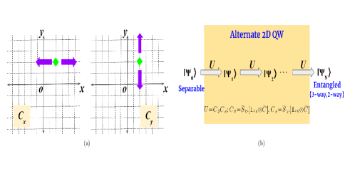
Figure 1: (a)Alternate quantum walk wherein after a coin operation particle (Green diamond) shifts either along $x$ or $y$-direction ($C_{x}$ or $C_{y}$ operation). (b) Alternate QW protocol for generating both 3-way and 2-way entanglement for a single-particle state, from an arbitrary separable initial state Eq. (1).

It is important to note that at an arbitrary time step $t=N$, the quantum state of the particle (2D quantum walker) has the following general form:

$$\ket{\psi_{N}}=U^{N}\ket{\psi_{i}}=\sum_{i,j}[h_{i,j}^{(N)}\ket{i_{x},j_{y},0_{c}}+v_{i,j}^{(N)}\ket{i_{x},j_{y},1_{c}}],$$ (5)

where, $h_{i,j}^{(N)}$ and $v_{i,j}^{(N)}$ are respectively the normalized complex amplitudes of the states $\ket{i_{x},j_{y},0_{c}}$ and $\ket{i_{x},j_{y},1_{c}}$. These are functions of the intial state parameters $\{\theta,\phi\}$ and coin operator parameters $\{\alpha,\beta,\gamma\}$. On applying the coin (Eq. (2)), the particle can shift to either $x$ or $y$ direction. Consequently, the particle’s state at the next time-step ($t=N+1$) will be,

$$\begin{split}\ket{\psi_{N+1}}=&\sum_{i,j}[h_{i-1,j-1}^{(N+1)}\ket{(i-1)_{x},(j-1)_{y},0_{c}}\\ &+h_{i+1,j-1}^{(N+1)}\ket{(i+1)_{x},(j-1)_{y},0_{c}}\\ &+v_{i-1,j+1}^{(N)}\ket{(i-1)_{x},(j+1)_{y},1_{c}}\\ &+v_{i+1,j+1}^{(N)}\ket{(i+1)_{x},(j+1)_{y},1_{c}}],\end{split}$$ (6)

where, $h_{i-1,j-1}^{(N+1)}=\cos{\alpha}(h_{i,j}^{(N)}\cos{\alpha}+v_{i,j}^{(N)}e^{i\beta}\sin{\alpha})$, $h_{i+1,j-1}^{(N+1)}=e^{i\beta}\sin{\alpha}(h_{i,j}^{(N)}e^{i\gamma}\sin{\alpha}-v_{i,j}^{(N)}e^{i(\beta+\gamma)}\cos{\alpha}),\;v_{i-1,j+1}^{(N+1)}=e^{i\gamma}\sin{\alpha}(h_{i,j}^{(N)}\cos{\alpha}+v_{i,j}^{(N)}e^{i\beta}\sin{\alpha}),\;v_{i+1,j+1}^{(N+1)}=e^{i(\beta+\gamma)}\cos{\alpha}(v_{i,j}^{(N)}e^{i(\beta+\gamma)}\cos{\alpha}-h_{i,j}^{(N)}e^{i\gamma}\sin{\alpha})$.

The interlacing coefficients within the time evolved states shown in Eqs. (5-6) provide an indication that these states can exhibit single-particle entanglement between the two nonlocal DoF: $x$ and $y$ position, i.e., we identify it as nonlocal 2-way entanglement. We also see that we can have 3-way entanglement between coin, $x$ and $y$ DoF (see Fig. 1(b)).

We perform several simulations to find a wide range of spatial sequences comprising an arbitrary coin operator, which can generate nonlocal $xy$-entanglement as well as 3-way entanglement between the three DoF ($x,y$ and coin) from arbitrary separable initial states (Eq. (1)).

Measuring entanglement.– The amount of quantum correlations in the single-particle entangled state between its three DoF ($x,y$ and coin), i.e., the 3-way SPE as well as between its nonlocal DoF ($x,y$), i.e., the nonlocal 2-way SPE can be measured via the negativity monotone [31, 29, 30]. In this context, we first deal with generating 3-way entanglement and then the nonlocal 2-way entanglement in a single particle state evolving via the alternate 2D QW. The 3-way entanglement of the quantum particle can be quantified by the monotone: triple-$\pi$ or $\pi$-tangle [30, 29], i.e., $\pi_{xyc}$ and it is defined as $\pi_{xyc}=\frac{\pi_{x}+\pi_{y}+\pi_{c}}{3}$. Here, $\pi_{i}=N_{i|jk}^{2}-N_{ij}^{2}+N_{ik}^{2}$ where $N_{i|jk}=\frac{||\rho^{\text{T}_{i}}_{ijk}||-1}{2}$, $N_{ij}=\frac{||\rho^{\text{T}_{i}}_{ij}||-1}{2}$ with $i,j,k\in\{x,y,c\}$, and $\text{T}_{i}$ denotes partial transpose with respect to DoF $i$ while $||.||$ refers to matrix trace norm. The residual negativity values ($\pi_{i}$) satisfy the Coffman-Kundu-Wootters (CKW) type monogamy inequalities [30, 32], $N_{i|jk}^{2}\geq N_{ij}^{2}+N_{ik}^{2}$, i.e., $\pi_{i}=N_{i|jk}^{2}-N_{ij}^{2}+N_{ik}^{2}\geq 0$. Examples of QW states, Eq. (6), obeying the CKW-type inequalities, are given in Supplementary Material (SM) [33] Sec. I. The average of the $\pi$-tangle at fixed $\phi$ (where $\phi$ is a parameter in initial state Eq. (1)) is, $\pi_{av}=\langle\pi_{xyc}\rangle=\frac{1}{\pi}\int_{0}^{\pi}\;\pi_{xyc}\;d\theta$. In general, $\pi_{xyc},\pi_{av}\geq 0$ whereas $\pi_{xyc}=\pi_{av}=0$ for any biseparation (e.g., for the initial state Eq. (1)), i.e., in absence of genuine 3-way entanglement wherein the quantum correlations are shared between all three DoF ($x,y$, coin) of the quantum particle [30].

To quantify the degree of entanglement between the nonlocal $x$ and $y$ DoF of the particle (quantum walker), we use entanglement negativity ($N$) [34]. To compute $N$ at any QW-time-step $t$, we first take the partial trace of the time-evolved density operator $\rho_{xyc}=\ket{\psi(t)}\bra{\psi(t)}$ over the coin DoF, i.e., $\rho_{xy}=\text{Tr}_{c}(\rho_{xyc})$, which is a quantum mixed state. From the eigenvalues $\{\lambda_{i}:i\in[1,(2t+1)^{2}]\}$ of the partial transpose (with respect to $x$ or $y$ DoF) of the reduced density matrix $\rho_{xy}$, we find the entanglement negativity, $N=\sum_{i=1}^{(2t+1)^{2}}\frac{|\lambda_{i}|-\lambda_{i}}{2}$.

Non-zero and positive $N$ values refer to entangled states, and for any separable or non-entangled state like the initial state given by Eq. (1), $N=0$. With a fixed $\phi$, average negativity is, $N_{av}=\langle N\rangle=\frac{1}{\pi}\int_{0}^{\pi}\;N\;d\theta$, and clearly, for a separable initial state (say, Eq. (1)), $N_{av}=0$.

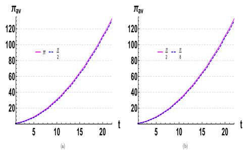
Figure 2: Three-way entanglement $\pi_{av}$ vs time steps($t$) for spatial evolution sequences: (a) $M1_{x}M1_{y}...$ for arbitrary separable initial state (Eq. (1)) with $\phi=\pi,\frac{\pi}{2}$; (b) $M2_{x}M2_{y}...$ for an arbitrary separable initial state with $\phi=\frac{\pi}{8},\frac{\pi}{2}$. Note that at all time steps, $M1_{x}M1_{y}$ with $\phi=\pi$ and $M2_{x}M2_{y}$ with $\phi=\frac{\pi}{2}$ yield the best values for 3-way entanglement among the cases we have studied.

3-way entanglement generation.– A quantum state of the particle (quantum walker) having 3-way entanglement (i.e., nonzero $\pi$-tangle) is not separable with respect to any bi-partition of the DoF. One can design quantum coin operators corresponding to different $\phi$ (phase parameter of the initial state) values that generate the maximum possible 3-way entanglement for the alternate 2D QW. Two such evolution operators (see, Eq. 4) are, $M1_{x}M1_{y},$ with $\phi=0,\pi,2\pi$ and $M2_{x}M2_{y}$ with $\phi=\frac{\pi}{2},\frac{3\pi}{2}$. Coin $\hat{M1}=\hat{C}(\alpha=\frac{5\pi}{16},\beta=\frac{\pi}{2},\gamma=\frac{\pi}{2})$, while coin $\hat{M2}=\hat{C}(\alpha=\frac{5\pi}{16},\beta=\pi,\gamma=\frac{\pi}{4})$. For evolution up to time step $t=22$, Fig. 2(a) shows the generated 3-way SPE for evolution sequences, $M1_{x}M1_{y}...$ with initially separable states Eq. (1) and $\phi=\pi,\frac{\pi}{2}$, while Fig. 2(b) depicts the 3-way SPE for evolution sequence $M2_{x}M2_{y}...$ with the same initial state (Eq. (1)) with $\phi=\frac{\pi}{2},\frac{\pi}{8}$. We clearly see from Fig. 2 that $M1_{x}M1_{y}$ gives maximal average $\pi$-tangle for $\phi=\pi$, whereas $M2_{x}M2_{y}$ gives the best results for $\phi=\frac{\pi}{2}$. Details regarding the simulations and the coins used to achieve maximal 3-way entanglement ($\pi_{av}$) in alternate 2D QW as a function of initial state parameters are provided in SM Sec. II [33]. The above-mentioned coins ($M1,\;M2$) are two of the numerous optimal coins (best entangling coins obtained from the simulations) that can generate maximal 3-way entanglement in 2D QW setups; see SM Sec. II and Table I [33]. The evolution $M1_{x}M1_{y}$ with the initial state parameter $\phi=\pi$ yields $\pi_{av}=2.0656\;(\text{at }t=2),30.6639\;(\text{at }t=10),132.5407\;(\text{at }t=22)$, whereas $M2_{x}M2_{y}$ with the state parameter $\phi=\frac{\pi}{2}$ yields $\pi_{av}=2.0656\;(\text{at }t=2),30.6639\;(\text{at }t=10),132.5407\;(\text{at }t=22)$, see Fig. 2

Further, in Fig. 3(a), we show the amount of 3-way SPE $\pi_{xyc}$ generated by both the evolution operators: $M1_{x}M1_{y},\;M2_{x}M2_{y}$ (with corresponding optimal $\phi$ values), at $t=15$ as a function of initial state parameter $\theta$ (which goes from 0 to $\pi$ in steps of $\frac{\pi}{32}$). This $\theta$-tuning reveals that for $\phi=\pi$ and $\theta=\frac{\pi}{2}$, the sequence $M1_{x}M1_{y}...$ yields maximum possible 3-way SPE with $\pi_{xyc}=69.0024$ (at $t=15$). At $\phi=\frac{\pi}{2}$ and $\theta=\frac{\pi}{2}$, the sequence $M2_{x}M2_{y}...$ yields maximum possible 3-way SPE with $\pi_{xyc}=69.0024$ again. For more analysis on maximal 3-way SPE generating evolution sequences, see SM Sec. II.

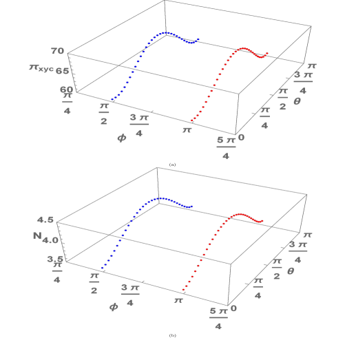
Figure 3: (a) 3-way entanglement ($\pi_{xyc}$) between $x,y$ and coin DoF vs the initial state parameter $\theta$ for spatial evolution sequences: $M1_{x}M1_{y}$ for the phase variable (of the initial state) $\phi=\pi$, and $M2_{x}M2_{y}$ for $\phi=\frac{\pi}{2}$ at time step $t=15$; (b) Nonlocal 2-way entanglement ($N$) between $x,y$ DoF vs the initial state parameter $\theta$ for spatial evolution sequences: $G1_{x}G1_{y}$ for the phase variable (of the initial state) $\phi=\pi$, $G2_{x}G2_{y}$ for $\phi=\frac{\pi}{2}$ at time step $t=15$.

Nonlocal 2-way $xy$-entanglement generation.– One can form numerous coin operators for arbitrary initial state $\phi$ values to generate maximum possible entanglement (SPE) between the nonlocal ($x,y$) DoF of the particle that evolves via the alternate 2D QW. Two distinct coin operators from Eq. (2), which generate maximum possible nonlocal $xy$ SPE are, $G1=\hat{C}(\alpha=\frac{19\pi}{16},\beta=\frac{\pi}{2},\gamma=\frac{\pi}{2})$ with $\phi=0,\pi$ and $G2=\hat{C}(\alpha=\frac{19\pi}{16},\beta=\pi,\gamma=\frac{\pi}{16})$ with $\phi=\frac{\pi}{2},\frac{3\pi}{2}$. See SM Sec. II for details on our simulations to find such coins. We denote the evolution operators involving these coins (Eq. (4)) to be $G1_{x}G1_{y}$ and $G2_{x}G2_{y}$.

Figure 4: Average nonlocal 2-way entanglement ($N_{av}$) between $x,y$ DoF vs time steps($t$) for spatial evolution sequences: (a) $G1_{x}G1_{y}...$ for the arbitrary separable initial state with $\phi=\pi,\frac{5\pi}{8}$, (b) $G2_{x}G2_{y}...$ for arbitrary separable initial state with $\phi=\frac{\pi}{8},\frac{\pi}{2}$. Note that $G1_{x}G1_{y}$ and $G2_{x}G2_{y}$ yield maximum 2-way entanglement respectively for $\phi=\pi$ and $\phi=\frac{\pi}{2}$.

Fig. 4 shows the average negativity ($N_{av}$) generated via the evolution $G1_{x}G1_{y}$ with $\phi=\pi,\frac{5\pi}{8}$ and $G2_{x}G2_{y}$ with $\phi=\frac{\pi}{8},\frac{\pi}{2}$. The spatial evolution sequences $G1_{x}G1_{y}...\;,G2_{x}G2_{y}...$ yield maximal average entanglement negativity respectively for $\phi=\pi$ and $\phi=\frac{\pi}{2}$, see Fig. 4, as one expects from the simulation (see, SM Sec. II [33]). Specifically, at time steps $t=2,10,22$, the sequence $G1_{x}G1_{y}$ for $\phi=\pi$ yields corresponding $N_{av}=0.4290,2.7089,5.9950$, while the sequence $G2_{x}G2_{y}$ for $\phi=\frac{\pi}{2}$ yields almost the same values as $G1_{x}G1_{y}$, see also SM Sec. II for more such optimal coins [33].

Furthermore, in Fig. 3(b), we show the amount of nonlocal 2-way entanglement $N$ generated by both the spatial evolution sequences at $t=15$ as a function of initial state parameter $\theta$ (which goes from 0 to $\pi$ in steps of $\frac{\pi}{32}$). This reveals that at $\phi=\pi$ and $\theta=\frac{\pi}{2}$, the sequence $G1_{x}G1_{y}...$ yields maximum nonlocal 2-way ($xy$) SPE with $N=4.4429$. Similarly, at $\phi=\frac{\pi}{2}$ and $\theta=\frac{\pi}{2}$, the spatial sequence $G2_{x}G2_{y}...$ also yields the same maximum nonlocal 2-way ($xy$) SPE with $N=4.4429$.

Remarks.– The above numerical simulations and analysis with the most general initial state (Eq. 1) yield numerous coin operators corresponding to certain phase values ($\phi$), which can generate a maximum amount of entanglement between all three ($x,y$ and coin) or the nonlocal ($x,y$) degrees of freedom of the single quantum particle evolving via the alternate 2D QW dynamics. For more coin evolution sequences like $M1_{x}M1_{y},\;M2_{x}M2_{y}$ for 3-way SPE and $G1_{x}G1_{y},\;G2_{x}G2_{y}$ for 2-way SPE and the numerical optimization details, see SM Sec. II [33]. The scheme also predicts at what specific value of state parameters $\phi$ and $\theta$, one can obtain maximum entanglement with the optimal coin evolution sequences such as $M1_{x}M1_{y},\;M2_{x}M2_{y}$ for 3-way SPE and $G1_{x}G1_{y},\;G2_{x}G2_{y}$ for nonlocal 2-way SPE. This contributes towards a state-of-art optimum entanglement generating protocol via alternate 2D QW. In addition, by tuning the parameters $\phi$ and $\theta$ of the initial state, one obtains controlled entanglement dynamics via the alternate 2D QW setup.

Summary with outlook.– Herein, we develop a framework to generate and control genuine 3-way SPE (involving all $x,y,c$ DoF) as well as nonlocal 2-way SPE (involving $x$ and $y$ DoF) of any quantum particle evolving via a generalised alternate 2D QW with resource-saving single-qubit coins. The analytical-cum-numerical investigations predict numerous optimal quantum coin operators corresponding to particular values of the initial state ($\phi$), which yield maximal 3-way and 2-way nonlocal SPE for the particle evolving from an initial separable state via the QW setup (also see SM Sec. II). The optimal coins for 3-way SPE also yield a large amount of 2-way SPE, which implies that the generated 3-way SPE states can be predominantly of W-type [11]. A comparison of our work with other relevant works [17, 16, 6] is given in SM Sec. III [33]. Our Letter, apart from opening an unprecedented avenue for generating 3-way entanglement at the single particle level, outperforms the other existing schemes in terms of overall resource-saving architecture and yielding high values of nonlocal 2-way entanglement.

Our proposal can be experimentally realized with photons [35] wherein the photon’s path, OAM and polarization are mapped respectively into the walker’s $x,\;y$ and coin DoF. This can also be adapted to other experimental setups that can realize 2D-quantum walks. This scheme contributes towards state-of-art in generating genuine 3-way entangled and 2-way entangled single-particle states, which are crucial for large-scale QI processing. Our scheme of designing and controlling entanglement dynamics via quantum walks have potential applications in entanglement protocols for quantum information processing [1], entanglement-based quantum cryptography [36], QW-based quantum algorithms [37], realization of non-Markovian quantum channels [38] and studying the dynamics of open quantum systems.

Supplementary Material for ”Designing three-way entangled and nonlocal two-way entangled single particle states via alternate quantum walks”

Dinesh Kumar Panda^1,2,  Colin Benjamin^1,2

¹School of Physical Sciences, National Institute of Science Education and Research Bhubaneswar, Jatni 752050, India

²Homi Bhabha National Institute, Training School Complex, Anushaktinagar, Mumbai 400094, India

Herein, we provide a more detailed derivation of the validity of the CKW-type monogamy inequalities [32, 30] for the 2D quantum walk states in Sec. I. In Sec. II, we give details of simulations to obtain coin and initial state parameters that yield a maximal amount of 3-way and nonlocal 2-way single-particle entanglement (SPE). Further details on 3-way and 2-way SPE generation via the optimal coins designed via the simulations are included, also. Sec. III provides a comparison of our work with other relevant proposals to generate nonlocal 2-way SPE.

I CKW-type inequalities in single-particle entanglement via alternate 2D quantum walks

The 3-way entanglement of the quantum particle evolving via the alternate 2D QW (as discussed in the main text) can be quantified by the monotone triple-$\pi$ or $\pi$-tangle [30, 29], i.e., $\pi_{xyc}$. As in the main text (Eq. (1)), the initial separable state of the particle (quantum walker) at time-step $t=0$ is $\ket{\psi_{i}}=\ket{\psi(t=0)}$, i.e.,

$$\ket{\psi_{i}}=\ket{0_{x},0_{y}}\otimes[\cos(\frac{\theta}{2})\ket{0_{c}}+e^{i\phi}\sin(\frac{\theta}{2})\ket{1_{c}}],$$ (7)

where $\theta\in[0,\pi]$ and phase $\phi\in[0,2\pi)$. The particle evolves via the evolution operator,

$$\begin{split}U(t)=\hat{S}_{y}.[\mathbb{1}_{xy}\otimes\hat{C}].\hat{S}_{x}.[\mathbb{1}_{xy}\otimes\hat{C}]\;,\end{split}$$ (8)

where $\hat{C}=\hat{C}(\alpha(t),\beta(t),\gamma(t))=\begin{pmatrix}\cos{\alpha}&e^{i\beta}\sin{\alpha}\\ \sin{\alpha}e^{i\gamma}&-e^{i(\beta+\gamma)}\cos{\alpha}\end{pmatrix}$ is the coin operator and

$$\hat{S_{x}}= \sum_{j=-\infty}^{\infty}\{\ket{(j-1)_{x}}\bra{j_{x}}\otimes\mathbb{1}_{y}\otimes\ket{0_{c}}\bra{0_{c}}+\ket{(j+1)_{x}}\bra{j_{x}}\otimes\mathbb{1}_{y}\otimes\ket{1_{c}}\bra{1_{c}}\},$$ (9)

$$\hat{S_{y}}= \sum_{j=-\infty}^{\infty}\{\mathbb{1}_{x}\otimes\ket{(j-1)_{y}}\bra{j_{y}}\otimes\ket{0_{c}}\bra{0_{c}}+\mathbb{1}_{x}\otimes\ket{(j+1)_{y}}\bra{j_{y}}\otimes\ket{1_{c}}\bra{1_{c}}\},$$

are the shift operators that move the walker along $x$ and $y$ directions. $\mathbb{1}_{x}$ and $\mathbb{1}_{y}$ are identity operators respectively in $x$ and $y$ position Hilbert-spaces. The evolution operator (Eq. 8) for each QW time-step is denoted by, $C_{x}C_{y}$, with $C_{x}=\hat{S}_{x}.[\mathbb{1}_{xy}\otimes\hat{C}]$ and $C_{y}=\hat{S}_{y}.[\mathbb{1}_{xy}\otimes\hat{C}]$.

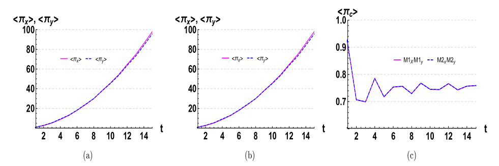
Figure 5: CKW-type inequalities for quantum states in alternate 2D QWs: (a) Average residual negativities ($\langle\pi_{x}\rangle$, $\langle\pi_{y}\rangle$) vs time steps($t$) for spatial evolution sequence $M1_{x}M1_{y}...$ for an separable initial state Eq. (7) with $\phi=\pi$; (b) Average residual negativities ($\langle\pi_{x}\rangle$, $\langle\pi_{y}\rangle$) vs time steps($t$) for spatial evolution sequence $M2_{x}M2_{y}...$ for separable initial state Eq. (7) with $\phi=\frac{\pi}{2}$; (c) Average residual negativity ($\langle\pi_{c}\rangle$) vs time steps($t$) for spatial evolution sequences, $M1_{x}M1_{y}...$ for arbitrary separable initial state Eq. (7) with $\phi=\pi$ and $M2_{x}M2_{y}...$ for the separable initial state with $\phi=\frac{\pi}{2}$.

For the particle’s states at any QW-time-step $t$, the following residual negativity values need to satisfy the Coffman-Kundu-Wootters (CKW) type monogamy inequalities [30, 32]: $N_{i|jk}^{2}\geq N_{ij}^{2}+N_{ik}^{2}$, where $N_{i|jk}=\frac{||\rho^{\text{T}_{i}}_{ijk}-1||}{2}$, $N_{ij}=\frac{||\rho^{\text{T}_{i}}_{ij}-1||}{2}$ with $i,j,k\in\{x,y,c\}$, and $\text{T}_{i}$ denotes partial transpose with respect to DoF $i$ while $||.||$ refers to matrix trace norm. This is equivalent to,

$$\pi_{x}= N_{x|yc}^{2}-N_{xy}^{2}+N_{xc}^{2}\geq 0,\;\pi_{y}= N_{y|cx}^{2}-N_{yc}^{2}+N_{yx}^{2}\geq 0,\;\text{and }\pi_{c}= N_{c|xy}^{2}-N_{cx}^{2}+N_{cy}^{2}\geq 0,$$ (10)

i.e., $\pi_{x},\pi_{y},\pi_{c}$ are non-negative. Thus, at a fixed $\phi$-value, the $\theta$-average values $\langle\pi_{i}\rangle=\frac{1}{\pi}\int_{0}^{\pi}\;\pi_{i}\;d\theta$ would follow the inequalities $\langle\pi_{i}\rangle\geq 0$, i.e., $\langle\pi_{i}\rangle$ is non-negative for all $i\in\{x,y,c\}$ at any $t$. For examples of quantum states generated via the alternate 2D quantum walk (QW) that satisfies the inequalities, see Fig. 5. In Fig. 5, the single-particle states are generated via two QW evolution sequences: $M1_{x}M1_{y}...$ and $M2_{x}M2_{y}...$ with state phase parameter $\phi=\pi$ or $\phi=\frac{\pi}{2}$. Fig. 5(a) and (b) respectively show the plots of $\langle\pi_{x}\rangle$, $\langle\pi_{y}\rangle$ for the the sequences $M1_{x}M1_{y}...$ and $M2_{x}M2_{y}...$ , as a function of time step $t$. In Fig. 5(c) we show the plot of $\langle\pi_{c}\rangle$ for the sequences $M1_{x}M1_{y}...$ and $M2_{x}M2_{y}...$ , as a function of time step $t$. Clearly, the values $\langle\pi_{i}\rangle$ are non-negative for all $i\in\{x,y,c\}$ at any time step $t$. This shows that QW states do satisfy the CKW-type inequalities.

The 3-way entanglement measure, $\pi$-tangle is defined as $\pi_{xyc}=\frac{\pi_{x}+\pi_{y}+\pi_{c}}{3}$ and its average at fixed $\phi$ is, $\pi_{av}=\langle\pi_{xyc}\rangle=\frac{1}{\pi}\int_{0}^{\pi}\;\pi_{xyc}\;d\theta$. The validity of CKW-type inequalities ($\pi_{x},\pi_{y},\pi_{c}\geq 0$) implies that, in general, the 3-way entanglement measure $\pi_{xyc}\geq 0$. Note that $\pi_{xyc}=\pi_{av}=0$ for any biseparation, i.e., in the absence of genuine 3-way entanglement. For genuine 3-way entanglement, the quantum correlations are shared between all three DoF ($x,y$, coin) of the quantum particle [30]. The evolution sequences $M1_{x}M1_{y}...$ and $M2_{x}M2_{y}...$ generate genuine 3-way SPE ($\pi_{av}>0$) at all time-steps as shown in the main, see Fig. 2.

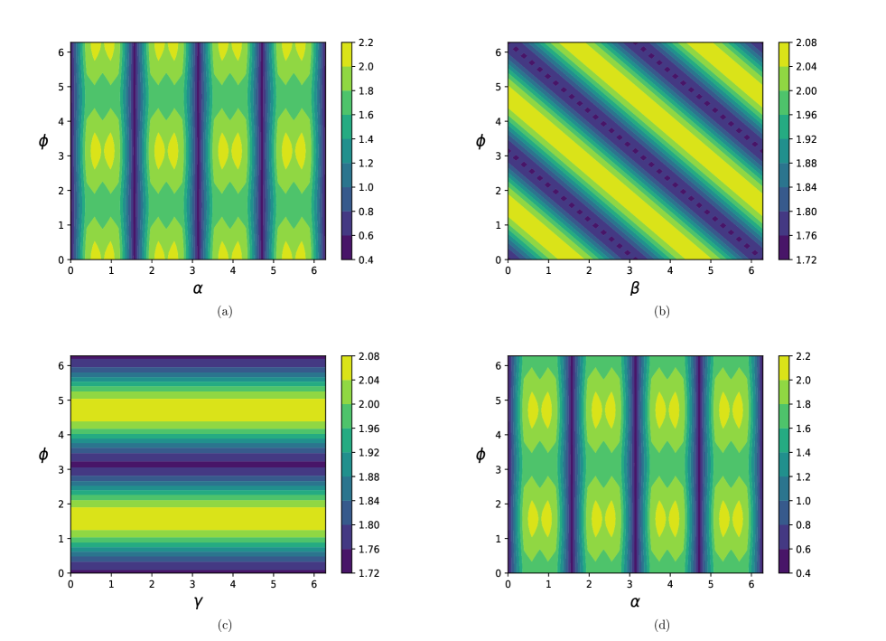
Figure 6: 3-way entanglement $\pi_{av}$ as a function of initial state parameter $\phi$ and coin parameters: (a) $\alpha$ with $(\beta=\frac{\pi}{2},\gamma=\frac{\pi}{2})$, (b) $\beta$ with $(\alpha=\frac{3\pi}{16},\gamma=\frac{\pi}{2})$, (c) $\gamma$ with $(\alpha=\frac{3\pi}{16},\beta=\pi)$, (d) $\alpha$ with $(\beta=\pi,\gamma=\frac{\pi}{8})$ at time step $t=2$. In all subplots, each parameter from the set $\{\phi,\alpha,\beta,\gamma\}$ is varied from 0 to $2\pi$ in steps of $\frac{2\pi}{32}$.

II Simulations to achieve maximal 3-way and nonlocal 2-way entanglement via single-particle alternate 2D quantum walk

II.1 3-way entanglement

Herein, we discuss the numerical experiments on the average 3-way entanglement (SPE) ($\pi_{av}$) as a function of the evolution-operator and initial state parameters. The average is taken over an initial state parameter $\theta$, i.e., $\pi_{av}=\frac{1}{\pi}\int_{0}^{\pi}\pi_{xyc}\;d\theta$ at $t=2$. Post analysing the results shown in Fig. 6, the values of the parameters at which the $\pi_{av}$ attains maximum are given in Table 1. One can observe that numerous optimal coin operators can be formed from Table 1, which yield a large $\pi$-tangle (3-way SPE). Noteworthy that increasing $t$ automatically leads to an increase in dimensions of $x$ and $y$ DoF. This causes the residual negativity values ($\pi_{x}$ and $\pi_{y}$) to increase with $t$, see Ref. [6] and Fig. 5. Investigating the QW evolution to generate 3-way SPE with a general initial state (Eq. (7)) and general coin (Eq. (2)) is computationally very costly and challenging. These two reasons lead us to optimize for the time-step $t=2$ in generating maximal 3-way SPE in the QW evolution. This is shown in Fig. 5, and the results can be further utilized at large $t$ to generate maximal values of 3-way SPE ($\pi_{av}$).

From the numerical results shown in Fig. 6, one can form numerous optimal coins (or evolution sequences) corresponding to particular $\phi$ values, which give rise to maximum possible $\pi_{av}$ value. For example, the coins $\hat{M1}=\hat{C}(\alpha=\frac{5\pi}{16},\beta=\frac{\pi}{2},\gamma=\frac{\pi}{2})$ obtained from Fig. 6(a), $\hat{M3}=\hat{C}(\alpha=\frac{5\pi}{16},\beta=\frac{6\pi}{16},\gamma=\frac{\pi}{2})$ from Fig. 6(b), $\hat{M2}=\hat{C}(\alpha=\frac{5\pi}{16},\beta=\pi,\gamma=\frac{\pi}{4})$ from Fig. 6(c), and $\hat{M4}=\hat{C}(\alpha=\frac{11\pi}{16},\beta=\pi,\gamma=\frac{\pi}{8})$ from Fig. 6(d) yield maximum $\pi_{av}$ value, e.g., $\pi_{av}=2.0656$ at $t=2$, see Table 1. In the main text Fig. 2, we plotted the three-way SPE generated as a function of time steps ($t$) for the coins $\hat{M1}$ and $\hat{M2}$. In Fig. 7, see 3-way SPE generated as a function of $t$ via the coins $\hat{M3}$ and $\hat{M4}$.

All sets of coin operators, along with corresponding $\phi$ values which give rise to maximum $\pi_{av}$ value, are provided in Table 1.

Coin operator	Initial state phase $\phi$ and coin parameters ($\alpha,\beta,\gamma$) in units of $\frac{2\pi}{32}$	Maximum 3-way
$\hat{C}(\alpha,\beta=\frac{\pi}{2},\gamma=\frac{\pi}{2})$	$\phi=0,\alpha\in\{3,5,11,13,19,21,27,29\};\;\phi=16,\alpha\in\{3,5,11,13,19,21,27,29\}$	$\pi_{av}$=2.0656
	$\phi=32,\alpha\in\{3,5,11,13,19,21,27,29\}$
$\hat{C}(\alpha=\frac{5\pi}{16},\beta,\gamma=\frac{\pi}{2})$	$\phi=j,\beta\in\{8-j,24-j\}|j\in[0,8]\cap\mathbb{Z};\;\phi\in\{8,24\},\beta=32$	$\pi_{av}$=2.0656
	$\phi=9+j,\beta\in\{31-j,15-j\}|j\in[0,15]\cap\mathbb{Z};\;\phi=25+j,\beta\in\{15-j,31-j\}|j\in[0,7]\cap\mathbb{Z}$
$\hat{C}(\alpha=\frac{5\pi}{16},\beta=\pi,\gamma)$	$\phi=8,\gamma\in[0,32]\cap\mathbb{Z}$	$\pi_{av}$=2.0656
	$\phi=24,\gamma\in[0,32]\cap\mathbb{Z}$
$\hat{C}(\alpha,\beta=\pi,\gamma=\frac{\pi}{8})$	$\phi=8,\alpha\in\{3,5,11,13,19,21,27,29\}$	$\pi_{av}$=2.0656
	$\phi=24,\alpha\in\{3,5,11,13,19,21,27,29\}$

Table 1: Coin operators and initial states from simulation results of Fig. 6, for maximum 3-way entanglement ($\pi_{av}$).

Figure 7: Three-way entanglement ($\pi_{av}$) vs time steps($t$) for spatial evolution sequences: (a) $M3_{x}M3_{y}...$ for arbitrary separable initial state Eq. (7) with $\phi=\frac{\pi}{8},\frac{\pi}{2}$; (b) $M4_{x}M4_{y}...$ for the arbitrary separable initial state with $\phi=\frac{\pi}{2},\frac{\pi}{8}$.

II.2 Nonlocal 2-way entanglement

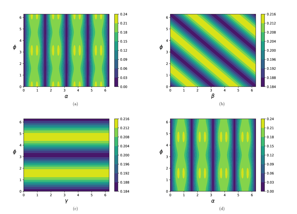
Figure 8: Nonlocal entanglement ($N_{av}$) between $x,y$ DoF as a function of initial state parameter $\phi$ and coin parameters: (a) $\alpha$ with $(\beta=\frac{\pi}{2},\gamma=\frac{\pi}{2})$, (b) $\beta$ with $(\alpha=\frac{19\pi}{16},\gamma=\frac{\pi}{2})$, (c) $\gamma$ with $(\alpha=\frac{19\pi}{16},\beta=\pi)$, (d) $\alpha$ with $(\beta=\pi,\gamma=\frac{\pi}{8})$ at time step $t=2$. In all subplots, each parameter from the set $\{\phi,\alpha,\beta,\gamma\}$ is varied from 0 to $2\pi$ in steps of $\frac{2\pi}{128}$, resulting in a total 65536 combinations of separable initial states and coin operators to generate nonlocal $xy$-entanglement.

Herein, we discuss the simulations in Fig. 8 to achieve a maximal value for the nonlocal 2-way single-particle entanglement between the nonlocal $x$ and $y$-DoF of the particle (e.g., the SPE between the photon’s internal OAM and its external path, i.e., the spatial trajectories). The particle evolves via the alternate 2D QW dynamics from a separable initial state given in Eq. 7. The nolocal 2-way entanglement is quantified by entanglement negativity $N$, as discussed in the main (Page-3) and the average negativity, $N_{av}=\langle N\rangle=\frac{1}{\pi}\int_{0}^{\pi}\;N\;d\theta$. Pertaining to the relation given in Eqs. (5) and (6) of main, Fig. 8 shows the entanglement negativity $N_{av}$ as a function of initial state parameter $\phi$ and coin parameters at time step $t=2$. Note that due to the increase of dimensions of $x$ and $y$ DoF, with an increase in QW time steps, the negativity increases with time steps ($t$), see Ref. [6]. In addition, investigating 2D QW schemes to generate nonlocal SPE with a general initial state (Eq. (7)) and general coin (Eq. (2)) is computationally very costly and challenging. This leads us to optimize for the time-step $t=2$ in generating the nonlocal $xy$-entanglement as shown in Fig. 8, and its results can be utilized for large $t$ to generate a maximal amount of entanglement as well. In all the subplots of Fig. 8, each parameter from the set $\{\phi,\alpha,\beta,\gamma\}$ is varied between 0 and $2\pi$ in steps of $\frac{2\pi}{128}$, resulting in a total 65536 combinations of separable initial states and coin operators to generate nonlocal $xy$-entanglement and then determine the maximal values. In Fig. 8(a), the maximization of $N_{av}$ with respect to $\phi$ and coin parameter $\alpha$ is obtained with $(\beta=\frac{\pi}{2},\gamma=\frac{\pi}{2})$. This yields a set of coin operators which with a certain initial state, generate optimum $N_{av}$ value, i.e., 0.429. Similarly, Fig. 8(b) with $\beta$ $(\alpha=\frac{19\pi}{16},\gamma=\frac{\pi}{2})$, yields another set of coin operators with corresponding $\phi$ values (initial states) to generate the same optimum value $N_{av}=0.429$. Furthermore, Fig. 8(c) with $(\alpha=\frac{19\pi}{16},\beta=\pi)$ give rise to another set of coin operators along with $\phi$ values to get optimum $N_{av}=0.429$. Here, it is interesting to observe that specific to any $\phi$ value, the entanglement $N_{av}$ is independent of the coin parameter $\gamma$. Fig. 8 (d) involves optimization with $\alpha$ at $\beta=\pi,\gamma=\frac{\pi}{8}$ and yields a large set of coin operators each of which generate maximum $N_{av}=0.429$ corresponding to certain $\phi$ values, at time step $t=2$. All these sets of coin operators along with corresponding $\phi$ values which give rise to maximum $N_{av}$ values, are provided in Table 2. From Fig. 8 or Table 2, one can form numerous coin operators along with $\phi$ values (i.e., phase parameter of the initial state) to generate maximal values of entanglement between the nonlocal DoF of the particle.

Coin operator	Initial state phase $\phi$ and coin parameters ($\alpha,\beta,\gamma$) in units of $\frac{2\pi}{128}$	Maximum 2-way
$\hat{C}(\alpha,\beta=\frac{\pi}{2},\gamma=\frac{\pi}{2})$	$\phi=0,\alpha\in\{12,20,44,52,76,84,108,116\};\;\phi=64,\alpha\in\{12,20,44,52,76,84,108,116\}$	$N_{av}=0.429$
	$\phi=128,\alpha\in\{12,20,44,52,76,84,108,116\}$
$\hat{C}(\alpha=\frac{19\pi}{16},\beta,\gamma=\frac{\pi}{2})$	$\phi=128-j,\beta\in\{96+j,32+j\}|j\in[0,32]\cap\mathbb{Z};\;\phi\in\{96,32\},\beta=0$	$N_{av}=0.429$
	$\phi=96-j,\beta\in\{j,64+j\}|j\in[1,64]\cap\mathbb{Z};\;\phi=32-j,\beta\in\{96+j,64+j\}|j\in[1,32]\cap\mathbb{Z}$
$\hat{C}(\alpha=\frac{19\pi}{16},\beta=\pi,\gamma)$	$\phi=32,\gamma\in[0,128]\cap\mathbb{Z}$	$N_{av}=0.429$
	$\phi=96,\gamma\in[0,128]\cap\mathbb{Z}$
$\hat{C}(\alpha,\beta=\pi,\gamma=\frac{\pi}{8})$	$\phi=32,\alpha\in\{12,20,44,52,76,84,108,116\}$	$N_{av}=0.429$
	$\phi=96,\alpha\in\{12,20,44,52,76,84,108,116\}$

Table 2: Coin operators and initial states from simulation results of Fig. 6, for maximum 2-way nonlocal ($xy$) entanglement.

For instance, we design the coin operators, $\hat{G1}=\hat{C}(\alpha=\frac{19\pi}{16},\beta=\frac{\pi}{2},\gamma=\frac{\pi}{2})$ with $\phi=\pi,0$ from Fig. 8(a), $\hat{G3}=\hat{C}(\alpha=\frac{19\pi}{16},\beta=\frac{11\pi}{8},\gamma=\frac{\pi}{2})$ with $\phi=\frac{\pi}{8},\frac{9\pi}{8}$ from Fig. 8(b), $\hat{G2}=\hat{C}(\alpha=\frac{19\pi}{16},\beta=\pi,\gamma=\frac{\pi}{16})$ with $\phi=\frac{\pi}{2},\frac{3\pi}{2}$ from Fig. 8(c), and $\hat{G4}=\hat{C}(\alpha=\frac{5\pi}{16},\beta=\pi,\gamma=\frac{\pi}{8})$ with $\phi=\frac{\pi}{2},\frac{3\pi}{2}$ from Fig. 8(d) which yield maximum possible nonlocal 2-way SPE. We denote the evolution operators (Eq. (8)) involving these coins to be respectively $G1_{x}G1_{y},\;G3_{x}G3_{y},\;G2_{x}G2_{y}$ and $G4_{x}G4_{y}$.

These spatial evolution sequences $G1_{x}G1_{y},\;G3_{x}G3_{y},\;G2_{x}G2_{y}$ and $G4_{x}G4_{y}$, yield maximum possible value of average entanglement negativity $N_{av}$ (as per Fig. 8). See main Fig. 4 for 2-way SPE generation via the evolutions: $G1_{x}G1_{y},\;G2_{x}G2_{y}$ and Fig. 9 below for 2-way SPE generation via the evolutions: $G3_{x}G3_{x},\;G4_{x}G4_{y}$. The spatial evolution sequences $G3_{x}G3_{x}...,\;G4_{x}G4_{y}...$ yield maximal average entanglement negativity respectively for $\phi=\frac{\pi}{8}$ and $\phi=\frac{\pi}{2}$, as one expects from the simulations (Fig. 8).

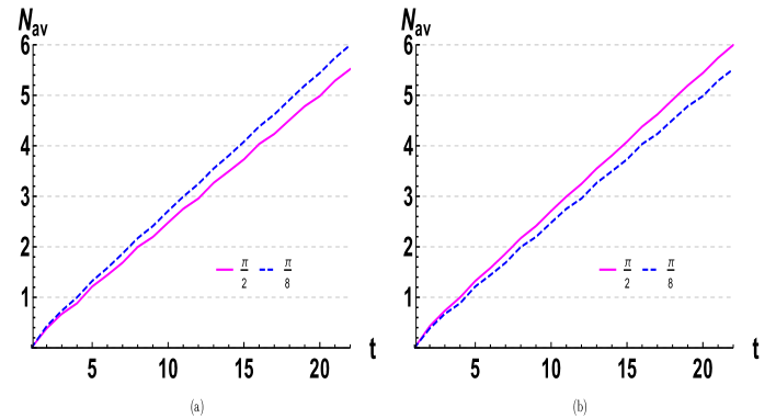
Figure 9: Nonlocal entanglement ($N_{av}$) between $x,y$ DoF vs time steps($t$) for spatial evolution sequences: $G3_{x}G3_{y}...$ for separable initial states (Eq. (7)) with $\phi\in\{\frac{\pi}{2},\frac{\pi}{8}\}$ and $G4_{x}G4_{y}...$ for the separable initial states with $\phi\in\{\frac{\pi}{2},\frac{\pi}{8}\}$.

III Comparison between single-particle entanglement generation approaches

It is to be noted that there is no report of any work on generating genuine 3-way entanglement (SPE) prior to this Letter. Apart from generating 3-way SPE states, this Letter reports the maximum possible values for the 3-way entanglement in a single quantum particle evolving via alternate 2D QW. We also achieve maximum possible nonlocal 2-way SPE for the particle. We now compare our results on nonlocal 2-way SPE with previous relevant works [6, 16, 17]. Ref. [17] considers a general initial state but only with a Hadamard coin to achieve the 2-way SPE generation. On the other hand, Ref. [6] discusses this considering a particular initial state with $\theta=\frac{\pi}{2}$ and $\phi=0$ , where each step in the QW involves the operation of a coin and its hermitian conjugate. Ref. [16] uses Hadamard coin along with a particular initial state with $\theta=\frac{\pi}{2}$ and $\phi=\pi$ to generate SPE. Our work provides a complete investigation of 2-way (and genuine 3-way) SPE generation considering both general initial state as well as arbitrary single-qubit coin operators. Fig. 10 shows the entanglement generated via the best entanglers from Refs. [6, 16, 17] vs. two of our optimal entanglers ($G1_{x}G1_{x}...$, $G2_{x}G2_{x}...$). One can clearly observe that our scheme outperforms these schemes in generating nonlocal 2-way SPE at all time steps ($t$). In particular, at time-step $t=25$, our scheme exceeds both the existing schemes. Moreover, our work, apart from giving a most general investigation, provides a more resource-saving avenue to generate SPE than Ref. [6]. The latter involves the use of a coin and its hermitian conjugate at each time step of the alternate QW, in contrary to our use of just a single coin. The similarities and comparisons between our work and the three relevant works are juxtaposed in Table 3.

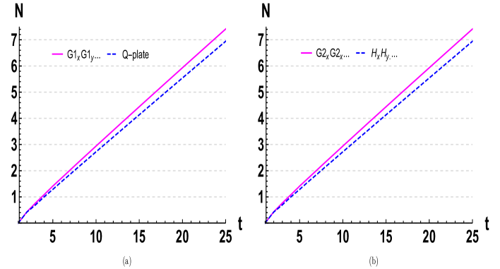
Figure 10: Nonlocal entanglement ($N_{xy}$) between $x,y$ DoF, up to 25 time steps ($t$), (a) for the spatial evolution sequence $G1_{x}G1_{y}...$ vs. optimal entangler of Ref. [6] (i.e., the q-plate coin evolution sequence) for initial state (Eq. (7)) with ($\theta=\frac{\pi}{2},\phi=0$); (b) for the spatial evolution sequence $G2_{x}G2_{y}...$ vs. optimal entangler of Refs. [17, 16] (i.e., $H_{x}H_{y}$ sequence), for initial state (Eq. (7)) with ($\theta=\frac{\pi}{2},\phi=\frac{\pi}{2}$). Note that at $t=1$, $N_{av}=0$ for all four evolution sequences.

Table 3: Comparison between nonlocal single-particle entanglement generating approaches

Properties$\downarrow$/Model$\rightarrow$	Alternate QW with spatial sequences (This paper)	Regular QW and Hadamard-coin alternate QW [16]	Alternate QW with Hadamard coin [17]	Modified Pauli QW Ref. [6]
Genuine 3-way entanglement generation	Yes, and we obtain maximal values via alternate 2D QW.	Not attempted.	Not attempted.	Not attempted.
Controlled nonlocal $xy$ entanglement Generation	Yes.	Not discussed.	Not achieved.	Not achieved.
Maximizing nonlocal SPE ($N$) over initial state parameters ($\theta,\phi$)	Yes, and we average results over $\theta$ values. Arbitrary coin operators are considered.	Not discussed.	Yes, but with only Hadamard coin (less than maximal).	Not discussed.
Maximizing nonlocal SPE ($N$) over coin parameters ($\alpha,\beta,\eta$)	Yes.	Not discussed.	Not discussed.	Partially discussed with a specific initial state.
Achieved nonlocal SPE (negativity) values	Large, e.g., $N=7.4104$ $\rightarrow$ $G1_{x}G1_{y}...$ at $(t=25,\phi=0,\theta=\frac{\pi}{2})$ $N=7.4104$ $\rightarrow$ $G2_{x}G2_{y}...$ at $(t=25,\phi=\frac{\pi}{2},\theta=\frac{\pi}{2})$ (Similar results via arbitrary coin operators from Table 2).	Best result is $N=6.9429$$\rightarrow$ $H_{x}H_{y}...$ at $(t=25,\phi=\frac{\pi}{2},\theta=\frac{\pi}{2})$.	Best result is $N=6.9429$$\rightarrow$ $H_{x}H_{y}...$ at $(t=25,\phi=\frac{\pi}{2},\theta=\frac{\pi}{2})$.	Best result is, $N=6.9429$$\rightarrow$$C_{x}C_{y}...$ at $(t=25,\phi=0,\theta=\frac{\pi}{2})$.

References

- [1] S. Azzini, S. Mazzucchi, V. Moretti, D. Pastorello, and L. Pavesi, Single-Particle Entanglement, Advanced Quantum Technologies 3, 2000014 (2020).
- [2] A. Gratsea, M. Lewenstein, and A. Dauphin, Generation of hybrid maximally entangled states in a one-dimensional quantum walk, Quantum Science and Technology 5, 025002 (2020).
- [3] Xiao-Xu Fang, Kui An, Bai-Tao Zhang, Barry C. Sanders, He Lu, Maximal coin-position entanglement generation in a quantum walk for the third step and beyond regardless of the initial state, Phys. Rev. A 107, 012433 (2023).
- [4] C. Vitelli, N. Spagnolo, F. Sciarrino, E. Santamato, and L. Marrucci, Joining the quantum state of two photons into one, Research in optical sciences, OSA Technical Digest, Paper QW3B.2 (Optical Society of America, Washington, DC, 2014).
- [5] C. H. Bennett and G. Brassard, Quantum cryptography: Public key distribution and coin tossing, Theor. Comput. Sci. 560, 7 (2014).
- [6] P. A. Ameen Yasir and C. M. Chandrashekar, Generation of hyperentangled states and two-dimensional quantum walks using J or q plates and polarization beam splitters, Phys. Rev. A 105, 012417 (2022).
- [7] Zhi-Hao Ma et al., Measure of genuine multipartite entanglement with computable lower bounds, Phys. Rev. A 83, 062325 (2011).
- [8] Zhi-Hua Chen et al., Improved lower bounds on genuine-multipartite-entanglement concurrence, Phys. Rev. A 85, 062320 (2012).
- [9] Li, M., Wang, J., Shen, S. et al. Detection and measure of genuine tripartite entanglement with partial transposition and realignment of density matrices. Sci Rep 7, 17274 (2017).
- [10] R. Raussendorf and H. J. Briegel, Phys. Rev. Lett. 86, 5188 (2001).
- [11] M. Blasone, F. Dell’Anno, S. De Siena, M. Di Mauro, and F. Illuminati, Multipartite entangled states in particle mixing, Phys. Rev. D 77, 096002 (2008).
- [12] Abhishek Kumar Jha, Supratik Mukherjee, and Bindu A. Bambah, Tri-partite entanglement in neutrino oscillations, Mod. Phys. Lett. A 36, 2150056 (2021).
- [13] Chao Zhang, Wen-Hao Zhang, Pavel Sekatski, Jean-Daniel Bancal, Michael Zwerger, Peng Yin, Gong-Chu Li, Xing-Xiang Peng, Lei Chen, Yong-Jian Han, Jin-Shi Xu, Yun-Feng Huang, Geng Chen, Chuan-Feng Li, and Guang-Can Guo, Certification of Genuine Multipartite Entanglement with General and Robust Device-Independent Witnesses, Phys. Rev. Lett. 129, 190503 (2022).
- [14] Beatrix C. Hiesmayr and Pawel Moskal, Genuine Multipartite Entanglement in the 3-Photon Decay of Positronium. Sci Rep 7, 15349 (2017).
- [15] Huan Cao, Simon Morelli, Lee A. Rozema, Chao Zhang, Armin Tavakoli, and Philip Walther, Genuine multipartite entanglement without fully controllable measurements, arXiv:2310.11946 [quant-ph] (2023).
- [16] C. Di Franco, M. Mc Gettrick, and Th. Busch, Mimicking the Probability Distribution of a Two-Dimensional Grover Walk with a Single-Qubit Coin, Phys. Rev. Lett. 106, 080502 (2011).
- [17] C. Di Franco, M. Mc Gettrick, T. Machida, and Th. Busch, Alternate two-dimensional quantum walk with a single-qubit coin, Phys. Rev. A 84, 042337
- [18] ] K. Eckert et al., Phys. Rev. A 72, 012327 (2005).
- [19] Dinesh Kumar Panda, B. Varun Govind, Colin Benjamin, Generating highly entangled states via discrete-time quantum walks with Parrondo sequences, Physica A: Statistical Mechanics and its Applications 608, 128256 (2022).
- [20] Rong Zhang et al., Maximal coin-walker entanglement in a ballistic quantum walk, Phys. Rev. A 105, 042216 (2022).
- [21] Dinesh Kumar Panda and Colin Benjamin, Recurrent generation of maximally entangled single-particle states via quantum walks on cyclic graphs, Phys. Rev. A 108, L020401 (2023).
- [22] A. Gratsea, F. Metz, and T. Busch, Universal and optimal coin sequences for high entanglement generation in 1D discrete time quantum walks, Journal of Physics A: Mathematical and Theoretical 53, 445306 (2020).
- [23] S. Li, H. Yan, Y. He, and H. Wang, Experimentally feasible generation protocol for polarized hybrid entanglement, Phys. Rev. A 98, 022334 (2018).
- [24] C. M. Chandrashekar, Disorder induced localization and enhancement of entanglement in one and two-dimensional quantum walks (2012), arXiv:1212.5984[quant-ph].
- [25] R. Vieira, E. P. M. Amorim, and G. Rigolin, Dynamically disordered quantum walk as a maximal entanglement generator, Phys. Rev. Lett. 111, 180503 (2013).
- [26] R. Vieira, E. P. M. Amorim, and G. Rigolin, Entangling power of disordered quantum walks, Phys. Rev. A 89, 042307 (2014).
- [27] D. Gross, S. T. Flammia, and J. Eisert, Most Quantum States Are Too Entangled To Be Useful As Computational Resources, Phys. Rev. Lett. 102, 190501 (2009).
- [28] Anders Karlsson and Mohamed Bourennane, Quantum teleportation using three-particle entanglement, Phys. Rev. A 58, 4394 (1998).
- [29] Ariadna J. Torres-Arenas, Qian Dong, Guo-Hua Sun, Wen-Chao Qiang and Shi-Hai Dong, Entanglement measures of W-state in noninertial frames, Physics Letters B 789, 93-105 (2019).
- [30] Yong-Cheng Ou and Heng Fan, Monogamy inequality in terms of negativity for three-qubit states, Phys. Rev. A 75, 062308 (2007).
- [31] Soojoon Lee, Dong Pyo Chi, Sung Dahm Oh, and Jaewan Kim, Convex-roof extended negativity as an entanglement measure for bipartite quantum systems , Phys. Rev. A 68, 062304 (2003).
- [32] V. Coffman, J. Kundu, and W. K. Wootters, Distributed entanglement, Phys. Rev. A 61, 052306 (2000).
- [33] See Supplemental Material at [Link to be provided by Publisher] for more details, which includes Refs. [17, 16, 6, 29, 30, 32]
- [34] G. Vidal and R. F. Werner, Computable measure of entanglement, Phys. Rev. A 65, 032314 (2002).
- [35] M. Karski et al., Quantum Walk in Position Space with Single Optically Trapped Atoms, Science 325, 174 (2009).
- [36] C. Vlachou et al., Quantum walk public-key cryptographic system, Int. J. Quantum Inf. 13, 1550050 (2015).
- [37] K. Watabe et al., Limit distributions of two-dimensional quantum walks, Phys. Rev. A 77, 062331 (2008).
- [38] J. Naikoo, S. Banerjee, and C. M. Chandrashekar, Phys. Rev. A 102, 062209 (2020).