Fluctuating hydrodynamics of active particles interacting via taxis and quorum sensing: static and dynamics

Abstract

In this article we derive and test the fluctuating hydrodynamic description of active particles interacting via taxis and quorum sensing, both for mono-disperse systems and for mixtures of co-existing species of active particles. We compute the average steady-state density profile in the presence of spatial motility regulation, as well as the structure factor and intermediate scattering function for interacting systems. By comparing our predictions to microscopic numerical simulations, we show that our fluctuating hydrodynamics correctly predicts the large-scale static and dynamical properties of the system. We also discuss how the theory breaks down when structures emerge at scales smaller or comparable to the persistence length of the particles. When the density field is the unique hydrodynamic mode of the system, we show that active Brownian particles, run-and-tumble particles and active Ornstein-Uhlenbeck particles, interacting via quorum-sensing or chemotactic interactions, display undistinguishable large-scale properties. This form of universality implies an interesting robustness of the predicted physics but also that large-scale observations of patterns are insufficient to assess their microscopic origins.

1 Introduction

Active systems comprise particles able to convert an internal or ambient source of energy into non-conservative, self-propulsion forces. A large variety of self-propulsion mechanisms have been discovered in nature or engineered in the lab, from self-phoretic colloids that are powered by chemical or electrostatic energy sources [1, 2, 3, 4], to swimming or migrating cells that rely on ATP consumption [5, 6, 7]. What makes active matter a unified field is that all these systems ultimately lead to non-equilibrium persistent random walks that, in turn, share a common—and rich!—emerging phenomenology. Indeed, from the emergence of static phase separation in the absence of attractive forces [8, 5, 9, 10] to pattern formation [11, 12, 13, 14], laning [15], or collective motion [16, 17], active systems have access to a much richer set of phases than their passive counterparts. Understanding—and eventually controlling—the self-organization of active entities is thus an important open challenge.

From a theoretical point of view, phenomenological approaches provide generic tools to study the accessible phases of active systems [18, 19, 20, 21, 22, 23, 24], by postulating symmetry-based field-theoretical descriptions to describe the system at large scales. Such approaches have been spectacularly successful in uncovering new phenomena and in assessing their large scale properties [25]. However, purely macroscopic treatments cannot provide control on actual systems, lacking a direct relation with the underlying microscopic dynamics. An important challenge is thus to bridge the gap between microscopic models and macroscopic behaviors, both to obtain a satisfactory level of control of engineered systems as well as to assess the scope of phenomenological field theories. Establishing such a connection between microscopic and macroscopic scales in active systems is a challenging task, often requiring a different set of tools from one problem to the next. In this work, we build on existing methods in the literature and present a general framework to coarse-grain the dynamics of a large class of ‘dry scalar active systems’.

Dry systems are those where the total conservation of momentum when describing the active particles and their environment does not impact the physics of the active subsystems itself. For instance, dry active systems are naturally relevant to the modelling of shaken grains [26] or crawling cells on solid substrates [27]. On the contrary, wet active systems are defined as systems for which the coupling to a momentum-conserving environment has to be explicitly taken into account because the total conservation of momentum plays an important in the observed phenomenology [25]. We note that this terminology can be confusing at times because systems immersed in a viscous solvent need not always be modelled as wet active matter. For instance, dry active matter has been very successful in modelling Quincke rollers [17]. The study of wet active systems goes beyond the scope of this work, but we point out that coarsening techniques also exist in this case [28, 29, 30, 31]. Scalar systems are those whose sole large-scale hydrodynamic modes are the conserved density fields. As such, they exclude the ordered phases of systems in which collective motion emerges due to aligning interactions.

In this article, we focus on run-and-tumble particles (RTPs) [32], active Brownian particles (ABPs) [33] and active Ornstein-Uhlenbeck particles (AOUPs) [27, 34] and consider mediated interactions like quorum sensing (QS) [8] and taxis [35]. We restrict our analysis to cases in which these interactions do not lead to long-range order of the particle orientations or velocities. Starting from the microscopic dynamics, we provide a generic framework to describe their large-scale fluctuating hydrodynamics. We note that a lot has been done on the coarse-graining of such systems, especially in low dimensions and for quorum-sensing interactions, and separate accounts can be found in the literature [8, 36, 37, 38]. Here we provide a unified derivation of the fluctuating hydrodynamics of these different models in dimensions $d>1$, for both taxis and quorum-sensing interactions, at the single-species level as well as for mixture. In addition to this unifying perspective, we actually test the predictions of the derived fluctuating hydrodynamics. We do so both at the single-particle steady-state level, but also by computing static and dynamic correlation functions. To the best of our knowledge, this is the first time that the predictive power of such active fluctuating hydrodynamics is demonstrated at the dynamical level.

The article is organised as follows. In Sec. 1, we introduce all the models at the single-particle level and then define QS and tactic interactions. In Sec. 2 we review and generalize the coarse-graining method for non-interacting particles with position-dependent motility parameters. To this purpose, in Sec. 2.2.1, we review the basic properties of harmonic tensors, a mathematical tool that we use throughout our coarse-graining. Under the assumption of a large-scale diffusive scaling, we then bridge the gap between the microscopic dynamics and their fluctuating hydrodynamic descriptions. Finally, we test the validity of our approximations against microscopic simulations. In Sec. 3 we restore the interactions between the particles and derive the corresponding fluctuating hydrodynamics. We then test our assumptions and predictions by comparing theoretical expressions for the mean-squared displacement, the static structure factor, and the intermediate scattering function to the results of numerical measurements carried out for active particles interacting via QS. Finally, in Sec. 4 we extend our coarse-graining procedure to mixtures of $S>1$ interacting active species.

1.1 Run-and-tumble particles

The run-and-tumble dynamics alternates between running phases, during which particles move with a self-propulsion speed $v$ along their orientation ${\bf u}$, and tumbling phases, during which propulsion stops and the particles randomize their orientations. In the absence of any external perturbation, the self-propulsion speed $v$ is a constant. This simple dynamics is commonly used to model the motion of swimming bacteria such as E. coli [32, 39, 40, 41].

The transition from running to tumbling occurs with a tumbling rate that we denote by $\alpha$. The particle then resumes running with a running rate that we denote by $\beta$, along a new orientation ${\bf u}^{\prime}$ that we assume to be sampled uniformly on the unit sphere $\mathbb{S}^{d-1}$, where $d$ denote the number of spatial dimensions. For E. coli, $\beta\simeq 10\alpha$ [39] and the tumbling phases are typically much shorter than the running ones. In the following we thus consider instantaneous tumbling events, i.e. we take the limit $\beta\to\infty$. We note that many results derived below can be generalized to finite-duration tumbles by rescaling the propulsion speed as [8, 42]:

$$v\to\frac{v}{\sqrt{1+\alpha/\beta}}\;.$$ (1.1)

Accounting also for the possibility of translational noise, the dynamics of a single RTP can thus be modelled as an Itô-Langevin equation for the position ${\bf r}$ coupled to a jump process for ${\bf u}$:

$$\dot{{\bf r}}(t) = v{\bf u}+\sqrt{2D_{t}}\,\boldsymbol{\xi}(t)$$ (1.2)

$${\bf u} \overset{\alpha}{\longrightarrow} {\bf u}^{\prime}\in\mathbb{S}^{d-1}\;,$$ (1.3)

where $\mathbb{S}^{d-1}$ is the unit sphere of $\mathbb{R}^{d}$, $D_{t}$ is the translational diffusivity, and $\boldsymbol{\xi}(t)$ a Gaussian white noise satisfying:

$$\langle\boldsymbol{\xi}(t)\rangle=0\quad\text{and}\quad\langle\xi_{i}(t)\>\xi_{j}(t^{\prime})\rangle=\delta_{ij}\delta(t-t^{\prime})\ .$$ (1.4)

The stochastic dynamics (1.2) and (1.3) are associated to a master equation for the probability $\mathcal{P}({\bf r},{\bf u},t)$ of finding the particle at position ${\bf r}$ with an orientation ${\bf u}$ that reads:

$$\partial_{t}\mathcal{P}({\bf r},{\bf u},t)=-\nabla_{\bf r}\cdot\left[v{\bf u}\mathcal{P}({\bf r},{\bf u},t)-D_{t}\nabla_{\bf r}\mathcal{P}({\bf r},{\bf u},t)\right]-\alpha\mathcal{P}({\bf r},{\bf u},t)+\frac{1}{\Omega}\int\alpha\mathcal{P}({\bf r},{\bf u},t)\mathrm{d}{\bf u}$$ (1.5)

where $\Omega$ is the area of $\mathbb{S}^{d-1}$. Finally, the active nature of the dynamics is characterized by the persistence time and length, which are given by

$$\tau=\frac{1}{\alpha}\qquad\text{and}\qquad\ell_{p}=\frac{v}{\alpha}\;.$$ (1.6)

1.2 Active Brownian particles

The sudden reorientations of run-and-tumble particles have often been used to model the dynamics of bacteria and crawling cells. For synthetic active particles [43, 44, 26, 45, 46, 17], the evolution of the particle orientation is generally smoother and often modelled using active Brownian particles (ABPs) [33], whose orientation undergoes Brownian motion on the sphere $\mathbb{S}^{d-1}$. In $2d$, the dynamics of an ABP reads:

$$\dot{{\bf r}}(t) = v{\bf u}+\sqrt{2D_{t}}\,\boldsymbol{\xi}(t)$$ (1.7)

$$\dot{\theta}(t) = \sqrt{2\Gamma}\eta(t)$$ (1.8)

with ${\bf u}=(\cos\theta,\sin\theta)$. Here, $\eta,\boldsymbol{\xi}$ are both Gaussian unitary white noises with zero mean. We note that, for self-diffusiophoretic Janus colloids, the approximation of a constant speed has been shown to be experimentally relevant [47]. The corresponding master equation, valid in $d>1$ dimension, reads:

$$\partial_{t}\mathcal{P}({\bf r},{\bf u},t)=-\nabla_{\bf r}\cdot\left[v{\bf u}\mathcal{P}({\bf r},{\bf u},t)-D_{t}\nabla_{\bf r}\mathcal{P}({\bf r},{\bf u},t)\right]+\Delta_{\bf u}\left[\Gamma\mathcal{P}({\bf r},{\bf u},t)\right]\;,$$ (1.9)

where ${\bf u}\in\mathbb{S}^{d-1}$. The persistence time and length of ABPs are given by:

$$\tau=\frac{1}{(d-1)\Gamma}\qquad\text{and}\qquad\ell_{p}=\frac{v}{\Gamma}\;.$$ (1.10)

1.3 Active Ornstein-Uhlenbeck particles

In the absence of external perturbations, the self-propulsion speeds of RTPs and ABPs are constant in time. While this is relevant for many active systems [39, 17, 47], it is sometime important to account for intrinsic fluctuations of the self-propulsion speed, for instance when modelling crawling cells [27]. Active Ornstein-Uhlenbeck particles (AOUPs) have been introduced to this purpose and have since become a workhorse model of active matter [34, 48, 49, 50, 51, 38]. The self-propulsion velocity of a single AOUP evolves according to an Ornstein-Uhlenbeck process so that the overall dynamics in $d$ dimensions read:

$$\dot{{\bf r}}(t) = {\bf v}(t)+\sqrt{2D_{t}}\boldsymbol{\xi}(t)$$ (1.11)

$$\tau\dot{{\bf v}}(t) = -{\bf v}(t)+\sqrt{2D_{a}}\boldsymbol{\eta}(t)\;.$$ (1.12)

The associated master equation for $\mathcal{P}({\bf r},{\bf v},t)$ is then:

$$\partial_{t}\mathcal{P}({\bf r},{\bf v},t)=-\nabla_{\bf r}\cdot\left[{\bf v}\mathcal{P}({\bf r},{\bf v},t)-D_{t}\nabla_{\bf r}\mathcal{P}({\bf r},{\bf v},t)\right]-\nabla_{\bf v}\cdot\left\{-\frac{{\bf v}}{\tau}\mathcal{P}({\bf r},{\bf v},t)-\nabla_{\bf v}\left[\frac{D_{a}}{\tau^{2}}\mathcal{P}({\bf r},{\bf v},t)\right]\right\}\;.$$ (1.13)

Note that, when $\tau$ and $D_{a}$ are constants, ${\bf v}(t)$ is a Gaussian colored noise whose correlations are given by:

$$\langle v_{i}(t)v_{j}(t^{\prime})\rangle=\delta_{ij}\frac{D_{a}}{\tau}e^{-\frac{|t-t^{\prime}|}{\tau}}\;,$$ (1.14)

which reduces to a $\delta$-correlated white noise in the limit $\tau\to 0$. In other words, the finite persistence time $\tau$ is responsible for the non-equilibrium nature of AOUP dynamics [38].

The parameters $\tau$ and $D_{a}$ that characterize the self-propulsion velocity in Eqs (1.11) and (1.12) have a simple interpretation. $\tau$ is the persistence time of the dynamics and $D_{a}$ the contribution of the active force to the large-scale translational diffusivity of the particle. In this form, however, the direct comparison to ABPs and RTPs is not immediate. Introducing the typical speed

$$v=\sqrt{\langle|{\bf v}|^{2}\rangle}=\sqrt{\frac{dD_{a}}{\tau}}$$ (1.15)

and rewriting the velocity as ${\bf v}=v\mathbb{e}$, one obtains an equivalent formulation of AOUP dynamics:

$$\dot{\mathbb{r}} = v\mathbb{e}+\sqrt{2D_{t}}\boldsymbol{\xi}$$ (1.16)

$$\dot{\mathbb{e}} = -\frac{\mathbb{e}}{\tau}+\sqrt{\frac{2}{d\tau}}\boldsymbol{\eta}\;.$$ (1.17)

In this form, the contribution of the active force to the large scale diffusivity reads $D=v^{2}\tau/d$, as for ABPs and RTPs. Albeit less transparent, Eq. (1.16) allows us to derive a universal form below for the large-scale diffusive dynamics of ABPs, RTPs and AOUPs. Note that, while it is tempting to refer to $\mathbb{e}$ as an orientation, the magnitude of this dimensionless vector fluctuates around $\sqrt{\langle|\mathbb{e}|^{2}\rangle}=1$.

1.4 Motility regulation: from directed control to interacting systems

In the simple models introduced above, active particles self-propel forever with time-translation invariant dynamics. This is of course an approximate description of any real active system. Indeed, energy sources may fluctuate in time or be inhomogeneous in space, and the presence of an active particle typically impacts the propulsion statistics of its neighbors. We refer to these effects as “motility regulation”. In this article, we consider cases in which the dynamics of active particles are given by the ABP, RTP, and AOUP models but we allow the microscopic parameters that define these dynamics to vary in space and time. We refer to these parameters, which include persistence times or self-propulsion speeds, as “motility parameters” and denote them collectively by $\{\gamma\}$.

In experiments, $\{\gamma\}$ can be controlled externally, for instance in the case of synthetic [52, 46] or biological [13, 14] light-powered active particles, or as a result of interactions. Here, we consider cases in which the motility parameters are determined by some field $c({\bf r})$ that may be imposed externally or produced by the particles. We denote by ‘kinesis’ the response of the motility parameters to the value of $c({\bf r})$:

$$\gamma({\bf r})=\gamma(c({\bf r}))\;,$$ (1.18)

and by ‘taxis’ their response to $\nabla c({\bf r})$. In practice, we consider smoothly varying fields and thus restrict taxis to a linear response to $\nabla c({\bf r})$:

$$\gamma({\bf r},{\bf u})\equiv\gamma_{0}+\gamma_{1}{\bf u}\cdot\nabla_{\bf r}c({\bf r})\;.$$ (1.19)

Kinesis and taxis have been implemented for light-controlled self-propelled colloids [10, 53] and they are frequently met in biological systems, for instance in the form of quorum sensing [54, 55, 56], phototaxis [57, 58, 59], or chemotaxis [39, 7]. Note that, even in the biological world, the response of active particles can be designed by experimentalists, thanks to the progress of synthetic biology [5, 12].

To model interacting systems, we consider the case in which $c({\bf r})$ is a chemical field produced by the particles, which can diffuse and degrade in the environment. The dynamics of $c$ can then be modeled as [60, 61]:

$$\partial_{t}c({\bf r},t)=\beta\rho({\bf r},t)+D_{c}\Delta c({\bf r},t)-\chi c({\bf r},t)\;,$$ (1.20)

where $\rho$ is the particle density, and $\beta$, $D_{c}$, $\chi$ are the production rate, diffusivity and degradation rate of $c$, respectively. Since $\rho({\bf r},t)$ is a conserved field, its evolution occurs on a slow, diffusive timescale $\sim\mathcal{O}(L^{2})$, $L$ being the linear system size. On the contrary, the chemical field $c$ undergoes a fast relaxation with rate $\chi\sim\mathcal{O}(1)$. Due to this timescale separation, the field $c({\bf r},t)$ is effectively enslaved to $\rho({\bf r},t)$, to which it adapts adiabatically. We can thus set $\partial_{t}c=0$ in Eq. (1.20) and solve for the chemical field as:

$$c({\bf r},t)=\int\mathrm{d}^{d}G({\bf r}-{\bf r}^{\prime})\rho({\bf r}^{\prime},t)\;,$$ (1.21)

where $G$ is the Green’s function associated with the linear operator: $\mathcal{L}\equiv\beta^{-1}\left(\chi-D_{c}\Delta\right)$.
This fast-variable treatment thus allows us to express $c({\bf r})$ as a functional of the density field: $c({\bf r},[\rho])$. Then, the particle dynamics are biased by the density field itself, and taxis and kinesis are respectively modeled as:

$$\gamma({\bf r}) = \gamma_{0}+\gamma_{1}{\bf u}\cdot\nabla_{\bf r}c({\bf r},[\rho])$$ (1.22)

$$\gamma({\bf r}) = \gamma({\bf r},[\rho])\;,\hskip 91.04872pt$$ (1.23)

Following the biological literature, we will refer to Eqs (1.22) and (1.23) as chemotaxis and quorum sensing, respectively, even though they describe broader situations.

2 Non-interacting particles in motility-regulating fields, from micro to macro

In this section we derive the coarse-grained dynamics of active particles experiencing taxis and kinesis induced by an external field $c({\bf r})$. For such a coarse-graining to make sense, we consider the case where $c({\bf r})$ varies over lengthscales much larger than the particle persistence length $\ell_{p}$. For clarity, we first derive the diffusive approximation to the large-scale dynamics of ABPs and RTPs in two space dimensions, where the expansion of the angular dependence of the probability density on Fourier modes allows for a simple and transparent treatment. Then, in Section 2.2, we consider the general $d$-dimensional case, which relies on using an expansion on spherical harmonic tensors. Section 2.3 discusses the case of AOUPs in $d$ dimensions. At this stage, our diffusive coarse-graining approximates the large-scale dynamics of ABPs, RTPs and AOUPs as effective Langevin equations; in Section 2.4 we then use Itō calculus to derive the associated fluctuating hydrodynamics for the density field. Finally, the theoretical predictions of the coarse-grained theory are tested against particle-based simulations in Section 2.5.

2.1 ABPs & RTPs in two space dimensions

Before tackling the general $d$-dimensional problem, we consider RTPs and ABPs in 2 dimensions. We consider a single active particle endowed with both run-and-tumble (1.2)-(1.3) and active Brownian (1.7)-(1.8) dynamics. In $d=2$ the polarization vector ${\bf u}$ can be directly expressed as $(\cos\theta,\sin\theta)$, so that the master equation for $\mathcal{P}({\bf r},\theta)$ reads:

$$\partial_{t}\mathcal{P}({\bf r},\theta)=-\nabla_{\bf r}\cdot\left[v\begin{pmatrix}\cos\theta\\ \sin\theta\end{pmatrix}\mathcal{P}({\bf r},\theta)-D_{t}\nabla_{\bf r}\mathcal{P}({\bf r},\theta)\right]-\alpha\mathcal{P}({\bf r},\theta)+\frac{1}{2\pi}\int_{0}^{2\pi}\alpha\mathcal{P}({\bf r},\theta)\>\mathrm{d}\theta+\partial_{\theta}^{2}\left[\Gamma\mathcal{P}({\bf r},\theta)\right]\;.$$ (2.1)

Besides, we assume that the parameters $v,\alpha,\Gamma$ appearing in Eq. (2.1) depend both on the position ${\bf r}$ of the particle and on its orientation ${\bf u}$ with respect to an external chemical gradient through:

$$v = v_{0}({\bf r})-v_{1}\>{\bf u}\cdot\nabla_{\bf r}c({\bf r})$$ (2.2)

$$\alpha = \alpha_{0}({\bf r})+\alpha_{1}\>{\bf u}\cdot\nabla_{\bf r}c({\bf r})$$ (2.3)

$$\Gamma = \Gamma_{0}({\bf r})+\Gamma_{1}\>{\bf u}\cdot\nabla_{\bf r}c({\bf r})\;.$$ (2.4)

When $v_{1},\alpha_{1},\Gamma_{1}$ are positive the field $c({\bf r})$ acts as a chemorepellent, since the particle’s persistence length is decreased when moving up the gradients of $c({\bf r})$. On the contrary, negative values of $v_{1},\alpha_{1},\Gamma_{1}$ correspond to chemoattraction.

First, we expand the angular dependence of $\mathcal{P}$ in Fourier series:

$$\mathcal{P}({\bf r},\theta,t)=\frac{1}{2\pi}\sum_{n=-\infty}^{+\infty}a_{n}({\bf r},t)\>e^{in\theta}\qquad\text{ with }a_{n}={a_{-n}}^{*}\ .$$ (2.5)

The zeroth-order harmonics $a_{0}({\bf r},t)$ corresponds to the marginalized probability of finding a particle in position ${\bf r}$ at time $t$, irrespective of its orientation. Multiplying Eq. (2.1) by $e^{-in\theta}$ and integrating over $\theta$, one can obtain a hierarchy of coupled equations for the Fourier modes. We now introduce some useful notation:

$$\hat{\bf{i}}_{\pm}\equiv\begin{pmatrix}1\\ \pm i\end{pmatrix}\ ,\qquad\partial_{z}^{\pm}f\equiv\partial_{x}f\pm i\partial_{y}f\;,$$ (2.6)

and define the scalar product $\langle f,g\rangle=\int d\theta f^{*}(\theta)g(\theta)$. We will make use of the following results, which can be easily proved by direct calculation:

$$\langle e^{in\theta},\mathcal{P}\rangle = a_{n}$$ (2.7)

$$\langle e^{in\theta},{\bf u}\mathcal{P}\rangle = \frac{1}{2}(\hat{\bf{i}}_{+}\>a_{n+1}+\hat{\bf{i}}_{-}\>a_{n-1})$$ (2.8)

$$\langle e^{in\theta},\partial_{\theta}^{2}\mathcal{P}\rangle = -n^{2}a_{n}$$ (2.9)

$$\langle e^{in\theta},({\bf u}\cdot\nabla_{\bf r}c)\>\mathcal{P}\rangle = \frac{1}{2}(a_{n+1}\>\partial_{z}^{+}c+a_{n-1}\>\partial_{z}^{-}c)$$ (2.10)

$$\langle e^{in\theta},{\bf u}({\bf u}\cdot\nabla_{\bf r}c)\>\mathcal{P}\rangle = \frac{1}{2}a_{n}\nabla c+\frac{1}{4}\left(a_{n+2}\>\hat{\bf{i}}_{+}\>\partial_{z}^{+}c+a_{n-2}\>\hat{\bf{i}}_{-}\>\partial_{z}^{-}c\>\right)$$ (2.11)

$$\langle e^{in\theta},\partial_{\theta}^{2}\left[\left({\bf u}\cdot\nabla_{\bf r}c\right)\mathcal{P}\right]\rangle = -\frac{n^{2}}{2}(a_{n+1}\>\partial_{z}^{+}c+a_{n-1}\>\partial_{z}^{-}c)\;.$$ (2.12)

We can then write the dynamics of the $n$-th harmonics as:

$$\begin{split}\partial_{t}a_{n}=&-\nabla_{{\bf r}}\cdot\left[\frac{v_{0}}{2}(\hat{\bf{i}}_{+}\>a_{n+1}+\hat{\bf{i}}_{-}\>a_{n-1})-D_{t}\nabla_{{\bf r}}a_{n}-\frac{v_{1}}{2}a_{n}\>\nabla c-\frac{v_{1}}{4}\left(a_{n+2}\>\hat{\bf{i}}_{+}\>\partial_{z}^{+}c+a_{n-2}\>\hat{\bf{i}}_{-}\>\partial_{z}^{-}c\>\right)\right]\\[2.84544pt] &-\alpha_{0}(1-\delta_{n,0})\left[a_{n}+\frac{\alpha_{1}}{2\alpha_{0}}(a_{n+1}\>\partial_{z}^{+}c+a_{n-1}\>\partial_{z}^{-}c)\right]-n^{2}\Gamma_{0}\left[a_{n}+\frac{\Gamma_{1}}{2\Gamma_{0}}(a_{n+1}\>\partial_{z}^{+}c+a_{n-1}\>\partial_{z}^{-}c)\right]\;.\end{split}$$ (2.13)

Explicitating Eq. (2.13) for the first three harmonics we obtain:

$$\partial_{t}a_{0}=-\nabla_{{\bf r}}\cdot\left[\frac{v_{0}}{2}(\hat{\bf{i}}_{+}\>a_{1}+\hat{\bf{i}}_{-}\>a_{-1})-D_{t}\nabla_{{\bf r}}a_{0}-\frac{v_{1}}{2}a_{0}\>\nabla c-\frac{v_{1}}{4}\left(a_{2}\>\hat{\bf{i}}_{+}\>\partial_{z}^{+}c+a_{-2}\>\hat{\bf{i}}_{-}\>\partial_{z}^{-}c\>\right)\right]$$ (2.14)

$$\begin{split}\partial_{t}a_{\pm 1}=&-\nabla_{{\bf r}}\cdot\left[\frac{v_{0}}{2}(\hat{\bf{i}}_{\pm}\>a_{\pm 2}+\hat{\bf{i}}_{\mp}\>a_{0})-D_{t}\nabla_{{\bf r}}a_{\pm 1}-\frac{v_{1}}{2}\>a_{\pm 1}\nabla c\>-\frac{v_{1}}{4}(a_{2\pm 1}\>\hat{\bf{i}}_{+}\>\partial_{z}^{+}c\>+a_{-2\pm 1}\>\hat{\bf{i}}_{-}\>\partial_{z}^{-}c)\right]\\[2.84544pt] &-\left(\alpha_{0}+\Gamma_{0}\right)a_{\pm 1}-\frac{1}{2}\left(\alpha_{1}+\Gamma_{1}\right)\left[a_{0}\>\partial_{z}^{\mp}c+a_{\pm 2}\>\partial_{z}^{\pm}c\right]\end{split}$$ (2.15)

$$\begin{split}\partial_{t}a_{\pm 2}=&-\nabla_{{\bf r}}\cdot\left[\frac{v_{0}}{2}(\hat{\bf{i}}_{\pm}\>a_{\pm 3}+\hat{\bf{i}}_{\mp}\>a_{\pm 1})-D_{t}\nabla_{{\bf r}}a_{\pm 2}-\frac{v_{1}}{2}\>a_{\pm 2}\nabla c\>-\frac{v_{1}}{4}(a_{2\pm 2}\>\hat{\bf{i}}_{+}\>\partial_{z}^{+}c\>+a_{-2\pm 2}\>\hat{\bf{i}}_{-}\>\partial_{z}^{-}c)\right]\\[2.84544pt] &-\left(\alpha_{0}+4\Gamma_{0}\right)a_{\pm 2}-\frac{1}{2}\left(\alpha_{1}+4\Gamma_{1}\right)\left[a_{\pm 1}\>\partial_{z}^{\mp}c+a_{\pm 3}\>\partial_{z}^{\pm}c\right]\;.\end{split}$$ (2.16)

In order to close the above hierarchy of equations, we first observe from Eq. (2.14) that $a_{0}$ is a conserved field, evolving on a slow diffusive scale. On the contrary, the higher-order harmonics undergo both a large-scale diffusive dynamics ($\sim\nabla_{{\bf r}}$) and a fast exponential relaxation. Subsequently, in the limit of large system size $L\to\infty$ we can safely assume that all modes $\{a_{\pm n}\}_{n>0}$ relax instantaneously to values enslaved to that of $a_{0}({\bf r},t)$. Given this timescale separation we can take $\partial_{t}a_{\pm n}=0$ in Eqs. (2.15), (2.16), thus concluding:

$$\partial_{t}a_{\pm 1}=0\quad \Rightarrow \quad a_{\pm 1}=-\frac{\nabla_{{\bf r}}\cdot(\>v_{0}\>\hat{\bf{i}}_{\mp}\>a_{0}\>)}{2(\alpha_{0}+\Gamma_{0})}-a_{0}\frac{\alpha_{1}+\Gamma_{1}}{2(\alpha_{0}+\Gamma_{0})}\partial_{z}^{\mp}c+\mathcal{O}(\nabla_{\bf r}^{2})$$ (2.17)

$$\partial_{t}a_{\pm 2}=0\quad \Rightarrow \quad a_{\pm 2}\sim\mathcal{O}(\nabla_{\bf r}^{2})$$ (2.18)

$$\partial_{t}a_{\pm n}=0\quad \Rightarrow \quad a_{\pm n}\sim\mathcal{O}(\nabla_{\bf r}^{2})\qquad\forall\>n>1$$ (2.19)

Finally, to impose closure to Eq. (2.14) we resort to the so-called diffusion-drift approximation, i.e. we truncate the expansion up to terms of order $\mathcal{O}(\nabla_{\bf r}^{2})$. This relies on the fact that large-scale hydrodynamic modes are assumed to satisfy $\nabla^{k}\sim\frac{1}{L^{k}}$, thus justifying the gradient truncation in the large $L$ limit.

In conclusion, we can inject Eqs. (2.17), (2.18) into Eq. (2.14), obtaining a Fokker-Planck equation for the marginalized probability $a_{0}({\bf r},t)$:

$$\partial_{t}a_{0}=-\nabla_{{\bf r}}\cdot\left[\mathbf{V}a_{0}-\mathcal{D}\nabla_{{\bf r}}a_{0}\right]$$ (2.20)

where we introduced the drift velocity $\mathbf{V}$ and the diffusivity $\mathcal{D}$:

$$\mathbf{V}=-\frac{v_{0}\nabla v_{0}}{2\left(\alpha_{0}+\Gamma_{0}\right)}-\frac{1}{2}\left[v_{1}+v_{0}\frac{\alpha_{1}+\Gamma_{1}}{\alpha_{0}+\Gamma_{0}}\right]\nabla_{{\bf r}}c\;,\qquad\qquad\mathcal{D}=\frac{v_{0}^{2}}{2\left(\alpha_{0}+\Gamma_{0}\right)}+D_{t}\;.$$ (2.21)

As a result, at large space- and time-scales, one can associate to Eq. (2.20) an Itō-Langevin dynamics for the position ${\bf r}_{i}$ of particle $i$:

$$\dot{{\bf r}}_{i}=\mathbf{V}({\bf r}_{i})+\nabla_{{\bf r}_{i}}\mathcal{D}({\bf r}_{i})+\sqrt{2\mathcal{D}({\bf r}_{i})}\boldsymbol{\xi}_{i}(t)\;,$$ (2.22)

where $\boldsymbol{\xi}_{i}(t)$ is a delta-correlated Gaussian white noise with zero mean and unit variance.

2.2 ABPs & RTPs in $d$ space dimensions

2.2.1 Harmonic tensors

In higher dimensions, we need an alternative to the Fourier expansion used above. Harmonic tensors prove the relevant tools and we briefly review below their definition and properties. For further mathematical details and derivations of the results presented here, we refer the interested reader to [62, 63, 64, 65, 66].

Let us start by a definition: a tensor $\mathbb{T}$ of order $p$ is said to be harmonic whenever it is symmetric and traceless. This reads, in an arbitrary basis:

$$i) \qquad T_{\cdots i_{l}\cdots i_{m}\cdots}=T_{\cdots i_{m}\cdots i_{l}\cdots}\;,\quad 1\leq l,m\leq p\;,$$ (2.23)

$$ii) \qquad\delta_{i_{1}i_{2}}\>T_{\>i_{1}i_{2}\cdots i_{p}}=0\;,$$ (2.24)

where summation over repeated indices is implied. Consider a vector ${\bf u}$ on the unit sphere $\mathbb{S}^{d-1}$, from which we build the order-$p$ tensor:

$${\bf u}^{\otimes p}=\underbrace{{\bf u}\otimes{\bf u}\otimes\dots\otimes{\bf u}}_{p\text{ times}}\;,\quad\text{with}\quad|{\bf u}|^{2}=\sum_{i=1}^{d}u_{i}^{2}=1\;.$$ (2.25)

We denote by $\widehat{{\bf u}^{\otimes p}}$ the orthogonal projection of $\mathbb{u}^{\otimes p}$ onto the subspace of harmonic tensors of order $p$. For example:

$$\widehat{{\bf u}^{\otimes 0}} \quad=\quad 1$$ (2.26)

$$\widehat{{\bf u}^{\otimes 1}} \quad=\quad{\bf u}$$ (2.27)

$$\widehat{{\bf u}^{\otimes 2}} \quad=\quad{\bf u}^{\otimes 2}-\frac{{\bf{I}}}{d}$$ (2.28)

$$\widehat{{\bf u}^{\otimes 3}} \quad=\quad{\bf u}^{\otimes 3}-\frac{3}{d+2}{\bf{I}}\odot\mathbb{u}$$ (2.29)

$$\widehat{{\bf u}^{\otimes 4}} \quad=\quad{\bf u}^{\otimes 4}-\frac{6}{d+4}{\bf{I}}\odot\mathbb{u}^{\otimes 2}+\left[\frac{6}{d(d+4)}-\frac{3}{d(d+2)}\right]{\bf{I}}^{\odot 2}$$ (2.30)

where ${\bf{I}}$ is the identity tensor and $\odot$ denotes the symmetrized tensor product operation. For instance, ${\bf{I}}\odot\mathbb{u}$ can be written in an orthonormal basis as: $({\bf{I}}\odot\mathbb{u})_{ijk}=\frac{1}{3}(\delta_{ij}u_{k}+\delta_{ki}u_{j}+\delta_{jk}u_{i})$.

We refer to the family $\{\widehat{{\bf u}^{\otimes p}}\}_{p\in\mathbb{N}}$ as the spherical harmonic tensors. As will be clear in Sec. 2.2.3, this family is particularly convenient to decompose any function on the unit sphere $\mathbb{S}^{d-1}$, and in particular $\mathcal{P}({\bf r},{\bf u})$. Here we list the results on the $\widehat{{\bf u}^{\otimes p}}$ that will prove most useful in the rest of the paper:

1. Orthogonality:

   $$\int_{\mathbb{S}^{d-1}}\mathrm{d}{\bf u}\>\widehat{{\bf u}^{\otimes p}}\otimes\widehat{{\bf u}^{\otimes q}}=\Omega\frac{p!(d-2)!!}{(d-2+2p)!!}\delta_{pq}\mathbf{\Pi}_{H_{p}}\;$$ (2.32)

   where $\Omega$ is the surface of $\mathbb{S}^{d-1}$, and $\mathbf{\Pi}_{H_{p}}$ is a tensor of rank $2p$ whose contraction with any tensor of order $p$ gives the orthogonal projection of the latter on the subspace of harmonic tensors.

2. Completeness:
   Harmonic tensors form a complete basis of $\mathbb{L}^{2}(\mathbb{S}^{d-1},\mathbb{R})$. Any square-integrable function $f({\bf u})$ on the unit sphere can thus be expressed as:

   $$f({\bf u})=\frac{1}{\Omega}\sum_{p=0}^{\infty}\frac{(d-2+2p)!!}{p!(d-2)!!}{\bf{a}}^{p}\cdot\widehat{{\bf u}^{\otimes p}}\;,$$ (2.33)

   where

   $${\bf{a}}^{p}=\int_{\mathbb{S}^{d-1}}f({\bf u})\widehat{{\bf u}^{\otimes p}}\>\mathrm{d}{\bf u}\ .$$ (2.34)

   From now on, we denote integration with respect to $\mathrm{d}\mathbb{u}$ on the unit sphere $\mathbb{S}^{d-1}$ by $\langle\cdot\rangle$. Note that (2.34) can be shown as follows:

   $$\left\langle f(\mathbb{u})\widehat{\mathbb{u}^{\otimes q}}\right\rangle=\sum_{p\in\mathbb{N}}\frac{1}{\Omega}\frac{(d-2+2p)!!}{p!(d-2)!!}{\bf{a}}^{p}\cdot\left\langle\widehat{\mathbb{u}^{\otimes p}}\otimes\widehat{\mathbb{u}^{\otimes q}}\right\rangle=\mathbb{a}_{q}\cdot\mathbf{\Pi}_{H_{q}}=\mathbb{a}_{q}\ ,$$ (2.35)

   where the second equality in (2.35) comes from (2.32), while the last one is a consequence of $\mathbb{a}^{p}$ being harmonic and $\mathbf{\Pi}_{H_{p}}$ being self–adjoint.

3. Eigenvectors of the Laplacian on the unit sphere:

   $$\Delta_{\mathbb{u}}\widehat{{\bf u}^{\otimes p}}=-p(p+d-2)\widehat{{\bf u}^{\otimes p}}$$ (2.36)

   where $\Delta_{\mathbb{u}}$ is the Laplace-Beltrami operator on the unit sphere $\mathbb{S}^{d-1}$, defined as: $\Delta_{\mathbb{u}}f({\bf r})\equiv\nabla_{\bf r}^{2}f({\bf r}/|{\bf r}|)\>$ with ${\bf r}\in\mathbb{R}^{d}$.
   

4. Eigenvectors of the tumbling operator on the unit sphere:
   Thanks to the orthogonality relation (2.32), the harmonic tensors are also the eigenvectors of the evolution operator induced by the tumbles:

   $$\mathcal{T}\widehat{{\bf u}^{\otimes p}}\equiv-\alpha\widehat{{\bf u}^{\otimes p}}+\frac{\alpha}{\Omega}\int d{\bf u}\widehat{{\bf u}^{\otimes p}}=-\alpha(1-\delta_{p,0})\widehat{{\bf u}^{\otimes p}}$$ (2.37)

5. Parity:
   A rank-$p$ harmonic tensor has a well-defined parity $(-1)^{p}$:

   $${\bf u}\>\to\>-{\bf u}\quad\Longrightarrow\quad\widehat{{\bf u}^{\otimes p}}\>\to\>(-1)^{p}\>\widehat{{\bf u}^{\otimes p}}$$ (2.38)

   In particular, this implies that if $f(-\mathbb{u})=f(\mathbb{u})$ then all odd moments in expansion (2.33) vanish.

2.2.2 Decomposition of $\mathcal{P}({\bf r},{\bf u})$ on the harmonic tensor basis

As for the two-dimensional case, we want to start from the dynamics of $\mathcal{P}({\bf r},{\bf u})$—the probability of finding one particle at position ${\bf r}$ with a given orientation ${\bf u}$—and to integrate out the orientational degree of freedom, so as to obtain the marginalized probability of finding one particle at position ${\bf r}$, irrespective of its orientation. If we expand $\mathcal{P}({\bf r},{\bf u})$ over the basis of harmonic tensors:

$$\mathcal{P}({\bf r},{\bf u})=\frac{1}{\Omega}\sum_{p=0}^{\infty}\frac{(d-2+2p)!!}{p!(d-2)!!}{\bf{a}}^{p}({\bf r})\cdot\widehat{{\bf u}^{\otimes p}}\;.$$ (2.39)

the harmonic components ${\bf{a}}^{p}({\bf r})$ of $\mathcal{P}$ turn out to be physically meaningful objects. Indeed:

$${\bf{a}}^{p}(\mathbb{r})=\int_{\mathbb{S}^{d-1}}\mathcal{P}({\bf r},{\bf u})\widehat{{\bf u}^{\otimes p}}\>\mathrm{d}{\bf u}=\langle\mathcal{P}({\bf r},{\bf u})\;\widehat{{\bf u}^{\otimes p}}\rangle$$ (2.40)

corresponds to the average over orientations of the spherical harmonic tensor of order $p$. In particular:

$${\bf{a}}^{0}(\mathbb{r})=\int_{\mathbb{S}^{d-1}}\mathcal{P}({\bf r},{\bf u})\>\mathrm{d}{\bf u}$$ (2.41)

is the marginalized probability of finding a particle at position ${\bf r}$ we are looking for—which is also the rotational–invariant part of $\mathcal{P}$. Furthermore, higher-order components give us:

$${\bf{a}}^{1}(\mathbb{r}) = \langle\mathcal{P}\;{\bf u}\rangle\quad\equiv\mathbf{m}({\bf r})\;,$$ (2.42)

$${\bf{a}}^{2}(\mathbb{r}) = \langle\mathcal{P}\;\widehat{{\bf u}^{\otimes 2}}\rangle\equiv\mathbf{Q}({\bf r})\;,$$ (2.43)

where $\mathbf{m}({\bf r})$ and $\mathbf{{Q}}({\bf r})$ are the polar and nematic order parameters at $\mathbb{r}$, respectively. This relation between the $\{\mathbb{a}^{p}\}$ and the order parameters of rotational symmetry breaking—which can be traced back to the fact that each space of $p^{th}$–order harmonic tensor make up an irreducible representation of $SO(d)$—can be further generalized, as detailed in Appendix A. In practice, Eq. (2.39) is the starting point of our coarse-graining method.

2.2.3 Diffusive Limit

The master equation that yields the time evolution of $\mathcal{P}(\mathbf{r},{\bf u},t)$ is given by:

$$\partial_{t}\mathcal{P}(\mathbb{r},\mathbb{u},t)=-\nabla_{\mathbb{r}}\cdot\left[v\mathbb{u}\mathcal{P}-D_{t}\nabla_{\mathbb{r}}\mathcal{P}\right]-\alpha\mathcal{P}+\frac{1}{\Omega}\int_{\mathbb{S}^{d-1}}\alpha\mathcal{P}\mathrm{d}{\bf u}+\Delta_{\mathbb{u}}\Gamma\mathcal{P}\;.$$ (2.44)

We now mutilply Eq. (2.44) by $\widehat{{\bf u}^{\otimes p}}$ and integrate over the sphere to determine the time evolution of the components ${\bf{a}}^{p}({\bf r})$ entering the expansion (2.39). For $p=0$, this yields:

$$\partial_{t}\left\langle\mathcal{P}\right\rangle=-\nabla_{\bf r}\cdot\left[v_{0}\left\langle\mathbb{u}\mathcal{P}\right\rangle-v_{1}\nabla_{\mathbb{r}}c\cdot\left\langle\mathbb{u}^{\otimes 2}\mathcal{P}\right\rangle-D_{t}\nabla_{\bf r}\left\langle\mathcal{P}\right\rangle\right]\ .$$ (2.45)

Using the definition (2.40) of ${\bf{a}}^{p}$ as well as the fact that ${\bf u}^{\otimes 2}=\widehat{{\bf u}^{\otimes 2}}+{\bf{I}}/d$, Eq. (2.45) reads

$$\partial_{t}{\bf{a}}^{0}=-\nabla_{\bf r}\cdot\left[v_{0}{\bf{a}}^{1}-v_{1}\nabla_{\mathbb{r}}c\cdot\left({\bf{a}}^{2}+\frac{{\bf{I}}}{d}{\bf{a}}^{0}\right)-D_{t}\nabla_{\bf r}{\bf{a}}^{0}\right]\ .$$ (2.46)

Eq. (2.46) is not closed since it involves the harmonics ${\bf{a}}^{1}$ and ${\bf{a}}^{2}$.

To determine the dynamics of ${\bf{a}}^{1}$, we now multiply Eq. (2.44) by $\widehat{\mathbb{u}^{\otimes 1}}={\bf u}$ and integrate with respect to ${\bf u}$, which leads to:

$$\partial_{t}{\bf{a}}^{1} = -\nabla_{\mathbb{r}}\cdot\left[v_{0}\left\langle\mathbb{u}^{\otimes 2}\mathcal{P}\right\rangle-v_{1}\nabla_{\mathbb{r}}c\cdot\left\langle\mathbb{u}^{\otimes 3}\mathcal{P}\right\rangle-D_{t}\nabla_{\mathbb{r}}{\bf{a}}^{1}\right]$$ (2.47)

$$-\alpha_{0}{\bf{a}}^{1}-\alpha_{1}\nabla_{\mathbb{r}}c\cdot\left\langle\mathbb{u}^{\otimes 2}\mathcal{P}\right\rangle+\left\langle\mathbb{u}\Delta_{\mathbb{u}}\left(\Gamma_{0}+\Gamma_{1}\mathbb{u}\cdot\nabla_{\mathbb{r}}c\right)\mathcal{P}\right\rangle\ ,$$

where we used that $\langle\widehat{\mathbb{u}^{\otimes p}}\rangle=0$ for all $p\geq 1$. The fact that the tensors $\widehat{\mathbb{u}^{\otimes p}}$ are eigenvectors of the Laplacian $\Delta_{\mathbb{u}}$, Eq. (2.36), together with the expressions of $\widehat{\mathbb{u}^{\otimes 2}}$ and $\widehat{\mathbb{u}^{\otimes 3}}$ from Eq. (2.28)–(2.29), allows us to re–write Eq. (2.47) as

$$\partial_{t}{\bf{a}}^{1} = -\nabla_{\mathbb{r}}\cdot\left[v_{0}\left({\bf{a}}^{2}+\frac{{\bf{I}}}{d}{\bf{a}}^{0}\right)-v_{1}\nabla_{\mathbb{r}}c\cdot\left({\bf{a}}^{3}+\frac{3}{d+2}{\bf{a}}^{1}\odot{\bf{I}}\right)-D_{t}\nabla_{\mathbb{r}}{\bf{a}}^{1}\right]$$ (2.48)

$$-\left[\alpha_{0}+(d-1)\Gamma_{0})\right]{\bf{a}}^{1}-\left[\alpha_{1}+(d-1)\Gamma_{1}\right]\nabla_{\mathbb{r}}c\cdot\left({\bf{a}}^{2}+\frac{{\bf{I}}}{d}{\bf{a}}^{0}\right)\ .$$

Similarly, one can get the dynamics of the second-order harmonic moment ${\bf{a}}^{2}$ by multiplying Eq. (2.44) by $\widehat{{\bf u}^{\otimes 2}}$ and integrating with respect to ${\bf u}$:

$$\partial_{t}{\bf{a}}^{2} = -\nabla_{\mathbb{r}}\cdot\left[v_{0}\left\langle\mathbb{u}\otimes\widehat{\mathbb{u}^{\otimes 2}}\mathcal{P}\right\rangle-v_{1}\nabla_{\mathbb{r}}c\cdot\left\langle\mathbb{u}^{\otimes 2}\otimes\widehat{\mathbb{u}^{\otimes 2}}\mathcal{P}\right\rangle-D_{t}\nabla_{\mathbb{r}}{\bf{a}}^{2}\right]$$ (2.49)

$$-\alpha_{0}{\bf{a}}^{2}-\alpha_{1}\nabla_{\mathbb{r}}c\cdot\left\langle\mathbb{u}\otimes\widehat{\mathbb{u}^{\otimes 2}}\mathcal{P}\right\rangle+\left\langle\widehat{\mathbb{u}^{\otimes 2}}\Delta_{\mathbb{u}}\left(\Gamma_{0}+\Gamma_{1}\mathbb{u}\cdot\nabla_{\mathbb{r}}c\right)\mathcal{P}\right\rangle\ .$$

Using the expression (2.28)–(2.30), one gets that

$${\bf u}\otimes\widehat{{\bf u}^{\otimes 2}}={\bf u}^{\otimes 3}-\frac{1}{d}{\bf u}\otimes{\bf{I}}=\widehat{{\bf u}^{\otimes 3}}+\frac{3}{d+2}{\bf u}\odot{\bf{I}}-\frac{1}{d}{\bf u}\otimes{\bf{I}}$$ (2.50)

and

$$\mathbb{u}^{\otimes 2}\otimes\widehat{\mathbb{u}^{\otimes 2}}=\mathbb{u}^{\otimes 4}-\frac{1}{d}\mathbb{u}^{\otimes 2}\otimes{\bf{I}}=\widehat{\mathbb{u}^{\otimes 4}}+\frac{6}{d+4}\widehat{\mathbb{u}^{\otimes 2}}\odot{\bf{I}}+\frac{3}{d(d+2)}{\bf{I}}^{\odot 2}-\frac{1}{d}\widehat{\mathbb{u}^{\otimes 2}}\otimes{\bf{I}}-\frac{1}{d^{2}}{\bf{I}}^{\otimes 2}\ ,$$ (2.51)

so that Eq. (2.49) reads

$$\partial_{t}{\bf{a}}^{2} = -\nabla_{\mathbb{r}}\cdot\Big{[}v_{0}\left({\bf{a}}^{3}+\frac{3}{d+2}{\bf{a}}^{1}\odot{\bf{I}}-\frac{1}{d}{\bf{a}}^{1}\otimes{\bf{I}}\right)-v_{1}\nabla_{\mathbb{r}}c\cdot\Big{(}{\bf{a}}^{4}+\frac{6}{d+4}{\bf{a}}^{2}\odot{\bf{I}}-\frac{1}{d}{\bf{a}}^{2}\otimes{\bf{I}}$$ (2.54)

$$+\frac{3\Omega}{d(d+2)}{\bf{I}}^{\odot 2}-\frac{\Omega}{d^{2}}{\bf{I}}^{\otimes 2}\Big{)}-D_{t}\nabla_{\mathbb{r}}\cdot{\bf{a}}^{2}\Big{]}-(\alpha_{0}+2d\Gamma_{0}){\bf{a}}^{2}$$

$$-(\alpha_{1}+2d\Gamma_{1})\nabla_{\mathbb{r}}c\cdot\left[{\bf{a}}^{3}+\frac{3}{d+2}{\bf{a}}^{1}\odot{\bf{I}}-\frac{1}{d}{\bf{a}}^{1}\otimes{\bf{I}}\right]\ .$$

In general, projecting the master equation Eq. (2.44) onto higher-order harmonic modes $\widehat{{\bf u}^{\otimes p}}$ leads to the following dynamics for ${\bf{a}}^{p}$:

$$\partial_{t}{\bf{a}}^{p} = -\nabla_{\mathbb{r}}\cdot\left[v_{0}\langle{\bf u}\otimes\widehat{{\bf u}^{\otimes p}}\mathcal{P}\rangle-v_{1}\nabla_{\mathbb{r}}c\cdot\langle{\bf u}^{\otimes 2}\otimes\widehat{{\bf u}^{\otimes p}}\mathcal{P}\rangle-D_{t}\nabla_{\mathbb{r}}\cdot{\bf{a}}^{p}\right]$$ (2.55)

$$-\left[\alpha_{0}+p(p+d-2)\Gamma_{0}\right]{\bf{a}}^{p}-\left[\alpha_{1}+p(p+d-2)\Gamma_{1}\right]\nabla_{\mathbb{r}}c\cdot\langle{\bf u}\otimes\widehat{{\bf u}^{\otimes p}}\mathcal{P}\rangle\;.$$

One can then obtain a closure of this hierarchy by observing from Eq. (2.46) that ${\bf{a}}^{0}$ is a conserved field (the marginal in space of $\mathcal{P}$), so its relaxation time diverges with the system size. On the contrary, higher-order harmonics ${\bf{a}}^{p}$, $p\geq 1$, undergo both large-scale transport dynamics ($\sim\nabla_{\mathbf{r}}$) and fast exponential relaxations, with finite relaxation times $[\alpha_{0}+p(p+d-2)\Gamma_{0}]^{-1}$. In the limit of large system sizes, we can therefore assume that, for all $p\geq 1$, ${\bf{a}}^{p}$ relaxes instantaneously to values enslaved to that of ${\bf{a}}^{0}(\mathbf{r},t)$. We thus set $\partial_{t}{\bf{a}}^{p}=0$ in Eq. (2.55), which leads to:

$${\bf{a}}^{p} = \mathcal{O}(\nabla_{\bf r})\qquad\forall\>p>2$$ (2.56)

$${\bf{a}}^{2} = \mathcal{O}(\nabla_{\bf r}^{2})$$ (2.57)

$${\bf{a}}^{1} = -\frac{\nabla_{\mathbb{r}}(\>v_{0}{\bf{a}}^{0}\>)}{d[\alpha_{0}+(d-1)\Gamma_{0}]}-{\bf{a}}^{0}\frac{\alpha_{1}+(d-1)\Gamma_{1}}{d[\alpha_{0}+(d-1)\Gamma_{0}]}\nabla_{\mathbb{r}}c+\mathcal{O}(\nabla_{\bf r}^{2})\ .$$ (2.58)

Finally, we inject Eqs. (2.58)–(2.57) into the dynamics of the zeroth-order harmonics, Eq. (2.46). To close the hierarchy, we then truncate the expansion including terms up to $\mathcal{O}(\nabla_{\bf r}^{2})$, as for the two-dimensional case.

All in all, this procedure leads to a Fokker-Planck equation for the marginalized probability density ${\bf{a}}^{0}(\mathbf{r},t)$:

$$\partial_{t}{\bf{a}}^{0}=-\nabla_{{\bf r}}\cdot\left[\mathbf{V}{\bf{a}}^{0}-\mathcal{D}\nabla_{{\bf r}}{\bf{a}}^{0}\right]\;,$$ (2.59)

with the $d$-dimensional drift velocity $\mathbf{V}$ and diffusivity $\mathcal{D}$:

$$\mathbf{V}=-\frac{v_{0}\nabla v_{0}}{d\left(\alpha_{0}+(d-1)\Gamma_{0}\right)}-\frac{1}{d}\left[v_{1}+v_{0}\frac{\alpha_{1}+(d-1)\Gamma_{1}}{\alpha_{0}+(d-1)\Gamma_{0}}\right]\nabla_{{\bf r}}c\quad\text{and}\quad\mathcal{D}=\frac{v_{0}^{2}}{d\left(\alpha_{0}+(d-1)\Gamma_{0}\right)}+D_{t}\ .$$ (2.60)

As in two space dimensions, the large-scale dynamics of our ABP-RTP particle is approximated by the Itô-Langevin equation associated with the Fokker-Planck equation (2.59):

$$\dot{{\bf r}}_{i}=\mathbf{V}({\bf r}_{i})+\nabla_{{\bf r}_{i}}\mathcal{D}({\bf r}_{i})+\sqrt{2\mathcal{D}({\bf r}_{i})}\boldsymbol{\xi}_{i}(t)\;.$$ (2.61)

2.3 AOUPs in $d$ space dimensions

We start from the dynamics of a single AOUP in $d$ dimensions, whose dynamics is given by:

$$\dot{\mathbb{r}} = v\mathbb{e}+\sqrt{2D_{t}}\boldsymbol{\xi}$$ (2.62)

$$\dot{\mathbb{e}} = -\frac{\mathbb{e}}{\tau}+\sqrt{\frac{2}{d\tau}}\boldsymbol{\eta}$$ (2.63)

where the self–propulsion amplitude $v$ and the persistence time $\tau$ respectively satisfy

$$v(\mathbb{r})=v_{0}(\mathbb{r})-v_{1}\mathbb{e}\cdot\nabla_{\mathbb{r}}c(\mathbb{r})\quad\text{and}\quad\tau^{-1}(\mathbb{r})=\omega_{0}(\mathbb{r})+\omega_{1}\mathbb{e}\cdot\nabla_{\mathbb{r}}c(\mathbb{r})\ .$$ (2.64)

To coarse-grain this dynamics on time scales much larger than $\tau$, we consider the Fokker–Planck equation corresponding to (2.62):

$$\partial_{t}\mathcal{P} = -\nabla_{\mathbb{r}}\cdot\left[v_{0}\mathbb{e}\mathcal{P}-v_{1}\nabla_{\mathbb{r}}c\cdot\mathbb{e}^{\otimes 2}\mathcal{P}-D_{t}\nabla_{\mathbb{r}}\mathcal{P}\right]$$ (2.65)

$$-\nabla_{\mathbb{e}}\cdot\left[-\omega_{0}\mathbb{e}\mathcal{P}-\omega_{1}\nabla_{\mathbb{r}}c\cdot\mathbb{e}^{\otimes 2}\mathcal{P}-\frac{1}{d}\nabla_{\mathbb{e}}\left(\omega_{0}\mathcal{P}+\omega_{1}\mathbb{e}\cdot\nabla_{\mathbb{r}}c\mathcal{P}\right)\right]\ ,$$

and we build the dynamics of the marginal of $\mathcal{P}$ with respect to $\mathbb{e}$.

To do so, we introduce $\mathbb{m}^{p}(\mathbb{r})$, the $p^{\rm th}$ moment of $\mathcal{P}(\mathbb{r},\mathbb{e})$ with respect to $\mathbb{e}$, which is defined as:

$$\mathbb{m}^{p}(\mathbb{r})\equiv\int_{\mathbb{R}^{d}}\mathbb{e}^{\otimes p}\mathcal{P}(\mathbb{r},\mathbb{e})\mathrm{d}\mathbb{e}\ .$$ (2.66)

Integrating Eq. (2.65) with respect to $\mathbb{e}$, we obtain the following dynamics for $\mathbb{m}^{0}(\mathbb{r})$:

$$\partial_{t}\mathbb{m}^{0}=-\nabla_{\mathbb{r}}\cdot\left[v_{0}\mathbb{m}^{1}-v_{1}\nabla_{\mathbb{r}}c\cdot\mathbb{m}^{2}-D_{t}\nabla_{\mathbb{r}}\mathbb{m}^{0}\right]\ .$$ (2.67)

Equation (2.67) is the first equation of a hierarchy that determines the dynamics of the moments $\{\mathbb{m}^{p}\}$. In order to obtain a closed equation for the spatial marginal $\mathbb{m}^{0}$, we apply a strategy akin to that developed in Sec. (2.2.3) for the harmonic tensors. Multiplying Eq. (2.65) by $\mathbb{e}^{\otimes p}$ and integrating with respect to $\mathbb{e}$ gives the dynamics of the $p$-th moment as:

$$\partial_{t}\left\langle\mathbb{e}^{\otimes p}\mathcal{P}\right\rangle = -\nabla_{\mathbb{r}}\cdot\left[v_{0}\left\langle\mathbb{e}^{\otimes p+1}\mathcal{P}\right\rangle-v_{1}\nabla_{\mathbb{r}}c\cdot\left\langle\mathbb{e}^{\otimes p+2}\mathcal{P}\right\rangle-D_{t}\nabla_{\mathbb{r}}\left\langle\mathbb{e}^{\otimes p}\mathcal{P}\right\rangle\right]$$ (2.68)

$$+\left\langle\mathbb{e}^{\otimes p}\nabla_{\mathbb{e}}\cdot\left[(\omega_{0}\mathbb{e}+\omega_{1}\nabla_{\mathbb{r}}c\cdot\mathbb{e}^{\otimes 2})\mathcal{P}+\frac{1}{d}\nabla_{\mathbb{e}}\left[(\omega_{0}+\omega_{1}\nabla_{\mathbb{r}}c\cdot\mathbb{e})\mathcal{P}\right]\right]\right\rangle\ ,$$

where the bracket $\langle\cdot\rangle$ now denotes integration with respect to $\mathbb{e}$ over $\mathbb{R}^{d}$. The second line of Eq. (2.68) is the sum of the following four terms:

$$(1) \equiv \omega_{0}\left\langle\mathbb{e}^{\otimes p}\nabla_{\mathbb{e}}\cdot\mathbb{e}\mathcal{P}\right\rangle$$ (2.69)

$$(2) \equiv \omega_{1}\nabla_{\mathbb{r}}c\cdot\left\langle\mathbb{e}^{\otimes p}\nabla_{\mathbb{e}}\cdot\mathbb{e}^{\otimes 2}\mathcal{P}\right\rangle$$ (2.70)

$$(3) \equiv \frac{\omega_{0}}{d}\left\langle\mathbb{e}^{\otimes p}\Delta_{\mathbb{e}}\mathcal{P}\right\rangle$$ (2.71)

$$(4) \equiv \frac{\omega_{1}}{d}\left\langle\mathbb{e}^{\otimes p}\Delta_{\mathbb{e}}(\nabla_{\mathbb{r}}c\cdot\mathbb{e}\mathcal{P})\right\rangle$$ (2.72)

that we now compute.

Let us start with the coordinate $\alpha_{1}...\alpha_{p}$ of (1) in the canonical basis of $\mathbb{R}^{d}$:

$$(1)_{\alpha_{1}...\alpha_{p}}=\omega_{0}\int\left[\mathbb{e}^{\otimes p}\right]_{\alpha_{1}...\alpha_{p}}\nabla_{\mathbb{e}}\cdot\left[\mathbb{e}\mathcal{P}\right]\mathrm{d}\mathbb{e}=\omega_{0}\int\left(\prod_{i=1}^{p}e_{\alpha_{i}}\right)\sum_{k=1}^{d}\partial_{e_{k}}\left[e_{k}\mathcal{P}\right]\mathrm{d}\mathbb{e}\ .$$ (2.73)

Performing an integration by parts yields

$$(1)_{\alpha_{1}...\alpha_{p}} = -\omega_{0}\sum_{k=1}^{d}\int\left[\sum_{j=1}^{p}\left(\prod_{i=1,i\neq j}^{p}e_{\alpha_{i}}\right)\partial_{e_{k}}e_{\alpha_{j}}\right]e_{k}\mathcal{P}\mathrm{d}\mathbb{e}$$

$$= -\omega_{0}\sum_{j=1}^{p}\int\left(\prod_{i=1,i\neq j}^{p}e_{\alpha_{i}}\right)e_{\alpha_{j}}\mathcal{P}\mathrm{d}\mathbb{e}$$

$$= -p\,\omega_{0}\int\left[\mathbb{e}^{\otimes p}\right]_{\alpha_{1}...\alpha_{p}}\mathcal{P}\mathrm{d}\mathbb{e}\ ,$$

i.e.

$$(1)=-p\,\omega_{0}\mathbb{m}^{p}\ .$$ (2.74)

A similar computation leads to:

$$(2)=-p\,\omega_{1}\nabla_{\mathbb{r}}c\cdot\mathbb{m}^{p+1}\ .$$ (2.75)

We now turn to the computation of (3) —setting aside the prefactor $\omega_{0}/d$. Integrating by parts twice turns (3) into

$$\int\left[\mathbb{e}^{\otimes p}\right]_{\alpha_{1}...\alpha_{p}}\Delta_{\mathbb{e}}\mathcal{P}\mathrm{d}\mathbb{e} = \int\sum_{k=1}^{d}\partial_{e_{k}}^{2}\left[\prod_{i=1}^{p}e_{\alpha_{i}}\right]\mathcal{P}\mathrm{d}\mathbb{e}$$

$$= \sum_{k=1}^{p}\int\partial_{e_{k}}\left[\sum_{j=1}^{p}\delta_{k\alpha_{j}}\prod_{i=1,i\neq j}^{p}e_{\alpha_{i}}\right]\mathcal{P}\mathrm{d}\mathbb{e}$$

$$= \sum_{k=1}^{p}\int\left[\sum_{j=1}^{p}\sum_{l=1,l\neq j}^{p}\delta_{k\alpha_{j}}\delta_{k\alpha_{l}}\prod_{i=1,i\neq j,l}^{p}e_{\alpha_{i}}\right]\mathcal{P}\mathrm{d}\mathbb{e}$$

$$= \sum_{j=1}^{p}\sum_{l=1,l\neq j}^{p}\int\left[\prod_{i=1,i\neq j,l}^{p}e_{\alpha_{i}}\right]\delta_{\alpha_{j}\alpha_{l}}\mathcal{P}\mathrm{d}\mathbb{e}\ .$$

To obtain a coordinate free expression of (3), we first note that, in this last expression, the double sum contains as many terms with $j>l$ as $j<l$. Thanks to the symmetry of the term between brackets under permutation $j\leftrightarrow l$, we get:

$$\int\left[\mathbb{e}^{\otimes p}\right]_{\alpha_{1}...\alpha_{p}}\Delta_{\mathbb{e}}\psi\mathrm{d}\mathbb{e}=\int 2\sum_{j=1}^{p}\sum_{l=j+1}^{p}\left[\mathbb{e}^{\otimes p-2}\right]_{\alpha_{1}...\alpha_{j-1}\alpha_{j+1}...\alpha_{l-1}\alpha_{l+1}...\alpha_{p}}\delta_{\alpha_{j}\alpha_{l}}\psi\mathrm{d}\mathbb{e}\ .$$ (2.76)

The tensor on the right-hand side of eq. (2.76) is proportional to the symmetric tensor product of $\mathbb{e}^{\otimes p-2}$ by the identity tensor ${\bf{I}}$, $\mathbb{e}^{\otimes p-2}\odot{\bf{I}}$. To see this let us denote by $\mathcal{G}_{p}$ the group of permutation of $p$ elements. The tensor $\mathbb{e}^{\otimes p-2}\odot{\bf{I}}$ reads

$$\left[\mathbb{e}^{\otimes p-2}\odot{\bf{I}}\right]_{\alpha_{1}...\alpha_{p}}\equiv\frac{1}{p!}\sum_{\sigma\in\mathcal{G}_{p}}e_{\alpha_{\sigma(1)}}...e_{\alpha_{\sigma(p-2)}}\delta_{\alpha_{\sigma(p-1)}\alpha_{\sigma(p)}}\ .$$ (2.77)

We now denote by $\mathcal{H}$ the subgroup of $\mathcal{G}_{p}$ that leaves $\mathbb{e}^{\otimes p-2}\otimes{\bf{I}}$ invariant and by $\mathcal{G}_{p}/H$ the set of cosets of $\mathcal{H}$ in $\mathcal{G}_{p}$. Each element of $\mathcal{G}_{p}/\mathcal{H}$ is an equivalence class of elements of $\mathcal{G}_{p}$ that are equal up to a permutation in $\mathcal{H}$. We can then rewrite $\mathbb{e}^{\otimes p-2}\odot{\bf{I}}$ as follows:

$$\left[\mathbb{e}^{\otimes p-2}\odot{\bf{I}}\right]_{\alpha_{1}...\alpha_{p}}=\frac{|\mathcal{H}|}{p!}\sum_{\sigma\in\mathcal{G}_{p}/\mathcal{H}}e_{\alpha_{\sigma(1)}}...e_{\alpha_{\sigma(p-2)}}\delta_{\alpha_{\sigma(p-1)}\alpha_{\sigma(p)}}\ ,$$ (2.78)

where $|\mathcal{H}|$ is the cardinal of $\mathcal{H}$. Since $\mathbb{e}^{\otimes p-2}$ and ${\bf{I}}$ are both completely symmetric, the permutations that leaves (the coordinates of) $\mathbb{e}^{\otimes p-2}\otimes{\bf{I}}$ invariant are the ones that permutes independently the coordinates of $\mathbb{e}^{\otimes p-2}$ on one side, and those of ${\bf{I}}$ on the other. In other words $\mathcal{H}=\mathcal{G}_{p-2}\times\mathbb{Z}_{2}$, so that

$$\left[\mathbb{e}^{\otimes p-2}\odot{\bf{I}}\right]_{\alpha_{1}...\alpha_{p}}=\frac{2}{p(p-1)}\sum_{\sigma\in\mathcal{G}_{p}/\mathcal{H}}e_{\alpha_{\sigma(1)}}...e_{\alpha_{\sigma(p-2)}}\delta_{\alpha_{\sigma(p-1)}\alpha_{\sigma(p)}}\ .$$ (2.79)

Finally, note that for each class in $\mathcal{G}_{p}/\mathcal{H}$, there is a unique permutation $\sigma$ such that the sequences $\sigma(1),...,\sigma(p-2)$ and $\sigma(p-1),\sigma(p)$ are respectively arranged in ascending order, which means that the tensors appearing in Eqs. (2.76) and (2.79) are proportional. More precisely:

$$\int\mathbb{e}^{\otimes p}\Delta_{\mathbb{e}}\mathcal{P}\mathrm{d}\mathbb{e}=p(p-1)\int\mathbb{e}^{\otimes p-2}\odot{\bf{I}}\mathcal{P}\mathrm{d}\mathbb{e}=p(p-1)\mathbb{m}^{\otimes p-2}\odot{\bf{I}}\ ,$$ (2.80)

i.e.

$$(3)=p(p-1)\,\frac{\omega_{0}}{d}\mathbb{m}^{\otimes p-2}\odot{\bf{I}}\ .$$ (2.81)

Lastly, note that everything we did to show that $\left\langle\mathbb{e}^{\otimes p}\Delta_{\mathbb{e}}\mathcal{P}\right\rangle=p(p-1)\left\langle\mathbb{e}^{\otimes p-2}\odot{\bf{I}}\mathcal{P}\right\rangle$ holds if replace $\mathcal{P}$ by any other function of $\mathbb{e}$. In particular

$$\left\langle\mathbb{e}^{\otimes p}\Delta_{\mathbb{e}}(\nabla_{\mathbb{r}}c\cdot\mathbb{e}\mathcal{P})\right\rangle = p(p-1)\left\langle\mathbb{e}^{\otimes p-2}\odot{\bf{I}}(\nabla_{\mathbb{r}}c\cdot\mathbb{e})\mathcal{P}\right\rangle$$

$$= p(p-1)\left\langle(\nabla_{\mathbb{r}}c\cdot\mathbb{e}^{\otimes p-1})\odot{\bf{I}}\mathcal{P}\right\rangle\ ,$$

which gives

$$(4)=\frac{\omega_{1}}{d}p(p-1)(\nabla_{\mathbb{r}}c\cdot\mathbb{m}^{p-1})\odot{\bf{I}}\ .$$ (2.82)

We are now able to rewrite Eq. (2.68) as follows

$$\partial_{t}\mathbb{m}^{p} = -\nabla_{\mathbb{r}}\cdot\left[v_{0}\mathbb{m}^{p+1}-v_{1}\nabla_{\mathbb{r}}c\cdot\mathbb{m}^{p+2}-D_{t}\nabla_{\mathbb{r}}\mathbb{m}^{p}\right]-p\,\omega_{0}\mathbb{m}^{p}-p\,\omega_{1}\nabla_{\mathbb{r}}c\cdot\mathbb{m}^{p+1}$$ (2.83)

$$+p(p-1)\frac{\omega_{0}}{d}\mathbb{m}^{p-2}\odot{\bf{I}}+p(p-1)\frac{\omega_{1}}{d}(\nabla_{\mathbb{r}}c\cdot\mathbb{m}^{p-1})\odot{\bf{I}}\ .$$

For all $p\geq 1$, $\mathbb{m}^{p}$ relaxes exponentially fast with a characteristic time $1/(p\omega_{0})$, whereas $\mathbb{m}^{0}$ is a slow field whose relaxation time diverges with the system size. Thus we can use a fast–variable approximation for all $\mathbb{m}^{p}$, $p\geq 1$, setting $\partial_{t}\mathbb{m}^{p}$ to zero in Eq. (2.83), to get

$$p\,\omega_{0}\mathbb{m}^{p} = -\nabla_{\mathbb{r}}\cdot\left[v_{0}\mathbb{m}^{p+1}-v_{1}\nabla_{\mathbb{r}}c\cdot\mathbb{m}^{p+2}-D_{t}\nabla_{\mathbb{r}}\mathbb{m}^{p}\right]-p\,\omega_{1}\nabla_{\mathbb{r}}c\cdot\mathbb{m}^{p+1}$$ (2.84)

$$+p(p-1)\frac{\omega_{0}}{d}\mathbb{m}^{p-2}\odot{\bf{I}}+p(p-1)\frac{\omega_{1}}{d}(\nabla_{\mathbb{r}}c\cdot\mathbb{m}^{p-1})\odot{\bf{I}}\ .$$

In turn, Eq. (2.84) provides a bound on the scaling of the moments $\mathbb{m}^{p}$ in a gradient expansion:

$$\forall p\in\mathbb{N}\ ,\quad\mathbb{m}^{2p}=\mathcal{O}(1)\quad\text{while}\quad\mathbb{m}^{2p+1}=\mathcal{O}(\nabla_{\mathbb{r}})\ ,$$ (2.85)

as well as the more precise scalings of $\mathbb{m}^{2}$:

$$\mathbb{m}^{2}=\frac{1}{d}\mathbb{m}^{0}{\bf{I}}+\mathcal{O}(\nabla_{\mathbb{r}})\ ,$$ (2.86)

and $\mathbb{m}^{1}$:

$$\mathbb{m}^{1}=-\frac{1}{d\omega_{0}}\nabla_{\mathbb{r}}(v_{0}\mathbb{m}^{0})-\frac{\omega_{1}}{d\omega_{0}}\mathbb{m}^{0}\nabla_{\mathbb{r}}c+\mathcal{O}(\nabla_{\mathbb{r}}^{2})\ .$$ (2.87)

Inserting Eqs. (2.86)– (2.87) into Eq. (2.67) and truncating to the second order in gradient gives the diffusive limit of the active Ornstein–Uhlenbeck particle

$$\partial_{t}\mathbb{m}^{0}=-\nabla_{{\bf r}}\cdot\left[\mathbf{V}\mathbb{m}^{0}-\mathcal{D}\nabla_{{\bf r}}\mathbb{m}^{0}\right]$$ (2.88)

with the $d$-dimensionaldrift velocity $\mathbf{V}$ and diffusivity $\mathcal{D}$:

$$\mathbf{V}=-\frac{v_{0}\nabla v_{0}}{d\omega_{0}}-\frac{1}{d}\left[v_{1}+v_{0}\frac{\omega_{1}}{\omega_{0}}\right]\nabla_{{\bf r}}c\quad\text{and}\quad\mathcal{D}=\frac{v_{0}^{2}}{d\omega_{0}}+D_{t}\ .$$ (2.89)

As for ABP-RTPs, we can write the Itô-Langevin equation for the dynamics of ${\bf r}_{i}$ associated with the Fokker-Planck equation (2.88):

$$\dot{{\bf r}}_{i}=\mathbf{V}({\bf r}_{i})+\nabla_{{\bf r}_{i}}\mathcal{D}({\bf r}_{i})+\sqrt{2\mathcal{D}({\bf r}_{i})}\boldsymbol{\xi}_{i}(t)\;.$$ (2.90)

We note that, while our derivations are based on moment expansions for both ABP-RTPs and AOUPs, only the first moment contributes in the drift-diffusion approximation of ABP-RTPs whereas we need the second moment in the AOUP case.

2.4 Fluctuating hydrodynamics

Under the diffusion-drift approximation carried out in Section 2.2.3 and 2.3, we have thus obtained a description of the dynamics of RTPs, ABPs and AOUPs, valid at scales much larger than their persistence length, in terms of the Itô-Langevin Eqs. (2.61), (2.90). We now turn to build the time-evolution of the fluctuating density field:

$$\rho(\mathbf{r},t)=\sum_{i}\delta(\mathbf{r}-\mathbf{r}_{i}(t))\;.$$ (2.91)

To do so we follow the standard approach introduced by Dean [67] and later generalized to the case of multiplicative noise [37]. Applying the Itô formula to Eq. (2.91), one gets

$$\frac{d}{dt}\rho({\bf r},t)=\sum_{i=1}^{N}\nabla_{{\bf r}_{i}}\delta(\mathbf{r}-\mathbf{r}_{i}(t))\cdot\dot{{\bf r}}_{i}+\mathcal{D}({\bf r}_{i})\nabla_{{\bf r}_{i}}^{2}\delta(\mathbf{r}-\mathbf{r}_{i}(t))$$ (2.92)

The first term in Eq. (2.92) can be re-expressed as:

$$\sum_{i=1}^{N}\nabla_{{\bf r}_{i}}\delta(\mathbf{r}-\mathbf{r}_{i}(t))\cdot\dot{{\bf r}}_{i} = \sum_{i=1}^{N_{\mu}}\nabla_{{\bf r}_{i}}\delta(\mathbf{r}-\mathbf{r}_{i})\cdot\biggl{(}\>\mathbf{V}({\bf r}_{i})+\nabla_{{\bf r}_{i}}\mathcal{D}({\bf r}_{i})+\sqrt{2\mathcal{D}({\bf r}_{i})}\>\xi_{i}\>\biggr{)}$$ (2.93)

$$= -\sum_{i=1}^{N}\nabla_{\bf r}\delta(\mathbf{r}-\mathbf{r}_{i})\cdot\biggl{(}\>\mathbf{V}({\bf r}_{i})+\nabla_{{\bf r}_{i}}\mathcal{D}({\bf r}_{i})+\sqrt{2\mathcal{D}({\bf r}_{i})}\>\xi_{i}\>\biggr{)}$$ (2.94)

$$= -\sum_{i=1}^{N}\nabla_{\bf r}\cdot\biggl{[}\delta(\mathbf{r}-\mathbf{r}_{i})\biggl{(}\mathbf{V}({\bf r}_{i})+\nabla_{{\bf r}_{i}}\mathcal{D}({\bf r}_{i})+\sqrt{2\mathcal{D}({\bf r}_{i})}\>\xi_{i}\biggr{)}\>\biggr{]}$$ (2.95)

$$= -\sum_{i=1}^{N}\nabla_{\bf r}\cdot\biggl{[}\delta(\mathbf{r}-\mathbf{r}_{i})\biggl{(}\mathbf{V}({\bf r})+\nabla_{{\bf r}}\mathcal{D}({\bf r})+\sqrt{2\mathcal{D}({\bf r})}\xi_{i}\biggr{)}\>\biggr{]}$$ (2.96)

$$= -\nabla_{\bf r}\cdot\biggl{[}\rho({\bf r},t)\biggl{(}\mathbf{V}({\bf r})+\nabla_{{\bf r}}\mathcal{D}({\bf r})\biggr{)}+\sqrt{2\mathcal{D}\rho({\bf r},t)}\mathbf{\Lambda}({\bf r},t)\>\biggr{]}\;.$$ (2.97)

To go from Eq. (2.96) to (2.97), we have introduced a centered Gaussian white noise field with unit variance, $\mathbf{\Lambda}({\bf r},t)$, and noticed that the two first cumulants of $-\nabla_{\bf r}\cdot\sqrt{2\mathcal{D}\rho({\bf r},t)}\mathbf{\Lambda}({\bf r},t)$ and $-\sum_{i=1}^{N}\nabla_{\bf r}\cdot\sqrt{2\mathcal{D}({\bf r}_{i})}\>\xi_{i}$ are identical. These two Gaussian processes are thus identical [67]. Similarly, the second term in Eq. (2.92) can be rewritten as:

$$\sum_{i=1}^{N_{\mu}}\mathcal{D}({\bf r}_{i})\nabla_{{\bf r}_{i}}^{2}\delta(\mathbf{r}-\mathbf{r}_{i}(t)) = \sum_{i=1}^{N_{\mu}}\mathcal{D}({\bf r}_{i})\nabla_{{\bf r}}^{2}\delta(\mathbf{r}-\mathbf{r}_{i}(t))=\sum_{i=1}^{N_{\mu}}\nabla_{{\bf r}}^{2}\left[\delta(\mathbf{r}-\mathbf{r}_{i}(t))\mathcal{D}({\bf r}_{i})\right]$$ (2.98)

$$= \sum_{i=1}^{N_{\mu}}\nabla_{{\bf r}}^{2}\left[\delta(\mathbf{r}-\mathbf{r}_{i}(t))\mathcal{D}({\bf r})\right]=\nabla_{{\bf r}}^{2}\bigl{[}\>\rho({\bf r},t)\mathcal{D}({\bf r})\>\bigr{]}$$ (2.99)

Finally, we insert the expressions (2.97), (2.99) into Eq. (2.92) to get the fluctuating hydrodynamics of the density field:

$$\partial_{t}\rho=-\nabla_{\mathbf{r}}\cdot\biggl{\{}\mathbf{V}(\mathbf{r})\rho-\mathcal{D}(\mathbf{r})\nabla_{\mathbf{r}}\rho+\sqrt{2\mathcal{D}(\mathbf{r})\rho}\>\>\mathbf{\Lambda}(\mathbf{r},t)\biggr{\}}\;,$$ (2.100)

where we remind that the expressions of $\mathbf{V}$ and $\mathcal{D}$ are given by Eq. (2.60) for RTP-ABPs and Eq. (2.89) for AOUPs. This step completes the coarse-graining process, establishing a connection between the microscopic dynamics of active particles and the macroscopic evolution of the density fields.

2.5 Numerical test for the coarse-grained theory of non-interacting particles

While Eq. (2.100) cannot yet be used to study the collective behaviors of active particles, it can already predict the non-trivial steady-state position distribution $p_{s}(x)$ of active particles in motility-regulating fields. We do so below, exploring both the case in which $\{\gamma(x)\}$ vary over length scales much larger than $\ell_{p}$, where our coarse-grained theory is expected to hold, and its possible breakdown as the variations of $\{\gamma(x)\}$ occur on scales comparable to $\ell_{p}$.

We simulated the dynamics of RTPs, ABPs, and AOUPs in $2d$ boxes of sizes $L_{x}\times L_{y}$ in two different cases:

1. In the presence of a space-dependent self-propulsion speed $v_{0}({\bf r})$ but without translational noise, i.e. with $D_{t}=0$. As shown in Appendix C.2, for all types of particles and in arbitrary dimension $d$, the coarse-grained solution exactly coincides with the solution of the microscopic master Eqs. (1.9),  (1.5), (1.13), which reads:

   $$p_{s}({\bf r})\propto\frac{1}{v_{0}({\bf r})}\;.$$ (2.101)

   In this case, the diffusion-drift approximation is—surprisingly—always valid in the steady state, no matter how large the persistence length is compared to the scale at which $v_{0}({\bf r})$ varies. This is shown in Fig. 2.1.

   

   Figure 2.1: Stationary distribution $p_{s}(x)$ of RTPs (left), ABPs (center) and AOUPs (right) in $2d$ with a space-dependent propulsion speed $v_{0}({\bf r})=\bar{v}\exp[\sin(q_{n}x)]$, $q_{n}=2n\pi/L_{x}$, without translational noise. The blue dashed curve represents the theoretical prediction (2.101) obtained from the coarse-grained theory; the solid red curve is obtained from sampling the particle’s position in microscopic simulations. Top and bottom rows correspond to simulations with different values of $q_{n}$. The bare persistence length $l_{0}\equiv\bar{v}\tau_{0}$ is shown in each panel for comparison with the scale $2\pi/q_{x}$ at which $v(\mathbb{r})$ varies. Parameters: $L_{x}=L_{y}=50$, $\bar{v}=1$. RTPs: $\alpha_{0}=1$. ABPs: $\Gamma_{0}=1$. AOUPs: $\omega_{0}=1$.

2. In the presence of a space-dependent self-propulsion speed $v_{0}({\bf r})$ and with translational noise, i.e. with $D_{t}>0$. In this case, the presence of non-zero $D_{t}$ prevents us from finding an analytical solution to the microscopic master equations. As shown in Appendix C.2, the coarse-grained theory predicts:

   $$\tilde{p}_{s}({\bf r})\propto\frac{1}{v_{0}({\bf r})}\dfrac{1}{\sqrt{1+\dfrac{dD_{t}}{\tau_{0}v_{0}^{2}({\bf r})}}}\;,\qquad\tau_{0}^{-1}=\begin{cases}&\alpha_{0}\hskip 39.83368pt\text{ (RTP)}\\ &(d-1)\Gamma_{0}\quad\text{ (ABP)}\\ &\omega_{0}\hskip 39.83368pt\text{ (AOUP)}\\ \end{cases}$$ (2.102)

   The validity of solution (2.102) now relies on the accuracy of the diffusion-drift approximation, and hence on the gradient expansion. To probe the validity of this approximation, we simulated the microscopic dynamics with a spatially periodic self-propulsion speed $v_{0}(x)=\bar{v}\exp[\sin(qx)]$. In all simulations, we keep the bare persistence length $\ell_{0}\equiv\bar{v}\tau_{0}$ fixed and vary the wavevector $q$ in $v_{0}(x)$. Results of simulations for all types of particles are shown in Fig. 2.2. At small persistence, the coarse-grained solution is in perfect agreement with the result of microscopic simulations. On the contrary, when $v_{0}(x)$ varies on scales comparable to the persistence length $\ell_{0}$, the coarse-grained description fails to capture the actual stationary distribution, as expected since the gradients of the fields are of order $\ell_{0}^{-1}$.

   

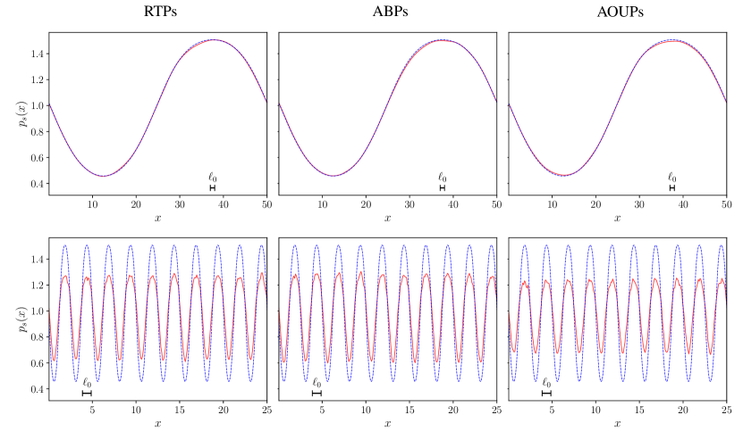
   Figure 2.2: Stationary distribution $p_{s}(x)$ of RTPs (left), ABPs (center) and AOUPs (right) in $2d$ with space-dependent $v_{0}({\bf r})=\bar{v}\exp[\sin(q_{n}x)]$, $q_{n}=2n\pi/L_{x}$, and finite translational diffusivity $D_{t}=0.3$. The blue dashed curve represents the theoretical prediction (2.102) obtained from the coarse-grained theory; the solid red curve is obtained from sampling the particle’s position in microscopic simulations. Top and bottom rows correspond to simulations with different wavevectors $q_{n}$ in $v_{0}(x)$. The bare persistence length $\ell_{0}\equiv\bar{v}\tau_{0}$ is shown for comparison at the bottom left of each panel. Parameters: $L_{x}=L_{y}=50$, $\bar{v}=1$. RTPs: $\alpha_{0}=1$. ABPs: $\Gamma_{0}=1$. AOUPs: $\omega_{0}=1$.

3 Interacting active particles from micro to macro

So far, we have considered the dynamics of non-interacting particles whose motility parameters depend on the position ${\bf r}$. We now turn to the case in which this motility regulation is the result of chemotactic or quorum-sensing interactions. As discussed in Sec. 1.4, such interactions are in general nonlocal so that the motility of a particle located at ${\bf r}$ admits a functional dependence on the density field:

$$\gamma({\bf r})\to\gamma({\bf r},[\rho])\;.$$ (3.1)

The dynamics of each particle is then coupled to the others’ via complex $N$-body interactions. Nevertheless, since the density $\rho(\mathbb{r})$ is a conserved field, its evolution is expected to occur on a large, diffusive timescale $T\sim L^{2}$. On time scales $\tau\ll\Delta t\ll L^{2}$, we thus expect the diffusive approximation to hold while $\rho(\mathbb{r})$ has not yet relaxed. Under this assumption of time-scale separation, which we refer to as a frozen-field approximation, the $N$-body problem is mapped back onto a system of $N$ independent particles, whose motility parameters depend only on position ${\bf r}$ (through the frozen field $\rho({\bf r})$). We can then use the result of the coarse-graining procedures detailed in Sec. 2.2 and 2.3 to predict the dynamics of $\rho$, which will occur on longer time scales.

In this. 3.1, we first test this idea at the single particle level by computing the particle mean-squared displacement (MSD) in a homogeneous system at density $\rho_{0}$. We then discuss how to generalize the Itō-Langevin dynamics describing the evolution of the density field to the case with interactions in Sec. 3.2. Then, starting from the resulting stochastic field theory, we derive in Sec. 3.3 the structure factor, the pair correlation function, and the intermediate scattering function for a system of active particles interacting via QS. Our analytical predictions are then tested against microscopic simulations of the interacting system.

3.1 Mean squared displacement

According to the diffusion-drift approximation, the motion of an active particle with motility regulation can be mapped to the passive Langevin dynamics (2.61), at mesoscopic scales $\ell_{p}\ll\Delta r\ll L$, $\tau\ll\Delta t\ll L^{2}$.

To test this idea, we focus on the case of QS interactions that regulate the self-propulsion speed, set $D_{t}=0$ and assume that the interactions can be considered as local, i.e. $v_{i}=v(\rho({\bf r}_{i}))$ for particle $i$. Integrating the microscopic dynamics, we obtain the trajectory of particle $i$ as:

$${\bf r}_{i}(t)=\int_{0}^{t}v({\bf r}_{i}(t^{\prime})){\bf u}_{i}(t^{\prime})\mathrm{d}t^{\prime}+{\bf r}_{i}(0)\;.$$ (3.2)

In $d$ space dimensions, the MSD is given by:

$$\langle\Delta r^{2}(t)\rangle = \langle|{\bf r}_{i}(t)-{\bf r}_{i}(0)|^{2}\rangle=\left\langle\left[\int_{0}^{t}v({\bf r}_{i}(t^{\prime})){\bf u}_{i}(t^{\prime})\mathrm{d}t^{\prime}\right]^{2}\right\rangle$$ (3.3)

$$= \int_{0}^{t}\mathrm{d}t^{\prime}\int_{0}^{t}\mathrm{d}t^{\prime\prime}\left\langle v({\bf r}_{i}(t^{\prime}))v({\bf r}_{i}(t^{\prime\prime})){\bf u}_{i}(t^{\prime})\cdot{\bf u}_{i}(t^{\prime\prime})\right\rangle\;.$$

Since the orientations decorrelate over a typical time $\tau$ as $\langle{\bf u}_{i}(t)\cdot{\bf u}_{i}(0)\rangle=e^{-t/\tau}$, we need to compute the correlations of $v(\mathbb{r})$ over spatial scales of the order of $\ell_{p}$. Assuming that the density field varies smoothly over space, we expand $v({\bf r}_{i}(t))-v({\bf r}_{i}(0))$ on scales of order $\ell_{p}$ as

$$v({\bf r}_{i}(t))=v({\bf r}_{i}(0))+\left.\frac{\partial v}{\partial\rho}\nabla_{{\bf r}}\rho\right|_{t=0,{\bf r}={\bf r}_{i}(0)}\cdot\left[{\bf r}_{i}(t)-{\bf r}_{i}(0)\right]=v({\bf r}_{i}(0))+\mathcal{O}\left(\frac{\ell_{p}}{L}\right)\;,$$ (3.4)

where we used the fact that $\nabla_{\bf r}\rho\sim\mathcal{O}(1/L)$. We then write:

$$\langle\Delta r^{2}(t)\rangle = v({\bf r}_{i}(0))^{2}\int_{0}^{t}\mathrm{d}t^{\prime}\int_{0}^{t}\mathrm{d}t^{\prime\prime}\left\langle{\bf u}_{i}(t^{\prime})\cdot{\bf u}_{i}(t^{\prime\prime})\right\rangle+\mathcal{O}\left(\frac{\ell_{p}}{L}\right)$$ (3.5)

$$= v({\bf r}_{i}(0))^{2}\int_{0}^{t}\mathrm{d}t^{\prime}\int_{0}^{t}\mathrm{d}t^{\prime\prime}e^{-|t^{\prime}-t^{\prime\prime}|/\tau}+\mathcal{O}\left(\frac{\ell_{p}}{L}\right)$$

$$= 2dt\left[\frac{v({\bf r}_{i}(0))^{2}\tau}{d}\right]+2v({\bf r}_{i}(0))^{2}\tau^{2}\left[e^{-t/\tau}-1\right]+\mathcal{O}\left(\frac{\ell_{p}}{L}\right)\;.$$

When the system has relaxed to a homogeneous state with density $\rho_{0}$, we can replace $\langle v({\bf r}_{i}(0))\rangle\simeq v(\rho_{0})$. Note that formula Eq. (3.5) is expected to hold for all times $t\ll L^{2}$. At the mesoscopic scale we also have $t\gg\tau$ and the second contribution in Eq. (3.5) is subleading: we then obtained the MSD in terms of the mesoscopic diffusivity

$$\mathcal{D}(\rho_{0})=\frac{1}{2dt}\>\lim_{\begin{subarray}{c}t/\tau\to\infty\\ t/L^{2}\to 0\end{subarray}}\langle\Delta r^{2}(t)\rangle=\frac{v(\rho_{0})^{2}\tau}{d}\;,$$ (3.6)

corresponding to the result (2.60) obtained from the diffusion-drift approximation. If the homogeneous profile is stable we expect this equality to hold also at steady-state, hence also for diffusive times $t\sim\mathcal{O}(L^{2})$. This is indeed observed in simulations, as reported in Fig. (3.1).

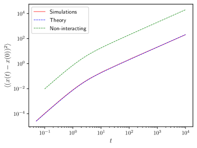
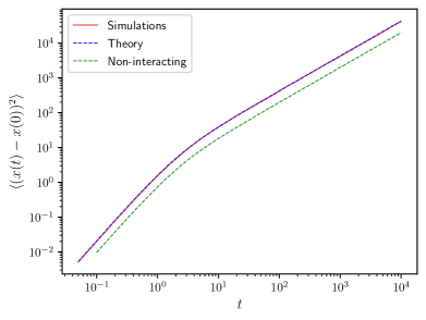
Figure 3.1: Mean-square displacement for a homogeneous system of RTPs in $1d$ interacting via QS through $v(\rho)=v_{0}\exp\left\{\kappa\tanh\left[(\rho-\rho_{m})/{\varphi}\right]\right\}$. The panels show comparisons between numerical measurements (solid red lines) and diffusion-drift theory (3.5) (dashed blue lines). The non-interacting prediction for the MSD ($v\equiv v_{0}$) is also reported for comparison (dashed green lines). (Left) motility enhancement, $\kappa=3$. (Right) Motility inhibition, $\kappa=-0.50$. Parameters of the simulation: $\rho_{0}=30,\rho_{m}=50,\varphi=20,\alpha_{0}=1,v_{0}=1$. Size of the simulation domain $L_{x}=100$.

3.2 From mesoscopic to macroscopic description

Thanks to the frozen-field approximation, we can thus approximation the dynamics of our active particles on mesoscopic times as:

$$\dot{{\bf r}}_{i}=\mathbf{V}({\bf r}_{i},[\rho])+\nabla_{{\bf r}_{i}}\mathcal{D}({\bf r}_{i},[\rho])+\sqrt{2\mathcal{D}({\bf r}_{i},[\rho])}\boldsymbol{\xi}_{i}(t)\;,$$ (3.7)

where the $\{\boldsymbol{\xi}_{i}(t)\}$ are delta-correlated, centered Gaussian white noises. Note that, at this stage, we have re-inserted the density dependences, since we are now looking at the system at a scale which is way larger than the persistence length. Restoring this density-dependence in $\mathcal{D}$, the gradient $\nabla_{{\bf r}_{i}}$ in principle acts both on the first variable and on the field $[\rho]$, the latter because $\rho$ is affected by a change in $\mathbf{r}_{i}$:

$$\nabla_{\mathbf{r}_{i}}\mathcal{D}(\mathbf{r}_{i},[\rho])=\nabla_{1}\mathcal{D}(\mathbf{r}_{i},[\rho])+\int\mathrm{d}^{d}{\bf r}^{\prime}\frac{\delta\mathcal{D}({\bf r}_{i})}{\delta\rho({\bf r}^{\prime})}\nabla_{{\bf r}_{i}}\rho({\bf r}^{\prime})\;.$$ (3.8)

where $\nabla_{1}$ denotes the derivative with respect to the first variable. However, it can be shown that the second term of Eq. (3.8) vanishes in many cases of interest [37]. In particular, this occurs whenever $\mathcal{D}$ is a function of an effective density $\tilde{\rho}$, obtained by convolution of $\rho({\bf r})$ with a symmetric kernel $K({\bf r})$:

$$\mathcal{D}({\bf r},[\rho])=\mathcal{D}(\tilde{\rho}({\bf r}))\;,\qquad\tilde{\rho}({\bf r})\equiv(K\circledast\rho)({\bf r})=\int\mathrm{d}^{d}{\bf r}^{\prime}\>K({\bf r}-{\bf r}^{\prime})\rho({\bf r}^{\prime})\;.$$ (3.9)

To see this, we use the definition of $\rho({\bf r}^{\prime})$:

$$\nabla_{{\bf r}_{i}}\rho({\bf r}^{\prime})=\nabla_{{\bf r}_{i}}\sum_{j}\delta({\bf r}^{\prime}-{\bf r}_{j})=\nabla_{{\bf r}_{i}}\delta({\bf r}^{\prime}-{\bf r}_{i})=-\nabla_{{\bf r}^{\prime}}\delta({\bf r}^{\prime}-{\bf r}_{i})\;$$ (3.10)

and re-write Eq. (3.8) as:

$$\nabla_{{\bf r}_{i}}\mathcal{D} = \nabla_{1}\mathcal{D}-\int\mathrm{d}^{d}{\bf r}^{\prime}\frac{\delta\mathcal{D}({\bf r}_{i})}{\delta\rho({\bf r}^{\prime})}\nabla_{{\bf r}^{\prime}}\delta({\bf r}^{\prime}-{\bf r}_{i})=\nabla_{1}\mathcal{D}+\int\mathrm{d}^{d}{\bf r}^{\prime}\left[\nabla_{{\bf r}^{\prime}}\frac{\delta\mathcal{D}({\bf r}_{i})}{\delta\rho({\bf r}^{\prime})}\right]\delta({\bf r}^{\prime}-{\bf r}_{i})$$ (3.11)

$$= \nabla_{1}\mathcal{D}+\left[\nabla_{{\bf r}^{\prime}}\frac{\delta\mathcal{D}({\bf r}_{i})}{\delta\rho({\bf r}^{\prime})}\right]_{{\bf r}^{\prime}={\bf r}_{i}}\;.$$

Applying the chain rule for functional derivatives:

$$\nabla_{{\bf r}^{\prime}}\frac{\delta\mathcal{D}({\bf r}_{i})}{\delta\rho({\bf r}^{\prime})} = \nabla_{{\bf r}^{\prime}}\int\mathrm{d}{\bf r}^{\prime\prime}\frac{\delta\mathcal{D}({\bf r}_{i})}{\delta\tilde{\rho}({\bf r}^{\prime\prime})}\frac{\delta\tilde{\rho}({\bf r}^{\prime\prime})}{\delta\rho({\bf r}^{\prime})}=\int\mathrm{d}{\bf r}^{\prime\prime}\frac{\partial\mathcal{D}}{\partial\tilde{\rho}}\delta({\bf r}_{i}-{\bf r}^{\prime\prime})\>\nabla_{{\bf r}^{\prime}}\frac{\delta\tilde{\rho}({\bf r}^{\prime\prime})}{\delta\rho({\bf r}^{\prime})}\;,$$ (3.12)

where in the last passage we have expanded the functional derivative $\delta\mathcal{D}({\bf r}_{i})/\delta\tilde{\rho}({\bf r}^{\prime\prime})$. Integrating over ${\bf r}^{\prime\prime}$ then gives:

$$\nabla_{{\bf r}^{\prime}}\frac{\delta\mathcal{D}({\bf r}_{i})}{\delta\rho({\bf r}^{\prime})} = \frac{\partial\mathcal{D}}{\partial\tilde{\rho}}\nabla_{{\bf r}^{\prime}}\frac{\delta\tilde{\rho}({\bf r}_{i})}{\delta\rho({\bf r}^{\prime})}=\frac{\partial\mathcal{D}}{\partial\tilde{\rho}}\nabla_{{\bf r}^{\prime}}K({\bf r}_{i}-{\bf r}^{\prime})\;.$$ (3.13)

Finally, since $K({\bf r})$ is symmetric around the origin, we conclude:

$$\left[\nabla_{{\bf r}^{\prime}}\frac{\delta\mathcal{D}({\bf r}_{i})}{\delta\rho({\bf r}^{\prime})}\right]_{{\bf r}^{\prime}={\bf r}_{i}}=-\frac{\partial\mathcal{D}}{\partial\tilde{\rho}}\nabla_{\bf r}K(0)=0\;.$$ (3.14)

We note that such a symmetric $K$ is expected in the case where the interactions are mediated by a diffusive field, as suggested by Eq. (1.21). In the following, we thus neglect this contribution to the Itô drift.

Starting from the mesoscopic Langevin description of Eq. (3.7), one can thus reproduce the derivation of Sec. 2.4 to obtain the fluctuating hydrodynamics of $\rho$:

$$\partial_{t}\rho=-\nabla_{\mathbf{r}}\cdot\biggl{\{}\mathbf{V}(\mathbf{r},[\rho])\rho-\mathcal{D}(\mathbf{r},[\rho])\nabla_{\mathbf{r}}\rho+\sqrt{2\mathcal{D}(\mathbf{r},[\rho])\rho}\>\>\mathbf{\Lambda}(\mathbf{r},t)\biggr{\}}\;,$$ (3.15)

where we remind that the expressions of $\mathbf{V}$ and $\mathcal{D}$ are given by Eq. (2.60) for RTP-ABPs and Eq. (2.89) for AOUPs.

3.3 Correlation functions in interacting particle systems

The stochastic hydrodynamics (3.15) can be used determine correlation functions at the steady state for our non-equilibrium, interacting systems. We devote this section to the derivation of the static structure factor $S({\bf q})$, spatial correlation function $G({\bf r})$ and intermediate scattering function $F({\bf q},t)$ for an active system with motility regulation. The method presented here extends [68] to an out-of-equilibrium setup. Our analytical prediction are tested against numerical simulations in Sec. 3.3.3.

As a microscopic model, we take the case of RTPs interacting via QS with:

$$\begin{cases}&v({\bf r},[\rho])=v(\tilde{\rho}({\bf r}))\\ &\alpha({\bf r},[\rho])=\alpha(\tilde{\rho}({\bf r}))\\ \end{cases}\quad\qquad\tilde{\rho}({\bf r})=(K\circledast\rho)({\bf r})=\int d^{d}{\bf r}^{\prime}\;K({\bf r}-{\bf r}^{\prime})\rho({\bf r}^{\prime})\;,$$ (3.16)

where $\tilde{\rho}$ represents an effective density at point ${\bf r}$, obtained by weighing the contribution of each particle by a kernel $K({\bf r})$. We take $K({\bf r})$ to be normalized and isotropic.

We then consider the corresponding stochastic field theory (3.15) and study the dynamics of density fluctuations $\delta\rho=\rho-\rho_{0}$ around a stable homogeneous profile $\rho_{0}$ at steady state. To do so, we first derive the linearized hydrodynamics of our system. Expanding the diffusive and drift terms in Eq. (3.15) we obtain:

$$\mathcal{D}\nabla_{\bf r}\delta\rho = \frac{v^{2}(\boldsymbol{r},[\rho])}{d\alpha(\boldsymbol{r},[\rho])}\nabla_{\bf r}\delta\rho=\frac{v^{2}(\rho_{0})}{d\alpha(\rho_{0})}\nabla_{\bf r}\delta\rho+\mathcal{O}(\delta\rho^{2})\equiv\mathcal{D}_{0}\nabla_{\bf r}\delta\rho+\mathcal{O}(\delta\rho^{2})\;,$$ (3.17)

$$\boldsymbol{V}\rho = -\frac{v(\boldsymbol{r},[\rho])\nabla_{\bf r}v(\boldsymbol{r},[\rho])}{d\alpha(\boldsymbol{r},[\rho])}(\rho_{0}+\delta\rho)=-\frac{vv^{\prime}(\tilde{\rho}({\bf r}))}{d\alpha(\tilde{\rho}({\bf r}))}(\rho_{0}+\delta\rho)\nabla_{\bf r}\delta\tilde{\rho}({\bf r})$$ (3.18)

$$= -\mathcal{D}_{0}\rho_{0}\frac{d\log v_{0}}{d\tilde{\rho}}\nabla_{\bf r}(K\circledast\delta\rho)({\bf r})+\mathcal{O}(\delta\rho^{2})\;.$$

To treat the conserved noise term $\nabla_{{\bf r}}\cdot\left[\sqrt{2\mathcal{D}({\bf r},[\rho])}\boldsymbol{\Lambda}({\bf r},t)\right]$, we expand:

$$2\mathcal{D}(\tilde{\rho}({\bf r}))\rho({\bf r})=2\mathcal{D}_{0}\rho_{0}\left[1+\frac{1}{\mathcal{D}_{0}}\left.\frac{d\mathcal{D}_{0}}{d\tilde{\rho}}\right|_{\tilde{\rho}=\rho_{0}}\left(K\circledast\frac{\delta\rho}{\rho_{0}}\right)({\bf r})+\frac{\delta\rho}{\rho_{0}}\right]+\mathcal{O}\left(\delta\rho^{2}\right)\;.$$ (3.19)

When the homogeneous profile $\rho_{0}$ is stable, we expect density fluctuations $\delta\rho$ to scale as $\sqrt{\rho_{0}}$. At large densities, we can thus retain only the leading-order contribution to the noise, which becomes additive and delta-correlated:

$$\nabla_{{\bf r}}\cdot\left[\sqrt{2\mathcal{D}({\bf r},[\rho])}\boldsymbol{\Lambda}({\bf r},t)\right]\approx\nabla_{\bf r}\cdot\left[\sqrt{2\mathcal{D}_{0}\rho_{0}}\boldsymbol{\Lambda}({\bf r},t)\right]\;.$$ (3.20)

All in all, we obtain the linear dynamics of $\delta\rho$ as:

$$\partial_{t}\delta\rho=\mathcal{D}_{0}\nabla_{\bf r}^{2}\left[\frac{d\log v_{0}}{d\tilde{\rho}}\rho_{0}\;(K\circledast\delta\rho)+\delta\rho\right]+\nabla_{\bf r}\cdot\left[\sqrt{2\mathcal{D}_{0}\rho_{0}}\boldsymbol{\Lambda}({\bf r},t)\right]\;.$$ (3.21)

Next, we write Eq. (3.21) in Fourier space. In a finite volume $L^{d}$, we adopt the following convention for the Fourier transform:

$$f({\bf r})=\frac{1}{L^{d}}\sum_{n=-\infty}^{+\infty}e^{i{\bf q}_{n}\cdot{\bf r}}\hat{f}_{n}\>,\qquad\hat{f}_{n}=\int_{L^{d}}e^{-i{\bf q}_{n}\cdot{\bf r}}f({\bf r})\>d^{d}{\bf r}\>,\qquad{\bf q}_{n}=\frac{2\pi}{L}(n_{1},n_{2},\dots,n_{d})\;.$$ (3.22)

The dynamics in Fourier space then reads:

$$\partial_{t}\delta\hat{\rho}_{n}=-q_{n}^{2}\mathcal{D}_{0}\left(\frac{d\log v_{0}}{d\tilde{\rho}}\rho_{0}\;\hat{K}_{n}+1\right)\delta\hat{\rho}_{n}-\sqrt{2\mathcal{D}_{0}\rho_{0}}\;i{\bf q}_{n}\cdot\hat{\mathbf{\Lambda}}_{n}\;,$$ (3.23)

where the Gaussian white noise in Fourier space satisfies: $\langle\hat{\mathbf{\Lambda}}_{n}(t)\hat{\mathbf{\Lambda}}_{m}(t^{\prime})\rangle=L^{d}\delta_{n,-m}\delta(t-t^{\prime})$. We note that Eq. (3.23) leads to an exponential growth of $\delta\hat{\rho}_{n}$ when:

$$-\mathcal{D}_{0}\left(\rho_{0}\frac{d\log v_{0}}{d\tilde{\rho}_{0}}\hat{K}_{n}+1\right)q_{n}^{2}>0\;\;.$$ (3.24)

Otherwise, the homogeneous configuration is (linearly) stable and density fluctuations are damped. For hydrodynamic modes where ${\bf q}_{n}\to 0$, $K_{n}\to 1$ and the homogeneous profile is linearly unstable when:

$$\frac{d\log v(\tilde{\rho})}{d\tilde{\rho}}<-\frac{1}{\rho_{0}}\;,$$ (3.25)

corresponding to the condition for a spinodal stability in QS-MIPS [9]. In the following we choose parameters such that (3.25) is far from being satisfied, so that $\delta\hat{\rho}_{n}$ relaxes and its dynamics is well described by Eq. (3.23). As a final remark, note that $\delta\hat{\rho}_{n=0}(t)=0$ at any time $t$, due to mass conservation:

$$\delta\hat{\rho}_{0}(t)=\hat{f}_{n}=\int_{L^{d}}(\rho({\bf r},t)-\rho_{0})=0\;.$$ (3.26)

3.3.1 Statics: Structure factor and pair correlation function

At steady state, the static structure factor is defined as:

$$S({\bf q}_{n})\equiv\frac{1}{N}\langle\delta\hat{\rho}_{n}\delta\hat{\rho}_{-n}\rangle\;.$$ (3.27)

Using the Itô chain rule together with the dynamics (3.23) we can compute:

$$\partial_{t}\langle\delta\hat{\rho}_{n}\delta\hat{\rho}_{m}\rangle =\langle(\partial_{t}\delta\hat{\rho}_{n})\delta\hat{\rho}_{m}\rangle+\langle\delta\hat{\rho}_{n}(\partial_{t}\delta\hat{\rho}_{m})\rangle-2{\bf q}_{n}\cdot{\bf q}_{m}\mathcal{D}_{0}\rho_{0}L^{d}\delta_{n,-m}$$ (3.28)

$$\begin{split}=-\mathcal{D}_{0}\left[\left(\rho_{0}\frac{d\log v_{0}}{d\tilde{\rho}_{0}}\hat{K}_{n}+1\right)q_{n}^{2}+\left(\rho_{0}\frac{d\log v_{0}}{d\tilde{\rho}}\hat{K}_{m}+1\right)q_{m}^{2}\right]\langle\delta\hat{\rho}_{n}\delta\hat{\rho}_{m}\rangle\\ -2{\bf q}_{n}\cdot{\bf q}_{m}\mathcal{D}_{0}\rho_{0}L^{d}\delta_{n,-m}\;.\end{split}$$

When the spinodal instability condition is violated (3.25), the linear dynamics for $\langle\delta\hat{\rho}_{n}\delta\hat{\rho}_{m}\rangle$ admits a stationary solution. At steady state, Eq. (3.28) leads to:

$$\langle\delta\hat{\rho}_{n}\delta\hat{\rho}_{m}\rangle=\begin{cases}&\dfrac{-2{\bf q}_{n}\cdot{\bf q}_{m}\rho_{0}L^{d}}{\left(\rho_{0}\dfrac{d\log v_{0}}{d\tilde{\rho}}\hat{K}_{n}+1\right)q_{n}^{2}+\left(\rho_{0}\dfrac{d\log v_{0}}{d\tilde{\rho}}\hat{K}_{m}+1\right)q_{m}^{2}}\delta_{n,-m}\qquad n,m\neq 0\\[28.45274pt] &0\hskip 256.0748ptn=m=0\end{cases}$$ (3.29)

The only non-zero contributions to the correlations thus come from ${\bf q}_{n}=-{\bf q}_{m}$:

$$\langle\delta\hat{\rho}_{n}\delta\hat{\rho}_{-n}\rangle=\frac{\rho_{0}L^{d}}{1+\rho_{0}\dfrac{d\log v_{0}}{d\tilde{\rho}}\hat{K}_{n}}(1-\delta_{n,0})$$ (3.30)

We can finally write the expression of the structure factor:

$$S({\bf q}_{n})=\frac{\langle\delta\hat{\rho}_{n}\delta\hat{\rho}_{-n}\rangle}{N}=\frac{1-\delta_{n,0}}{1+\rho_{0}\dfrac{d\log v_{0}}{d\tilde{\rho}}\hat{K}_{n}}\;.$$ (3.31)

From the knowledge of $\langle\delta\hat{\rho}_{n}\delta\hat{\rho}_{m}\rangle$ at steady state we can then compute the spatial correlation function:

$$G({\bf r},{\bf r}^{\prime})\equiv\langle\delta\rho({\bf r})\;\delta\rho({\bf r}^{\prime})\rangle\;.$$ (3.32)

By decomposing $\delta\rho({\bf r})$ into Fourier modes, we find:

$$G({\bf r},{\bf r}^{\prime}) = \frac{1}{L^{2d}}\sum_{n,m}e^{i{\bf q}_{n}\cdot{\bf r}}e^{i{\bf q}_{m}\cdot{\bf r}^{\prime}}\langle\delta\hat{\rho}_{n}\delta\hat{\rho}_{m}\rangle=\frac{1}{L^{2d}}\sum_{n}e^{i{\bf q}_{n}\cdot({\bf r}-{\bf r}^{\prime})}\rho_{0}L^{d}S({\bf q}_{n})$$ (3.33)

$$= \rho_{0}\left[\frac{1}{L^{d}}\sum_{n}e^{i{\bf q}_{n}\cdot({\bf r}-{\bf r}^{\prime})}S({\bf q}_{n})\right]\;.$$

Since $S({\bf q}_{n})\to 1$ for ${\bf q}_{n}\to\infty$, it is convenient to shift it by a constant $-1$ to perform the Fourier transform. Eventually, this gives:

$$\frac{G({\bf r},{\bf r}^{\prime})}{\rho_{0}} = \frac{1}{L^{d}}\sum_{n}e^{i{\bf q}_{n}\cdot({\bf r}-{\bf r}^{\prime})}\left[S({\bf q}_{n})-1\right]+\delta({\bf r}-{\bf r}^{\prime})\;.$$ (3.34)

For ${\bf r}\neq{\bf r}^{\prime}$, the inverse Fourier transform of $[S({\bf q})-1]$ thus corresponds to the spatial correlation function $G({\bf r},{\bf r}^{\prime})/\rho_{0}$.

3.3.2 Dynamics: Intermediate scattering function

Finally, we derive the expression of the intermediate scattering function:

$$F({\bf q},t)=\lim_{\tau\to\infty}\frac{1}{N}\langle\delta\hat{\rho}_{{\bf q}}(\tau+t)\;\delta\hat{\rho}_{-{\bf q}}(\tau)\rangle\;.$$ (3.35)

By definition, the intermediate scattering function at $t=0$ coincides with the static structure factor $S({\bf q})$. Starting from the linearized dynamics of $\delta\rho$ in Fourier space (3.23), we compute:

$$\partial_{t}F({\bf q}_{n},t) = \partial_{t}\frac{\langle\delta\hat{\rho}_{n}(\tau+t)\;\delta\hat{\rho}_{-n}(\tau)\rangle}{N}=\frac{\langle\partial_{t}\delta\hat{\rho}_{n}(\tau+t)\;\delta\hat{\rho}_{-n}(\tau)\rangle}{N}$$ (3.36)

$$= -q_{n}^{2}\mathcal{D}_{0}\left(1+\frac{d\log v_{0}}{d\tilde{\rho}}\rho_{0}\;\hat{K}_{n}\right)F({\bf q}_{n},t)\;.$$

Solving for $F({\bf q}_{n})$ with the initial condition $F({\bf q}_{n},t=0)=S({\bf q}_{n})$, we obtain:

$$F({\bf q}_{n},t)=S({\bf q}_{n})\;\exp\left[-q_{n}^{2}\mathcal{D}_{0}\left(1+\frac{d\log v_{0}}{d\tilde{\rho}}\rho_{0}\;\hat{K}_{n}\right)t\right]\;.$$ (3.37)

Finally, in the limit of local interactions $K({\bf r})\equiv\delta({\bf r})$, the intermediate scattering function decays as:

$$F({\bf q},t)=S({\bf q})\;e^{-q^{2}\mathcal{D}_{\text{eff}}\;t}\;,\qquad\mathcal{D}_{\text{eff}}\equiv\mathcal{D}_{0}\left(1+\frac{d\log v_{0}}{d\tilde{\rho}}\rho_{0}\;\right)\;.$$ (3.38)

It can be instructive to compare this result with $F({\bf q},t)$ in an ideal gas. In the latter, it is known [69] that the intermediate scattering function decays exponentially in time with a rate $\mathcal{D}_{0}q^{2}$, where $\mathcal{D}_{0}$ is the diffusivity of the gas. This scaling is found also in the active case, as shown in Eq. (3.38); however, the value of the effective diffusivity $\mathcal{D}_{\text{eff}}$ in the active gas is renormalized by QS interactions.

3.3.3 Simulations

To test the predictions of our field theory (2.100), we perform particle-based simulations with QS-RTPs in $1d$ moving according to the dynamics (1.2). We consider a self-propulsion speed regulated as:

$$v(\tilde{\rho}) = v_{0}\exp\left[\kappa\tanh\left(\frac{\tilde{\rho}-\rho_{m}}{\varphi}\right)\right]\;,$$ (3.39)

$$\tilde{\rho}(x) = (K\circledast\rho)(x)\;,\qquad K(x)=\frac{1}{Z}\exp\left(-\frac{r_{0}^{2}}{r_{0}^{2}-x^{2}}\right)\theta(r_{0}-|x|)\;,$$ (3.40)

where $\circledast$ denotes the convolution product, and $Z$ is a normalization factor for the bell-shaped convolution kernel $K$. The tumbling rate $\alpha_{0}$ is kept constant, and the QS-interaction radius $r_{0}=1$.

We simulate our system for values of the parameters where the steady-state configuration is homogeneous and measure both the structure factor $S(q)$ and the correlation function $G(r)$. As shown in Fig. 3.2, the agreement between theory and simulations is remarkable at sufficiently large densities, with no fitting parameter being used. We note that, at smaller densities, discrepancies between our final predictions and numerical simulations are both expected and observed, due to the failure of the additive-noise approximation, Eq. (3.20) (See Fig. 3.3).

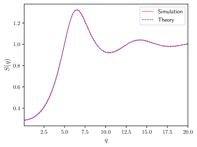
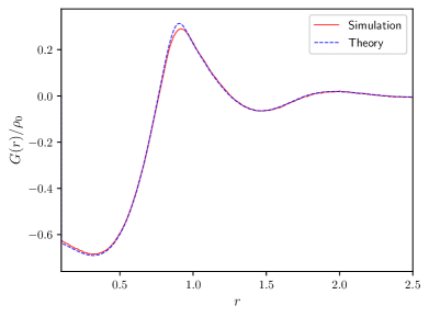
Figure 3.2: Structure factor $S(q)$ (left) and spatial correlation function $G(r)$ (right) for a homogeneous gas of RTPs interacting via QS according to Eq (3.39): comparison between numerical measurements (solid line) and theoretical predictions from Eqs. (3.31), (3.34) (dashed blue line). Parameters of the simulation: $\rho_{0}=50,\rho_{m}=50,\varphi=20,\alpha_{0}=2,v_{0}=1,\kappa=1$. Size of the simulation domain $L_{x}=1000$.

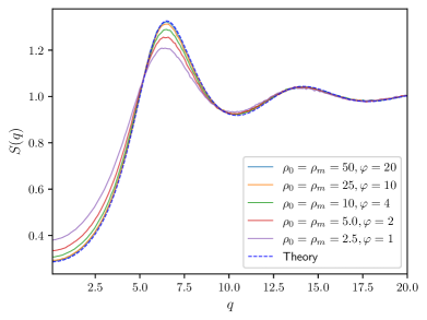
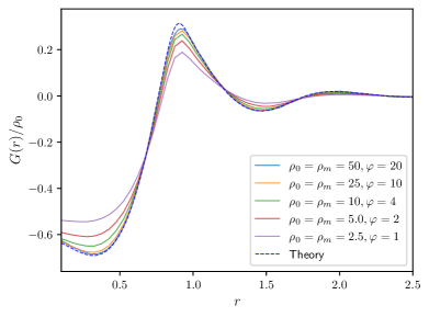
Figure 3.3: Structure factor $S(q)$ (left) and spatial correlation function $G(r)$ (right) for a homogeneous gas of RTPs interacting via QS according to Eq (3.39) for different values of the density $\rho_{0}$: comparison between numerical measurements (solid lines) and theoretical predictions from Eqs. (3.31), (3.34) (dashed blue line). Parameters of the simulation: $\rho_{0}=\rho_{m},\varphi=2/5\leavevmode\nobreak\ \rho_{m},\alpha_{0}=2,v_{0}=1,\kappa=1$. Size of the simulation domain $L_{x}=1000$.

We then turn to the measurement of the intermediate scattering function $F(q,t)$. We consider a system with motility enhancement ($\kappa>0$) and fix the density $\rho_{0}$. For a range of Fourier modes, we measure the decay time $\tau(q)$ of the corresponding $F(q,t)$ from simulations. We then fit the curve $\tau(q)$ and determine the value of the effective diffusivity $\mathcal{D}_{\text{eff}}$, defined as in Eq. (3.38). By comparing the measured effective diffusivity with its theoretical value, we are able to test our analytical predictions for $F(q,t)$. For an average density of $\rho_{0}=30$, the theoretical value of $\mathcal{D}_{\text{eff}}=0.614$ is in good agreement with the result obtained from the fit: $\mathcal{D}_{\text{eff}}^{\>\text{fit}}=0.626\pm 0.001$. In the left panel of Figure 3.4, we report three examples for different modes of the exponential decay of $F(q,t)$. In the right panel, we plot $\tau(q)$ as a function of the inverse wavelength $q$, comparing the results from our simulations with the analytical predictions.

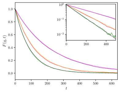
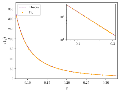
Figure 3.4: Measurements of the intermediate scattering function for a homogeneous gas of RTPs interacting via QS according to Eq (3.39) in $1d$. (Left): intermediate scattering function $F(q,t)$ for three different Fourier modes ($q=0.085$ in magenta, $q=0.113$ in orange, $q=0.132$ in green). The solid curves represent the theoretical predictions from Eq. (3.38), while the dashed lines correspond to $F(q,t)$ measured from simulations. The same curves are represented in semi-log scale in the inset, to highlight the exponential behaviour. (Right): Decay time $\tau(q)$ of $F(q,t)$ as a function of the wave-vector $q$. Data-points are obtained by measuring $\tau$ from the decay of $F(q,t)$ at a given $q$; the errorbars are so small that they are not visible ($\sim 10^{-3}$). The fitted curve (orange) is then compared with our theoretical prediction (purple) from Eq. (3.38). The inset shows the same curves in log-log scale, to highlight the power-law behaviour. Parameters of the simulation: $\rho_{0}=30,\rho_{m}=50,\varphi=20,\alpha_{0}=1,v_{0}=1,\kappa=0.5$. Size of the simulation domain $L_{x}=2000$.

4 Active mixtures

In this Section, we show how the methods described in the previous sections can be generalized to active mixtures. Multi-component active systems have drawn increasing attention in recent years [70, 71, 21, 22, 72, 24], due to the rich phenomenology they exhibit both at the static and dynamical level: from the demixing of two E. Coli strains [12] to run-and-chase dynamics in bacterial mixtures [73, 74] and emergent chiral phases in two species of aligning particles [23, 75]. To understand–and possibly control–the wealth of phenomena that emerge in these systems we thus need to bridge between microscopic and macroscopic dynamics of active mixtures. Here we consider a system of $N$ particles belonging to $S$ different species; we label each species with an index $\mu\in\{1,\dots,S\}$, and assume that there are a total of $N_{\mu}$ particle of type $\mu$. Each particle will thus be identified by a pair of indices $(i,\mu)$, with $i\in\{1,\dots,N_{\mu}\}$. Finally, we denote by $\rho_{\mu}$ the density field associated with species $\mu$, defined as:

$$\rho_{\mu}({\bf r},t)=\sum_{i=1}^{N_{\mu}}\delta({\bf r}-{\bf r}_{i,\mu}(t))\;.$$ (4.1)

Each $(i,\mu)$-particle undergoes motility regulation through QS via:

$$\gamma_{\mu}=\gamma_{0\mu}({\bf r}_{i,\mu},[\{\rho_{\nu}\}])\;,$$ (4.2)

where $\gamma_{\mu}$ stands for any motility parameter (persistence time, self-propulsion speed…). As regards to chemotaxis, we consider the general case where the bias on particle $(i,\mu)$ is generated by the gradients of $n$ different chemical fields $\{c_{h}({\bf r})\}$:

$$\gamma_{\mu}=\gamma_{\mu}({\bf r}_{i,\mu},\{\nabla_{\bf r}c_{h}({\bf r})\})\;.$$ (4.3)

For tactic interactions, the chemical fields are taken to be functionals of the density fields: $c_{h}({\bf r},\{[\rho_{\nu}]\})$. All in all, we express the effect of QS and chemotaxis on motility as:

$$\gamma_{\mu}({\bf r}_{i,\mu},\{[\rho_{\nu}]\})=\gamma_{0\mu}({\bf r}_{i,\mu},\{[\rho_{\nu}]\})+{\bf u}_{i,\mu}\cdot\sum_{h=1}^{n}\gamma_{1\mu}^{h}\nabla_{{\bf r}_{i,\mu}}c_{h}({\bf r}_{i,\mu},\{[\rho_{\nu}]\})\;.$$ (4.4)

As in Sec. 3, we assume a separation of time scales between the fast microscopic degrees of freedom and the slowly diffusing density fields. Hence, we map the $N$-body microscopic dynamics into a non-interacting problem through the frozen-field approximation, thanks to which the motility parameters become position-dependent functions. We are thus able to write down the master equation for the probability $\mathcal{P}_{\mu}({\bf r},{\bf u})$ of finding a particle of type $\mu$ in position ${\bf r}$ with orientation ${\bf u}$.

For a mixture of RTPs and ABPs, the $S$-species master equation generalizes the single-species one, Eq. (2.44), as:

$$\partial_{t}\mathcal{P}_{\mu}(\mathbb{r},\mathbb{u})=-\nabla_{\mathbb{r}}\cdot\left[v_{\mu}\mathbb{u}\mathcal{P}_{\mu}-D_{t\mu}\nabla_{\mathbb{r}}\mathcal{P}_{\mu}\right]-\alpha_{\mu}\mathcal{P}_{\mu}+\frac{1}{\Omega}\int\alpha_{\mu}\mathcal{P}_{\mu}\mathrm{d}{\bf u}+\Delta_{\mathbb{u}}\Gamma_{\mu}\mathcal{P}_{\mu}\;,$$ (4.5)

where the motility parameters are given by:

$$v_{\mu} = v_{0\mu}({\bf r})-{\bf u}\cdot\sum_{h=1}^{n}v_{1\mu}^{h}\>\nabla_{\bf r}c_{h}({\bf r})$$ (4.6)

$$\alpha_{\mu} = \alpha_{0\mu}({\bf r})+{\bf u}\cdot\sum_{h=1}^{n}\alpha_{1\mu}^{h}\>\nabla_{\bf r}c_{h}({\bf r})$$ (4.7)

$$\Gamma_{\mu} = \Gamma_{0\mu}({\bf r})+{\bf u}\cdot\sum_{h=1}^{n}\Gamma_{1\mu}^{h}\>\nabla_{\bf r}c_{h}({\bf r})\;.$$ (4.8)

Similarly, for a mixture of AOUPs, the single-species master equation (2.65) is generalized to:

$$\partial_{t}\mathcal{P}_{\mu}(\mathbb{r},\mathbb{e}) = -\nabla_{\mathbb{r}}\cdot\left[v_{\mu}\mathbb{e}\mathcal{P}_{\mu}-D_{t\mu}\nabla_{\mathbb{r}}\mathcal{P}_{\mu}\right]-\nabla_{\mathbb{e}}\cdot\left[-\tau_{\mu}^{-1}\mathbb{e}\mathcal{P}_{\mu}-\frac{1}{d}\nabla_{\mathbb{e}}(\tau_{\mu}^{-1}\mathcal{P}_{\mu})\right]\;,$$ (4.9)

with:

$$v_{\mu} = v_{0\mu}({\bf r})-{\bf e}\cdot\sum_{h=1}^{n}v_{1\mu}^{h}\>\nabla_{\bf r}c_{h}({\bf r})$$ (4.10)

$$\tau_{\mu}^{-1} = \omega_{0\mu}({\bf r})+{\bf e}\cdot\sum_{h=1}^{n}\omega_{1\mu}^{h}\>\nabla_{\bf r}c_{h}({\bf r})\;.$$ (4.11)

Starting from the microscopic dynamics (4.5), (4.9), one then follows the same steps as in the single-species case presented in Sec. 2.2 to obtain an effective Langevin description at the mesoscopic scale. For the sake of completeness, we report the full computation in Appendix D. Under the diffusion-drift approximation, the large-scale dynamics of particle $i$ of type $\mu$ eventually follows an Itô-Langevin equation:

$$\dot{{\bf r}}_{i,\mu}=\mathbf{V}_{\mu}({\bf r}_{i,\mu},[\{\rho_{\nu}\}])+\nabla_{{\bf r}_{i,\mu}}\mathcal{D}_{\mu}({\bf r}_{i,\mu},[\{\rho_{\nu}\}])+\sqrt{2\mathcal{D}_{\mu}({\bf r}_{i,\mu},[\{\rho_{\nu}\}])}\boldsymbol{\xi}_{i,\mu}(t)$$ (4.12)

where the $\{\boldsymbol{\xi}_{i,\mu}(t)\}$ are delta-correlated, centred Gaussian white noise terms, and:

$$\text{ABP-RTP}: \begin{cases}&\mathbf{V}_{\mu}=-\dfrac{v_{0\mu}\nabla v_{0\mu}}{d\left[\alpha_{0\mu}+(d-1)\Gamma_{0\mu}\right]}-\dfrac{1}{d}\sum_{h=1}^{n}\left[v_{1\mu}^{h}+v_{0\mu}\dfrac{\alpha_{1\mu}^{h}+(d-1)\Gamma_{1\mu}^{h}}{\alpha_{0\mu}+(d-1)\Gamma_{0\mu}}\right]\nabla_{{\bf r}}c_{h}\\[17.07182pt] &\mathcal{D}_{\mu}=\dfrac{v_{0\mu}^{2}}{d\left[\alpha_{0\mu}+(d-1)\Gamma_{0\mu}\right]}+D_{t\mu}\ .\end{cases}$$ (4.13)

$$\text{AOUP}: \begin{cases}&\mathbf{V}_{\mu}=-\dfrac{v_{0\mu}\nabla v_{0\mu}}{d\omega_{0\mu}}-\dfrac{1}{d}\sum_{h=1}^{n}\left[v_{1\mu}^{h}+v_{0\mu}\dfrac{\omega_{1\mu}^{h}}{\omega_{0\mu}}\right]\nabla_{{\bf r}}c_{h}\\[17.07182pt] &\mathcal{D}_{\mu}=\dfrac{v_{0\mu}^{2}}{d\omega_{0\mu}}+D_{t\mu}\ .\end{cases}$$ (4.14)

4.1 Coupled fluctuating hydrodynamics for active mixtures

Starting from the stochastic dynamics (4.12) we now derive the time-evolution of the density field of species $\mu$:

$$\rho_{\mu}(\mathbf{r},t)=\sum_{i=1}^{N_{\mu}}\delta(\mathbf{r}-\mathbf{r}_{i,\mu}(t))$$ (4.15)

where the sum is taken over all particles of species $\mu$. This is a generalization of the single-species case of Sec. 2.4, which we detail here for the sake of completeness. Applying the Itô formula to Eq. (4.15), one gets

$$\frac{d}{dt}\rho_{\mu}({\bf r},t)=\sum_{i=1}^{N_{\mu}}\left[\nabla_{{\bf r}_{i,\mu}}\delta(\mathbf{r}-\mathbf{r}_{i,\mu}(t))\cdot\dot{{\bf r}}_{i,\mu}+\mathcal{D}_{\mu}({\bf r}_{i,\mu},[\{\rho_{\nu}\}])\nabla_{{\bf r}_{i,\mu}}^{2}\delta(\mathbf{r}-\mathbf{r}_{i,\mu}(t))\right]$$ (4.16)

In the next passages we omit the $[\{\rho_{\nu}\}]$ dependence in $\mathcal{D}_{\mu},\mathbf{V_{\mu}}$, which is implicitly assumed throughout the derivation. The first term in Eq. (4.16) can be re-expressed as:

$$\tiny\sum_{i=1}^{N_{\mu}}\nabla_{{\bf r}_{i,\mu}}\delta(\mathbf{r}-\mathbf{r}_{i,\mu}(t))\cdot\dot{{\bf r}}_{i,\mu} = \sum_{i=1}^{N_{\mu}}\nabla_{{\bf r}_{i,\mu}}\delta(\mathbf{r}-\mathbf{r}_{i,\mu})\cdot\biggl{(}\>\mathbf{V}_{\mu}({\bf r}_{i,\mu})+\nabla_{{\bf r}_{i,\mu}}\mathcal{D}_{\mu}({\bf r}_{i,\mu})+\sqrt{2\mathcal{D}_{\mu}({\bf r}_{i,\mu})}\>\xi_{i,\mu}\>\biggr{)}$$ (4.17)

$$= -\sum_{i=1}^{N_{\mu}}\nabla_{\bf r}\delta(\mathbf{r}-\mathbf{r}_{i,\mu})\cdot\biggl{(}\>\mathbf{V}_{\mu}({\bf r}_{i,\mu})+\nabla_{{\bf r}_{i,\mu}}\mathcal{D}_{\mu}({\bf r}_{i,\mu})+\sqrt{2\mathcal{D}_{\mu}({\bf r}_{i,\mu})}\>\xi_{i,\mu}\>\biggr{)}$$

$$= -\sum_{i=1}^{N_{\mu}}\nabla_{\bf r}\cdot\biggl{[}\delta(\mathbf{r}-\mathbf{r}_{i,\mu})\biggl{(}\mathbf{V}_{\mu}({\bf r}_{i,\mu})+\nabla_{{\bf r}_{i,\mu}}\mathcal{D}_{\mu}({\bf r}_{i,\mu})+\sqrt{2\mathcal{D}_{\mu}({\bf r}_{i,\mu})}\>\xi_{i,\mu}\biggr{)}\>\biggr{]}$$

$$= -\sum_{i=1}^{N_{\mu}}\nabla_{\bf r}\cdot\biggl{[}\delta(\mathbf{r}-\mathbf{r}_{i,\mu})\biggl{(}\mathbf{V}_{\mu}({\bf r})+\nabla_{{\bf r}}\mathcal{D}_{\mu}({\bf r})+\sqrt{2\mathcal{D}_{\mu}({\bf r})}\xi_{i,\mu}\biggr{)}\>\biggr{]}$$

$$= -\nabla_{\bf r}\cdot\biggl{[}\rho_{\mu}({\bf r},t)\biggl{(}\mathbf{V}_{\mu}({\bf r})+\nabla_{{\bf r}}\mathcal{D}_{\mu}({\bf r})\biggr{)}+\sqrt{2\mathcal{D}_{\mu}\rho_{\mu}({\bf r},t)}\mathbf{\Lambda}_{\mu}({\bf r},t)\>\biggr{]}\;.$$ (4.18)

Similarly to what we did in Sec. 2.4, to go from Eq. (4.17) to (4.18) we have introduced $S$ centered Gaussian white noise fields $\mathbf{\Lambda}_{\mu}(\mathbf{r},t)$ with:

$$\langle\mathbf{\Lambda}_{\mu}(\mathbf{r},t)\rangle=0\;,\quad\langle\Lambda_{\mu,i}(\mathbf{r},t)\Lambda_{\nu,j}(\mathbf{r}^{\prime},t^{\prime})\rangle=\delta_{ij}\delta_{\mu\nu}\delta(t-t^{\prime})\delta({\bf r}-{\bf r}^{\prime})$$ (4.19)

where $\mu,\nu$ are the usual species indices and $i,j$ indicate spatial components. Similarly, the second term in Eq. (4.16) can be rewritten as:

$$\sum_{i=1}^{N_{\mu}}\mathcal{D}_{\mu}({\bf r}_{i,\mu})\nabla_{{\bf r}_{i,\mu}}^{2}\delta(\mathbf{r}-\mathbf{r}_{i,\mu}(t)) = \sum_{i=1}^{N_{\mu}}\mathcal{D}_{\mu}({\bf r}_{i,\mu})\nabla_{{\bf r}}^{2}\delta(\mathbf{r}-\mathbf{r}_{i,\mu}(t))=\sum_{i=1}^{N_{\mu}}\nabla_{{\bf r}}^{2}\left[\delta(\mathbf{r}-\mathbf{r}_{i,\mu}(t))\mathcal{D}_{\mu}({\bf r}_{i,\mu})\right]$$ (4.20)

$$= \sum_{i=1}^{N_{\mu}}\nabla_{{\bf r}}^{2}\left[\delta(\mathbf{r}-\mathbf{r}_{i,\mu}(t))\mathcal{D}_{\mu}({\bf r})\right]=\nabla_{{\bf r}}^{2}\bigl{[}\>\rho_{\mu}({\bf r},t)\mathcal{D}_{\mu}({\bf r})\>\bigr{]}\;.$$ (4.21)

Finally, we insert the expressions (4.18), (4.21) into Eq. (4.16) to get the fluctuating hydrodynamics of the density fields:

$$\partial_{t}\rho_{\mu}=-\nabla_{\mathbf{r}}\cdot\biggl{\{}\mathbf{V}_{\mu}(\mathbf{r},[\{\rho_{\nu}\}])\rho_{\mu}-\mathcal{D}_{\mu}(\mathbf{r},[\{\rho_{\nu}\}])\nabla_{\mathbf{r}}\rho_{\mu}+\sqrt{2\mathcal{D}_{\mu}(\mathbf{r},[\{\rho_{\nu}\}])\rho_{\mu}}\>\>\mathbf{\Lambda}_{\mu}(\mathbf{r},t)\biggr{\}}\;.$$ (4.22)

Eq. (4.22) can now be used to described the large-scale collective behaviors of $S$ species of ABPs, RTPs, or AOUPs interacting via QS or taxis.

5 Conclusion and discussion

In this work, we have bridged the microscopic dynamics and the large-scale behaviors of dry scalar active systems. We have studied three distinct types of microscopic dynamics, namely run-and-tumble (RTP), active Brownian (ABP) and active Ornstein-Uhlenbeck (AOUP) and considered motility regulation both by external spatial modulation and by density-dependent interactions like quorum sensing and chemotaxis.

In all cases, we have mapped the microscopic dynamics of these systems into an effective Langevin description via a diffusive approximation, valid at large spatial and temporal scales. Finally, we have derived the associated fluctuating dynamics for the density modes. We have tested the results of the coarse-grained theory against particle-based simulations for both the non-interacting and interacting cases; in the latter, we have managed to compute correlation functions starting from the stochastic hydrodynamics, obtaining a significant agreement with measurements from microscopic simulations. Finally, we have extended the coarse-graining machinery to active mixtures, i.e active systems made up of many components.

Establishing a connection between the microscopic and macroscopic behavior of active systems is a problem of paramount importance to achieve a fine control over the rich emergent phenomenology of these systems, with crucial implications both for biology across scales and for the engineering of smart materials. While symmetry-based phenomenological theories can capture the qualitative features of the macroscopic dynamics, this approach is limited by the lack of connection with an explicit microscopic model, hence the need for a solid coarse-graining framework for active systems.

In this article, we have thus proposed a general approach to coarse-graining in scalar active matter by considering different types of microscopic dynamics and interactions. The methods described here are not exclusive to dry active matter, but bear strong analogies with the ones in the literature of kinetic theories for wet active systems [28, 31]. Our hope is that this work can offer a basic toolbox that can be employed beyond the cases considered here.

Obviously, even within the context of dry scalar active matter, this work is far from offering a complete overview. For instance, it would be worth studying the interplay between motility-regulation and steric repulsion, which is especially relevant for dense active systems. In addition to that, the recent years have seen an upsurge of interest for proliferating active matter [76], characterized by a non-conserved number of particles. These may include, for instance, active systems with birth-and-death dynamics, prey-predator interactions, chemical reactions and so forth. The role of population dynamics has been investigated through phenomenological field theories, for instance by showing that it can lead to arrested phase separation and wavelength selection [11]. Providing a solid theoretical framework to bridge from microscopic to macroscopic descriptions in proliferating active matter would thus be an exciting research direction to pursue in the future.

Finally, we note that our coarse-graining strongly relies on the diffusion approximation. How to go beyond that approximation to capture the leading order correction in $\ell_{p}/L$ is a fascinating open challenge on which progress has been done recently [74].

Acknowledgements. The authors thank Federico Ghimenti for useful discussions and Agnese Curatolo for early involvement in this work. JT acknowledges the support of ANR grant THEMA. AD acknowledges an international fellowship from Idex Universite de Paris.

Appendix A Spherical harmonics, harmonic tensors and order parameters

Generalized Fourier series.

Square integrable, real–valued functions on the unit sphere $\mathbb{S}^{d-1}$ of $\mathbb{R}^{d}$ are notoriously decomposable onto the eigenfunctions of the Laplacian of $\mathbb{S}^{d-1}$, here denoted by $\Delta_{\mathbb{u}}$. Formally, this is written as the Hilbert direct–sum decomposition

$$\mathbb{L}^{2}(\mathbb{S}^{d-1})=\bigoplus_{n\in\mathbb{N}}\mathcal{H}_{n}(\mathbb{S}^{d-1})\ ,$$ (A.1)

where $\mathcal{H}_{n}$ is the eigenspace of $\Delta_{\mathbb{u}}$ with eigenvalue $-n(n+d-1)$, the dimension of which being $\dim(\mathcal{H}_{n})=\binom{n+d-1}{n}-\binom{n+d-3}{n-2}$. Since the operator $\Delta_{\mathbb{u}}$ is self–adjoint for the canonical scalar product of $\mathbb{L}^{2}(\mathbb{S}^{d-1})$, the spaces $\mathcal{H}_{n}$ are two–by–two orthogonal, their respective elements being called $n^{th}$ order spherical harmonics. In practice, this decomposition, which generalizes the Fourier decomposition to higher dimensions, is done by choosing an orthonormal basis $(Y_{n\ell})_{\ell}$ for each $\mathcal{H}_{n}$ and then decomposing a given function $f$ as

$$f(\mathbb{u})=\sum_{n\in\mathbb{N}}f_{n}(\mathbb{u})=\sum_{n\in\mathbb{N}}\sum_{\ell=1}^{\dim\mathcal{H}_{n}}c_{n\ell}Y_{n\ell}(\mathbb{u})\ ,$$ (A.2)

where each coefficient $c_{n\ell}$ is obtained by taking the scalar product between $f$ and the corresponding basis element $Y_{n\ell}$. Note that, in general, the choice of the $Y_{n\ell}$ is done relatively to a previous, arbitrary choice of an orthonormal basis of $\mathbb{R}^{n}$.

Order parameter.

Rotational invariance is a fundamental symmetry of the laws of nature. Consequently, numerous many–body systems respect this symmetry in their disordered phase. Nevertheless, as a control parameter is changed, this symmetry can be spontaneously broken, and the system becomes invariant only under the action of a subgroup $G$ of $SO(d)$. At the hydrodynamic level, a new order parameter has then to be introduced to account for the corresponding slow (Nambu–Goldstone) modes. A convenient order parameter has to:

1. vanish when the system is invariant under the full $SO(d)$ group ;

2. be invariant under the lower symmetry group $G$ ;

3. be “as simple as possible”, in a loose sense. In practice, most order parameters belong to a vector space on which $SO(d)$ acts linearly. Most of the time, this vector space is a tensor space. At this point, further simplifying the order parameter means choosing one with the minimal tensorial order (the latter referring to the size of the array containing the tensor’s coordinates).

Starting from a function $f\in\mathbb{L}^{2}(\mathbb{S}^{d-1})$ describing some degrees of freedom that undergo a phase transition $SO(d)\rightarrow G$, it turns out that one can easily get an order parameter using decomposition (A.1). Indeed, the components $\mathcal{H}_{n}$ of this decomposition are so–called irreducible representations of $SO(d)$. This means that each harmonic component $f_{n}$ of $f=\sum_{n}f_{n}$ stays in $\mathcal{H}_{n}$ after an arbitrary rotation is applied to $f$ and, furthermore, the spaces $\mathcal{H}_{n}$ are minimally stable. This last property means that it is not possible to further decompose the subspaces $\mathcal{H}_{n}$ into smaller subspaces that are rotationally stable. As such, the component $f_{n}$ are good candidates to act as order parameters. Note that, in dimension $d=2$ and $d=3$, it can even be shown that they are the only ones, in the sense that any irreducible representation of $SO(d)$ is isomorphic to one of the $\mathcal{H}_{n}$.

In practice, finding an order parameter that accounts for a spontaneous symmetry breaking $SO(d)\to G$ can be done as follows: among all the $f_{n}$’s, with $n\neq 0$, such that $\mathcal{H}_{n}$ contains a (non zero) $G$–invariant subspace, choose the one with the smallest index $n_{0}$. The component $f_{n_{0}}$ obtained then satisfies:

• condition (i) since $n_{0}\neq 0$, and any rotation–invariant function on $\mathbb{S}^{d-1}$ has all its component $f_{n}=0$, for all $n>0$;

• condition (ii) since, if $f$ is $G$-invariant, so are all the $f_{n}$, and $f_{n_{0}}$ in particular. If it is the case, then $f_{n_{0}}$ belongs to the subspace of $\mathcal{H}_{n}$ that is $G$–invariant. Note that, in general, this component can vanish for very peculiar $f$, but is expected to be non-zero in a generic case. For instance, if $d=2$ and $G$ contains the identity and the $180^{\circ}$–rotation only, then $n_{0}=2$. If $f=\cos(4\theta)$, then $f$ is indeed $G-$invariant while its component on $\mathcal{H}_{2}$ vanishes, but its full symmetry group is actually bigger since it contains also $90$ and $270^{\circ}$ rotations.

• the linear–transformation criterion of (iii). In addition, by choosing the smallest $n_{0}$ satisfying the aforementioned properties, we chose the simplest possible parameter, in a sense that will become clear in the next section.

In practice, an order parameter obtained by the procedure described above is not very convenient yet. Indeed, to describe the dynamics of an inhomogeneous—e.g nematic or polar—system, it is not very convenient to model its evolution by means of a field that assigns to each point in space an element of $\mathcal{H}_{n_{0}}$, i.e. a $\mathbb{R}$–valued function on the unit sphere. We would usually rather like to be able to locally describe the system by arrays of numbers. In addition, these arrays of numbers should transform nicely under change of coordinates. To do so, one could try to pick an arbitrary basis of $\mathcal{H}_{n_{0}}$, and stack the coordinates of the local $\mathcal{H}_{n_{0}}$–value of the field into a column vector. Unfortunately, the resulting array would generically transform in an awful way under change of basis. Luckily, there exists a slightly more subtle, basis–invariant, way of associating to any element of $\mathcal{H}_{n_{0}}$ a “nice array of numbers”, i.e. a tensor, as described in the following paragraph.

From harmonic scalar functions to harmonic tensors.

At this stage, the properties of decomposition (A.1) haven’t yet been exploited to the full extent of their possibility. Indeed, any function belonging to a given $\mathcal{H}_{n}$ turns out to be the restriction of a homogeneous, harmonic polynomial of order $n$ on $\mathbb{R}^{d}$. In particular, for each element $Y_{n\ell}(\mathbb{u})$ of the arbitrarily–chosen basis appearing in Eq. (A.2), we denote this polynomial on $\mathbb{R}^{d}$ by $Y_{n\ell}(\mathbb{r})$. Then, we recall that for, any $n^{\rm th}$–order homogeneous polynomial on $\mathbb{R}^{d}$, there exists a unique $n^{\rm th}$–order symmetric tensor $\mathbb{Y}_{n\ell}$—determined by polarization—such that

$$Y_{n\ell}(\mathbb{u})=\mathbb{Y}_{n\ell}\cdot\mathbb{u}^{\otimes n}=\sum_{i_{1},\dots,i_{n}=1}^{d}Y^{i_{1}\dots i_{n}}u_{i_{1}}\dots u_{i_{n}}\ .$$ (A.3)

Furthermore, the harmonicity of $Y_{n\ell}(\mathbb{r})$ is equivalent to the traceless–ness of the associated tensor: $\mathrm{tr}(\mathbb{Y}_{n\ell})\equiv\sum_{j}Y^{jji_{3}\dots i_{n}}=0$—hence the name “harmonic tensors” assigned to symmetric traceless tensors.

Each $f_{n}$ in decomposition (A.2) being itself a homogeneous polynomial of order $n$, there exist a unique corresponding harmonic tensor $\mathbb{A}_{n}$ such that

$$f(\mathbb{u})=\sum_{n\in\mathbb{N}}\mathbb{A}_{n}\cdot\mathbb{u}^{\otimes n}=\sum_{n\in\mathbb{N}}\left(\sum_{\ell=1}^{\dim\mathcal{H}_{n}}c_{n\ell}\mathbb{Y}_{n\ell}\right)\cdot\mathbb{u}^{\otimes n}\ .$$ (A.4)

It can then be shown that

$$\mathbb{A}_{n}=\frac{1}{\Omega}\frac{(2n+d-2)!!}{n!!(d-2)!!}\int_{\mathbb{S}_{d-1}}f(\mathbb{u})\widehat{\mathbb{u}^{\otimes n}}\;\mathrm{d}\mathbb{u}\ ,$$ (A.5)

which is, together with (A.4) and up to a rescaling of the $\mathbb{A}_{n}$, the decomposition described in the section 2.2.1 of the main text.

In addition to be very convenient for computing the diffusive limits ABP and RTP in a coordinate–free manner as done in this article, the tensors $\mathbb{A}_{n}$ are, up to a rescaling (and potential rewriting in complex form for the case $d=2$), the usual order parameters chosen to describe phase transitions accompanied by a spontaneous symmetry breaking as $SO(d)\rightarrow G\subset SO(d)$ (i.e. isotropic to e.g. polar, nematic, hexatic,$\dots$ phases).

Appendix B Numerical details

B.1 Microscopic simulations

Microscopic simulations of RTPs, ABPs and AOUPs are carried out in $d=1$ and $d=2$ dimensions in continuous space with periodic boundary conditions. For non-interacting simulations, at each time-step $dt$ we first compute the space-dependent motility parameters $\{\gamma({\bf r}_{i})\}$ for each particle $i$. We then update the position ${\bf r}_{i}$ by an amount $v_{i}{\bf u}_{i}dt+\sqrt{2D_{t}dt}\boldsymbol{\Delta\eta}_{i}$, where $\boldsymbol{\Delta\eta}_{i}$ is a vector of $d$ independent Gaussian random variables of unit variance and zero mean. After displacing the particle we update its orientation vector ${\bf u}_{i}$ depending on the specific dynamics:

• For RTPs, we draw a random number $\delta$ uniformly distributed on $[0,1]$ and compare it with $\varepsilon=\alpha({\bf r}_{i})dt$. If $\delta<\varepsilon$, we draw a new orientation ${\bf u}_{i}^{\prime}$ from the unit sphere $\mathbb{S}^{d-1}$, otherwise we keep the same orientation ${\bf u}_{i}(t+dt)={\bf u}_{i}(t)$. In $1d$, this operation simply corresponds to flipping the orientation $\sigma\in\{\pm 1\}$ with probability $\varepsilon=\frac{1}{2}\alpha(x_{i})dt$.

• For ABPs in $2d$, we draw a random number from a Gaussian distribution $\mathcal{N}(0,1)$ and update the orientation angle as $\theta_{i}(t+dt)=\theta_{i}(t)+\sqrt{2\Gamma({\bf r}_{i})dt}\mathcal{N}(0,1)$, with ${\bf u}_{i}=(\cos\theta_{i},\sin\theta_{i})$.

• For AOUPs, we update the orientation by ${\bf e}_{i}(t+dt)={\bf e}_{i}+\sqrt{2\omega({\bf r}_{i})dt}\boldsymbol{\Delta\xi}_{i}$, where $\boldsymbol{\Delta\xi}_{i}$ is a $d$-dimensional vector of independent, centered Gaussian random variables with unit variance.

For simulations of QS-RTPs in $1d$ we resort to spatial hashing: we divide the simulation domain in squared boxes of linear size $r_{QS}=1$, so we can compute the local density around each particle by looking at the box where it belongs and the neighboring boxes using Eq. (3.40). Spatial hashing reduces the computational complexity to $\mathcal{O}(N)$. Based on the local density, we update the self-propulsion speed $v(\rho)$ every $dt$ according to Eq. (3.39). The tumbling events are instead simulated as follows: at the $n$-th tumbling-event occurring at time $t_{n}$, we draw a waiting time $\delta t$ from an exponential distribution $p(\delta t)\propto\exp(\frac{\alpha_{0}}{2}\delta t)$, so that $t_{n+1}=t_{n}+\delta t$. Between $t_{n}$ and $t_{n+1}$ the particle maintains the same orientation $\sigma(t_{n})$, while at $t_{n+1}$ it flips, so that $\sigma(t_{n+1})=-\sigma(t_{n})$.

B.2 Structure factor

To measure the static structure factor $S(q)$ in $1d$ simulations, we first define the interval of Fourier modes $q_{n}=\frac{2\pi}{L_{x}}n$, with $n\in\left\{1,\dots,N_{q}-1\right\}$, where $L_{x}$ is the domain size. After waiting a relaxation time $\tau_{\rm relax}$, we start measuring the structure factor at intervals of $d\tau_{S_{Q}}$. For each wavevector $q_{n}$ we compute the associated Fourier component of the density $\hat{\rho}_{n}(t)$ as:

$$\hat{\rho}_{n}(t)=\sum_{i=1}^{N}e^{-iq_{n}x_{i}(t)}\;,$$ (B.1)

where $i$ is the particle index and $x_{i}$ the particle’s position. The structure factor sampled at time $t$ is then given by:

$$S(q_{n},t)=\frac{1}{N}|\hat{\rho}_{n}(t)|^{2}\delta_{n,0}\;.$$ (B.2)

Note that $\delta_{n,0}$ ensures mass conservation, hence Eq. (B.2) coincides with the definition (3.27) of $S(q)$ given in the main text. The final curve for $S(q_{n})$ is obtained by averaging over all samples at different times $t$: $S(q_{n})=\langle S(q_{n},t)\rangle_{t}\;$.

B.3 Spatial correlation

To compute the theoretical prediction for the spatial correlation function $G(r)$ we need to (inverse) Fourier transform $S(q_{n})$ according to Eq. (3.34). We remind that $S(q)\to 1$ for $q\to\infty$, hence the need of shifting it by a constant $-1$ before applying the Fourier transform.
To measure the density-density correlation $G(r)$ in $1d$ simulations, we first measure the pair distribution function $g(r)$, which is related to the $G(r)$ in a homogeneous and isotropic system. Let $\rho_{0}$ be the average particle density of the system. Following [77]:

$$G(r) = \langle\delta\rho(r)\delta\rho(0)\rangle=\langle\rho(r)\rho(0)\rangle-\rho_{0}^{2}$$ (B.3)

$$= \left\langle\sum_{i=1}^{N}\sum_{j\neq i}^{N}\delta(r-x_{i})\delta(x_{j})\right\rangle+\left\langle\sum_{i=1}^{N}\delta(r-x_{i})\delta(x_{i})\right\rangle-\rho_{0}^{2}$$

$$= \rho_{0}^{2}g(r)+\delta(r)\left\langle\sum_{i=1}^{N}\delta(r-x_{i})\right\rangle-\rho_{0}^{2}=\rho_{0}^{2}\left[g(r)-1\right]+\rho_{0}\delta(r)\;.$$

The function $g(r)$ gives the probability of finding a particle at distance $[r,r+dr]$ from a particle located at the origin. In simulations, we proceed as follows:

• Choose an interval $[r_{\rm min},r_{\rm max}]$ over which to sample $g(r)$. This interval is divided into bins with spacing $dr$.

• Choose a subset of $K=N/10$ reference particles.

• Every $dt_{\rm meas}$:

  • For each reference particle $k$, we look at its neighbors and measure $n_{i}^{(k)}$, the number of particles at distance $\Delta$, with $r_{\rm min}+i\>dr\leq\Delta\leq r_{\rm min}+(i+1)dr$. The $i^{th}$ bin considers both particles to the left and right of the reference one.

  • We average $n_{i}^{(k)}$ over the $K$ reference particles: $n_{i}=\frac{1}{K}\sum_{k=1}^{K}n_{i}^{(k)}$.

  • In $1d$, the pair distribution function $g_{i}$ for the $i^{th}$ spatial bin can be computed as [77]:

    $$g_{i}=\frac{1}{\rho_{0}}\frac{n_{i}}{2dr}\;,$$ (B.4)

    corresponding to the ratio between the density at distance $r_{i}$ from a reference particle and the homogeneous density $\rho_{0}$.

• We average $g_{i}$ over the different time measurements to obtain the final curve for $g$. Using Eq. (B.3) we compute the associated correlation function $G(r)$.

B.4 Intermediate scattering function

To measure the intermediate scattering function $F(q,t)$ in our simulations, we first choose a subset of $n$ Fourier modes $q_{n}\in\{q_{\rm min},q_{\rm min}+dq,\dots,q_{\rm min}+(n-1)dq\}$. After waiting a relaxation time $\tau_{\rm relax}$ we start measuring $F(q,t)$ for each mode $q_{n}$ over a time window $[\tau_{i},\tau_{i}+t_{\rm max}]$, with a time separation $dt_{\rm meas}$ between each measurement inside this interval. The quantity we measure is:

$$F_{i}(q_{n},t)=\hat{\rho}_{n}(\tau_{i})\hat{\rho}_{n}(\tau_{i}+t)\;\;,\quad t\in\{0,dt_{\rm meas},2dt_{\rm meas},\dots,t_{\rm max}\}\;,$$ (B.5)

where $\hat{\rho}_{n}$ is defined by Eq. (B.1). After storing a matrix of $F_{i}(q_{n},t)$ for the $i^{th}$ time window, we start a new measurement at $\tau_{i+1}=\tau_{i}+\mathrm{d}\tau$. In this way, we eventually collect $K$ samples of $F_{i}(q,t)$ over different time windows. The final intermediate scattering function is given by averaging $F_{i}(q_{n},t)$ over the different samples $i$:

$$F(q_{n},t)=\frac{1}{K}\sum_{i=1}^{K}F_{i}(q_{n},t)\;.$$ (B.6)

Appendix C Stationary distributions obtained from coarse-grained equations

In this Appendix we show how the coarse-grained equations (2.59), (2.88) can be used to compute the steady-state distribution of active particles with space-dependent motility parameters. As explained in Sec. 2.5 of the main text, the scope of validity of these solutions is limited to spatial modulations that occur over large spatial scales compared to the persistence length $\ell_{p}$.

C.1 ABP-RTPs with position-dependent speed and translational noise

We consider the case of ABP-RTP with:

$$v=v_{0}({\bf r})\;,\quad\Gamma=\Gamma_{0}\;,\quad\alpha=\alpha_{0}$$

and translational noise $D_{t}$. In the limit case where $D_{t}=0$ the associated master equation (2.44) is exactly solvable at steady-state, and the corresponding solution reads [32]:

$$\mathcal{P}_{s}({\bf r},{\bf u})\propto\frac{1}{v_{0}({\bf r})}\;.$$ (C.1)

Whenever $D_{t}>0$, instead, no exact solution for the microscopic dynamics (4.5) is known for generic $v_{0}({\bf r})$. However, we can look for an approximate solution $\tilde{p}_{s}({\bf r})$ for the coarse-grained dynamics:

$$\partial_{t}\tilde{p}_{s}({\bf r})=-\nabla_{{\bf r}}\cdot\left[\mathbf{V}\tilde{p}_{s}({\bf r})-\mathcal{D}\nabla_{{\bf r}}\tilde{p}_{s}({\bf r})\right]=0\;,$$ (C.2)

with:

$$\mathbf{V}=-\frac{v_{0}}{d\left(\alpha_{0}+(d-1)\Gamma_{0}\right)}\nabla_{\bf r}v_{0}\quad\text{and}\quad\mathcal{D}=\frac{v_{0}^{2}}{d\left(\alpha_{0}+(d-1)\Gamma_{0}\right)}+D_{t}\ .$$ (C.3)

If we look for a flux-less stationary solution of Eq. (C.2):

$$0 = \mathbf{V}\tilde{p}_{s}-\mathcal{D}\nabla_{\bf r}\tilde{p}_{s}$$ (C.4)

$$0 = \frac{v_{0}}{d\left(\alpha_{0}+(d-1)\Gamma_{0}\right)}\nabla_{\bf r}v_{0}+\left[\frac{v_{0}^{2}}{d\left(\alpha_{0}+(d-1)\Gamma_{0}\right)}+D_{t}\right]\nabla_{\bf r}\log\tilde{p}_{s}$$ (C.5)

$$0 = \nabla_{\bf r}\frac{v_{0}^{2}}{2}+\left[v_{0}^{2}+d\left(\alpha_{0}+(d-1)\Gamma_{0}\right)D_{t}\right]\nabla_{\bf r}\log\tilde{p}_{s}\;.$$ (C.6)

Setting $\tilde{p}_{s}({\bf r})=\exp[-\Phi({\bf r})]$ in Eq. (C.6) we obtain:

$$\nabla_{\bf r}\Phi({\bf r})=\frac{1}{2}\>\dfrac{\nabla_{\bf r}v_{0}^{2}({\bf r})}{v_{0}^{2}({\bf r})+d\left(\alpha_{0}+(d-1)\Gamma_{0}\right)D_{t}}\;,$$ (C.7)

which is solved by:

$$\Phi({\bf r})=\frac{1}{2}\log\left[v_{0}^{2}({\bf r})+d\left(\alpha_{0}+(d-1)\Gamma_{0}\right)D_{t}\right]\;.$$ (C.8)

In conclusion, the coarse-grained stationary distribution reads:

$$\tilde{p}_{s}({\bf r})\propto\frac{1}{v_{0}({\bf r})}\dfrac{1}{\sqrt{1+\dfrac{d\left(\alpha_{0}+(d-1)\Gamma_{0}\right)D_{t}}{v_{0}^{2}({\bf r})}}}\;.$$ (C.9)

Note that for $D_{t}=0$ the coarse-grained solution recovers exactly the microscopic one (C.1).

C.2 AOUPs with position-dependent speed and translational noise

We consider the case of an AOUP with $v=v_{0}({\bf r})$, constant $\omega=\omega_{0}$ and constant translational noise $D_{t}$.
For finite $D_{t}>0$ the associated master equation (2.65) is not exactly solvable, so we look for an approximate solution $\tilde{p}_{s}({\bf r})$ of the coarse-grained dynamics:

$$\partial_{t}\tilde{p}_{s}({\bf r})=-\nabla_{{\bf r}}\cdot\left[\mathbf{V}\tilde{p}_{s}({\bf r})-\mathcal{D}\nabla_{{\bf r}}\tilde{p}_{s}({\bf r})\right]=0$$ (C.10)

with:

$$\mathbf{V}=-\frac{v_{0}}{d\omega_{0}}\nabla_{\bf r}v_{0}\quad\text{and}\quad\mathcal{D}=\frac{v_{0}^{2}}{d\omega_{0}}+D_{t}\ .$$ (C.11)

The stationary solution of Eq. (C.10) can be found following the same steps as in Sec. C.1. Eventually one finds:

$$\tilde{p}_{s}({\bf r})\propto\frac{1}{v_{0}({\bf r})}\dfrac{1}{\sqrt{1+\dfrac{d\omega_{0}D_{t}}{v_{0}^{2}({\bf r})}}}\;.$$ (C.12)

Appendix D Diffusion-drift approximation for active mixtures

D.1 ABP-RTP mixture: Single-particle coarse-graining

In this Appendix we derive the mesoscopic Langevin equation for mixtures of ABP-RTPs starting from the associated master equation (4.5). The derivation is carried out under the assumption of space-dependent motility parameters (4.6)-(4.8), but once again we remark its relevance for the interacting case, thanks to the frozen-field approximation.
To begin with, we expand $\mathcal{P}_{\mu}({\bf r},{\bf u})$ on the spherical harmonics basis:

$$\mathcal{P}_{\mu}({\bf r},{\bf u})=\sum_{p=0}^{\infty}\frac{1}{\Omega}\frac{(d-2+2p)!!}{p!(d-2)!!}\>{\bf{a}}_{\mu}^{p}(\mathbb{r})\cdot\widehat{{\bf u}^{\otimes p}}\;,\qquad{\bf{a}}_{\mu}^{p}=\int_{\mathbb{S}^{d-1}}\mathrm{d}{\bf u}\mathcal{P}_{\mu}\widehat{{\bf u}^{\otimes p}}=\langle\widehat{{\bf u}^{\otimes p}}\;\mathcal{P}_{\mu}\rangle\;.$$ (D.1)

Integrating Eq. (4.5) over all possible orientations ${\bf u}$ in the unit sphere $\mathbb{S}^{d-1}$, we obtain:

$$\partial_{t}\langle\mathcal{P}_{\mu}\rangle=-\nabla_{\bf r}\cdot\left[v_{0\mu}\langle{\bf u}\;\mathcal{P}_{\mu}\rangle-\left(\sum_{h=1}^{n}v_{1\mu}^{h}\nabla_{\bf r}c_{h}\right)\cdot\langle{\bf u}^{\otimes 2}\;\mathcal{P}_{\mu}\rangle-D_{t\mu}\nabla_{\bf r}\langle\mathcal{P}_{\mu}\rangle\right]\;,$$ (D.2)

Using the definition (D.1) of harmonic components ${\bf{a}}_{\mu}^{p}$ and the decomposition ${\bf u}^{\otimes 2}=\frac{{\bf{I}}}{d}+\widehat{{\bf u}^{\otimes 2}}$, we obtain:

$$\partial_{t}{\bf{a}}^{0}_{\mu}=-\nabla_{\bf r}\cdot\left[v_{0\mu}{\bf{a}}^{1}_{\mu}-\left(\sum_{h=1}^{n}v_{1\mu}^{h}\nabla_{\bf r}c_{h}\right)\cdot\left({\bf{a}}^{2}_{\mu}+\frac{{\bf{I}}}{d}{\bf{a}}^{0}_{\mu}\right)-D_{t\mu}\nabla_{\bf r}{\bf{a}}_{\mu}^{0}\right]\;,$$ (D.3)

Next, we multiply our master Eq. (4.9) by $\widehat{{\bf u}^{\otimes 1}}={\bf u}$ and integrate over ${\bf u}$ to obtain the dynamics of the first harmonic component:

$$\partial_{t}\langle\widehat{{\bf u}^{\otimes 1}}\;\mathcal{P}_{\mu}\rangle= -\nabla_{\bf r}\cdot\left[v_{0\mu}\langle{\bf u}^{\otimes 2}\;\mathcal{P}_{\mu}\rangle-\left(\sum_{h=1}^{n}v_{1\mu}^{h}\nabla_{\bf r}c_{h}\right)\cdot\langle{\bf u}^{\otimes 3}\;\mathcal{P}_{\mu}\rangle-D_{t\mu}\nabla_{\bf r}\langle\widehat{{\bf u}^{\otimes 1}}\;\mathcal{P}_{\mu}\rangle\right]$$ (D.4)

$$-\alpha_{0\mu}\langle\widehat{{\bf u}^{\otimes 1}}\;\mathcal{P}_{\mu}\rangle-\left(\sum_{h=1}^{n}\alpha_{1\mu}^{h}\nabla_{\bf r}c_{h}\right)\cdot\langle{\bf u}^{\otimes 2}\;\mathcal{P}_{\mu}\rangle+\Gamma_{0}\langle\widehat{{\bf u}^{\otimes 1}}\Delta_{\bf u}\mathcal{P}_{\mu}\rangle$$

$$+\left(\sum_{h=1}^{n}\Gamma_{1\mu}^{h}\nabla_{\bf r}c_{h}\right)\cdot\langle\widehat{{\bf u}^{\otimes 1}}\otimes\Delta_{\bf u}({\bf u}\mathcal{P}_{\mu})\rangle$$

To simplify this equation, we first write ${\bf u}^{\otimes 3}$ and ${\bf u}^{\otimes 2}$ as a combination of harmonic tensors, using Eqs. (2.26)-(2.30). Then, using the fact that $\widehat{{\bf u}^{\otimes p}}$ is an eigenvector of the Laplacian $\Delta_{\bf u}$ with eigenvalue $-p(p+d-2)$, we obtain:

$$\partial_{t}{\bf{a}}^{1}_{\mu}= -\nabla_{\bf r}\cdot\left[v_{0\mu}\left({\bf{a}}^{2}_{\mu}+\frac{{\bf{I}}}{d}{\bf{a}}^{0}_{\mu}\right)-\left(\sum_{h=1}^{n}v_{1\mu}^{h}\nabla_{\bf r}c_{h}\right)\cdot\left({\bf{a}}^{3}_{\mu}+\frac{3}{d+2}{\bf{a}}^{1}_{\mu}\odot{\bf{I}}\right)-D_{t\mu}\nabla_{\bf r}{\bf{a}}_{\mu}^{1}\right]$$ (D.5)

$$-\left[\alpha_{0\mu}+(d-1)\Gamma_{0\mu}\right]{\bf{a}}_{\mu}^{1}-\left[\sum_{h=1}^{n}\left(\alpha_{1\mu}^{h}+(d-1)\Gamma_{1\mu}^{h}\right)\nabla_{\bf r}c_{h}\right]\cdot\left({\bf{a}}^{2}_{\mu}+\frac{{\bf{I}}}{d}{\bf{a}}^{0}_{\mu}\right)\;.$$

The dynamics of the second harmonic component ${\bf{a}}_{\mu}^{2}$ can be obtained in a similar way, by multiplying the master Eq. (4.9) by $\widehat{{\bf u}^{\otimes 2}}$ and integrating over ${\bf u}$:

$$\partial_{t}\langle\widehat{{\bf u}^{\otimes 2}}\;\mathcal{P}_{\mu}\rangle= -\nabla_{\bf r}\cdot\left[v_{0\mu}\langle{\bf u}\otimes\widehat{{\bf u}^{\otimes 2}}\;\mathcal{P}_{\mu}\rangle-\left(\sum_{h=1}^{n}v_{1\mu}^{h}\nabla_{\bf r}c_{h}\right)\cdot\langle{\bf u}^{\otimes 2}\otimes\widehat{{\bf u}^{\otimes 2}}\;\mathcal{P}_{\mu}\rangle-D_{t\mu}\nabla_{\bf r}\langle\widehat{{\bf u}^{\otimes 2}}\;\mathcal{P}_{\mu}\rangle\right]$$ (D.6)

$$-\alpha_{0\mu}\langle\widehat{{\bf u}^{\otimes 2}}\;\mathcal{P}_{\mu}\rangle-\left(\sum_{h=1}^{n}\alpha_{1\mu}^{h}\nabla_{\bf r}c_{h}\right)\cdot\langle{\bf u}\otimes\widehat{{\bf u}^{\otimes 2}}\;\mathcal{P}_{\mu}\rangle+\Gamma_{0}\langle\widehat{{\bf u}^{\otimes 2}}\Delta_{\bf u}\mathcal{P}_{\mu}\rangle$$

$$+\left(\sum_{h=1}^{n}\Gamma_{1\mu}^{h}\nabla_{\bf r}c_{h}\right)\cdot\langle\widehat{{\bf u}^{\otimes 2}}\otimes\Delta_{\bf u}({\bf u}\mathcal{P}_{\mu})\rangle$$

Using the expressions (2.26)-(2.30), one gets:

$${\bf u}\otimes\widehat{{\bf u}^{\otimes 2}} = {\bf u}^{\otimes 3}-\frac{1}{d}{\bf u}\otimes{\bf{I}}\quad\>=\>\widehat{{\bf u}^{\otimes 3}}+\frac{3}{d+2}{\bf u}\odot{\bf{I}}-\frac{1}{d}{\bf u}\otimes{\bf{I}}\;,$$ (D.7)

$$\mathbb{u}^{\otimes 2}\otimes\widehat{\mathbb{u}^{\otimes 2}} = \mathbb{u}^{\otimes 4}-\frac{1}{d}\mathbb{u}^{\otimes 2}\otimes{\bf{I}}\>=\>\widehat{\mathbb{u}^{\otimes 4}}+\frac{6}{d+4}\widehat{\mathbb{u}^{\otimes 2}}\odot{\bf{I}}+\frac{3}{d(d+2)}{\bf{I}}^{\odot 2}-\frac{1}{d}\widehat{\mathbb{u}^{\otimes 2}}\otimes{\bf{I}}-\frac{1}{d^{2}}{\bf{I}}^{\otimes 2}\;,$$ (D.8)

which can be inserted in Eq. (D.6) to obtain:

$$\partial_{t}{\bf{a}}_{\mu}^{2} = -\nabla_{\mathbb{r}}\cdot\left[v_{0\mu}\left({\bf{a}}_{\mu}^{3}+\frac{3}{d+2}{\bf{a}}_{\mu}^{1}\odot{\bf{I}}-\frac{1}{d}{\bf{a}}_{\mu}^{1}\otimes{\bf{I}}\right)-\left(\sum_{h=1}^{n}v_{1\mu}^{h}\nabla_{\bf r}c_{h}\right)\cdot\Big{(}{\bf{a}}_{\mu}^{4}+\frac{6}{d+4}{\bf{a}}_{\mu}^{2}\odot{\bf{I}}\right.$$ (D.9)

$$\left.\hskip 34.14322pt-\frac{1}{d}{\bf{a}}_{\mu}^{2}\otimes{\bf{I}}+\frac{3\Omega}{d(d+2)}{\bf{I}}^{\odot 2}-\frac{\Omega}{d^{2}}{\bf{I}}^{\otimes 2}\Big{)}-D_{t\mu}\nabla_{\mathbb{r}}\cdot{\bf{a}}_{\mu}^{2}\right]$$

$$-(\alpha_{0\mu}+2d\Gamma_{0\mu}){\bf{a}}_{\mu}^{2}-\left[\sum_{h=1}^{n}\left(\alpha_{1\mu}^{h}+2d\Gamma_{1\mu}^{h}\right)\nabla_{\bf r}c_{h}\right]\cdot\left({\bf{a}}_{\mu}^{3}+\frac{3}{d+2}{\bf{a}}_{\mu}^{1}\odot{\bf{I}}-\frac{1}{d}{\bf{a}}_{\mu}^{1}\otimes{\bf{I}}\right)\ .$$

In general, projecting the master Eq. (4.5) onto $\widehat{{\bf u}^{\otimes p}}$ leads to the following dynamics for the harmonic component ${\bf{a}}^{p}$:

$$\partial_{t}{\bf{a}}^{p} = -\nabla_{\mathbb{r}}\cdot\left[v_{0\mu}\langle\widehat{{\bf u}^{\otimes p}}\otimes{\bf u}\;\mathcal{P}_{\mu}\rangle-\left(\sum_{h=1}^{n}v_{1\mu}^{h}\nabla_{\bf r}c_{h}\right)\cdot\langle\widehat{{\bf u}^{\otimes p}}\otimes{\bf u}^{\otimes 2}\;\mathcal{P}_{\mu}\rangle-D_{t\mu}\nabla_{\mathbb{r}}\cdot{\bf{a}}_{\mu}^{p}\right]$$ (D.10)

$$-\left[\alpha_{0\mu}+p(p+d-2)\Gamma_{0\mu}\right]{\bf{a}}_{\mu}^{p}-\left[\sum_{h=1}^{n}(\alpha_{1\mu}^{h}+p(p+d-2)\Gamma_{1\mu}^{h})\nabla_{\bf r}c_{h}\right]\cdot\langle\widehat{{\bf u}^{\otimes p}}\otimes{\bf u}\mathcal{P}\rangle\;.$$

As in the single-species case, the zeroth-order harmonics is a conserved mode and thus evolves over a slow, diffusive timescale. On the contrary, all modes $p\geq 1$ undergo a fast exponential relaxation with finite relaxation times $[\alpha_{0\mu}+p(p+d-2)\Gamma_{0\mu}]^{-1}$. When studying the diffusive dynamics of ${\bf{a}}^{0}_{\bf u}$ we can therefore assume $\partial_{t}{\bf{a}}_{\mu}^{p}=0$ for $p\geq 1$, which leads to:

$${\bf{a}}_{\mu}^{p} = \mathcal{O}(\nabla_{\bf r})\;,\hskip 28.45274ptp>2$$ (D.11)

$${\bf{a}}_{\mu}^{2} = \mathcal{O}(\nabla_{\bf r}^{2})\;,$$ (D.12)

$${\bf{a}}_{\mu}^{1} = -\frac{\nabla_{\mathbb{r}}(\>v_{0\mu}{\bf{a}}_{\mu}^{0}\>)}{d[\alpha_{0\mu}+(d-1)\Gamma_{0\mu}]}-{\bf{a}}_{\mu}^{0}\sum_{h=1}^{n}\frac{\alpha_{1\mu}^{h}+(d-1)\Gamma_{1\mu}^{h}}{d[\alpha_{0\mu}+(d-1)\Gamma_{0\mu}]}\nabla_{\mathbb{r}}c_{h}+\mathcal{O}(\nabla_{\bf r}^{2})\;.$$ (D.13)

To conclude, we insert Eq. (D.11), (D.13) inside the dynamics (D.3) of the zeroth-order harmonics ${\bf{a}}_{\mu}^{0}$. In the diffusion-drift approximation, we can truncate the resulting equation including all terms up to $\mathcal{O}(\nabla_{\bf r}^{2})$. Finally, we obtain the dynamics of ${\bf{a}}^{0}_{\mu}({\bf r},t)$, i.e. the probability of finding a $\mu$-particle at position ${\bf r}$:

$$\partial_{t}{\bf{a}}^{0}_{\mu}=-\nabla_{{\bf r}}\cdot\left[\mathbf{V}_{\mu}{\bf{a}}_{\mu}^{0}-\mathcal{D}_{\mu}\nabla_{{\bf r}}{\bf{a}}^{0}_{\mu}\right]\;,$$ (D.14)

where the drift and diffusion coefficients read, respectively:

$$\begin{split}&\mathbf{V}_{\mu}=-\frac{v_{0\mu}\nabla v_{0\mu}}{d\left[\alpha_{0\mu}+(d-1)\Gamma_{0\mu}\right]}-\frac{1}{d}\sum_{h=1}^{n}\left[v_{1\mu}^{h}+v_{0\mu}\frac{\alpha_{1\mu}^{h}+(d-1)\Gamma_{1\mu}^{h}}{\alpha_{0\mu}+(d-1)\Gamma_{0\mu}}\right]\nabla_{{\bf r}}c_{h}\\ &\mathcal{D}_{\mu}=\frac{v_{0\mu}^{2}}{d\left[\alpha_{0\mu}+(d-1)\Gamma_{0\mu}\right]}+D_{t\mu}\ .\end{split}$$ (D.15)

One can then associate to Eq. (D.14) the following Itô-Langevin dynamics for particle $i$ of species $\mu$:

$$\dot{{\bf r}}_{i,\mu}=\mathbf{V}_{\mu}({\bf r}_{i,\mu},[\{\rho_{\nu}\}])+\nabla_{{\bf r}_{i,\mu}}\mathcal{D}_{\mu}({\bf r}_{i,\mu},[\{\rho_{\nu}\}])+\sqrt{2\mathcal{D}_{\mu}({\bf r}_{i,\mu},[\{\rho_{\nu}\}])}\boldsymbol{\xi}_{i,\mu}(t)\;,$$ (D.16)

where the $\{\boldsymbol{\xi}_{i,\mu}(t)\}$ are delta-correlated, centred Gaussian white noise terms.

D.2 AOUP mixture: Single-particle coarse-graining

In this Appendix we carry out the coarse-graining for AOUPs with spatial dependent motility parameters according to (4.10), (4.11). We start from the master equation for $\mathcal{P}_{\mu}({\bf r},\mathbb{e})$:

$$\partial_{t}\mathcal{P}_{\mu}(\mathbb{r},\mathbb{e}) = -\nabla_{\mathbb{r}}\cdot\left[v_{0\mu}({\bf r})\mathbb{e}\mathcal{P}_{\mu}-\mathbb{e}^{\otimes 2}\cdot\left(\sum_{h=1}^{n}v_{1\mu}^{h}\nabla_{\bf r}c_{h}({\bf r})\right)\mathcal{P}_{\mu}-D_{t\mu}\nabla_{\mathbb{r}}\mathcal{P}_{\mu}\right]$$ (D.17)

$$+\nabla_{\mathbb{e}}\cdot\left[\omega_{0\mu}({\bf r})\mathbb{e}\mathcal{P}_{\mu}+\mathbb{e}^{\otimes 2}\cdot\left(\sum_{h=1}^{n}\omega_{1\mu}^{h}\>\nabla_{\bf r}c_{h}({\bf r})\right)\mathcal{P}_{\mu}\right]$$

$$+\frac{1}{d}\Delta_{\bf e}\left[\omega_{0\mu}({\bf r})\mathcal{P}_{\mu}+\mathbb{e}\cdot\left(\sum_{h=1}^{n}\omega_{1\mu}^{h}\>\nabla_{\bf r}c_{h}({\bf r})\right)\mathcal{P}_{\mu}\right]\;.$$

As we did in Sec. 2.3, we define the $p$-th order moment of $\mathcal{P}_{\mu}$ as:

$${\bf m}^{p}_{\mu}({\bf r})\equiv\int_{\mathbb{R}^{d}}\mathrm{d}\mathbb{e}\>\mathbb{e}^{\otimes p}\mathcal{P}_{\mu}({\bf r},\mathbb{e})=\langle{\bf e}^{\otimes p}\;\mathcal{P}_{\mu}\rangle\;.$$ (D.18)

In particular, we note that ${\bf m}_{\mu}^{0}({\bf r},t)$ corresponds to the probability of finding one particle of type $\mu$ at position ${\bf r}$ at time $t$, marginalized over all possible orientations ${\bf e}$.
Multiplying the master Eq. (D.17) by $\mathbb{e}^{\otimes p}$ and integrating over ${\bf e}$ we obtain:

$$\partial_{t}\langle{\bf e}^{\otimes p}\;\mathcal{P}_{\mu}\rangle = -\nabla_{\mathbb{r}}\cdot\left[v_{0\mu}\langle{\bf e}^{\otimes p+1}\;\mathcal{P}_{\mu}\rangle-\left(\sum_{h=1}^{n}v_{1\mu}^{h}\nabla_{\bf r}c_{h}\right)\cdot\langle{\bf e}^{\otimes p+2}\;\mathcal{P}_{\mu}\rangle-D_{t\mu}\nabla_{\mathbb{r}}\langle{\bf e}^{\otimes p}\;\mathcal{P}_{\mu}\rangle\right]$$ (D.19)

$$+\Bigg{\langle}{\bf e}^{\otimes p}\nabla_{\mathbb{e}}\cdot\left[\omega_{0\mu}\mathbb{e}\mathcal{P}_{\mu}+\mathbb{e}^{\otimes 2}\cdot\left(\sum_{h=1}^{n}\omega_{1\mu}^{h}\>\nabla_{\bf r}c_{h}\right)\mathcal{P}_{\mu}\right]\Bigg{\rangle}$$

$$+\frac{1}{d}\Bigg{\langle}\>{\bf e}^{\otimes p}\Delta_{\bf e}\left[\omega_{0\mu}\mathcal{P}_{\mu}+\mathbb{e}\cdot\left(\sum_{h=1}^{n}\omega_{1\mu}^{h}\>\nabla_{\bf r}c_{h}\right)\mathcal{P}_{\mu}\right]\Bigg{\rangle}\;.$$

Using the results obtained in Sec. 2.3:

$$\omega_{0\mu}\Bigg{\langle}{\bf e}^{\otimes p}\nabla_{\mathbb{e}}\cdot(\mathbb{e}\mathcal{P}_{\mu})\Bigg{\rangle} = -p\,\omega_{0\mu}{\bf m}^{p}_{\mu}$$ (D.20)

$$\left(\sum_{h=1}^{n}\omega_{1\mu}^{h}\>\nabla_{\bf r}c_{h}\right)\cdot\Bigg{\langle}{\bf e}^{\otimes p}\nabla_{\mathbb{e}}\cdot(\mathbb{e}^{\otimes 2}\mathcal{P}_{\mu})\Bigg{\rangle} = -p\left(\sum_{h=1}^{n}\omega_{1\mu}^{h}\>\nabla_{\bf r}c_{h}\right){\bf m}^{p+1}_{\mu}$$ (D.21)

$$\omega_{0\mu}\Bigg{\langle}{\bf e}^{\otimes p}\Delta_{\bf e}\mathcal{P}_{\mu}\Bigg{\rangle} = p(p-1)\omega_{0\mu}{\bf m}_{\mu}^{p-2}\odot{\bf{I}}$$ (D.22)

$$\left(\sum_{h=1}^{n}\omega_{1\mu}^{h}\>\nabla_{\bf r}c_{h}\right)\cdot\Bigg{\langle}{\bf e}^{\otimes p}\Delta_{\bf e}(\mathbb{e}\mathcal{P}_{\mu})\Bigg{\rangle} = p(p-1)\left(\sum_{h=1}^{n}\omega_{1\mu}^{h}\>\nabla_{\bf r}c_{h}\right){\bf m}^{p-1}_{\mu}\odot{\bf{I}}$$ (D.23)

we can eventually rewrite Eq. (D.19) as:

$$\partial_{t}{\bf m}^{p}_{\mu} = -\nabla_{\mathbb{r}}\cdot\left[v_{0\mu}{\bf m}^{p+1}_{\mu}-\left(\sum_{h=1}^{n}v_{1\mu}^{h}\nabla_{\bf r}c_{h}\right)\cdot{\bf m}^{p+2}_{\mu}-D_{t\mu}\nabla_{\mathbb{r}}{\bf m}^{p}_{\mu}\right]-p\,\omega_{0\mu}{\bf m}^{p}_{\mu}-p\left(\sum_{h=1}^{n}\omega_{1\mu}^{h}\>\nabla_{\bf r}c_{h}\right){\bf m}^{p+1}_{\mu}$$ (D.24)

$$+p(p-1)\frac{\omega_{0\mu}}{d}{\bf m}_{\mu}^{p-2}\odot{\bf{I}}+p(p-1)\frac{1}{d}\left(\sum_{h=1}^{n}\omega_{1\mu}^{h}\>\nabla_{\bf r}c_{h}\right){\bf m}^{p-1}_{\mu}\odot{\bf{I}}$$

From Eq. (D.24) we find that the zeroth-order mode is a slow conserved field, whose dynamics is given by:

$$\partial_{t}{\bf m}^{0}_{\mu} = -\nabla_{\mathbb{r}}\cdot\left[v_{0\mu}{\bf m}^{1}_{\mu}-\left(\sum_{h=1}^{n}v_{1\mu}^{h}\nabla_{\bf r}c_{h}\right)\cdot{\bf m}^{2}_{\mu}-D_{t\mu}\nabla_{\mathbb{r}}{\bf m}^{0}_{\mu}\right]$$ (D.25)

Conversely, all modes $\mathbb{m}_{\mu}^{p}$ with $p\geq 1$ relax exponentially fast with a characteristic time $(p\,\omega_{0\mu})^{-1}$. We can therefore use a fast–variable approximation for all $\mathbb{m}_{\mu}^{p}$, $p\geq 1$, setting and set $\partial_{t}\mathbb{m}_{\mu}^{p}$ for all $p\geq 1$ to zero in Eq. (D.24):

$$p\,\omega_{0\mu}\mathbb{m}^{p} = -\nabla_{\mathbb{r}}\cdot\left[v_{0\mu}{\bf m}^{p+1}_{\mu}-\left(\sum_{h=1}^{n}v_{1\mu}^{h}\nabla_{\bf r}c_{h}\right)\cdot{\bf m}^{p+2}_{\mu}-D_{t\mu}\nabla_{\mathbb{r}}{\bf m}^{p}_{\mu}\right]-p\left(\sum_{h=1}^{n}\omega_{1\mu}^{h}\>\nabla_{\bf r}c_{h}\right){\bf m}^{p+1}_{\mu}$$ (D.26)

$$+p(p-1)\frac{\omega_{0\mu}}{d}{\bf m}_{\mu}^{p-2}\odot{\bf{I}}+p(p-1)\frac{1}{d}\left(\sum_{h=1}^{n}\omega_{1\mu}^{h}\>\nabla_{\bf r}c_{h}\right){\bf m}^{p-1}_{\mu}\odot{\bf{I}}$$

Eq. (D.26) provides a bound on the scaling of the moments $\mathbb{m}_{\mu}^{p}$ in gradients:

$$\forall l\in\mathbb{N}\ ,\quad\mathbb{m}_{\mu}^{2l}=\mathcal{O}(1)\quad\text{while}\quad\mathbb{m}_{\mu}^{2l+1}=\mathcal{O}(\nabla_{\mathbb{r}})\ ,$$ (D.27)

as well as the more precise scalings of $\mathbb{m}_{\mu}^{2}$:

$$\mathbb{m}_{\mu}^{2}=\frac{1}{d}\mathbb{m}_{\mu}^{0}{\bf{I}}+\mathcal{O}(\nabla_{\mathbb{r}})\ ,$$ (D.28)

and $\mathbb{m}_{\mu}^{1}$:

$$\mathbb{m}_{\mu}^{1}=-\frac{1}{d\omega_{0\mu}}\nabla_{\mathbb{r}}(v_{0\mu}\mathbb{m}_{\mu}^{0})-\left(\sum_{h=1}^{n}\omega_{1\mu}^{h}\>\nabla_{\bf r}c_{h}\right)\mathbb{m}_{\mu}^{0}+\mathcal{O}(\nabla_{\mathbb{r}}^{2})\ .$$ (D.29)

Finally, we can insert Eqs. (D.28)– (D.29) into Eq. (D.25) to close the dynamics of $\mathbb{m}_{\mu}^{0}$. We truncate the resulting equation at the second order in gradient, thus obtaining:

$$\partial_{t}\mathbb{m}_{\mu}^{0}=-\nabla_{{\bf r}}\cdot\left[\mathbf{V}_{\mu}\mathbb{m}_{\mu}^{0}-\mathcal{D}_{\mu}\nabla_{{\bf r}}\mathbb{m}_{\mu}^{0}\right]\;,$$ (D.30)

where the mesoscopic drifts and diffusivities are respectively given by:

$$\mathbf{V}_{\mu}=-\frac{v_{0\mu}\nabla v_{0\mu}}{d\omega_{0\mu}}-\frac{1}{d}\sum_{h=1}^{n}\left[v_{1\mu}^{h}+v_{0\mu}\frac{\omega_{1\mu}^{h}}{\omega_{0\mu}}\right]\nabla_{{\bf r}}c_{h}\qquad\text{and}\qquad\mathcal{D}_{\mu}=\frac{v_{0\mu}^{2}}{d\omega_{0\mu}}+D_{t\mu}\ .$$ (D.31)

One can then associate to Eq. (D.30) the following Itô-Langevin dynamics for particle $i$ of species $\mu$:

$$\dot{{\bf r}}_{i,\mu}=\mathbf{V}_{\mu}({\bf r}_{i,\mu},[\{\rho_{\nu}\}])+\nabla_{{\bf r}_{i,\mu}}\mathcal{D}_{\mu}({\bf r}_{i,\mu},[\{\rho_{\nu}\}])+\sqrt{2\mathcal{D}_{\mu}({\bf r}_{i,\mu},[\{\rho_{\nu}\}])}\boldsymbol{\xi}_{i,\mu}(t)\;,$$ (D.32)

where the $\{\boldsymbol{\xi}_{i,\mu}(t)\}$ are delta-correlated, centred Gaussian white noise terms.

References

- [1] Jonathan R Howse et al. “Self-motile colloidal particles: from directed propulsion to random walk” In Physical review letters 99.4 APS, 2007, pp. 048102
- [2] Hua Ke, Shengrong Ye, R Lloyd Carroll and Kenneth Showalter “Motion analysis of self-propelled Pt- silica particles in hydrogen peroxide solutions” In The Journal of Physical Chemistry A 114.17 ACS Publications, 2010, pp. 5462–5467
- [3] Nicolas Mano and Adam Heller “Bioelectrochemical propulsion” In Journal of the American Chemical Society 127.33 ACS Publications, 2005, pp. 11574–11575
- [4] Stephen J Ebbens and Jonathan R Howse “In pursuit of propulsion at the nanoscale” In Soft Matter 6.4 Royal Society of Chemistry, 2010, pp. 726–738
- [5] Chenli Liu et al. “Sequential establishment of stripe patterns in an expanding cell population” In Science 334.6053 American Association for the Advancement of Science, 2011, pp. 238–241
- [6] Subhayu Basu et al. “A synthetic multicellular system for programmed pattern formation” In Nature 434.7037 Nature Publishing Group UK London, 2005, pp. 1130–1134
- [7] Elena O Budrene and Howard C Berg “Complex patterns formed by motile cells of Escherichia coli” In Nature 349.6310 Nature Publishing Group UK London, 1991, pp. 630–633
- [8] J Tailleur and ME Cates “Statistical mechanics of interacting run-and-tumble bacteria” In Physical review letters 100.21 APS, 2008, pp. 218103
- [9] Michael E Cates and Julien Tailleur “Motility-induced phase separation” In Annu. Rev. Condens. Matter Phys. 6.1 Annual Reviews, 2015, pp. 219–244
- [10] Tobias Bäuerle, Andreas Fischer, Thomas Speck and Clemens Bechinger “Self-organization of active particles by quorum sensing rules” In Nature communications 9.1 Nature Publishing Group UK London, 2018, pp. 3232
- [11] Michael E Cates, D Marenduzzo, I Pagonabarraga and J Tailleur “Arrested phase separation in reproducing bacteria creates a generic route to pattern formation” In Proceedings of the National Academy of Sciences 107.26 National Acad Sciences, 2010, pp. 11715–11720
- [12] AI Curatolo et al. “Cooperative pattern formation in multi-component bacterial systems through reciprocal motility regulation” In Nature Physics 16.11 Nature Publishing Group UK London, 2020, pp. 1152–1157
- [13] Jochen Arlt et al. “Painting with light-powered bacteria” In Nature communications 9.1 Nature Publishing Group UK London, 2018, pp. 768
- [14] Giacomo Frangipane et al. “Dynamic density shaping of photokinetic E. coli” In Elife 7 eLife Sciences Publications, Ltd, 2018, pp. e36608
- [15] Shashi Thutupalli et al. “Flow-induced phase separation of active particles is controlled by boundary conditions” In Proceedings of the National Academy of Sciences 115.21, 2018, pp. 5403–5408
- [16] Tamás Vicsek et al. “Novel type of phase transition in a system of self-driven particles” In Physical review letters 75.6 APS, 1995, pp. 1226
- [17] Antoine Bricard et al. “Emergence of macroscopic directed motion in populations of motile colloids” In Nature 503.7474 Nature Publishing Group, 2013, pp. 95–98
- [18] Mark C Cross and Pierre C Hohenberg “Pattern formation outside of equilibrium” In Reviews of Modern Physics 65.3 APS, 1993, pp. 851
- [19] Jean-Baptiste Caussin et al. “Emergent spatial structures in flocking models: a dynamical system insight” In Physical Review Letters 112.14 APS, 2014, pp. 148102
- [20] Fabian Bergmann, Lisa Rapp and Walter Zimmermann “Active phase separation: A universal approach” In Physical Review E 98.2 APS, 2018, pp. 020603
- [21] Suropriya Saha, Jaime Agudo-Canalejo and Ramin Golestanian “Scalar active mixtures: The nonreciprocal Cahn-Hilliard model” In Physical Review X 10.4 APS, 2020, pp. 041009
- [22] Zhihong You, Aparna Baskaran and M Cristina Marchetti “Nonreciprocity as a generic route to traveling states” In Proceedings of the National Academy of Sciences 117.33 National Acad Sciences, 2020, pp. 19767–19772
- [23] Michel Fruchart, Ryo Hanai, Peter B Littlewood and Vincenzo Vitelli “Non-reciprocal phase transitions” In Nature 592.7854 Nature Publishing Group UK London, 2021, pp. 363–369
- [24] Tobias Frohoff-Hülsmann, Jana Wrembel and Uwe Thiele “Suppression of coarsening and emergence of oscillatory behavior in a Cahn-Hilliard model with nonvariational coupling” In Physical Review E 103.4 APS, 2021, pp. 042602
- [25] M Cristina Marchetti et al. “Hydrodynamics of soft active matter” In Reviews of Modern Physics 85.3 APS, 2013, pp. 1143
- [26] Julien Deseigne, Olivier Dauchot and Hugues Chaté “Collective motion of vibrated polar disks” In Physical review letters 105.9 APS, 2010, pp. 098001
- [27] Néstor Sepúlveda et al. “Collective cell motion in an epithelial sheet can be quantitatively described by a stochastic interacting particle model” In PLoS computational biology 9.3 Public Library of Science San Francisco, USA, 2013, pp. e1002944
- [28] David Saintillan and Michael J Shelley “Instabilities and pattern formation in active particle suspensions: kinetic theory and continuum simulations” In Physical Review Letters 100.17 APS, 2008, pp. 178103
- [29] Ganesh Subramanian and Donald L Koch “Critical bacterial concentration for the onset of collective swimming” In Journal of Fluid Mechanics 632 Cambridge University Press, 2009, pp. 359–400
- [30] Tong Gao, Meredith D Betterton, An-Sheng Jhang and Michael J Shelley “Analytical structure, dynamics, and coarse graining of a kinetic model of an active fluid” In Physical Review Fluids 2.9 APS, 2017, pp. 093302
- [31] Scott Weady, David B Stein and Michael J Shelley “Thermodynamically consistent coarse-graining of polar active fluids” In Physical Review Fluids 7.6 APS, 2022, pp. 063301
- [32] Mark J Schnitzer “Theory of continuum random walks and application to chemotaxis” In Physical Review E 48.4 APS, 1993, pp. 2553
- [33] Yaouen Fily and M Cristina Marchetti “Athermal phase separation of self-propelled particles with no alignment” In Physical review letters 108.23 APS, 2012, pp. 235702
- [34] Grzegorz Szamel “Self-propelled particle in an external potential: Existence of an effective temperature” In Physical Review E 90.1 APS, 2014, pp. 012111
- [35] Suropriya Saha, Ramin Golestanian and Sriram Ramaswamy “Clusters, asters, and collective oscillations in chemotactic colloids” In Physical Review E 89.6 APS, 2014, pp. 062316
- [36] M. E. Cates and J. Tailleur “When are active Brownian particles and run-and-tumble particles equivalent? Consequences for motility-induced phase separation” In EPL - Europhysics Letters 101, 2013, pp. 20010
- [37] A. P. Solon, M. E. Cates and J. Tailleur “Active brownian particles and run-and-tumble particles: A comparative study” In The European Physical Journal Special Topics 224.7, 2015, pp. 1231–1262
- [38] David Martin et al. “Statistical mechanics of active Ornstein-Uhlenbeck particles” In Phys. Rev. E 103 American Physical Society, 2021, pp. 032607
- [39] Howard C Berg “E. coli in Motion” Springer, 2004
- [40] Laurence G Wilson et al. “Differential dynamic microscopy of bacterial motility” In Physical review letters 106.1 APS, 2011, pp. 018101
- [41] Christina Kurzthaler et al. “Characterization and Control of the Run-and-Tumble Dynamics of Escherichia Coli” In Phys. Rev. Lett. 132 American Physical Society, 2024, pp. 038302
- [42] Sakuntala Chatterjee, Rava Azeredo Silveira and Yariv Kafri “Chemotaxis when bacteria remember: drift versus diffusion” In PLoS computational biology 7.12 Public Library of Science San Francisco, USA, 2011, pp. e1002283
- [43] Ramin Golestanian, TB Liverpool and A Ajdari “Designing phoretic micro-and nano-swimmers” In New Journal of Physics 9.5 IOP Publishing, 2007, pp. 126
- [44] Hong-Ren Jiang, Natsuhiko Yoshinaga and Masaki Sano “Active motion of a Janus particle by self-thermophoresis in a defocused laser beam” In Physical review letters 105.26 APS, 2010, pp. 268302
- [45] Isaac Theurkauff et al. “Dynamic clustering in active colloidal suspensions with chemical signaling” In Physical review letters 108.26 APS, 2012, pp. 268303
- [46] Jeremie Palacci et al. “Living crystals of light-activated colloidal surfers” In Science 339.6122 American Association for the Advancement of Science, 2013, pp. 936–940
- [47] Felix Ginot et al. “Sedimentation of self-propelled Janus colloids: polarization and pressure” In New Journal of Physics 20.11 IOP Publishing, 2018, pp. 115001
- [48] Grzegorz Szamel, Elijah Flenner and Ludovic Berthier “Glassy dynamics of athermal self-propelled particles: Computer simulations and a nonequilibrium microscopic theory” In Physical Review E 91.6 APS, 2015, pp. 062304
- [49] Umberto Marini Bettolo Marconi and Claudio Maggi “Towards a statistical mechanical theory of active fluids” In Soft matter 11.45 Royal Society of Chemistry, 2015, pp. 8768–8781
- [50] René Wittmann et al. “Effective equilibrium states in the colored-noise model for active matter I. Pairwise forces in the Fox and unified colored noise approximations” In Journal of Statistical Mechanics: Theory and Experiment 2017.11 IOP Publishing, 2017, pp. 113207
- [51] René Wittmann, U Marini Bettolo Marconi, Claudio Maggi and Joseph M Brader “Effective equilibrium states in the colored-noise model for active matter II. A unified framework for phase equilibria, structure and mechanical properties” In Journal of Statistical Mechanics: Theory and Experiment 2017.11 IOP Publishing, 2017, pp. 113208
- [52] Ivo Buttinoni et al. “Dynamical clustering and phase separation in suspensions of self-propelled colloidal particles” In Physical review letters 110.23 APS, 2013, pp. 238301
- [53] François A. Lavergne, Hugo Wendehenne, Tobias Bäuerle and Clemens Bechinger “Group formation and cohesion of active particles with visual perception–dependent motility” In Science, 2019
- [54] Melissa B. Miller and Bonnie L. Bassler “Quorum Sensing in Bacteria” In Annual Review of Microbiology 55.1, 2001, pp. 165–199
- [55] Brian K. Hammer and Bonnie L. Bassler “Quorum sensing controls biofilm formation in Vibrio cholerae” In Molecular Microbiology 50.1, 2003, pp. 101–104
- [56] Ruth Daniels, Jos Vanderleyden and Jan Michiels “Quorum sensing and swarming migration in bacteria” In FEMS Microbiology Reviews 28.3, 2004, pp. 261–289
- [57] Marco Polin et al. “Chlamydomonas swims with two “gears” in a eukaryotic version of run-and-tumble locomotion” In Science 325.5939 American Association for the Advancement of Science, 2009, pp. 487–490
- [58] Jorge Arrieta et al. “Phototaxis beyond turning: persistent accumulation and response acclimation of the microalga Chlamydomonas reinhardtii” In Scientific reports 7.1 Nature Publishing Group UK London, 2017, pp. 3447
- [59] Knut Drescher, Raymond E Goldstein and Idan Tuval “Fidelity of adaptive phototaxis” In Proceedings of the National Academy of Sciences 107.25 National Acad Sciences, 2010, pp. 11171–11176
- [60] Jérémy O’Byrne and Julien Tailleur “Lamellar to micellar phases and beyond: When tactic active systems admit free energy functionals” In Physical Review Letters 125.20 APS, 2020, pp. 208003
- [61] Jérémy O’Byrne, Alexandre Solon, Julien Tailleur and Yongfeng Zhao “An Introduction to Motility-induced Phase Separation” In Out-of-equilibrium Soft Matter The Royal Society of Chemistry, 2023
- [62] Harald Ehrentraut and Wolfgang Muschik “On symmetric irreducible tensors in d-dimensions” In ARI-An International Journal for Physical and Engineering Sciences 51.2 Springer, 1998, pp. 149–159
- [63] Jan Arnoldus Schouten “Tensor analysis for physicists” Courier Corporation, 1989
- [64] AJM Spencer “A note on the decomposition of tensors into traceless symmetric tensors” In International Journal of Engineering Science 8.6 Elsevier, 1970, pp. 475–481
- [65] Anthony Zee “Group theory in a nutshell for physicists” Princeton University Press, 2016
- [66] J. J. Sakurai and Jim Napolitano “Modern Quantum Mechanics” Cambridge University Press, 2017
- [67] David S Dean “Langevin equation for the density of a system of interacting Langevin processes” In Journal of Physics A: Mathematical and General 29.24 IOP Publishing, 1996, pp. L613
- [68] Vincent Démery, Olivier Bénichou and Hugo Jacquin “Generalized Langevin equations for a driven tracer in dense soft colloids: construction and applications” In New Journal of Physics 16.5 IOP Publishing, 2014, pp. 053032
- [69] Paul M Chaikin, Tom C Lubensky and Thomas A Witten “Principles of condensed matter physics” Cambridge university press Cambridge, 1995
- [70] Suropriya Saha, Sriram Ramaswamy and Ramin Golestanian “Pairing, waltzing and scattering of chemotactic active colloids” In New Journal of Physics 21.6 IOP Publishing, 2019, pp. 063006
- [71] Jaime Agudo-Canalejo and Ramin Golestanian “Active phase separation in mixtures of chemically interacting particles” In Physical review letters 123.1 APS, 2019, pp. 018101
- [72] Tobias Frohoff-Hülsmann and Uwe Thiele “Localized states in coupled Cahn–Hilliard equations” In IMA Journal of Applied Mathematics 86.5 Oxford University Press, 2021, pp. 924–943
- [73] Alberto Dinelli et al. “Non-reciprocity across scales in active mixtures” In Nature Communications 14.1 Nature Publishing Group UK London, 2023, pp. 7035
- [74] Yu Duan, Jaime Agudo-Canalejo, Ramin Golestanian and Benoît Mahault “Dynamical pattern formation without self-attraction in quorum-sensing active matter: the interplay between nonreciprocity and motility” In arXiv preprint arXiv:2306.07904, 2023
- [75] Kim L Kreienkamp and Sabine HL Klapp “Clustering and flocking of repulsive chiral active particles with non-reciprocal couplings” In New Journal of Physics 24.12 IOP Publishing, 2022, pp. 123009
- [76] Oskar Hallatschek et al. “Proliferating active matter” In Nature Reviews Physics Nature Publishing Group UK London, 2023, pp. 1–13
- [77] Jean-Pierre Hansen and Ian Ranald McDonald “Theory of simple liquids: with applications to soft matter” Academic press, 2013