Exploration Without Maps via Zero-Shot Out-of-Distribution Deep Reinforcement Learning

Abstract

Operation of Autonomous Mobile Robots (AMRs) of all forms that include wheeled ground vehicles, quadrupeds and humanoids in dynamically changing GPS denied environments without a-priori maps, exclusively using onboard sensors, is an unsolved problem that has potential to transform the economy, and vastly improve humanity’s capabilities with improvements to agriculture, manufacturing, disaster response, military and space exploration. Conventional AMR automation approaches are modularized into perception, motion planning and control which is computationally inefficient, and requires explicit feature extraction and engineering, that inhibits generalization, and deployment at scale. Few works have focused on real-world end-to-end approaches that directly map sensor inputs to control outputs due to the large amount of well curated training data required for supervised Deep Learning (DL) which is time consuming and labor intensive to collect and label, and sample inefficiency and challenges to bridging the simulation to reality gap using Deep Reinforcement Learning (DRL). This paper presents a novel method to efficiently train DRL for robust end-to-end AMR exploration, in a constrained environment at physical limits in simulation, transferred zero-shot to the real-world. The representation learned in a compact parameter space with 2 fully connected layers with 64 nodes each is demonstrated to exhibit emergent behavior for out-of-distribution generalization to navigation in new environments that include unstructured terrain without maps, and dynamic obstacle avoidance. The learned policy outperforms conventional navigation algorithms while consuming a fraction of the computation resources, enabling execution on a range of AMR forms with varying embedded computer payloads.

I INTRODUCTION

Autonomous Mobile Robots (AMRs) of all forms such as wheeled ground vehicles, quadrupeds and humanoids are beneficial tools for a wide variety of tasks in agriculture, manufacturing, disaster response, military and extraterrestrial planetary exploration [1, 2]. Once robust and reliable, these robots have the potential to transform the economy, and vastly improve humanity’s capabilities. Operation in new, dynamically changing environments without prior maps that may be GPS denied such as caves and lave tubes on Mars, unknown buildings, contested military regions and areas effected by natural disasters such as fire or earthquake remains an unsolved problem [3].

Automating a mobile robot is conventionally modularized into perception, motion planning and control [4, 5]. Current state-of-the-art approaches utilize Simultaneous Localization and Mapping (SLAM) [6] to simultaneously estimate robot state using onboard sensors, and construct a model of the environment the sensors perceive to map the surrounding unknown environment in real time, followed by trajectory planning and control for collision free, task specific navigation in the perceived environment. Advancements in Artificial Intelligence (AI) and computer technology enable intelligent mobile robots capable of high autonomy via intricate world representations. Modular navigation models that integrate SLAM with Deep Reinforcement Learning (DRL) have been shown to effectively explore an unknown environment with static obstacles [7, 8]. A dependence on sequential motion estimation that is subject to mapping and pose estimate errors is a major drawback to SLAM. Moreover, modular methods require multiple Deep Neural Networks (DNNs) for each subtask which is computationally expensive, and infeasible for real time execution at high sampling rates for high speed applications, or on small, resource constrained AMRs such as the Multi-Modal Mobility Morphobot [9] tested by NASA for Mars exploration.

Comparatively, end-to-end approaches that directly map sensor inputs to control outputs are much more computationally efficient and eliminate the need for explicit feature extraction and engineering [10, 11, 12]. Most works in end-to-end mobile robot navigation and autonomous driving in industry utilize vision based Deep Learning (DL) that incorporate Convolutional Neural Networks (CNNs) and Vision Transformers (ViTs) [13]. Supervised training of DNNs requires vast amounts of data, often in the order of millions of miles of driving data for Autonomous Vehicles (AVs) which is costly, time consuming and labor intensive to collect and label. Unlike DL, DRL does not require well curated training data, and is effective with just two neural networks with two layers each during training, and can execute complex learned behavior using a single two layer actor network during inference [14, 15]. An added benefit to DRL over DL is the potential to learn policies unknown to humans outside a training dataset to achieve superhuman performance. Every AI agent that has surpassed humans in board games, video games and drone racing to date utilized DRL [16, 17].

Despite the advantages, few works have focused on real-world end-to-end navigation using DRL [18] due to the sample inefficiency which necessitates tens of thousands of collisions to reinforce positive behavior [19] that can result in potential physical damage to hardware making the training process expensive and time consuming. Training with safety controllers to prevent collisions [20, 21] enables feasible direct training in the real-world, however the learned policies are suboptimal as the agent is denied full experimentation with a complete range of observations and actions which is also the case for offline DRL trained on collected data. An additional challenge to training AMR navigation using onboard sensor observations is the requirement for hardware to be untethered to a workstation unlike for manipulation, locomotion or navigation with external sensors [22], hence online training must be performed on the embedded computer or transmitted to an external workstation which slows down the process. Moreover, incorrectly defined rewards lead to undesirable behaviors and suboptimal policies, and designing an appropriate reward function that guides the learning process effectively can be non-trivial.

Training in simulation to transfer the learned policy to the real-world provides a number of benefits that include cost effective training, accelerated learning at rates faster than real time speed and quick iterative tuning of hyperparameters and reward components, however bridging the simulation to reality gap can be arduous due to the differences between simulator and real-world physics [23, 24]. Moreover, progress has been limited due to the lack of high fidelity simulation tools and assets. Contemporary approaches to bridge the reality gap utilize domain randomization [25] and modeled sensor and actuator noise to learn more robust policies that work over a wider range of domains that encompass the real-world, however these result in suboptimal policies as a consequence of the agent being overconditioned to prevent overfitting, and in the case of injecting sensor and actuator noise into the simulator, has been shown to result in worse performance when transferred to reality [26].

Towards realizing the benefits of DRL for AMR navigation, this paper presents a novel method to train DRL in simulation for cognitive end-to-end navigation in new, unknown environments without GPS exclusively using onboard sensors transferred zero-shot with no additional training in the real-world. The contributions of this work are as follows.

• The first, to the best of the authors’ knowledge, to demonstrate emergent behavior in a DRL navigation agent where the same model is shown to extend to applications outside the training distribution as a result of more rigorous training in a constrained environment at physical limits.

• Novel technique for zero-shot simulation to real-world policy transfer using a combination of high fidelity sensor and actuator models, and a reward component to learn the difference between real-world and simulator physics.

• Insights into observation space curation and nonlinear learning curve that shed light on online on-policy DRL training in continuous observation and action spaces.

The developed method provides a computationally efficient, robust foundation for generalized AMR System 1 behavior without a-priori maps that is compatible with a range of AMR forms with varying embedded computer payloads, and application specific System II algorithms. The tools developed to conduct this work are made open source, and the approach is thoroughly tested in multiple real-world scenarios that include obstacle filled unstructured terrain and dynamic obstacle avoidance.

The rest of the paper is organized as follows. Section II summarizes related work. The materials used in this work are described in Section III. Section IV details the method. The results are presented and analyzed in Section V. Section VI discusses the results and future work directions, and Section VII concludes the paper.

II RELATED WORK

Navigation in environments without prior knowledge is conventionally solved with SLAM [27, 28, 29]. Recent works combine AI with SLAM for a modular approach to navigation that incorporates multiple DNNs for mapping, planning and control. In [26], a neural SLAM module was utilized for navigation in static object filled indoor environments to predict the map of the surrounding environment and agent pose, using which a global policy trained to maximize environment coverage using DRL, was used to compute a long-term goal using a CNN. Subsequently, a local policy utilizing a Recurrent Neural Network (RNN) computed the navigation action utilizing RGB observations and a short-term goal, derived from the long-term goal. The method was compared to an end-to-end approach that used high-dimensional image input, and was shown to outperform it by 67% due to the large image domain gap between the simulator used for training, and the real-world. A pre-trained ViT was utilized in [30] in combination with a diffusion policy for undirected exploration and goal-conditioned action computation in previously unseen environments, evaluated in smooth surfaces at a low speed.

Unstructured terrain navigation in prior works involved extraction of traversability features using geometric information, and statistical processing techniques [31, 32, 33]. Learning based methods were utilized to classify terrain to determine traversability [34, 35, 36] which can be applied to real-world environments without the need for explicitly designed rules that is required with classical approaches, however these methods require manually labeled data in large quantities, and result in potentially low accuracy due to discretization for simplification of traversability classification. In [7], a DRL model was trained in simulation and deployed in a real-world laboratory rough terrain environment to output navigation actions in the form of forward or backward motion for a specific distance, or rotation angle for left or right turns using AMR pose and a 2D elevation map that represented the average height in discretized grid cells, as observations. The elevation map was derived from a 3D mesh that represented the surface geometry of the terrain, reconstructed from a 3D point cloud map generated using SLAM from RGB-D input via Poisson surface reconstruction [37].

Modular methods operate at low sampling rates due to the larger number of operations required per action compared to end-to-end approaches, hence have limited adaptability to perceive and avoid dynamic obstacles in real-time. To account for this, a prediction module is added to estimate trajectories of dynamic obstacles for informed planning [38], that needs to solve trajectories for different object classes such as humans, animals, and robots, or add a buffer to maintain safety, which can lead to suboptimal performance.

Autonomous racing requires quick execution of control signals, that has potential to transfer to other AMR applications. Few works utilized end-to-end DRL transferred zero-shot from simulation to reality due to the lack of high fidelity simulation tools. Safe collision-free real-world training utilizing a safety supervisor [20, 39] was developed to bypass the reality gap that trained conservative policies evaluated in simulation, and rectangular and oval real-world racetracks. Environments of similar complexity were used for real-world DRL evaluation [40, 41], but not demonstrated to generalize to new layouts, or perform in more complex multidirectional racetracks. A pre-trained representation of visual features was utilized to bootstrap online DRL training in [42] to automate real-world training using goal checkpoints provided by a high-level planner tracked using Visual Inertial Odometry (VIO) in indoor settings, and GPS in outdoor environments where VIO was inaccurate for state estimation.

III MATERIALS

Hardware and simulation platforms developed in-house using open-source tools were used for training and evaluation. 3D Computer Aided Design (CAD) models of the physical robot sensors, actuators and chassis components were designed to create a high fidelity digital twin for DRL training in simulation, and zero-shot real-world policy transfer.

III-A Wheeled Mobile Robot

eXperimental one-TENTH scaled vehicle platform for Connected autonomy and All-terrain Research (XTENTH-CAR) [43] developed for all-terrain DRL research using the NVIDIA Jetson Orin AGX, the most powerful embedded computer currently available, was used for real-world experiments. The robot, illustrated in Figure 1, is modeled by similar physics to a road vehicle, and is controlled using high-level linear velocity and steering angle actions which are converted to low-level propulsion and servo motor RPMs using an open source electronic speed controller. The maximum velocity and steering angle in either direction are $5m/s$ and $0.36^{c}$. The velocity is capped for safety, and can be configured to be higher.

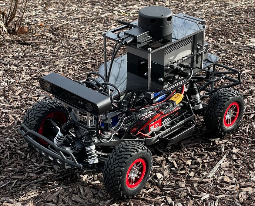
Figure 1: XTENTH-CAR wheeled mobile robot.

The platform is equipped with a 2D planar LiDAR, stereo camera, Inertial Measurement Unit (IMU), barometer, magnetometer and two batteries that each power the actuators and computer for increased run time for up to 2 hours on a single charge. The trained DRL policy utilizes under 25% of the available CPU and memory resources enabling smooth operation at high speeds and sampling rates.

III-B Simulator

AUTOnomous ground Vehicle deep Reinforcement Learning simulator (AutoVRL) [44] packages high fidelity environment models and a digital twin of XTENTH-CAR, illustrated in Figure 2, generated using Unified Robot Description Format (URDF) files with the open source Bullet physics engine [45]. DRL algorithms are implemented using Stable Baselines3 [46] which utilizes the PyTorch Machine Learning (ML) framework [47] interfaced with the physics engine using the Gym Application Programming Interface (API) [48].

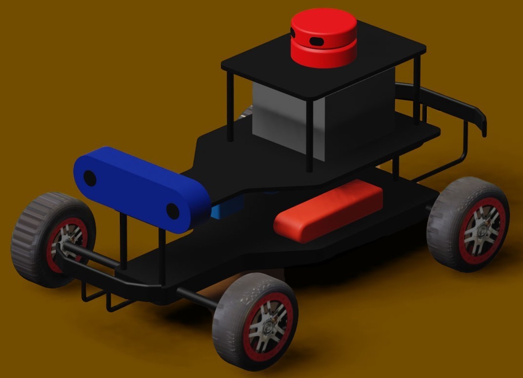
Figure 2: XTENTH-CAR digital twin.

AutoVRL includes implementations of GPS, IMU, LiDAR and camera sensors among which the 2D planar LiDAR was used for this work. Light transport and detection are modeled using ray tracing [49] to match real-world physics.

The LiDAR ray origin coordinates $(x_{RF},y_{RF},z_{RF})$ were computed as follows where $x_{L,A}$, $y_{L,A}$ and $z_{L,A}$ are coordinates of the LiDAR with respect to the AMR’s body frame, $x_{A}$, $y_{A}$ and $z_{A}$ represent the position of the AMR in the global coordinate frame, and $\psi_{A}$ is the AMR’s yaw,

$$x_{RF}=x_{L,A}cos(\psi_{A})+x_{A}$$ (1)

$$y_{RF}=y_{L,A}sin(\psi_{A})+y_{A}$$ (2)

$$z_{RF}=z_{L,A}+z_{A}$$ (3)

The end positions of $n$ rays $(x_{RT},y_{RT},z_{RT})$ each with a maximum ray length of $r_{max}$ were computed as follows where $(\frac{\pi}{4}-\psi_{A})$ is the LiDAR’s orientation, and $\alpha(\frac{1:n}{n})$ segments the Field of View (FoV) $\alpha$ into $n$ equally spaced rays,

$$x_{RT}=r_{max}sin\left((\frac{\pi}{4}-\psi_{A})+\alpha(\frac{1:n}{n})\right)$$ (4)

$$y_{RT}=r_{max}cos\left((\frac{\pi}{4}-\psi_{A})+\alpha(\frac{1:n}{n})\right)$$ (5)

$$z_{RT}=z_{L,A}$$ (6)

The start and end ray coordinates were used as inputs to the physics engine’s ray tracing function to obtain the object hit position of each ray $(x_{HP},y_{HP})$ using which the euclidean distance from the LiDAR’s position to detected obstacles $r_{o}$ was determined as follows,

$$r_{o}=\sqrt{(x_{HP}-x_{RF})^{2}+(y_{HP}-y_{RF})^{2}}$$ (7)

Actuator control inputs were applied to the joints of the simulated mobile robot using the physics engine’s motor control function. The steering angle was applied to two hinges, and velocity to the four tires.

The joint velocity for the current time step $v_{j,i}$ was computed as follows where $v_{j,i-1}$ is the joint velocity from the previous time step, $\dot{v}_{j,i}$ is the joint acceleration and $t_{s}$ is the sampling time,

$$v_{j,i}=v_{j,i-1}+t_{s}\dot{v_{j,i}}$$ (8)

The joint acceleration was computed from the throttle input $T$, throttle constant $C_{T}$ and resistive force $f$,

$$\dot{v}_{j,i}=C_{T}T-f$$ (9)

The resistive force $f$ was computed using constants $C_{f1}$ and $C_{f2}$ to improve the fidelity of the simulated action,

$$f=v_{j,i-1}(v_{j,i-1}C_{f1}+C_{f2})$$ (10)

Constants $C_{T}$, $C_{f1}$ and $C_{f2}$ are variable parameters utilized to tune rate of acceleration, and terrain resistance.

IV METHOD

The DRL policy $\pi_{\theta}(a_{t}\mid\mathcal{O}_{t})$ was trained using Proximal Policy Optimization (PPO) [50], an online on-policy actor-critic algorithm [51], to compute continuous actions in action space $a$ for continuous observations in observation space $\mathcal{O}$ at each discrete time step $t$, to maximize expected future rewards utilizing a DNN parameterized with weights $\theta$. The algorithm approximately maximizes the objective function $L_{t}(\theta)$ each iteration utilizing stochastic gradient ascent, where $\hat{\mathbb{E}}_{t}$ represents the empirical average for a finite batch of samples, $c_{1}$ and $c_{2}$ are coefficients, and $S$ is an entropy bonus to augment the objective to ensure exploration,

$$L_{t}(\theta)=\hat{\mathbb{E}}_{t}[L_{t}^{CLIP}(\theta)-c_{1}L_{t}^{VF}(\theta)+c_{2}S[\pi_{\theta}](\mathcal{O}_{t})]$$ (11)

The actor and critic networks each comprise 2 fully connected layers with 64 nodes each with $tanh$ activation that share parameters for efficient computation. The policy objective function $L_{t}^{CLIP}(\theta)$ utilized by the actor network is computed as follows, where $r_{t}(\theta)=\frac{\pi_{\theta}(a_{t}|\mathcal{O}_{t})}{\pi_{\theta old}(a_{t}|\mathcal{O}_{t})}$, $\epsilon$ is a hyperparameter, and $\hat{A}_{t}$ is an estimator for the advantage function computed over $T$ timesteps using discount factor $\gamma$,

$$L_{t}^{CLIP}(\theta)=\hat{\mathbb{E}}_{t}[\min(r_{t}(\theta)\hat{A_{t}},\text{clip}(r_{t}(\theta),1-\epsilon,1+\epsilon)\hat{A}_{t})]$$ (12)

The probability ratio $r_{t}(\theta)$ is clipped to avoid excessively large updates to the policy. The value function squared-error loss $L_{t}^{VF}(\theta)$ utilized by the critic network is computed as follows,

$$L_{t}^{VF}(\theta)=(V_{\theta}(\mathcal{O}_{t})-V^{target}_{t})^{2}$$ (13)

The actor selects actions to maximize the expected return of the policy, while the critic evaluates the quality of the chosen actions by minimizing the error between the estimated return $V^{target}_{t}$ and the actual return $V_{\theta}(\mathcal{O}_{t})$ during training. Post training completion, the actor network is solely used during inference to compute actions for each observation. Figure 3 illustrates the training and deployment schematic. The model is trained in simulation in a constrained racetrack to navigate the environment time-optimally at physical limits, and transferred zero-shot to the real-world for out-of-distribution generalization to new racetrack layouts, navigation in unstructured terrain, and dynamic obstacle avoidance.

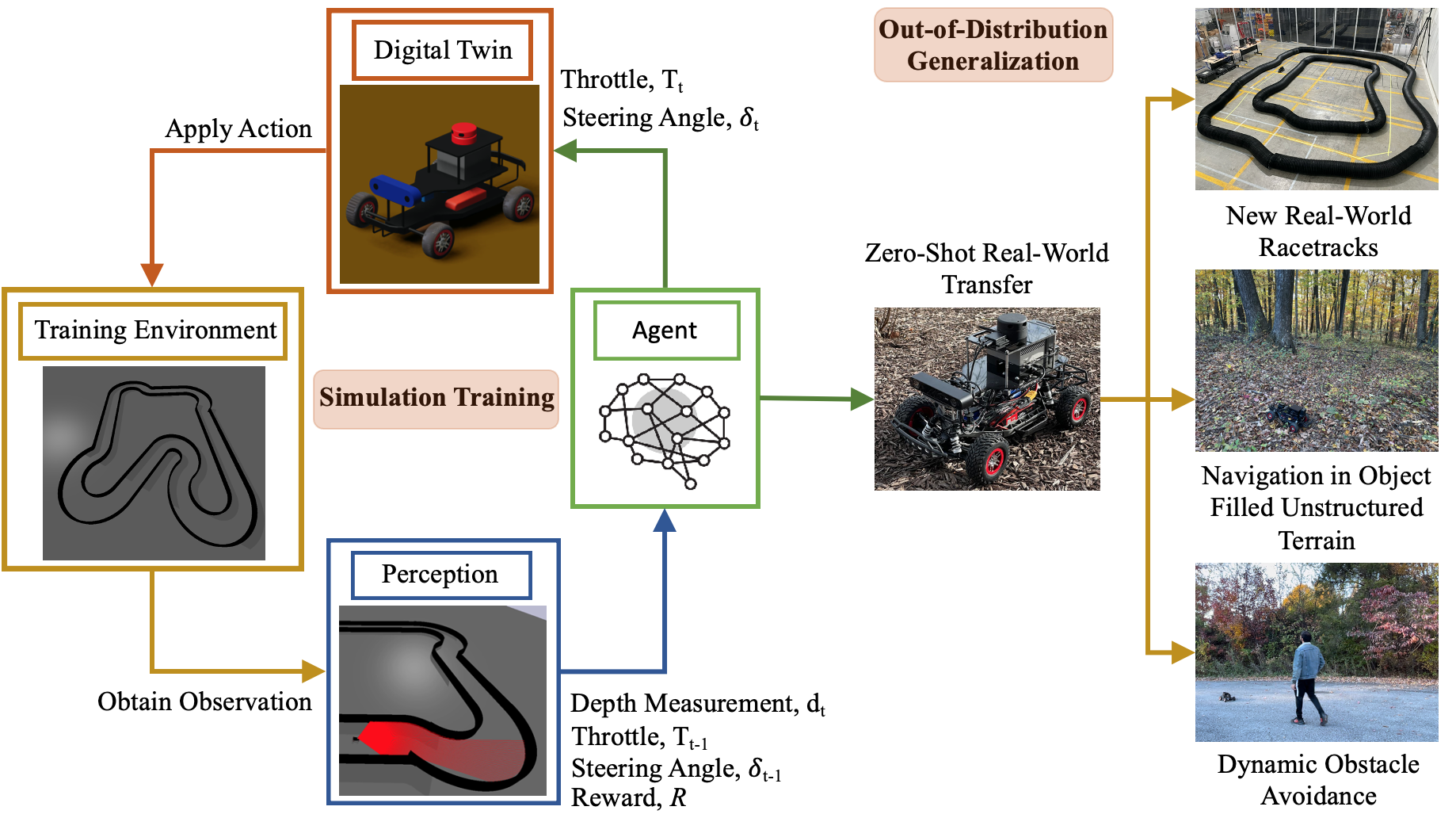
Figure 3: Methodology for training and deployment. The DRL model was trained in simulation in a constrained racetrack at physical limits and transferred zero-shot to the real-world for out-of-distribution generalization to new racetrack layouts, exploration in unstructured terrain and dynamic obstacle avoidance.

IV-A Observation Space

Depth observations that can be obtained using LiDAR or camera RGB-D point cloud were used as observations since these provide a complete spatial understanding of the surrounding environment at a fraction of the data size of RGB images enabling faster learning of policies, and efficient real time execution, similar to animals that use echolocation as a result of natural evolution, such as bats [52]. Moreover, the domain gap between simulation and real-world depth measurements is substantially smaller than for images which facilitates more accurate end-to-end policy transfer without high-level feature extraction from raw sensor inputs. The observation space $\mathcal{O}$ is defined as follows where $d_{i}$ is the depth measurement at each angle increment in the observation FoV,

$$\mathcal{O}=[d_{i}]^{1\times 170}$$ (14)

The 1D observation space comprises 170 depth measurements spread across a frontal $120^{\circ}$ FoV. The size of the observation space was found to have a significant effect on the learning ability of the agent. Higher resolution observations with 1000 measurements resulted in substantially slower learning and an inability to converge due to the less pronounced differences during object detection. Conversely, low resolution observations with 100 measurements were prone to missing small objects. The minimum resolution of 170, determined through empirical experimentation, provided sufficient detail for detection of small objects with a 5 $cm$ radius with pronounced alteration in the space for detected object profiles that enabled quick learning of accurate behavior. A frontal $120^{\circ}$ FoV was chosen over a $360^{\circ}$ FoV to also enable faster learning of desirable behavior as a consequence of the agent being more focused on objects directly in front. Larger FoVs took longer to converge, and did not improve obstacle avoidance ability or exploration efficiency. This matches natural evolution where animals perceive the surrounding environment without compromise efficiently with a limited FoV.

IV-B Action Space

The DRL algorithm selects normalized continuous actions $a_{T}$ and $a_{\delta}$ in the range [-1 1] for each observation. The two dimensional vector action space a is defined as follows,

$$\textit{a}=(a_{T},a_{\delta});\;\;\;\;a_{T},a_{\delta}\in[-1,1]$$ (15)

High-level control inputs, throttle $T$ in the range [0 1], and steering angle $\delta$ in the range $[\delta_{min}\delta_{max}]$ were computed from the normalized actions as follows,

$$T=min(max(a_{T},0),1)$$ (16)

$$\delta=max(min(a_{\delta},\delta_{max}),\delta_{min})$$ (17)

Throttle control commands were linearly mapped to the AMR’s linear velocity. No further processing was performed on the steering control inputs.

IV-C Reward Formulation

Shaped and sparse rewards were tested with the former penalizing collisions and states close to racetrack boundaries in addition to rewarding the square of the throttle output, and the latter solely rewarding high throttle output. The sparse reward was found to perform better, yielding optimal trajectories in simulation. The shaped reward resulted in excessive wall avoidance behavior that slowed lap time. The optimal reward formulation $T^{2}$ maximized velocity at each state subject to the AMR’s unknown dynamics, however resulted in excessive swerving when transferred to the real-world. To correct this, the following reward was formulated where $a_{\delta,prev}$ and $a_{\delta,curr}$ are unprocessed steering angles determined by the learning agent at the previous and current time steps,

$$R=\begin{dcases}5T^{2}&\\ -2.0&\text{if }a_{\delta,prev}a_{\delta,curr}=-1\\ \end{dcases}$$ (18)

The product of the previous and current steering angle outputs was penalized if it was negative at the upper bound to mitigate imperfections in the physics engine that the agent exploited during accelerated training to learn rapidly oscillating steering angle outputs. The correction component was formulated after observing the initial policy transfer and error patterns to re-train the model with the difference between simulator and real-world physics accounted for, which resulted in no increase in training time or performance in simulation, but transferred zero-shot to the real-world. The weights of each reward component were chosen to prioritize maximizing the throttle output for time-optimal performance.

IV-D Training and Evaluation

Training was performed in a handcrafted multidirectional racetrack with varying cornering radii, as illustrated in Figure 4, using an Intel Core i9 13900KF CPU and NVIDIA GeForce RTX 4090 GPU for 20,000,000 steps that corresponded to 15,747 training episodes, accelerated at 30 times real-time speed, in 48 wall-clock hours. An episode concluded when the agent collided with the racetrack boundary, following which it was reset to the same starting position.

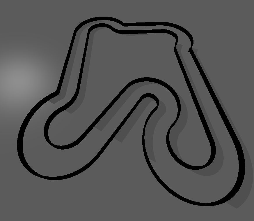
Figure 4: Multidirectional racetrack used for training.

The mixture of turning directions and lengths prevented the model from overfitting to a specific layout to enable out-of-distribution generalization by providing an array of observation sequences in a constrained environment for learning of obstacle avoidance behavior at the maximum attainable velocity within the laws of physics, which required planning sequences of actions using detected object profiles, that facilitated dynamic obstacle avoidance at a sufficient sampling rate. The hyperparameters used for training are summarized in Table I.

TABLE I: Training Hyperparameters

Hyperparameter	Value
Discount Factor ($\gamma$)	0.99
Learning Rate	0.0003
Rollout Buffer Size	2048
Batch Size	64
Number of Epochs	10

Out-of-distribution generalization for navigation was tested in simulation in a densely cluttered 50$m$ x 50$m$ outdoor environment, illustrated in Figure 5, that included tree and boulder objects with explorable regions underneath that are unobservable to aerial surveillance, where ground AMRs are beneficial for exploration.

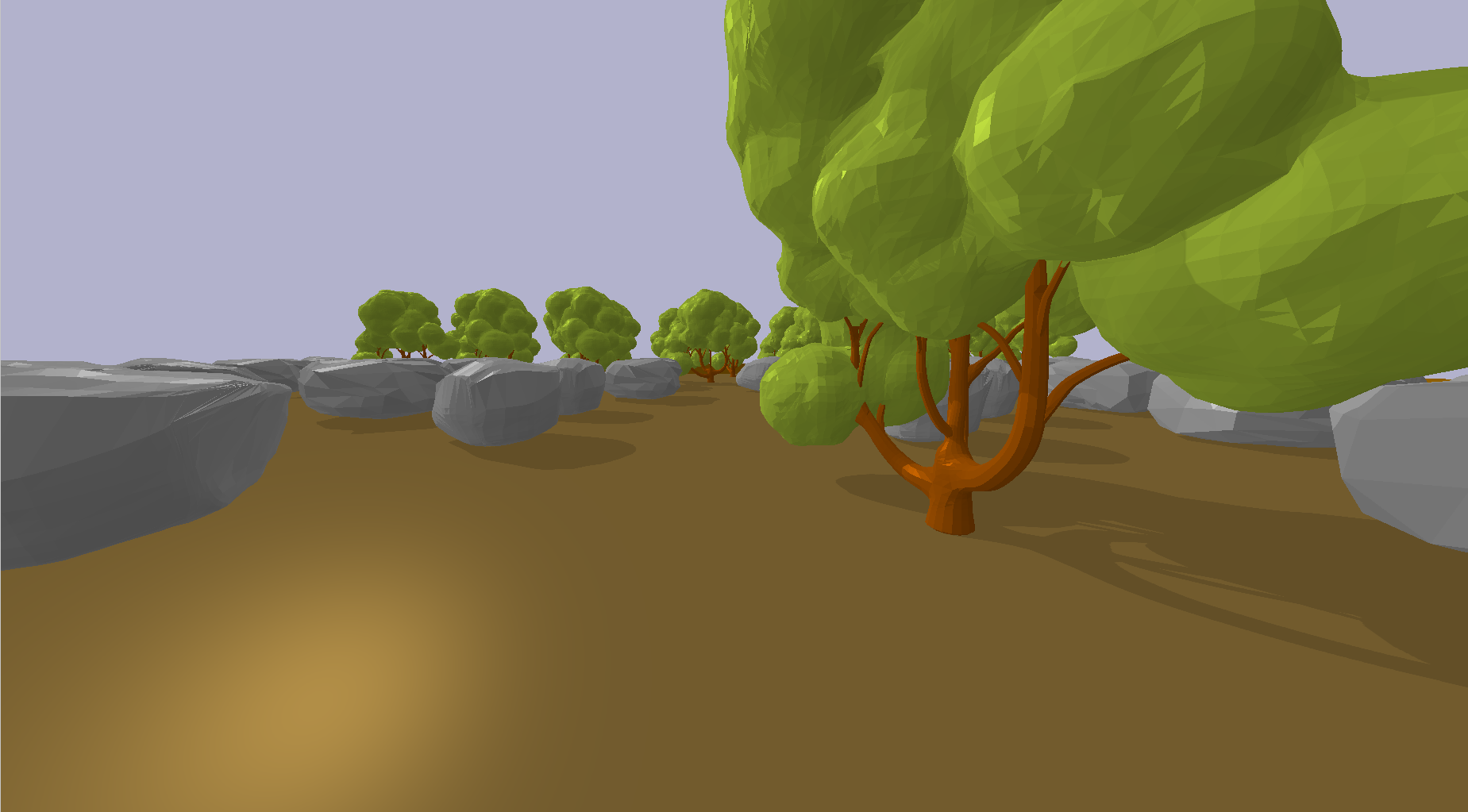
Figure 5: Simulated outdoor environment used for evaluation of out-of-distribution generalization.

Real-world policy transfer was tested in five scenarios that include racing in different racetrack layouts to the training environment, navigation in an object filled laboratory environment, evaluation of exploration behavior in a parking lot, navigation in unstructured forest terrain, and dynamic obstacle avoidance.

Racing performance was evaluated in three unknown racetracks with energy absorbent barriers, as depicted in Figure 6 to gauge zero-shot policy transfer, and generalization to new configurations outside the training distribution.

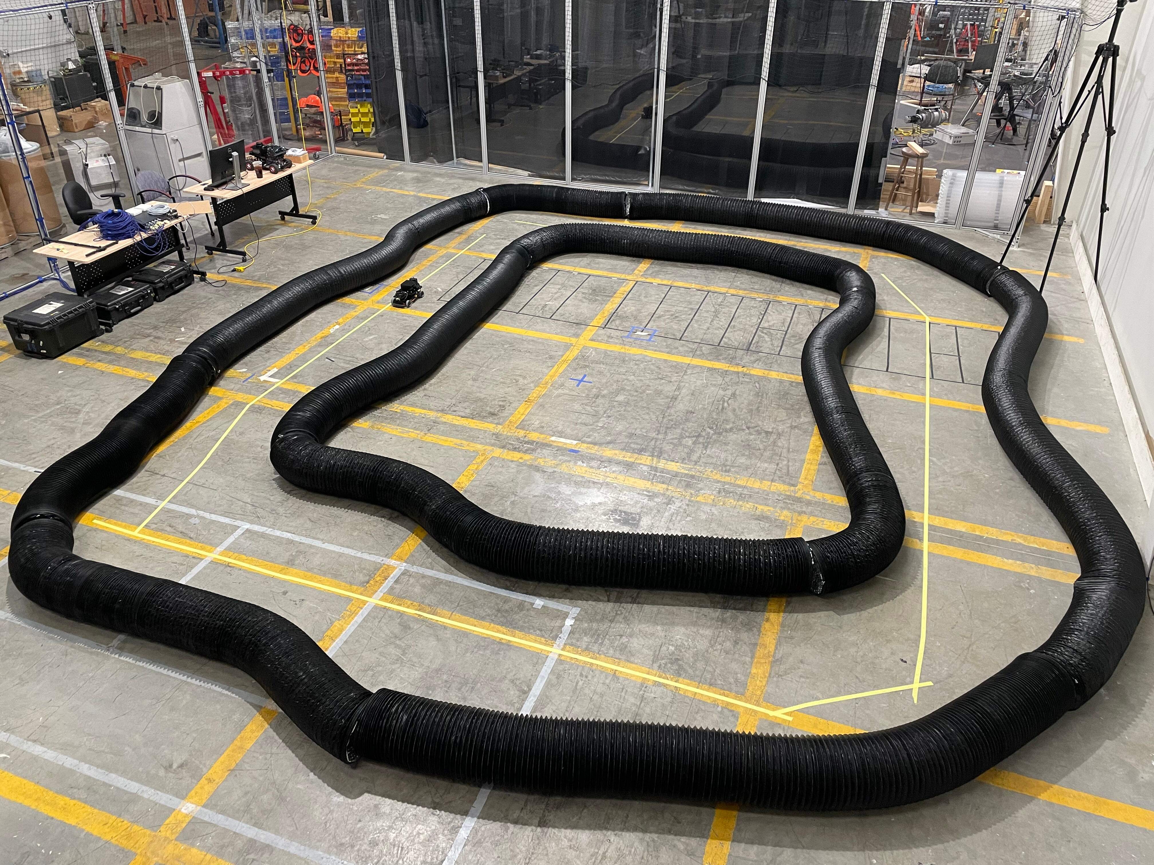
(a)

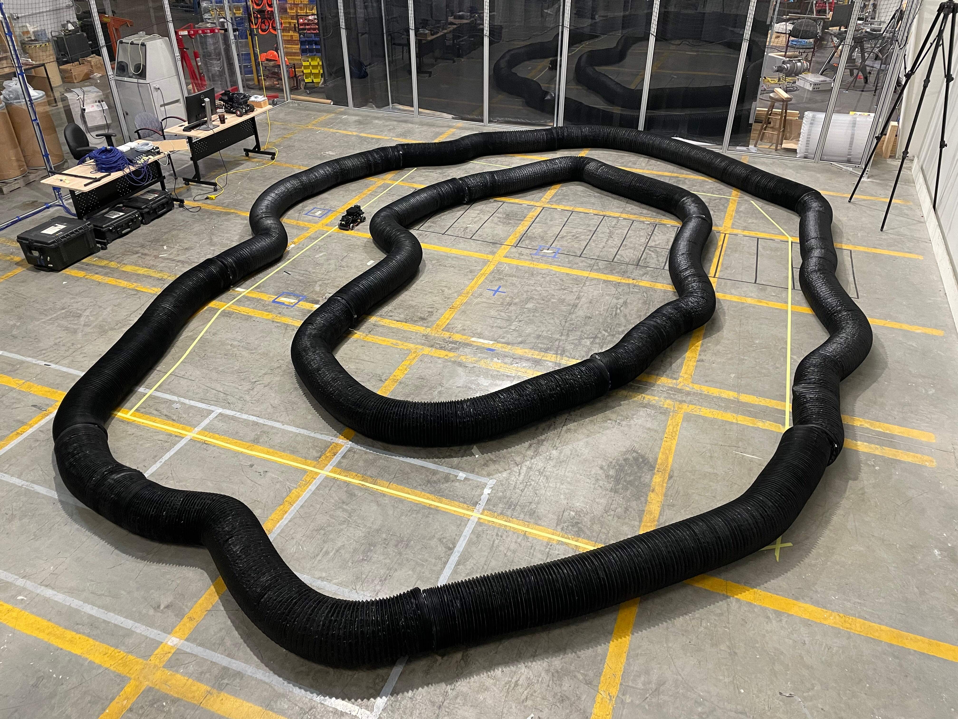
(b)

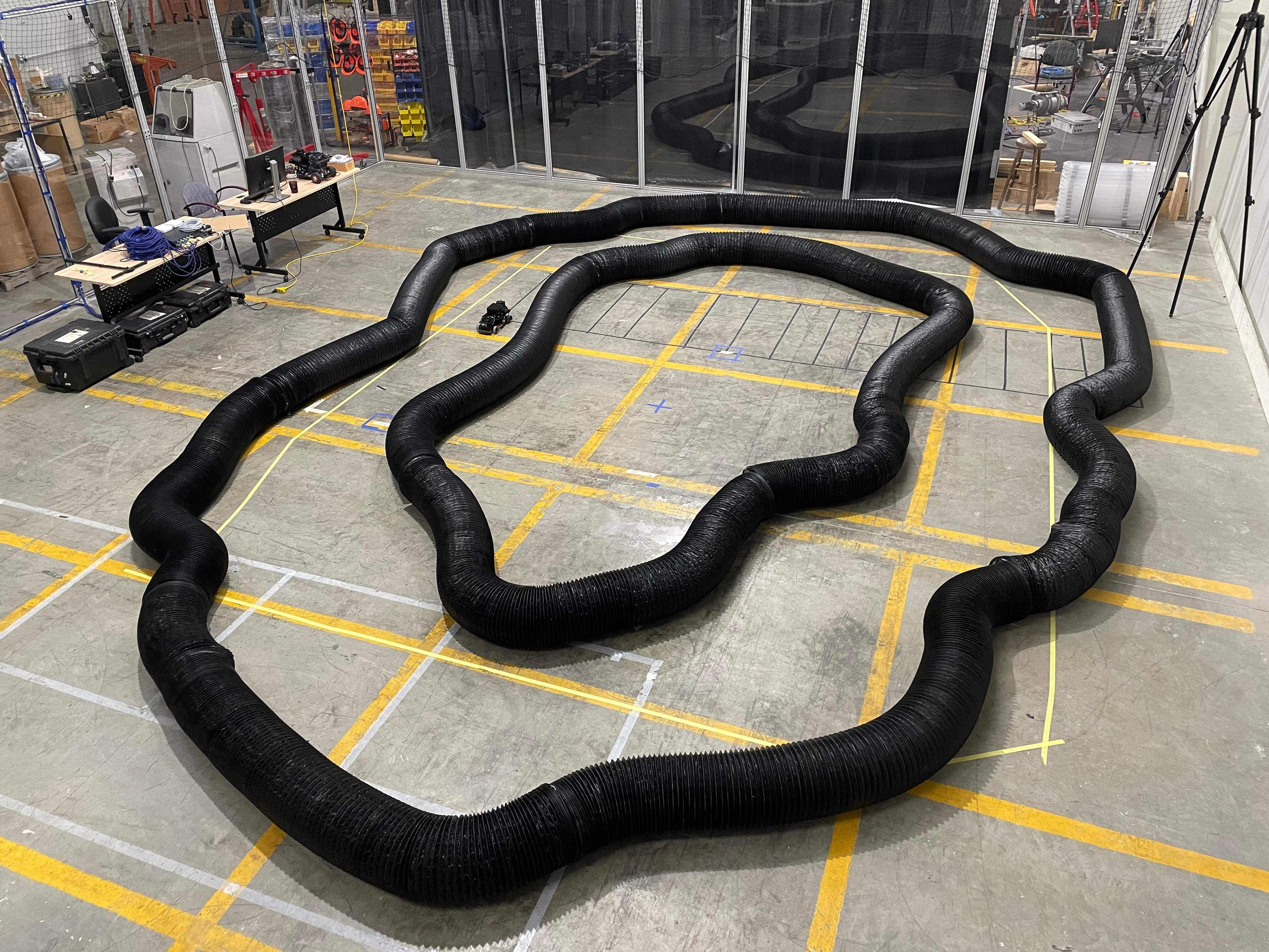
(c)

Figure 6: Real-world racetrack layouts used to evaluate zero-shot simulation to real-world policy transfer. (a) Straight and simple corners. (b) Long cornering length. (c) Multiple cornering directions in quick succession.

Out-of-distribution navigation capabilities were tested in a laboratory obstacle filled experimental environment depicted in Figure 7 that was populated with a range of obstacle shapes and sizes. Exploration behavior and efficiency were tested in a parking lot, illustrated in Figure 7, and robustness in unstructured terrain with increased sensor noise was evaluated in a forest, depicted in Figure 7. Dynamic obstacle avoidance was evaluated for social navigation for pedestrian avoidance at an operation speed of 1$m/s$.

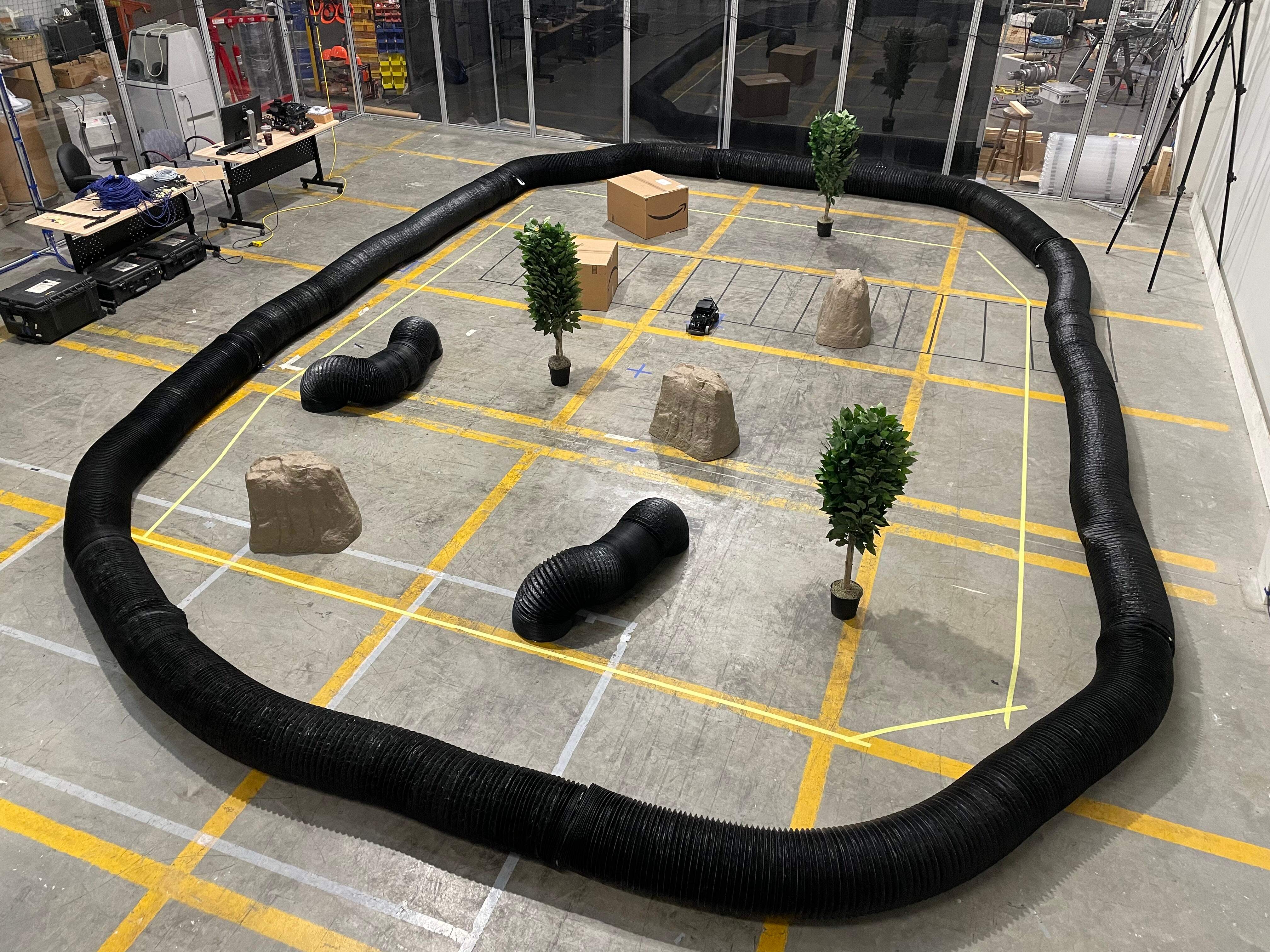
(a)

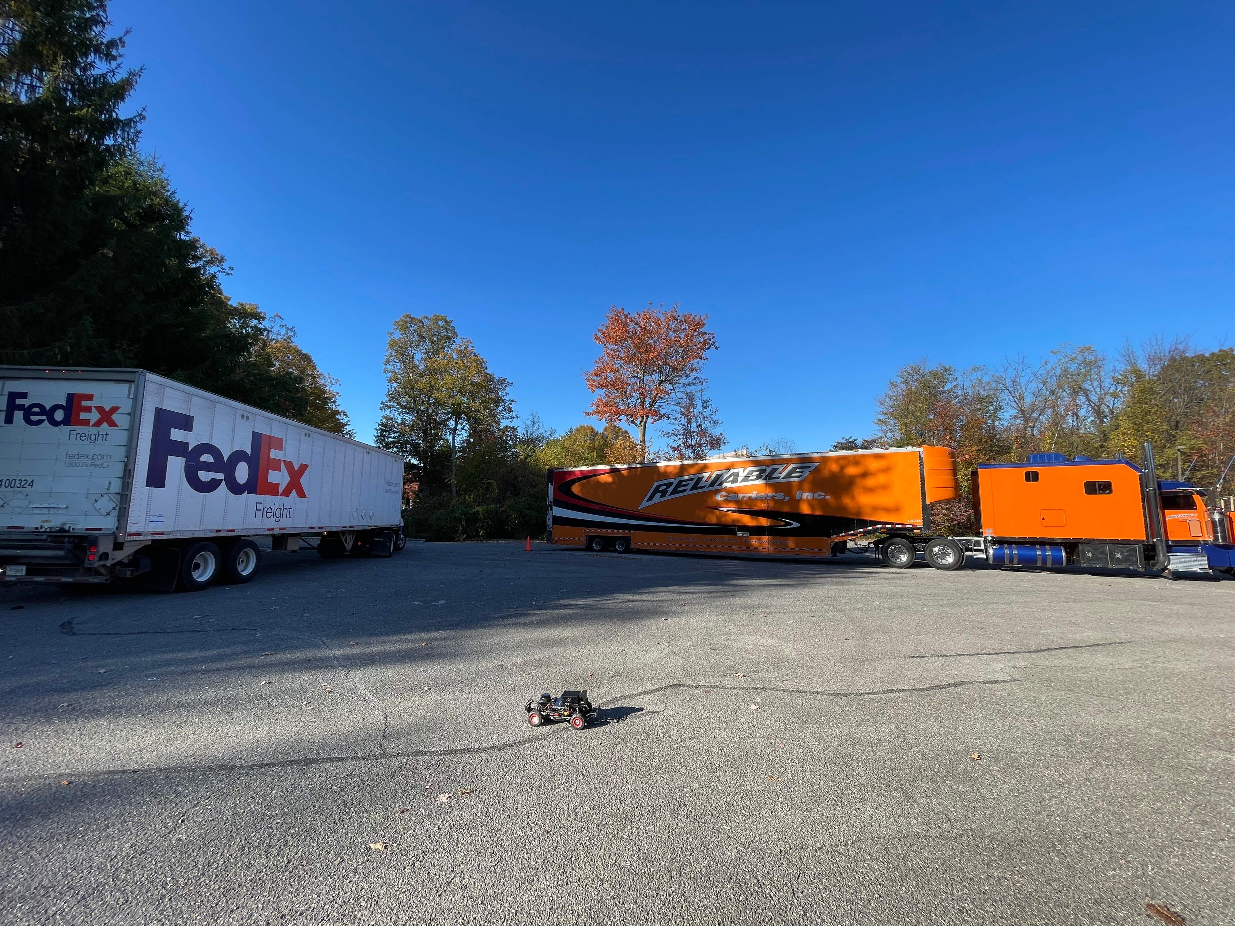
(b)

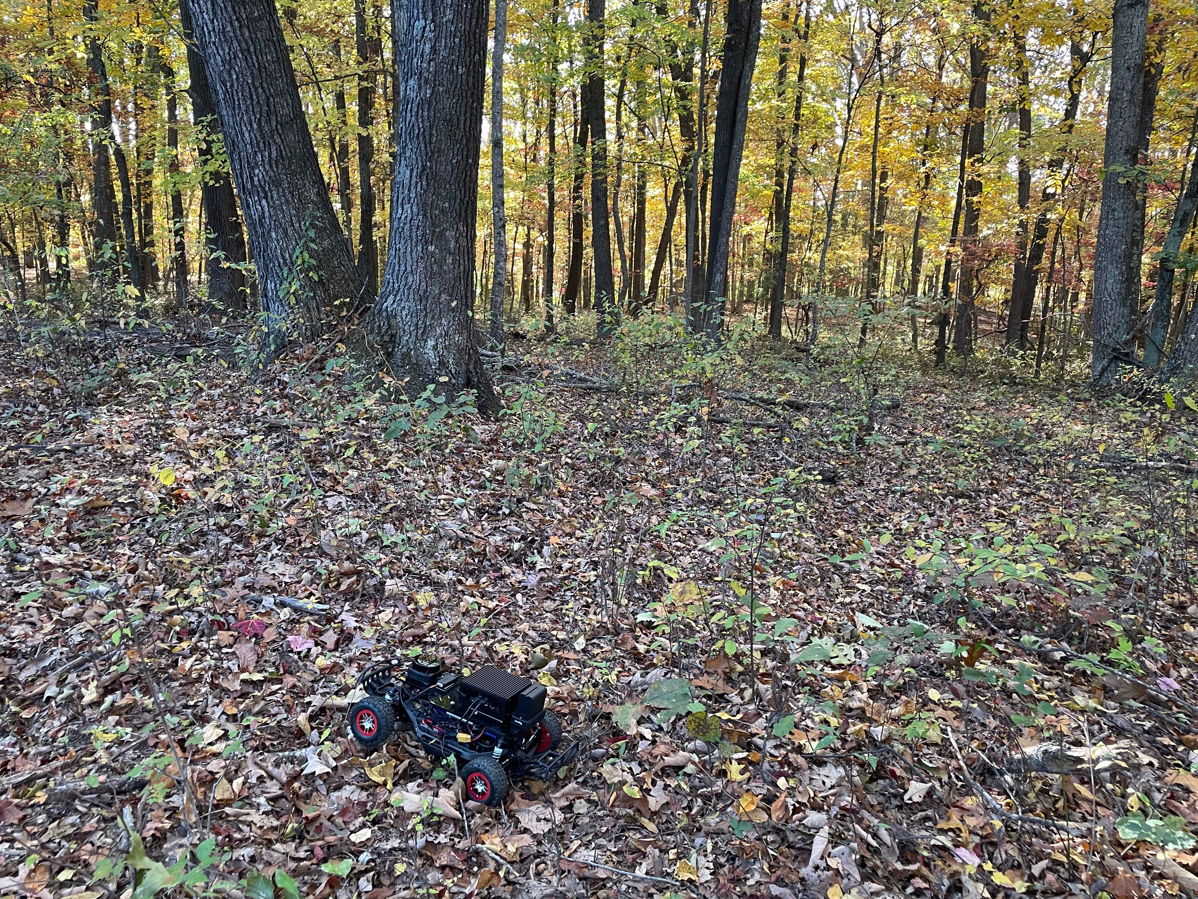
(c)

Figure 7: Environments used to evaluate exploration without a-priori maps. (a) Laboratory obstacle filled experimental environment. (b) Parking lot. (c) Forest.

V RESULTS

This section presents the simulation and real-world results. The project video can be viewed at: https://youtu.be/jUtPaQV3Bd8.

V-A Learning Curve

The learning curve during training is illustrated in Figure 8 where the order 1000 moving average reward is plotted against the training episode.

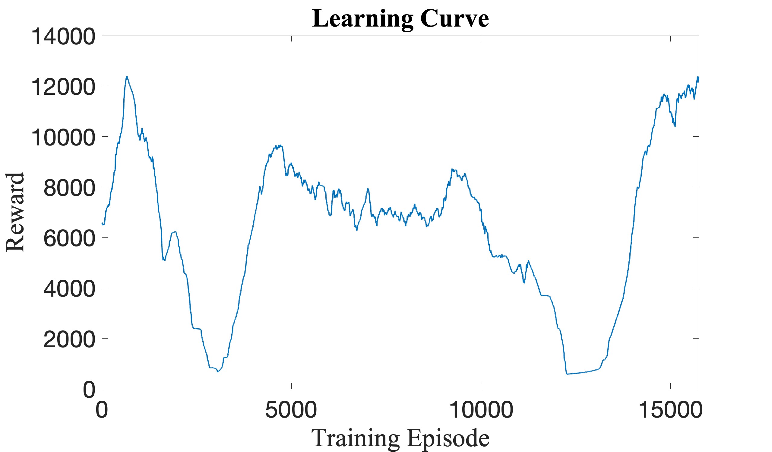
Figure 8: Order 1000 moving average reward each training episode.

An average reward of 12,383 was attained post training completion. The learning curve is highly nonlinear, similar to non-trivial environments in prior work [15, 53]. At episode 657, a high reward was obtained, however, the policy was overfitted at this point, since the agent was unable to replicate results consistently as can be observed when the average reward drops with further training, as different action sequences were experimented to collect training samples to improve the long term cumulative return.

At episode 4,675, a local maximum was attained at which point the trained policy computed actions to navigate the racetrack with time-optimal trajectories for 2 laps before collision. To improve performance, training was continued, during which the average reward was constant for 4,900 episodes at the local maximum, after which at episode 9575, further action sequences were experimented to learn an optimal policy at the end of the training period at episode 15,747. The policy learned at the end of the nonlinear learning curve mapped observations to actions to navigate the racetrack safely without collision for 20 tested laps, with the same time-optimal trajectory solved at the local maximum.

V-B Performance in Training Environment

The time-optimal post training trajectory in the racetrack used for training is depicted in Figure 9.

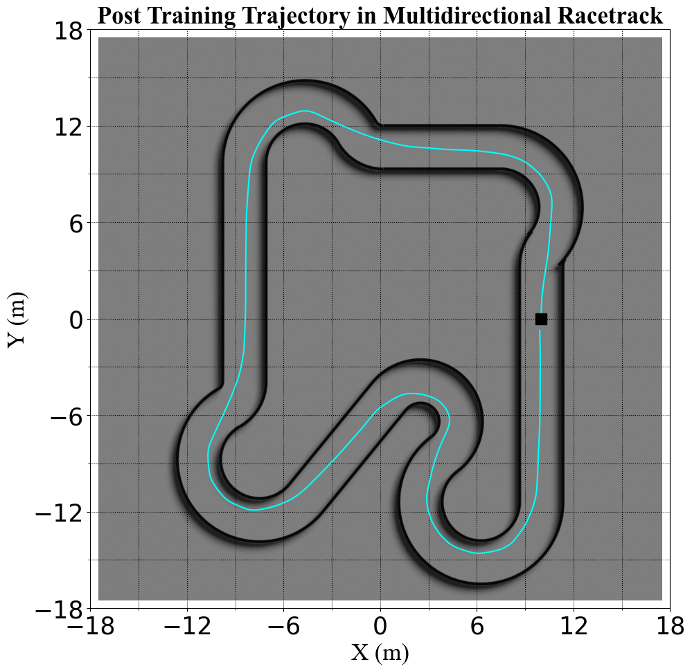
Figure 9: Time-optimal trajectory in the multidirectional racetrack used for training.

Racing requires prediction and planning to execute control signals in sequence to maximize velocity at physical limits in highly nonlinear domains. The learned policy selected actions at these limits to navigate multiple turns of varying directions and radii conforming to an optimal racing trajectory that navigated to the apex of each corner to traverse the shorter inside region to minimize lap time, identical to professional racing drivers.

Unlike conventional racing algorithms that use optimization methods such as Model Predictive Control (MPC) and sampling methods such as Rapid Random Trees (RRT) [54, 55], the DRL model computed control inputs using significantly fewer operations, and did not require prior maps or track boundary information.

V-C Out-of-Distribution Generalization for Navigation in Simulated Outdoor Environment

The racing agent exhibited emergent behavior that extended to navigation in obstacle filled environments. Out-of-distribution generalization for navigation in the 50$m$ x 50$m$ simulated outdoor environment is illustrated in Figure 10.

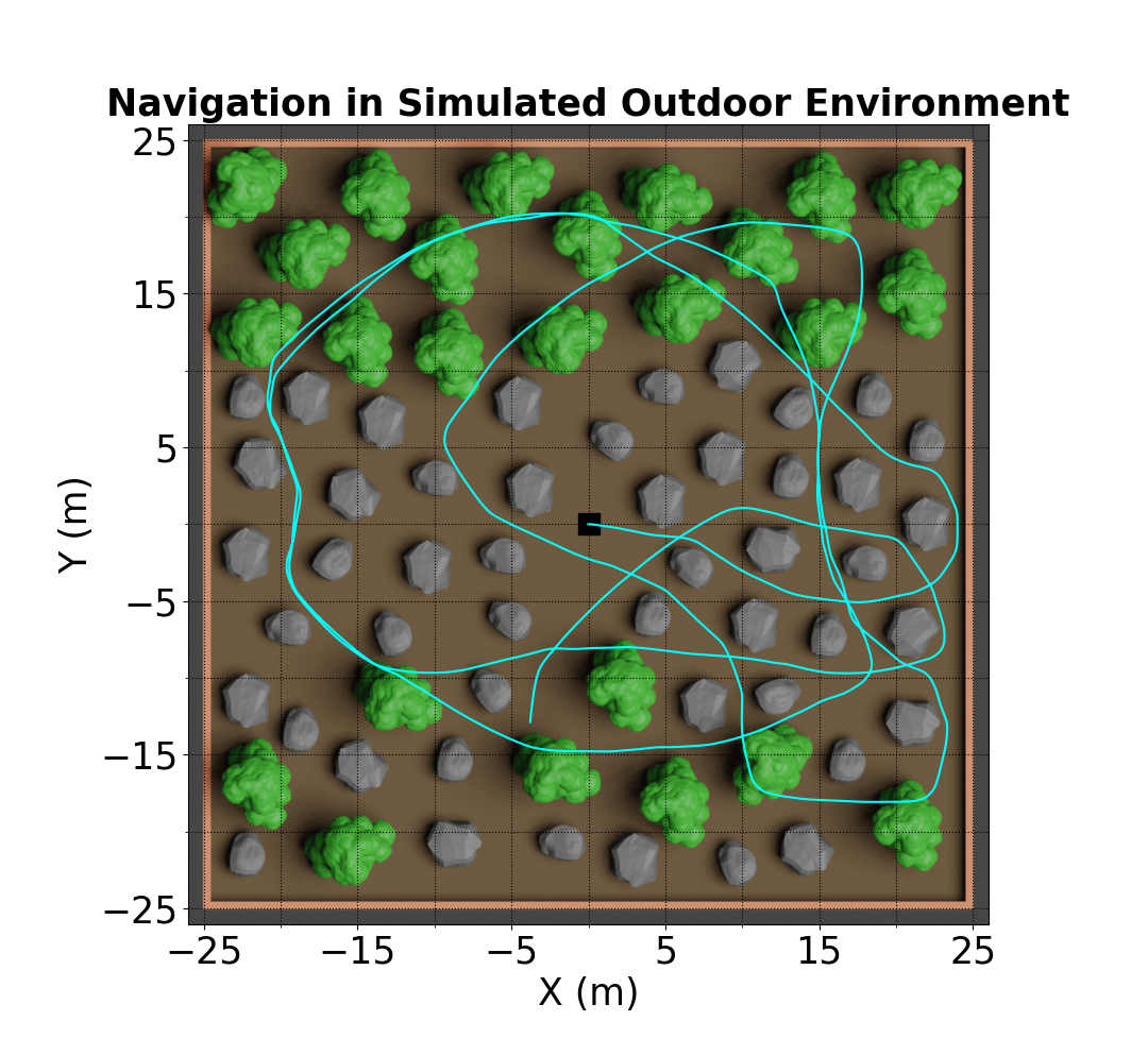
Figure 10: Out-of-distribution generalization for navigation in the simulated outdoor environment.

The policy trained to race in 20,000,000 steps explored this environment more effectively than policies trained in 60,000,000 steps using PPO or Soft Actor-Critic (SAC) [56] with different variations of the shaped reward in [15] specifically designed for exploration in obstacle filled environments without prior maps. SAC outperformed PPO when trained directly in the object filled environment, with the latter learning inefficient circular motion in the same vicinity despite the addition of a penalty to the reward for excessive steering inputs. In contrast, PPO learned a better policy in the racetrack environment where there were more pronounced alterations in the observation space, in which SAC took longer to converge, and did not learn the time-optimal trajectory due to more emphasis on exploratory behavior that led to conservative racetrack boundary avoidance.

The constrained racetrack environment with sparse rewards resulted in more rigorous training that enabled learning of desirable obstacle avoidance behavior with a higher success rate and three times fewer training samples than training in obstacle filled environments with shaped rewards. Moreover, the racing policy facilitated obstacle seeking behavior that is beneficial to ground AMRs for exploration and search applications in aerially occluded regions.

V-D Zero-Shot Real-World Transfer

The policy learned in simulation was transferred zero-shot to the physical AMR, with no additional training in the real-world. Planar LiDAR range measurements were processed to match the simulated observation space. Sensor and actuator noise were not modeled and added to simulation training, nor was domain randomization utilized.

Time-optimal, collision free trajectories traversed in the three tested racetracks are shown in Figure 11, demonstrating zero-shot policy transfer trained in simulation without safety considerations for uncompromised performance, and generalization to new multidirectional racetracks.

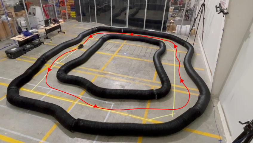
(a)

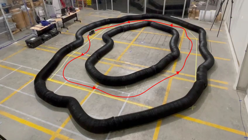
(b)

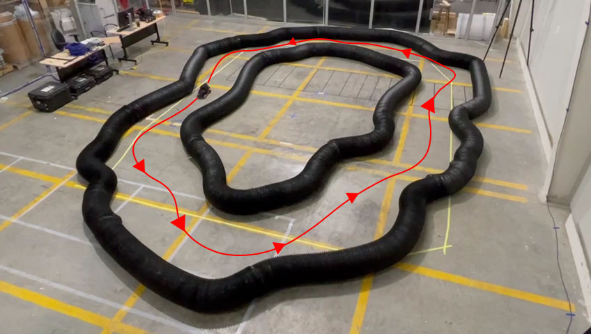
(c)

Figure 11: Trajectories in new real-world racetracks without prior maps. (a) Straight and simple corners. (b) Long cornering length. (c) Multiple cornering directions in quick succession.

The DRL model utilized less computation resources for better racing performance compared to a modified wall following PID controller and MPC combined with Artificial Potential Function (APF) [57], and lapped faster than non-expert humans with manual control. On average, the policy navigated the short racetracks 30% faster than the tested methods, while utilizing the same CPU usage as the PID controller, and half that of the optimization method.

The laboratory obstacle filled environment contained various objects of different profiles such as boulders, tubes and small pots. The trajectory for out-of-distribution generalization in the cluttered test environment is shown in Figure 12. The results demonstrate successful obstacle detection and avoidance, with high accuracy. Exploration was sufficient to collect data in all regions using onboard sensors, but can be further improved. The racing nature of the learned policy led to high risk obstacle avoidance behavior where the AMR charted trajectories to avoid obstacles at the last possible moment, and favored trajectories between obstacles, that is beneficial for exploration and search applications.

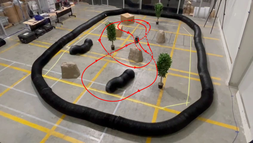
Figure 12: Exploration trajectory in the static object filled laboratory environment.

Exploration efficiency was further tested in a parking lot, shown in Figure 13. This environment had large regions of empty space with objects such as parked cars, trailers and paved risings that facilitated testing for deployment in urban settings for disaster relief or military operations. The AMR navigated the region without collision or repeated motion in the same vicinity, exhibiting efficient, and thorough exploration capability that demonstrates feasibility for autonomous deployment in environments without prior knowledge, or GPS coverage.

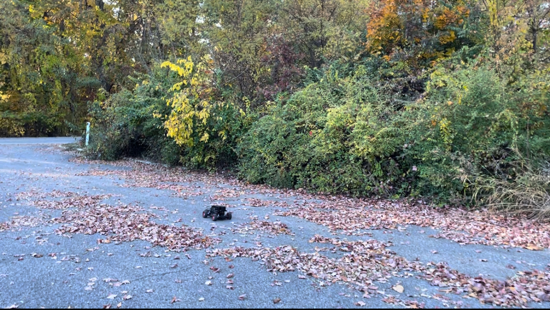
(a)

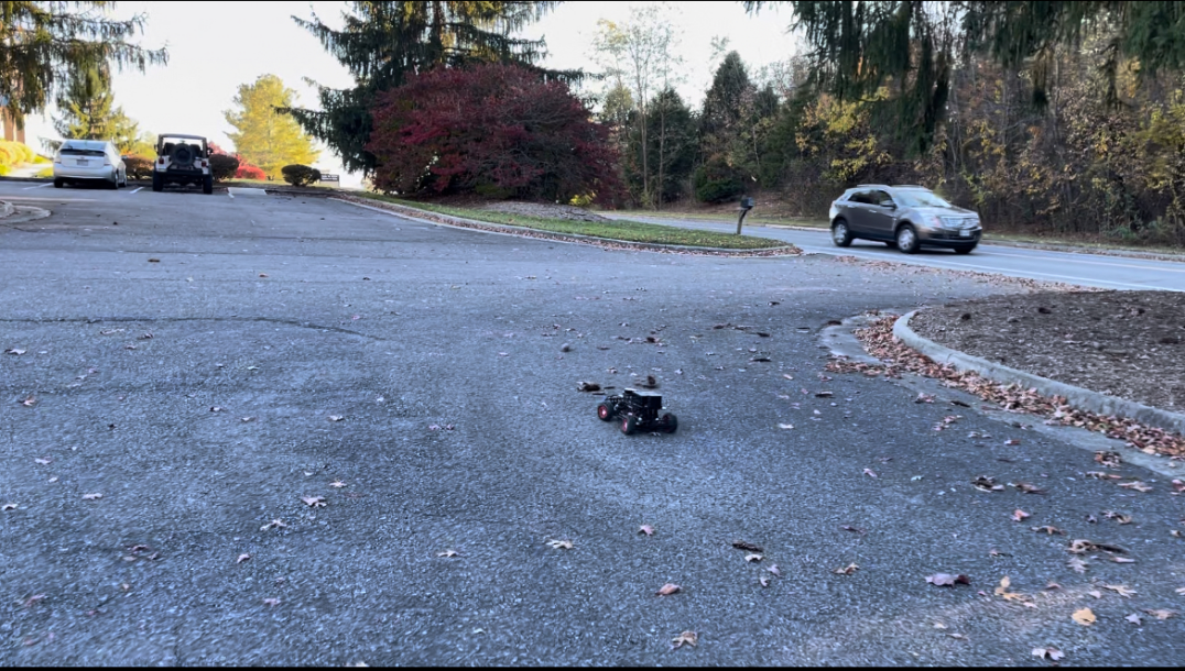
(b)

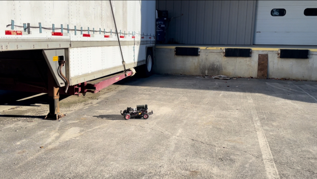
(c)

Figure 13: Exploration in a parking lot. (a) Intrinsic exploratory behavior. (b) Accurate obstacle avoidance. (c) Obstacle seeking behavior.

V-E Navigation in Unstructured Terrain

Robustness to increased sensor noise was tested in unstructured forest terrain that included vegetation, soil and leaf litter, shown in Figure 14. The AMR never collided with trees and branches during testing including narrow regions between sparsely detected branches, demonstrating strong resilience to added noise from changes in terrain elevation, and obstacle avoidance capability. The exploration trajectory was efficient, with new regions covered over the course of operation with no repeated coverage in the same vicinity, and the learned racing behavior was beneficial for improved search ability enabling navigation close to trees to seek and explore shaded regions that can be unobservable to aerial surveillance.

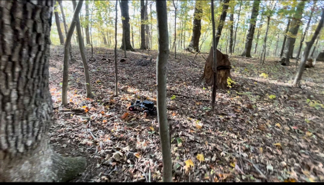
(a)

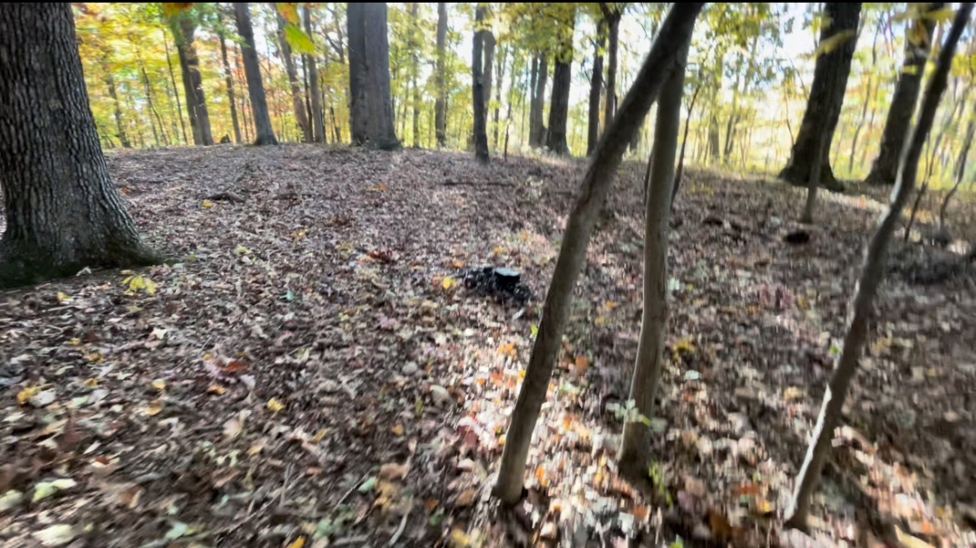
(b)

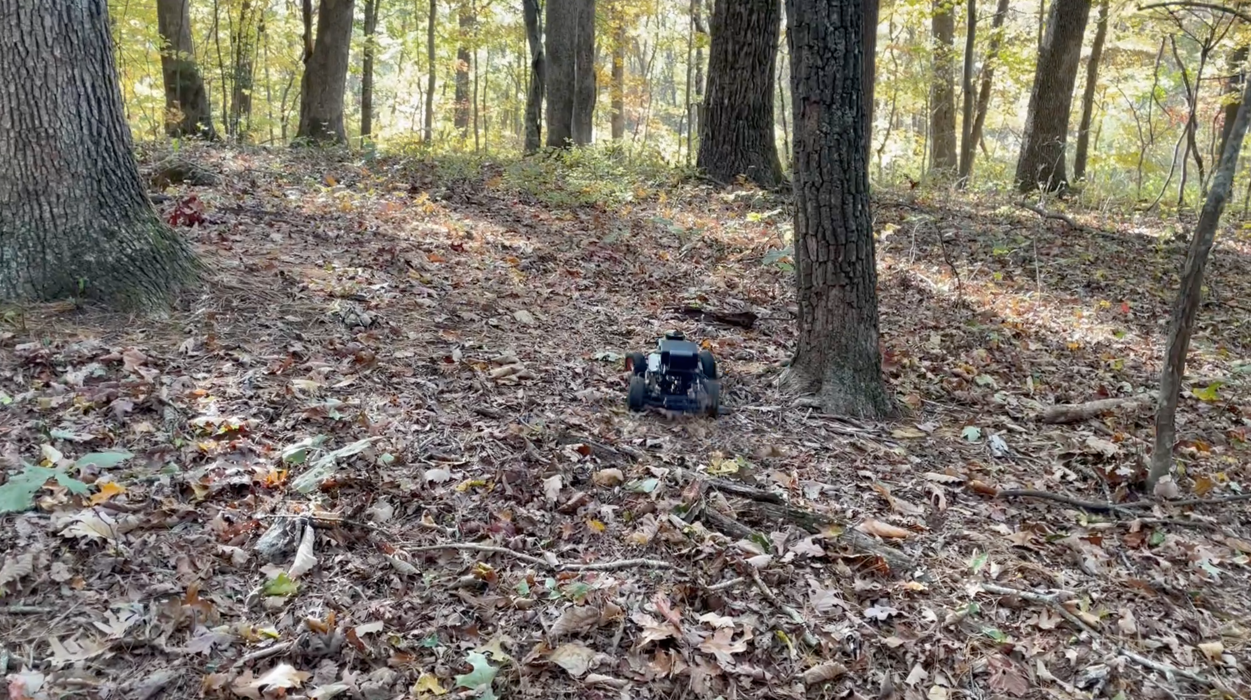
(c)

Figure 14: Exploration in unstructured forest terrain. (a) Navigation in narrow region between sparsely detected branches. (b) Avoidance of repeated motion in the same vicinity. (c) Obstacle seeking behavior that is beneficial for exploration of aerially occluded shaded regions.

The results demonstrate the effectiveness of the trained policy for SAR, military, and planetary exploration applications in hazardous regions inaccessible to humans. The method does not require a high-level planner to provide goal positions, as is necessary for conventional approaches which makes it more flexible and adaptable to various environments and applications, while maintaining high levels of safety and efficiency, enabling exploration and data collection in new, unknown environments for downstream tasks. An added benefit is the lack of computationally expensive SLAM algorithms that enables utility in high speed real-time applications, and execution on a range of AMRs with varying payloads for embedded computers.

V-F Out-of-Distribution Generalization for Dynamic Obstacle Avoidance

The learned behavior extended to dynamic obstacle avoidance outside the training distribution, where directions of dynamic objects influenced action outputs for collision free navigation. Three test scenarios for moving pedestrian avoidance are shown in Figures 15, 16 and 17.

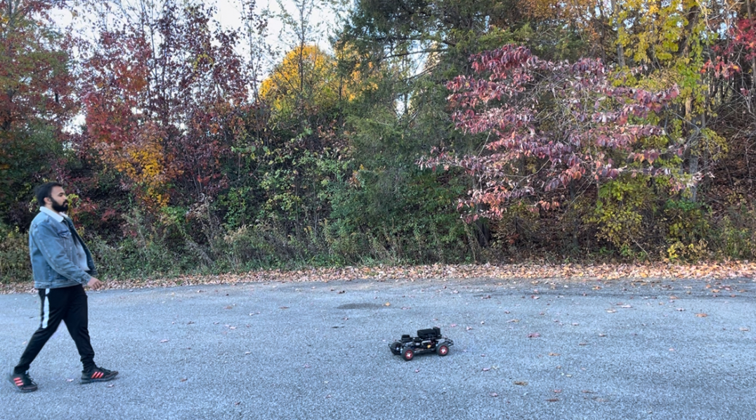
(a)

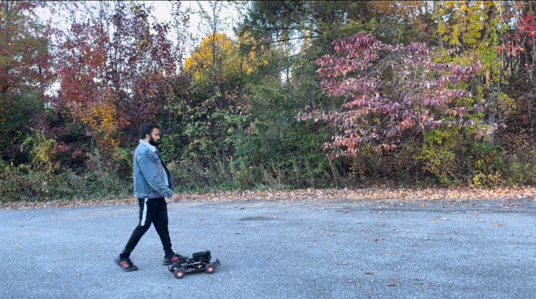
(b)

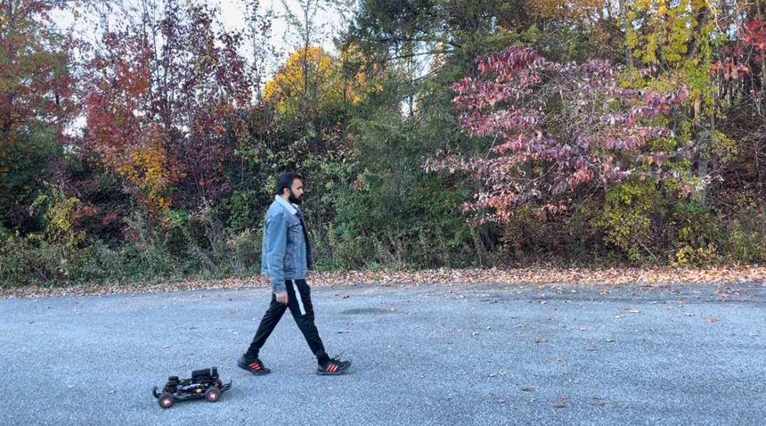
(c)

Figure 15: Dynamic pedestrian avoidance: Scenario 1. (a) Trajectories on collision course. (b) Evasive maneuver. (c) Dynamic obstacle avoided.

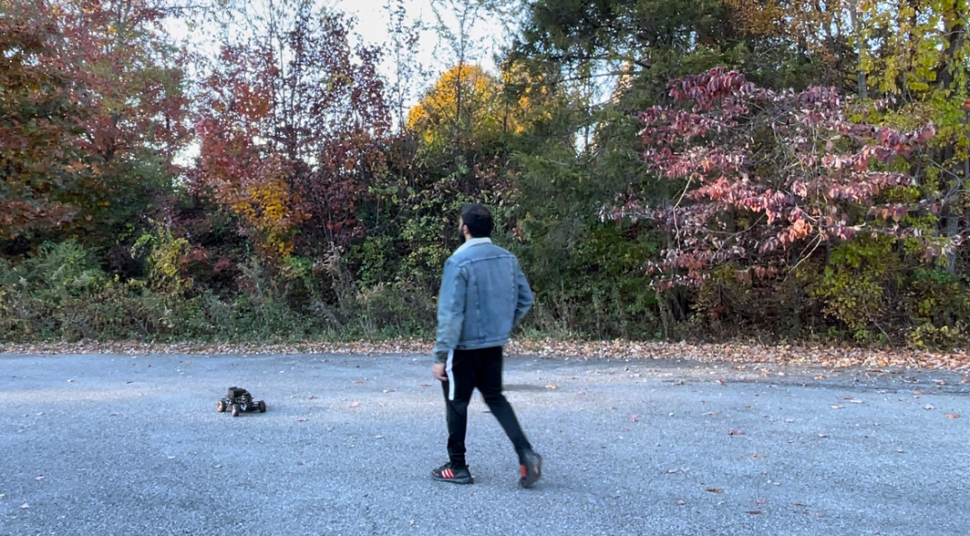
(a)

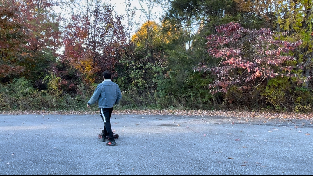
(b)

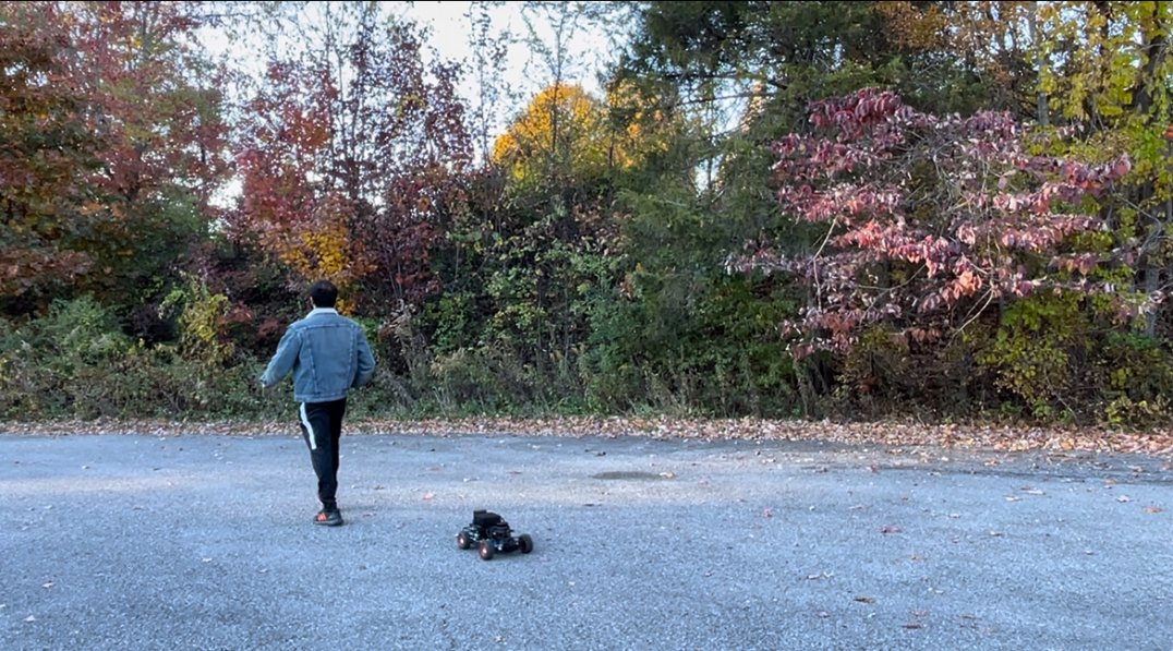
(c)

Figure 16: Dynamic pedestrian avoidance: Scenario 2. (a) Trajectories on collision course. (b) Evasive maneuver. (c) Dynamic obstacle avoided.

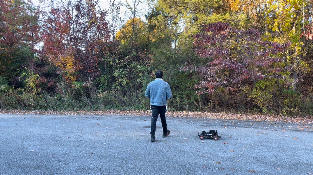
(a)

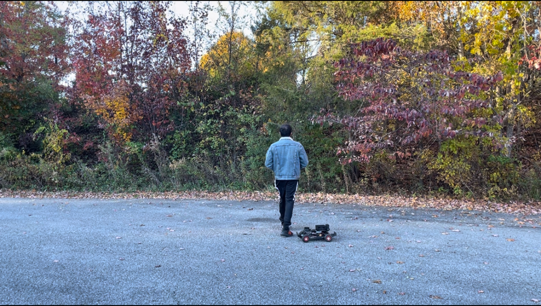
(b)

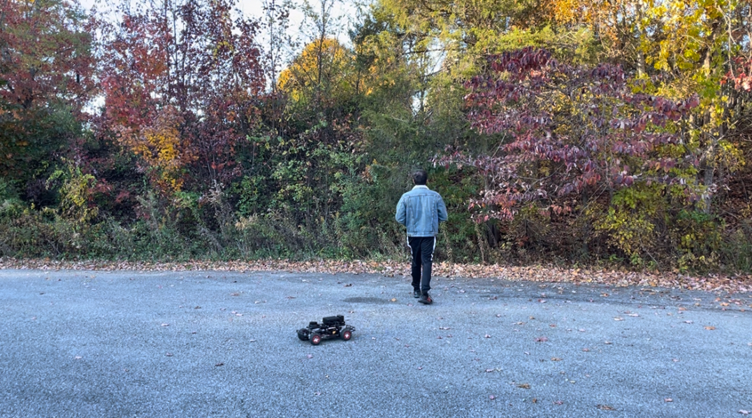
(c)

Figure 17: Dynamic pedestrian avoidance: Scenario 3. (a) Trajectories on collision course. (b) Evasive maneuver. (c) Dynamic obstacle avoided.

Prediction and planning required to execute control inputs in sequence to maximize velocity for racing at highly nonlinear physical limits transferred well to dynamic obstacle avoidance at a tested velocity of 1 $m/s$ that represents a typical AMR operation speed around humans.

VI DISCUSSION

VI-A Bridging the Simulation to Real-World Gap

15,747 collisions and resets were necessary for training completion which would have required significantly more time and labor in the real-world. Development of end-to-end DRL approaches is primarily limited by the lack of good simulation environments for simulation to real-world policy transfer. Depth measurements enable accurate policy transfer due to the accurate modeling in physics engines using ray tracing. Advances in neural surface reconstruction [58] have potential for photorealistic, detailed scene construction in simulators from RGB video recordings, to better bridge the reality gap for end-to-end policies that utilize image observations.

Adding perturbations to enhance robustness, and domain randomization are common methods used to bridge the reality gap, but both result in suboptimal policies that can require longer training times to converge. The trained policy was robust to sensor and actuator noise in different environment configurations, and terrain without modelled noise or randomized physics parameters during training. The use of a reward component to learn the difference between observed real-world and simulator physics optimized policy transfer for effective zero-shot adaptation without an increase in convergence time.

VI-B Emergent Behavior for Out-of-Distribution Generalization

The DRL model’s generalization capability is attributed to the learned representation that effectively captures the behavioral similarity between observations across various tasks, enabling the agent to adapt and perform in new environments. The policy captures the underlying structure of the perceived environment in a compact 2 layer DNN, that facilitates quick computation.

The results demonstrate the potential of AI agents to generalize to diverse and unrelated scenarios, and suggest that training in a constrained environment at physical limits can lead to more efficient training in a small parameter space, and improved generalization capabilities.

VI-C Observation Space Curation

The number of depth measurements and FoV had a significant impact on the learning ability of the agent, and out-of-distribution generalization. Planar depth observations are useful for fast inference, and operation in dimly lit environments such as caves, underground bunkers and forests at night where conventional cameras offer limited utility.

3D LiDAR or RGB-D camera observations can be utilized to learn more in-depth semantic knowledge using larger DNNs. Larger models are more capable of processing and integrating the higher dimensional information provided by these sensors to learn more detailed, context-aware representations of the environment that require significantly more compute for training, and powerful embedded hardware for real-time execution.

A well-positioned 2D LiDAR provides the same obstacle avoidance and navigation capabilities as that of 3D spatial observations, and can be further augmented to improve the pre-trained agent’s performance by superpositioning 3D spatial information while maintaining the same observation size for improved spatial awareness, without an increase in compute cost that is beneficial for many use cases.

VI-D Nonlinear Learning Curve

The nonlinear learning curve makes it difficult to predict duration of training. With sufficient training samples, and entropy to promote exploration during training, overfitting and local maxima are surmounted. The significant drop in reward per training episode before an improved policy is learned, first for the local maximum, then for the optimal solution, is an interesting phenomenon that is a function of the policy and value objective functions, entropy bonus, stochastic gradient ascent optimization, and hyperparameters. One direction for future work is to improve the sample efficiency of the training process with alterations to the training algorithm for faster, more efficient convergence with a task specific advantage function, optimization algorithm, and engineered hyperparameters that has potential to extend to other DRL applications.

VI-E Limitations and Future Work

Edge cases and exploration efficiency can be further improved. During testing in indoor and outdoor environments, an edge case was found at $90^{\circ}$ wall boundaries in empty space where the policy computed actions to navigate between the two wall directions, leading to collision. Future work will implement a safety controller to guarantee safety in such edge cases, and experiment with increased observation resolutions to better detect sharp $90^{\circ}$ angles, while maintaining computation efficiency.

Exploration is not optimized for energy efficiency, but is suitable for real-world deployment as is for SAR, military, and exploration for data collection applications. The intrinsic exploratory behavior seeks objects, and avoids excessive repeated motion in the same vicinity. To further improve exploration efficiency, encoded images from visited locations can be matched in latent space using feature matching models [59] to maintain an intrinsic memory of explored regions, and directions.

RGB-D input will be utilized for navigation to identified objects of interest using distance and orientation from the AMR to goal objects, obtained from a computer vision model, as inputs to the pre-trained policy for collision-free control input computation, and to augment the observation space while maintaining the same size using 3D depth observations that encompass the AMR’s volumetric footprint for improved spatial awareness.

VII CONCLUSIONS

Learning representations for end-to-end mobile robot navigation has a number of benefits that include computation efficiency and generalization across tasks for deployment at scale, however it is challenging due to the large training sample requirement, difficulty in converging to useful policies and accurately bridging the simulation to reality gap to leverage accelerated training in simulation. This paper presented a novel method to train DRL in simulation in a constrained racetrack environment at physical limits over 2 days on an Intel Core i9 13900KF CPU and NVIDIA GeForce RTX 4090 GPU transferred zero-shot to the real-world with no additional training. Emergent behavior in the trained agent was demonstrated for out-of-distribution generalization to navigation in new environments without prior maps, and dynamic obstacle avoidance. The learned policy utilized depth measurement observations for fast inference, operation over a wide range of environments that include those that are GPS denied and dimly lit such as caves, bunkers and forests at night, and accurate simulation to real-world policy transfer. The method is robust to sensor noise, and functions in unstructured forest terrain, utilizing a fraction of the computation resources required for conventional modular navigation methods enabling execution in a range of AMR forms with varying payloads for onboard compute.

References

- [1] M. B. Alatise and G. P. Hancke, “A review on challenges of autonomous mobile robot and sensor fusion methods,” IEEE Access, vol. 8, pp. 39 830–39 846, 2020.
- [2] R. Siegwart, I. R. Nourbakhsh, and D. Scaramuzza, Introduction to autonomous mobile robots. MIT press, 2011.
- [3] N. A. K. Zghair and A. S. Al-Araji, “A one decade survey of autonomous mobile robot systems,” International Journal of Electrical and Computer Engineering, vol. 11, no. 6, p. 4891, 2021.
- [4] J. R. Sanchez-Ibanez, C. J. Perez-del Pulgar, and A. García-Cerezo, “Path planning for autonomous mobile robots: A review,” Sensors, vol. 21, no. 23, p. 7898, 2021.
- [5] N. Sariff and N. Buniyamin, “An overview of autonomous mobile robot path planning algorithms,” in 2006 4th student conference on research and development. IEEE, 2006, pp. 183–188.
- [6] C. Cadena, L. Carlone, H. Carrillo, Y. Latif, D. Scaramuzza, J. Neira, I. Reid, and J. J. Leonard, “Past, present, and future of simultaneous localization and mapping: Toward the robust-perception age,” IEEE Transactions on Robotics, vol. 32, no. 6, pp. 1309–1332, 2016.
- [7] H. Hu, K. Zhang, A. H. Tan, M. Ruan, C. Agia, and G. Nejat, “A sim-to-real pipeline for deep reinforcement learning for autonomous robot navigation in cluttered rough terrain,” IEEE Robotics and Automation Letters, vol. 6, no. 4, pp. 6569–6576, 2021.
- [8] D. S. Chaplot, D. Gandhi, S. Gupta, A. Gupta, and R. Salakhutdinov, “Learning to explore using active neural slam,” in 8th International Conference on Learning Representations, ICLR 2020, 2020.
- [9] E. Sihite, A. Kalantari, R. Nemovi, A. Ramezani, and M. Gharib, “Multi-modal mobility morphobot (m4) with appendage repurposing for locomotion plasticity enhancement,” Nature communications, vol. 14, no. 1, p. 3323, 2023.
- [10] P. S. Chib and P. Singh, “Recent advancements in end-to-end autonomous driving using deep learning: A survey,” IEEE Transactions on Intelligent Vehicles, 2023.
- [11] Z. Liu, A. Amini, S. Zhu, S. Karaman, S. Han, and D. L. Rus, “Efficient and robust lidar-based end-to-end navigation,” in 2021 IEEE International Conference on Robotics and Automation (ICRA). IEEE, 2021, pp. 13 247–13 254.
- [12] A. Tampuu, T. Matiisen, M. Semikin, D. Fishman, and N. Muhammad, “A survey of end-to-end driving: Architectures and training methods,” IEEE Transactions on Neural Networks and Learning Systems, vol. 33, no. 4, pp. 1364–1384, 2020.
- [13] K. Han, Y. Wang, H. Chen, X. Chen, J. Guo, Z. Liu, Y. Tang, A. Xiao, C. Xu, Y. Xu et al., “A survey on vision transformer,” IEEE transactions on pattern analysis and machine intelligence, vol. 45, no. 1, pp. 87–110, 2022.
- [14] Y. Song, A. Romero, M. Müller, V. Koltun, and D. Scaramuzza, “Reaching the limit in autonomous racing: Optimal control versus reinforcement learning,” Science Robotics, vol. 8, no. 82, p. eadg1462, 2023.
- [15] S. Sivashangaran and A. Eskandarian, “Deep reinforcement learning for autonomous ground vehicle exploration without a-priori maps,” Advances in Artificial Intelligence and Machine Learning, vol. 3, no. 2, pp. 1198–1219, 2023.
- [16] E. Kaufmann, L. Bauersfeld, A. Loquercio, M. Müller, V. Koltun, and D. Scaramuzza, “Champion-level drone racing using deep reinforcement learning,” Nature, vol. 620, no. 7976, pp. 982–987, 2023.
- [17] J. Schrittwieser, I. Antonoglou, T. Hubert, K. Simonyan, L. Sifre, S. Schmitt, A. Guez, E. Lockhart, D. Hassabis, T. Graepel et al., “Mastering atari, go, chess and shogi by planning with a learned model,” Nature, vol. 588, no. 7839, pp. 604–609, 2020.
- [18] J. Kulhánek, E. Derner, and R. Babuška, “Visual navigation in real-world indoor environments using end-to-end deep reinforcement learning,” IEEE Robotics and Automation Letters, vol. 6, no. 3, pp. 4345–4352, 2021.
- [19] E. Wijmans, A. Kadian, A. Morcos, S. Lee, I. Essa, D. Parikh, M. Savva, and D. Batra, “Dd-ppo: Learning near-perfect pointgoal navigators from 2.5 billion frames,” in 8th International Conference on Learning Representations, ICLR 2020, 2020.
- [20] B. D. Evans, H. W. Jordaan, and H. A. Engelbrecht, “Safe reinforcement learning for high-speed autonomous racing,” Cognitive Robotics, vol. 3, pp. 107–126, 2023.
- [21] J. Garcıa and F. Fernández, “A comprehensive survey on safe reinforcement learning,” Journal of Machine Learning Research, vol. 16, no. 1, pp. 1437–1480, 2015.
- [22] P. Wu, A. Escontrela, D. Hafner, P. Abbeel, and K. Goldberg, “Daydreamer: World models for physical robot learning,” in Conference on Robot Learning. PMLR, 2023, pp. 2226–2240.
- [23] E. Salvato, G. Fenu, E. Medvet, and F. A. Pellegrino, “Crossing the reality gap: A survey on sim-to-real transferability of robot controllers in reinforcement learning,” IEEE Access, vol. 9, pp. 153 171–153 187, 2021.
- [24] W. Zhao, J. P. Queralta, and T. Westerlund, “Sim-to-real transfer in deep reinforcement learning for robotics: a survey,” in 2020 IEEE symposium series on computational intelligence (SSCI). IEEE, 2020, pp. 737–744.
- [25] J. Tobin, R. Fong, A. Ray, J. Schneider, W. Zaremba, and P. Abbeel, “Domain randomization for transferring deep neural networks from simulation to the real world,” in 2017 IEEE/RSJ international conference on intelligent robots and systems (IROS). IEEE, 2017, pp. 23–30.
- [26] T. Gervet, S. Chintala, D. Batra, J. Malik, and D. S. Chaplot, “Navigating to objects in the real world,” Science Robotics, vol. 8, no. 79, p. eadf6991, 2023.
- [27] S. Wen, Y. Zhao, X. Yuan, Z. Wang, D. Zhang, and L. Manfredi, “Path planning for active slam based on deep reinforcement learning under unknown environments,” Intelligent Service Robotics, vol. 13, pp. 263–272, 2020.
- [28] Z. Meng, H. Sun, H. Qin, Z. Chen, C. Zhou, and M. H. Ang, “Intelligent robotic system for autonomous exploration and active slam in unknown environments,” in 2017 IEEE/SICE International Symposium on System Integration (SII). IEEE, 2017, pp. 651–656.
- [29] K. Lenac, A. Kitanov, I. Maurović, M. Dakulović, and I. Petrović, “Fast active slam for accurate and complete coverage mapping of unknown environments,” in Intelligent Autonomous Systems 13: Proceedings of the 13th International Conference IAS-13. Springer, 2016, pp. 415–428.
- [30] A. Sridhar, D. Shah, C. Glossop, and S. Levine, “Nomad: Goal masked diffusion policies for navigation and exploration,” arXiv preprint arXiv:2310.07896, 2023.
- [31] T. Shan, J. Wang, B. Englot, and K. Doherty, “Bayesian generalized kernel inference for terrain traversability mapping,” in Conference on Robot Learning. PMLR, 2018, pp. 829–838.
- [32] P. Krüsi, P. Furgale, M. Bosse, and R. Siegwart, “Driving on point clouds: Motion planning, trajectory optimization, and terrain assessment in generic nonplanar environments,” Journal of Field Robotics, vol. 34, no. 5, pp. 940–984, 2017.
- [33] P. Papadakis, “Terrain traversability analysis methods for unmanned ground vehicles: A survey,” Engineering Applications of Artificial Intelligence, vol. 26, no. 4, pp. 1373–1385, 2013.
- [34] R. O. Chavez-Garcia, J. Guzzi, L. M. Gambardella, and A. Giusti, “Learning ground traversability from simulations,” IEEE Robotics and Automation letters, vol. 3, no. 3, pp. 1695–1702, 2018.
- [35] F. Schilling, X. Chen, J. Folkesson, and P. Jensfelt, “Geometric and visual terrain classification for autonomous mobile navigation,” in 2017 IEEE/RSJ International Conference on Intelligent Robots and Systems (IROS). IEEE, 2017, pp. 2678–2684.
- [36] S. Zhou, J. Xi, M. W. McDaniel, T. Nishihata, P. Salesses, and K. Iagnemma, “Self-supervised learning to visually detect terrain surfaces for autonomous robots operating in forested terrain,” Journal of Field Robotics, vol. 29, no. 2, pp. 277–297, 2012.
- [37] M. Kazhdan, M. Bolitho, and H. Hoppe, “Poisson surface reconstruction,” in Proceedings of the fourth Eurographics symposium on Geometry processing, vol. 7, 2006, p. 0.
- [38] A. Rudenko, L. Palmieri, M. Herman, K. M. Kitani, D. M. Gavrila, and K. O. Arras, “Human motion trajectory prediction: A survey,” The International Journal of Robotics Research, vol. 39, no. 8, pp. 895–935, 2020.
- [39] B. Evans, J. Betz, H. Zheng, H. A. Engelbrecht, R. Mangharam, and H. W. Jordaan, “Accelerating online reinforcement learning via supervisory safety systems,” arXiv preprint arXiv:2209.11082, 2022.
- [40] N. Hamilton, P. Musau, D. M. Lopez, and T. T. Johnson, “Zero-shot policy transfer in autonomous racing: Reinforcement learning vs imitation learning,” in 2022 IEEE International Conference on Assured Autonomy (ICAA). IEEE, 2022, pp. 11–20.
- [41] M. Bosello, R. Tse, and G. Pau, “Train in Austria, race in Montecarlo: Generalized RL for cross-track F1 tenth lidar-based races,” in 2022 IEEE 19th Annual Consumer Communications & Networking Conference (CCNC). IEEE, 2022, pp. 290–298.
- [42] K. Stachowicz, D. Shah, A. Bhorkar, I. Kostrikov, and S. Levine, “Fastrlap: A system for learning high-speed driving via deep rl and autonomous practicing,” arXiv preprint arXiv:2304.09831, 2023.
- [43] S. Sivashangaran and A. Eskandarian, “Xtenth-car: A proportionally scaled experimental vehicle platform for connected autonomy and all-terrain research,” arXiv preprint arXiv:2212.01691, 2022.
- [44] S. Sivashangaran, A. Khairnar, and A. Eskandarian, “Autovrl: A high fidelity autonomous ground vehicle simulator for sim-to-real deep reinforcement learning,” IFAC-PapersOnLine, vol. 56, no. 3, pp. 475–480, 2023.
- [45] E. Coumans and Y. Bai, “Pybullet, a python module for physics simulation for games, robotics and machine learning,” http://pybullet.org, 2016–2021.
- [46] A. Raffin, A. Hill, A. Gleave, A. Kanervisto, M. Ernestus, and N. Dormann, “Stable-baselines3: Reliable reinforcement learning implementations,” Journal of Machine Learning Research, vol. 22, no. 268, pp. 1–8, 2021.
- [47] A. Paszke, S. Gross, F. Massa, A. Lerer, J. Bradbury, G. Chanan, T. Killeen, Z. Lin, N. Gimelshein, L. Antiga et al., “Pytorch: An imperative style, high-performance deep learning library,” Advances in neural information processing systems, vol. 32, 2019.
- [48] G. Brockman, V. Cheung, L. Pettersson, J. Schneider, J. Schulman, J. Tang, and W. Zaremba, “Openai gym,” 2016.
- [49] A. S. Glassner, An introduction to ray tracing. Morgan Kaufmann, 1989.
- [50] J. Schulman, F. Wolski, P. Dhariwal, A. Radford, and O. Klimov, “Proximal policy optimization algorithms,” arXiv preprint arXiv:1707.06347, 2017.
- [51] R. S. Sutton and A. G. Barto, Reinforcement learning: An introduction. MIT press, 2018.
- [52] G. Jones and M. W. Holderied, “Bat echolocation calls: adaptation and convergent evolution,” Proceedings of the Royal Society B: Biological Sciences, vol. 274, no. 1612, pp. 905–912, 2007.
- [53] S. Sivashangaran and M. Zheng, “Intelligent autonomous navigation of car-like unmanned ground vehicle via deep reinforcement learning,” IFAC-PapersOnLine, vol. 54, no. 20, pp. 218–225, 2021.
- [54] G. Hartmann, Z. Shiller, and A. Azaria, “Competitive driving of autonomous vehicles,” IEEE Access, vol. 10, pp. 111 772–111 783, 2022.
- [55] S. Sivashangaran, D. Patel, and A. Eskandarian, “Nonlinear model predictive control for optimal motion planning in autonomous race cars,” IFAC-PapersOnLine, vol. 55, no. 37, pp. 645–650, 2022.
- [56] T. Haarnoja, A. Zhou, K. Hartikainen, G. Tucker, S. Ha, J. Tan, V. Kumar, H. Zhu, A. Gupta, P. Abbeel et al., “Soft actor-critic algorithms and applications,” arXiv preprint arXiv:1812.05905, 2018.
- [57] X. Shang and A. Eskandarian, “Emergency collision avoidance and mitigation using model predictive control and artificial potential function,” IEEE Transactions on Intelligent Vehicles, 2023.
- [58] B. Kerbl, G. Kopanas, T. Leimkühler, and G. Drettakis, “3d gaussian splatting for real-time radiance field rendering,” ACM Transactions on Graphics, vol. 42, no. 4, 2023.
- [59] P. Lindenberger, P.-E. Sarlin, and M. Pollefeys, “Lightglue: Local feature matching at light speed,” arXiv preprint arXiv:2306.13643, 2023.