$H_{\infty}$-Optimal Estimator Synthesis for Coupled Linear 2D PDEs using Convex Optimization

Abstract

Any suitably well-posed PDE in two spatial dimensions can be represented as a Partial Integral Equation (PIE) – with system dynamics parameterized using Partial Integral (PI) operators. Furthermore, $L_{2}$-gain analysis of PDEs with a PIE representation can be posed as a linear operator inequality, which can be solved using convex optimization. In this paper, we use these results to derive a convex-optimization-based test for constructing an $H_{\infty}$-optimal estimator for 2D PDEs. In particular, we first use PIEs to represent an arbitrary well-posed 2D PDE where sensor measurements occur along some boundary of the domain. We then parameterize an associated Luenberger-type estimator using a PI operator $\mathcal{L}$ as the observer gain. Examining the error dynamics of this estimator, we prove that an upper bound on the $H_{\infty}$-norm of these error dynamics can be minimized by solving a linear operator inequality on PI operator variables. Finally, we propose an analytical formula for inversion of 2D PI operators and use this formula to reconstruct the Luenberger gain $\mathcal{L}$. We implement these results in the PIETOOLS software suite – applying the methodology and simulating the resulting observer for an unstable 2D heat equation with boundary observations.

1 INTRODUCTION

Partial Differential Equations (PDEs) are frequently used to model physical systems, relating the temporal evolution of an internal state variable to its spatial distribution. For example, to model the density $\mathbf{u}(t,x,y)$ of an exponentially growing, distributed population on a spatial domain $(x,y)\in[0,1]^{2}$, we can use the following 2D PDE (see e.g. Holmes et al. (1994))

$$\mathbf{u}_{t}(t) =\mathbf{u}_{xx}(t)+\mathbf{u}_{yy}(t)+r\mathbf{u}(t)+w(t),$$ (1)

$$z(t) =\int_{0}^{1}\int_{0}^{1}\mathbf{u}(t,x,y)dxdy,$$

wherein $r$ is a parameter determining the population growth, $w(t)$ is an external disturbance, $z(t)$ denotes the total population size, and where the evolution of the state is further constrained by boundary conditions such as

$$\mathbf{u}(t,0,y)=\mathbf{u}_{x}(t,1,y)=0,\qquad\mathbf{u}(t,x,0)=\mathbf{u}_{y}(t,x,1)=0.$$

For state feedback control of such systems, we require real-time knowledge of the distributed internal state $\mathbf{u}(t)$. However, in practice, direct measurement of the distributed state would require a prohibitive number of sensors. To alleviate the sensing burden, therefore, we commonly make a smaller number of observations – typically on the boundary of the domain. For example, in the population model, we might measure population density on the upper boundaries ($x=1$ and $y=1$), yielding observed outputs

$$\mathbf{q}_{1}(t,y)=\mathbf{u}(t,1,y)\qquad\text{and}\qquad\mathbf{q}_{2}(t,x)=\mathbf{u}(t,x,1).$$

The role of an estimator, then, is to take these limited observations and use them to reconstruct the distributed state at all points in its domain. Unfortunately, the infinite-dimensional nature of the system dynamics significantly complicates the problem of estimator design.

For comparison, consider a linear Ordinary Differential Equation (ODE), with a finite-dimensional state $u(t)\in\mathbb{R}^{n}$ and observed output $q(t)\in\mathbb{R}^{m}$,

$$\dot{u}(t) =Au(t)+Bw(t), q(t) =Cu(t)+Dw(t).$$

The most common approach to estimating the state, $u(t)$, is to construct a Luenberger-type observer, with state estimate $\hat{u}(t)$ and parameterized by a gain matrix $L$ as

$$\dot{\hat{u}}(t)=A\hat{u}(t)+Bw(t)+L(C\hat{u}(t)-q(t)).$$

Now, define a regulated output $z(t)$ and estimate $\hat{z}(t)$ of the regulated output as

$$z(t)=C_{z}u(t)+D_{z}w(t),\qquad\hat{z}(t)=C_{z}\hat{u}(t).$$

Then the matrix $L$ which minimizes $\sup_{w\in L_{2}}\frac{\|\hat{z}-z\|_{L_{2}}}{\|w\|_{L_{2}}}$ (the $H_{\infty}$-norm) may be found by solving the Linear Matrix Inequality (LMI)

$$\min_{\gamma>0,P,W}\gamma,$$

$$\!\!\begin{bmatrix}-\gamma I&-D_{z}&C_{z}\\ (\cdot)^{*}&-\gamma I&-PB^{*}-WD\\ (\cdot)^{*}&(\cdot)^{*}&(\cdot)^{*}+PA+WC\end{bmatrix} \!\preceq 0,$$

$$\text{s.t.}\enspace P\succ 0,$$

and setting $L=P^{-1}W$ (see e.g. Duan and Yu (2013)).

However, consider now a 2D PDE such as in (1) with state $\mathbf{u}(t,x,y)$. Observing the value of this state along the boundary of the domain (e.g. $\mathbf{q}_{1}(t,y)=\mathbf{u}(t,1,y)$), the resulting sensed output will be infinite-dimensional (a 1D function). It is relatively simple to define an equivalent of the Luenberger-type estimator for ODEs, where we have

$$\hat{\mathbf{u}}_{t}(t) =\hat{\mathbf{u}}_{xx}(t)+\hat{\mathbf{u}}_{yy}(t)+r\hat{\mathbf{u}}(t)+w(t)+\mathcal{L}(\hat{\mathbf{q}}(t)-\mathbf{q}(t)),$$

$$\hat{\mathbf{q}}_{1}(t,y) =\hat{\mathbf{u}}(t,1,y),\qquad\hat{\mathbf{q}}_{2}(t,x)=\hat{\mathbf{u}}(t,x,1),$$

with regulated output estimate $\hat{z}(t)=\int_{0}^{1}\int_{0}^{1}\hat{\mathbf{u}}(t,x,y)dxdy$. The goal, then, is to find the observer gain, $\mathcal{L}$, which minimizes the $H_{\infty}$-norm of the map from $w$ to $\hat{z}-z$. However this requires us to parameterize infinite-dimensional operators and optimize performance of PDE systems.

To avoid the problems of parameterizing infinite-dimensional operators and characterizing performance of PDE systems, a common approach is to project the PDE state onto a finite-dimensional subspace – yielding a linear ODE – and synthesizing an estimator based on this finite-dimensional approximation. Recent applications of this approach include: 1D systems with observer delay in Lhachemi and Prieur (2022), 1D stochastic systems in Wang and Fridman (2024), and 2D Navier-Stokes equations in Zayats et al. (2021), each deriving LMI conditions for verifying stability of the resulting error dynamics. However, parameterizing an estimator only by a finite-dimensional operator (a matrix) necessarily introduces conservatism. In addition, properties such as optimality of the estimator for the ODE do not a priori guarantee optimality or even convergence of the estimator for the PDE, see e.g. Zuazua (2005). As such, conditions for convergence of the constructed estimator must be proven a posteriori.

Aside from projection methods, perhaps the most common approach for estimator synthesis of PDEs is the backstepping method. Using this approach, a Luenberger-type estimator is parameterized by a multiplier operator, and convergence of the estimator is ensured by mapping the resulting error dynamics to a stable target system, using an integral transformation. Using this approach, estimators can be designed for a variety of 1D PDEs, including e.g. semi-linear parabolic systems in Meurer (2013), hyperbolic systems in Yu et al. (2020), and ODE-PDE cascade systems in Hasan et al. (2016), as well as PDEs in multiple spatial variables as in Jadachowski et al. (2015). A disadvantage of this approach, however, is that the observer gains are defined by a multiplier operator, thus introducing conservatism. Furthermore, each estimator is constructed only for a narrow class of systems – and extending the approach to new systems may require significant expertise. In addition, the backstepping method offers no guarantee of optimality of the obtained estimators.

In this paper, we propose an alternative, LMI-based method for constructing a Luenberger-type estimator for a general class of 2nd-order 2D PDEs. In particular, we focus on systems of the form

$$\mathbf{u}_{t}(t) =\textstyle{\sum_{i,j=0}^{2}}\>A_{ij}\partial_{x}^{i}\partial_{y}^{j}\mathbf{u}(t)+Bw(t),\qquad\mathbf{u}(t)\in X,$$

$$z(t) =\textstyle{\sum_{i,j=0}^{2}}\int_{[0,1]^{2}}[C_{ij}]\partial_{x}^{i}\partial_{y}^{j}\mathbf{u}(t)+Dw(t),$$

where $X\subseteq L_{2}^{n}[[0,1]^{2}]$ is the domain of the PDE, defined by a set of linear boundary conditions. In addition, we assume that the value of the state is observed along the boundary of the domain, yielding an infinite-dimensional sensed output $\mathbf{q}(t)\in L_{2}^{m}[0,1]$. For example, we allow for a sensed output along the upper boundary $y=1$ as

$$\mathbf{q}(t,x)=\textstyle{\sum_{i,j=0}^{1}}\>F_{ij}(x)\partial_{x}^{i}\partial_{y}^{j}\mathbf{u}(t,x,1)+Gw(t).$$

We allow for similar outputs on other boundaries as well. To construct an estimator for the system with such outputs, we adopt an approach similar to that presented for 1D PDEs with finite-dimensional sensed outputs $\mathbf{q}(t)\in\mathbb{R}^{m}$ in Das et al. (2019). In that paper, the 1D PDE was first converted to an equivalent Partial Integral Equation (PIE), expressing the dynamics of the system in terms of a fundamental state $\mathbf{v}(t)$ associated to the PDE as

$$\mathcal{T}\mathbf{v}_{t}(t) =\mathcal{A}\mathbf{v}(t)+\mathcal{B}w(t), z(t) =\mathcal{C}\mathbf{v}(t)+\mathcal{D}w(t),$$

$$\mathbf{q}(t) =\mathcal{C}_{q}\mathbf{v}(t)+\mathcal{D}_{q}w(t),$$

where now $z(t)$ and $\mathbf{q}(t)$ are still the regulated and sensed outputs, respectively, and where the parameters ($\mathcal{T}$, $\mathcal{A}$, etc.) are all Partial Integral (PI) operators. Given this PIE representation of the system, the authors then proposed constructing a Luenberger-type estimator as

$$\mathcal{T}\hat{\mathbf{v}}_{t}(t) =\mathcal{A}\hat{\mathbf{v}}(t)+\mathcal{B}w(t)+\mathcal{L}(\mathcal{C}_{q}\hat{\mathbf{v}}-\mathbf{q}(t)), \hat{z}(t) =\mathcal{C}\hat{\mathbf{v}}(t).$$

Finally, the authors showed that if there exist PI operators $\mathcal{P}$ and $\mathcal{W}$ that solve the linear operator inequality

$$\min_{\gamma>0,\mathcal{P},\mathcal{W}} \gamma,$$

$$\begin{bmatrix}-\gamma I&\!-\mathcal{D}&\!\mathcal{C}\\ (\cdot)^{*}&\!-\gamma I&\!-[\mathcal{B}^{*}\mathcal{P}+\mathcal{D}_{q}^{*}\mathcal{W}^{*}]\mathcal{T}\\ (\cdot)^{*}&\!(\cdot)^{*}&\!(\cdot)^{*}+\mathcal{T}^{*}[\mathcal{P}\mathcal{A}+\mathcal{W}\mathcal{C}_{q}]\end{bmatrix}\preceq 0,$$

$$\text{s.t.}\enspace\mathcal{P}\succ \>0,$$ (2)

then, using the estimator gain $\mathcal{L}=\mathcal{P}^{-1}\mathcal{W}$, the $H_{\infty}$-norm of the associated map from $w$ to $\hat{z}-z$ is upper-bounded by $\gamma$. This linear operator inequality can be efficiently solved using convex optimization methods with the PIETOOLS software suite (Shivakumar et al. (2021)).

Unfortunately, when using the approach presented in Das et al. (2019) to synthesize estimators for systems of 2D PDEs, we encounter several challenges. In particular, the sensed outputs from a 2D PDE are not finite-dimensional. This requires a more complicated parameterization of the gain $\mathcal{L}:L_{2}^{m}[0,1]\to L_{2}^{n}[[0,1]^{2}]$ and hence the variable $\mathcal{W}$ in (1) in order to avoid conservatism. Furthermore, although it has been shown that a broad class of 2D PDEs with finite-dimensional inputs and outputs can be represented as 2D PIEs in Jagt and Peet (2022), a similar representation has not been derived for systems involving infinite-dimensional outputs. This poses the challenge of how to derive a PIE representation for the sensed outputs $\mathbf{q}(t)\in L_{2}^{m}[0,1]$, in terms of the fundamental state $\mathbf{v}(t)\in L_{2}^{n}[[0,1]^{2}]$. Finally, although a Luenberger-type estimator for the resulting 2D PIE representation may again be synthesized by solving the operator inequality in (1), computing the associated estimator gain $\mathcal{L}=\mathcal{P}^{-1}\mathcal{W}$ requires inverting the PI operator $\mathcal{P}$ – raising the question of how to compute the inverse of PI operators in 2D.

In the remainder of this paper, we address each of these challenges. First, in Subsec. 3.1, we derive an equivalent PIE representation for a broad class of 2D PDEs with infinite-dimensional sensed outputs. In Subsec. 3.2 we parameterize $\mathcal{W}$ in (1), and show how optimal estimator synthesis for the PIE can be performed by solving the operator inequality. Finally, in Sec. 4 we derive an explicit expression for the inverse of a class of 2D PI operators, and show how the operator inequality in (1) can be solved as an LMI. In Sec. 5, we implement the methodology via the software suite PIETOOLS, and use numerical simulation to illustrate the approach for an unstable heat equation.

2 Preliminaries

2.1 Notation

For a given domain $\Omega\subset\mathbb{R}^{2}$, let $L_{2}^{n}[\Omega]$ denote the set of $\mathbb{R}^{n}$-valued square-integrable functions on $\Omega$, where we omit the domain when clear from context. For any $\alpha\in\mathbb{N}^{2}$, we denote $\|\alpha\|_{\infty}:=\max\{\alpha_{1},\alpha_{2}\}$. Then, we define $W_{2}^{n}[[0,1]^{2}]$ as a Sobolev subspace of $L_{2}^{n}[[0,1]^{2}]$, where

$$W_{2}^{n}[[0,1]^{2}]\!=\!\bigl{\{}\mathbf{v}~{}\bigl{|}\>\partial_{x}^{\alpha_{1}}\partial_{y}^{\alpha_{2}}\mathbf{v}\!\in\!L_{2}^{n}[[0,1]^{2}],\>\forall\alpha\!\in\!\mathbb{N}^{2}\!:\!\|\alpha\|_{\infty}\!\leq 2\bigr{\}}\!.$$

For $\mathbf{v}\in W_{2}^{n}[[0,1]^{2}]$, we denote the Dirac delta operators

$$(\Delta_{x}^{0}\mathbf{v})(y):=\mathbf{v}(0,y)\quad\text{and}\quad(\Delta_{y}^{1}\mathbf{v})(x):=\mathbf{v}(x,1).$$

For a function $N\in L_{2}^{m\times n}[[0,1]^{2}]$, we define an associated multiplier operator $\text{M}[N]:L_{2}^{n}[[0,1]^{2}]\to L_{2}^{m}[[0,1]^{2}]$ and integral operator $\smallint_{[0,1]^{2}}[N]:L_{2}^{n}[[0,1]^{2}]\to\mathbb{R}^{m}$ by

$$(\text{M}[N]\mathbf{v})(x,y):=N(x,y)\mathbf{v}(x,y),$$

$$\smallint_{[0,1]^{2}}[N]\mathbf{v}\ :=\int_{0}^{1}\int_{0}^{1}N(\theta,\eta)\mathbf{v}(\theta,\eta)d\eta d\theta, \mathbf{v}\in L_{2}^{n}[[0,1]^{2}].$$

2.2 Algebras of PI Operators on 2D

Partial Integral (PI) operators are bounded, linear operators, parameterized by square integrable functions. We briefly recall the definition and properties of a class of such operators on $L_{2}[[0,1]^{2}]$ here, referring to Jagt and Peet (2021) for more details and proofs.

Definition 1 (2D PI Operators, $\mathbf{\Pi}_{2D}$)

For given parameters $R:=\left[\scriptsize\begin{smallmatrix}R_{00}&R_{01}&R_{02}\\ R_{10}&R_{11}&R_{12}\\ R_{20}&R_{21}&R_{22}\end{smallmatrix}\right]$ with $R_{ij}\in L_{2}^{m\times n}[[0,1]^{2}\times[0,1]^{2}]$ for $i,j\in\{0,1,2\}$, we define an associated operator $\Uppi[R]:L_{2}^{n}[[0,1]^{2}]\rightarrow L_{2}^{m}[[0,1]^{2}]$ such that, for any $\mathbf{v}\in L_{2}^{n}[[0,1]^{2}]$,

$$(\Uppi[R]\mathbf{v})(x,y):=R_{00}(x,y)\mathbf{v}(x,y)$$

$$+\int_{0}^{x}R_{10}(x,y,\theta)\mathbf{v}(\theta,y)d\theta+\int_{x}^{1}R_{20}(x,y,\theta)\mathbf{v}(\theta,y)d\theta$$

$$\quad+\int_{0}^{y}R_{01}(x,y,\eta)\mathbf{v}(x,\eta)d\eta+\int_{y}^{1}R_{02}(x,y,\eta)\mathbf{v}(x,\eta)d\eta$$

$$\qquad+\int_{0}^{x}\int_{0}^{y}R_{11}(x,y,\theta,\eta)\mathbf{v}(\theta,\eta)d\eta d\theta$$

$$\qquad\qquad+\int_{x}^{1}\int_{0}^{y}R_{21}(x,y,\theta,\eta)\mathbf{v}(\theta,\eta)d\eta d\theta$$

$$\qquad\qquad\qquad+\int_{0}^{x}\int_{y}^{1}R_{12}(x,y,\theta,\eta)\mathbf{v}(\theta,\eta)d\eta d\theta$$

$$\qquad\qquad\qquad\qquad+\int_{x}^{1}\int_{y}^{1}R_{22}(x,y,\theta,\eta)\mathbf{v}(\theta,\eta)d\eta d\theta.$$

We refer to an operator $\mathcal{R}=\Uppi[R]$ of this form as a 2D PI operator, writing $\mathcal{R}\in\mathbf{\Pi}_{2D}^{m\times n}$.

We will use the structure of 2D PI operators to also represent maps between $L_{2}[0,1]$ and $L_{2}[[0,1]^{2}]$. For example, for $Q:=\left[\scriptsize\begin{smallmatrix}Q_{0}&Q_{1}&Q_{2}\\ 0&0&0\\ 0&0&0\end{smallmatrix}\right]$ and $R:=\left[\scriptsize\begin{smallmatrix}0&0&0\\ R_{0}&R_{1}&R_{2}\\ R_{0}&R_{1}&R_{2}\end{smallmatrix}\right]$ with $Q_{i}\in L_{2}^{m\times n}[[0,1]^{2}\times[0,1]]$ and $R_{i}\in L_{2}^{m\times n}[[0,1]\times[0,1]^{2}]$, the associated PI operators $\Uppi[Q]:L_{2}^{n}[0,1]\to L_{2}^{m}[[0,1]^{2}]$ and $\Uppi[R]:L_{2}^{n}[[0,1]^{2}]\to L_{2}^{m}[0,1]$ take the form

$$\bigl{(}\Uppi[Q]\mathbf{u}\bigr{)}(x,y)=Q_{0}(x,y)\mathbf{u}(x)\hskip 59.75095pt\forall\mathbf{u}\in L_{2}^{n}[0,1],$$

$$\quad+\int_{0}^{x}Q_{1}(x,y,\theta)\mathbf{u}(\theta)d\theta+\int_{x}^{1}Q_{2}(x,y,\theta)\mathbf{u}(\theta)d\theta,$$

$$\bigl{(}\Uppi[R]\mathbf{v}\bigr{)}(x)=\int_{0}^{1}\biggl{[}R_{0}(x,\eta)\mathbf{v}(x,\eta)\hskip 28.45274pt\forall\mathbf{v}\in L_{2}^{n}[[0,1]^{2}],$$

$$+\int_{0}^{x}R_{1}(x,\theta,\eta)\mathbf{v}(\theta,\eta)d\theta+\int_{x}^{1}R_{2}(x,\theta,\eta)\mathbf{v}(\theta,\eta)d\theta\biggr{]}d\eta.$$

Similarly, for $K\in L_{2}^{m\times n}[[0,1]^{2}]$, we define PI operators $\Uppi\left[\scriptsize\begin{smallmatrix}K&0&0\\ 0&0&0\\ 0&0&0\end{smallmatrix}\right]=\text{M}[K]:\mathbb{R}^{n}\to L_{2}^{m}[[0,1]^{2}]$ and $\Uppi\left[\scriptsize\begin{smallmatrix}0&0&0\\ 0&K&K\\ 0&K&K\end{smallmatrix}\right]=\smallint_{[0,1]^{2}}[K]:L_{2}^{n}[[0,1]^{2}]\to\mathbb{R}^{m}$.

Throughout this document, we will repeatedly make use of the following algebraic properties of 2D PI operators:

• If $\mathcal{Q},\mathcal{R}\in\mathbf{\Pi}_{2D}^{m\times n}$, then $\mathcal{Q}+\mathcal{R}\in\mathbf{\Pi}_{2D}^{m\times n}$.

• If $\mathcal{Q}\in\mathbf{\Pi}_{2D}^{m\times p}$ and $\mathcal{R}\in\mathbf{\Pi}_{2D}^{p\times m}$, then $\mathcal{Q}\mathcal{R}\in\mathbf{\Pi}_{2D}^{m\times n}$.

• If $\mathcal{Q}\in\mathbf{\Pi}_{2D}^{m\times n}$, then $\mathcal{Q}^{*}\in\mathbf{\Pi}_{2D}^{n\times m}$, where $\mathcal{Q}^{*}$ is the adjoint of $\mathcal{Q}$ with respect to $L_{2}$, so that

  $$\left\langle\mathbf{v},\mathcal{Q}\mathbf{u}\right\rangle_{L_{2}} =\left\langle\mathcal{Q}^{*}\mathbf{v},\mathbf{u}\right\rangle_{L_{2}},\quad\forall\mathbf{u}\in L_{2}^{n},~{}\mathbf{v}\in L_{2}^{m}.$$

A proof of these properties, as well as an explicit expression for the parameters defining each operation can be found in Jagt and Peet (2021). Moreover, each of these operations has been implemented in the Matlab software suite PIETOOLS (see Shivakumar et al. (2021)), allowing 2D PI operators $\mathcal{Q},\mathcal{R}$ to be declared as so-called opvar2d objects Q,R, at which point the sum, composition, and adjoint can be readily computed as Q+R, Q*R and Q’, respectively.

2.3 A PIE Representation of 2D Input-Output PDEs

A Partial Integral Equation (PIE) is a linear differential equation, parameterized by PI operators, defining the dynamics of a fundamental state $\mathbf{v}\in L_{2}^{n_{u}}$. For a system with finite-dimensional disturbance $w(t)\in\mathbb{R}^{n_{w}}$ and output $z(t)\in\mathbb{R}^{n_{z}}$, such a PIE takes the form

$$\mathcal{T}\mathbf{v}_{t}(t) =\mathcal{A}\mathbf{v}(t)+\mathcal{B}w(t), z(t) =\mathcal{C}\mathbf{v}(t)+\mathcal{D}w(t),$$ (3)

where the parameters ($\mathcal{T}$, $\mathcal{A}$, etc.) are PI operators. We define solutions to the PIE as follows.

Definition 2 (Solution to the PIE)

For a given input signal $w$, and given initial values $\mathbf{v}_{0}\in L_{2}^{n_{u}}$, we say that $(\mathbf{v},z)$ is a solution to the PIE defined by $\{\mathcal{T},\mathcal{A},\mathcal{B},\mathcal{C},\mathcal{D}\}$ if $\mathbf{v}$ is Frechét differentiable, $\mathbf{v}(0)=\mathbf{v}_{0}$, and for all $t\geq 0$, $(\mathbf{v}(t),z(t),w(t))$ satisfies (3).

It has previously been shown how we can construct a PIE representation for a broad class of linear 2D PDEs with finite-dimensional inputs and outputs. In this paper, we focus on 2nd order, coupled, 2D PDEs of the form

$$\mathbf{u}_{t}(t) =\textstyle{\sum_{i,j=0}^{2}}\text{M}[A_{ij}]\partial_{x}^{i}\partial_{y}^{j}\mathbf{u}(t)+\textnormal{M}[B]w(t),\hskip 8.5359pt\mathbf{u}(t)\in X,$$

$$z(t) =\textstyle{\sum_{i,j=0}^{2}}\smallint_{[0,1]^{2}}[C_{ij}]\partial_{x}^{i}\partial_{y}^{j}\mathbf{u}(t)+\textnormal{M}[D]w(t),$$ (4)

parameterized by matrix-valued functions

$$\begin{bmatrix}A_{ij}&B\\ C_{ij}&D\end{bmatrix}\in\begin{bmatrix}L_{\infty}^{n_{u}\times n_{u}}[[0,1]^{2}]&L_{2}^{n_{u}\times n_{w}}[[0,1]^{2}]\\ L_{2}^{n_{z}\times n_{u}}[[0,1]^{2}]&\mathbb{R}^{n_{z}\times n_{w}}\end{bmatrix},$$

and where $\mathbf{u}(t)\in X\subseteq W_{2}^{n_{u}}[[0,1]^{2}]$ is the state, $w(t)\in\mathbb{R}^{n_{w}}$ the disturbance, and $z(t)\in\mathbb{R}^{n_{z}}$ the regulated output. Here, we assume the domain $X$ of the state to be defined by a set of suitable linear boundary conditions. We allow these boundary conditions to be expressed in terms of all admissible derivatives of the PDE state along the boundary of the domain, collecting these derivatives using the operator $\Lambda_{\textnormal{bf}}:=\left[\scriptsize\begin{smallmatrix}\Lambda_{1}\\ \Lambda_{2}\\ \Lambda_{3}\end{smallmatrix}\right]:L_{2}^{n_{u}}[[0,1]^{2}]\to L_{2}^{24n_{u}}[[0,1]^{2}]$, where

$$\Lambda_{1}\!:=\!{\small\left[\!\begin{array}[]{l}\Delta_{1}\\ \Delta_{1}\partial_{x}\\ \Delta_{1}\partial_{y}\\ \Delta_{1}\partial_{x}\partial_{y}\end{array}\!\right]},\enspace\Lambda_{2}=\left[\!\!\begin{array}[]{l}\Delta_{2}\partial_{x}^{2}\\ \Delta_{2}\partial_{x}^{2}\partial_{y}\end{array}\!\!\right],\enspace\Lambda_{3}=\left[\!\!\begin{array}[]{l}\Delta_{3}\partial_{y}^{2}\\ \Delta_{3}\partial_{x}\partial_{y}^{2}\end{array}\!\!\right],$$ (5)

defined by corner, $y$-boundary, and $x$-boundary operators

$$\Delta_{1}={\small\left[\!\begin{array}[]{l}\Delta_{x}^{0}\Delta_{y}^{0}\\ \Delta_{x}^{1}\Delta_{y}^{0}\\ \Delta_{x}^{0}\Delta_{y}^{1}\\ \Delta_{x}^{1}\Delta_{y}^{1}\end{array}\!\right]},\quad\Delta_{2}=\begin{bmatrix}\Delta_{y}^{0}\\ \Delta_{y}^{1}\end{bmatrix},\quad\Delta_{3}=\begin{bmatrix}\Delta_{x}^{0}\\ \Delta_{x}^{1}\end{bmatrix}.$$ (6)

We then parameterize a general class of linear boundary conditions by a matrix $E\in\mathbb{R}^{8n_{u}\times 24n_{u}}$ as

$$\mathbf{u}(t)\in X:=\{\mathbf{u}\in W_{2}^{n_{u}}[[0,1]^{2}]\mid\text{M}[E]\Lambda_{\textnormal{bf}}\mathbf{u}=0\},$$ (7)

which can be used to represent most common boundary conditions (including e.g. Dirichlet, Neumann, Robin). Note that, to reduce notation, we do not allow for any disturbance in the boundary conditions here, but such disturbances can be readily included using the methodology presented in Jagt and Peet (2022).

Given a well-posed PDE as in (2.3), it has been shown that we can derive an equivalent PIE representation as in (3), where solutions to the PDE can be mapped to solutions to the PIE and vice versa through the maps $\partial_{x}^{2}\partial_{y}^{2}:\mathbf{u}\mapsto\mathbf{v}$ and $\mathcal{T}:\mathbf{v}\mapsto\mathbf{u}$. In particular, we have the following result, corresponding to Lemma 14 in Jagt and Peet (2022).

Lemma 3

Let parameters $\{A_{ij},B,C_{ij},D,E\}$ define a PDE as in (2.3) with boundary conditions as in (7), and satisfy the conditions in Lemma 14 in Jagt and Peet (2022). Let PI operators $\{\mathcal{T},\mathcal{A},\mathcal{B},\mathcal{C},\mathcal{D}\}$ be as defined in that lemma. Then, for any $\mathbf{v}\in L_{2}^{n_{u}}[[0,1]^{2}]$ and $\mathbf{u}\in X$,

$$\mathbf{u}=\mathcal{T}\>\partial_{x}^{2}\partial_{y}^{2}\mathbf{u}\quad\text{and}\quad\mathbf{v}=\partial_{x}^{2}\partial_{y}^{2}\>\mathcal{T}\mathbf{v}.$$

Moreover, for any input $w(t)\in\mathbb{R}^{n_{w}}$ and time $t\geq 0$, $(\mathbf{u}(t),z(t))\in X\times\mathbb{R}^{n_{z}}$ satisfies the PDE (2.3) if and only if $(\partial_{x}^{2}\partial_{y}^{2}\mathbf{u}(t),z(t))\in L_{2}^{n_{u}}\times\mathbb{R}^{n_{z}}$ satisfies the PIE (3). Conversely, $(\mathbf{v}(t),z(t))\in L_{2}^{n_{u}}\times\mathbb{R}^{n_{z}}$ satisfies the PIE (3) if and only if $(\mathcal{T}\mathbf{v}(t),z(t))\in X\times\mathbb{R}^{n_{z}}$ satisfies the PDE (2.3).

We refer to earlier works (e.g. Jagt and Peet (2022)) for more information on computing the PI operators corresponding to a given PDE. This conversion procedure has also been fully incorporated in the PIETOOLS software suite, allowing a 2D PDE as in (2.3) (as well as more general linear 1D and 2D PDEs) to be readily declared as a structure PDE, at which point the associated PIE representation can be computed by simply calling PIE=convert(PDE).

2.4 A Linear PI Inequality (LPI) for $L_{2}$-gain Analysis

Linear PI Inequalities (LPIs) are convex optimization programs involving linear operator inequalities on PI operator variables. Exploiting the algebraic properties of PI operators, and the lack of auxiliary constraints (boundary conditions) in the PIE representation, several problems of analysis and control of PIEs can be posed as LPIs. For example, the following LPI for $L_{2}$-gain analysis of PIEs was derived in Lem. 8 in Jagt and Peet (2022).

Lemma 4

Let $\gamma>0$, and suppose there exists a PI operator $\mathcal{P}\in\mathbf{\Pi}_{2D}^{n_{u}\times n_{u}}$ such that $\mathcal{P}=\mathcal{P}^{*}\succ 0$ and

$$\begin{bmatrix}-\gamma I&\mathcal{D}&~{}\mathcal{C}\\ \mathcal{D}^{*}&-\gamma I&~{}\mathcal{B}^{*}\mathcal{P}\mathcal{T}\\ \mathcal{C}^{*}&\mathcal{T}^{*}\mathcal{P}\mathcal{B}&~{}\mathcal{A}^{*}\mathcal{P}\mathcal{T}+\mathcal{T}^{*}\mathcal{P}\mathcal{A}\end{bmatrix}\preceq 0.$$

Then, for any $w\in L_{2}^{n_{w}}[0,\infty)$, if $(w,z)$ satisfies the PIE (3) with $\mathbf{v}(0)=\mathbf{0}$, then $z\in L_{2}^{n_{z}}[0,\infty)$ and $\|z\|_{L_{2}}\leq\gamma\|w\|_{L_{2}}$.

We use this result to derive a similar LPI for $H_{\infty}$-optimal estimator synthesis for 2D PDEs in the next section.

3 An $H_{\infty}$-Optimal Estimator for 2D PDEs

In this section, we provide the main technical result of this paper, proposing an LPI for $H_{\infty}$-optimal estimator synthesis for a class of 2D PDEs as in (2.3). We suppose that we have three observed output signals defined as

$$\mathbf{q}(t) :=\small\left[\!\begin{array}[]{l}q_{1}(t)\\ \mathbf{q}_{2}(t)\\ \mathbf{q}_{3}(t)\end{array}\!\right]=\small\left[\!\begin{array}[]{l}\text{M}[C_{1}]\Lambda_{1}\\ \text{M}[C_{2}]\Lambda_{2}\\ \text{M}[C_{3}]\Lambda_{3}\end{array}\!\right]\mathbf{u}(t)+\small\left[\!\begin{array}[]{l}\text{M}[D_{1}]\\ \text{M}[D_{2}]\\ \text{M}[D_{3}]\end{array}\!\right]w(t),$$ (17)

with $q_{1}(t)\in\mathbb{R}^{n_{q_{1}}}$, $\mathbf{q}_{2}(t)\in L_{2}^{n_{q_{2}}}[0,1]$ and $\mathbf{q}_{3}(t)\in L_{2}^{n_{q_{3}}}[0,1]$, defined by parameters

$$\begin{bmatrix}C_{1}&C_{2}&C_{3}\\ D_{1}&D_{2}&D_{3}\end{bmatrix}\!\in\!\begin{bmatrix}\mathbb{R}^{n_{q_{1}}\times 16n_{u}}&L_{2}^{n_{q_{2}}\times 4n_{u}}[0,1]&L_{2}^{n_{q_{3}}\times 4n_{u}}[0,1]\\ \mathbb{R}^{n_{q_{1}}\times n_{w}}&L_{2}^{n_{q_{2}}\times n_{w}}[0,1]&L_{2}^{n_{q_{3}}\times n_{w}}[0,1]\end{bmatrix},$$

and where the trace operators $\Lambda_{i}$ for $i\in\{1,2,3\}$ are as defined in (5), evaluating admissible derivatives of the state along the boundary of the domain. We define a solution to the resulting system as follows.

Definition 5 (Solution to the PDE)

For a given input signal $w$ and initial state $\mathbf{u}_{0}\in X$, we say that $(\mathbf{u},z,\mathbf{q})$ is a solution to the PDE defined by $\{A_{ij},B,C_{ij},D,C_{k},D_{k},E\}$ if $\mathbf{u}$ is Frechét differentiable, $\mathbf{u}(0)=\mathbf{u}_{0}$, and for all $t\geq 0$, $(\mathbf{u}(t),z(t),\mathbf{q}(t))$ satisfies (2.3) and (17).

Now, to construct an estimator for the PDE with the proposed output, we first note that (by Lem. 3) we can equivalently represent the dynamics of the PDE in terms of the fundamental state $\mathbf{v}(t)=\partial_{x}^{2}\partial_{y}^{2}\mathbf{u}(t)$, as the PIE (3). Invoking the identity $\mathbf{u}=\mathcal{T}\mathbf{v}$, we can also represent the output signals in terms of this fundamental state as

$$\mathbf{q}(t)=\mathcal{C}_{q}\mathbf{v}(t)+\mathcal{D}_{q}w(t),$$ (18)

where we define the operators

$$\mathcal{C}_{q}:={\small\left[\!\begin{array}[]{l}\mathcal{C}_{1}\\ \mathcal{C}_{2}\\ \mathcal{C}_{3}\end{array}\!\right]}={\small\left[\!\begin{array}[]{l}\text{M}[C_{1}]\circ\Lambda_{1}\circ\mathcal{T}\\ \text{M}[C_{2}]\circ\Lambda_{2}\circ\mathcal{T}\\ \text{M}[C_{2}]\circ\Lambda_{2}\circ\mathcal{T}\end{array}\!\right]},\quad\mathcal{D}_{q}:={\small\left[\!\begin{array}[]{l}\text{M}[D_{1}]\\ \text{M}[D_{2}]\\ \text{M}[D_{3}]\end{array}\!\right]}.$$ (19)

Then, we can parameterize a Luenberger-type estimator for the PIE (3) by a PI operator $\mathcal{L}$ as

$$\mathcal{T}\hat{\mathbf{v}}_{t}(t) =\!\mathcal{A}\hat{\mathbf{v}}(t)+\mathcal{L}(\mathcal{C}_{q}\hat{\mathbf{v}}(t)-\mathbf{q}(t)), \hat{\mathbf{z}}(t) =\mathcal{C}\hat{\mathbf{v}}(t),$$ (20)

returning an estimate of the PDE state $\mathbf{u}(t)=\mathcal{T}\mathbf{v}(t)$ as $\hat{\mathbf{u}}(t)=\mathcal{T}\hat{\mathbf{v}}(t)$. The following result shows that we can construct a gain $\mathcal{L}$ with upper bound $\gamma$ on the $H_{\infty}$-norm of the resulting error dynamics by solving an LPI.

Theorem 6

For given $\textnormal{G}_{\textnormal{pde}}:=\{A_{ij},B,C_{ij},D,C_{k},D_{k},E\}$, define associated PI operators $\{\mathcal{T},\mathcal{A},\mathcal{B},\mathcal{C},\mathcal{D}\}$ as in Lem. 3, and let further $\{\mathcal{C}_{q},\mathcal{D}_{q}\}$ be as in (19). Suppose that there exists a constant $\gamma>0$ and PI operators $\mathcal{P}\in\mathbf{\Pi}_{2D}^{n_{u}\times n_{u}}$ and $\mathcal{W}:\mathbb{R}^{n_{q_{1}}}\times L_{2}^{n_{q_{2}}+n_{q_{3}}}[0,1]\to L_{2}^{n_{u}}[[0,1]^{2}]$ such that

$$\mathcal{P}=\mathcal{P}^{*}\succ 0, \begin{bmatrix}-\gamma I&\!-\mathcal{D}&\!\mathcal{C}\\ (\cdot)^{*}&\!-\gamma I&\!-[\mathcal{B}^{*}\mathcal{P}+\mathcal{D}_{q}^{*}\mathcal{W}^{*}]\mathcal{T}\\ (\cdot)^{*}&\!(\cdot)^{*}&\!(\cdot)^{*}+\mathcal{T}^{*}[\mathcal{P}\mathcal{A}+\mathcal{W}\mathcal{C}_{q}]\end{bmatrix}\preceq 0,$$

and let $\mathcal{L}=\mathcal{P}^{-1}\mathcal{W}$. Then, if $(\mathbf{u},z,\mathbf{q})$ is a solution to the PDE defined by $\textnormal{G}_{\textnormal{pde}}$ for some disturbance $w\in L_{2}^{n_{w}}[0,\infty)$ and initial state $\mathbf{u}_{0}\in X$, and $(\hat{\mathbf{v}},\hat{z})$ is a solution to the PIE (20) with input $\mathbf{q}$ and initial state $\hat{\mathbf{v}}_{0}=\partial_{x}^{2}\partial_{y}^{2}\mathbf{u}_{0}$, then $\hat{z}-z\in L_{2}^{n_{z}}[0,\infty)$ and $\|\hat{z}-z\|_{L_{2}}\leq\gamma\|w\|_{L_{2}}$.

We prove this result in the remainder of this section. In particular, in Subsec. 3.1, we first prove that the operator $\mathcal{C}_{q}$ in (18) is indeed a PI operator, thus yielding a PIE representation of the considered PDE. In Subsec. 3.2, we then show how an estimator for this PIE can be synthesized by solving the proposed LPI.

3.1 Representation of Infinite-Dimensional PDE Outputs

In order to synthesize an estimator for the PDE (2.3) with observed outputs as in (17), we will first represent the system with these outputs as an equivalent PIE. Here, Lem. 3 already shows that we can define PI operators $\{\mathcal{T},\mathcal{A},\mathcal{B},\mathcal{C},\mathcal{D}\}$ to express the PDE dynamics as a PIE (3), modeling the evolution of the fundamental state $\mathbf{v}(t)=\partial_{x}^{2}\partial_{y}^{2}\mathbf{u}(t)\in L_{2}^{n_{u}}$ associated to the PDE state $\mathbf{u}(t)\in X$. Moreover, substituting the relation $\mathbf{u}(t)=\mathcal{T}\mathbf{v}(t)$ into the expression for the observed outputs in (17), it is clear that these outputs can be equivalently expressed as

$$\mathbf{q}(t) :={\small\left[\!\begin{array}[]{l}\text{M}[C_{1}]\Lambda_{1}\\ \text{M}[C_{2}]\Lambda_{2}\\ \text{M}[C_{3}]\Lambda_{3}\end{array}\!\right]}\mathcal{T}\mathbf{v}(t)+{\small\left[\!\begin{array}[]{l}\text{M}[D_{1}]\\ \text{M}[D_{2}]\\ \text{M}[D_{3}]\end{array}\!\right]}w(t).$$

It remains only to prove, then, that the operators $\Lambda_{i}\circ\mathcal{T}$ for $\Lambda_{i}$ as in (5) are indeed PI operators. To begin, consider the first element of the operator $\Lambda_{2}$, defined as $\Delta_{y}^{0}\partial_{x}^{2}$. In order to prove that the composition $\Lambda_{2}\circ\mathcal{T}$ is a PI operator, we need to show that for all $\mathbf{v}\in L_{2}^{n_{u}}$, we can express $\partial_{x}^{2}(\mathcal{T}\mathbf{v})(x,y)=(\mathcal{R}\mathbf{v})(x,y)$ for some PI operator $\mathcal{R}$, and subsequently that $(\Delta_{y}^{0}\mathcal{R}\mathbf{v})(x)=(\mathcal{Q}\mathbf{v})(x)$ for some PI operator $\mathcal{Q}$. For this first part, defining a PI operator $\mathcal{R}=\partial_{x}^{2}\>\mathcal{T}$, we remark that composition rules for partial differential operators and PI operators have already been derived in Jagt and Peet (2021), and in particular, we have the following result.

Lemma 7

For given $E\in\mathbb{R}^{8n_{u}\times 24n_{u}}$ defining a set $X\subseteq W_{2}^{n_{u}}[[0,1]^{2}]$ as in (7), let $T:=\left[\scriptsize\begin{smallmatrix}0&0&0\\ 0&T_{11}&T_{12}\\ 0&T_{21}&T_{22}\end{smallmatrix}\right]$ for $T_{ij}\in L_{2}^{n_{u}\times n_{u}}[[0,1]^{2}]$ be the associated parameters as defined in Thm. 13 in Jagt and Peet (2021), so that $\mathcal{T}=\Uppi[T]\in\mathbf{\Pi}_{2D}^{n_{u}\times n_{u}}$ is as in Lem 3. For $k,\ell\in\{0,1,2\}$, define parameters $R^{k\ell}:=\left[\scriptsize\begin{smallmatrix}R_{00}^{k\ell}&R_{01}^{k\ell}&R_{02}^{k\ell}\\ R_{10}^{k\ell}&R_{11}^{k\ell}&R_{12}^{k\ell}\\ R_{20}^{k\ell}&R_{21}^{k\ell}&R_{22}^{k\ell}\end{smallmatrix}\right]$ by

$$R_{ij}^{k\ell}(x,y,\theta,\eta):=\biggl{\{}\small\begin{array}[]{l}\partial_{x}^{k}\partial_{y}^{\ell}T_{ij}(x,y,\theta,\eta),\quad k<2,~{}\ell<2,\\ 0,\hskip 71.13188pt\text{else},\end{array}$$

$$R_{0j}^{k\ell}(x,y,\eta):=\biggl{\{}\small\begin{array}[]{l}R_{1j}^{1\ell}(x,y,x,\eta)-R_{2j}^{1\ell}(x,y,x,\eta),\quad k=2,~{}\ell<2,\\ 0,\hskip 116.65646pt\text{else},\end{array}$$

$$R_{i0}^{k\ell}(x,y,\theta):=\biggl{\{}\small\begin{array}[]{l}R_{i1}^{k1}(x,y,\theta,y)-R_{i2}^{k1}(x,y,\theta,y),\quad k<2,~{}\ell=2,\\ 0,\hskip 116.65646pt\text{else},\end{array}$$

$$R_{00}^{k\ell}(x,y):=\biggl{\{}\small\begin{array}[]{l}I_{n_{u}},\quad k=2,~{}\ell=2,\\ 0,\qquad\text{else},\end{array}$$

for $i,j\in\{1,2\}$. Then, for every $\mathbf{v}\in L_{2}^{n_{u}}$,

$$\partial_{x}^{k}\partial_{y}^{\ell}\bigl{(}\Uppi[T]\mathbf{v}\bigr{)}(x,y)=\bigl{(}\Uppi[R^{k\ell}]\mathbf{v}\bigr{)}(x,y),\qquad\forall k,\ell\in\{0,1,2\}.$$

The result follows by the Leibniz integral rule and the definition of the paameters $T_{ij}$. An explicit derivation is given in the proof of Thm. 13 in Jagt and Peet (2021).

Lem. 7 shows that, for each $0\leq k,\ell\leq 2$, we can explicitly define 2D PI operators $\mathcal{R}_{k\ell}\in\mathbf{\Pi}_{2D}^{n_{u}\times n_{u}}$ such that $\partial_{x}^{k}\partial_{y}^{\ell}\circ\mathcal{T}=\mathcal{R}_{k\ell}$. By definition of the operators $\Lambda_{i}$ in (5), then, it follows that

$$\Lambda_{1}\mathcal{T}\!:=\!{\small\left[\!\begin{array}[]{l}\Delta_{1}\mathcal{T}\\ \Delta_{1}\mathcal{R}_{10}\\ \Delta_{1}\mathcal{R}_{01}\\ \Delta_{1}\mathcal{R}_{11}\end{array}\!\right]},\enspace\Lambda_{2}\mathcal{T}=\left[\!\!\begin{array}[]{l}\Delta_{2}\mathcal{R}_{20}\\ \Delta_{2}\mathcal{R}_{21}\end{array}\!\!\right],\enspace\Lambda_{3}\mathcal{T}=\left[\!\!\begin{array}[]{l}\Delta_{3}\mathcal{R}_{02}\\ \Delta_{3}\mathcal{R}_{12}\end{array}\!\!\right],$$

where the Dirac operators $\Delta_{1}$, $\Delta_{2}$, and $\Delta_{3}$ are as in (6), evaluating the state at the corners, $y$-boundaries, and $x$-boundaries of the domain, respectively. It remains to show that the composition of these Dirac operators with the different PI operators $\mathcal{R}_{k\ell}$ can also be expressed as a PI operator. For this, we remark that e.g. evaluating the partial integral $\int_{0}^{x}R(x,y,\theta)\mathbf{v}(\theta,y)d\theta$ at $x=1$, we can express the result as a full integral operator on $\mathbf{v}$ as $\int_{0}^{1}R(1,y,\theta)\mathbf{v}(\theta,y)d\theta$. The following proposition generalizes this result to compositions of more general Dirac operators with 2D PI operators.

Proposition 8

Let $R_{ij}\in L_{2}^{m\times n}[[0,1]^{2}\times[0,1]^{2}]$ for $i,j\in\{0,1,2\}$, and define $F_{ij}^{k},G_{ij}^{k}\in L_{2}^{m\times n}[[0,1]\times[0,1]^{2}]$ and $H_{ij}^{k}\in L_{2}^{m\times n}[[0,1]^{2}]$ for $k\in\{0,1\}$ as

$$F_{ij}^{k}(y,\theta,\eta) :=\biggl{\{}\small\begin{array}[]{l}R_{2j}(0,y,\theta,\eta),\quad k=0,\\[1.79997pt] R_{1j}(1,y,\theta,\eta),\quad k=1,\end{array}$$

$$G_{ij}^{\ell}(x,\theta,\eta) :=\biggl{\{}\small\begin{array}[]{l}R_{i2}(x,0,\theta,\eta),\quad\ell=0,\\[1.79997pt] R_{i1}(x,1,\theta,\eta),\quad\ell=1,\end{array}$$

$$H_{ij}^{k\ell}(\theta,\eta) :=\biggl{\{}\small\begin{array}[]{l}F_{i2}^{k}(0,\theta,\eta),\quad\ell=0,\\[1.79997pt] F_{i1}^{k}(1,\theta,\eta),\quad\ell=1,\end{array}$$

for $x,y,\theta,\eta\in[0,1]$. Then

$$\Delta_{x}^{k}\Uppi\left[\scriptsize\begin{smallmatrix}0&0&0\\ R_{10}&R_{11}&R_{12}\\ R_{20}&R_{21}&R_{22}\end{smallmatrix}\right]=\Uppi\left[\scriptsize\begin{smallmatrix}0&0&0\\ F_{10}^{k}&F_{11}^{k}&F_{12}^{k}\\ F_{20}^{k}&F_{21}^{k}&F_{22}^{k}\end{smallmatrix}\right] :L_{2}^{n}[[0,1]^{2}]\to L_{2}^{m}[0,1],$$

$$\Delta_{y}^{\ell}\Uppi\left[\scriptsize\begin{smallmatrix}0&R_{01}&R_{02}\\ 0&R_{11}&R_{12}\\ 0&R_{21}&R_{22}\end{smallmatrix}\right]=\Uppi\left[\scriptsize\begin{smallmatrix}0&G_{01}^{\ell}&G_{02}^{\ell}\\ 0&G_{11}^{\ell}&G_{12}^{\ell}\\ 0&G_{21}^{\ell}&G_{22}^{\ell}\end{smallmatrix}\right] :L_{2}^{n}[[0,1]^{2}]\to L_{2}^{m}[0,1],$$

$$\Delta_{x}^{k}\Delta_{y}^{\ell}\Uppi\left[\scriptsize\begin{smallmatrix}0&0&0\\ 0&R_{11}&R_{12}\\ 0&R_{21}&R_{22}\end{smallmatrix}\right]=\Uppi\left[\scriptsize\begin{smallmatrix}0&0&0\\ 0&H_{11}^{k\ell}&H_{12}^{k\ell}\\ 0&H_{21}^{k\ell}&H_{22}^{k\ell}\end{smallmatrix}\right] :L_{2}^{n}[[0,1]^{2}]\to\mathbb{R}^{m}.$$

We prove the result only for $k=\ell=0$, as the proof for each other combination of $k,\ell\in\{0,1\}$ is similar. Fix arbitrary $\mathbf{v}\in L_{2}^{n}[[0,1]^{2}]$. Then, evaluating $\bigl{(}\Uppi\left[\scriptsize\begin{smallmatrix}0&0&0\\ R_{10}&R_{11}&R_{12}\\ R_{20}&R_{21}&R_{22}\end{smallmatrix}\right]\mathbf{v}\bigr{)}(x,y)$ at $x=0$, the integral terms $\int_{0}^{x}[R_{1j}]$ vanish, and we find

$$\left(\Delta_{x}^{0}\Uppi\left[\scriptsize\begin{smallmatrix}0&0&0\\ R_{10}&R_{11}&R_{12}\\ R_{20}&R_{21}&R_{22}\end{smallmatrix}\right]\mathbf{v}\right)(y)=\int_{0}^{1}\biggl{[}R_{20}(0,y,\theta)\mathbf{v}(\theta,y)$$

$$+\!\!\int_{0}^{y}\!\!R_{21}(0,y,\theta,\eta)\mathbf{v}(\theta,\eta)d\eta\!+\!\!\int_{y}^{1}\!\!R_{22}(0,y,\theta,\eta)\mathbf{v}(\theta,\eta)d\eta\biggr{]}d\theta$$

$$\hskip 142.26378pt=\Bigl{(}\Uppi\left[\scriptsize\begin{smallmatrix}0&0&0\\ F_{10}^{0}&F_{11}^{0}&F_{12}^{0}\\ F_{20}^{0}&F_{21}^{0}&F_{22}^{0}\end{smallmatrix}\right]\mathbf{v}\Bigr{)}(y).$$

Similarly, evaluating $\bigl{(}\Uppi\left[\scriptsize\begin{smallmatrix}0&R_{01}&R_{02}\\ 0&R_{11}&R_{12}\\ 0&R_{21}&R_{22}\end{smallmatrix}\right]\mathbf{v}\bigr{)}(x,y)$ at $y=0$, the integral terms $\int_{0}^{y}[R_{i1}]$ vanish, and we obtain

$$\left(\Delta_{y}^{0}\Uppi\left[\scriptsize\begin{smallmatrix}0&R_{01}&R_{02}\\ 0&R_{11}&R_{12}\\ 0&R_{21}&R_{22}\end{smallmatrix}\right]\mathbf{v}\right)(y)=\int_{0}^{1}\biggl{[}R_{02}(x,0,\eta)\mathbf{v}(x,\eta)$$

$$+\!\!\int_{0}^{x}\!\!R_{12}(x,0,\theta,\eta)\mathbf{v}(\theta,\eta)d\theta\!+\!\!\int_{x}^{1}\!\!R_{22}(x,0,\theta,\eta)\mathbf{v}(\theta,\eta)d\theta\biggr{]}d\eta$$

$$\hskip 142.26378pt=\Bigl{(}\Uppi\left[\scriptsize\begin{smallmatrix}0&G_{01}^{0}&G_{02}^{0}\\ 0&G_{11}^{0}&G_{12}^{0}\\ 0&G_{21}^{0}&G_{22}^{0}\end{smallmatrix}\right]\mathbf{v}\Bigr{)}(x).$$

Finally, evaluating $\bigl{(}\Uppi\left[\scriptsize\begin{smallmatrix}0&0&0\\ 0&R_{11}&R_{12}\\ 0&R_{21}&R_{22}\end{smallmatrix}\right]\mathbf{v}\bigr{)}(x,y)$ at $x=y=0$, the integrals $\int_{0}^{x}\!\int_{0}^{y}[R_{11}]$, $\int_{0}^{x}\!\int_{y}^{1}[R_{12}]$, and $\int_{x}^{1}\!\int_{0}^{y}[R_{12}]$ vanish, and we find

$$\left(\Delta_{x}^{0}\Delta_{y}^{0}\Uppi\left[\scriptsize\begin{smallmatrix}0&0&0\\ 0&R_{11}&R_{12}\\ 0&R_{21}&R_{22}\end{smallmatrix}\right]\mathbf{v}\right)=\int_{0}^{1}\!\int_{0}^{1}\!\!R_{22}(0,0,\theta,\eta)\mathbf{v}(\theta,\eta)d\eta d\theta$$

$$\hskip 142.26378pt=\Bigl{(}\Uppi\left[\scriptsize\begin{smallmatrix}0&0&0\\ 0&H_{11}^{00}&H_{12}^{00}\\ 0&H_{21}^{00}&H_{22}^{00}\end{smallmatrix}\right]\mathbf{v}\Bigr{)}.$$

Prop. 8 proves that, given an operator $\Uppi[R]\in\mathbf{\Pi}_{2D}$ defined by parameters with a suitable structure, we can define a PI operator $\Uppi[G]\in\mathbf{\Pi}_{2D}$ such that e.g. $\bigl{(}\Uppi[R]\mathbf{v}\bigr{)}(x,0)=\bigl{(}\Delta_{y}^{0}\Uppi[R]\mathbf{v}\bigr{)}(x)=\bigl{(}\Uppi[G]\mathbf{v}\bigr{)}(x)$. Returning now to e.g. the composition $\Delta_{y}^{0}\partial_{x}^{2}\>\mathcal{T}=\Delta_{y}^{0}\mathcal{R}_{20}$ where $\mathcal{R}_{20}:=\partial_{x}^{2}\>\mathcal{T}$ is as in Lem. 7, the operator $\mathcal{R}_{20}$ indeed has a suitable structure that allows us to define a 2D PI operator $\mathcal{G}_{20}:=\Delta_{y}^{0}\mathcal{R}_{20}$ as in Prop. 8. More generally, we find that each of the compositions $\Lambda_{i}\circ\mathcal{T}$ – and therefore the operator $\mathcal{C}_{q}$ in (19) – can be expressed as a 2D PI operator. Therefore, we can express the infinite-dimensional output $\mathbf{q}(t)$ in terms of the fundamental state $\mathbf{v}(t)=\partial_{x}^{2}\partial_{y}^{2}\mathbf{u}(t)$ using PI operators as in (18), and we obtain a PIE representation of the PDE.

Lemma 9

For given $\textnormal{G}_{\textnormal{pde}}:=\{A_{ij},B,C_{ij},D,C_{k},D_{k},E\}$, define associated PI operators $\textnormal{G}_{\textnormal{pie}}\!:=\{\mathcal{T}\!,\mathcal{A},\mathcal{B},\left[\scriptsize\begin{smallmatrix}\mathcal{C}\\ \mathcal{C}_{q}\end{smallmatrix}\right]\!,\left[\scriptsize\begin{smallmatrix}\mathcal{D}\\ \mathcal{D}_{q}\end{smallmatrix}\right]\}$ as in Lem. 3 and in (19). Then, for any input $w$, $(\mathbf{u},z,\mathbf{q})$ is a solution to the PDE defined by $\textnormal{G}_{\textnormal{pde}}$ with initial state $\mathbf{u}_{0}\in X$ if and only if $(\mathbf{v},\left[\scriptsize\begin{smallmatrix}z\\ \mathbf{q}\end{smallmatrix}\right])$ with $\mathbf{v}=\partial_{x}^{2}\partial_{y}^{2}\mathbf{u}$ is a solution to the PIE defined by $\textnormal{G}_{\textnormal{pie}}$ with initial state $\mathbf{v}_{0}=\partial_{x}^{2}\partial_{y}^{2}\mathbf{u}_{0}$.

Let operators $\textnormal{G}_{\textnormal{pie}}$ be as defined, and fix an arbitrary input $w$. Then, by Lem 3, $(\mathbf{u},z,\mathbf{q})$ is a solution to the PDE defined by $\textnormal{G}_{\textnormal{pde}}$ with initial state $\mathbf{u}_{0}\in X$ if and only if $(\mathbf{v},z)$ is a solution to the PIE defined by $\{\mathcal{T},\mathcal{A},\mathcal{B},\mathcal{C},\mathcal{D}\}$ with initial state $\mathbf{v}_{0}=\partial_{x}^{2}\partial_{y}^{2}\mathbf{u}_{0}$, and $\mathbf{q}(t)$ satisfies (17) with $\mathbf{u}(t)=\mathcal{T}\mathbf{v}(t)$. Here, by definition of the operators $\{\mathcal{C}_{q},\mathcal{D}_{q}\}$, $\mathbf{q}(t)$ satisfies (17) with $\mathbf{u}(t)=\mathcal{T}\mathbf{v}(t)$ if and only if $\mathbf{q}(t)$ satisfies (18), and hence $(\mathbf{v},\left[\scriptsize\begin{smallmatrix}z\\ \mathbf{q}\end{smallmatrix}\right])$ is a solution to the PIE defined by $\textnormal{G}_{\textnormal{pie}}$.

3.2 An LPI for Optimal Estimation of PIEs

Having derived a PIE representation of the 2D PDE (2.3), consider now a Luenberger-type estimator for this PIE as in (20), parameterized by a PI operator $\mathcal{L}\in\mathbf{\Pi}_{2D}^{n_{u}\times n_{q}}$ for $n_{q}=n_{q_{1}}+n_{q_{2}}+n_{q_{3}}$. Then, for any solution $(\mathbf{v},z)$ and $(\hat{\mathbf{v}},\hat{z})$ to the PIE (3) and the PIE (20), respectively, the errors $\mathbf{e}(t):=\hat{\mathbf{v}}(t)-\mathbf{v}(t)$ and $\tilde{z}(t):=\hat{z}(t)-z(t)$ will satisfy

$$\mathcal{T}\dot{\mathbf{e}}(t) =\tilde{\mathcal{A}}\mathbf{e}(t)+\tilde{\mathcal{B}}w(t), \tilde{z}(t) =\tilde{\mathcal{C}}\mathbf{e}(t)+\tilde{\mathcal{D}}w(t),$$ (21)

where we define the PI operators

$$\tilde{\mathcal{A}} :=\mathcal{A}+\mathcal{L}\mathcal{C}_{q}, \tilde{\mathcal{B}} :=-\bigl{(}\mathcal{B}+\mathcal{L}\mathcal{D}_{q}\bigr{)}, \tilde{\mathcal{C}} :=\mathcal{C}, \tilde{\mathcal{D}} :=-\mathcal{D}.$$

The $H_{\infty}$-optimal estimator synthesis problem, then, is to establish a value of the operator $\mathcal{L}\in\mathbf{\Pi}_{2D}^{n_{u}\times n_{q}}$ that minimizes the $L_{2}$-gain $\sup_{w\in L_{2}}\frac{\|\tilde{z}\|_{L_{2}}}{\|w\|_{L_{2}}}$ from disturbances $w$ to the error $\tilde{z}$. However, the problem of computing an upper bound $\gamma$ on the $L_{2}$-gain of PIEs with finite-dimensional inputs and outputs has already been tackled in Jagt and Peet (2022). Using that result, we can readily pose the problem of verifying an upper bound $\gamma$ on the $H_{\infty}$-norm of the estimator dynamics as follows.

Corollary 10

Let $\gamma>0$, and suppose there exists PI operators $\mathcal{P}=\mathcal{P}^{*}\in\mathbf{\Pi}_{2D}^{n_{u}\times n_{u}}$ and $\mathcal{W}\in\mathbf{\Pi}_{2D}^{n_{u}\times n_{q}}$ such that

$$\mathcal{P}\succ 0,\quad Q:=\begin{bmatrix}-\gamma I&\!-\mathcal{D}&\!\mathcal{C}\\ (\cdot)^{*}&\!-\gamma I&\!-[\mathcal{B}^{*}\mathcal{P}+\mathcal{D}_{q}^{*}\mathcal{W}^{*}]\mathcal{T}\\ (\cdot)^{*}&\!(\cdot)^{*}&\!(\cdot)^{*}+\mathcal{T}^{*}[\mathcal{P}\mathcal{A}+\mathcal{W}\mathcal{C}_{q}]\end{bmatrix}\preceq 0.$$

Then, for any $w\in L_{2}^{n_{w}}[0,\infty)$, if $(w,\tilde{z})$ satisfies the PIE (21) with $\mathcal{L}=\mathcal{P}^{-1}\mathcal{W}$ and $\mathbf{e}(0)=\mathbf{0}$, then $\tilde{z}\in L_{2}^{n_{z}}[0,\infty)$ and $\|\tilde{z}\|_{L_{2}}\leq\gamma\|w\|_{L_{2}}$.

Let the conditions of the corollary be satisfied for some $\gamma>0$, $\mathcal{P}\in\mathbf{\Pi}_{2D}^{n_{u}\times n_{u}}$ and $\mathcal{W}\in\mathbf{\Pi}_{2D}^{n_{u}\times n_{q}}$, and let $\mathcal{L}:=\mathcal{P}^{-1}\mathcal{W}$. Then, by definition of the operators $\{\tilde{\mathcal{A}},\tilde{\mathcal{B}},\tilde{\mathcal{C}},\tilde{\mathcal{D}}\}$ defining the PIE (21), we note that $[\mathcal{B}^{*}\mathcal{P}+\mathcal{D}_{q}^{*}\mathcal{W}^{*}]=-\tilde{\mathcal{B}}^{*}\mathcal{P}$ and $[\mathcal{P}\mathcal{A}+\mathcal{W}\mathcal{C}_{q}]=\mathcal{P}\tilde{\mathcal{A}}$, and therefore

$$Q:=\begin{bmatrix}-\gamma I&\tilde{\mathcal{D}}&~{}\tilde{\mathcal{C}}\\ \tilde{\mathcal{D}}^{*}&-\gamma I&~{}\tilde{B}^{*}\mathcal{P}\mathcal{T}\\ \tilde{\mathcal{C}}^{*}&\mathcal{T}^{*}\mathcal{P}\tilde{\mathcal{B}}&~{}\tilde{\mathcal{A}}^{*}\mathcal{P}\mathcal{T}+\mathcal{T}^{*}\mathcal{P}\tilde{\mathcal{A}}\end{bmatrix}\preceq 0.$$

Thus, the conditions of Lem. 4 are satisfied for the PIE (21), and the result follows.

Cor. 10 proves that, if the LPI (10) is feasible for some $(\gamma,\mathcal{P},\mathcal{W})$, then, using the estimator defined by (20) with gain operator $\mathcal{L}:=\mathcal{P}^{-1}\mathcal{W}$, the $H_{\infty}$-norm $\sup_{w\in L_{2}}\frac{\|\hat{z}-z\|_{L_{2}}}{\|w\|_{L_{2}}}$ of the associated error dynamics is upper-bounded by $\gamma$. Using this result, we finally prove Thm. 6

[Proof of Thm. 6] Suppose that the conditions of the theorem are satisfied. Fix an arbitrary initial state $\mathbf{u}_{0}\in X$ and bounded input $w\in L_{2}^{n_{w}}[0,\infty)$, and let $(\mathbf{u},z,\mathbf{q})$ be a corresponding solution to the PDE defined by parameters $\textnormal{G}_{\textnormal{pde}}$. Then, by Lem 9, $(\mathbf{v},\left[\scriptsize\begin{smallmatrix}z\\ \mathbf{q}\end{smallmatrix}\right])$ with $\mathbf{v}=\partial_{x}^{2}\partial_{y}^{2}\mathbf{u}$ is a solution to the PIE defined by $\{\mathcal{T},\mathcal{A},\mathcal{B},\left[\scriptsize\begin{smallmatrix}\mathcal{C}\\ \mathcal{C}_{q}\end{smallmatrix}\right],\left[\scriptsize\begin{smallmatrix}\mathcal{D}\\ \mathcal{D}_{q}\end{smallmatrix}\right]\}$, with initial state $\mathbf{v}_{0}=\partial_{x}^{2}\partial_{y}^{2}\mathbf{u}_{0}$. Let $(\hat{\mathbf{v}},\hat{z})$ be a solution to the PIE (20) with input $\mathbf{q}(t)$ and initial state $\hat{\mathbf{v}}_{0}=\partial_{x}^{2}\partial_{y}^{2}\mathbf{u}_{0}$, and define $\mathbf{e}=\hat{\mathbf{v}}-\mathbf{v}$ and $\tilde{z}=\hat{z}-z$. Then, $\mathbf{e}(0)=\hat{\mathbf{v}}_{0}-\mathbf{v}_{0}=\mathbf{0}$, and $(w(t),\tilde{z}(t))$ satisfies (21) for any $t\geq 0$. By Cor. 10 we conclude that $\tilde{z}\in L_{2}^{n_{z}}[0,\infty)$ and $\|\tilde{z}\|_{L_{2}}\leq\gamma\|w\|_{L_{2}}$.

4 An LMI for Estimator Synthesis of 2D PDEs

In the previous section, we showed that we can synthesize an estimator for a class of 2D PDEs by solving the LPI (10). Specifically, if for some $\gamma>0$, $\{\mathcal{P},\mathcal{W}\}$ is a solution to the LPI, then $\mathcal{P}$ is a bounded, linear, coercive operator, and therefore invertible, and an estimator with $H_{\infty}$-norm of the error bounded by $\gamma$ may be defined by $\mathcal{L}=\mathcal{P}^{-1}\mathcal{W}$. However, in order to actually compute this operator $\mathcal{L}$, we need to be able to compute the inverse of the 2D PI operator $\mathcal{P}\in\mathbf{\Pi}_{2D}^{n_{u}\times n_{u}}$. For PI operators in 1D, an explicit expression for the operator inverse has already been derived in Miao et al. (2019) for a class of separable PI operators of the form $(\mathcal{R}\mathbf{v})(x)=R_{0}(x)\mathbf{v}(x)+Z(x)\int_{0}^{1}HZ(\theta)\mathbf{v}(\theta)d\theta$. The following proposition generalizes this result to separable PI operators in 2D, providing an expression for the inverse of any 2D PI operator $\mathcal{R}$ that admits a decomposition $\mathcal{R}=\text{M}[R_{0}]+\text{M}[Z]H\smallint_{[0,1]^{2}}[Z]$.

Proposition 11

For given $n\in\mathbb{N}$, let $R_{0}\in L_{2}^{n\times n}[[0,1]^{2}]$ be invertible, and let $R_{1}\in L_{2}^{n\times n}[[0,1]^{2}\times[0,1]^{2}]$ be such that

$$R_{1}(x,y,\theta,\eta)\! =\!Z(x,y)^{T}HZ(\theta,\eta), x,y,\theta,\eta \!\in[0,1],$$

for some $Z\in L_{2}^{p\times n}[[0,1]^{2}]$ and $H\in\mathbb{R}^{p\times p}$ with $p\in\mathbb{N}$. Let

$$Q_{0}(x,y) :=[R_{0}(x,y)]^{-1},$$

$$Q_{1}(x,y,\theta,\eta) :=Q_{0}(x,y)Z(x,y)^{T}\hat{H}Z(\theta,\eta)Q_{0}(\theta,\eta),$$

for $x,y,\theta,\eta\in[0,1]$, where $\hat{H}=-H(I_{p}+KH)^{-1}\in\mathbb{R}^{p\times p}$ with $K:=\int_{0}^{1}\int_{0}^{1}Z(\nu,\mu)Q_{0}(\nu,\mu)Z(\nu,\mu)^{T}d\mu d\nu\in\mathbb{R}^{p\times p}$. If $R:=\left[\scriptsize\begin{smallmatrix}R_{0}&0&0\\ 0&R_{1}&R_{1}\\ 0&R_{1}&R_{1}\end{smallmatrix}\right]$ and $Q:=\left[\scriptsize\begin{smallmatrix}Q_{0}&0&0\\ 0&Q_{1}&Q_{1}\\ 0&Q_{1}&Q_{1}\end{smallmatrix}\right]$, then

$$\Uppi[Q]\circ\Uppi[R]=\Uppi[R]\circ\Uppi[Q]=\text{M}[I_{n}].$$

Fix arbitrary $R_{0}\in L_{2}^{n\times n}[[0,1]^{2}]$ and $R_{1}\in L_{2}^{n\times n}[[0,1]^{2}\times[0,1]^{2}]$ as proposed, and let associated $Q_{0}$ and $Q_{1}$ be as defined. Then, by the composition rules of 2D PI operators, we note that

$$\Uppi[Q]\circ\Uppi[R]=\Uppi\left[\scriptsize\begin{smallmatrix}Q_{0}&0&0\\ 0&Q_{1}&Q_{1}\\ 0&Q_{1}&Q_{1}\end{smallmatrix}\right]\circ\Uppi\left[\scriptsize\begin{smallmatrix}R_{0}&0&0\\ 0&R_{1}&R_{1}\\ 0&R_{1}&R_{1}\end{smallmatrix}\right]=\Uppi\left[\scriptsize\begin{smallmatrix}P_{0}&0&0\\ 0&P_{1}&P_{1}\\ 0&P_{1}&P_{1}\end{smallmatrix}\right],$$

where

$$P_{0}(x,y)\!=Q_{0}(x,y)R_{0}(x,y)=I_{n},$$

$$P_{1}(x,y,\theta,\eta)\!=\!Q_{0}(x,y)R_{1}(x,y,\theta,\eta)\!+\!Q_{1}(x,y,\theta,\eta)R_{0}(\theta,\eta)$$

$$\quad\hskip 28.45274pt+\int_{0}^{1}\int_{0}^{1}Q_{1}(x,y,\nu,\mu)R_{1}(\nu,\mu,\theta,\eta)d\mu d\nu$$

$$\quad=Q_{0}(x,y)Z(x,y)^{T}HZ(\theta,\eta)$$

$$\quad\hskip 14.22636pt+Q_{0}(x,y)Z(x,y)^{T}\hat{H}Z(\theta,\eta)Q_{0}(\theta,\eta)R_{0}(\theta,\eta)$$

$$\quad\hskip 28.45274pt+Q_{0}(x,y)Z(x,y)^{T}\hat{H}KHZ(\theta,\eta)$$

$$\quad=Q_{0}(x,y)Z(x,y)^{T}\bigl{[}H+\hat{H}+\hat{H}KH\bigr{]}Z(\theta,\eta)$$

$$\quad=Q_{0}(x,y)Z(x,y)^{T}\bigl{[}\hat{H}(I_{p}+KH)+H\bigr{]}Z(\theta,\eta)=0.$$

It follows that, $\Uppi[Q]\circ\Uppi[R]=\Uppi\left[\scriptsize\begin{smallmatrix}I_{n}&0&0\\ 0&0&0\\ 0&0&0\end{smallmatrix}\right]=\text{M}[I_{n}]$. Similarly, we can show that $\Uppi[R]\circ\Uppi[Q]\!=\!\text{M}[I_{n}]$, concluding the proof.

Using Prop 11, if we can find a solution $\{\mathcal{P},\mathcal{W}\}$ to the LPI (10) for some $\gamma>0$ and separable operator $\mathcal{P}$, then we can compute a gain $\mathcal{L}=\mathcal{P}^{-1}\mathcal{W}$ and construct an estimator as in (20) for the PDE (2.3), such that the $H_{\infty}$-norm of the resulting error dynamics is bounded by $\gamma$. Here, we remark that any polynomial function $R_{1}\in\mathbb{R}^{n_{u}\times n_{u}}[[0,1]^{2}\times[0,1]^{2}]$ is separable as $R_{1}(x,y,\theta,\nu)=Z(x,y)^{T}HZ(\theta,\nu)$ for some matrix $H$ and vector of monomials $Z$. Accordingly, defining operators $\mathcal{P}$ and $\mathcal{W}$ by polynomial parameters, we can numerically solve the LPI (10) for a separable operator $\mathcal{P}$. In particular, we first fix PI operators $\mathcal{Z}_{1}\in\mathbf{\Pi}_{2D}^{p\times n_{u}}$, $\mathcal{Z}_{2}\in\mathbf{\Pi}_{2D}^{r\times n_{u}+n_{z}+n_{w}}$, and $\mathcal{Z}_{3}:\mathbb{R}^{n_{q_{1}}}\times L_{2}^{n_{q_{2}}+n_{q_{3}}}[0,1]\to L_{2}^{m}[[0,1]^{2}]$ for some $p,r,m\in\mathbb{N}$, to be defined by monomials of degrees at most $d_{1}\in\mathbb{N}$, $d_{2}\in\mathbb{N}$, and $d_{3}\in\mathbb{N}$, respectively, in each of the variables $x,y,\theta,\eta\in[0,1]$. Then, defining

$$\mathcal{P}=\mathcal{Z}_{1}^{*}\textnormal{M}[P]\mathcal{Z}_{1},\quad\mathcal{Q}=\mathcal{Z}_{2}^{*}\textnormal{M}[Q]\mathcal{Z}_{2},\quad\mathcal{W}=\textnormal{M}[W]\mathcal{Z}_{3},$$

for matrices $P\in\mathbb{R}^{p\times p}$, $Q\in\mathbb{R}^{r\times r}$, and $W\in\mathbb{R}^{n_{u}\times m}$, we can show that $P\succeq 0$ and $Q\preceq 0$ imply $\mathcal{P}\succeq 0$ and $\mathcal{Q}\preceq 0$, respectively (see e.g. Jagt and Peet (2022) for more details). Moreover, choosing the operator $\mathcal{Z}_{1}$ to be of the separable structure in Prop. 11, the operator $\mathcal{P}$ will be separable as well, and therefore we can analytically compute the inverse $\mathcal{P}^{-1}\in\mathbf{\Pi}_{2D}^{n_{u}\times n_{u}}$. Using this approach, we can perform estimator synthesis for 2D PDEs by solving an LMI, as in the following result.

Corollary 12

For given $\textnormal{G}_{\textnormal{pde}}:=\{A_{ij},B,C_{ij},D,C_{k},D_{k},E\}$, let associated PI operators $\{\mathcal{T},\mathcal{A},\mathcal{B},\mathcal{C},\mathcal{D},\mathcal{C}_{q},\mathcal{D}_{q}\}$ be as defined in Thm. 6. Fix $\mathcal{Z}_{1}\in\mathbf{\Pi}_{2D}^{p\times n_{u}}$, $\mathcal{Z}_{2}\in\mathbf{\Pi}_{2D}^{r\times n_{u}+n_{z}+n_{w}}$ and $\mathcal{Z}_{3}\in\mathbf{\Pi}_{2D}^{m\times n_{q}}$, and constants $\gamma,\epsilon>0$. Suppose that there exists $P\in\mathbb{R}^{p\times p}$, $Q\in\mathbb{R}^{r\times r}$, and $W\in\mathbb{R}^{n_{u}\times m}$ such that

$$\begin{matrix}P\succeq 0,\\[3.00003pt] Q\preceq 0\end{matrix}, \begin{bmatrix}-\gamma I&\!-\mathcal{D}&\!\mathcal{C}\\ (\cdot)^{*}&\!-\gamma I&\!-[\mathcal{B}^{*}\mathcal{P}+\mathcal{D}_{q}^{*}\mathcal{W}^{*}]\mathcal{T}\\ (\cdot)^{*}&\!(\cdot)^{*}&\!(\cdot)^{*}+\mathcal{T}^{*}[\mathcal{P}\mathcal{A}+\mathcal{W}\mathcal{C}_{q}]\end{bmatrix}=\mathcal{Q},$$

where $\mathcal{P}=\mathcal{Z}_{1}^{*}\text{M}[P]\mathcal{Z}_{1}+\epsilon\text{M}[I_{n_{u}}]$, $\mathcal{Q}=\mathcal{Z}_{2}^{*}\textnormal{M}[Q]\mathcal{Z}_{2}$, and $\mathcal{W}=\textnormal{M}[W]\mathcal{Z}_{3}$. Then, for any $w\in L_{2}^{n_{w}}[0,\infty)$, if $(\mathbf{u},z)$ solves the PDE defined by $\textnormal{G}_{\textnormal{pde}}$, and $(w,\hat{z})$ satisfies the PIE (20) with $\mathcal{L}=\mathcal{P}^{-1}\mathcal{W}$, then $\tilde{z}:=\hat{z}-z\in L_{2}^{n_{z}}[0,\infty)$ and $\|\tilde{z}\|_{L_{2}}\leq\gamma\|w\|_{L_{2}}$.

Let the conditions of the corollary be satisfied. Then, by construction, $\mathcal{P}\succeq\epsilon\text{M}[I_{n_{u}}]\succ 0$ and $\mathcal{Q}\preceq 0$, and it follows that the conditions of Thm. 6 are satisfied. By that theorem, we conclude that the proposed result holds.

5 A Numerical Example

The presented methodology for estimator synthesis of 2D PDEs has been fully incorporated into the PIETOOLS software suite (see Shivakumar et al. (2021)). This software offers an interface for declaring a desired 1D or 2D PDE as a structure PDE, at which point it can be converted to an associated PIE by calling PIE=convert(PDE). Then, the LMI in Cor. 12 can be constructed and solved by calling [Lop,gam]=lpisolve(PIE,‘estimator’), returning an object Lop representing the optimal gain $\mathcal{L}=\mathcal{P}^{-1}\mathcal{W}$ for which the LMI could be solved whilst minimizing $\gamma>0$, and a scalar gam representing this lowest upper bound $\gamma$ on the $H_{\infty}$-norm of the associated error dynamics.

In this section, we use the PIETOOLS software to construct an optimal estimator for the unstable 2D heat equation in (1), observing the PDE state along the upper boundary of the domain. To test performance of the obtained estimator, we simulate the error $\mathbf{e}(t)$ in the fundamental state $\mathbf{v}(t)$ based on the PIE (21), using a Galerkin method with 36 basis functions for the spatial discretization, and an explicit Euler scheme with time step $\Delta t=10^{-3}$ for the temporal integration. More details on this simulation scheme can be found in Appendix A.

5.1 Estimator for a 2D Heat Equation

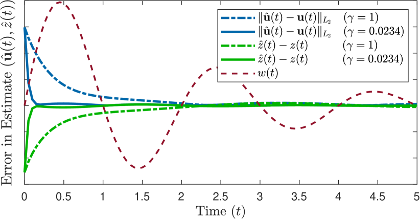
(a) $r=4$

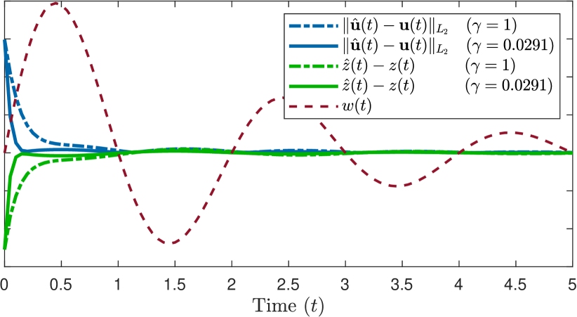
(b) $r=8$

Figure 1: Error in the estimate of the PDE state $\mathbf{u}(t)$ and the output $z(t)$ for the PDE in Subsection 5.1 with $r=4$ and $r=8$, for disturbance $w(t)=5e^{-t}\sin(t)$ and initial error $\hat{\mathbf{u}}(0,x,y)-\mathbf{u}(0,x,y)=2((x-1)^{4}-1)\sin(0.5\pi y)$. Errors are plotted for estimators achieved both for fixed $\gamma=1$ in the LMI in Cor. 12, as well as minimizing over the value of $\gamma$ in this LMI.

We consider the following 2D heat equation, with sensors along the upper boundary,

$$\mathbf{u}_{t}(t) =\mathbf{u}_{xx}(t)+\mathbf{u}_{yy}(t)+r\mathbf{u}(t)+w(t),$$

$$z(t) =\int_{0}^{1}\int_{0}^{1}\mathbf{u}(t,x,y)dxdy,$$

$$\mathbf{q}_{1}(t) =\mathbf{u}(t,1,\cdot),\quad\mathbf{q}_{2}(t)=\mathbf{u}(t,\cdot,1),$$

$$\mathbf{u}(t,0,\cdot) =\mathbf{u}_{x}(t,1,\cdot)\equiv 0,\quad\mathbf{u}(t,\cdot,0)=\mathbf{u}_{y}(t,\cdot,1)\equiv 0,$$

where $\mathbf{u}(t)\in L_{2}[[0,1]^{2}]$, $w(t),z(t)\in\mathbb{R}$, and $\mathbf{q}(t)=\left[\scriptsize\begin{smallmatrix}\mathbf{q}_{1}(t)\\ \mathbf{q}_{2}(t)\end{smallmatrix}\right]\in L_{2}^{2}[0,1]$. Using PIETOOLS, we construct a PIE representation associated to this system and synthesize an estimator for values of the parameter $r=4$ and $r=8$, for which the system is stable and unstable, respectively. Minimizing the variable $\gamma$ in Cor. 12, we obtain optimal gain operators $\mathcal{L}$ that achieve lowest bounds on the $H_{\infty}$-norm of the associated error dynamics as $\gamma=0.0234$ and $\gamma=0.0291$ for $r=4$ and $r=8$, respectively. In addition, for each value of $r\in\{4,8\}$, sub-optimal gains $\mathcal{L}$ were also computed for a fixed bound $\gamma=1$ in the LMI.

The error dynamics corresponding to the obtained estimators were simulated with disturbance $w(t)=5e^{-t/2}\sin(\pi t)$ and initial state $\mathbf{u}_{0}(t,x,y)=5((x-1)^{4}-1)\sin(0.5\pi y)$, starting with an initial state estimate $\hat{\mathbf{u}}(0)=0$. Figure 1 shows the norm of the error in the PDE state and output for $t\in[0,5]$, as well as the value of the disturbance. The plots show that, both for the stable ($r=4$) and unstable ($r=8$) PDE, the error in the estimates of the state and output converge to zero, with faster convergence achieved using the optimal estimators associated to the minimized bounds $\gamma$.

6 Conclusion

In this paper, a new convex-optimization-based method was presented for estimator synthesis of linear, 2nd order, 2D PDEs with state observations along the boundary. To this end, it was proved that any sufficiently well-posed such PDE can be equivalently represented as a PIE, specifically proving that the value of the state $\mathbf{u}$ along the boundary can be expressed in terms of a PI operator acting on the fundamental state $\partial_{x}^{2}\partial_{y}^{2}\mathbf{u}$. Parameterizing a Luenberger-type estimator for the PIE by a PI operator, it was then shown that a value of this operator with guaranteed bound on the $H_{\infty}$-norm of the estimator error dynamics can be computed by solving an LPI, which in turn could be solved as an LMI. The proposed methodology has been incorporated in the PIETOOLS software suite, and applied to construct an estimator for an unstable heat equation, using simulation to show convergence of the estimated state to the true value.

Appendix A Numerical Simulation of PIEs

In section 5, we applied the proposed LPi methodology to construct an estimator for a 2D heat equation with state observations along the boundary. To test the performance of this estimator, we simulated the dynamics of the associated error $\mathbf{e}(t)=\mathbf{v}(t)-\hat{\mathbf{v}}(t)$ in the fundamental state $\mathbf{v}(t)=\partial_{x}^{2}\partial_{y}^{2}\mathbf{u}(t)$, defined by the PIE (20). In particular, we model this error using a Galerkin approach, wherein we consider the error state $\mathbf{e}(t)$ only on a finite-dimensional subspace $Y\subseteq L_{2}[[0,1]]$, spanned by a basis of pairwise orthonormal functions $\boldsymbol{\phi}_{i}\in L_{2}[[0,1]^{2}]$ for $i\in\{1,\ldots,N\}$, so that $\left\langle\boldsymbol{\phi}_{i},\boldsymbol{\phi}_{j}\right\rangle_{L_{2}}=1$ if $i=j$ but $0$ otherwise. Then, the error at any time is defined by a vector of coefficients $c_{k}(t)\in\mathbb{R}^{N}$ as $\mathbf{e}(t)=\sum_{j=1}^{N}c_{j}(t)\boldsymbol{\phi}_{j}$, and we can express

$$\mathcal{T}\mathbf{e}_{t}(t)=\sum_{j=1}^{N}\dot{c}_{j}(t)(\mathcal{T}\boldsymbol{\phi}_{j}),\qquad\bar{\mathcal{A}}\mathbf{e}(t)=\sum_{j=1}^{N}c_{j}(t)(\bar{\mathcal{A}}\boldsymbol{\phi}_{j}).$$

We require this error to weakly satisfy the PIE (21) on the space $Y$, so that

$$\left\langle\boldsymbol{\phi}_{i},\mathcal{T}\mathbf{e}_{t}(t)\right\rangle_{L_{2}}=\left\langle\boldsymbol{\phi}_{i},\bar{\mathcal{A}}\mathbf{e}(t)+\bar{\mathcal{B}}w(t)\right\rangle,\quad\forall i\in\{1,\ldots,N\}.$$

Defining matrices $T,\bar{A}\in\mathbb{R}^{N\times N}$ by $T_{ij}:=\left\langle\boldsymbol{\phi}_{i},\mathcal{T}\boldsymbol{\phi}_{j}\right\rangle_{L_{2}}$ and $\bar{A}_{ij}:=\left\langle\boldsymbol{\phi}_{i},\bar{\mathcal{A}}\boldsymbol{\phi}_{j}\right\rangle_{L_{2}}$, the resulting system can then be represented as an ODE on the vector of coefficients $c(t)\in\mathbb{R}^{N}$

$$T\dot{c}(t)=Ac(t)+\left\langle\boldsymbol{\phi},\mathcal{B}w(t)\right\rangle_{L_{2}}.$$

Assuming the matrix $T$ to be invertible, this system can be numerically solved for a given input $w$ using any time-stepping scheme, starting with an initial value of the coefficients as $c_{j}(0)=\left\langle\boldsymbol{\phi}_{j},\mathbf{e}(0)\right\rangle_{L_{2}}=\left\langle\boldsymbol{\phi}_{j},\partial_{x}^{2}\partial_{y}^{2}\hat{\mathbf{u}}(0)-\partial_{x}^{2}\partial_{y}^{2}\mathbf{u}(0)\right\rangle_{L_{2}}$. From the obtained values of the coefficients at each time, the error in the estimate of the fundamental state can then be computed as $\mathbf{e}(t)=\sum_{j=1}^{N}c_{j}(t)\boldsymbol{\phi}_{j}$, and we can retrieve the error in the estimate of the PDE state as $\mathcal{T}\mathbf{e}(t)=\sum_{j=1}^{N}c_{j}(t)\mathcal{T}\boldsymbol{\phi}_{j}$. The error $\hat{z}(t)$ in the regulated output can then be computed directly from the PIE (21).

For the numerical implementation in Section 5, the basis functions $\boldsymbol{\phi}_{i}$ were chosen as Legendre polynomials of degree at most $4$ in each variable $x,y\in[0,1]$, yielding a total of $N=(4+1)^{2}=25$ basis functions. For the numerical time-stepping, an explicit Euler scheme was applied as

$$c(t_{k+1})=c(t_{k})+\Delta t(T^{-1}Ac(t_{k})+\left\langle\boldsymbol{\phi},\mathcal{B}w(t)\right\rangle_{L_{2}})$$

using a time step $\Delta t=10^{-3}$, and simulating from $t_{0}=0$ up to $t_{N_{t}}=10$.