Connecting Kani’s Lemma and path-finding in the Bruhat-Tits tree to compute supersingular endomorphism rings

Abstract.

We give a deterministic polynomial time algorithm to compute the endomorphism ring of a supersingular elliptic curve in characteristic $p$, provided that we are given two noncommuting endomorphisms and the factorization of the discriminant of the ring $\mathcal{O}_{0}$ they generate. At each prime $q$ for which $\mathcal{O}_{0}$ is not maximal, we compute the endomorphism ring locally by computing a $q$-maximal order containing it and, when $q\neq p$, recovering a path to $\text{End}(E)\otimes\mathbb{Z}_{q}$ in the Bruhat-Tits tree. We use techniques of higher-dimensional isogenies to navigate towards the local endomorphism ring. Our algorithm improves on a previous algorithm which requires a restricted input and runs in subexponential time under certain heuristics. Page and Wesolowski give a probabilistic polynomial time algorithm to compute the endomorphism ring on input of a single non-scalar endomorphism. Beyond using techniques of higher-dimensional isogenies to divide endomorphisms by a scalar, our methods are completely different.

1. Introduction

One of the fundamental problems in computational arithmetic geometry is computing the endomorphism ring of an elliptic curve. In the ordinary case, Bisson and Sutherland [BS11] gave a subexponential time algorithm for this problem under certain heuristics, later improved to rely only on GRH [Bis12]. Recently, Robert outlined an algorithm to compute the endomorphism ring of an ordinary elliptic curve in polynomial time, assuming access to a factoring oracle [Rob23b, Theorem 4.2].

In this paper we give a deterministic polynomial time algorithm that computes the endomorphism ring of a supersingular elliptic curve, given two non-commuting endomorphisms and a factorization of the reduced discriminant of the order they generate. Beside being of intrinsic interest, computing the endomorphism ring of a supersingular elliptic curve has become a central problem in isogeny-based cryptography. The first cryptographic application of isogenies between supersingular elliptic curves was the hash function in [CGL09]. The security of this hash function depends on the hardness of computing endomorphism rings. More generally, the hardness of computing endomorphism rings is necessary for the security of all isogeny-based cryptosystems [EHL⁺18, Wes21, Wes22].

Computing the endomorphism ring of a supersingular elliptic curve $E$ was first studied by Kohel [Koh96, Theorem 75], who gave an approach for generating a subring of finite index of the endomorphism ring $\text{End}(E)$. The algorithm is based on finding cycles in the $\ell$-isogeny graph of supersingular elliptic curves in characteristic $p$ and runs in time $O(p^{1+\varepsilon})$. In this paper we complete Kohel’s approach by showing how to compute $\text{End}(E)$ from a suborder. This builds on [EHL⁺20] which gave a subexponential algorithm, under certain heuristics, if the input suborder was Bass. In [FIK⁺23], it is shown that under GRH, a Bass suborder of $\text{End}(E)$ can be computed in $O(p^{1/2+\varepsilon})$ time. In a different direction, one can attempt to compute $\text{End}(E)$ by constructing a generating set. In [GPS17] it is argued that heuristically one expects $O(\log p)$ calls to a cycle finding algorithm until the cycles generate $\text{End}(E)$. Under different heuristics, [FIK⁺23] argues that a basis for $\text{End}(E)$ can be found in $O(1)$ applications to an algorithm to produce inseparable endomorphisms. An algorithm for computing powersmooth endomorphisms with complexity $\tilde{O}(p^{1/2})$ and polynomial storage is given by Delfs and Galbraith [DG16]. Page and Wesolowski give an unconditional probabilistic polynomial-time algorithm for the computation of the full endomorphism ring whose complexity is also $\tilde{O}(p^{1/2})$ [PW23].

One of the main proposals in isogeny-based cryptography, SIDH, was broken in July 2022 [CD23, MMP⁺23, Rob23a]. In SIDH, the underlying hard problem is finding paths in the isogeny graph when certain torsion-point information is revealed. The groundbreaking idea for the break of SIDH relied on moving this problem into a more flexible framework using isogenies between products of elliptic curves, via Kani’s Lemma. We apply these techniques to the more general problem of computing supersingular endomorphism rings. There are other recent papers which have also exploited higher-dimensional isogenies, such as the new post-quantum signature scheme SQIsignHD [DLRW23]. They are also used to answer the question of how much knowing one non-scalar endomorphism helps in computing the full endomorphism ring [HLMW23, PW23]. In [PW23], it is shown that computing the endomorphism ring of a supersingular elliptic curve is equivalent under probabilistic polynomial time reductions to the problem of computing a single non-scalar endomorphism.

Our algorithm is an improvement and a generalization of the main result in [EHL⁺20], which we summarize briefly here. Given a Bass order $\mathcal{O}_{0}$ and a factorization of the reduced discriminant $\operatorname{discrd}(\mathcal{O}_{0})$, they compute all local maximal orders containing $\mathcal{O}_{0}\otimes\mathbb{Z}_{q}$ at each prime $q$ dividing $\operatorname{discrd}(\mathcal{O}_{0})$. They then combine the local information to obtain all global maximal orders $\mathcal{O}$ containing $\mathcal{O}_{0}$ and check if each maximal order $\mathcal{O}$ is isomorphic to $\text{End}(E)$. The Bass restriction on $\mathcal{O}_{0}$ is needed to bound the number of maximal orders.

Our algorithm also approaches the problem locally. However, we are able to determine the local maximal order $\text{End}(E)\otimes\mathbb{Z}_{q}$ without constructing global candidates for $\text{End}(E)$. We also do not require the Bass restriction, although we can give a more efficient algorithm when $\mathcal{O}_{0}$ is Bass.

There are two key tools. The first is a polynomial-time algorithm which, when given an endomorphism $\beta$ and an integer $n$, determines if $\frac{\beta}{n}$ is an endomorphism. This algorithm is implicit in Robert’s algorithm for computing an endomorphism ring of an ordinary elliptic curve [Rob23b, Section 4]. A detailed proof and runtime analysis are given in [HLMW23, Section 4]. It is also used in [PW23] to compute the endomorphism ring on input of a non-scalar endomorphism. Given a non-scalar endomorphism, they randomly sample endomorphisms to generate an order with certain properties and apply this algorithm to recover the full endomorphism ring. In contrast, our deterministic algorithm applies this algorithm to locate $\text{End}(E)\otimes\mathbb{Z}_{q}$ in the subtree of the Bruhat-Tits tree that contains a given suborder, without needing to enlarge our input order.

The second is a theorem by Tu which expresses an intersection of finitely many maximal orders in $M_{2}(\mathbb{Q}_{q})$ as an intersection of at most three maximal orders, which can be constructed explicitly. Together with the containment testing, this allows us to rule out many local maximal orders at once and find $\text{End}(E)\otimes\mathbb{Z}_{q}$.

In the general case, our algorithm works as follows. At each prime $q$ dividing the reduced discriminant, we construct a global order $\tilde{\mathcal{O}}$ containing $\mathcal{O}_{0}$ which is maximal at $q$ and is equal to $\mathcal{O}_{0}\otimes\mathbb{Z}_{q^{\prime}}$ at all other primes $q^{\prime}$. If $q\neq p$, then $\tilde{\mathcal{O}}\otimes\mathbb{Z}_{q}$ may not be equal to $\text{End}(E)\otimes\mathbb{Z}_{q}$, but it is conjugate via an element of $M_{2}(\mathbb{Z}_{q})$ which our algorithm constructs explicitly, step-by-step. Given the valuation $e=v_{q}(\operatorname{discrd}(\mathcal{O}_{0}))$, we are able to recover the correct matrix with at most $4(eq+2)$ applications of Proposition 2.4. In the case that $\mathcal{O}_{0}$ is Bass at $q$, in which case there are at most $e+1$ choices, we are able to recover the correct matrix with $4\log_{2}(e+1)$ applications of Proposition 2.4.

Theorem 1.1.

There exists an algorithm that computes the endomorphism ring of a supersingular elliptic curve $E$ when given $E$, two noncommuting endomorphisms $\alpha$ and $\gamma$ which can be evaluated efficiently on powersmooth torsion points, and a factorization of the reduced discriminant $\Delta$ of the order generated by $\alpha$ and $\gamma$. The algorithm runs in polynomial time in $\log p$, the size of $\alpha$ and $\gamma$, $\log\Delta$, and is linear in the number of primes dividing $\Delta$ and the largest prime dividing $\Delta$.

This paper is organized as follows. In Section 2, we give some background on isogenies and quaternion algebras. In Section 3, we review the Bruhat-Tits tree and results on intersections of finitely many maximal orders. We work with an order $\mathcal{O}_{0}$ that has finite index in the endomorphism ring $\text{End}(E)$. In Section 4, we take a maximal local order containing the starting order $\mathcal{O}_{0}\otimes\mathbb{Z}_{q}$ and compute its distance from $\text{End}(E)\otimes\mathbb{Z}_{q}$ in the Bruhat-Tits tree (Algorithm 4.5). In Section 5, we give an algorithm to test whether an

$\text{End}(E)\otimes\mathbb{Z}_{q}$. This is used in Section 6, to find a path from our starting local maximal order to $\text{End}(E)\otimes\mathbb{Z}_{q}$. In Section 7, we give a more efficient algorithm in the Bass case. Finally in Section 8, we put everything together and give the algorithm for computing the full endomorphism ring from our starting order $\mathcal{O}_{0}$.

2. Preliminaries and Definitions

2.1. Orders and Lattices in Quaternion Algebras, Discriminants

Definition 2.1.

Let $R$ be a domain with field of fractions $F$, and let $B$ be a finite-dimensional $F$-algebra. A subset $M\subseteq V$ is an $R$-lattice if $M$ is finitely generated as an $R$-module and $MF=B$. An $R$-order $\mathcal{O}\subseteq B$ is an $R$-lattice that is also a subring of $B$. An order is maximal if it is not properly contained in another order.

Definition 2.2.

Let $F$ be $\mathbb{Q}$ or $\mathbb{Q}_{q}$ (with $q>2$). For $a,b\in F^{\times}$, let $H(a,b)$ denote the quaternion algebra over $F$ with basis $1,i,j,ij$ such that $i^{2}=a$, $j^{2}=b$ and $ij=-ji$. That is, $H(a,b)=\mathbb{Q}+\mathbb{Q}\,i+\mathbb{Q}\,j+\mathbb{Q}\,ij.$

Any quaternion algebra over $F$ can be written in this form. For the case of $F=\mathbb{Q}_{2}$, see [Voi21, Section 6.2].

There is a standard involution on $H(a,b)$ which maps $\alpha~{}=~{}a_{1}+a_{2}i+a_{3}j+a_{4}ij$ to $\overline{\alpha}:=a_{1}-a_{2}i-a_{3}j-a_{4}ij$. The reduced trace of such an element $\alpha$ is defined as $\operatorname{Trd}(\alpha)=\alpha+\overline{\alpha}=2a_{1},$. The reduced norm is $\operatorname{Nrd}(\alpha)=\alpha\overline{\alpha}=a_{1}^{2}-aa_{2}^{2}-ba_{3}^{2}+aba_{4}^{2}.$

We say that a quaternion algebra $B$ over $\mathbb{Q}$ ramifies at a prime $q$ (respectively $\infty$) if $B\otimes\mathbb{Q}_{q}$ (respectively $B\otimes\mathbb{R}$) is a division algebra. Otherwise, $B$ is said to be split at $q$. In this case, $B\otimes\mathbb{Q}_{q}\cong M_{2}(\mathbb{Q}_{q})$.

The discriminant of a quaternion algebra $B$, denoted $\operatorname{disc}B$, is the product of primes that ramify in $B$. For an order $\mathcal{O}\subset B$ with $\mathbb{Z}$-basis $\{\alpha_{1},\alpha_{2},\alpha_{3},\alpha_{4}\}$, the discriminant of $\mathcal{O}$ is defined to be $\operatorname{disc}(\mathcal{O})\coloneqq|\det(\operatorname{Trd}(\alpha_{i}\alpha_{j}))_{i,j}|\in\mathbb{Z}>0$ [Voi21, p. 242]. The discriminant of an order is always a square. The reduced discriminant $\operatorname{discrd}(\mathcal{O})$ is the positive integer square root of $\operatorname{disc}(\mathcal{O})$  [Voi21, p. 242].

For a supersingular elliptic curve $E$ defined over a finite field of characteristic $p$, the endomorphism ring $\text{End}(E)$ is a maximal order of the quaternion algebra $B_{p,\infty}$, the unique quaternion algebra ramified at the primes $p$ and $\infty$. For this paper, computing the endomorphism ring $\text{End}(E)$ means producing a basis of endomorphisms which can be evaluated at powersmooth torsion points and generate $\text{End}(E)$.

One key fact that we will need to enlarge the given order $\mathcal{O}_{0}$ to $\text{End}(E)$, a maximal order in $B_{p,\infty}$, is the local-global principle. This states that an order in a global quaternion algebra is determined by its completions at each prime, see [Voi21, Theorem 9.4.9, Lemma 9.5.3]. We use the fact that maximality is a local property, i.e. an order $\mathcal{O}\subseteq B_{p,\infty}$ is maximal if and only if for all primes $q$, $\mathcal{O}\otimes\mathbb{Z}_{q}$ is a maximal order. Being maximal can also be expressed in terms of the reduced discriminant: an order $\mathcal{O}$ in $B_{p,\infty}$ is maximal if and only if the reduced discriminant $\operatorname{discrd}(\mathcal{O})$ is equal to $p$ [Voi21, p. 375]. The primes at which $\mathcal{O}$ fails to be maximal are exactly those primes dividing $\operatorname{discrd}(\mathcal{O})/p$.

Thus, the local-global principle reduces finding $\text{End}(E)$ to finding $\text{End}(E)\otimes\mathbb{Z}_{q}$ at each prime $q$ dividing $\operatorname{discrd}(\mathcal{O})/p$. When $q=p$, there is a unique maximal order in the division algebra $B_{p,\infty}\otimes\mathbb{Z}_{p}$. In the case that $q\neq p$, the local order $\text{End}(E)\otimes\mathbb{Z}_{q}$ is a maximal order of $B_{p,\infty}\otimes\mathbb{Q}_{q}\cong M_{2}(\mathbb{Q}_{q})$.

Definition 2.3.

Let $\mathcal{O}_{0}$ be an order. We say that an order $\mathcal{O}$ is a $q$-enlargement of $\mathcal{O}_{0}$ if $\mathcal{O}_{0}\subset\mathcal{O}$ and $\mathcal{O}\otimes\mathbb{Z}_{q^{\prime}}=\mathcal{O}_{0}\otimes\mathbb{Z}_{q^{\prime}}$ for all $q^{\prime}\neq q$. We say that $\mathcal{O}$ is a $q$-maximal $q$-enlargement if $\mathcal{O}$ is a q-enlargement such that $\mathcal{O}\otimes\mathbb{Z}_{q}$ is maximal.

Let $\mathcal{O}\subset B$ be a $\mathbb{Z}$-order. We call $\mathcal{O}$ an Eichler order if $\mathcal{O}\subseteq B$ is the intersection of two (not necessarily distinct) maximal orders. The codifferent of an order is $\operatorname{codiff}(\mathcal{O)}=\{\alpha\in B:\operatorname{Trd}(\alpha\mathcal{O})\subseteq\mathbb{Z}\}.$ We say that $\mathcal{O}$ is Gorenstein if the lattice codiff$(\mathcal{O})$ is invertible as a lattice [Voi21, 24.1.1]. We call $\mathcal{O}$ Bass if every superorder $\mathcal{O}^{\prime}\supseteq\mathcal{O}$ is Gorenstein.

One of the key tools we will use is an algorithm which determines if a rational multiple of an endomorphism is an endomorphism.

Proposition 2.4.

[Divide algorithm] There exists an algorithm which takes as input an elliptic curve $E$ defined over $\mathbb{F}_{p^{k}}$, an endomorphism $\beta\in\text{End}(E)$, and an integer $n$, and outputs TRUE if $\frac{\beta}{n}\in\text{End}(E)$ and FALSE if $\frac{\beta}{n}\not\in\text{End}(E)$. The algorithm runs in polynomial-time in $\log(p^{k})$ and $\log(\deg(\beta))$.

This algorithm was first outlined by Robert in a special case to compute endomorphism rings of ordinary curves [Rob23b, Section 4]. The main idea is to use Kani’s Lemma to translate the problem into a higher dimension, where there is enough flexibility to impose powersmoothness. A proof of Proposition 2.4 is given in [HLMW23, Section 4]. Before [HLMW23] was posted, we had written down the details for the algorithm, proof of correctness, and run-time analysis, which we include in Appendix A. We will refer to this algorithm by our original name for it, the Endomorphism-Testing Algorithm.

3. Local Orders and the Bruhat-Tits Tree

Given an order $\mathcal{O}_{0}$ of finite index in $\text{End}(E)$, we will compute $\text{End}(E)$ from $\mathcal{O}_{0}$ by enlarging it so that locally at a prime $q$ it is maximal and equal to $\text{End}(E)\otimes\mathbb{Z}_{q}$. When $q=p$ this step follows from work done in [Voi13] since $B_{p,\infty}\otimes\mathbb{Z}_{p}$ is a division algebra and has a unique maximal order. When $q\neq p$ we will first compute some maximal order containing $\mathcal{O}_{0}\otimes\mathbb{Z}_{q}$ and then find a path from that maximal order to $\text{End}(E)\otimes\mathbb{Z}_{q}$. Here we view both orders as vertices in the Bruhat-Tits tree for $GL_{2}(\mathbb{Q}_{q})$.

Remark 3.1.

Throughout this paper, a path in the Bruhat-Tits tree always refers to a nonbacktracking path.

3.1. Bruhat-Tits tree

For the remainder of this section, fix a prime $q\neq p$. We use the labelling conventions described by Tu [Tu11].

Definition 3.2.

The Bruhat-Tits tree is the graph whose vertices are rank 2 $\mathbb{Z}_{q}$-lattices up to homothety. Two lattice classes $[L]$ and $[L^{\prime}]$ are connected by an edge if and only if there are representatives $L$ and $L^{\prime}$ such that $qL^{\prime}\subsetneq L\subsetneq L^{\prime}$.

Equivalently, one can consider the vertices of the Bruhat-Tits tree as maximal orders of $M_{2}(\mathbb{Q}_{q})$, via the correspondence $[L]\mapsto\text{End}(L)$. In this case, two maximal orders $\Lambda$ and $\Lambda^{\prime}$ are neighbors if and only if $[\Lambda:\Lambda\cap\Lambda^{\prime}]=[\Lambda^{\prime}:\Lambda\cap\Lambda^{\prime}]=q$.

Fixing a basis for a lattice $L_{0}$ and identifying $\text{End}(L_{0})$ with $M_{2}(\mathbb{Z}_{q})$, we associate to each basis defining a lattice $L$ a $2\times 2$ matrix $T$ that transforms the basis of $L$ into that of $L_{0}$.

Then $\text{End}(L)=T^{-1}M_{2}(\mathbb{Z}_{q})T.$ Given $L_{0}$ and $L$, the matrix $T$ is well-defined as an element of $\mathbb{Q}_{q}^{*}\operatorname{GL}_{2}(\mathbb{Z}_{q})\backslash\operatorname{GL}_{2}(\mathbb{Q}_{q})$, so we may assume that $T$ is of the form $T=\begin{pmatrix}q^{a}&c\\ 0&q^{b}\\ \end{pmatrix}$ with $a,b\geq 0$, $c\in\mathbb{Z}/q^{b}\mathbb{Z}$, and $v_{q}(c)=0$ if both $a$ and $b$ are positive.

The Bruhat-Tits tree is a $(q+1)$-regular tree. Each neighbor of a lattice $L$ corresponds to a choice of cyclic sublattice of order $q$, which corresponds to a choice of matrices of the form $\begin{pmatrix}q&c\\ 0&1\end{pmatrix}$ and $\begin{pmatrix}1&0\\ 0&q\end{pmatrix}$. More generally, a path of length $n$ starting at the root $M_{2}(\mathbb{Z}_{q})$ (labelled by the $2\times 2$ identity matrix) corresponds to a product of such matrices. We make the following definition.

Definition 3.3.

For each $c$ such that $0\leq c\leq q-1$, let $\gamma_{c}:=\begin{pmatrix}1&c\\ 0&q\end{pmatrix}$. Let $\gamma_{\infty}=\begin{pmatrix}q&0\\ 0&1\end{pmatrix}$. Let $\Sigma=\{\gamma_{c}:0\leq c\leq q-1\}\cup\{\gamma_{\infty}\}$. We call a finite sequence of matrices $\{c_{i}\}_{i=1}^{n}$ a matrix path if each $c_{i}\in\Sigma$ and $c_{i+1}c_{i}\not\in qM_{2}(\mathbb{Z}_{q})$. The length of the matrix path $\{c_{i}\}_{i=1}^{n}$ is $n$. Each path of length $n$ starting at the root corresponds to a matrix path. If $\{c_{i}\}_{i=1}^{n}$ is a matrix path, we call the product $T=c_{n}c_{n-1}\ldots c_{1}$ the associated matrix.

There is a bijection between paths of length $n$ in the Bruhat-Tits tree starting at $M_{2}(\mathbb{Z}_{q})$ and matrix paths of length $n$. The endpoint of the path corresponding to the matrix path $\{c_{i}\}_{i=1}^{n}$ is the order $T^{-1}M_{2}(\mathbb{Z}_{q})T$, where $T$ is the associated matrix. The vertices of the path are

$$M_{2}(\mathbb{Z}_{q}),c_{1}^{-1}M_{2}(\mathbb{Z}_{q})c_{1},c_{1}^{-1}c_{2}^{-1}M_{2}(\mathbb{Z}_{q})c_{2}c_{1},\ldots,(c_{1}^{-1}c_{2}^{-1}\cdots c_{n}^{-1})M_{2}(\mathbb{Z}_{q})(c_{n}\cdots c_{2}c_{1}).$$

Depending on the context, we may represent vertices in the Bruhat-Tits tree as maximal orders in $M_{2}(\mathbb{Z}_{q})$, lattices, or $2\times 2$ matrices $T$ as above.

3.2. Distance

We have the usual notion of distance in the Bruhat-Tits tree.

Definition 3.4.

The distance between two vertices in the Bruhat-Tits tree $v$ and $v^{\prime}$, denoted $d(v,v^{\prime})$, is the length of the unique path between $v$ and $v^{\prime}$. We denote the distance between $v$ and $v^{\prime}$ by $d(v,v^{\prime})$. Here, $v$ and $v^{\prime}$ may be represented by homothety classes of lattices, maximal orders in $M_{2}(\mathbb{Z}_{q})$, or the matrices associated to the matrix path.

Definition 3.5.

Let $\ell$ be a postive integer and $v$ a vertex in the Bruhat-Tits tree. The $\ell$-neighborhood of $v$ is the set

$$N_{\ell}(v)\colon=\{v^{\prime}:d(v^{\prime},v)\leq\ell\}.$$

We also have the analogous notion of distance to a path and neighborhood of a path.

Definition 3.6.

Let $P$ be the set of vertices along a path in the Bruhat-Tits tree. The distance between a vertex $v$ and $P$ is $\min\{d(v,v^{\prime})\colon v^{\prime}\in P\}$. The distance between $v$ and $P$ is denoted $d(v,P)$.

Definition 3.7.

Let $P$ be the set of vertices along a path in the Bruhat-Tits tree and let $\ell$ be a nonnegative integer. The $\ell$-neighborhood of $P$ is the set

$$N_{\ell}(P)\colon=\{v^{\prime}:d(v^{\prime},P)\leq\ell\}.$$

3.3. Distance and matrix labelling

This section relates the distance between two vertices in the Bruhat-Tits tree to the matrix labelling just described. We will also get a bound on the distance in terms of the reduced discriminant of the intersection of the two maximal orders.

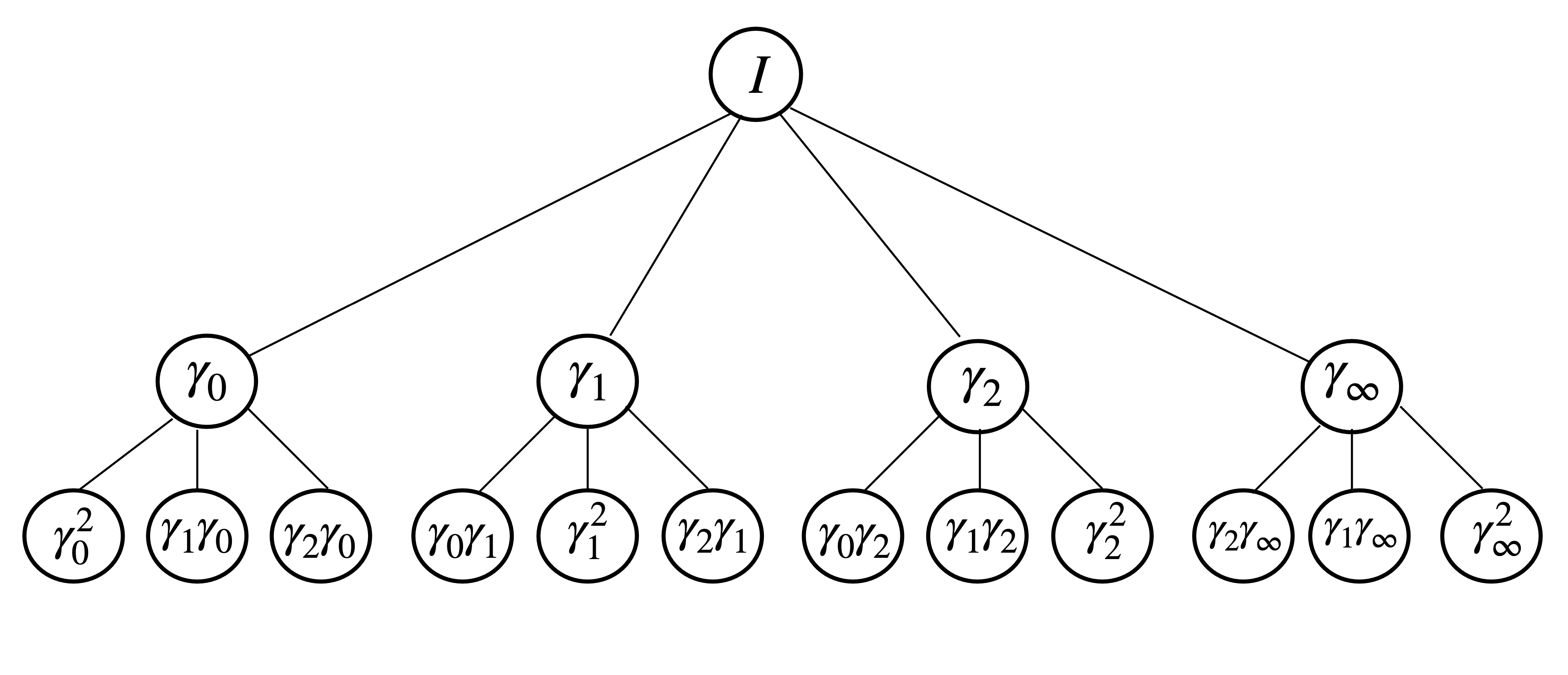
Figure 1. The (truncated) Bruhat-Tits tree for $q=3$, with vertices labelled by the corresponding matrices. The root of the tree, labelled $I$, corresponds to $M_{2}(\mathbb{Z}_{q})$. The vertex labelled with matrix $T$ corresponds to the order $T^{-1}M_{2}(\mathbb{Z}_{q})T.$

Proposition 3.8.

Let $T=b_{r}\cdots b_{2}b_{1}a_{k}\cdots a_{2}a_{1}$ and $T^{\prime}=c_{s}\cdots c_{1}a_{k}\cdots a_{2}a_{1}$, such that $a_{i},b_{i},c_{i}\in\Sigma$, the product of two consecutive matrices is not in $M_{2}(q\mathbb{Z}_{q})$, and $b_{1}\neq c_{1}$. Then

$$d(T^{-1}M_{2}(\mathbb{Z}_{q})T,T^{\prime-1}M_{2}(\mathbb{Z}_{q})T^{\prime})=r+s.$$

Proof.

Let $\gamma=a_{k}\cdots a_{1}.$ The unique path from $T^{-1}M_{2}(\mathbb{Z}_{q})T$ to $M_{2}(\mathbb{Z}_{q})$ and the unique path from $T^{\prime-1}M_{2}(\mathbb{Z}_{q})T^{\prime}$ intersect exactly in the path from $\gamma^{-1}M_{2}(\mathbb{Z}_{q})\gamma$ to $M_{2}(\mathbb{Z}_{q}).$ Thus, we obtain a (nonbacktracking) path from $T^{-1}M_{2}(\mathbb{Z}_{q})T$ to $T^{\prime-1}M_{2}(\mathbb{Z}_{q})T^{\prime}$ by first taking the path of length $r$ from $T^{-1}M_{2}(\mathbb{Z}_{q})T$ to $\gamma^{-1}M_{2}(\mathbb{Z}_{q})\gamma$, and concatenating it with the path of length $s$ from $\gamma^{-1}M_{2}(\mathbb{Z}_{q})\gamma$ to $T^{\prime-1}M_{2}(\mathbb{Z}_{q})T^{\prime}$. ∎

We can relate the reduced discriminant of an order to the distance between maximal orders containing it.

Lemma 3.9.

Let $\Lambda$ be a $\mathbb{Z}_{q}$-order in $M_{2}(\mathbb{Q}_{q})$ such that $\Lambda\subset\Lambda_{1}\cap\Lambda_{2}$ for maximal orders $\Lambda_{1},\Lambda_{2}$. Then $v_{q}(\operatorname{discrd}(\Lambda))\geq v_{q}(\operatorname{discrd}(\Lambda_{1}\cap\Lambda_{2})).$

Proof.

By [Voi21, Lemma 15.2.15], $\operatorname{discrd}(\Lambda)=[\Lambda_{1}\cap\Lambda_{2}:\Lambda]\operatorname{discrd}(\Lambda_{1}\cap\Lambda_{2}).$ The index is an integral ideal, so $v_{q}(\operatorname{discrd}(\Lambda))\geq v_{q}(\operatorname{discrd}(\Lambda_{1}\cap\Lambda_{2})).$ ∎

From the lemma, we obtain the two following useful corollaries.

Corollary 3.10.

Suppose $\Lambda\subset M_{2}(\mathbb{Q}_{q})$ is a $\mathbb{Z}_{q}$-order. Let $e=v_{q}(\operatorname{discrd}(\Lambda)).$ If $\Lambda$ is contained in two maximal orders $\Lambda_{1}$ and $\Lambda_{2}$, then $d(\Lambda_{1},\Lambda_{2})\leq e$.

Proof.

When $\Lambda_{1}$ and $\Lambda_{2}$ are maximal orders, the distance between them is $v_{q}(\operatorname{discrd}(\Lambda_{1}\cap\Lambda_{2}))$. The result then follows from Lemma 3.9. ∎

Corollary 3.11.

Let $\Lambda$ be a $\mathbb{Z}_{q}$-order of finite index in $M_{2}(\mathbb{Q}_{q})$. Then $\Lambda$ is contained in finitely many maximal orders.

Proof.

This is immediate from Corollary 3.10. If $\Lambda_{1}$ is a maximal order containing $\Lambda$, then all maximal orders containing $\Lambda$ are at most $v_{q}(\operatorname{discrd}(\Lambda))$ steps from $\Lambda_{1}$. ∎

Remark 3.12.

Suppose $\Lambda\subset\text{End}(E)\otimes\mathbb{Z}_{q}$. If we can construct a maximal order $\Lambda_{1}$ which contains $\Lambda$, the preceding corollaries give us a starting point for how to locate $\text{End}(E)\otimes\mathbb{Z}_{q}$ in the Bruhat-Tits tree. A naive approach would be to check all orders within $e=v_{q}(\operatorname{discrd}(\Lambda))$ steps from $\Lambda_{1}$ in the Bruhat-Tits tree. However, when $e\geq 1$, there are $1+(q+1)\frac{q^{e}-1}{q-1}$ maximal orders at most $e$ steps from $\Lambda_{1}$. Working with each of these orders is computationally infeasible for general $\Lambda$.

3.4. Finite intersections of maximal orders

In this section, we review Tu’s results on finite intersections of maximal orders in $M_{2}(\mathbb{Q}_{q})$. As an application, for each path $P$ and $\ell\geq 0$, we construct an order $\tilde{\Lambda}$ which is contained in a maximal order $\Lambda^{\prime}$ if and only if $\Lambda^{\prime}\in N_{\ell}(P)$. This construction allows us to work with many maximal orders at once.

We give a definition we will use throughout the paper.

Definition 3.13.

[Tu11, Notation 7] Let $S$ be a finite set of maximal orders. We define

$$d_{3}(S):=\max\{d(\Lambda_{1},\Lambda_{2})+d(\Lambda_{2},\Lambda_{3})+d(\Lambda_{3},\Lambda_{1})\},$$

where the maximum is taken over all choices of $\Lambda_{1},\Lambda_{2},\Lambda_{3}\in S$. The orders $\Lambda_{i}$ need not be distinct.

We restate Tu’s main theorem, specialized to our case $K=\mathbb{Q}_{q}$.

Theorem 3.14.

[Tu11, Theorem 8] Let $S$ be a finite set of maximal orders in $M_{2}(\mathbb{Q}_{q})$. Let $\Lambda_{1},\Lambda_{2},\Lambda_{3}\in S$ be such that $d_{3}(\{\Lambda_{1},\Lambda_{2},\Lambda_{3}\})=d_{3}(S)$. Then $\bigcap_{\Lambda\in S}\Lambda=\Lambda_{1}\cap\Lambda_{2}\cap\Lambda_{3}$. The orders $\Lambda_{1},\Lambda_{2},\Lambda_{3}$ need not be distinct.

Our first lemma relates $d_{3}(S)$ to the reduced discriminant $\operatorname{discrd}(\bigcap_{\Lambda\in S}\Lambda)$.

Lemma 3.15.

Let $S$ be a finite set of maximal orders in $M_{2}{(\mathbb{Q}_{q})}$. Then

$$v_{q}(\operatorname{discrd}(\bigcap_{\Lambda\in S}\Lambda))=d_{3}(S)/2.$$

Proof.

If $S$ consists of a single maximal order $\Lambda_{1}$, then $d_{3}(S)=0$. Furthermore, $\cap_{\Lambda\in S}\Lambda=\Lambda_{1}$ is conjugate to $M_{2}(\mathbb{Z}_{q})$, and therefore $v_{q}(\operatorname{discrd}(\Lambda_{1}))=v_{q}(\operatorname{discrd}(M_{2}(\mathbb{Z}_{q})))=0=d_{3}(S)/2.$

Suppose $\cap_{\Lambda\in S}\Lambda$ is Eichler, say $\cap_{\Lambda\in S}=\Lambda_{1}\cap\Lambda_{2}$ with $\Lambda_{1},\Lambda_{2}\in S$ and such that $d_{3}(S)=d_{3}(\{\Lambda_{1},\Lambda_{2}\})$. Then $v_{q}(\operatorname{discrd}(\Lambda_{1}\cap\Lambda_{2}))=d(\Lambda_{1},\Lambda_{2}).$ Writing $\Lambda_{1}\cap\Lambda_{2}=\Lambda_{1}\cap\Lambda_{2}\cap\Lambda_{2}$, we have $d_{3}(S)=d(\Lambda_{1},\Lambda_{2})+d(\Lambda_{2},\Lambda_{2})+d(\Lambda_{2},\Lambda_{1})=2d(\Lambda_{1},\Lambda_{2}).$ Hence $v_{q}(\operatorname{discrd}(\cap_{\Lambda\in S}\Lambda))=d_{3}(S)/2.$

If $\cap_{\Lambda\in S}\Lambda=\Lambda_{1}\cap\Lambda_{2}\cap\Lambda_{3}$ is not Eichler, let $m=d(\Lambda_{1},\Lambda_{2}),n=d(\Lambda_{2},\Lambda_{3}),\ell=d(\Lambda_{3},\Lambda_{1})$ and assume $m\geq n\geq\ell$. The intersection $\Lambda_{1}\cap\Lambda_{2}\cap\Lambda_{3}$ is conjugate to the order with basis

$$\biggl{\{}\begin{pmatrix}1&0\\ 0&1\end{pmatrix},\begin{pmatrix}0&q^{n}\\ 0&0\end{pmatrix},\begin{pmatrix}0&0\\ q^{m}&0\end{pmatrix},\begin{pmatrix}0&0\\ 0&q^{\ell}\end{pmatrix}\biggl{\}}.$$

(See [Tu11, proof of Theorem 2] for details.)

As $\operatorname{disc}(\{\alpha_{1},\alpha_{2},\alpha_{3},\alpha_{4}\})=\det(\operatorname{Trd}(\alpha_{i}\alpha_{j})),$ a computation shows

$$\operatorname{disc}(\Lambda_{1}\cap\Lambda_{2}\cap\Lambda_{3})=-q^{2m+2n+2\ell}=-q^{d_{3}(S)}.$$

Hence $v_{q}(\operatorname{discrd}(\Lambda_{1}\cap\Lambda_{2}\cap\Lambda_{3}))=d_{3}(S)/2.$ ∎

We’ll also use the following lemma which is key to the proof of Tu’s Theorem 8.

Lemma 3.16.

[Tu11, Lemma 12] Let $S=\{\Lambda_{1},\Lambda_{2},\Lambda_{3}\}$ be a set of maximal orders, and let $\Lambda_{4}$ be a maximal order such that $d_{3}(S\cup\{\Lambda_{4}\})=d_{3}(S).$ Then $\Lambda_{4}\supset\Lambda_{1}\cap\Lambda_{2}\cap\Lambda_{3}.$

The converse is also true, which is shown in the next Lemma.

Lemma 3.17.

Let $S=\{\Lambda_{1},\Lambda_{2},\Lambda_{3}\}$ be a set of maximal orders. Suppose $\Lambda_{4}\supset\Lambda_{1}\cap\Lambda_{2}\cap\Lambda_{3}.$ Then $d_{3}(S)=d_{3}(S\cup\{\Lambda_{4}\}).$

Proof.

We have $v_{q}(\operatorname{discrd}((\bigcap_{\Lambda\in S}\Lambda)\cap\Lambda_{4}))=d_{3}(S\cup\{\Lambda_{4}\})/2,$ and $v_{q}(\operatorname{discrd}(\bigcap_{\Lambda\in S}\Lambda))=d_{3}(S)/2.$ But $\bigcap_{\Lambda\in S}\Lambda\subset\Lambda_{4}$ implies that $(\bigcap_{\Lambda\in S}\Lambda)\cap\Lambda_{4}=\cap_{\Lambda_{\in}S}\Lambda$, hence the reduced discriminants are equal. By Lemma 3.15, $d_{3}(S\cup\{\Lambda_{4}\})=d_{3}(S).$ ∎

Corollary 3.18.

Let $P$ be the set of maximal orders along a path, and let $\ell\geq 0$. Let $\tilde{\Lambda}=\bigcap_{\Lambda\in N_{\ell}(P)}\Lambda$. Then the set of maximal orders containing $\tilde{\Lambda}$ is $N_{\ell}(P)$. Moreover, $v_{q}(\operatorname{discrd}(\tilde{\Lambda}))=3\ell+\operatorname{card}(P)-1$.

Proof.

We will describe $\tilde{\Lambda}$ as an intersection of at most 3 maximal orders.

If $\ell=0$ and $P$ is a single point, then $N_{\ell}(P)$ consists of a single order, which is equal to $\tilde{\Lambda}$. In this case, as $\tilde{\Lambda}$ is maximal, we have $v_{q}(\operatorname{discrd}(\tilde{\Lambda}))=0=\operatorname{card}(P)-1$.

If $\ell=0$ and $\operatorname{card}(P)>1$, then $N_{\ell}(P)=P$. In this case, $\tilde{\Lambda}=\Lambda_{1}\cap\Lambda_{2}$ where $\Lambda_{1}$ and $\Lambda_{2}$ are the endpoints of $P$. The only orders containing $\tilde{\Lambda}$ are those in $P$. We have $v_{q}(\operatorname{discrd}(\Lambda_{1}\cap\Lambda_{2}))=d(\Lambda_{1},\Lambda_{2})=\operatorname{card}(P)-1$.

Now, assume $\ell>0$. Let $\tilde{\Lambda}_{1},\tilde{\Lambda}_{2},\tilde{\Lambda}_{3}$ denote any choice of three orders in $N_{\ell}(P)$, and let $\tilde{\Lambda}_{i}^{\prime}$ denote the order on the path $P$ which is closest to $\tilde{\Lambda}_{i}$.

By the triangle inequality, we have $d(\tilde{\Lambda}_{i},\tilde{\Lambda}_{j})\leq d(\tilde{\Lambda}_{i},\tilde{\Lambda}_{i}^{\prime})+d(\tilde{\Lambda}_{i}^{\prime},\tilde{\Lambda}_{j}^{\prime})+d(\tilde{\Lambda}_{j}^{\prime},\tilde{\Lambda}_{j})\leq 2\ell+d(\tilde{\Lambda}_{i}^{\prime},\tilde{\Lambda}_{j}^{\prime}).$ Hence $d_{3}(\{\tilde{\Lambda}_{1},\tilde{\Lambda}_{2},\tilde{\Lambda}_{3}\})\leq 6\ell+d(\tilde{\Lambda}_{1}^{\prime},\tilde{\Lambda}_{2}^{\prime})+d(\tilde{\Lambda}_{2}^{\prime},\tilde{\Lambda}_{3}^{\prime})+d(\tilde{\Lambda}_{3}^{\prime},\tilde{\Lambda}_{1}^{\prime})$. Since $\tilde{\Lambda}_{1}^{\prime},\tilde{\Lambda}_{2}^{\prime},\tilde{\Lambda}_{3}^{\prime}$ lie along the same path $P$, this sum is at most $2(\operatorname{card}(P)-1)$. Hence $d_{3}(N_{\ell}(P))\leq 6\ell+2(\operatorname{card}(P)-1)$.

Now, choose orders $\Lambda_{i}\in N_{\ell}(P)$ in the following way: Choose a path of length $\ell$ starting at an endpoint $\Lambda_{1}^{\prime}$ of $P$ which is otherwise disjoint from $P$; the end of this path will be $\Lambda_{1}$. To construct $\Lambda_{2}$, choose a path of length $\ell$ which starts at the opposite endpoint $\Lambda_{2}^{\prime}$ of $P$ and is otherwise disjoint from both $P$ and the path from $\Lambda_{1}$ to $\Lambda_{1}^{\prime}$. As the Bruhat-Tits tree is $(q+1)$-regular and $q\geq 2$, this can be done. By construction, $d(\Lambda_{1},\Lambda_{2})=2\ell+\operatorname{card}(P)-1$.

We then construct $\Lambda_{3}$ as follows. Choose a path of length $\ell$ starting at any point of $P$ which is otherwise disjoint from the paths $P$, the path from $\Lambda_{1}$ to $\Lambda_{1}^{\prime}$, and the path from $\Lambda_{2}$ to $\Lambda_{2}^{\prime}$. The path from $\Lambda_{1}$ to $\Lambda_{1}^{\prime}$ and $\Lambda_{2}$ to $\Lambda_{2}^{\prime}$ are automatically disjoint unless $P$ is a single point. Thus, this disjointness restriction can be accomplished if and only if we can choose a path starting at any point of $P$ to avoid two adjacent edges. As the Bruhat-Tits tree is $(q+1)$-regular and $q\geq 2$, we can choose $\Lambda_{1},\Lambda_{2},$ and $\Lambda_{3}$ as specified. By construction, $d(\Lambda_{1},\Lambda_{3})+d(\Lambda_{2},\Lambda_{3})=d(\Lambda_{1},\Lambda_{2})+2\ell=4\ell+2(\operatorname{card}(P)-1)$.

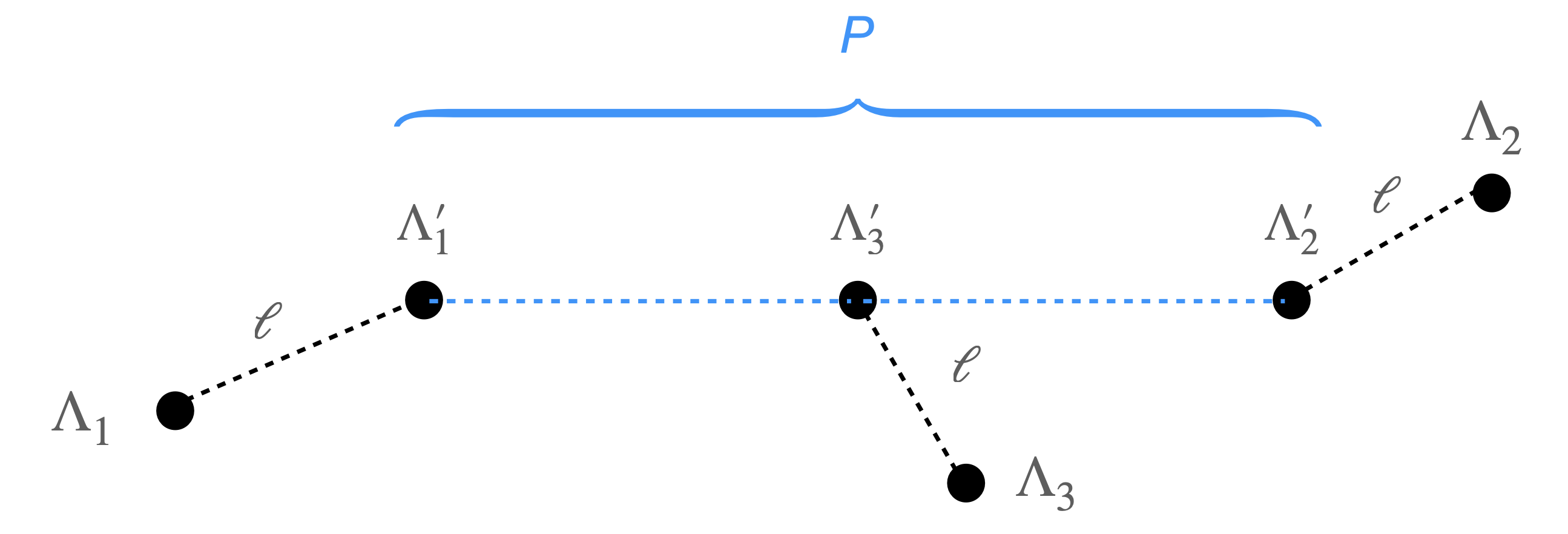
Figure 2. Constructing $\Lambda_{1},\Lambda_{2},\Lambda_{3}$ such that $\bigcap_{\Lambda\in N_{\ell}(P)}\Lambda=\Lambda_{1}\cap\Lambda_{2}\cap\Lambda_{3}.$

For this choice of $\Lambda_{1},\Lambda_{2},\Lambda_{3}$, we have $d_{3}(\{\Lambda_{1},\Lambda_{2},\Lambda_{3}\})=6\ell+2(\operatorname{card}(P)-1)$. Thus, $d_{3}(N_{\ell}(P))=6\ell+2(\operatorname{card}(P)-1)$. By Theorem 3.14, we can write $\tilde{\Lambda}=\Lambda_{1}\cap\Lambda_{2}\cap\Lambda_{3}$, and by Lemma 3.15, we have $v_{q}(\operatorname{discrd}(\tilde{\Lambda}))=3\ell+\operatorname{card}(P)-1$.

Now, we want to show that the set $S:=\{\Lambda\text{ maximal}\colon\tilde{\Lambda}\subset\Lambda\}$ is equal to $N_{\ell}(P)$. It is clear that $N_{\ell}(P)\subset S$ by construction. Suppose $\Lambda_{4}\not\in N_{\ell}(P)$, so that $d(\Lambda_{4},P)>\ell$. We will show that $d_{3}(\{\Lambda_{1},\Lambda_{2},\Lambda_{3},\Lambda_{4}\})>6\ell+2(\operatorname{card}(P)-1)$ and hence $\Lambda_{4}\not\in S$ by Lemma 3.17.

Let $\Lambda_{4}^{\prime}$ be the point of $P$ which is closest to $\Lambda_{4}$. By construction, the paths $\Lambda_{i}$ to $\Lambda_{i}^{\prime}$ for $i\leq 3$ are pairwise disjoint except possibly at $\Lambda_{i}^{\prime}$. Thus, there is at most one $k$ such that the paths $\Lambda_{k}$ to $\Lambda_{k}^{\prime}$ and $\Lambda_{4}$ to $\Lambda_{4}^{\prime}$ intersect in more than one point.

Case 1: There is no such $k$, or $\Lambda_{4}^{\prime}$ is not one of the endpoints of $P$.

Consider $d_{3}(\{\Lambda_{1},\Lambda_{2},\Lambda_{4}\})$. For distinct $i,j\in\{1,2,4\}$, the path between $\Lambda_{i}$ and $\Lambda_{j}$ passes through $\Lambda_{i}^{\prime}$ and $\Lambda_{j}^{\prime}$. We have $d(\Lambda_{i},\Lambda_{j})=d(\Lambda_{i},\Lambda_{i}^{\prime})+d(\Lambda_{i}^{\prime},\Lambda_{j}^{\prime})+d(\Lambda_{j},\Lambda_{j}^{\prime}).$ By construction, $d(\Lambda_{i},\Lambda_{i}^{\prime})=\ell$ if $i\in\{1,2,3\}$, and since $\Lambda_{1}^{\prime}$ and $\Lambda_{2}^{\prime}$ are the endpoints of $P$, we have $d(\Lambda_{1}^{\prime},\Lambda_{2}^{\prime})+d(\Lambda_{2}^{\prime},\Lambda_{4}^{\prime})+d(\Lambda_{4}^{\prime},\Lambda_{1}^{\prime})=\operatorname{card}(P)-1$. Hence $d_{3}(\{\Lambda_{1},\Lambda_{2},\Lambda_{4}\})=4\ell+2(\operatorname{card}(P)-1)+2d(\Lambda_{4},\Lambda_{4}^{\prime})>d_{3}(S)$ if $d(\Lambda_{4},\Lambda_{4}^{\prime})>\ell$. Hence $\Lambda_{4}\not\in S$.

Case 2: Either $\Lambda_{4}^{\prime}=\Lambda_{1}^{\prime}$ or $\Lambda_{4}^{\prime}=\Lambda_{2}^{\prime}$.

Say $\Lambda_{4}^{\prime}=\Lambda_{1}^{\prime}$. Then consider $d_{3}(\{\Lambda_{2},\Lambda_{3},\Lambda_{4}\})$. Arguing as in the previous case, and noting that $\Lambda_{4}^{\prime}$ and $\Lambda_{2}^{\prime}$ are endpoints of $P$, we similarly get $d_{3}(\{\Lambda_{2},\Lambda_{3},\Lambda_{4}\})=4\ell+2(\operatorname{card}(P)-1)+2d(\Lambda_{4},\Lambda_{4}^{\prime})>d_{3}(S)$ if $d(\Lambda_{4},\Lambda_{4}^{\prime})>\ell$. Hence $\Lambda_{4}\not\in S$.∎

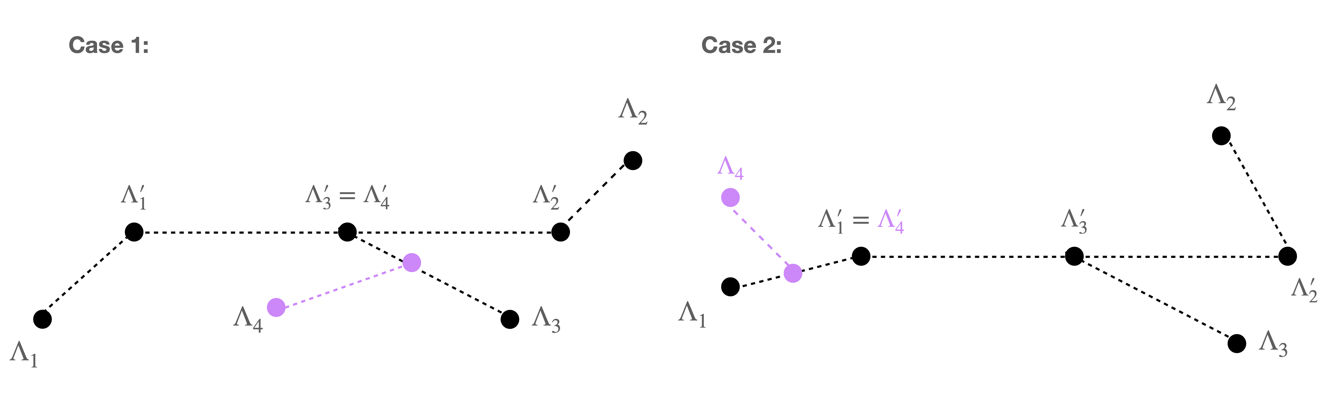
Figure 3. Case 1 and Case 2 in the proof of Corollary 3.18.

4. Computing the Distance From the Root

Let $\tilde{O}$ be a $q$-maximal $q$-enlargement of a suborder of $\text{End}(E)$. In this section, we show how to compute the distance between $\text{End}(E)\otimes\mathbb{Z}_{q}$ and $\tilde{O}\otimes\mathbb{Z}_{q}$, viewed as vertices on the Bruhat-Tits tree.

In the following proposition, we give a convenient expression for $\bigcap_{\Lambda\in N_{r}(M_{2}(\mathbb{Z}_{q}))}\Lambda$.

Proposition 4.1.

Fix an integer $r\geq 0$. Let $\tilde{\Lambda}=\cap_{\Lambda\in N_{r}(M_{2}(\mathbb{Z}_{q}))}\Lambda$. Then $\tilde{\Lambda}=\mathbb{Z}_{q}+q^{r}M_{2}(\mathbb{Z}_{q}).$

Proof.

We first give an explicit basis for $\tilde{\Lambda}$. For any $\gamma_{c}\in\Sigma$ as in the notation of Definition 3.3, we have $d(\gamma_{c}^{r},\operatorname{Id})=r$ by Proposition 3.8. Hence $\gamma_{c}^{-r}M_{2}(\mathbb{Z}_{q})\gamma_{c}^{r}\in N_{r}(M_{2}(\mathbb{Z}_{q}))$. It also follows that for $c\neq c^{\prime}$, $d(\gamma_{c}^{r},\gamma_{c^{\prime}}^{r})=2r$. In particular,

$$d_{3}(\{\gamma_{\infty}^{-r}M_{2}(\mathbb{Z}_{q})\gamma_{\infty}^{r},\gamma_{0}^{-r}M_{2}(\mathbb{Z}_{q})\gamma_{0}^{r},\gamma_{1}^{-r}M_{2}(\mathbb{Z}_{q})\gamma_{1}^{r},\gamma_{\infty}^{-r}M_{2}(\mathbb{Z}_{q})\gamma_{\infty}^{r}\})=6r.$$

By Corollary 3.18 and Lemma 3.15, we have $d_{3}(N_{r}(M_{2}(\mathbb{Z}_{q})))=6r$. It follows from Theorem 3.14 that

$$\tilde{\Lambda}=\gamma_{\infty}^{-r}M_{2}(\mathbb{Z}_{q})\gamma_{\infty}^{r}\cap\gamma_{0}^{-r}M_{2}(\mathbb{Z}_{q})\gamma_{0}^{r}\cap\gamma_{1}^{-r}M_{2}(\mathbb{Z}_{q})\gamma_{1}^{r}.$$

A basis of $\gamma_{\infty}^{-r}M_{2}(\mathbb{Z}_{q})\gamma_{\infty}^{r}\cap\gamma_{0}^{-r}M_{2}(\mathbb{Z}_{q})\gamma_{0}^{r}$ is

$$\biggl{\{}\begin{pmatrix}1&0\\ 0&1\end{pmatrix},q^{r}\begin{pmatrix}0&1\\ 0&0\end{pmatrix},q^{r}\begin{pmatrix}0&0\\ 1&0\end{pmatrix},\begin{pmatrix}0&0\\ 0&1\end{pmatrix}\biggl{\}}.$$

An element of $\gamma_{1}^{-r}M_{2}(\mathbb{Z}_{q})\gamma_{1}^{r}$ can be written as

$$a\begin{pmatrix}1&0\\ 0&1\end{pmatrix}+bq^{r}\begin{pmatrix}0&1\\ 0&0\end{pmatrix}+c\begin{pmatrix}-Aq^{-r}&q^{-r}\\ q^{-r}&0\end{pmatrix}+d\begin{pmatrix}0&-A\\ 0&1\end{pmatrix}$$

where $A\equiv 1\pmod{q^{r}}$. Hence an element is in the triple intersection if and only if $c\equiv 0\pmod{q^{2r}}$ and $d\equiv 0\pmod{q^{r}}$. In other words, a basis for the triple intersection is given by

$$\biggl{\{}\begin{pmatrix}1&0\\ 0&1\end{pmatrix},q^{r}\begin{pmatrix}0&1\\ 0&0\end{pmatrix},q^{r}\begin{pmatrix}-A&1\\ 1&0\end{pmatrix},q^{r}\begin{pmatrix}0&-A\\ 0&1\end{pmatrix}\biggl{\}},$$

which can be rewritten as

$$\biggl{\{}\begin{pmatrix}1&0\\ 0&1\end{pmatrix},q^{r}\begin{pmatrix}0&1\\ 0&0\end{pmatrix},q^{r}\begin{pmatrix}0&0\\ 1&0\end{pmatrix},q^{r}\begin{pmatrix}0&0\\ 0&1\end{pmatrix}\biggl{\}}.$$

∎

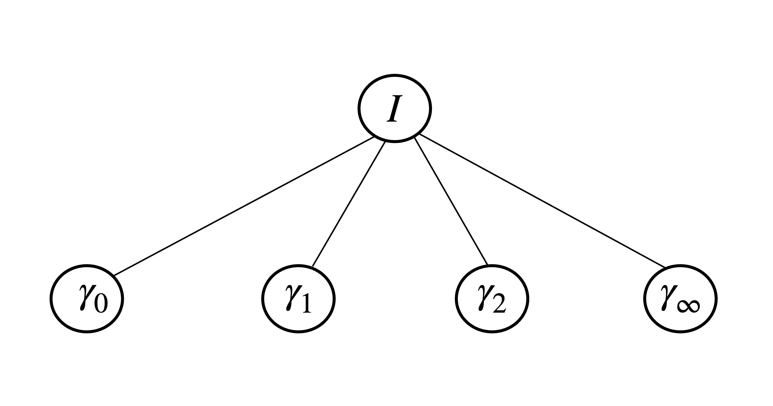
Figure 4. The maximal orders containing $\bigcap_{\Lambda^{\prime}\subset N_{1}(M_{2}(\mathbb{Z}_{q}))}\Lambda^{\prime}$ when $q=3$.

We will use Proposition 4.1 to compute the distance between $\tilde{O}$ and $\text{End}(E)\otimes\mathbb{Z}_{q}$ under an appropriate embedding into $M_{2}(\mathbb{Q}_{q})$. Namely, if $\tilde{O}\otimes\mathbb{Z}_{q}$ is mapped to the root of the Bruhat-Tits tree, the distance will be the least $r$ for which $\mathbb{Z}_{q}+q^{r}M_{2}(\mathbb{Z}_{q})\subset\text{End}(E)\otimes\mathbb{Z}_{q}$. We compute $r$ by finding the least $r$ for which $q^{r}\tilde{O}\subset\text{End}(E)$. We show that such an $r$ exists and is bounded in terms of the reduced discriminant of the input order.

Proposition 4.2.

Let $\mathcal{O}_{0}$ be an order, and let $\mathcal{O}$ be a $q$-enlargement of $\mathcal{O}_{0}$ for a prime $q$. If $k\geq v_{q}([\mathcal{O}:\mathcal{O}_{0}])$, then $q^{k}\mathcal{O}\subset\mathcal{O}_{0}$.

Proof.

For any prime $q^{\prime}$, the power of $q^{\prime}$ exactly dividing the global index $[\mathcal{O}:\mathcal{O}_{0}]$ is a generator for the local index at $q^{\prime}$, $[\mathcal{O}\otimes\mathbb{Z}_{(q^{\prime})}:\mathcal{O}_{0}\otimes\mathbb{Z}_{(q^{\prime})}]$, by [Voi21, Lemma 9.6.7]. As $\mathcal{O}$ is a $q$-enlargement of $\mathcal{O}_{0}$, we have $\mathcal{O}\otimes\mathbb{Z}_{q^{\prime}}=\mathcal{O}_{0}\otimes\mathbb{Z}_{q^{\prime}}$, and thus $\mathcal{O}_{0}\otimes\mathbb{Z}_{(q^{\prime})}=\mathcal{O}\otimes\mathbb{Z}_{(q^{\prime})}$ [Voi21, Lemma 9.5.3]. Hence $[\mathcal{O}\otimes\mathbb{Z}_{(q^{\prime})}:\mathcal{O}_{0}\otimes\mathbb{Z}_{(q^{\prime})}]$ is generated by a unit of $\mathbb{Z}_{(q^{\prime})}$ whenever $q^{\prime}\neq q$. Thus, the global index $[\mathcal{O}:\mathcal{O}_{0}]$ is a power of $q$. If $e=v_{q}(\operatorname{discrd}([\mathcal{O}:\mathcal{O}_{0}]))$, then $q^{e}\mathcal{O}\subset\mathcal{O}_{0}$. If $k\geq e$, then $q^{k}\mathcal{O}\subset q^{e}\mathcal{O}\subset\mathcal{O}_{0}$. ∎

Corollary 4.3.

Let $\mathcal{O}_{0}\subset\text{End}(E)$ be an order, and let $\tilde{\mathcal{O}}$ be a $q$-maximal $q$-enlargement of $\mathcal{O}_{0}$ for $q\neq p$. Let $e=v_{q}(\operatorname{discrd}(\mathcal{O}_{0}))$. Then $q^{e}\tilde{\mathcal{O}}\subset\text{End}(E)$.

Proof.

We have $\operatorname{discrd}(\mathcal{O}_{0})=[\tilde{\mathcal{O}}:\mathcal{O}_{0}]\operatorname{discrd}(\tilde{\mathcal{O}})$ by [Voi21, Lemma 15.2.15]. As $\tilde{\mathcal{O}}$ is maximal at $q$, and $q\neq p$, we have $v_{q}(\operatorname{discrd}(\tilde{\mathcal{O}}))=0$. Thus $e=v_{q}(\operatorname{discrd}(\mathcal{O}_{0}))=v_{q}([\tilde{\mathcal{O}}:\mathcal{O}_{0}])$. It now follows from Proposition 4.2 that $q^{e}\tilde{\mathcal{O}}\subset\mathcal{O}_{0}$, and since $\mathcal{O}_{0}\subset\text{End}(E)$ by hypothesis, we have $q^{e}\tilde{\mathcal{O}}\subset\text{End}(E)$. ∎

The next proposition shows that the distance can be computed without reference to an embedding into $M_{2}(\mathbb{Q}_{q})$.

Proposition 4.4.

Let $\mathcal{O}_{0}$ be a suborder of $\text{End}(E)$ and let $\tilde{\mathcal{O}}$ be a $q$-maximal $q$-enlargement of $\mathcal{O}_{0}$. Let $f$ be any isomorphism $f:\tilde{\mathcal{O}}\otimes\mathbb{Q}_{q}\to M_{2}(\mathbb{Q}_{q})$ such that $f(\tilde{\mathcal{O}}\otimes\mathbb{Z}_{q})=M_{2}(\mathbb{Z}_{q}).$ Let $\Lambda_{E}=f(\text{End}(E)\otimes\mathbb{Z}_{q})$. Let $r$ be the least integer such that $q^{r}\tilde{\mathcal{O}}\subset\text{End}(E)$. Then $r=d(M_{2}(\mathbb{Z}_{q}),\Lambda_{E})$.

Proof.

Let $f$ be any isomorphism satisfying the hypotheses of the proposition, and let $\Lambda_{E}=f(\text{End}(E)\otimes\mathbb{Z}_{q})$. Let $\tilde{\Lambda}=\cap_{\Lambda\in N_{k}(M_{2}(\mathbb{Z}_{q}))}\Lambda$. By Corollary 3.18, $d(M_{2}(\mathbb{Z}_{q}),\Lambda_{E})\leq k$ if and only if $\tilde{\Lambda}\subset\Lambda_{E}$. By Proposition 4.1, we have $\tilde{\Lambda}=\mathbb{Z}_{q}+q^{k}M_{2}(\mathbb{Z}_{q})$. This shows that $d(M_{2}(\mathbb{Z}_{q}),\Lambda_{E})$ is the least $r$ for which $\mathbb{Z}_{q}+q^{r}M_{2}(\mathbb{Z}_{q})\subset\Lambda_{E}$. We will now show that $\mathbb{Z}_{q}+q^{k}M_{2}(\mathbb{Z}_{q})\subset\Lambda_{E}$ if and only if $q^{k}\tilde{\mathcal{O}}\subset\text{End}(E)$.

As $\mathbb{Z}_{q}$ is contained in every $\mathbb{Z}_{q}$-order, we have $\mathbb{Z}_{q}+q^{k}M_{2}(\mathbb{Z}_{q})\subset\Lambda_{E}$ if and only if $q^{k}M_{2}(\mathbb{Z}_{q})\subset\Lambda_{E}$. By hypothesis, $q^{k}M_{2}(\mathbb{Z}_{q})=f(q^{k}\tilde{O}\otimes\mathbb{Z}_{q})$. It follows that $q^{k}M_{2}(\mathbb{Z}_{q})\subset\Lambda_{E}$ if and only if $q^{k}\tilde{O}\subset\text{End}(E)\otimes\mathbb{Z}_{q}$. Since $\tilde{O}$ is a $q$-maximal order, at primes $q^{\prime}\neq q$ we have $q^{k}\tilde{\mathcal{O}}\otimes\mathbb{Z}_{q^{\prime}}=\tilde{\mathcal{O}}\otimes\mathbb{Z}_{q^{\prime}}=\mathcal{O}_{0}\otimes\mathbb{Z}_{q^{\prime}}\subset\text{End}(E)\otimes\mathbb{Z}_{q^{\prime}}.$ It follows from the local-global principle that $q^{k}\tilde{\mathcal{O}}\subset\text{End}(E)$ if and only if $q^{k}\tilde{\mathcal{O}}\otimes\mathbb{Z}_{q}\subset\text{End}(E)\otimes\mathbb{Z}_{q}$. This shows that $d(M_{2}(\mathbb{Z}_{q}),\Lambda_{E})$ is the least $r$ for which $q^{r}\tilde{O}\subset\text{End}(E)$.∎

We now give an algorithm to compute the distance $d(M_{2}(\mathbb{Z}_{q}),\Lambda_{E})$, where $\Lambda_{E}$ is the image of $\text{End}(E)\otimes\mathbb{Z}_{q}$ under any isomorphism satisfying the hypotheses of Proposition 4.4. We will construct both $\tilde{\mathcal{O}}$ and $f$ in Section 5.

Algorithm 4.5.

Computing the distance $d(M_{2}(\mathbb{Z}_{q}),\Lambda_{E})$

Input: $E/\mathbb{F}_{p^{2}}$ supersingular; a basis $B$ for a $q$-maximal $q$-enlargement of $\mathcal{O}_{0}\subset\text{End}(E)$ with elements of $B$ expressed as elements of $\mathcal{O}_{0}\otimes\mathbb{Z}_{(q)}$; a prime $q\neq p$; $e:=v_{q}(\operatorname{discrd}(\mathcal{O}_{0}))$

Output: $r=d(M_{2}(\mathbb{Z}_{q}),\Lambda_{E})$

1. Set $i:=e-1$.

2. While $0\leq i\leq e-1$:

   1. Use Proposition 2.4 to determine if $q^{i}b\in\text{End}(E)$ for each $b\in B$.

   2. If for any $b\in B$, $q^{i}b\not\in\text{End}(E)$, output $i+1$. Otherwise, set $i:=i-1$.

3. Output $0$.

Proposition 4.6.

Algorithm 4.5 is correct and uses at most $4(e+1)$ applications of Proposition 2.4, with input $n=q$ and $\beta\in\text{End}(E)$. The run time is polynomial in $\log(p^{2})$ and $e\log(q)\max\{\log(\operatorname{Nrd}(b)):b\in B\}.$

Proof.

Let $\tilde{O}$ be the order generated by $B$. By Proposition 4.3, we have $q^{e}\tilde{\mathcal{O}}\subset\text{End}(E)$, so the least $r$ for which $q^{r}\tilde{\mathcal{O}}\subset\text{End}(E)$ is at most $e$. This shows that the output is the least $r$ for which $q^{r}\tilde{\mathcal{O}}\subset\text{End}(E)$. By Proposition 4.4, this is the distance $d(M_{2}(\mathbb{Z}_{q}),\Lambda_{E})$. In each iteration of the while loop, we apply Proposition 2.4 at most 4 times, and there are at most $e+1$ iterations of the while loop. At the $i$-th stage, we can express each candidate endomorphism as $\frac{q^{i+1}b}{q}$, where $q^{i+1}b\in\text{End}(E)$ was verified in the $(i-1)$-th stage. We have $\deg(q^{i+1}b)=q^{2(i+1)}\operatorname{Nrd}(b)$, so the run-time follows from Proposition 2.4.∎

5. Using Global Containment to Test Local Containment

In this section, we show how to translate between computations in $\text{End}(E)\otimes\mathbb{Q}$ and computations in the Bruhat-Tits tree. In the former, we have Proposition 2.4, and we would like to use this algorithm to deduce information about $\text{End}(E)\otimes\mathbb{Z}_{q}$. Using work of Voight, we construct a $q$-maximal $q$-enlargement $\tilde{O}$ of our input order and an isomorphism $f:\tilde{O}\otimes\mathbb{Z}_{q}\to M_{2}(\mathbb{Z}_{q})$. This maps the global order $\tilde{O}$ to the root of our Bruhat-Tits tree, so that $\tilde{O}\subset\text{End}(E)$ if and only if $M_{2}(\mathbb{Z}_{q})=f(\text{End}(E)\otimes\mathbb{Z}_{q})$. The main result of this section is Corollary 5.6, which shows that for any finite intersection of orders $\Lambda$ in $M_{2}(\mathbb{Q}_{q})$, we can construct a global order $O$ such that $O\subset\text{End}(E)$ if and only if $\Lambda\subset f(\text{End}(E)\otimes\mathbb{Z}_{q})$. This will allow us to test many candidates for $\text{End}(E)\otimes\mathbb{Z}_{q}$ at once.

First, we state the following propositions, which are due to [Voi13]. More details of the constructions are given in Appendix B.

Proposition 5.1.

Suppose an order $\mathcal{O}_{0}\subset\text{End}(E)$ is given by a basis and a multiplication table, and let $q$ be a prime. Then there is an algorithm which computes a $q$-maximal $q$-enlargement $\tilde{O}$ of $\mathcal{O}_{0}$. The run time is polynomial in the size of the basis and multiplication table. The basis elements which are output are of the form $\frac{\beta}{q^{k}}$, for an endomorphism $\beta\in\mathcal{O}_{0}$ and $k\leq e=v_{q}(\operatorname{discrd}(\mathcal{O}_{0}))$. Furthermore, $\log(\deg(\beta))$ is polynomial in the pairwise reduced traces of the basis elements of $\mathcal{O}_{0}$.

Proof.

This can be done using [Voi13, Algorithms 3.12, 7.9, 7.10].∎

Proposition 5.2.

Let $q\neq p$. Given a $q$-maximal order $\tilde{\mathcal{O}}\subset\text{End}(E)\otimes\mathbb{Q}$ and a nonnegative integer $r$, there is an algorithm which computes an isomorphism $f:\tilde{\mathcal{O}}\otimes\mathbb{Z}_{q}\to M_{2}(\mathbb{Z}_{q})$ modulo $q^{r+1}$. This isomorphism is specified by giving the inverse image of standard basis elements $i^{\prime}$ and $j^{\prime}$ determined mod $q^{r+1}$ in $\tilde{\mathcal{O}}$, such that

$$j^{\prime}\mapsto\begin{pmatrix}0&1\\ 1&0\end{pmatrix}$$

and

$$i^{\prime}\mapsto\begin{pmatrix}1&0\\ 0&-1\end{pmatrix}\text{ if }q\neq 2,\begin{pmatrix}0&1\\ 1&1\end{pmatrix}\text{ otherwise}.$$

The run time is polynomial in $\log(q^{r})$ and the size of the basis and multiplication table for $\tilde{\mathcal{O}}$. In terms of the basis for $\tilde{\mathcal{O}}$, the representatives $i^{\prime}$ and $j^{\prime}$ are expressed with coefficients which are determined mod $q^{r+1}$.

Proof.

The main steps are to compute a zero divisor mod $q^{r+1}$ and then to apply [Voi13, Algorithms 4.2, 4.3].∎

The other maximal orders that we will work with in the Bruhat-Tits tree are of the form $T^{-1}M_{2}(\mathbb{Z}_{q})T$, where $T$ is a matrix associated to a matrix path, as described in Definition 3.3. The next lemma shows that $T$ can be replaced with $T^{\prime}$ such that $T\equiv T^{\prime}\pmod{q^{r+1}}$, where $r>v_{q}(\det(T))$.

Lemma 5.3.

Let $T=\begin{pmatrix}q^{a}&c\\ 0&q^{b}\\ \end{pmatrix}$, with $a,b\geq 0$, $c\in\mathbb{Z}/q^{b}\mathbb{Z}$, and $v_{q}(c)=0$ if both $a$ and $b$ are positive. Let $T^{\prime}=T+q^{e}M$ where $M\in M_{2}(\mathbb{Z}_{q})$ and $e>a+b$. Then there is $x\in\mathbb{Q}_{q}^{*}$ and $C\in\operatorname{GL}_{2}(\mathbb{Z}_{q})$ such that $T=xCT^{\prime}$. In particular, $T^{-1}M_{2}(\mathbb{Z}_{q})T=T^{\prime-1}M_{2}(\mathbb{Z}_{q})T^{\prime}$.

Proof.

We write $T^{\prime}=\begin{pmatrix}q^{a}+dq^{e}&c+fq^{e}\\ gq^{e}&q^{b}+hq^{e}\end{pmatrix}$ with $d,f,g,h\in\mathbb{Z}_{q}$.

Multiplying on the left by $\begin{pmatrix}(1+dq^{e-a})^{-1}&0\\ -gq^{e-a}(1+dq^{e-a})^{-1}&1\end{pmatrix}\in\operatorname{GL}_{2}(\mathbb{Z}_{q})$ gives $\begin{pmatrix}q^{a}&\alpha\\ 0&q^{b}\beta\end{pmatrix},$ where $\alpha=(c+fq^{e})(1+dq^{e-a})^{-1}$ and $\beta=1+hq^{e-a}-gq^{e-a-b}\alpha$.

By choice of $e$, we have $v_{q}(\beta)=0$ and $v_{q}(\alpha)\geq 0$. We also have $c=\alpha+q^{b}(dq^{e-a-b}\alpha-fq^{e-b})$. Multiply on the left by $\begin{pmatrix}1&\beta^{-1}(dq^{e-a-b}\alpha-fq^{e-b})\\ 0&\beta^{-1}\end{pmatrix}\in\operatorname{GL}_{2}(\mathbb{Z}_{q})$ to arrive at $T$. All operations are invertible over $\mathbb{Z}_{q}$ provided $e>a+b$. ∎

To check that a finite intersection of local maximal orders is contained in $\text{End}(E)\otimes\mathbb{Z}_{q}$, we will check that the intersection of related maximal orders is contained in $\text{End}(E)$. The following lemma allows us to compute the basis of an intersection of $\mathbb{Z}$-orders in polynomial time.

Lemma 5.4.

Let $L_{1},L_{2}\subseteq\mathbb{Z}^{4}$ be two $\mathbb{Z}$-lattices of full rank, specified by a possibly dependent set of generators. A basis for each lattice, a lattice basis for the sum $L_{1}+L_{2}$ and for the intersection $L_{1}\cap L_{2}$ can be computed in polynomial time.

Proof.

A basis for each lattice from a set of $m$ generators can be computed by writing the generators as the columns of a matrix and the compute the Hermite Normal Form (HNF) of the matrix (see [MG02, p. 149] for the definition. The HNF of this $4\times m$ matrix can be computed in time polynomial in $m$, and the bit length of the matrix entries, see [HM91, MW01]. Computing a basis for the sum of two lattices immediately reduces to the problem of computing a basis of a lattice from a set of generators. To compute the intersection of two lattices $L_{1},L_{2}$ each specified by a $4\times 4$ basis in matrix form $B_{1},B_{2}$, we first compute $(B_{1}^{T})^{-1}$ and $(B_{2}^{T})^{-1}$. Here $B_{i}^{T}$ denotes the transpose of $B_{i}$. The matrix $(B_{i}^{T})^{-1}$ is a basis for the dual $\hat{L_{i}}$ of $L_{i}$ [MG02, p. 19]. By Cramer’s rule, the inverse of this $4\times 4$ matrix can be computed efficiently. Since the dual of a lattice $L$ consists of all vectors $y$ in $L\otimes\mathbb{R}$ whose real inner product $\langle x,y\rangle$ is an integer for every $x\in L$, it follows easily that the dual of $L_{1}\cap L_{2}$ is $\hat{L}_{1}+\hat{L}_{2}$, i.e. the smallest lattice containing both $\hat{L_{1}}$ and $\hat{L_{2}}$. So a basis for the intersection is obtained by computing a basis for the lattice $\tilde{L}:=\hat{L}_{1}$ and $\hat{L}_{2}$ and then computing the dual of $\tilde{L}$. By the above argument, this can be computed in polynomial time. ∎

Corollary 5.5.

Let $\mathcal{O}(i),i=1,\dots,3$ be orders in $B_{p,\infty}$ such that $(\operatorname{disc}(\mathcal{O}_{0}))\mathcal{O}_{0}\subseteq\mathcal{O}(i)$. A basis for $\cap\mathcal{O}(i)$ in which each basis vector is given as a $\mathbb{Q}$-linear combination of the basis vectors for $\mathcal{O}_{0}$ can be computed in polynomial time.

Proof.

We can reduce this to matrix computations with $4\times 4$ integer matrices and use the previous lemma. We identify our starting global order $\mathcal{O}_{0}$ with $\mathbb{Z}^{4}$, whose Hermite Normal Form is just the $4\times 4$ identity matrix. Since $(\operatorname{disc}(\mathcal{O}_{0}))\mathcal{O}_{0}\subseteq\mathcal{O}(i)$, we can scale the matrices representing the orders $\mathcal{O}(i)$ by $\operatorname{disc}\mathcal{O}_{0}$ and work with integer matrices. See [Coh93, page 73f.] for generalizing the computation of the HNF to matrices with bounded rational coefficients. By the previous lemma, $\cap\mathcal{O}(i)$ can be computed in polynomial time. ∎

The following is the main result of this section, which shows that we can check local containment by checking global containment.

Corollary 5.6.

Let $\mathcal{O}_{0}\subset\text{End}(E)$. Let $\Lambda$ be a finite intersection of maximal orders of $M_{2}(\mathbb{Q}_{q})$, and let $r\leq v_{q}(\operatorname{discrd}(\mathcal{O}_{0}))$ be an integer such that $\Lambda\subset\cap_{\Lambda^{\prime}\in N_{r}(M_{2}(\mathbb{Z}_{q}))}\Lambda^{\prime}$. Let $\tilde{\mathcal{O}}$ be a q-maximal q-enlargement of $\mathcal{O}_{0}$ and let $f$ be the isomorphism computed in Proposition 5.2. Then there exists a global order $\mathcal{O}$ such that $\mathcal{O}\subset\text{End}(E)$ if and only if $\Lambda\subset f(\text{End}(E)\otimes\mathbb{Z}_{q})$. The basis of $\mathcal{O}$ can be computed in polynomial time in the size of $\mathcal{O}_{0}$ and $\log(q)$, and the basis elements of $\mathcal{O}$ have degree polynomial in the size of $\mathcal{O}_{0}$ and $q^{r}$.

Proof.

We will show that $\mathcal{O}$ can be computed such that $f(\mathcal{O}\otimes\mathbb{Z}_{q})=\Lambda$ and $\mathcal{O}\otimes\mathbb{Z}_{q^{\prime}}\subset\mathcal{O}_{0}\otimes\mathbb{Z}_{q^{\prime}}$ for all primes $q^{\prime}\neq q$.

Suppose that $\Lambda$ is maximal. Write $\Lambda=T^{-1}M_{2}(\mathbb{Z}_{q})T$ where $T$ is the matrix associated to a matrix path of length at most $r$, written $T=\begin{pmatrix}q^{a}&c\\ 0&q^{b}\end{pmatrix}$ where $a+b\leq r$.

We construct an element $t\in\tilde{\mathcal{O}}$ such that $f(t)\equiv T\pmod{q^{r+1}}$. Let $i^{\prime},j^{\prime}\in\tilde{\mathcal{O}}$ denote the inverse image of the standard basis elements of $M_{2}(\mathbb{Z}_{q})$ modulo $q^{r+1}$, as in Proposition 5.2. If $q$ is odd, then with $f(i^{\prime})\equiv\begin{pmatrix}1&0\\ 0&-1\end{pmatrix}\pmod{q^{r+1}}$ and $f(j^{\prime})\equiv\begin{pmatrix}0&1\\ 1&0\end{pmatrix}\pmod{q^{r+1}}$, we can take

$$t=\frac{q^{a}+q^{b}}{2}+\frac{q^{a}-q^{b}}{2}i^{\prime}+\frac{c}{2}j^{\prime}+\frac{c}{2}i^{\prime}j^{\prime}.$$

As written, $t$ is an element of $\tilde{\mathcal{O}}\otimes\mathbb{Q}$, but we can replace division by 2 with multiplication by an integer $m\equiv 2^{-1}\pmod{q^{r+1}}$ to ensure $t\in\tilde{\mathcal{O}}$ and $f(t)\equiv T\pmod{q^{r+1}}$. If $q=2$, then with $f(i^{\prime})\equiv\begin{pmatrix}0&1\\ 1&1\end{pmatrix}\pmod{q^{r+1}}$ and $f(j^{\prime})\equiv\begin{pmatrix}0&1\\ 1&0\end{pmatrix}\pmod{q^{r+1}}$, we can take

$$t=(q^{a}+c)+(q^{b}-q^{a})i^{\prime}+(c-q^{b}+q^{a})j^{\prime}+(-c)i^{\prime}j^{\prime}.$$

Let $\mathcal{O}=\frac{1}{q^{a+b}}\hat{t}\tilde{\mathcal{O}}t$, where $\hat{}$ denotes the dual isogeny. At $q^{\prime}\neq q$, we have $\mathcal{O}\otimes\mathbb{Z}_{q^{\prime}}\subset\mathcal{O}_{0}\otimes\mathbb{Z}_{q^{\prime}}\subset\text{End}(E)\otimes\mathbb{Z}_{q^{\prime}}$. This is because $\tilde{\mathcal{O}}\otimes\mathbb{Z}_{q^{\prime}}=\mathcal{O}_{0}\otimes\mathbb{Z}_{q^{\prime}}$, and $\hat{t}\tilde{\mathcal{O}}t\subset\tilde{\mathcal{O}}$. At $q$, we have $f(\mathcal{O}\otimes\mathbb{Z}_{q})=T^{-1}M_{2}(\mathbb{Z}_{q})T\supset f(\mathcal{O}_{0}\otimes\mathbb{Z}_{q})$. By the local-global principle, we get $f(\mathcal{O}\otimes\mathbb{Z}_{q})\subset f(\text{End}(E)\otimes\mathbb{Z}_{q})$ if and only if $\mathcal{O}\subset\text{End}(E)$.

In the general case, let $\Lambda_{1},\Lambda_{2},\Lambda_{3}$ be maximal orders in $M_{2}(\mathbb{Q}_{q})$ such that $\Lambda=\cap_{i=1}^{3}\Lambda_{i}$. We can choose three orders $\Lambda_{i}$ for which this is true by Theorem 3.14. Let $\mathcal{O}(i)$ denote a global order such that $\mathcal{O}(i)\otimes\mathbb{Z}_{q^{\prime}}\subset\mathcal{O}_{0}\otimes\mathbb{Z}_{q^{\prime}}$ for all $q^{\prime}\neq q$ and $f(\mathcal{O}(i)\otimes\mathbb{Z}_{q})=\Lambda_{i}$, as constructed in the previous paragraph.

Let $\mathcal{O}=\cap_{i=1}^{3}\mathcal{O}(i)$. By construction, $q^{a+b}\mathcal{O}(i)\subset\tilde{\mathcal{O}}$, and by Corollary 4.3, we have $q^{v_{q}(\operatorname{discrd}(\mathcal{O}_{0}))}\tilde{\mathcal{O}}\subset\mathcal{O}_{0}$. As $a+b\leq r\leq v_{q}(\operatorname{discrd}(\mathcal{O}_{0}))$, we have $q^{2v_{q}(\operatorname{discrd}(\mathcal{O}_{0}))}\mathcal{O}(i)\subset\mathcal{O}_{0}$, and thus $\operatorname{disc}(\mathcal{O}_{0})\mathcal{O}(i)\subset\mathcal{O}_{0}$. By Corollary 5.5, the basis of $\mathcal{O}$ can be computed in polynomial time.

Tensoring by $\mathbb{Z}_{q^{\prime}}$ for any prime $q^{\prime}$ commutes with taking intersections, as $\mathbb{Z}_{q^{\prime}}$ is a flat $\mathbb{Z}$-module. Hence $\mathcal{O}\otimes\mathbb{Z}_{q^{\prime}}=\cap_{i=1}^{3}\mathcal{O}(i)\otimes\mathbb{Z}_{q^{\prime}}\subset\mathcal{O}_{0}\otimes\mathbb{Z}_{q^{\prime}}$ for all $q^{\prime}\neq q$, and $f(\mathcal{O}\otimes\mathbb{Z}_{q})=\cap_{i=1}^{3}f(\mathcal{O}(i)\otimes\mathbb{Z}_{q})=\cap_{i=1}^{3}\Lambda_{i}=\Lambda$.

We have that $\mathcal{O}\otimes\mathbb{Z}_{q^{\prime}}\subset\mathcal{O}_{0}\otimes\mathbb{Z}_{q^{\prime}}\subset\text{End}(E)\otimes\mathbb{Z}_{q^{\prime}}$ for all $q^{\prime}\neq q$, so $\mathcal{O}\subset\text{End}(E)$ if and only if $\mathcal{O}\otimes\mathbb{Z}_{q}\subset\text{End}(E)\otimes\mathbb{Z}_{q}$. As $f$ is an isomorphism, this is equivalent to $\Lambda\subset f(\text{End}(E)\otimes\mathbb{Z}_{q})$, as desired.∎

6. Finding $\Lambda_{E}$ in the Bruhat-Tits Tree

Let $\Lambda_{E}=f(\text{End}(E)\otimes\mathbb{Z}_{q})$ and $r=d(\Lambda_{E},M_{2}(\mathbb{Z}_{q}))$. Once we have computed $r$, we know that $\Lambda_{E}$ is of the form $T^{-1}M_{2}(\mathbb{Z}_{q})T$, where $T$ is a matrix associated to a matrix path of length $r$. In this section, we show how to recover the matrix path one step at a time, which will allow us to compute $\Lambda_{E}$.

For each matrix path $\{c_{i}\}_{i=1}^{k}$ of length at most $r$, the next two propositions define an order which is contained in $\Lambda_{E}$ if and only if the corresponding path begins with $\{c_{i}\}_{i=1}^{k}$.

Proposition 6.1.

Let $q>2$. Let $\gamma$ be the matrix associated to a matrix path $\{c_{i}\}_{i=1}^{k}$, where $1\leq k\leq r.$ Let

$$S:=N_{r}(M_{2}(\mathbb{Z}_{q}))\cap\{\Lambda^{\prime}:\Lambda^{\prime}\text{ maximal corresponding to a matrix path starting with }\{c_{i}\}_{i=1}^{k}\}.$$

Let $\Lambda_{\gamma,r}:=\bigcap_{\Lambda\in S}\Lambda$ and $P=\{\gamma^{-1}M_{2}(\mathbb{Z}_{q})\gamma\}$. Then:

1. $\Lambda_{\gamma,r}=\bigcap_{\Lambda\in N_{r-k}(P)}\Lambda$.

2. $v_{q}(\operatorname{discrd}(\Lambda_{\gamma,r}))=3r-3k$.

3. Suppose $\Lambda_{\gamma,r}\subset\Lambda$ for a maximal order $\Lambda\in N_{r}(M_{2}(\mathbb{Z}_{q}))$. Then $\Lambda$ corresponds to a matrix path starting with $\{c_{i}\}_{i=1}^{k}$.

Proof.

Any order in $S$ corresponds to a matrix path $\{c_{1},\ldots,c_{k},b_{1},b_{2},\ldots,b_{r-k}\}$. Letting $\delta=b_{r-k}b_{r-k-1}\cdots b_{1}$, the associated matrix is $\delta\gamma$. By Proposition 3.8, we have $d(\gamma,\delta\gamma)=r-k$. This shows that $S\subset N_{r-k}(P)$. To show $\Lambda_{\gamma,r}=\bigcap_{\Lambda\in N_{r-k}(P)}\Lambda$, we will choose $\Lambda_{1}\Lambda_{2},\Lambda_{3}$ in $S$ which maximize $d_{3}$ among the orders of $N_{r-k}(P)$ and therefore in $S$. Choose three distinct matrices $\delta_{i}\in\Sigma$ such that $\delta_{i}c_{k}\not\in M_{2}(q\mathbb{Z}_{q})$. There are $q\geq 3$ possibilities for $\delta_{i}$. Let $\Lambda_{i}=(\delta_{i}^{r-k}\gamma)^{-1}M_{2}(\mathbb{Z}_{q})\delta_{i}^{r-k}\gamma$. If $i\neq j$, we have $d(\delta_{i}^{r-k}\gamma,\delta_{j}^{r-k}\gamma)=2r-2k$ by Proposition 3.8.

As $\delta_{i}c_{k}\not\in M_{2}(q\mathbb{Z}_{q})$, the matrices $\delta_{i}^{r-k}\gamma$ correspond to matrix paths of length $r$ starting with $\{c_{i}\}_{i=1}^{k}$, so $\Lambda_{i}\in S$. Therefore, $d_{3}(\{\Lambda_{1},\Lambda_{2},\Lambda_{3}\})=6r-6k\leq d_{3}(S)$.

By Corollary 3.18, we have $d_{3}(N_{r-k}(P))=6r-6k$, so $d_{3}(\Lambda_{1},\Lambda_{2},\Lambda_{3})=d_{3}(N_{r-k}(P))=d_{3}(S)$. By Theorem 3.14, this shows $\Lambda_{\gamma,r}=\Lambda_{1}\cap\Lambda_{2}\cap\Lambda_{3}=\cap_{\Lambda\subset N_{r-k}(P)}\Lambda$, which gives (1) and (2).

It follows from (1) and Corollary 3.18 that the set of maximal orders containing $\Lambda_{\gamma,r}$ is $N_{r-k}(P)$. To show (3), we must show that $N_{r}(M_{2}(\mathbb{Z}_{q}))\cap N_{r-k}(\gamma^{-1}M_{2}(\mathbb{Z}_{q})\gamma)$ consists of those orders corresponding to a matrix path of length $r$ starting with $\{c_{i}\}_{i=1}^{k}$.

Consider a matrix path $\{g_{i}\}_{i=1}^{r}$ and the associated matrix $g=g_{r}g_{r-1}\cdots g_{1}$. The order $g^{-1}M_{2}(\mathbb{Z}_{q})g$ is in the intersection $N_{r}(M_{2}(\mathbb{Z}_{q}))\cap N_{r-k}(\gamma^{-1}M_{2}(\mathbb{Z}_{q})\gamma)$ if and only if $d(g,\gamma)\leq r-k$. But by Lemma 3.8, $d(g,\gamma)\leq r-k$ if and only if the sequences agree in the first $k$ matrices, which are exactly $\{c_{i}\}_{i=1}^{k}.$ This shows (3).∎

Proposition 6.2.

Let $q=2$. Let $\gamma$ be the matrix associated to a matrix path $\{c_{i}\}_{i=1}^{k}$, where $1\leq k\leq r.$ Let

$$S:=N_{r}(M_{2}(\mathbb{Z}_{q}))\cap\{\Lambda^{\prime}:\Lambda^{\prime}\text{ maximal corresponding to a matrix path starting with }\{c_{i}\}_{i=1}^{k}\}.$$

Let $\Lambda_{\gamma,r}:=\cap_{\Lambda\in S}\Lambda$ and $\delta_{1},\delta_{2}\in\Sigma$ be such that $\delta_{1}c_{k}\not\in M_{2}(q\mathbb{Z}_{q})$ and $\delta_{2}c_{k}\not\in M_{2}(q\mathbb{Z}_{q})$. Let $P:=\{(\delta_{1}\gamma)^{-1}M_{2}(\mathbb{Z}_{q})\delta_{1}\gamma,\gamma^{-1}M_{2}(\mathbb{Z}_{q})\gamma,(\delta_{2}\gamma)^{-1}M_{2}(\mathbb{Z}_{q})\delta_{2}\gamma\}.$ Then:

1. $\Lambda_{\gamma,r}=\bigcap_{\Lambda\in N_{r-k-1}(P)}\Lambda$.

2. $v_{q}(\operatorname{discrd}(\Lambda_{\gamma,r}))=3r-3k-1$.

3. Suppose $\Lambda_{\gamma}\subset\Lambda$ for a maximal order $\Lambda$ such that $d(\Lambda,M_{2}(\mathbb{Z}_{q}))=r$. Then $\Lambda$ corresponds to a matrix path starting with $\{c_{i}\}_{i=1}^{k}$.

Proof.

Any order in $S$ corresponds to a matrix path $\{c_{1},\ldots,c_{k},\delta_{i},b_{1},b_{2},\ldots,b_{r-k-1}\}$ for one of $i=1,2$. Letting $\delta=b_{r-k-1}b_{r-k}\cdots b_{1}$, the associated matrix is $\delta\delta_{i}\gamma$. By Proposition 3.8, $d(\delta_{i}\gamma,\delta\delta_{i}\gamma)=r-k-1$. This shows $S\subset N_{r-k}(P)$. To show $\Lambda_{\gamma,r}=\bigcap_{\Lambda\in N_{r-k}(P)}\Lambda$, we will choose $\Lambda_{1}\Lambda_{2},\Lambda_{3}$ in $S$ which maximize $d_{3}$ among the orders of $N_{r-k-1}(P)$ and hence in $S$.

Let $\Lambda_{1}=(\delta_{1}^{r-k}\gamma)^{-1}M_{2}(\mathbb{Z}_{q})\delta_{1}^{r-k}\gamma$, and $\Lambda_{2}=(\delta_{2}^{r-k}\gamma)^{-1}M_{2}(\mathbb{Z}_{q})(\delta_{2}^{r-k}\gamma)$. Choose $\delta_{3}\in\Sigma$ such that $\delta_{3}\delta_{1}\not\in M_{2}(q\mathbb{Z}_{q})$ and $\delta_{3}\neq\delta_{1}$. Let $\Lambda_{3}=(\delta_{3}^{r-k-1}\delta_{1}\gamma)^{-1}M_{2}(\mathbb{Z}_{q})(\delta_{3}^{r-k-1}\delta_{1}\gamma)$. It is easy to see that $\Lambda_{i}\in S$ for each $i$, as the corresponding matrix paths have length $r$ and begin with $\{c_{i}\}_{=1}^{k}$. By Proposition 3.8, we compute $d_{3}(\{\Lambda_{1},\Lambda_{2},\Lambda_{3}\})=2(r-k)+2(r-k)+2(r-k-1)=6r-6k-2$.

By Corollary 3.18, $d_{3}(N_{r-k-1}(P))=6r-6k-2$, so $d_{3}(\Lambda_{1},\Lambda_{2},\Lambda_{3})=d_{3}(N_{r-k-1}(P))=d_{3}(S)$. By Theorem 3.14, this shows $\Lambda_{\gamma,r}=\Lambda_{1}\cap\Lambda_{2}\cap\Lambda_{3}=\cap_{\Lambda\subset N_{r-k}(P)}\Lambda$, which gives (1) and (2).

It follows from (1) and Corollary 3.18 that the set of maximal orders containing $\Lambda_{\gamma,r}$ is $N_{r-k-1}(P)$. To show (3), we must show that $N_{r}(M_{2}(\mathbb{Z}_{q}))\cap N_{r-k-1}(P)$ consists of those orders corresponding to a matrix path of length $r$ starting with $\{c_{i}\}_{i=1}^{k}$.

Consider a matrix path $\{g_{i}\}_{i=1}^{r}$ and the associated matrix $g=g_{r}g_{r-1}\cdots g_{1}$. The order $g^{-1}M_{2}(\mathbb{Z}_{q})g$ is in the intersection $N_{r}(M_{2}(\mathbb{Z}_{q}))\cap N_{r-k-1}(P)$ if and only if one of $d(g,\delta_{i}\gamma)\leq r-k-1$ or $d(g,\gamma)\leq r-k-1$. Since $\gamma$ corresponds to a matrix path of length $k$ and $g$ corresponds to a matrix path of length $r$, we have $d(g,\gamma)\geq r-k$, so the condition $d(g,\gamma)\leq r-k-1$ is impossible in this setup. We also have $d(g,\delta_{i}\gamma)\leq r-k-1$ if and only if $g_{i}=c_{i}$ for all $1\leq i\leq k$ and $c_{k+1}=\delta_{i}$. Since $\delta_{1}$ and $\delta_{2}$ are the only two choices for the $(k+1)$-th entry in a matrix path starting with $\{c_{i}\}_{i=1}^{k}$, we have $d(g,P)\leq r-k-1$ if and only if $g_{i}=c_{i}$ for all $1\leq i\leq k$. This shows (3).∎

We obtain the following algorithm to recover the matrix path $\{d_{i}\}_{i=1}^{r}$ corresponding to $\Lambda_{E}$. For each $\gamma_{c}$ as in Definition 3.3, we check if $\Lambda_{\gamma_{c},r}\subset\Lambda_{E}$. By Propositions 6.1 and  6.2, we have $\Lambda_{\gamma_{c},r}\subset\Lambda_{E}$ if and only if $d_{1}=\gamma_{c}$, so we recover the first matrix in the path in $q+1$ checks. Once we have recovered the first $k-1$ matrices, we test each of the $q$ possibilities for $d_{k}$, continuing until we have recovered the full matrix path.

Algorithm 6.3.

Computing the path from $M_{2}(\mathbb{Z}_{q})$ to $\Lambda_{E}$

Input: An order $\mathcal{O}_{0}\subset\text{End}(E)$; a prime $q\neq p$; $q$-maximal $q$-enlargement $\tilde{\mathcal{O}}$ of $\mathcal{O}_{0}$; an isomorphism $f:\mathcal{O}_{0}\otimes\mathbb{Q}_{q}\to M_{2}(\mathbb{Q}_{q})$ such that $f(\tilde{\mathcal{O}}\otimes\mathbb{Z}_{q})=M_{2}(\mathbb{Z}_{q})$ computed mod $q^{r+1}$; $r:=d(M_{2}(\mathbb{Z}_{q}),\Lambda_{E})$

Output: $\gamma$ such that $\Lambda_{E}=\gamma^{-1}M_{2}(\mathbb{Z}_{q})\gamma$

1. Set $k:=1$, $\gamma^{\prime}:=\operatorname{Id}$, $d_{0}:=\operatorname{Id}$.

2. While $k\leq r$:

   1. For each $\gamma_{c}\in\Sigma$ as in Definition 3.3 such that $\gamma_{c}d_{k-1}\not\in qM_{2}(\mathbb{Z}_{q})$:

      1. Set $\gamma:=\gamma_{c}\gamma^{\prime}$.

      2. Compute a basis $B_{\gamma}$ for an order $\mathcal{O}_{\gamma}$ such that $\mathcal{O}_{\gamma}\subset\text{End}(E)$ if and only if $\Lambda_{\gamma,r}\subset\Lambda_{E}$. (See Corollary 5.6.)

      3. Apply Proposition 2.4 to each $b\in B_{\gamma}$ to decide if $b\in\text{End}(E)$.

      4. If for all $b\in B_{\gamma}$, we have $b\in\text{End}(E)$: Set $\gamma^{\prime}:=\gamma$, $d_{k}:=\gamma_{c}$, $k:=k+1$, and return to Step 2.

3. Output $\gamma$.

Figure 5. Algorithm 6.3 Step 2 with $q=2$ and $d(\Lambda_{E},M_{2}(\mathbb{Z}_{q})))=3$.

Proposition 6.4.

Algorithm 6.3 is correct and requires at most $4(rq+1)$ applications of Proposition 2.4. In each application, the input for the algorithm in Proposition 2.4 has $n=q^{3}$ and $\beta$ with $\log(\deg(\beta))$ polynomially-sized in $\log(q^{r})$ and the size of $\mathcal{O}_{0}$.

Proof.

We know that for some $T_{E}=d_{r}d_{r-1}\cdots d_{1}$, we have $\Lambda_{E}=T_{E}^{-1}M_{2}(\mathbb{Z}_{q})T_{E}$. We show that $T_{E}$ is the output of the algorithm.

Let $\gamma=c_{k}\cdots c_{1}$. By the construction in Corollary 5.6, we have $\mathcal{O}_{\gamma}\subset\text{End}(E)$ if and only if $\Lambda_{\gamma}\subset\Lambda_{E}$. By Proposition 6.1(3) and 6.2(3), we have $\Lambda_{c_{k}\cdots c_{2}c_{1}}\subset\Lambda_{E}$ if and only if $c_{i}=d_{i}$ for each $i\leq k$. Therefore, Step 2(a)(iv) has $b\in\text{End}(E)$ for all $b\in B_{\gamma}$ if and only if $c_{i}=d_{i}$ for each $i\leq k$. The output after the $k=r$ step must be $\gamma=d_{r}d_{r-1}\cdots d_{1}=T_{E}$, as desired.

When $k=1$, there are $q+1$ choices for $\gamma_{c}$. For $1<k\leq r$, there are $q$ choices for $\gamma_{c}$. Thus, we test $\mathcal{O}_{\gamma}\subset\text{End}(E)$ for at most $rq+1$ values of $\gamma$.

If $\gamma=\gamma_{c}\gamma^{\prime}$, then a basis for $\mathcal{O}_{\gamma}$ can be written as a $\mathbb{Z}_{(q)}$-linear combination of elements of $\mathcal{O}_{\gamma^{\prime}}+\mathcal{O}_{0}.$ The exponent of $q$ in the denominator is at most 3, since $v_{q}([\Lambda_{\gamma}:\Lambda_{\gamma^{\prime}}])=v_{q}\operatorname{discrd}(\Lambda_{\gamma^{\prime}})-v_{q}\operatorname{discrd}(\Lambda_{\gamma}))=3$ by Propositions 6.1(2) and  6.2(2), and $\mathcal{O}_{\gamma}\otimes\mathbb{Z}_{q^{\prime}}\subset\mathcal{O}_{0}\otimes\mathbb{Z}_{q^{\prime}}$ when $q^{\prime}\neq q$ by construction. As the previous step verifies that $\mathcal{O}_{\gamma^{\prime}}\subset\text{End}(E)$, this shows that elements of $B_{\gamma}$ can be expressed as $\frac{\beta}{n}$ for $\beta\in\text{End}(E)$ and $n=q^{3}$. By Corollary 5.6, we have that $\log(\deg(\beta))$ is polynomially-sized in $\log(q^{r})$ and the size of $\mathcal{O}_{0}$. ∎

7. Bass Orders

Let $\Lambda_{0}=f(\mathcal{O}_{0}\otimes\mathbb{Z}_{q})$ and $\Lambda_{E}=f(\text{End}(E)\otimes\mathbb{Z}_{q})$. If $\Lambda_{0}$ is Bass, the subgraph of maximal orders containing $\Lambda_{0}$ forms a path which can be recovered efficiently. In this case, we can give a simpler algorithm which performs a binary search along the path to find $\Lambda_{E}$.

Algorithm 7.1.

Finding $\Lambda_{E}$ When $\Lambda_{0}$ is Bass

Input: An order $\mathcal{O}_{0}\subset\text{End}(E)$ which is Bass at $q$; $e=v_{q}(\operatorname{discrd}(\mathcal{O}_{0}))$

Output: $\gamma$ such that $\Lambda_{E}=\gamma^{-1}M_{2}(\mathbb{Z}_{q})\gamma$

1. Compute a $q$-maximal $q$-enlargement $\tilde{\mathcal{O}}\supset\mathcal{O}_{0}$ and an isomorphism $f:\tilde{\mathcal{O}}\otimes\mathbb{Q}_{q}\to M_{2}(\mathbb{Q}_{q})$ such that $f(\tilde{\mathcal{O}}\otimes\mathbb{Z}_{q})=M_{2}(\mathbb{Z}_{q})$ up to precision $q^{e+1}$. Set $\Lambda_{0}:=f(\mathcal{O}_{0}\otimes\mathbb{Z}_{q})$.

2. Compute a list $L$ of matrices $T_{i}$ associated to matrix paths such that $\Lambda_{0}\subset T_{i}^{-1}M_{2}(\mathbb{Z}_{q})T_{i}$. Index the matrices $T_{i}$, starting with $i=1$, such that $T_{i}$ and $T_{i+1}$ are adjacent in the Bruhat-Tits tree.

3. While $|L|>1$:

   1. Set $m:=\lfloor\frac{|L|}{2}\rfloor$, $\Lambda_{\text{start}}:=T_{1}^{-1}M_{2}(\mathbb{Z}_{q})T_{1}$, and $\Lambda_{\text{mid}}:=T_{m}^{-1}M_{2}(\mathbb{Z}_{q})T_{m}$.

   2. Compute a basis $B$ for an order $\mathcal{O}$ such that $f(\mathcal{O}\otimes\mathbb{Z}_{q})=\Lambda_{\text{start}}\cap\Lambda_{\text{mid}}$ and $\mathcal{O}\otimes\mathbb{Z}_{q^{\prime}}\subset\mathcal{O}_{0}\otimes\mathbb{Z}_{q^{\prime}}$ for all $q^{\prime}\neq q$. (Corollary 5.6)

   3. For each $b\in B$, use Proposition 2.4 to determine if $b\in\text{End}(E)$.

   4. If $b\in\text{End}(E)$ for all $b$, set $L:=\{T_{i}:1\leq i\leq m\}$. Otherwise, set $L:=\{T_{i}:m<i\leq|L|\}$, and reindex the matrices, by replacing the index $i+m$ with the index $i$ for $1\leq i\leq|L|-m$.

4. Output the single element of $L$.

Proposition 7.2.

Algorithm 7.1 is correct, requires at most $4\log_{2}(e+1)$ applications of Proposition 2.4, and runs in polynomial time in $\log(q)$ and the size of $\mathcal{O}_{0}$.

Proof.

Step 1 can be done in polynomial-time by Propositions 5.1 and 5.2. The list $L$ has size at most $e+1$, the orders of $L$ form a path, and $L$ can be computed in polynomial time in $\log(q)$ and the size of $\Lambda_{0}$ by [EHL⁺20, Algorithm 4.1, Proposition 4.2]. As $\Lambda_{E}$ contains $\Lambda_{0}$, the order $\Lambda_{E}$ must be one of the orders in the list $L$. Each iteration of Step 3 tests which half of the path contains $\Lambda_{E}$ and discards the other half. After $\log_{2}(e+1)$ loops, there is only one order remaining in $L$, which must be $\Lambda_{E}$. ∎

8. Computing the Endomorphism Ring

Now we can give the full algorithm to compute the endomorphism ring of $\text{End}(E)$ on input of two noncommuting endomorphisms, $\alpha$ and $\gamma$, which generate a subring $\mathcal{O}_{0}$ of $\text{End}(E)$. At every prime $q$ for which $\mathcal{O}_{0}$ is not maximal, we find the path from $M_{2}(\mathbb{Z}_{q})$ to $\text{End}(E)\otimes\mathbb{Z}_{q}$ in the Bruhat-Tits tree. We emphasize that the only tool we have to distinguish $\text{End}(E)\otimes\mathbb{Z}_{q}$ from the other orders of the Bruhat-Tits tree is the existence of an algorithm which determines if a local order $\Lambda$ is contained in $\text{End}(E)\otimes\mathbb{Z}_{q}$.

Algorithm 8.1.

Computing the Endomorphism Ring

Input: A supersingular elliptic curve $E$ defined over $\mathbb{F}_{p^{2}}$; a suborder $\mathcal{O}_{0}$ of $\text{End}(E)$ represented by a basis $\{1,\alpha,\gamma,\alpha\gamma\}$, such that $\alpha$ and $\gamma$ can be evaluated efficiently on powersmooth torsion points of $E$; a factorization of $\operatorname{discrd}(\mathcal{O}_{0})$

Output: A basis for $\text{End}(E)$

1. For each prime $q\mid(\operatorname{discrd}(\mathcal{O}_{0})/p)$:

   1. Test if $\mathcal{O}_{0}\otimes\mathbb{Z}_{q}$ is Bass. If so, use Algorithm 7.1 to compute $\mathcal{O}_{q}=\text{End}(E)\otimes\mathbb{Z}_{q}$.

   2. Compute a $q$-maximal $q$-enlargement $\tilde{\mathcal{O}}$ of $\mathcal{O}_{0}$. If $q=p$, output $\tilde{\mathcal{O}}$. Otherwise, proceed to Step 2. [Voi13, Algorithm 3.12, 7.9, 7.10]

   3. Compute the distance $r$ between $\tilde{\mathcal{O}}\otimes\mathbb{Z}_{q}$ and $\text{End}(E)\otimes\mathbb{Z}_{q}$, considered as vertices in the Bruhat-Tits tree. [Algorithm 4.5]

   4. Compute an isomorphism $f:\tilde{\mathcal{O}}\otimes\mathbb{Z}_{q}\to M_{2}(\mathbb{Z}_{q})$ given modulo $q^{r+1}$, which extends to an isomorphism $f:\tilde{\mathcal{O}}\otimes\mathbb{Q}_{q}\to M_{2}(\mathbb{Q}_{q})$. [Proposition 5.2]

   5. Compute the matrix $\gamma$ such that $f(\text{End}(E)\otimes\mathbb{Z}_{q})=\gamma^{-1}M_{2}(\mathbb{Z}_{q})\gamma$. [Algorithm 6.3]

   6. Compute a basis for a global order $\mathcal{O}_{q}$ such that $f(\mathcal{O}_{q}\otimes\mathbb{Z}_{q})=\gamma^{-1}M_{2}(\mathbb{Z}_{q})\gamma$ and $\mathcal{O}_{q}\otimes\mathbb{Z}_{q^{\prime}}\subset\mathcal{O}_{0}\otimes\mathbb{Z}_{q^{\prime}}$ for all $q^{\prime}\neq q$. [Corollary  5.6]

2. Return $\mathcal{O}_{0}+\sum_{q\mid\operatorname{discrd}(\mathcal{O}_{0})/p}\mathcal{O}_{q}$.

We now prove Theorem 1.1.

Proof.

The order $\mathcal{O}_{0}\otimes\mathbb{Z}_{q}$ is Bass if and only if $\mathcal{O}_{0}\otimes\mathbb{Z}_{q}$ and the radical idealizer $(\mathcal{O}_{0}\otimes\mathbb{Z}_{q})^{\flat}$ are Gorenstein [CSV21, Corollary 1.3]. An order is Gorenstein if and only if the associated ternary quadratic form is primitive [Voi21, Theorem 24.2.10], which can be checked efficiently.

For Steps 1b and 1d, we must compute a multiplication table and reduced norm form $Q$ for $\mathcal{O}_{0}$. Coefficients are given by the reduced traces of pairwise products of the basis, which can be evaluated efficiently using a modified Schoof’s Algorithm by computing the trace on powersmooth torsion points (see [BCNE⁺19, Theorem 6.10]).

Each substep of Step 1 has polynomial runtime. In the worst case, Step 1 requires $\sum_{i=1}^{m}4(e_{i}q_{i}+2)$ applications of Proposition 2.4, where $\operatorname{discrd}(\mathcal{O}_{0})=\prod_{i=1}^{m}q_{i}^{e_{i}}$.

By construction, $q^{2e}\mathcal{O}_{q}\subset\mathcal{O}_{0}$, and hence $\operatorname{disc}(\mathcal{O}_{0})\mathcal{O}_{q}\subset\mathcal{O}_{0}$. By Corollary 5.5, a basis for the sum $\mathcal{O}_{0}+\sum_{q\mid\operatorname{discrd}(\mathcal{O}_{0})/p}\mathcal{O}_{q}$ can be computed in polynomial-time. By construction, the output has completion $\mathcal{O}_{q}\otimes\mathbb{Z}_{q}=\text{End}(E)\otimes\mathbb{Z}_{q}$ at every prime $q\mid\operatorname{discrd}(\mathcal{O}_{0})$ and also still at all other primes. By the local-global principle, the output is $\text{End}(E)$. ∎

Appendix A Using Higher-Dimensional Isogenies for Endomorphism-Testing

In this section, we give background on isogenies between products of elliptic curves, give a detailed version of the algorithm in [Rob23b, Section 4], prove correctness of the algorithm, and give a complexity analysis.

A.1. Isogenies between polarized abelian varieties and their degrees

Definition A.1.

[Mil86, p. 126] A polarization of an abelian variety $X$ defined over a field $k$ is an isogeny $\lambda:X\to X^{\vee}$ to the dual variety $X^{\vee}$ so that $\lambda_{\overline{k}}=\phi_{\mathcal{L}}$ for some ample invertible sheaf $\mathcal{L}$ on $X_{\overline{k}}$. Here $\phi_{\mathcal{L}}:A(k)\to\operatorname{Pic}(A)$ is the map given by $a\mapsto t_{a}^{*}\mathcal{L}\otimes\mathcal{L}^{-1}$ with $t_{a}$ the translation-by-$a$ map.

Notation: Given an isogeny $\Phi:A\to B$ between abelian varieties we denote by $\Phi^{\vee}:B^{\vee}\to A^{\vee}$ the dual isogeny (see [Mum70, p. 143]).

Definition A.2.

Given a positive integer $N$, an $N$-isogeny $\Phi:(A,\lambda_{A})\to(B,\lambda_{B})$ between principally polarized abelian varieties $(A,\lambda_{A})$ and $(B,\lambda_{B})$ is an isogeny such that $\Phi^{\vee}\circ\lambda_{B}\circ\Phi=N\lambda_{A}$. An $(N,N)$-isogeny $\Phi:(A,\lambda_{A})\to(B,\lambda_{B})$ of abelian varieties of dimension $g$ is an $N$-isogeny whose kernel is isomorphic to $(\mathbb{Z}/N\mathbb{Z})^{g}$.

Let $A$ be an abelian variety with a polarization $\lambda$. Since $\lambda$ is an isogeny $A\to\hat{A}$, it has an inverse in $\operatorname{Hom}(\hat{A},A)\otimes\mathbb{Q}$. The Rosati involution on $\operatorname{Hom}(\hat{A},A)\otimes\mathbb{Q}$ corresponding to $\lambda$ is

$$a\mapsto a^{\dagger}=\lambda^{-1}\circ\hat{\alpha}\circ\lambda.$$

In this paper we will consider endomorphisms of products of elliptic curves and abelian varieties. Given an abelian variety $A$, an integer $r>1$ and isogenies $\phi_{i,j}:A\to A$ for $1\leq i,j\leq r$, the $r\times r$ matrix $M=(\phi_{i,j})_{1\leq i,j\leq r}$ represents the isogeny

$$\Phi:\, A^{r}\to A^{r}{\text{ sending }}$$

$$(P_{1},\dots,P_{r})\text{ to }\left(\phi_{1,1}(P_{1})+\dots+\phi_{1,r}(P_{r}),\dots,\phi_{r,1}(P_{1})+\dots+\phi_{r,r}(P_{r})\right).$$

We refer to this as the matrix form of $\Phi$.

Definition A.3.

Let $A$ be a principally polarized abelian variety. Consider $\Phi:A^{r}\to A^{r}$ with matrix form $M=(\phi_{i,j})_{1\leq i,j\leq r}$ as above. Let $\phi_{i,j}^{\dagger}:A\to A$ be the Rosati involution of $\phi_{i,j}$. Define $\hat{\Phi}:A^{r}\to A^{r}$ as the endomorphism represented by the matrix $\hat{M}=(\phi_{j,i}^{\dagger})_{1\leq i,j\leq r}$.

Definition A.2 can also be rephrased as follows, see [Rob23a, Section 3.1].

Proposition A.4.

Let $A$ be principally polarized, and let $\Phi:A^{r}\to A^{r}$ be an isogeny with matrix form $M$. Then $\hat{M}\cdot M=N\cdot Id_{r}$ if and only if $\Phi$ is an $N$-isogeny with respect to the product polarization.

Proposition A.5.

Let $E$ be an elliptic curve. Let $\Phi:E^{r}\to E^{r}$ be an $N$-isogeny of principally-polarized abelian varieties whose matrix form is $M=(\phi_{i,j})_{1\leq i,j\leq r}$. Then the degrees of the isogenies $\phi_{i,j}:E\to E$ are bounded above by $N.$

Proof.

By the previous proposition, $\hat{M}\cdot M=N\cdot\operatorname{Id}_{r}$. In particular, the $i$-th diagonal entry of $\hat{M}\cdot M$ is given by $\sum_{j=1}^{r}\phi_{j,i}^{\dagger}\phi_{j,i}=N$. For elliptic curves, $\phi_{j,i}^{\dagger}$ is the dual isogeny of $\phi_{j,i}$, so we have $\sum_{j=1}^{r}\deg(\phi_{j,i})=N$ (by convention, the degree of the 0 map is 0). As the degree of an isogeny is nonnegative, this implies that $\deg(\phi_{j,i})\leq N$ for $1\leq i,j\leq r$. ∎

A.2. Isogeny Diamonds and Kani’s Lemma

We now give the definition of an isogeny diamond in the setting of abelian varieties. This was first introduced by Kani [Kan97] for elliptic curves and generalized in [Rob23a] to principally polarized abelian varieties.

Definition A.6.

A $(d_{1},d_{2})$-isogeny factorization configuration is a $d_{1}\cdot d_{2}$-isogeny $f:A\to B$ between principally polarized abelian varieties of dimension $g$ which has two factorizations $f=f_{1}^{\prime}\circ f_{1}=f_{2}^{\prime}\circ f_{2}$ with $f_{1}$ a $d_{1}$-isogeny, $f_{2}$ a $d_{2}$-isogeny. If, in addition, $d_{1}$ and $d_{2}$ are relatively prime we call this configuration a $(d_{1},d_{2})$-isogeny diamond configuration.

Lemma A.7 (Kani’s Lemma).

Let $f=f_{1}^{\prime}\circ f_{1}=f_{2}^{\prime}\circ f_{2}$ be a $(d_{1},d_{2})$-isogeny diamond configuration. Then $F=\left(\begin{matrix}f_{1}&\tilde{f}_{1}^{\prime}\\ -f_{2}&f_{2}^{\prime}\\ \end{matrix}\right)$ is $d$-isogeny $F:A\times B\to A_{1}\times A_{2}$ with $d=d_{1}+d_{2}$ and kernel $\operatorname{Ker}F=\{(\tilde{f_{1}}(P),f_{1}^{\prime}(P)):P\in A_{1}[d]\}$.

Proof.

This is Lemma 6 in [Rob23a], which generalizes Theorem 2.3 in [Kan97]. ∎

A.3. Endomorphism-Testing Algorithm

The following gives more details for the algorithm in Proposition 2.4, which is the algorithm described in [Rob23b, Section 4]. This algorithm also appears as the Divide algorithm in [HLMW23, Section 4]. We will refer to this algorithm by our original name for it, the Endomorphism-Testing Algorithm.

Algorithm A.8.

Endomorphism-Testing Algorithm

Input: Elliptic curve $E$ defined over $\mathbb{F}_{p^{k}}$; $\beta\in\text{End}(E)$ which is written as a sum $\beta=b_{1}\beta_{1}+b_{2}\beta_{2}+b_{3}\beta_{3}+b_{4}\beta_{4}$ where $\beta_{i}$ are linearly independent endomorphisms which can be evaluated efficiently at powersmooth points of $E$ and $b_{i}\in\mathbb{Z}$; $n$ a positive integer; $Q$ the norm form such that $Q(x_{1},x_{2},x_{3},x_{4})=\deg(\sum_{i=1}^{4}x_{i}\beta_{i})$

Output: TRUE if $\frac{\beta}{n}$ is an endomorphism of $E$ and FALSE if $\frac{\beta}{n}$ is not an endomorphism.

1. Compute $\deg(\beta)$. If $n^{2}\nmid\deg(\beta)$, conclude that $\frac{\beta}{n}$ is not an endomorphism and output FALSE. Otherwise, set $N:=\deg(\beta)/n^{2}$.

2. Choose $a\in\mathbb{Z}$ such that $N^{\prime}:=N+a$ is powersmooth and $\gcd(N^{\prime},n)=1$.

3. Compute integers $a_{1},a_{2},a_{3},a_{4}\in\mathbb{Z}$ such that $a_{1}^{2}+a_{2}^{2}+a_{3}^{2}+a_{4}^{2}=a$. Let $\alpha\in\text{End}(E^{4})$ be the $a$-isogeny given by the matrix

   $$\begin{pmatrix}a_{1}&-a_{2}&-a_{3}&-a_{4}\\ a_{2}&a_{1}&a_{4}&-a_{3}\\ a_{3}&-a_{4}&a_{1}&a_{2}\\ a_{4}&a_{3}&-a_{2}&a_{1}\\ \end{pmatrix}.$$

4. Compute $K:=\{(\frac{\widehat{\beta}}{n}\cdot\text{Id}_{4}(P),\alpha(P)):P\in E^{4}[N+a]\}.$ Note that $K$ can be computed even if $\frac{\beta}{n}$ is not an endomorphism: we can compute $\widehat{\beta}$ on $E[N+a]$, and by choice of $a$, $n$ is invertible mod $N+a$.

5. Determine if $F:E^{8}\to E^{8}/K$ is an endomorphism of principally polarized abelian varieties. (We do so by computing an appropriate theta structure for $E^{8}/K$ and checking that the projective theta constant of $E^{8}$ is the same as the projective theta constant of $E^{8}/K$.) If not, then terminate and conclude that $\frac{\beta}{n}$ is not an endomorphism.

6. Choose $M>\sqrt{\deg(\beta)}+\sqrt{n^{2}(N+a)}$ which is powersmooth. We check if $F_{ij}|_{E[M]}=\psi\frac{\beta}{n}|_{E[M]}$ for some $\psi\in\operatorname{Aut}(E),$ by evaluating the composition $E\xrightarrow{\iota_{i}}E^{8}\xrightarrow{F}E^{8}\xrightarrow{\pi_{j}}E$ on $E[M].$ If for some $F_{ij}$ we have $F_{ij}|_{E[M]}=\psi\frac{\beta}{n}|_{E[M]}$, then we terminate and output TRUE. If no entry $F_{ij}$ satisfies $F_{ij}=\psi\frac{\beta}{n}$, then terminate and output FALSE.

Proposition A.9.

Algorithm  A.8 is correct and runs in time polynomial in $\log(p^{k})$ and $\log(\deg(\beta))$.

The proof of Proposition A.9 follows from Lemmas A.11, A.14, and A.15 below.

Lemma A.10.

Let $\psi\in\operatorname{Aut}(E^{n},\lambda)$, with $\lambda$ the product polarization. Suppose $\psi$ is given by its matrix form $M=(\psi_{i,j})_{1\leq i,j\leq n}$ as in Section A.1. Then $M$ has exactly one nonzero entry in each row and each column. Whenever $\psi_{ij}$ is nonzero, $\psi_{ij}$ is an automorphism of $E$.

Proof.

As $\psi$ preserves the polarization $\lambda$ on $E^{n}$, $\lambda=\psi^{\vee}\lambda\psi$. Therefore $\psi^{\dagger}\psi=1$, with $\psi^{\dagger}$ the image of $\psi$ under the Rosati involution. By [Rob23a, Lemma 3], the matrix form of $\psi^{\dagger}$ is given by the matrix $(\psi_{ij}^{\dagger})_{i,j}$, with $\psi^{\dagger}_{i,j}$ the Rosati involution of $\psi_{i,j}$, which for elliptic curves equals the dual isogeny $\widehat{\psi_{i,j}}$. Call this matrix $\hat{M}$. Since $\psi^{\dagger}\psi=1$, it follows that $\hat{M}M=\text{Id}_{n}$.

Fix $1\leq i\leq n$. We have $\sum_{k=1}^{n}\widehat{\psi_{ik}}\psi_{ik}=\sum_{k=1}^{n}\deg(\psi_{ik})=1$. As $\deg(\psi_{ik})$ is a positive integer whenever $\psi_{ik}$ is nonzero, $\deg(\psi_{ik})$ is nonzero for exactly one $k$, and for this $k$, $\deg(\psi_{ik})=1$.

For $j\neq i$, we have $\sum_{k=1}^{n}\widehat{\psi_{ik}}\psi_{jk}=0$. By the above argument, $\psi_{ik}=0$ for all but one $k$. For this $k$, the fact that $\widehat{\psi_{ik}}\psi_{jk}=0$ implies that $\psi_{jk}=0$.

This shows that there is a unique nonzero entry in the $i$-th row, and that it is the only nonzero entry in its column. As there are $n$ rows and $n$ columns, this shows that there is a unique nonzero entry in each column, which is necessarily an automorphism. ∎

Lemma A.11.

Let $\beta\in\text{End}(E)$ and $n$ a positive integer. If $\frac{\beta}{n}$ is an endomorphism, then Algorithm  A.8 outputs True.

Proof.

Let $\phi=\frac{\beta}{n}\in\text{End}(E)$. Then $\deg(\phi)=\frac{\deg(\beta)}{n^{2}}=N$. Since $\alpha$ is built out of scalar multiplications, we have the following commutative diagram, which is an $(N,a)$-isogeny diamond configuration.

By Kani’s Lemma, there is an (N+a)-endomorphism $G:(E^{8},\lambda)\to(E^{8},\lambda)$, where $\lambda$ is the product polarization, such that $G$ is given by the matrix $\begin{pmatrix}\phi\cdot\text{Id}_{4}&\alpha^{\dagger}\\ -\alpha&\widehat{\phi}\cdot\text{Id}_{4}\\ \end{pmatrix}.$ Moreover, as $a$ was chosen such that $(N,a)=1$, we can write $\ker(G)=\{\widehat{\phi}\cdot\text{Id}_{4}(P),\alpha(P):P\in E^{4}[N+a]\},$ which is the subgroup $K$ constructed in Step 4.

If $F$ is an isogeny with $\ker(F)=K$, then $F$ is an $(N+a)$-endomorphism of principally polarized abelian varieties and the computed theta constants are equal. Therefore, we proceed to Step 6.

By [Kan97, Proposition 1.1], there is an automorphism $\psi:E^{8}\to E^{8}$ which preserves the product polarization and such that $F=\psi G$. By Lemma A.10 each row and each column of the matrix form of $\psi$ has exactly one nonzero entry, which is an automorphism of $E$. Thus, the entries of the matrix form of $F$ are precisely the entries of the matrix form of $G$, composed with an automorphism of $E$. In particular, four of the nonzero entries of $F$ will be given by $\psi_{ij}\phi$ for some automorphism $\psi_{ij}\in\text{End}(E)$. ∎

Lemma A.12.

The subgroup $K$ in Step 4 of Algorithm A.8 is a maximally isotropic subgroup of $E^{8}[N+a]$ (whether or not $\frac{\beta}{n}$ is an endomorphism). Thus, $K$ is the kernel of an $(N+a)$-isogeny with respect to some polarization on $E^{8}$.

Proof.

Let $K$ denote the subgroup in Step 4 of Algorithm A.8, which is precisely the image of $F^{\dagger}=\begin{pmatrix}\frac{1}{n}\widehat{\beta}\cdot\operatorname{Id}_{4}&-\alpha^{\dagger}\\ \alpha&\frac{1}{n}\beta\cdot\operatorname{Id}_{4}\\ \end{pmatrix}$ on $(E^{4}\times E^{4})[N+a]$

Let $m\in\mathbb{Z}$ such that $mn\equiv 1\pmod{N+a}$. Consider the following isogeny factorization configuration:

By Kani’s Lemma, there is an $m^{2}n^{2}(N+a)$-endomorphism of $E^{8}$ with respect to the product polarization, given by $F^{\prime}=\begin{pmatrix}m\beta\cdot\operatorname{Id}_{4}&mn\alpha^{\dagger}\\ -mn\alpha&m\widehat{\beta}\cdot\operatorname{Id}_{4}\\ \end{pmatrix}$ and with kernel equal to the image of $F^{\prime\dagger}=\begin{pmatrix}m\widehat{\beta}\cdot\operatorname{Id}_{4}&-mn\alpha^{\dagger}\\ mn\alpha&m\beta\cdot\operatorname{Id}_{4}\end{pmatrix}$ on $(E^{4}\times E^{4})[m^{2}n^{2}(N+a)].$ Let $K^{\prime}=F^{\prime\dagger}(E^{4}\times E^{4})[m^{2}n^{2}(N+a)].$ By Kani’s Lemma, $K^{\prime}$ is a maximal isotropic subgroup of $E^{8}[m^{2}n^{2}(N+a)]$.

First, $K^{\prime}\cap E^{8}[N+a]$ is a maximal isotropic subgroup of $E^{8}[N+a].$ Let $e_{m^{2}n^{2}(N+a)}$ be the Weil pairing on $E^{8}[m^{2}n^{2}(N+a)]$ and $P,Q\in E^{8}[N+a]\cap K^{\prime}$. By compatibility of the Weil pairing, $1=e_{m^{2}n^{2}(N+a)}(P,Q)=e_{N+a}(mnP,mnQ)$. By choice of $m$, we have $e_{N+a}(mnP,mnQ)=e_{N+a}(P,Q).$ Thus, $K^{\prime}\cap E^{8}[N+a]$ is an isotropic subgroup of $E^{8}[N+a]$. Since $K^{\prime}$ is a maximal isotropic subgroup of $E^{8}[m^{2}n^{2}(N+a)]$, and $(m^{2}n^{2},N+a)=1$, we have $K^{\prime}\cap E^{8}[N+a]$ has order $(N+a)^{8}$ and is therefore a maximal isotropic subgroup of $E^{8}[N+a]$.

Finally, we have $K=K^{\prime}\cap E^{8}[N+a]$. It is clear that $K\subset K^{\prime}\cap E^{8}[N+a]$, since $F^{\dagger}=F^{\prime\dagger}$ on $E^{8}[N+a]$. Moreover, by the description of $K$ as $\{(\frac{\widehat{\beta}}{n}\cdot\text{Id}_{4}(P),\alpha(P)):P\in E^{4}[N+a]\}$, where $\beta$ and $\alpha$ have degrees coprime to $N+a$, it is clear that the order of $\#K=(N+a)^{8}=\#(K^{\prime}\cap E^{8}[N+a]).$ Thus, $K$ is a maximal isotropic subgroup of $E^{8}[N+a]$.

By [Kan97, Proposition 1.1], $K$ is therefore the kernel of an $N+a$-isogeny with respect to some polarization. ∎

The following lemma shows that an endomorphism is uniquely determined by its degree and its action on $M$-torsion, for suitably large $M$ (depending on the degree).

Lemma A.13.

Let $E$ be an elliptic curve and $\phi,\psi\in\text{End}(E).$ Let $M>\sqrt{\deg(\phi)}+\sqrt{\deg(\psi)}.$ If $\psi|_{E[M]}=\phi|_{E[M]}$, then $\psi=\phi$.

Proof.

For contradiction, assume the hypotheses of the lemma and that $\phi-\psi$ is nonzero. Since $\psi|_{E[M]}=\phi|_{E[M]}$, $E[M]\subset\ker(\phi-\psi).$ Since $\phi-\psi$ is nonzero, we must have $\phi-\psi=M\gamma$ for some nonzero $\gamma\in\text{End}(E)$. Thus, $\deg(\phi-\psi)=M^{2}\deg(\gamma).$ By the Cauchy-Schwartz inequality, $\deg(\phi-\psi)\leq(\sqrt{\deg(\phi)}+\sqrt{\deg(\psi)})^{2}$. Hence $M^{2}\leq M^{2}\deg(\gamma)\leq(\sqrt{\deg(\phi)}+\sqrt{\deg(\psi)})^{2}$, which is a contradiction. ∎

Lemma A.14.

If $\frac{\beta}{n}$ is not an endomorphism, Algorithm  A.8 outputs False.

Proof.

Assume $F:E^{8}\to E^{8}$ respects the product polarization and has kernel $K$ as defined in Step 4. Let $F_{ij}$ be an entry in the matrix form of $F$. Then $\deg(F_{ij})\leq(N+a)$. If $F_{ij}|_{E[M]}=\frac{\psi\beta}{n}|_{E[M]}$ for some $M>\sqrt{\deg(\beta)}+\sqrt{n^{2}(N+a)}$ and an automorphism $\psi$, then $nF_{ij}|_{E[M]}=\psi\beta|_{E[M]}$. As we know $\psi\beta,nF_{ij}$ are endomorphisms, and $M>\sqrt{\deg(\beta)}+\sqrt{n^{2}(N+a)}>\sqrt{\deg(\psi\beta)}+\sqrt{n\deg(F_{ij})}$, Lemma A.13 implies that $\frac{\beta}{n}=\psi^{-1}F_{ij}\in\text{End}(E)$. ∎

Lemma A.15.

Algorithm A.8 runs in time polynomial in $\log(p^{k})$ and $\log(\deg(\beta))$.

Proof.

Let $B$ be a powersmoothness bound for $N+a$ (as in Step 2), and let $C$ be a powersmoothness bound for $M$ (as in Step 6). Given $Q$, computing the degree $\deg(\beta)$ amounts to evaluating $Q$ at $(b_{1},b_{2},b_{3},b_{4})$. The complexity of computing $a_{1},a_{2},a_{3},a_{4}$ is $O((\log(a))^{2}(\log\log(a))^{-1})$, see [RS86, PT18].

Computing a basis for $K$ means first computing a basis for $E[N+a]$; decomposing into at most $\log(N+a)$ prime power parts, this can be done in $O(B^{2}\log(p^{k})^{2}\log(N+a))$ operations [Rob23a, Lemma 7]. Evaluating $\widehat{\beta}$ on a basis for $E[N+a]$ and $\alpha$ on the induced basis for $E^{4}[N+a]$ can be done efficiently by our assumption on $\beta$ and powersmoothness of $N+a$.

For Step 5, we need to check that $F$ is truly an endomorphism. We place the additional data of a symmetric theta structure of level 2 on $E^{8}$, by taking an appropriate symplectic basis of $E[4]$ if $N+a$ is odd, or $E[2^{m+2}]$ where $2^{m}$ is the largest power of 2 dividing $N+a$ otherwise. (See Proposition C.2.6 of [DLRW23] and the preceding remark about how to choose a basis which is compatible with $K$ in different cases.) Decomposing $K$ into prime components, we can compute the theta null point of $E^{8}/K$ with the induced theta structure in $O(\ell_{N+a}^{8}\log(N+a))$ operations, where $\ell_{N+a}$ is the largest prime dividing $N+a$. (See Theorem C.2.2 and Theorem C.2.5 of  [DLRW23].) Finally, as $F$ may not preserve the product theta structure even if it is the desired endomorphism, we need to act on the theta null point by a polarization-preserving matrix in order to directly compare theta null points. When $N+a$ is odd, this matrix is computed explicitly  [DLRW23, Proposition C.2.4] from the action of $F$ on $E[4]$, which can also be evaluated in $O(\ell_{N+a}^{8}\log(N+a))$ operations. This gives $O(B^{8}\log(N+a))$ operations for this step.

In Step 6, computing a basis for the prime-power parts of $E[M]$ takes $O(C^{2}\log(p^{k})^{2}\log(M))$ operations. If $F$ is an endomorphism, then having already computed theta coordinates for $E^{8}$ and $E^{8}/K$ in the previous step, we can evaluate $F$ in terms of theta coordinates  [DLRW23, Theorem C.2.2, Theorem C.2.5] and translate back to Weierstrass coordinates to check the equality. Note that there are only finitely many, and usually two, automorphisms to consider. Each evaluation costs $O(\ell_{N+a}^{8}\log(N+a))$ operations where $\ell_{N+a}$ is the largest prime dividing $N+a$. There are 64 entries $F_{ij}$ to check, by checking the equality on at most $2\log(M)$ points. Thus, this step requires at most $O(C^{2}\log(p^{k})^{2}\log(M)+B^{8}\log(N+a)\log(M))$ operations.

Now, we show that $B$ and $C$ can be taken polynomially sized in $\deg(\beta)$, that $N+a$ is $\tilde{O}(\deg(\beta))$, and that $M$ is $\tilde{O}(1+n)\sqrt{\log(\deg(\beta))\deg(\beta)}$. Here, $\tilde{O}$ ignores logarithmic factors.

$M$ and $C$ are easier to analyze, as we have no restrictions on the primes which can divide $M$. When $k\geq 6$, we have that the $k$-th prime $p_{k}$ satisfies $k\log(k)<p_{k}<k(\log(k)+\log\log(k))$  [RS62, Corollary of Theorem 3]. Therefore, we can take $M$ to be a product of the first $k$ primes where $k$ is at most $\log(\sqrt{\deg(\beta)}+\sqrt{n^{2}(N+a)})$ and $C=\tilde{O}(\log(\sqrt{\deg(\beta)}+\sqrt{n^{2}(N+a)})$. Such a product is bounded by $\tilde{O}((\log(\sqrt{\deg(\beta)}+\sqrt{n^{2}(N+a)})(\sqrt{\deg(\beta)}+\sqrt{n^{2}(N+a)}))$.

We can bound $N+a$ and $B$ similarly. However, $N+a$ is chosen to be coprime to $Nn$ (equivalently, coprime to $\deg(\beta)$), so we instead take $N+a$ to be the product of the first at most $\log(N)$ primes which are coprime to $Nn$. Then we can take $B=\tilde{O}(\log(\deg(\beta)))$, noting that $Nn$ has at most $\log(\deg(\beta))$ prime factors, so the largest prime we use is the $k$-th prime for $k\leq 2\log(\deg(\beta))$. The smallest such product which is larger than $N$ is at most $\tilde{O}(\log(\deg(\beta))N).$ Thus, we have $N+a=\tilde{O}(\deg(\beta)).$

Returning to $M$ and $C$, we get $\sqrt{\deg(\beta)}+\sqrt{n^{2}(N+a)}\leq\tilde{O}((1+n)\sqrt{\log(\deg(\beta))\deg(\beta)}).$ Hence $M=\tilde{O}((1+n)\sqrt{\log(\deg(\beta))\deg{\beta}}))$ and $C=\tilde{O}(\log((1+n)\sqrt{\log(\deg(\beta)\deg(\beta)}))$. ∎

One can get speedups by replacing $E^{8}$ by $E^{4}$ and tweaking parameters as discussed by Robert in [Rob23a, Section 6]; for simplicity and for a proven complexity we don’t go into those details here.

Appendix B An Explicit Isomorphism with the Matrix Ring

In this section, we give more details of Propositions 5.1 and  5.2, which are consequences of [Voi13].

First, we restate and prove Proposition 5.1.

Proposition B.1.

Suppose an order $\mathcal{O}_{0}\subset\text{End}(E)$ is given by a basis and a multiplication table, and let $q$ be a prime. Then there is an algorithm which computes a $q$-maximal $q$-enlargement $\tilde{O}$ of $\mathcal{O}_{0}$. The run time is polynomial in the size of the basis and multiplication table. The basis elements which are output are of the form $\frac{\beta}{q^{k}}$, for an endomorphism $\beta\in\mathcal{O}_{0}$ and $k\leq e=v_{q}(\operatorname{discrd}(\mathcal{O}_{0}))$. Furthermore, $\log(\deg(\beta))$ is polynomial in the pairwise reduced traces of the basis elements of $\mathcal{O}_{0}$.

Proof.

On input $\mathcal{O}_{0}$, specified by the multiplication table and $Q$, we compute a $q$-maximal $q$-enlargement of $\mathcal{O}_{0}$, denoted $\tilde{\mathcal{O}}$ [Voi13, Algorithms 3.12, 7.9, 7.10]. More specifically, Algorithm 3.12 produces a basis for $\mathcal{O}_{0}\otimes\mathbb{Z}_{q}$ such that the norm form is normalized. Algorithm 7.9 gives a basis for a potentially larger “$q$-saturated” order, whose elements are of the form $\frac{x}{q^{k}}$. Here, $x$ has coefficients in terms of the original basis at most $\max(\operatorname{Trd}(\beta_{i}\hat{\beta}_{j}))^{4}$, where $\beta_{i}$ and $\beta_{j}$ range over basis elements of the original basis. The power $k$ in the denominator is at most $\lfloor j/2\rfloor$ where $j$ is the valuation of the atomic form corresponding to the basis element, and hence $k\leq e=v_{q}(\operatorname{discrd}(\mathcal{O}_{0}))$.

Since $|\operatorname{Trd}(\beta_{i}\hat{\beta}_{j})|\leq 2\sqrt{\deg(\beta_{i})\deg(\beta_{j})}$, the coefficients are polynomial in the original basis. Applying Algorithm 7.10 of [Voi13] adjoins a zero divisor mod $q$, which is of the form $\frac{x}{q}$; here, $x$ is expressed as linear combinations of the original basis with polynomially-sized coefficients. Thus, the basis which is output for $\tilde{\mathcal{O}}$ has coefficients which are polynomially-sized in the degrees of the original basis elements and $q$. Therefore, a basis element $\frac{\beta}{q^{k}}$ satisfies $\log(\deg(\beta))$ is at most polynomially-sized in $\log(\deg(\beta_{i}))$, where $\beta_{i}$ ranges over the original basis elements, and $\log(q)$. ∎

We break up the proof of Proposition 5.2 into two steps. First, we compute a zero divisor $x$ mod $q^{r+1}$.

Proposition B.2.

Given a basis and multiplication table for a $q$-maximal order $\tilde{\mathcal{O}}$, and an integer $r$, there is an algorithm which computes a zero divisor $x\in\tilde{\mathcal{O}}\otimes\mathbb{Z}_{q}$ mod $q^{r+1}$. In other words, there is an algorithm to compute an element $x\in\tilde{\mathcal{O}}\otimes\mathbb{Z}_{(q)}$ such that there exists a zero divisor $x^{\prime}\in\tilde{\mathcal{O}}\otimes\mathbb{Z}_{q}$ with $v_{q}(x-x^{\prime})\geq r+1$. The element $x$ is expressed as a linear combination of the given basis such that coefficients are polynomially-sized in $q^{r+1}$ and $\deg(\beta_{i})\deg(\beta_{j})$, where $\beta_{i}$ and $\beta_{j}$ range over elements of the given basis. The runtime is polynomial in $\log(q^{r+1})$ and the size of $\tilde{\mathcal{O}}$.

Proof.

First, use [Voi13, Algorithm 3.12] on $\tilde{\mathcal{O}}\otimes\mathbb{Z}_{q}$ to obtain a normalized basis $\{f_{1},f_{2},f_{3},f_{4}\}$ for $\tilde{\mathcal{O}}\otimes\mathbb{Z}_{q}$. By clearing denominators by units in $\mathbb{Z}_{q}$ if necessary, we can ensure $f_{i}\in\mathcal{O}_{0}\otimes\mathbb{Z}_{(q)}$.

As $\tilde{\mathcal{O}}$ is $q$-maximal, the output basis being normalized means that the reduced norm form $Q(x_{1},x_{2},x_{3},x_{4})=\operatorname{Nrd}(\sum_{i=1}^{4}x_{i}f_{i})$ is given by a sum of atomic forms.

When $q$ is odd, this means that $Q(x_{1},x_{2},x_{3},x_{4})=\sum_{i=1}^{4}a_{i}x_{i}^{2}$ where $a_{i}\in(\mathbb{Z}_{q})^{\times}$ and $\operatorname{Trd}(f_{i}\hat{f_{j}})=0$ when $i\neq j$. When $q=2$, atomic forms are of one of the two following types: (i) $ax^{2}$ for $a\in(\mathbb{Z}_{q})^{\times}$ or (ii) $a_{i}x_{i}^{2}+a_{ij}x_{i}x_{j}+a_{j}x_{i}^{2}$ such that $v_{2}(a_{ij})\leq v_{2}(a_{i})\leq v_{2}(a_{j})$ and $v_{2}(a_{i})v_{2}(a_{ij})=0$. Up to reordering basis elements if necessary, we may therefore write $Q(x_{1},x_{2},x_{3},x_{4})=A_{12}(x_{1},x_{2})+A_{34}(x_{3},x_{4})$, where $A_{ij}$ is either atomic of type (ii) or a sum of atomic forms of type (i).

We split up rest of the proof into the case that $q$ is odd and $q=2$: We first produce a nonzero element $x\in(\mathbb{Z}/q\mathbb{Z})^{4}$ such that $Q(x)\equiv 0\pmod{q}$. Then, we show that there exists a lift $x^{\prime}$ in $\tilde{\mathcal{O}}\otimes\mathbb{Z}_{q}$, and we compute and output a lift of $x$ in $\tilde{\mathcal{O}}\otimes\mathbb{Q}$ up to our desired precision $q^{r}$. In each case, the coefficients (in terms of the $f_{i}$) $x_{1},x_{2},x_{3},x_{4}$ will be chosen mod $q^{r}$, so the resulting output coefficients (in terms of the input basis) is polynomially-sized in $q^{r}$ and $\deg(\beta_{i})\deg(\beta_{j})$.

Case 1: $q$ is odd. In this case, the resulting reduced norm form is $Q(x_{1},x_{2},x_{3},x_{4})=\operatorname{Nrd}(\sum_{i=1}^{4}x_{i}f_{i})=\sum_{i=1}^{4}a_{i}x_{i}^{2}$. The coefficients $a_{i}$ may be rational, but $v_{q}(a_{i})=0$, so we may replace $a_{i}$ by an integer mod $q^{r}$. Then there is a nonzero solution $(x_{1},x_{2},x_{3})\in(\mathbb{F}_{q})^{3}$ to the equation $\sum_{i=1}^{3}a_{i}x_{i}^{2}\equiv 0$, which can be found by a deterministic algorithm running in polynomial time in $\log(q)$ [vdW05]. Reindexing the basis elements $f_{i}$ and the corresponding $a_{i}$ as necessary, we can assume $x_{1}\neq 0$, so that the quadratic polynomial $Q_{1}(x)=Q(x,x_{2},x_{3},0)$ has a nonzero solution, $x_{1}$, mod $q$. Furthermore, $Q_{1}^{\prime}(x_{1})=2a_{1}x_{1}$, which is nonzero mod $q$. Thus, by Hensel’s Lemma, $x$ can be lifted to a solution to $Q_{1}(x)=0$ over $\mathbb{Z}_{q}$. A solution mod $q^{r+1}$ can be recovered in (at most) $r$ Hensel lifts, each running in polynomial time in $\log(q)$ (see [vzGG13, Algorithm 15.10 and Theorem 15.11] or [Coh93, Theorem 3.5.3 ]).

Case 2: $q=2$. In this case, the resulting reduced norm form is given by the normalized form $Q(x_{1},x_{2},x_{3},x_{4})=A_{1,2}(x_{1},x_{2})+A_{3,4}(x_{3},x_{4})$. Here $A_{i,j}(x_{i},x_{j})=a_{i}x_{i}^{2}+a_{i,j}x_{i}x_{j}+a_{j}x_{j}^{2}$. The discriminant of $Q$, and therefore of $\tilde{\mathcal{O}}\otimes\mathbb{Z}_{q}$, is $(4a_{1}a_{2}-a_{1,2}^{2})(4a_{3}a_{4}-a_{ij})^{2}$. As $\tilde{\mathcal{O}}\otimes\mathbb{Z}_{q}$ is $2$-maximal, $a_{i,2}$ and $a_{3,4}$ are necessarily nonzero (mod 2).

Let $A(y,z)$ be an atomic form of type (ii), say $A(y,z)=ay^{2}+byz+cz^{2}$ such that $v_{2}(b)\leq v_{2}(a)\leq v_{2}(c)$. Further assume $v_{2}(b)=0$. We show that we can choose $y_{0},z_{0}\in\mathbb{Z}/2\mathbb{Z}$ such that $A(y_{0},z_{0})\equiv 1\pmod{2}$ and at least one of $y_{0}$ or $z_{0}$ is odd. If $v_{2}(a)\geq 1$ (and therefore $v_{2}(c)\geq 1$ as well), or if $v_{2}(a)=v_{2}(c)=0$, we can set $y_{0}\equiv z_{0}\equiv 1\pmod{2}$. Otherwise, in the case that $v_{2}(a)=0$ and $v_{2}(c)>0$, we can set $y_{0}\equiv 1\pmod{2}$ and $z_{0}\equiv 0\pmod{2}$.

The quadratic form $Q(x_{1},x_{2},x_{3},x_{4})$ is the sum of two atomic quadratic forms $A_{1,2}$ and $A_{3,4}$ as above. We obtain a solution mod $2$ by choosing $x_{1},x_{2},x_{3},x_{4}$ mod 2 as just described. If $x_{1}$ and $x_{2}$ are both odd, i.e. in the case that $a_{1}$ and $a_{2}$ are of the same parity, we lift $x_{2},x_{3},x_{4}$ to $\mathbb{Z}/q^{r}\mathbb{Z}$ to obtain a quadratic polynomial $Q_{1}(x)=Q(x,x_{2},x_{3},x_{4})$ with a solution mod 2 at $x\equiv 1\pmod{2}$. Then the derivative $Q_{1}^{\prime}(1)=2a_{1}+a_{1,2}x_{2}$ is a unit in $\mathbb{Z}_{2}$. Otherwise, in the case that $x_{1}$ is odd and $x_{2}$ is even, we fix integers $x_{1},x_{3},x_{4}\in\mathbb{Z}/q^{r}\mathbb{Z}$ to obtain a quadratic polynomial $Q_{2}(x)=Q(x_{1},x,x_{3},x_{4})$ with a solution mod 2 at $x\equiv 0\pmod{2}$. Then the derivative $Q_{2}^{\prime}(0)=a_{1,2}x_{1}$ is a unit in $\mathbb{Z}_{2}$. In either case, we obtain a solution to $Q=0$ mod $2$ which can be lifted to a solution in $\mathbb{Z}_{q}^{4}$ via Hensel’s Lemma. As in the case that $q$ is odd, a solution mod $q^{r+1}$ can be recovered in $r$ lifts, running in polynomial time in $\log(q)$. ∎

We restate and prove Proposition 5.2.

Proposition B.3.

Let $q\neq p$. Given a $q$-maximal order $\tilde{\mathcal{O}}\subset\text{End}(E)\otimes\mathbb{Q}$ and a nonnegative integer $r$, there is an algorithm which computes an isomorphism $f:\tilde{\mathcal{O}}\otimes\mathbb{Z}_{q}\to M_{2}(\mathbb{Z}_{q})$ modulo $q^{r+1}$. This isomorphism is specified by giving the inverse image of standard basis elements $i^{\prime}$ and $j^{\prime}$ determined mod $q^{r+1}$ in $\tilde{\mathcal{O}}$, such that

$$j^{\prime}\mapsto\begin{pmatrix}0&1\\ 1&0\end{pmatrix}$$

and

$$i^{\prime}\mapsto\begin{pmatrix}1&0\\ 0&-1\end{pmatrix}\text{ if }q\neq 2,\begin{pmatrix}0&1\\ 1&1\end{pmatrix}\text{ otherwise}.$$

The run time is polynomial in $\log(q^{r})$ and the size of the basis and multiplication table for $\tilde{\mathcal{O}}$. In terms of the basis for $\tilde{\mathcal{O}}$, the representatives $i^{\prime}$ and $j^{\prime}$ are expressed with coefficients which are determined mod $q^{r+1}$

Proof.

By Proposition B.2, there is an algorithm to compute $x\in\tilde{\mathcal{O}}\otimes\mathbb{Z}_{(q)}$ such that $\operatorname{Nrd}(x)\equiv 0\pmod{q^{r+1}}$. We first use $x$ as input for [Voi13, Algorithm 4.2]to compute nonzero $e\in\tilde{\mathcal{O}}\otimes\mathbb{Z}_{q}$ such that $e^{2}=0$. As in the proof of Proposition B.2, we only specify $e$ up to precision $q^{r+1}$ and can therefore approximate $e$ with an element of $\tilde{\mathcal{O}}\otimes\mathbb{Z}$. Furthermore, we can choose $e=\sum_{i=1}^{4}e_{i}f_{i}$ such that for some $i$, $q\nmid e_{i}$.

Then, on input $e$, we use [Voi13, Algorithm 4.3] to compute $i^{\prime}$ and $j^{\prime}$ as a $\mathbb{Z}$-linear combination of $\frac{1}{s}e$ and $\frac{1}{s}f_{i}e$, for a basis element $f_{i}$ such that $s=\operatorname{Trd}(f_{i}e)$ is nonzero.

In fact, we will modify the algorithm by choosing $f_{i}$ such that $\operatorname{Trd}(f_{i}e)$ is nonzero mod $q$. If no such $i$ exists, then $\operatorname{Trd}(ye)=0$ for all $y\in\tilde{\mathcal{O}}$, so we show this cannot happen. Write $y=\sum_{j=1}^{4}y_{j}f_{j}$ and $e=\sum_{i=1}^{4}e_{i}f_{i}$, and consider the expression for $\operatorname{Trd}(ye)=-\operatorname{Trd}(y\bar{e})$ given by $\sum_{j=1}^{4}\sum_{i=1}^{4}-y_{i}e_{j}\operatorname{Trd}(f_{i}\hat{f_{j}})$. As $\{f_{1},f_{2},f_{3},f_{4}\}$ is a normalized basis, the equation simplifies in the following ways, depending on if $q$ is even or odd.

If $q$ is odd, then the expression simplifies to $\sum_{i=1}^{4}-e_{i}\operatorname{Trd}(f_{i}\hat{f_{i}})y_{i}$. This is identically 0 mod $q$ if and only if $q$ divides $e_{i}\operatorname{Trd}(f_{i}\hat{f_{i}})$ for all $i$. In the notation of the proof of Proposition B.2, $\operatorname{Trd}(f_{i}\hat{f_{i}})$ is exactly $2a_{i}$ and hence is not divisible by $q$ by $q$-maximality. Hence, this expression is identically 0 mod $q$ if and only if $q$ divides $e_{i}$ for all $i$, and we chose $e$ such that this does not happen.

If $q=2$, we have that $\operatorname{Trd}(f_{i}\hat{f_{i}})=2\operatorname{Nrd}(f_{i})\equiv 0\pmod{q}$ for all $i$, so the only nonzero terms are $-e_{1}\operatorname{Trd}(f_{2}\hat{f_{1}}),-e_{2}\operatorname{Trd}(f_{1}\hat{f_{2}}),-e_{3}\operatorname{Trd}(f_{4}\hat{f_{3}}),-e_{4}\operatorname{Trd}(f_{3}\hat{f_{4}}).$ We have $\operatorname{Trd}(f_{1}\hat{f_{2}})=Trd(f_{2}\hat{f_{1}})=a_{1,2}$ and $\operatorname{Trd}(f_{3}\hat{f_{4}})=\operatorname{Trd}(f_{4}\hat{f_{3}})=a_{3,4}$, which are not divisible by $q$ as we showed in the proof of Proposition B.2. Hence this expression is identically 0 mod $q$ if and only if $q$ divides $e_{i}$ for all $i$, but we chose $e$ such that this does not happen.

This shows that $v_{q}(\operatorname{Trd}(ef_{i}))=0$ for some $i$, so that $\frac{1}{s}\in\mathbb{Z}_{q}$, and the elements $i^{\prime}$ and $j^{\prime}$ output by Algorithm 4.3 of  [Voi13] (with this modification) are elements of $\tilde{\mathcal{O}}\otimes\mathbb{Z}_{q}$ and furnish an isomorphism of $\tilde{\mathcal{O}}\otimes\mathbb{Z}_{q}\to M_{2}(\mathbb{Z}_{q})$. To get $i^{\prime}$ and $j^{\prime}$ in $\tilde{\mathcal{O}}$ rather than in $\tilde{\mathcal{O}}\otimes\mathbb{Q}$, replace $\frac{1}{s}$ by an integer $m\equiv s^{-1}\pmod{q^{r}}$. ∎

Appendix C Known Subgraph

Suppose we are given $\mathcal{O}_{0}\subset\text{End}(E)$ and, under an isomorphism $f:\mathcal{O}_{0}\otimes\mathbb{Q}_{q}\to M_{2}(\mathbb{Q}_{q})$, we set $\Lambda_{0}=f(\mathcal{O}_{0}\otimes\mathbb{Z}_{q})$. Our paper describes how to find $\Lambda_{E}=f(\text{End}(E)\otimes\mathbb{Z}_{q})$ without recovering the tree of orders containing $\Lambda_{0}$. However, in the case that the graph of orders containing $\Lambda_{0}$ is a path, we have have seen that $\Lambda_{E}$ can be recovered more efficiently, as in Algorithm 7.1.

In this section, we describe how our algorithm can be made more efficient if we already know the subgraph of maximal orders containing $\Lambda_{0}$, specified by the intersection of three maximal orders.

C.1. Possible Subgraphs

We can use Tu’s results to describe the subgraph of maximal orders containing any order in $M_{2}(\mathbb{Q}_{q})$. We summarize the possible subgraphs in the following corollary.

Corollary C.1.

Suppose $\Lambda$ is an order in $M_{2}(\mathbb{Q}_{q})$. Let $S=\{\Lambda^{\prime}\text{ maximal }\colon\Lambda\subset\Lambda^{\prime}\}$. Then there exists a path $P$and an integer $\ell\geq 0$ such that $S=N_{\ell}(P)$.

C.2. Possible Subgraphs

We can use Tu’s results to describe the subgraph of maximal orders containing any order in $M_{2}(\mathbb{Q}_{q})$. We summarize the possible subgraphs in the following corollary.

Corollary C.2.

Suppose $\Lambda$ is an order in $M_{2}(\mathbb{Q}_{q})$. Let $S=\{\Lambda^{\prime}\text{ maximal }\colon\Lambda\subset\Lambda^{\prime}\}$. Then there exists a path $P$and an integer $\ell\geq 0$ such that $S=N_{\ell}(P)$.

Proof.

By Lemma 3.9, $\Lambda$ is contained in only finitely many maximal orders even when $\Lambda$ is not a finite intersection of maximal orders. Hence the set $S$ of maximal orders containing $\Lambda$ is a finite set. Let $\Lambda^{\prime\prime}=\cap_{\Lambda^{\prime}\in S}\Lambda^{\prime}$. The set of maximal orders containing $\Lambda$ is precisely the set of maximal orders containing $\Lambda^{\prime\prime}$. Thus, it suffices to prove the statement in the case that $\Lambda$ is equal to a finite intersection of maximal orders.

For the rest of the proof, assume $\Lambda$ is a finite intersection of maximal orders. By Theorem 3.14, we can choose $\Lambda_{1},\Lambda_{2},\Lambda_{3}\in S$ such that $\Lambda=\Lambda_{1}\cap\Lambda_{2}\cap\Lambda_{3}$. We need to construct a path $P$ and an integer $\ell\geq 0$ such that for a maximal order $\Lambda^{\prime}$, we have $\Lambda_{1}\cap\Lambda_{2}\cap\Lambda_{3}\subset\Lambda^{\prime}$ if and only if $\Lambda^{\prime}\in N_{\ell}(P)$.

By reindexing if necessary, assume $d(\Lambda_{1},\Lambda_{2})$ is maximal among $d(\Lambda_{i},\Lambda_{j})$. Let $P^{\prime}$ denote the set of vertices in the path from $\Lambda_{1}$ to $\Lambda_{2}$, and let $\ell=d(\Lambda_{3},P^{\prime})$.

Since $\ell=d(\Lambda_{3},P^{\prime})$, the path from $\Lambda_{3}$ to the closest vertex of $P^{\prime}$ has length $\ell$. If the closest vertex of $P^{\prime}$ to $\Lambda_{3}$ is less than $\ell$ steps from $\Lambda_{1}$, the path from $\Lambda_{2}$ to $\Lambda_{3}$ is longer than the path from $\Lambda_{2}$ to $\Lambda_{1}$. Maximality of $d(\Lambda_{1},\Lambda_{2})$ implies this cannot happen, so $d(\Lambda_{1},\Lambda_{3})\geq 2\ell$. Reversing the roles of $\Lambda_{1}$ and $\Lambda_{2}$ shows that $d(\Lambda_{2},\Lambda_{3})\geq 2\ell$. Moreover, the length of the path between $\Lambda_{1}$ and $\Lambda_{2}$ is at least $2\ell$.

For $i=1,2$, let $\Lambda_{i}^{\prime}$ denote the vertex on the path $P^{\prime}$ such that $d(\Lambda_{i}^{\prime},\Lambda_{i})=\ell$. Let $P$ be the set of vertices from $\Lambda_{1}^{\prime}$ to $\Lambda_{2}^{\prime}$. In other words, we partition the path from $\Lambda_{1}$ to $\Lambda_{2}$ into three paths: two paths of length $\ell$ starting at each endpoint, and the path $P$ in between $\Lambda_{1}^{\prime}$ and $\Lambda_{2}^{\prime}$. We will show that $S=N_{\ell}(P)$.

First, $\ell=d(\Lambda_{3},P)$. This follows because the closest vertex of $P^{\prime}$ to $\Lambda_{3}$ is at least $\ell$ steps from $\Lambda_{1}$ and $\Lambda_{2}$ and hence must lie in $P$.

Let $\Lambda_{4}$ be a maximal order, and let $m=d(\Lambda_{4},P)$. We need to show that $\Lambda_{4}\in S$ if and only if $m\leq\ell$. By Lemmas 3.16 and 3.17, this is the same as showing that $d_{3}(S)=d_{3}(S\cup\{\Lambda_{4}\})$ if and only if $m\leq\ell$.

The path from $\Lambda_{1}$ to $\Lambda_{2}$ can be partitioned into the path from $\Lambda_{1}$ to the vertex closest to $\Lambda_{4}$, followed by the path from the vertex closest to $\Lambda_{4}$ to $\Lambda_{2}$. Therefore, $d(\Lambda_{4},\Lambda_{1})+d(\Lambda_{2},\Lambda_{4})=d(\Lambda_{1},\Lambda_{2})+2m$. This implies $d(\Lambda_{1},\Lambda_{2})+d(\Lambda_{2},\Lambda_{4})+d(\Lambda_{4},\Lambda_{1})=2d(\Lambda_{1},\Lambda_{2})+2m$. We will show that $d_{3}(S\cup\{\Lambda_{4}\})=2d(\Lambda_{1},\Lambda_{2})+2\max\{\ell,m\}$.

For $i=1,2$, let $P_{i}$ denote the path between $\Lambda_{3}$ and $\Lambda_{i}$, and let $n_{i}=d(\Lambda_{4},P_{i})$. Repeating the same argument by partitioning the path from $\Lambda_{i}$ to $\Lambda_{3}$ using the vertex closest to $\Lambda_{4}$ in $P_{i}$, it follows that $d(\Lambda_{i},\Lambda_{4})+d(\Lambda_{4},\Lambda_{3})+d(\Lambda_{3},\Lambda_{i})=2d(\Lambda_{i},\Lambda_{3})+2n_{1}$. If $n_{i}\leq m$, then this is at most $2d(\Lambda_{1},\Lambda_{2})+2m$.

We consider the case that $n_{i}>m$. Let $v_{i}$ denote the vertex of $P_{i}$ which is closest to $\Lambda_{4}$, and let $v$ denote the vertex of $P$ which is closest to $\Lambda_{4}$. Then $n_{i}>m$ means $d(v_{i},\Lambda_{4})>d(v,\Lambda_{4})$. The path from $\Lambda_{i}$ to $\Lambda_{4}$ passes through $v$ and $v_{i}$, so the path from $\Lambda_{i}$ to $\Lambda_{4}$ can be partitioned as the path from $\Lambda_{i}$ to $v_{i}$, followed by the path of length $n_{i}-m$ from $v_{i}$ to $v$, followed by the path from $v$ to $\Lambda_{4}$. The path from $\Lambda_{1}$ to $\Lambda_{2}$ contain all the vertices between $\Lambda_{i}$ and $v$. Thus, $d(\Lambda_{1},\Lambda_{2})=d(\Lambda_{i},v_{i})+n_{i}-m+d(v,\Lambda_{j})$, where $\Lambda_{j}$ is the other endpoint of $P$.

Since $v_{i}$ is in $P_{i}$, it follows that $d(\Lambda_{i},\Lambda_{3})=d(\Lambda_{i},v_{i})+d(v_{i},\Lambda_{3})$. Thus $2d(\Lambda_{i},\Lambda_{3})+2n_{i}=2(d(\Lambda_{i},v_{i})+d(v_{i},\Lambda_{3})+n_{i}-m)+2m)$. Since $v_{i}$ is the closest vertex of $P$ to $\Lambda_{3}$, this implies $d(v_{i},\Lambda_{3})=\ell\leq d(v,\Lambda_{j})$. This shows $d(\Lambda_{i},v_{i})+d(v_{i},\Lambda_{3})+n_{i}-m\leq d(\Lambda_{1},\Lambda_{2})$.

Therefore, $d_{3}(\{\Lambda_{i},\Lambda_{3},\Lambda_{4}\})\leq 2d(\Lambda_{1},\Lambda_{2})+2m$ for $i=1,2$.

This shows that $d_{3}(S\cup\{\Lambda_{4}\})=2d(\Lambda_{1},\Lambda_{2})+2\max\{\ell,m\}.$ This is equal to $d_{3}(S)$ if and only if $m\leq\ell$, and hence $\Lambda_{4}$ is in $S$ if and only if $\Lambda_{4}\in N_{\ell}(P)$.∎

C.3. Known Subgraph of the Bruhat-Tits Tree

In the general case, Algorithm 1.1 works by finding the distance between $\Lambda_{E}$ and $M_{2}(\mathbb{Z}_{q})$ and then finding the path between them. Finding the path is the most costly step. In the worst case, if $e=v_{q}(\operatorname{discrd}(\mathcal{O}_{0}))$ and $e=d(M_{2}(\mathbb{Z}_{q}),\Lambda_{E})$, the algorithm tests $eq+1$ steps.

If we can describe the set of maximal orders containing $\Lambda_{0}$ as $N_{\ell}(P)$ for a path $P$ and an integer $\ell\geq 0$, we can obtain $\Lambda_{E}$ more efficiently, by replacing $M_{2}(\mathbb{Z}_{q})$ with a closer vertex. First, we compute the distance $r$ of $\Lambda_{E}$ from the path $P$; next, we compute the order $\Lambda^{\prime}$ in $P$ which is closest to $\Lambda_{E}$; finally, we recover the path from $\Lambda^{\prime}$ to $\Lambda_{E}$, one step at a time. This last step is the most costly, but in the worst case, we only need to recover $\ell$ steps, where $\ell$ is at most $\operatorname{discrd}(\Lambda_{0})/3$.

Algorithm C.3.

Finding $\Lambda_{E}$ When the Subgraph is Known

Input: An order $\mathcal{O}_{0}\subset\text{End}(E)$; $e=v_{q}(\operatorname{discrd}(\mathcal{O}_{0}))$; a $q$-maximal $q$-enlargement $\tilde{O}$ of $\mathcal{O}_{0}$; an isomorphism $f:\mathcal{O}_{0}\otimes\mathbb{Q}_{q}\to M_{2}(\mathbb{Q}_{q})$ such that $f(\tilde{O}\otimes\mathbb{Z}_{q})=M_{2}(\mathbb{Z}_{q})$, given up to precision $q^{e+1}$; matrices $T_{1}^{\prime}$ and $T_{2}^{\prime}$ corresponding to endpoints of a path $P$ and an integer $\ell\geq 0$ such that $\cap_{\Lambda\supset f(\mathcal{O}_{0}\otimes\mathbb{Z}_{q})}\Lambda=\cap_{\Lambda\in N_{\ell}(P)}\Lambda$.

Output: $\gamma$ such that $\Lambda_{E}=\gamma^{-1}M_{2}(\mathbb{Z}_{q})\gamma$

1. Compute the least $r\leq\ell$ such that $\cap_{\Lambda\in N_{r}(P)}\Lambda\subset\Lambda_{E}$.

2. Similar to Algorithm 7.1, partition $P$ into two disjoint paths $P_{0}$ and $P_{1}$ of equal length, and check if $P_{0}$ satisfies $\Lambda_{E}\in N_{r}(P_{0})$. Set $P^{\prime}=P_{0}$ if $\Lambda_{E}\in N_{r}(P_{0})$ and $P^{\prime}=P_{1}$ otherwise. Then replace $P$ by $P^{\prime}$ and continue until $P$ consists of a single order $T^{-1}M_{2}(\mathbb{Z}_{q})T$.

3. Similar to Algorithm 6.3, recover the matrix path $d_{1},d_{2},\ldots,d_{r}$ of length $r$ from $T^{-1}M_{2}(\mathbb{Z}_{q})T$ to $\Lambda_{E}$, so that $\Lambda_{E}=(d_{r}\cdots d_{2}d_{1}T)^{-1}M_{2}(\mathbb{Z}_{q})d_{r}\cdots d_{2}d_{1}T$.
   Output $d_{r}\cdots d_{2}d_{1}T$.

Proposition C.4.

Algorithm C.3 requires at most $4(\ell+\log(\operatorname{card}(P))+\ell q+1)$ applications of Algorithm A.8.

Proof.

Step 1 is a generalization of Algorithm 4.5, replacing $N_{k}(M_{2}(\mathbb{Z}_{q}))$ by $N_{k}(P)$ and testing locally rather than globally. Step 2 is a generalization of Algorithm 7.1, replacing the path from $\Lambda_{\text{start}}$ to $\Lambda_{\text{mid}}$ with the $r$-neighborhood of that path, where $r=d(\Lambda_{E},P)$. Step 3 is a generalization of Algorithm 6.3, replacing $M_{2}(\mathbb{Z}_{q})$ by $T^{-1}M_{2}(\mathbb{Z}_{q})T$. ∎

The extra information about the graph structure allows us to replace $M_{2}(\mathbb{Z}_{q})$ with an order whose which is close to $\Lambda_{E}$, thus minimizing the most costly step (recovering the path step-by-step). However, we stress that it is not clear how to efficiently obtain $\Lambda_{1},\Lambda_{2},$ and $\Lambda_{3}$ from $\Lambda_{0}$.

References

- [BCNE+19] Efrat Bank, Catalina Camacho-Navarro, Kirsten Eisenträger, Travis Morrison, and Jennifer Park. Cycles in the supersingular -isogeny graph and corresponding endomorphisms. Proceedings of the Women in Numbers 4 Conference, To appear in WIN 4 proceedings, 2019. arxiv:1804.04063.
- [Bis12] Gaetan Bisson. Computing endomorphism rings of elliptic curves under the grh. Journal of Mathematical Cryptology, 5(2):101–114, 2012.
- [BS11] Gaetan Bisson and Andrew V. Sutherland. Computing the endomorphism ring of an ordinary elliptic curve over a finite field. J. Number Theory, 131(5):815–831, 2011.
- [CD23] Wouter Castryck and Thomas Decru. An efficient key recovery attack on SIDH. In Advances in cryptology—EUROCRYPT 2023. Part V, volume 14008 of Lecture Notes in Comput. Sci., pages 423–447. Springer, Cham, 2023.
- [CGL09] Denis X. Charles, Eyal Z. Goren, and Kristin Lauter. Cryptographic hash functions from expander graphs. J. Cryptology, 22(1):93–113, 2009.
- [Coh93] Henri Cohen. A course in computational algebraic number theory, volume 138 of Graduate Texts in Mathematics. Springer-Verlag, Berlin, 1993.
- [CSV21] Sara Chari, Daniel Smertnig, and John Voight. On basic and Bass quaternion orders. Proc. Amer. Math. Soc. Ser. B, 8:11–26, 2021.
- [DG16] Christina Delfs and Steven D. Galbraith. Computing isogenies between supersingular elliptic curves over . Des. Codes Cryptography, 78(2):425–440, February 2016.
- [DLRW23] Pierrick Dartois, Antonin Leroux, Damien Robert, and Benjamin Wesolowski. SQISignHD: New dimensions in cryptography. Cryptology ePrint Archive, Paper 2023/436, 2023. https://eprint.iacr.org/2023/436.
- [EHL+18] Kirsten Eisenträger, Sean Hallgren, Kristin Lauter, Travis Morrison, and Christophe Petit. Supersingular isogeny graphs and endomorphism rings: reductions and solutions. In Advances in cryptology—EUROCRYPT 2018. Part III, volume 10822 of Lecture Notes in Comput. Sci., pages 329–368. Springer, Cham, 2018.
- [EHL+20] Kirsten Eisenträger, Sean Hallgren, Chris Leonardi, Travis Morrison, and Jennifer Park. Computing endomorphism rings of supersingular elliptic curves and connections to path-finding in isogeny graphs. In ANTS XIV—Proceedings of the Fourteenth Algorithmic Number Theory Symposium, volume 4 of Open Book Ser., pages 215–232. Math. Sci. Publ., Berkeley, CA, 2020.
- [FIK+23] Jenny Fuselier, Annamaria Iezzi, Mark Kozek, Travis Morrison, and Changningphaabi Namoijam. Computing supersingular endomorphism rings using inseparable endomorphisms, 2023.
- [GPS17] Steven D. Galbraith, Christophe Petit, and Javier Silva. Identification protocols and signature schemes based on supersingular isogeny problems. In Advances in cryptology—ASIACRYPT 2017. Part I, volume 10624 of Lecture Notes in Comput. Sci., pages 3–33. Springer, 2017.
- [HLMW23] Arthur Herlédan Le Merdy and Benjamin Wesolowski. The supersingular endomorphism ring problem given one endomorphism. Cryptology ePrint Archive, Paper 2023/1448, 2023. https://eprint.iacr.org/2023/1448.
- [HM91] James L. Hafner and Kevin S. McCurley. Asymptotically fast triangularization of matrices over rings. SIAM J. Comput., 20(6):1068–1083, 1991.
- [Kan97] Ernst Kani. The number of curves of genus two with elliptic differentials. J. Reine Angew. Math., 485:93–121, 1997.
- [Koh96] David Kohel. Endomorphism rings of elliptic curves over finite fields. PhD thesis, University of California, Berkeley, 1996.
- [MG02] Daniele Micciancio and Shafi Goldwasser. Complexity of lattice problems, volume 671 of The Kluwer International Series in Engineering and Computer Science. Kluwer Academic Publishers, Boston, MA, 2002. A cryptographic perspective.
- [Mil86] J. S. Milne. Abelian varieties. In Arithmetic geometry (Storrs, Conn., 1984), pages 103–150. Springer, New York, 1986.
- [MMP+23] Luciano Maino, Chloe Martindale, Lorenz Panny, Giacomo Pope, and Benjamin Wesolowski. A direct key recovery attack on SIDH. In Advances in cryptology—EUROCRYPT 2023. Part V, volume 14008 of Lecture Notes in Comput. Sci., pages 448–471. Springer, Cham, [2023] ©2023.
- [Mum70] David Mumford. Abelian varieties. Published for the Tata Institute of Fundamental Research, Bombay by Oxford University Press, London,, 1970.
- [MW01] Daniele Micciancio and Bogdan Warinschi. A linear space algorithm for computing the Hermite normal form. In Proceedings of the 2001 International Symposium on Symbolic and Algebraic Computation, pages 231–236. ACM, New York, 2001.
- [PT18] Paul Pollack and Enrique Treviño. Finding the four squares in lagrange’s theorem. Integers, 18A:A15, 2018.
- [PW23] Aurel Page and Benjamin Wesolowski. The supersingular endomorphism ring and one endomorphism problems are equivalent. Cryptology ePrint Archive, Paper 2023/1399, 2023. https://eprint.iacr.org/2023/1399.
- [Rob23a] Damien Robert. Breaking SIDH in polynomial time. In Advances in cryptology—EUROCRYPT 2023. Part V, volume 14008 of Lecture Notes in Comput. Sci., pages 472–503. Springer, Cham, [2023] ©2023.
- [Rob23b] Damien Robert. Some applications of higher dimensional isogenies to elliptic curves, Preprint, 2023.
- [RS62] J. Barkley Rosser and Lowell Schoenfeld. Approximate formulas for some functions of prime numbers. Illinois Journal of Mathematics, 6:64–94, 1962.
- [RS86] Michael O. Rabin and Jeffery O. Shallit. Randomized algorithms in number theory. Communications on Pure and Applied Mathematics, 39(S1):S239–S256, 1986.
- [Tu11] Fang-Ting Tu. On orders of over a non-Archimedean local field. Int. J. Number Theory, 7(5):1137–1149, 2011.
- [vdW05] Christiaan E. van de Woestijne. Deterministic equation solving over finite fields. In International Symposium on Symbolic and Algebraic Computation, 2005.
- [Voi13] John Voight. Identifying the matrix ring: algorithms for quaternion algebras and quadratic forms. In Quadratic and higher degree forms, volume 31 of Dev. Math., pages 255–298. Springer, New York, 2013.
- [Voi21] John Voight. Quaternion algebras, volume 288 of Graduate Texts in Mathematics. Springer, Cham, [2021] ©2021.
- [vzGG13] Joachim von zur Gathen and Jürgen Gerhard. Modern computer algebra. Cambridge University Press, Cambridge, third edition, 2013.
- [Wes21] Benjamin Wesolowski. The supersingular isogeny path and endomorphism ring problems are equivalent. 2021 IEEE 62nd Annual Symposium on Foundations of Computer Science (FOCS), pages 1100–1111, 2021.
- [Wes22] Benjamin Wesolowski. Orientations and the supersingular endomorphism ring problem. In Advances in cryptology—EUROCRYPT 2022. Part III, volume 13277 of Lecture Notes in Comput. Sci., pages 345–371. Springer, Cham, [2022] ©2022.