Causal Representation Learning from Multiple Distributions: A General Setting

Abstract

In many problems, the measured variables (e.g., image pixels) are just mathematical functions of the hidden causal variables (e.g., the underlying concepts or objects). For the purpose of making predictions in changing environments or making proper changes to the system, it is helpful to recover the hidden causal variables $Z_{i}$ and their causal relations represented by graph $\mathcal{G}_{Z}$. This problem has recently been known as causal representation learning. This paper is concerned with a general, completely nonparametric setting of causal representation learning from multiple distributions (arising from heterogeneous data or nonstationary time series), without assuming hard interventions behind distribution changes. We aim to develop general solutions in this fundamental case; as a by product, this helps see the unique benefit offered by other assumptions such as parametric causal models or hard interventions. We show that under the sparsity constraint on the recovered graph over the latent variables and suitable sufficient change conditions on the causal influences, interestingly, one can recover the moralized graph of the underlying directed acyclic graph, and the recovered latent variables and their relations are related to the underlying causal model in a specific, nontrivial way. In some cases, each latent variable can even be recovered up to component-wise transformations. Experimental results verify our theoretical claims.

1 Introduction

Causal representation learning holds paramount significance across numerous fields, offering insights into intricate relationships within datasets. Most traditional methodologies (e.g., causal discovery) assume the observation of causal variables. This assumption, however reasonable, falls short in complex scenarios involving indirect measurements, such as electronic signals, image pixels, and linguistic tokens. Moreover, there are usually changes on the causal mechanisms in real-world, such as the heterogeneous or nonstationary data. Identifying the hidden causal variables and their structures together with the change of the causal mechanism is in pressing need to understand the complicated real-world causal process. This has been recently known as causal representation learning (Schölkopf et al., 2021).

It is worth noting that identifying only the hidden causal variables but not the structure among them, is already a considerable challenge. In the i.i.d. case, different latent representations can explain the same observations equally well, while not all of them are consistent with the true causal process. For instance, nonlinear independent component analysis (ICA), where a set of observed variables $X$ is represented as a mixture of independent latent variables $Z$, i.e, $X=g(Z)$, is known to be unidentifiable without additional assumptions (Comon, 1994). While being a strictly easier task since there are no relations among hidden variables, the identifiability of nonlinear ICA often relies on conditions on distributional assumptions (non-i.i.d. data) (Hyvärinen & Morioka, 2016, 2017; Hyvärinen et al., 2019; Khemakhem et al., 2020a; Sorrenson et al., 2020; Lachapelle et al., 2022; Hälvä & Hyvärinen, 2020; Hälvä et al., 2021; Yao et al., 2022) or specific functional constraints (Comon, 1994; Hyvärinen & Pajunen, 1999; Taleb & Jutten, 1999; Buchholz et al., 2022; Zheng et al., 2022).

To generalize beyond the independent hidden variables and achieve causal representation learning (recovering the latent variables and their causal structure), recent advances either introduce additional experiments in the forms of interventional or counterfactual data, or place more restrictive parametric or graphical assumptions on the latent causal model. For observational data, various graphical conditions have been proposed together with parametric assumptions such as linearity (Silva et al., 2006; Cai et al., 2019; Xie et al., 2020, 2022; Adams et al., 2021; Huang et al., 2022) and discreteness (Kivva et al., 2021). For interventional data, single-node interventions have been considered together with parametric assumptions (e.g., linearity) on the mixing function (Varici et al., 2023; Ahuja et al., 2023; Buchholz et al., 2022) or also on the latent causal model (Squires et al., 2023). The nonparametric settings for both the mixing function and causal model have been explored by (Brehmer et al., 2022; von Kügelgen et al., 2023; Jiang & Aragam, 2023) together with additional assumptions on counterfactual views (Brehmer et al., 2022), distinct paired interventions (von Kügelgen et al., 2023), and graphical conditions (Jiang & Aragam, 2023).

Despite the exciting developments in the field, one fundamental question pertinent to causal representation learning from multiple distributions remains unanswered–in the most general situation, without assuming parametric models on the data-generating process or the existence of hard interventions in the data, what information of the latent variables and the latent structure can be recovered? This paper attempts to provide an answer to it, which, surprisingly, shows that each latent variable can be recovered up to clearly defined indeterminacies. It suggests what we can achieve in the general case and furthermore, what unique contribution the typical assumptions that are currently made in causal representation learning from multiple distributions make towards complete identifiability of the latent variables (up to component-wise transformations). This may make it possible to figure out what minimal assumptions are needed to achieve complete identifiability, given partial knowledge of the system.

Contributions.   Concretely, as our contributions, we show that under the sparsity constraint on the recovered graph over the latent variables and suitable sufficient change conditions on the causal influences, interestingly, one can recover the moralized graph of the underlying directed acyclic graph (Thm. 3.1), and the recovered latent variables and their relations are related to the underlying causal model in a specific, nontrivial way (Thm. 3.4)–each latent variables is recovered as a function of itself and its so-called intimate neighbors in the Markov network implied by the true causal structure over the latent variables. Depending on the properties of the true causal structure over latent variables, the set of intimate neighbors might even be empty, in which case each latent variable can be recovered up to an invertible transformation (Remark 1). Lastly, we show how the recovered moralized graph relates to the underlying causal graph under new relaxations of faithfulness assumption (Thm. 3.5). Simulation studies verified our theoretical findings.

2 Problem Setting

Figure 1: The generating process for each hidden causal variable $Z_{i}$ changes, governed by a latent factor $\theta_{i}$. The observations $X$ are generated by $X=g(Z)$ with a nonlinear mixing function $g$.

Let $X=(X_{1},\dots,X_{d})$ be an $d$-dimensional random vector that represents the observations. We assume that they are generated by $n$ hidden causal variables $Z=(Z_{1},\dots,Z_{n})$ via a nonlinear injective mixing function $g:\mathbb{R}^{n}\rightarrow\mathbb{R}^{d}$ ($d\geq n$), which is also a $\mathcal{C}^{2}$ diffeomorphism. Furthermore, the variables $Z_{i}$’s are assumed to follow a structural equation model (SEM) (Pearl, 2000). Putting them together, the data generating process can be written as

$$\underbrace{X=g(Z)}_{\text{Nonlinear mixing}},\quad\underbrace{Z_{i}=f_{i}(\textrm{PA}(Z_{i}),\epsilon_{i};\theta_{i}),i=1,\dots,n}_{\text{Latent SEM}}.$$ (1)

where $\textrm{PA}(Z_{i})$ denotes the parents of variable $Z_{i}$, $\epsilon_{i}$’s are exogenous noise variables that are mutually independent, and $\theta_{i}$ denotes the latent (changing) factor (or effective parameters) associated with each model. Here, the data generating process of each hidden variable $Z_{i}$ may change, e.g., across domains or over time, governed by the corresponding latent factor $\theta_{i}$; it is commonplace to encounter such changes in causal mechanisms in practice (arising from heterogeneous data or nonstationary time series). In addition, interventional data can be seen as a special type of change, which qualitatively restructure the causal relations. As their names suggest, we assume that the observations $X$ are observed, while the hidden causal variables $Z$ and latent factors $\theta=(\theta_{1},\dots,\theta_{n})$ are unobserved.

Let $P_{X}$ and $P_{Z}$ be the distributions of $X$ and $Z$, respectively, and their corresponding probability density functions be $p_{X}(X;\theta)$ and $p_{Z}(Z;\theta)$, respectively. To lighten the notation, we drop the subscript in the density when the context is clear. The latent SEM in Eq. (1) induces a causal graph $\mathcal{G}_{Z}$ with vertices $\{Z_{i}\}_{i=1}^{n}$ and edges $Z_{j}\rightarrow Z_{i}$ if and only if $Z_{j}\in\textrm{PA}(Z_{i})$. We assume that $\mathcal{G}_{Z}$ is acyclic, i.e., a directed acyclic graph (DAG). This implies that the distribution of variables $Z$ satisfy the Markov property w.r.t. DAG $\mathcal{G}_{Z}$ (Pearl, 2000), i.e., $p(Z;\theta)=\prod_{i=1}^{n}p(Z_{i}\,|\,\textrm{PA}(Z_{i});\theta_{i})$. We provide an example of the data generating process in Eq. (1) and its corresponding latent DAG $\mathcal{G}_{Z}$ in Figure 1. In particular, given the observations $X$ arising from multiple distributions (governed by the latent factors $\theta$), our goal is to recover the hidden causal variables $Z=g^{-1}(X)$ and their causal relations up to surprisingly minor indeterminacies.

3 Learning Causal Representations with Sparsity Constraints

In this section, we provide theoretical results to show how one is able to recover the underlying hidden causal variables and their causal relations up to certain indeterminacies. Specifically, we show that under the sparsity constraint on the recovered graph over the latent variables and suitable sufficient change conditions on the causal influences, the recovered latent variables are related to the underlying hidden causal variables in a specific, nontrivial way. Such theoretical results serve as the foundation of our algorithm described in Section 4.

To start with, we estimate a model $(\hat{g},\hat{f},p_{\hat{Z}})$ which assumes the same data generating process as in Eq. (1) and matches the true distribution of $X$ in different domains:

$$p_{X}(X^{\prime};\theta^{\prime})=p_{\hat{X}}(X^{\prime};\theta^{\prime}),\quad\forall X^{\prime},\theta^{\prime}.$$ (2)

where $X$ and $\hat{X}$ are generated from the true model $(g,f,p_{Z})$ and the estimated model $(\hat{g},\hat{f},p_{\hat{Z}})$, respectively.

A key ingredient in our theoretical analysis is the Markov network that represents conditional dependencies among random variables in a graphical manner via an undirected graph. Let $\mathcal{M}_{Z}$ be the Markov network over variables $Z$, specifically, with vertices $\{Z_{i}\}_{i=1}^{n}$ and edges $(i,j)\in\mathcal{E}(\mathcal{M}_{Z})$ if and only if $Z_{i}\mathchoice{\mathrel{\hbox to0.0pt{$\displaystyle\perp$\hss}\mkern 2.0mu{\displaystyle\perp}}}{\mathrel{\hbox to0.0pt{$\textstyle\perp$\hss}\mkern 2.0mu{\textstyle\perp}}}{\mathrel{\hbox to0.0pt{$\scriptstyle\perp$\hss}\mkern 2.0mu{\scriptstyle\perp}}}{\mathrel{\hbox to0.0pt{$\scriptscriptstyle\perp$\hss}\mkern 2.0mu{\scriptscriptstyle\perp}}}Z_{j}\mid Z_{[n]\backslash\{i,j\}}$. Also, we denote by $|\mathcal{M}_{Z}|$ the number of undirected edges in the Markov network. In Section 3.1, apart from showing how to estimate the underlying hidden causal variables up to certain indeterminacies, we also show that such latent Markov network $\mathcal{M}_{Z}$ can be recovered up to trivial indeterminacies (i.e., relabeling of the hidden variables). To achieve so, we make use of the following property (assuming that $p_{Z}$ is twice differentiable):

$$Z_{i}\mathchoice{\mathrel{\hbox to0.0pt{$\displaystyle\perp$\hss}\mkern 2.0mu{\displaystyle\perp}}}{\mathrel{\hbox to0.0pt{$\textstyle\perp$\hss}\mkern 2.0mu{\textstyle\perp}}}{\mathrel{\hbox to0.0pt{$\scriptstyle\perp$\hss}\mkern 2.0mu{\scriptstyle\perp}}}{\mathrel{\hbox to0.0pt{$\scriptscriptstyle\perp$\hss}\mkern 2.0mu{\scriptscriptstyle\perp}}}Z_{j}\mid Z_{[n]\backslash\{i,j\}}\iff\frac{\partial^{2}\log p(Z)}{\partial{Z_{i}}\partial{Z_{j}}}=0.$$

Such a connection between pairwise conditional independence and cross derivatives of the density function has been noted by Lin (1997). With the recovered latent Markov network structure, we provide results in Section 3.2 to show how it relates to the true latent causal DAG $\mathcal{G}_{Z}$, by exploiting a specific type of faithfulness assumption that is considerably weaker than the standard faithfulness assumption used in the literature of causal discovery (Spirtes et al., 2001).

3.1 Recovering Hidden Causal Variables and Latent Markov Network

We show how one benefits from multiple distributions to recover the hidden causal variables and the true Markov network structure among them up to minor indeterminacies, by making use of sparsity constraint and sufficient change conditions on the causal mechanisms.

We start with the following result that provides information about the relationship between the Markov network $\mathcal{M}_{Z}$ over true hidden causal variables $Z$ and the Markov network $\mathcal{M}_{\hat{Z}}$ over the estimated hidden variables $\hat{Z}$. This result serves as the backbone of our further analysis in this section. Denote by $\oplus$ the vector concatenation symbol.

Theorem 3.1.

Let the observations be sampled from the data generating process in Eq. (1), and $\mathcal{M}_{Z}$ be the Markov network over $Z$. Suppose that the following assumptions hold:

• A1 (Smooth and positive density): The probability density function of latent causal variables is smooth and positive, i.e. $p_{Z}$ is smooth and $p_{Z}>0$ over $\mathbb{R}^{n}$.

• A2 (Sufficient changes): For any $Z\in\mathbb{R}^{n}$, there exist $2n+|\mathcal{M}_{Z}|+1$ values of $\theta$, i.e., $\theta^{(u)}$ with $u=0,\dots,2n+|\mathcal{M}_{Z}|$, such that the vectors $w(Z,{u})-w(z,0)$ with $u=1,\dots,2n+|\mathcal{M}_{Z}|$ are linearly independent, where vector $w(Z,{u})$ is defined as

  $$w (Z,{u})=\left(\frac{\partial\log p(Z;\theta^{(u)})}{\partial Z_{1}},\dots,\frac{\partial\log p(Z;\theta^{(u)})}{\partial Z_{n}},\right.$$

  $$\quad\qquad\left.\frac{\partial^{2}\log p(Z;\theta^{(u)})}{\partial Z_{1}^{2}},\dots,\frac{\partial^{2}\log p(Z;\theta^{(u)})}{\partial Z_{n}^{2}}\right)$$

  $$\qquad\oplus\left(\frac{\partial^{2}\log p(Z;\theta^{(u)})}{\partial Z_{i}\partial Z_{j}}\right)_{(i,j)\in\mathcal{E}(\mathcal{M}_{Z})}.$$

Suppose that we learn $(\hat{g},\hat{f},p_{\hat{Z}})$ to achieve Eq. (2). Then, for every pair of estimated hidden variables $\hat{Z}_{k}$ and $\hat{Z}_{l}$ that are not adjacent in the Markov network $\mathcal{M}_{\hat{Z}}$ over $\hat{Z}$, we have the following statements:

1. Each true hidden causal variable $Z_{i}$ is a function of at most one of $\hat{Z}_{k}$ and $\hat{Z}_{l}$.

2. For each pair of true hidden causal variables $Z_{i}$ and $Z_{j}$ that are adjacent in the Markov network $\mathcal{M}_{Z}$ over $Z$, at most one of them is a function of $\hat{Z}_{k}$ or $\hat{Z}_{l}$.

The proof is provided in Appx. A. Here is the basic idea. Let $h^{\prime}_{i,l}:=\frac{\partial Z_{i}}{\partial\hat{Z}_{l}}$, and $h^{\prime\prime}_{i,kl}=\frac{\partial^{2}Z_{i}}{\partial\hat{Z}_{k}\partial\hat{Z}_{l}}$. Under the assumptions A1 and A2, one can finally show that the following constraints hold:

$$h^{\prime}_{i,l}h^{\prime}_{i,k} =0,$$ (3)

$$h^{\prime}_{j,l}h^{\prime}_{i,k} =0,$$ (4)

$$h^{\prime\prime}_{i,kl} =0.$$ (5)

Eq. (3) indicates that $Z_{i}$ is a function of at most one of $\hat{Z}_{k}$ and $\hat{Z}_{l}$, while Eq. (4) implies that given that $Z_{i}$ and $Z_{j}$ are adjacent in Markov network $\mathcal{M}_{Z}$, at most one of them is a function of $\hat{Z}_{k}$ or $\hat{Z}_{l}$.

It is worth noting that the requirement of a sufficient number of environments has been commonly adopted in the literature (e.g., see (Hyvärinen et al., 2023) for a recent survey), such as visual disentanglement (Khemakhem et al., 2020b), domain adaptation (Kong et al., 2022), video analysis (Yao et al., 2021), and image-to-image translation (Xie et al., 2023). Also, we do not specify exactly how to learn $(\hat{g},\hat{f},p_{\hat{Z}})$ to achieve Eq. (2), and leave the door open for different approaches to be used, such as normalizing flow or variational approaches. For example, we adopt a variational approach in Section 4.

The above result sheds light on how each pair of the estimated latent variables $\hat{Z}_{k}$ and $\hat{Z}_{l}$ that are not adjacent in Markov network $\mathcal{M}_{\hat{Z}}$ relate to the true hidden causal variables $Z$. Without any constraint on the estimating process, a trivial solution would be a complete graph over $\hat{Z}$. To avoid it, we enforce the sparsity of the Markov network over $\hat{Z}$.

In fact, the Markov network of the underlying DAG $\mathcal{G}_{Z}$ can be recovered, as shown in the following theorem, with a proof provided in Appx. B.

Theorem 3.2 (Identifiability of Latent Markov Network).

Let the observations be sampled from the data generating process in Eq. (1), and $\mathcal{M}_{Z}$ be the Markov network over $Z$. Suppose that Assumptions A1 and A2 from Theorem 1 hold. Suppose also that we learn $(\hat{g},\hat{f},p_{\hat{Z}})$ to achieve Eq. (2) with the minimal number of edges of Markov network $\mathcal{M}_{\hat{Z}}$ over $\hat{Z}$. Then, the Markov network $\mathcal{M}_{\hat{Z}}$ over estimated hidden variables $\hat{Z}$ is isomorphic to the true latent Markov network $\mathcal{M}_{Z}$.

Since traditional nonlinear ICA always has a valid solution (to produce nonlinear independent components) (Hyvärinen et al., 1999), one may wonder whether it is possible to find nonlinear components as functions of $X$ that are independent in each domain, as produced by recent methods for nonlinear ICA with surrogates (Hyvärinen et al., 2019). As a corollary of the above theorem, we show that the answer is no–there do not exist nonlinear components that are independent across domains.

Corollary 3.3 (Impossibility of Finding Independent Components).

Let the observations be sampled from the data generating process in Eq. (1), and $\mathcal{M}_{Z}$ be the Markov network over $Z$. Suppose that Assumptions A1 and A2 from Theorem 1 hold, and that $\mathcal{M}_{Z}$ is not an empty graph. Suppose also that we learn $(\hat{g},\hat{f},p_{\hat{Z}})$ with the components of $\hat{Z}$ being independent in each domain. Then, $(\hat{g},\hat{f},p_{\hat{Z}})$ cannot achieve Eq. (2).

Apart from recovering the true Markov network $\mathcal{M}_{Z}$, we show that the sparsity constraint on the Markov network structure over $\hat{Z}$ also allows us to recover the underlying hidden causal variables $Z$ up to specific, relatively minor indeterminacies. In the result, the following variable set, termed intimate neighbor set, plays an important role:

$${\Psi}_{Z_{i}}:=\{Z_{j}\,|\,j\neq i\textrm{, but }Z_{j}\textrm{ is adjacent to }Z_{i}\textrm{ and}\\ \textrm{all other neighbors of }Z_{i}\textrm{ in }\mathcal{M}_{Z}\}.$$ (6)

For example, according to the Markov network implied by ${G}_{Z}$ in Figure 1, ${\Psi}_{Z_{1}}=\{Z_{2}\}$, ${\Psi}_{Z_{2}}=\Phi$, where $\Phi$ denotes the empty set, ${\Psi}_{Z_{3}}=\{Z_{2},Z_{4}\}$, ${\Psi}_{Z_{4}}=\Phi$, and ${\Psi}_{Z_{5}}=\{Z_{4}\}$. As another example, according to the Markov network in Figure 2(b), which is implied by the DAG in Figure 2(a), we have ${\Psi}_{Z_{i}}=\Phi$ for all $i=1,2,...,6$.

Theorem 3.4 (Identifiability of Hidden Causal Variables).

Let the observations be sampled from the data generating process in Eq. (1), and $\mathcal{M}_{Z}$ be the Markov network over $Z$. Let $N_{Z_{i}}$ be the set of neighbors of variable $Z_{i}$ in $\mathcal{M}_{Z}$. Suppose that Assumptions A1 and A2 from Theorem 1 hold. Suppose also that we learn $(\hat{g},\hat{f},p_{\hat{Z}})$ to achieve Eq. (2) with the minimal number of edges of Markov network $\mathcal{M}_{\hat{Z}}$ over $\hat{Z}$. Then, there exists a permutation $\pi$ of the estimated hidden variables, denoted as $\hat{Z}_{\pi}$, such that each $\hat{Z}_{\pi(i)}$ is a function of (a subset of) the variables in $\{Z_{i}\}\cup\Psi_{Z_{i}}$.

The proof is given in Appx. D. It is worth noting that in many cases, the above result already enables us to recover some of the hidden variables up to a component-wise transformation.

Remark 1.

No matter how many neighbors each hidden causal variable $Z_{i}$ has, as long as each of its neighbors is not adjacent to at least one other neighbor in the Markov network $\mathcal{M}_{Z}$, then $Z_{i}$ can be recovered up to a component-wise transformation.

Even if the above case does not hold, Theorem 3.4 still shows how the estimated hidden variables relate to the underlying causal variables in a specific, nontrivial way. Two examples are provided below.

Example 1.

First consider the Markov network $\mathcal{M}_{Z}$ corresponding to the DAG $\mathcal{G}_{Z}$ over $Z_{i}$ in Figure 1. By Theorem 3.4 and suitable permutation of estimated hidden variables $\hat{Z}$, we have: (a) $\hat{Z}_{\pi(1)}$ is a function of $Z_{1}$ and possibly $Z_{2}$, (b) $\hat{Z}_{\pi(2)}$ is a function of $Z_{2}$, (c) $\hat{Z}_{\pi(3)}$ is a function of $Z_{3}$ and possibly $Z_{2},Z_{4}$, (d) $\hat{Z}_{\pi(4)}$ is a function of $Z_{4}$, and (d) $\hat{Z}_{\pi(5)}$ is a function of $Z_{5}$ and possibly $Z_{4}$. In this example, the hidden causal variables $Z_{2}$ and $Z_{4}$ can be recovered up to component-wise transformation, while variables $Z_{1}$, $Z_{3}$, and $Z_{5}$ can be identified up to mixtures with certain neighbors in the Markov network.

Example 2.

One may think that generally speaking, the more complex $\mathcal{G}_{Z}$, the more indeterminacies we have in the estimated latent variables (in the sense that each estimated latent variable receives contributions from more latent variables). In fact, this may not be the case. In example 2, the underlying latent causal graph $\mathcal{G}_{Z}$ is given in Figure 2(a), which involves more variables and more edges and whose Markov network is shown in Figure 2(b). Interestingly, for all variables $Z_{i}$, $\Psi_{Z_{i}}=\Phi$. As a consequence, all $Z_{i}$ are recovered up to only component-wise transformations.

(a) $\mathcal{G}_{Z}$, the DAG over true latent variables $Z_{i}$.

(b) The corresponding Markov network $\mathcal{M}_{Z}$.

Figure 2: Illustrative example 2.

Permutation of estimated latent variables.   Theorems 3.2 and 3.4 involve certain permutation of the estimated hidden variables $\hat{Z}$. Such an indeterminacy is common in the literature of causal discovery and representation learning tasks involving latent variables. In our case, since the function $h\coloneqq\hat{g}^{-1}\circ g$ where $\hat{Z}=h(Z)$ is invertible, there exists a permutation of the latent variables such that the corresponding Jacobian matrix $J_{h}$ has nonzero diagonal entries (see Lemma 2 in Appx. B); such a permutation is what Theorems 3.2 and 3.4 refer to.

3.2 From Latent Markov Network to Latent Causal DAG

Now we have identified the Markov network up to an isomorphism, which characterizes conditional independence relations in the distribution. To build the connection between Markov network or conditional independence relations and causal structures, prior theory relies on the Markov and faithfulness assumptions. However, in real-world scenarios, the faithfulness assumption could be violated due to various reasons including path cancellations (Zhang & Spirtes, 2008; Uhler et al., 2013).

Since our goal is to generalize the identifiability theory as much as possible to fit practical applications, we introduce two relaxations of the faithfulness assumptions:

Assumption 1 (Single adjacency-faithfulness (SAF)).

Given a DAG $\mathcal{G}_{Z}$ and distribution $P_{Z}$ over the variable set $Z$, if two variables $Z_{i}$ and $Z_{j}$ are adjacent in $\mathcal{G}_{Z}$, then $Z_{i}\!\perp\!\!\!\!\not\perp\!Z_{j}|Z_{[n]\setminus\{i,k\}}$.

Assumption 2 (Single unshielded-collider-faithfulness (SUCF) (Ng et al., 2021)).

Given a latent causal graph $\mathcal{G}_{Z}$ and distribution $P_{Z}$ over the variable set $Z$, let $Z_{i}\rightarrow Z_{j}\leftarrow Z_{k}$ be any unshielded collider in $\mathcal{G}_{Z}$, then $Z_{i}\!\perp\!\!\!\!\not\perp\!Z_{k}|Z_{[n]\setminus\{i,k\}}$.

We propose SAF as a relaxtion of the Adjacency-faithfulness (Ramsey et al., 2012). The SUCF assumption is first introduced by Ng et al. (2021), which is strictly weaker than Orientation-faithfulness (Ramsey et al., 2012). Thus, both of them are strictly weaker than the faithfulness assumption, since the combination of Adjacency-faithfulness and Orientation-faithfulness is weaker than the faithfulness assumption (Zhang & Spirtes, 2008).

Interestingly, not only they are weaker variants of faithfulness, but we also prove that they are actually necessary and sufficient conditions, thus the weakest possible ones, to bridge conditional independence relations and causal structures. Specifically, we show that the recovered Markov network is exactly the moralized graph of the true causal DAG if and only if the proposed variants of faithfulness hold. The proofs of Lemma 1 and Theorem 3.5 are shown in Appx. E.

Lemma 1.

Given a latent causal graph $\mathcal{G}_{Z}$ and distribution $P_{Z}$ with its Markov Network $\mathcal{M}_{Z}$, under Markov assumption, the undirected graph defined by $\mathcal{M}_{Z}$ is a subgraph of the moralized graph of the true causal DAG $G$.

Theorem 3.5.

Given a causal DAG $\mathcal{G}_{Z}$ and distribution $P_{Z}$ with its Markov Network $\mathcal{M}_{Z}$, under Markov assumption, the undirected graph defined by $\mathcal{M}_{Z}$ is the moralized graph of the true causal DAG $\mathcal{G}_{Z}$ if and only if the SAF and SUCF assumptions are satisfied.

It is worth noting that the connection between conditional independence relations and causal structures has been developed by (Loh & Bühlmann, 2014; Ng et al., 2021) in the linear case by leveraging the properties of the inverse covariance matrix; our results here focus on the nonparametric case and thus being able to serve the considered general settings for identifiability. Also note that the necessary and sufficient assumptions may also be of independent interest for other causal discovery tasks exploring conditional independence relations in the nonparametric case.

Discussion on additional assumptions.

We investigated how the sparsity constraint on the recovered graph over latent variables and sufficient change conditions on causal influences can be used to recover the latent variables and causal graph up to certain indeterminacies. We may be able to leverage possible parametric constraints on the data generating process (or other ways to constrain the involved functions) or specific types of interventions (Varici et al., 2023; Ahuja et al., 2023; Buchholz et al., 2022; Squires et al., 2023; Brehmer et al., 2022; von Kügelgen et al., 2023; Brehmer et al., 2022; von Kügelgen et al., 2023). For instance, if we know that the changes happen to the linear causal mechanisms with Gaussian noises, this constraint can readily help reduce the search space and improve the identifiability.

4 Change Encoding Network for Representation Learning

Thanks to the identifiability result, we now present two different practical implementations to recover the latent variables and their causal relations from observations from multiple domains. We build our method on the variational autoencoder (VAE) framework and can be easily extended to other models, such as normalizing flows.

We learn a deep latent generative model (decoder) $p(X|Z)$ and a variational approximation (encoder) $q(Z|X,\theta)$ of its true posterior $p(Z|X,\theta)$ since the true posterior is usually intractable. To learn the model, we minimize the lower bound of the log-likelihood as

$$\log p(X|u,\theta)=\log\int p(X|Z,u)p(Z|u)dZ$$ (7)

$$=\log\int\frac{q(Z|X,u)}{q(Z|X,u)}\int p(X|Z,u,\theta)p(Z|u)dZ$$

$$\geq-\text{KL}(q(Z|X,u)||p(Z|u))+\mathbb{E}_{q}[\log p(X|Z)]$$

$$=-\mathcal{L}_{ELBO}$$

For the posterior $q(Z|X,u)$, we assume that it is a multivariate Gaussian or a Laplacian distribution, where the mean and variance are generated by the neural network encoder. As for $q(X|Z)$, we assume that it is a multivariate Gaussian and the mean is the output of the decoder and the variance is a pre-defined value (we use 0.01).

In practice, we can parameterize $p(X|Z)$ as the decoder which takes as input the latent representation $Z$ and $q(Z|X,u)$ as an encoder which outputs the mean and scale of the posterior distribution. An essential difference from VAE (Kingma & Welling, 2013) and iVAE (Khemakhem et al., 2020a) is that our method allow the components of $Z$ to be causally dependent and we are able to learn the components and causal relationships. And the key is the prior distribution $P(Z|u)$. Now we present two different implementations to capture the changes with a properly defined prior distribution.

4.1 Nonparametric Implementation of the Prior Distribution

To recover the relationships and latent variables $Z$, we build the normalizing flow to mimic the inverse of the latent SEM $Z_{i}=f_{i}(\textrm{PA}(Z_{i}),\epsilon_{i})$ in Eq. (1). We first assume a causal ordering as $\hat{Z}_{1},\dots,\hat{Z}_{n}$. Then, for each component $\hat{Z}_{i}$, we consider the previous components $\{\hat{Z}_{1},\dots,\hat{Z}_{i-1}\}$ as potential parents of $\hat{Z}_{i}$ and we can select the true parents with the adjacency matrix $\hat{A}$, where $\hat{A}_{i,j}$ denotes that component $\hat{Z}_{j}$ contributes in the generation of $\hat{Z}_{i}$. If $\hat{A}_{i,j}=0$, it means that $\hat{Z}_{j}$ will not contribute to the generation of $\hat{Z}_{i}$. Then, we use the selected parents $\{\hat{A}_{i,1}\hat{Z}_{1},\dots,\hat{A}_{i,i-1}\hat{Z}_{i-1}\}$ and the domain label $u$ to generate parameters of normalizing flow and apply the flow transformation on $\hat{Z}_{i}$ to turn it into $\hat{\epsilon}_{i}$. Specifically, we have

$$\hat{\epsilon}_{i},\log\text{det}_{i}=\text{Flow}(\hat{Z}_{i};\text{NN}(\{\hat{A}_{i,j}\hat{Z}_{j}\}_{j=1}^{i-1},u)),$$ (8)

where $\log\text{det}_{i}$ is the log determinant of the conditional flow transformation on $\hat{Z}_{i}$.

To compute the prior distribution, we make an assumption on the noise term $\epsilon$ that it follows an independent prior distribution $p(\epsilon)$, such as a standard isotropic Gaussian or a Laplacian. Then according to the change of variable formula, the prior distribution of the dependent latents can be written as

$$\log p(\hat{Z}|u)=\sum_{i=1}^{n}(\log p(\hat{\epsilon}_{i})+\log\text{det}_{i}).$$ (9)

Intuitively, to minimize the KL divergence loss between $p(Z|u)$ and $q(Z|X,u)$, the network has to learn the correct structure and the underlying latent variables; otherwise, it can be difficult to transform the dependent latent variables $\hat{Z}$ to a factorized prior distribution, e.g., $\mathcal{N}(0,\text{I})$.

4.2 Parametric Implementation of the Prior Distribution

We can make parametric assumption on the latent causal process and facilitate the learning of true causal structure and components. Here, we consider the linear SEM and more complex SEMs can be generalized. Specifically, we assume that the true generation process of the latent $Z$ is linear and only consists of scaling and shifting mechanisms:

$$Z=A(C^{(u)}Z)+S^{(u)}\epsilon+B^{(u)},$$ (10)

where $A\in{[0,1]}^{n\times n}$ is a causal adjacency matrix which can be permuted to be strictly lower-triangular, $C^{(u)}\in\mathbb{R}^{n\times n}$ and $S^{(u)}\in\mathbb{R}^{n\times 1}$ are underlying domain-specific scaling matrix and vector for domain $u$, respectively, $B^{(u)}\in\mathbb{R}^{n\times 1}$ is the underlying domain-specific shift vector, and $\epsilon$ is the independent noise.

To estimate the latent variables $Z$, the causal structure $A$, and capture the changes across domains, we introduce the learnable scaling $\hat{C}\in\mathbb{R}^{n\times n},\hat{S}\in\mathbb{R}^{n\times 1}$and bias parameters $\hat{B}\in\mathbb{R}^{n\times 1}$ and pre-define a causal ordering as $\hat{Z}_{1},\hat{Z}_{2},\dots,\hat{Z}_{n}$. Then we have the matrix form as

$$\hat{\epsilon}=(\hat{Z}-\hat{B}^{(u)}-\hat{A}\hat{C}^{(u)}\hat{Z})/\hat{S}^{(u)}.$$ (11)

Given a prior distribution of the noise term $p(\hat{\epsilon})$, and according to the change of variable rule, we have the prior distribution for $\hat{Z}$ in parametric case as

$$\log p(\hat{Z}|u)=\sum_{i=1}^{n}(\log p(\hat{\epsilon}_{i})-\log|\hat{S}^{(u)}_{i}|),$$ (12)

since the determinant of the strict lower triangular matrix $\hat{C}$ is 0.

4.3 Full Objective

After we have properly defined the needed distributions $p(X|Z),p(Z|X,u),p(Z|u)$, we can train our model to minimize the loss function $\mathcal{L}_{ELBO}$. However, without any further constraint, the powerful network may choose to use the fully connected causal graph during training. In other words, all lower-triangular elements of the estimated graph $\hat{A}$ is non-zero, which implies that each component $\hat{Z}_{i}$ is caused by all previous $i-1$ components. To exclude such unwanted solutions and encourage the model to learn the true causal structure among components of $Z$, we apply the $\ell_{1}$ regularization on $\hat{A}$, i.e.,

$$\mathcal{L}_{sparsity}=\|\hat{A}\|_{1}.$$ (13)

It is worth noting that the sparsity regularization term above is an approximation of the sparsity constraint on the edges of the estimated Markov network specified in Thms. 3.2 and 3.4, since it is not straightforward to impose the latter constraint in a differentiable end-to-end training process. Finally, the full training objective is

$$\mathcal{L}_{full}=\mathcal{L}_{ELBO}+\mathcal{L}_{sparsity}.$$ (14)

After the model converges, the output of the encoder $\hat{Z}$ is our recovered latents from the observations in multiple domains and the revealed causal structure is in $\hat{A}$ which encapsulates the causal relationships across the components.

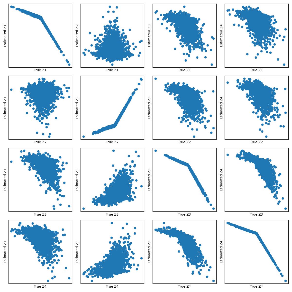
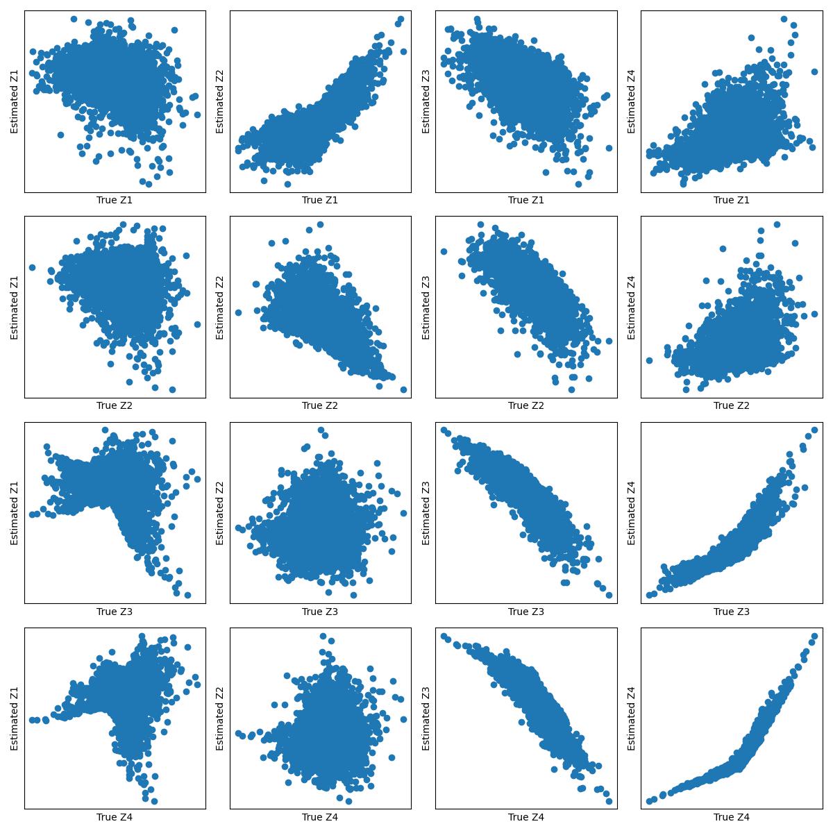
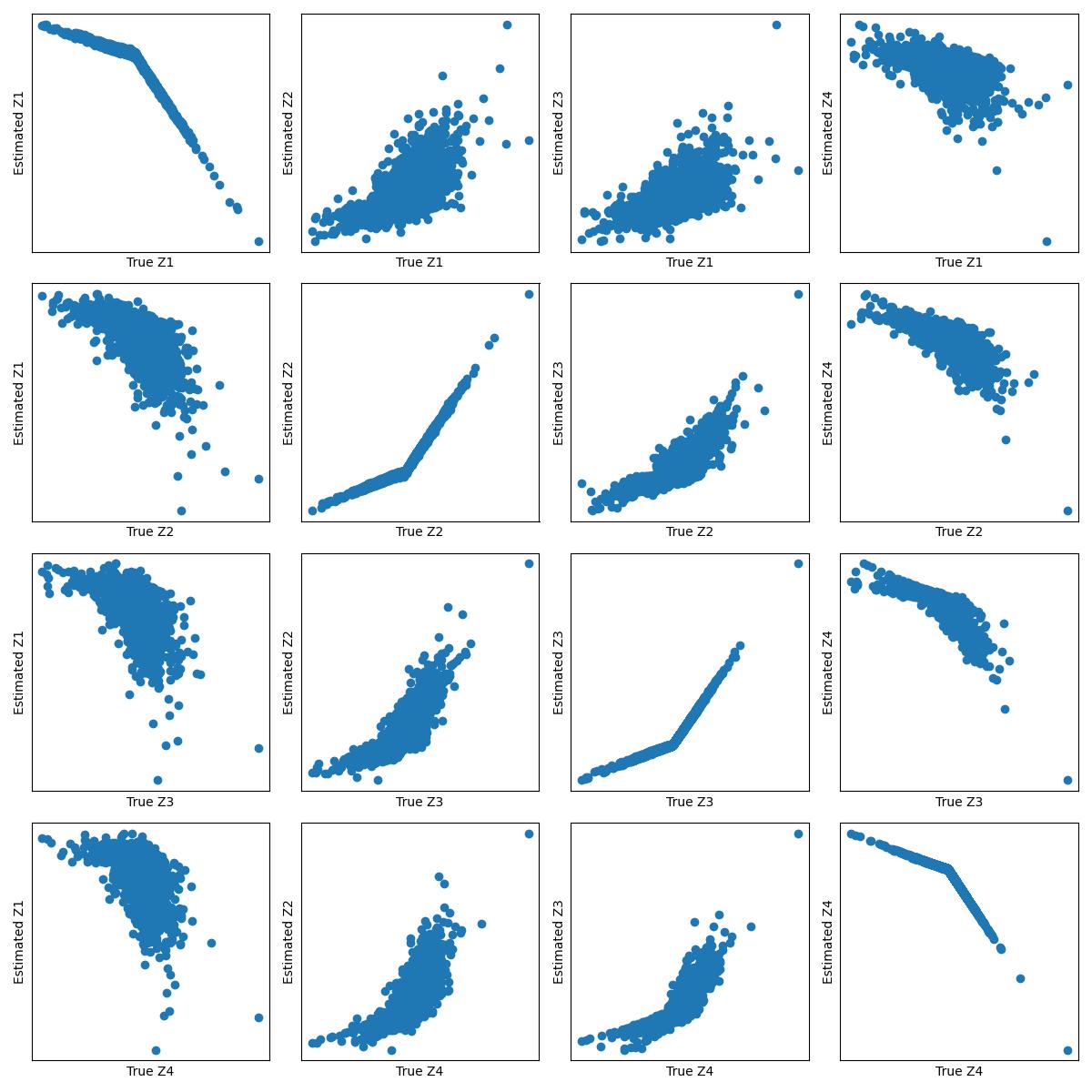
Figure 3: Recovered latent variables v.s. the true latent variables with Non-Parametric Approach. (a) Y-structure with Laplace noise. (b) Y-structure with Gaussian noise. (c) Chain structure with Laplace noise. (d) Chain structure with Gaussian noise. In each sub-figure, $i$-th row and $j$-th column depcits the relationship between the estimated $\hat{Z}_{i}$ and the true components $Z_{j}$.

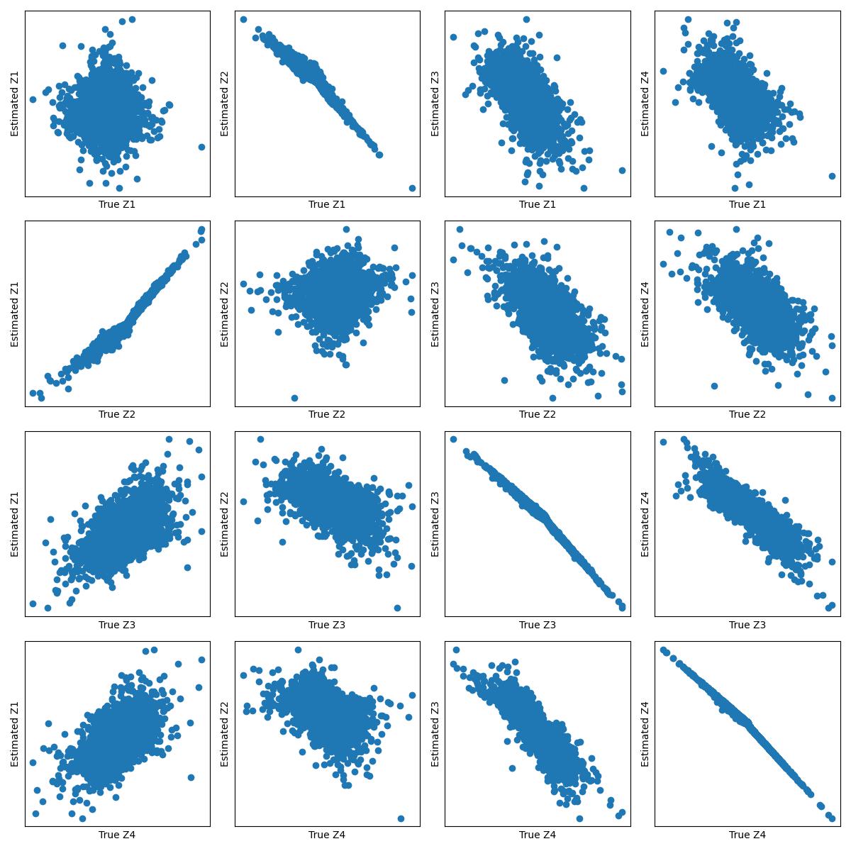
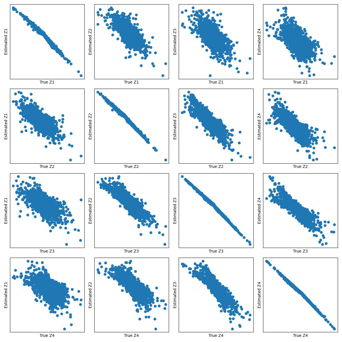
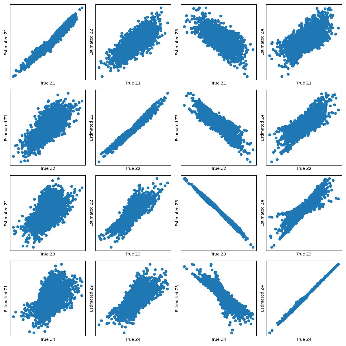
Figure 4: Recovered latent variables v.s. the true latent variables with Linear Parameterization Approach. The $X$-axis denotes the components of true latent variables $Z$ and the $Y$-axis represent the components of estimated latent variables $\hat{Z}$. (a) Y-structure with Laplace noise. (b) Y-structure with Gaussian noise. (c) Chain structure with Laplace noise. (d) Chain structure with Gaussian noise.

4.4 Simulations

To verify our theory and the proposed implementations, we run experiments on the simulated data because the ground truth causal adjacency matrix and the latent variables across domains are available for simulated data. Consequently, we consider following common causal structures (i) Y-structure with 4 variables, $Z_{1}\rightarrow Z_{3}\leftarrow Z_{2},Z_{3}\rightarrow Z_{4}$ and (ii) chain structure $Z_{1}\rightarrow Z_{2}\rightarrow Z_{3}\rightarrow Z_{4}$. The noises are modulated with scaling random sampled from $\operatorname{Unif}[0.5,2]$ and shifts are sampled from $\operatorname{Unif}[-2,2]$. The scaling on the $Z$ are also randomly sampled from $\operatorname{Unif}[0.5,2]$. In other words, the changes are modular. After generating $Z$, we feed the latent variables into MLP with orthogonal weights and LeakyReLU activations for invertibility. Specifically, we sample orthogonal matrix as the weights of the MLP layers. Since orthogonal matrix and LeakyReLU are invertible, the MLP function is also invertible.

We present the results in Fig. 3 and 4. Each sub-figure consist of $4\times 4$ panels and penal on $i$-th row and $j-th$column denotes the relationship between the estimated component $\hat{Z}_{i}$ with the true latent $Z_{j}$. We can see that under most cases, our model learns a strong one-to-one correspondence from the estimated components and the true components. For instance, the first column in Fig. 3 show that $\hat{Z}_{1}$ is strongly correlated with the true components $Z_{1}$ while it is nearly independent from the true $Z_{2}$.

From the estimated $\hat{A}$, we find that our method is able to recover the true causal struccture. For instance, on the $Y$ structure with $Z_{1}\rightarrow Z_{3}\leftarrow Z_{2}$ and $Z_{3}\rightarrow Z_{4}$, our estimated model only keep the components $\hat{A}_{1,3},\hat{A}_{2,3},\hat{A}_{3,4}$ nonzero with the proposed sparsity regularization. The estimated causal graph is consistent with the true $Y$-structure causal graph. We can also see that the latent causal structure is also recovered from Fig. 4 and 3. We observe that the learned $\hat{Z}_{1}$ is strongly correlated with the true $Z_{2}$ and is independent from the true $Z_{1}$, but correlated with the $\hat{Z}_{3}$ and $\hat{Z}_{4}$. These results aligns well with the true causal graph since $Z_{2}$ is independent from $Z_{1}$ while is the cause of $Z_{3}$ and $Z_{4}$.

The experiments support our theoretical result that the components and structure are identifiable up to certain indeterminacies. As for the results in Fig. 3, we observe that our non-parametric method is still able to recover the true latent variables with Laplace noise.

5 Related Work

Causal representation learning aims to unearth causal latent variables and their relations from observed data. Despite its significance, the identifiability of the hidden generating process is known to be impossible without additional constraints, especially with only observational data. In the linear, non-Gaussian case, Silva et al. (2006) recover the Markov equivalence class, provided that each observed variable has a unique latent causal parent; Xie et al. (2020); Cai et al. (2019) estimate the latent variables and their relations assuming at least twice measured variables as latent ones, which has been further extended to learn the latent hierarchical structure (Xie et al., 2022). Moreover, Adams et al. (2021) provide theoretical results on the graphical conditions for identification. In the linear, Gaussian case, Huang et al. (2022) leverage rank deficiency of the observed sub-covariance matrix to estimate the latent hierarchical structure. In the discrete case, Kivva et al. (2021) identify the hidden causal graph up to Markov equivalence by assuming a mixture model where the observed children sets of any pair of latent variables are different.

Given the challenge of identifiability on purely observational data, a different line of research leverage experiments by assuming the accessibility of various types of interventional data. Based on the single-node perfect intervention, Squires et al. (2023) leverage single-node interventions for the identifiability of linear causal model and linear mixing function; (Varici et al., 2023) incorporate for nonlinear causal model and linear mixing function; (Varici et al., 2023; Buchholz et al., 2023; Jiang & Aragam, 2023) provide the identifiability of the nonparametric causal model and linear mixing function; (Ahuja et al., 2023) further generalize the result to nonparametric causal model and polynomial mixing functions with additional constraints on the latent support; and (Brehmer et al., 2022; von Kügelgen et al., 2023; Jiang & Aragam, 2023) explore the nonparametric settings for both the causal model and mixing function. In addition to the single-node perfect interventions, Brehmer et al. (2022) introduced counterfactual pre- and post-intervention views; von Kügelgen et al. (2023) assume two distinct, paired interventions per node for multivariate causal models; and Jiang & Aragam (2023) places specific structural restrictions on the latent causal graph.

Our study lies in the line of leveraging only observational data, and provides identifiability results in the general nonparametric settings on both the latent causal model and mixing function. Unlike prior works with observational data, we do not have any parametric assumptions or graphical restrictions; Compared to those relying on interventional data, our results naturally benefit from the heterogeneity of observational data (e.g., multi-domain data, nonstationary time series) and avoid additional experiments for interventions.

6 Conclusion and Discussions

We establish a set of new identifiability results to reveal hidden causal variables and latent structures in the general nonparametric settings. Specifically, with sparsity regularization during estimation and sufficient changes in the causal influences, we demonstrate that the revealed hidden variables and structures are related to the underlying causal model in a specific, nontrivial way. In contrast to recent works on the recovery of hidden causal variables and structures, our results rely on purely observational data without graphical or parametric constraints. Our results offer insight into unveiling the latent causal process in one of the most universal settings. Experiments in various settings have been conducted to validate the theory. As future work, we will explore the scenario where only a subset of the causal relations change, which could be a challenge as well as a chance, and show up to what extent the underlying causal variables can be recovered with potentially weaker assumptions.

Appendix A Proof of Theorem 3.1

See 3.1

Proof.

Since $h$ in $\hat{Z}=h(Z)$ is invertible, we have

$$p(\hat{Z};\hat{\theta}) =p(Z;\theta)/|J_{h}|,$$

$$\log p(\hat{Z};\hat{\theta}) =\log p(Z;\theta)-\log|J_{h}|.$$ (15)

Suppose $\hat{Z}_{k}$ and $\hat{Z}_{l}$ are conditionally independent given $\hat{Z}_{[n]\setminus\{k,l\}}$ i.e., they are not adjacent in the Markov network over $\hat{Z}$. For each $\theta$, by Lin (1997), we have

$$\frac{\partial^{2}\log p(\hat{Z};\hat{\theta})}{\partial\hat{Z}_{k}\partial\hat{Z}_{l}}=0.$$

To see what it implies, we find the first-order derivative:

$$\frac{\partial\log p(\hat{Z};\theta)}{\partial\hat{Z}_{k}}=\sum_{i}\frac{\partial\log p({Z};\theta)}{\partial Z_{i}}\frac{\partial Z_{i}}{\partial\hat{Z}_{k}}-\frac{\partial\log|J_{q}|}{\partial\hat{Z}_{k}}.$$

Let $\eta(\theta)=\log p(Z;\theta)$, $\eta^{\prime}_{i}(\theta)=\frac{\partial\log p(Z;\theta)}{\partial Z_{i}}$, $\eta^{\prime\prime}_{ij}(\theta)=\frac{\partial^{2}\log p({Z};\theta)}{\partial Z_{i}\partial Z_{j}}$, $h^{\prime}_{i,l}=\frac{\partial Z_{i}}{\partial\hat{Z}_{l}}$, and $h^{\prime\prime}_{i,kl}=\frac{\partial^{2}Z_{i}}{\partial\hat{Z}_{k}\partial\hat{Z}_{l}}$. We then derive the second-order derivative:

$$0= \sum_{j}\sum_{i}\frac{\partial^{2}\log p({Z};\theta)}{\partial Z_{i}\partial Z_{j}}\frac{\partial Z_{j}}{\partial\hat{Z}_{l}}\frac{\partial Z_{i}}{\partial\hat{Z}_{k}}+\sum_{i}\frac{\partial\log p({Z};\theta)}{\partial Z_{i}}\frac{\partial^{2}Z_{i}}{\partial\hat{Z}_{k}\partial\hat{Z}_{l}}-\frac{\partial^{2}\log|J_{q}|}{\partial\hat{Z}_{k}\partial\hat{Z}_{l}}.$$

$$= \sum_{i}\frac{\partial^{2}\log p({Z};\theta)}{\partial Z_{i}^{2}}\frac{\partial Z_{i}}{\partial\hat{Z}_{l}}\frac{\partial Z_{i}}{\partial\hat{Z}_{k}}+\sum_{j}\sum_{(j,i)\in\mathcal{E}(\mathcal{M}_{Z})}\frac{\partial^{2}\log p({Z};\theta)}{\partial Z_{i}\partial Z_{j}}\frac{\partial Z_{j}}{\partial\hat{Z}_{l}}\frac{\partial Z_{i}}{\partial\hat{Z}_{k}}$$

$$\qquad+\sum_{i}\frac{\partial\log p({Z};\theta)}{\partial Z_{i}}\frac{\partial^{2}Z_{i}}{\partial\hat{Z}_{k}\partial\hat{Z}_{l}}-\frac{\partial^{2}\log|J_{q}|}{\partial\hat{Z}_{k}\partial\hat{Z}_{l}}$$

$$= \sum_{i}\eta^{\prime\prime}_{ii}(\theta)h^{\prime}_{i,l}h^{\prime}_{i,k}+\sum_{j}\sum_{(j,i)\in\mathcal{E}(\mathcal{M}_{Z})}\eta^{\prime\prime}_{ij}(\theta)h^{\prime}_{j,l}h^{\prime}_{i,k}+\sum_{i}\eta^{\prime}_{i}(\theta)h^{\prime\prime}_{i,kl}-\frac{\partial^{2}\log|J_{q}|}{\partial\hat{Z}_{k}\partial\hat{Z}_{l}}.$$ (16)

Here we denote by $\mathcal{E}(\mathcal{M}_{Z})$ the set of edges in the Markov network over $Z$ and we already make use of the fact that if $Z_{i}$ and $Z_{j}$ are not adjacent in the Markov network, then $\frac{\partial^{2}\log p(Z;\theta)}{\partial Z_{i}\partial Z_{j}}=0$.

By Assumption A2, consider the $2n+|\mathcal{M}_{Z}|+1$ values of $\theta$, i.e., $\theta^{(u)}$ with $u=0,\dots,2n+|\mathcal{M}_{Z}|$, such that Eq. (16) hold. Then, we have $2n+|\mathcal{M}_{Z}|+1$ such equations. Subtracting each equation corresponding to $\theta^{(u)},u=1,\dots,2n+|\mathcal{M}_{Z}|$ with the equation corresponding to $\theta^{(0)}$ resuls in $2n+|\mathcal{M}_{Z}|$ equations:

$$0 =\sum_{i}(\eta^{\prime\prime}_{ii}(\theta^{(u)})-\eta^{\prime\prime}_{ii}(\theta^{(0)}))h^{\prime}_{i,l}h^{\prime}_{i,k}+\sum_{j}\sum_{(j,i)\in\mathcal{E}(\mathcal{M}_{Z})}(\eta^{\prime\prime}_{ij}(\theta^{(u)})-\eta^{\prime\prime}_{ij}(\theta^{(0)}))h^{\prime}_{j,l}h^{\prime}_{i,k}$$

$$\qquad+\sum_{i}(\eta^{\prime}_{i}(\theta^{(u)})-\eta^{\prime}_{i}(\theta^{(0)}))h^{\prime\prime}_{i,kl},$$

where $u=1,\dots,2n+|\mathcal{M}_{Z}|$. By Assumption A2, the vectors formed by collecting the corresponding coefficients are linearly independent. Therefore, for any $i$ and any $j$ such that $(j,i)\in\mathcal{E}(\mathcal{M}_{Z})$, we have

$$h^{\prime}_{i,l}h^{\prime}_{i,k} =0,$$ (17)

$$h^{\prime}_{j,l}h^{\prime}_{i,k} =0,$$ (18)

$$h^{\prime\prime}_{i,kl} =0.$$ (19)

Eq. (17) indicates that $Z_{i}$ is a function of at most one of $\hat{Z}_{k}$ and $\hat{Z}_{l}$, while Eq. (18) implies that given that $Z_{i}$ and $Z_{j}$ are adjacent in Markov network $\mathcal{M}_{Z}$, at most one of them is a function of $\hat{Z}_{k}$ or $\hat{Z}_{l}$. ∎

Appendix B Proof of Theorem 3.2

First, we introduce the following lemma, which will be used in the proof.

Lemma 2.

For any invertible matrix $A$, there exists a permutation of its row such that the diagonal entries of the resulting matrix are nonzero.

Proof.

Suppose by contradiction that there exists at least a zero diagonal entry for every row permutation. By Leibniz formula, we have

$$\det(A)=\sum_{\sigma\in\mathcal{S}_{n}}\left(\operatorname{sgn}(\sigma)\prod_{i=1}^{n}a_{\sigma(i),i}\right),$$

where $\mathcal{S}_{n}$ denotes the set of $n$-permutations. Since there exists a zero diagonal entry for every permutation, we have

$$\prod_{i=1}^{n}a_{\sigma(i),i}=0,\quad\forall\sigma\in\mathcal{S}_{n},$$

which implies $\det(A)=0$ and that matrix $A$ is not invertible. This is a contradiciton with the assumption that $A$ is invertible. ∎

See 3.2

Proof.

Based on Lemma 2, there exists a permutation $\pi$ of the estimated hidden variables, denoted as $\hat{Z}_{\pi}$, such that

$$\frac{\partial Z_{i}}{\partial\hat{Z}_{\pi(i)}}\neq 0,\quad i=1,\dots,n.$$ (20)

Suppose that $Z_{i}$ and $Z_{j}$ are adjacent in the Markov network $\mathcal{M}_{Z}$ over $Z$, but $\tilde{Z}_{\pi(i)}$ and $\tilde{Z}_{\pi(i)}$ are not adjacent in the Markov network $\mathcal{M}_{\hat{Z}}$ over $\hat{Z}$. By Theorem 3.1, at most one of $Z_{i}$ and $Z_{j}$ is a function of $\tilde{Z}_{\pi(i)}$ and $\tilde{Z}_{\pi(i)}$. This is clearly a contradiction with Eq. (20).

Therefore, we have shown by contradiction that, if $Z_{i}$ and $Z_{j}$ are adjacent in the Markov network $\mathcal{M}_{Z}$ over $Z$, then $\tilde{Z}_{\pi(i)}$ and $\tilde{Z}_{\pi(i)}$ are adjacent in the Markov network $\mathcal{M}_{\hat{Z}_{\pi}}$ over variables $\hat{Z}_{\pi}$. That is, all edges in $\mathcal{M}_{Z}$ must be present in Markov network $\mathcal{M}_{\hat{Z}_{\pi}}$ over variables $\hat{Z}_{\pi}$. Also, note that the true model $(g,f,p_{Z})$ is clearly one of the solutions that achieves Eq. (2). Thus, under sparsity constraint on the edges of $\mathcal{M}_{\hat{Z}}$, we conclude that the Markov network $\mathcal{M}_{\hat{Z}_{\pi}}$ over $\hat{Z}_{\pi}$ must be identical to the Markov network $\mathcal{M}_{Z}$ over $Z$, ∎

Appendix C Proof of Corollary 3.3

Suppose by contradiction that $(\hat{g},\hat{f},p_{\hat{Z}})$ achieves Eq. (2). By assumption, the components of $\hat{Z}$ are independent in each domain, indicating that the Markov network $\mathcal{M}_{\hat{Z}}$ is an empty graph. By similar reasoning in the proof of Theorem 3.2, all edges in the true Markov network $\mathcal{M}_{Z}$ must be present in $\mathcal{M}_{\hat{Z}}$ (up to isomorphism). Since $\mathcal{M}_{\hat{Z}}$ is an empty graph, this implies that $\mathcal{M}_{Z}$ is also an empty graph, which is contradictory with the assumption that $\mathcal{M}_{Z}$ is not an empty graph.

Appendix D Proof of Theorem 3.4

We first state the following lemma that is used to prove Statement (b) of Theorem 3.4. The proof is a straightforward consequence of Cayley–Hamilton theorem and is omitted here.

Lemma 3.

Let $A$ be an $n\times n$ invertible matrix. Then, it can be expressed as a linear combination of the powers of $A$, i.e.,

$$A^{-1}=\sum_{k=0}^{n-1}c_{k}A^{k}$$

for some appropriate choice of coefficients $c_{0},c_{1},\dots,c_{n-1}$.

Now consider the Markov network $\mathcal{M}_{Z}$ over hidden causal variables $Z$. Let $N_{Z_{i}}$ be the set of neighbors of $Z_{i}$ in $\mathcal{M}_{Z}$. We provide the following result that relates a matrix to its inverse, given that such matrix satisfies certain property defined by $\mathcal{M}_{Z}$.

Proposition 1.

Consider a Markov network $\mathcal{M}_{Z}$ over $Z$. Let $N_{Z_{i}}$ be the set of neighbors of $Z_{i}$ in $\mathcal{M}_{Z}$, and $A$ be an $n\times n$ invertible matrix. For each $i\neq j$ where $Z_{j}$ is not adjacent to some nodes in $\{Z_{i}\}\cup N_{Z_{i}}$, suppose $A_{ij}=0$. Then, we have $A^{-1}_{ij}=0$.

Proof.

By Lemma 3, $A^{-1}$ can be expressed as linear combination of the powers of $A$. Therefore, it suffices to prove that, each matrix power $A^{k}$ satisfies the following property: $A^{k}_{ij}=0$ for each $i\neq j$ where $Z_{j}$ is not adjacent to some nodes in $\{Z_{i}\}\cup N_{Z_{i}}$. We proceed with mathematical induction on $k$. By definition, the property holds in the base case where $k=1$.

Now suppose that the property holds for $A^{k}$. We prove by contradiction that the property holds for $A^{k+1}$. Suppose by contradiction that $A^{k+1}_{ij}\neq 0$ for some $i\neq j$ where $Z_{j}$ is not adjacent to some nodes in $\{Z_{i}\}\cup N_{Z_{i}}$. This implies that one of the following cases holds:

• Case (a): $Z_{j}$ is not adjacent to $Z_{i}$ in $\mathcal{M}_{G_{Z}}$.

• Case (b): There exists $Z_{l}\in N_{Z_{i}}\setminus\{Z_{j}\}$ such that $Z_{j}$ and $Z_{l}$ are not adjacent in $\mathcal{M}_{G_{Z}}$.

Since $A^{k+1}_{ij}=\sum_{r=0}^{n}A^{k}_{ir}A_{rj}$, the assumption $A^{k+1}_{ij}\neq 0$ implies that there must exist $m$ such that $A^{k}_{im}A_{mj}\neq 0$, i.e., $A^{k}_{im}\neq 0$ and $A_{mj}\neq 0$. Since both $A^{k}$ and $A$ satisfy the property, this indicates (i) $Z_{m}$ is adjacent to $Z_{i}$ and all nodes in $N_{Z_{i}}\setminus\{Z_{m}\}$, and (ii) $Z_{j}$ is adjacent to $Z_{m}$ and all nodes in $N_{Z_{m}}\setminus\{Z_{j}\}$. We consider the following cases:

• Case of $m=l$: By (ii), $Z_{j}$ is adjacent to $Z_{l}$, which contradicts Case (b) above. Also, we know that $Z_{l}$ is adjacent to $Z_{i}$ by (i), which indicates that $Z_{i}$ is adjacent to $Z_{j}$, contradicting Case (a) above.

• Case of $m\neq l$: By (i) and (ii), $Z_{m}$ is adjacent to $Z_{i}$ and $Z_{j}$ is adjacent to $Z_{m}$, implying that $Z_{i}$ and $Z_{j}$ are adjacent, which is contradictory with Case (a) above. Furthermore, since $Z_{l}$ is a neighbor of $Z_{i}$, we know that $Z_{m}$ and $Z_{l}$ are adjacent by (i). Also, by (ii), $Z_{j}$ is adjacent to $Z_{l}$, which contradicts Case (b) above.

In either of the cases above, there is a contradiction. ∎

We are now ready to give the following result. See 3.4

Proof.

We first prove a simpler case: there exists a permutation $\pi$ of the estimated hidden variables, denoted as $\hat{Z}_{\pi}$, such that $Z_{i}$ is a function of $\hat{Z}_{\pi(i)}$ and a subset of the variables in $\{\hat{Z}_{\pi(j)}\,|\,Z_{j}\textrm{ is adjacent to }Z_{i}\textrm{ and all other neighbors of }Z_{i}\textrm{ in }\mathcal{M}_{Z}\}$.

By Theorem 3.2 and its proof, there exists a permutation $\pi$ of the estimated variables, denoted as $\hat{Z}_{\pi}$, such that the Markov network $\mathcal{M}_{\hat{Z}_{\pi}}$ over $\hat{Z}_{\pi}$ is identical to $\mathcal{M}_{Z}$, and that

$$\frac{\partial Z_{i}}{\partial\hat{Z}_{\pi(i)}}\neq 0,\quad i=1,\dots,n.$$

Clearly, each variable $Z_{i}$ is a function of $\hat{Z}_{\pi(i)}$.

We first show that if $Z_{j}$ is not adjacent to $Z_{i}$ in $\mathcal{M}_{Z}$, then $Z_{i}$ cannot be a function of $\hat{Z}_{\pi(j)}$. Since $Z_{i}$ and $Z_{j}$ are not adjacent in $\mathcal{M}_{Z}$, we know that $\hat{Z}_{\pi(i)}$ and $\hat{Z}_{\pi(j)}$ are not adjacent in $\mathcal{M}_{{\hat{Z}_{\pi}}}$. By Theorem 3.1, $Z_{i}$ is a function of at most one of $\hat{Z}_{\pi(i)}$ and $\hat{Z}_{\pi(j)}$, which implies that $Z_{i}$ cannot be a function of $\hat{Z}_{\pi(j)}$, because we have shown that $Z_{i}$ is a function of $\hat{Z}_{\pi(i)}$.

To refine further, now suppose that $Z_{j}$ is adjacent to $Z_{i}$, but not adjacent to some $Z_{k}\in N_{Z_{i}}\setminus\{Z_{j}\}$. Since $\mathcal{M}_{Z}$ and $\mathcal{M}_{{\hat{Z}_{\pi}}}$ are identical, $\hat{Z}_{\pi(j)}$ is also not adjacent to $\hat{Z}_{\pi(k)}$ in $\mathcal{M}_{\hat{Z}_{\pi}}$. Since $Z_{i}$ and $Z_{k}$ are adjacent in $\mathcal{M}_{Z}$, by Theorem 3.1, at most one of them is a function of $\hat{Z}_{{\pi(j)}}$ or $\hat{Z}_{\pi(k)}$. This implies that $Z_{i}$ cannot be a function of $\hat{Z}_{\pi(j)}$, because we have shown that $Z_{k}$ is a function of $\hat{Z}_{\pi(k)}$.

Therefore, we have just shown that $Z_{i}$ is a function of at most the variables in

$$\hat{Z}_{\pi(i)}\cup\{\hat{Z}_{\pi(j)}\,|\,Z_{j}\textrm{ is adjacent to }Z_{i}\textrm{ and all other neighbors of }Z_{i}\textrm{ in }\mathcal{M}_{Z}\}.$$

Now for each $k\neq i$ where $Z_{i}$ is not adjacent to some nodes in $\{Z_{k}\}\cup N_{Z_{k}}$, we have

$$\frac{\partial Z_{k}}{\partial\hat{Z}_{\pi(i)}}=0.$$

By Proposition 1, we have

$$\left(\frac{\partial Z}{\partial\hat{Z}_{\pi}}\right)^{-1}_{ki}=0,$$

which, by inverse function theorem, implies

$$\frac{\partial\hat{Z}_{\pi(i)}}{\partial Z_{k}}=\left(\frac{\partial Z}{\partial\hat{Z}_{\pi}}\right)^{-1}_{ki}=0.$$

This implies that $\hat{Z}_{\pi(i)}$ cannot be a function of $Z_{k}$. ∎

Appendix E Proof of Lemma 1 and Theorem 3.5

See 1

Proof.

Let $Z_{j}$ and $Z_{k}$, $j\neq k$ be two variables that $i$ and $j$ are not adjacent in the moralized graph of $\mathcal{G}_{Z}$. Then it suffices to show that $(j,k)\notin\mathcal{E}(\mathcal{M}_{Z})$ and $(k,j)\notin\mathcal{E}(\mathcal{M}_{Z})$. Because they are not adjacent in the moralized graph of $\mathcal{G}_{Z}$, they must not be adjacent in $\mathcal{G}_{Z}$ and must not share a common child in $\mathcal{G}_{Z}$. Thus, $j$ and $k$ are d-separated conditioning on $V\setminus\{j,k\}$, which implies the conditional independence $Z_{j}\mathchoice{\mathrel{\hbox to0.0pt{$\displaystyle\perp$\hss}\mkern 2.0mu{\displaystyle\perp}}}{\mathrel{\hbox to0.0pt{$\textstyle\perp$\hss}\mkern 2.0mu{\textstyle\perp}}}{\mathrel{\hbox to0.0pt{$\scriptstyle\perp$\hss}\mkern 2.0mu{\scriptstyle\perp}}}{\mathrel{\hbox to0.0pt{$\scriptscriptstyle\perp$\hss}\mkern 2.0mu{\scriptscriptstyle\perp}}}Z_{k}|Z\setminus\{Z_{j},Z_{k}\}$ based on the Markov assumption on $\{\mathcal{G}_{Z},P_{Z}\}$. Then we have $(j,k)\notin\mathcal{E}(\mathcal{M}_{Z})$ and $(k,j)\notin\mathcal{E}(\mathcal{M}_{Z})$. ∎

See 3.5

Proof.

We prove both directions as follows.

Sufficient condition.   We prove it by contradiction. Suppose that the structure defined by $\operatorname{supp}(\mathcal{M}_{Z})$ is not equivalent to the moralized graph of $\mathcal{G}_{Z}$. Then, according to Lem. 1, there exists a pair of variables $Z_{j}$ and $Z_{k}$, $j\neq k$ that $i$ and $j$ are adjacent in the moralized graph but $(j,k)\notin\mathcal{E}(\mathcal{M}_{Z})$ and $(k,j)\notin\mathcal{E}(\mathcal{M}_{Z})$. Thus, we have $Z_{j}\mathchoice{\mathrel{\hbox to0.0pt{$\displaystyle\perp$\hss}\mkern 2.0mu{\displaystyle\perp}}}{\mathrel{\hbox to0.0pt{$\textstyle\perp$\hss}\mkern 2.0mu{\textstyle\perp}}}{\mathrel{\hbox to0.0pt{$\scriptstyle\perp$\hss}\mkern 2.0mu{\scriptstyle\perp}}}{\mathrel{\hbox to0.0pt{$\scriptscriptstyle\perp$\hss}\mkern 2.0mu{\scriptscriptstyle\perp}}}Z_{k}|Z\setminus\{Z_{j},Z_{k}\}$. Then we consider the following two cases:

• If variables $Z_{j}$ and $Z_{k}$ correspond to a pair of neighbors in $\mathcal{G}_{Z}$, then they are adjacent. Together with the conditional independence relation $Z_{j}\mathchoice{\mathrel{\hbox to0.0pt{$\displaystyle\perp$\hss}\mkern 2.0mu{\displaystyle\perp}}}{\mathrel{\hbox to0.0pt{$\textstyle\perp$\hss}\mkern 2.0mu{\textstyle\perp}}}{\mathrel{\hbox to0.0pt{$\scriptstyle\perp$\hss}\mkern 2.0mu{\scriptstyle\perp}}}{\mathrel{\hbox to0.0pt{$\scriptscriptstyle\perp$\hss}\mkern 2.0mu{\scriptscriptstyle\perp}}}Z_{k}|Z\setminus\{Z_{j},Z_{k}\}$, this implies that the SAF assumption is violated.

• If variables $Z_{j}$ and $Z_{k}$ correspond to a pair of non-adjacent spouses in $\mathcal{G}_{Z}$. Then they have an unshielded collider, indicating that the SUCF assumption is violated.

Necessary condition.   We prove it by contradiction. Suppose SUCF or SAF is violated, we have the following two cases:

• Suppose SUCF is violated, i.e., there exists an unshielded collider $j\rightarrow i\leftarrow k$ in the DAG $\mathcal{G}_{Z}$ such that $Z_{j}\mathchoice{\mathrel{\hbox to0.0pt{$\displaystyle\perp$\hss}\mkern 2.0mu{\displaystyle\perp}}}{\mathrel{\hbox to0.0pt{$\textstyle\perp$\hss}\mkern 2.0mu{\textstyle\perp}}}{\mathrel{\hbox to0.0pt{$\scriptstyle\perp$\hss}\mkern 2.0mu{\scriptstyle\perp}}}{\mathrel{\hbox to0.0pt{$\scriptscriptstyle\perp$\hss}\mkern 2.0mu{\scriptscriptstyle\perp}}}Z_{k}|Z\setminus\{Z_{j},Z_{k}\}$. This conditional independence relation indicates that $(j,k)\notin\mathcal{E}(\mathcal{M}_{Z})$ and $(k,j)\notin\mathcal{E}(\mathcal{M}_{Z})$. Since $j$ and $k$ are spouses, there exists an edge between them in the moralized graph of $\mathcal{G}_{Z}$, but is not contained in the structure defined by $\mathcal{M}_{Z}$, showing that they are not the same.

• Or, suppose SAF is violated, i.e., there exists a pair of neighbors $j$ and $k$ in the DAG $\mathcal{G}_{Z}$ such that $Z_{j}\mathchoice{\mathrel{\hbox to0.0pt{$\displaystyle\perp$\hss}\mkern 2.0mu{\displaystyle\perp}}}{\mathrel{\hbox to0.0pt{$\textstyle\perp$\hss}\mkern 2.0mu{\textstyle\perp}}}{\mathrel{\hbox to0.0pt{$\scriptstyle\perp$\hss}\mkern 2.0mu{\scriptstyle\perp}}}{\mathrel{\hbox to0.0pt{$\scriptscriptstyle\perp$\hss}\mkern 2.0mu{\scriptscriptstyle\perp}}}Z_{k}|Z\setminus\{Z_{j},Z_{k}\}$. This conditional independence relation indicates that $(j,k)\notin\mathcal{E}(\mathcal{M}_{Z})$ and $(k,j)\notin\mathcal{E}(\mathcal{M}_{Z})$. Because $j$ and $k$ are adjacent in $\mathcal{G}_{Z}$, clearly they are also adjacent in the moralized graph of $\mathcal{G}_{Z}$. However, the edge between them is not contained in the structure defined by $\mathcal{M}_{Z}$, showing that they are not the same.

Thus, when SUCF or SAF is violated, the structure defined by $\mathcal{M}_{Z}$ is the moralized graph of the true DAG $\mathcal{G}_{Z}$. ∎

References

- Adams et al. (2021) Adams, J., Hansen, N., and Zhang, K. Identification of partially observed linear causal models: Graphical conditions for the non-gaussian and heterogeneous cases. Advances in Neural Information Processing Systems, 34:22822–22833, 2021.
- Ahuja et al. (2023) Ahuja, K., Mahajan, D., Wang, Y., and Bengio, Y. Interventional causal representation learning. In International Conference on Machine Learning, pp. 372–407. PMLR, 2023.
- Brehmer et al. (2022) Brehmer, J., De Haan, P., Lippe, P., and Cohen, T. S. Weakly supervised causal representation learning. Advances in Neural Information Processing Systems, 35:38319–38331, 2022.
- Buchholz et al. (2022) Buchholz, S., Besserve, M., and Schölkopf, B. Function classes for identifiable nonlinear independent component analysis. arXiv preprint arXiv:2208.06406, 2022.
- Buchholz et al. (2023) Buchholz, S., Rajendran, G., Rosenfeld, E., Aragam, B., Schölkopf, B., and Ravikumar, P. Learning linear causal representations from interventions under general nonlinear mixing. arXiv preprint arXiv:2306.02235, 2023.
- Cai et al. (2019) Cai, R., Xie, F., Glymour, C., Hao, Z., and Zhang, K. Triad constraints for learning causal structure of latent variables. Advances in neural information processing systems, 32, 2019.
- Comon (1994) Comon, P. Independent component analysis – a new concept? Signal Processing, 36:287–314, 1994.
- Hälvä & Hyvärinen (2020) Hälvä, H. and Hyvärinen, A. Hidden markov nonlinear ICA: Unsupervised learning from nonstationary time series. In Conference on Uncertainty in Artificial Intelligence, pp. 939–948. PMLR, 2020.
- Hälvä et al. (2021) Hälvä, H., Le Corff, S., Lehéricy, L., So, J., Zhu, Y., Gassiat, E., and Hyvärinen, A. Disentangling identifiable features from noisy data with structured nonlinear ICA. Advances in Neural Information Processing Systems, 34, 2021.
- Huang et al. (2022) Huang, B., Low, C. J. H., Xie, F., Glymour, C., and Zhang, K. Latent hierarchical causal structure discovery with rank constraints. Advances in Neural Information Processing Systems, 35:5549–5561, 2022.
- Hyvärinen & Morioka (2016) Hyvärinen, A. and Morioka, H. Unsupervised feature extraction by time-contrastive learning and nonlinear ICA. Advances in Neural Information Processing Systems, 29:3765–3773, 2016.
- Hyvärinen & Morioka (2017) Hyvärinen, A. and Morioka, H. Nonlinear ICA of temporally dependent stationary sources. In International Conference on Artificial Intelligence and Statistics, pp. 460–469. PMLR, 2017.
- Hyvärinen & Pajunen (1999) Hyvärinen, A. and Pajunen, P. Nonlinear independent component analysis: Existence and uniqueness results. Neural networks, 12(3):429–439, 1999.
- Hyvärinen et al. (1999) Hyvärinen, A., Cristescu, R., and Oja, E. A fast algorithm for estimating overcomplete ICA bases for image windows. In Proc. Int. Joint Conf. on Neural Networks, pp. 894–899, Washington, D.C., 1999.
- Hyvärinen et al. (2019) Hyvärinen, A., Sasaki, H., and Turner, R. Nonlinear ICA using auxiliary variables and generalized contrastive learning. In International Conference on Artificial Intelligence and Statistics, pp. 859–868. PMLR, 2019.
- Hyvärinen et al. (2023) Hyvärinen, A., Khemakhem, I., and Morioka, H. Nonlinear independent component analysis for principled disentanglement in unsupervised deep learning. Patterns, 4(10):100844, 2023. ISSN 2666-3899. doi: https://doi.org/10.1016/j.patter.2023.100844. URL https://www.sciencedirect.com/science/article/pii/S2666389923002234.
- Jiang & Aragam (2023) Jiang, Y. and Aragam, B. Learning nonparametric latent causal graphs with unknown interventions. arXiv preprint arXiv:2306.02899, 2023.
- Khemakhem et al. (2020a) Khemakhem, I., Kingma, D., Monti, R., and Hyvärinen, A. Variational autoencoders and nonlinear ICA: A unifying framework. In International Conference on Artificial Intelligence and Statistics, pp. 2207–2217. PMLR, 2020a.
- Khemakhem et al. (2020b) Khemakhem, I., Monti, R., Kingma, D., and Hyvarinen, A. Ice-beem: Identifiable conditional energy-based deep models based on nonlinear ica. Advances in Neural Information Processing Systems, 33:12768–12778, 2020b.
- Kingma & Welling (2013) Kingma, D. P. and Welling, M. Auto-encoding variational bayes. arXiv preprint arXiv:1312.6114, 2013.
- Kivva et al. (2021) Kivva, B., Rajendran, G., Ravikumar, P., and Aragam, B. Learning latent causal graphs via mixture oracles. Advances in Neural Information Processing Systems, 34:18087–18101, 2021.
- Kong et al. (2022) Kong, L., Xie, S., Yao, W., Zheng, Y., Chen, G., Stojanov, P., Akinwande, V., and Zhang, K. Partial disentanglement for domain adaptation. In International Conference on Machine Learning, pp. 11455–11472. PMLR, 2022.
- Lachapelle et al. (2022) Lachapelle, S., López, P. R., Sharma, Y., Everett, K., Priol, R. L., Lacoste, A., and Lacoste-Julien, S. Disentanglement via mechanism sparsity regularization: A new principle for nonlinear ICA. Conference on Causal Learning and Reasoning, 2022.
- Lin (1997) Lin, J. Factorizing multivariate function classes. Advances in neural information processing systems, 10, 1997.
- Loh & Bühlmann (2014) Loh, P.-L. and Bühlmann, P. High-dimensional learning of linear causal networks via inverse covariance estimation. The Journal of Machine Learning Research, 15(1):3065–3105, 2014.
- Ng et al. (2021) Ng, I., Zheng, Y., Zhang, J., and Zhang, K. Reliable causal discovery with improved exact search and weaker assumptions. In Advances in Neural Information Processing Systems, 2021.
- Pearl (2000) Pearl, J. Causality: Models, Reasoning, and Inference. Cambridge University Press, Cambridge, 2000.
- Ramsey et al. (2012) Ramsey, J., Zhang, J., and Spirtes, P. L. Adjacency-faithfulness and conservative causal inference. arXiv preprint arXiv:1206.6843, 2012.
- Schölkopf et al. (2021) Schölkopf, B., Locatello, F., Bauer, S., Ke, N. R., Kalchbrenner, N., Goyal, A., and Bengio, Y. Towards causal representation learning. Proceedings of the IEEE, 109(5):612–634, 2021.
- Silva et al. (2006) Silva, R., Scheines, R., Glymour, C., and Spirtes, P. Learning the structure of linear latent variable models. Journal of Machine Learning Research, 7:191–246, 2006.
- Sorrenson et al. (2020) Sorrenson, P., Rother, C., and Köthe, U. Disentanglement by nonlinear ICA with general incompressible-flow networks (GIN). arXiv preprint arXiv:2001.04872, 2020.
- Spirtes et al. (2001) Spirtes, P., Glymour, C., and Scheines, R. Causation, Prediction, and Search. MIT Press, Cambridge, MA, 2nd edition, 2001.
- Squires et al. (2023) Squires, C., Seigal, A., Bhate, S. S., and Uhler, C. Linear causal disentanglement via interventions. In International Conference on Machine Learning, 2023.
- Taleb & Jutten (1999) Taleb, A. and Jutten, C. Source separation in post-nonlinear mixtures. IEEE Transactions on signal Processing, 47(10):2807–2820, 1999.
- Uhler et al. (2013) Uhler, C., Raskutti, G., Bühlmann, P., and Yu, B. Geometry of the faithfulness assumption in causal inference. The Annals of Statistics, pp. 436–463, 2013.
- Varici et al. (2023) Varici, B., Acarturk, E., Shanmugam, K., Kumar, A., and Tajer, A. Score-based causal representation learning with interventions. arXiv preprint arXiv:2301.08230, 2023.
- von Kügelgen et al. (2023) von Kügelgen, J., Besserve, M., Liang, W., Gresele, L., Kekić, A., Bareinboim, E., Blei, D. M., and Schölkopf, B. Nonparametric identifiability of causal representations from unknown interventions. arXiv preprint arXiv:2306.00542, 2023.
- Xie et al. (2020) Xie, F., Cai, R., Huang, B., Glymour, C., Hao, Z., and Zhang, K. Generalized independent noise condition for estimating latent variable causal graphs. In Advances in Neural Information Processing Systems, 2020.
- Xie et al. (2022) Xie, F., Huang, B., Chen, Z., He, Y., Geng, Z., and Zhang, K. Identification of linear non-gaussian latent hierarchical structure. In International Conference on Machine Learning, pp. 24370–24387. PMLR, 2022.
- Xie et al. (2023) Xie, S., Zhang, Z., Lin, Z., Hinz, T., and Zhang, K. SmartBrush: Text and shape guided object inpainting with diffusion model. In Proceedings of the IEEE/CVF Conference on Computer Vision and Pattern Recognition, pp. 620–629, 2023.
- Yao et al. (2021) Yao, W., Sun, Y., Ho, A., Sun, C., and Zhang, K. Learning temporally causal latent processes from general temporal data. arXiv preprint arXiv:2110.05428, 2021.
- Yao et al. (2022) Yao, W., Chen, G., and Zhang, K. Temporally disentangled representation learning. In Advances in Neural Information Processing Systems, 2022.
- Zhang & Spirtes (2008) Zhang, J. and Spirtes, P. Detection of unfaithfulness and robust causal inference. Minds and Machines, 18:239–271, 2008.
- Zheng et al. (2022) Zheng, Y., Ng, I., and Zhang, K. On the identifiability of nonlinear ICA: Sparsity and beyond. In Advances in Neural Information Processing Systems, 2022.